chambers creek dye study: final model simulation report · chambers creek . dye study . final model...

Chambers Creek Dye Study

Final Model Simulation Report April 2014 Publication No. 14-03-016

Publication and Contact Information This report is available on the Department of Ecology’s website at https://fortress.wa.gov/ecy/publications/SummaryPages/1403016.html The Activity Tracker Code for this study is 12-068. For more information contact: Publications Coordinator Environmental Assessment Program P.O. Box 47600, Olympia, WA 98504-7600 Phone: (360) 407-6764

Washington State Department of Ecology - www.ecy.wa.gov o Headquarters, Olympia (360) 407-6000 o Northwest Regional Office, Bellevue (425) 649-7000 o Southwest Regional Office, Olympia (360) 407-6300 o Central Regional Office, Yakima (509) 575-2490 o Eastern Regional Office, Spokane (509) 329-3400

Any use of product or firm names in this publication is for descriptive purposes only and does not imply endorsement by the author or the Department of Ecology.

If you need this document in a format for the visually impaired, call 360-407-6764.

Persons with hearing loss can call 711 for Washington Relay Service. Persons with a speech disability can call 877-833-6341.

https://fortress.wa.gov/ecy/publications/SummaryPages/1403016.html

http://www.ecy.wa.gov/

Chambers Creek Dye Study

Final Model Simulation Report

by

Skip Albertson

Environmental Assessment Program Washington State Department of Ecology

Olympia, Washington 98504-7710

Water Resource Inventory Area (WRIA) and 8-digit Hydrologic Unit Code (HUC) numbers for the study area:

• WRIA: 12 • HUC number: 17110019

Table of Contents

Page

List of Figures and Tables....................................................................................................3

Abstract ................................................................................................................................5

Acknowledgements ..............................................................................................................6

Executive Summary .............................................................................................................7

Introduction ..........................................................................................................................8 Historical Background ...................................................................................................8 Problem Definition and Background .............................................................................9 Report Organization .....................................................................................................10

Model Setup .......................................................................................................................11 Description of Study Area ...........................................................................................11 Computational Grid Development ...............................................................................13 Boundary Conditions for 2012.....................................................................................15

Tidal Forcing ..........................................................................................................15 Meteorological Forcing ..........................................................................................15 Rivers and Precipitation .........................................................................................17 Open Seaward Boundary Conditions .....................................................................18 Initial Conditions ...................................................................................................20

Model Calibration and Confirmation .................................................................................21 2012 South Puget Sound (SPS) Model Response ........................................................21

Tidal Response – Water Surface Elevations ..........................................................21 Temperature and Salinity Response .......................................................................23

Simulated Dye Releases .....................................................................................................26 Plan View – Near-Surface Spatial Distributions .........................................................26 Discussion of Area-wide Surface Dye Results ............................................................29 Fixed Point Time Series – Near-Surface Variation Over Time ...................................30 Numerical Dispersion ..................................................................................................32 Dilution Ratios .............................................................................................................32

Scenario I (present ~19 mgd discharge) ................................................................33 Scenario II (future build-out, 2035, ~50 mgd discharge) ......................................35

Conclusions and Recommendations ..................................................................................37

References ..........................................................................................................................38

Appendix. Glossary, Acronyms, and Abbreviations ........................................................40

List of Figures and Tables

Page Figures

Figure 1. Areas used for model and study area .................................................................12 Figure 2. South and Central Puget Sound model grid. .....................................................13 Figure 3. Elevations at the top and bottom of each of the 17 model layers used in the

model grid relative to the NAVD88 vertical datum. .........................................14 Figure 4. Meteorological conditions at SeaTac Airport for 2012 as de-seasonalized

anomalies (departure from 30-year daily averages) for: air temperature, precipitation (SeaTac and Shelton), and cumulative precipitation at SeaTac. ..16

Figure 5. Watershed definitions used for freshwater inflows. ..........................................17 Figure 6. Major river inflows and Cedar River monthly temperatures used for all

rivers in model...................................................................................................18 Figure 7. Salinity and temperature from long-term station ADM003 used for open

boundary condition during 2012. ......................................................................19 Figure 8. Three zones used to establish initial conditions for March 2012. .....................20 Figure 9. Tidal response as surface elevation versus local time from PSTides

(segment 182) and the model during the period of the dye experiment. ...........21 Figure 10. Color scale showing sea surface elevation in NAVD88 and surface

velocity on flooding tide at noon on Nov 12, 2012. ........................................22 Figure 11. November hydrographic profiles from adjacent long-term station GOR001

(Figure 2) compared statistically against the interquartile range and 150% of interquartile range from the past 11 years. ..................................................23

Figure 12. Temperature) and salinity surface and bottom time series for model and field results as well as vertical profiles for the final survey date before the dye release experiment. ...................................................................................24

Figure 13. Temperature and salinity from long-term station GOR001 during 2012 compared with model results. ..........................................................................25

Figure 14. Comparison of field to model dye results at: minor low slack tide, beginning of flood tide, end of flood tide, major high slack tide, and first part of major ebb tide on Nov 12, 2012...........................................................29

Figure 15. Locations of moorings for dye time series at fixed point locations. ...............30 Figure 16. Dye time series results at Stations 2 and 3 for field and model estimations. ..31 Figure 17. Worst-case minimum dilution ratios for Scenario I at the surface (K=4)

for upset conditions at: southern sanitary line (just after low slack tide), northern sanitary line (just after high slack tide), and all depths at steady-state. .................................................................................................................35

Figure 18. Worst-case minimum dilution ratios for Scenario II at the surface (K=4) for upset conditions at: southern sanitary line (just after low slack tide), northern sanitary line (just after high slack tide), and all depths at steady-state. .................................................................................................................36

Tables Table 1. Data collection from Ecology’s seaplane program at station GOR001 from

March to November 2012. ..................................................................................23 Table 2. List of moored fluorometers designations. .........................................................30

Abstract The Washington State Department of Health (DOH) Office of Shellfish and Water Protection was awarded a Puget Sound Scientific Studies grant by Region 10 of the U.S. Environmental Protection Agency (EPA) to evaluate the potential for restoring shellfish harvest to an area stretching from just north of Chambers Creek to Sequalitchew Creek to the south (Federal Grant Number PC-00J280-01). Historically, this area has been closed to shellfish harvest due to numerous outfalls, both municipal and industrial, along its shores. Many point sources have ceased discharge over the years, and the major wastewater treatment plants (WWTPs) in this area are in the process of evaluating options for upgrading their facilities. Therefore, this is an opportune time to assess shellfish resources, review pollution sources, and conduct studies to inform the decision process on treatment plant upgrades. The Washington State Department of Ecology (Ecology) has applied an existing three-dimensional water circulation (Roberts et al., 2014) and water quality (Ahmed et al., 2014) model for South Puget Sound to investigate shellfish harvest closure zones around the Chambers Creek WWTP. Under separate funding, Ecology has been developing computer models of South Puget Sound (SPS) to simulate circulation and water quality and to evaluate whether human contributions of nutrients are contributing to low dissolved oxygen levels. DOH routinely uses the Cornell Mixing Zone (CORMIX) computer program to estimate the dispersion and dilution of the effluent plume from WWTPs. DOH has collaborated with Ecology to modify its SPS model for application to this study, in order to understand regional vs. more widespread response. Nearfield modeling is still accomplished using CORMIX, but those results have been inputted into the Ecology SPS model. In this final report, the hydrodynamic confirmation of the SPS model for 2012 is presented, along with simulation results for two WWTP discharge scenarios (19 and 50 mgd1). Model confirmation consists of comparisons with temperature and salinity (hence density) results from a nearby monitoring station where it achieved a root mean square error (RMSE) of 0.49 deg C for temperature, while salinity had an RMSE of 0.35 psu2 over all available depth layers during 2012. Further confirmation comes from results of a mid-November dye study where results collected by three boats were composited during five periods over a tidal cycle. Findings suggest that most of the effluent stays near the surface by the plant and heads seaward out of Tacoma Narrows. Some of the effluent mixes vertically near Tacoma Narrows and re-enters South Puget Sound along with other incoming water via deeper density-driven inflow. This refluxed effluent is deeper than typical geoduck growing areas and is at very low concentrations. The 1000:1 and 4000:1 dilution ratios surfaces, mostly contained within the surface layers, are expressed on these maps as contours. This can help DOH evaluate where to set sanitary lines for harvesting shellfish.

1 Million gallons per day 2 Practical salinity units

Acknowledgements The author of this report thanks the following people and organizations for their contribution to this study:

• Venkat Kollaru and Environmental Resources Management (ERM) staff provided technical assistance and software development for the GEMSS model.

• Mark Toy, Washington State Department of Health

• Andrew Jones, Washington State Department of Health

• Washington State Department of Ecology staff:

o Anise Ahmed, Greg Pelletier, and Mindy Roberts o Jean Maust, Joan LeTourneau, and Cindy Cook

This project has been funded wholly or in part by the United States Environmental Protection Agency under assistance agreement PC-00J280-01 to Ecology. The contents of this document do not necessarily reflect the views and policies of the Environmental Protection Agency, nor does mention of trade names or commercial products constitute endorsement or recommendation for use.

Executive Summary The project combines aspects of two previous long-term efforts by DOH and its partners to protect and enhance shellfish resources in Puget Sound. Much of the project design is based on an earlier pilot demonstration project by the Puget Sound Initiative (PSI) for Dumas Bay in south King County. The goal of the PSI was to determine if commercial and recreational shellfish beds in an urban environment could be managed in a sustainable manner. The study design also draws on previous work by DOH, collaborating with Ecology, U.S. Food and Drug Administration (FDA), and a private consultant, to evaluate impacts of expansion of the Shelton WWTP on Oakland Bay and Hammersley Inlet (Albertson, 2004). According to Taylor Shellfish, approximately two million pounds of clams are harvested from three farms in Oakland Bay annually (Marco Pinchot, personal communication). Model results were instrumental in designing the Shelton WWTP upgrades to meet 2020 population growth expectations for the Shelton area while having no negative impact on commercial shellfish areas in Oakland Bay and Hammersley Inlet. Study results, such as maps of dilution ratios, can be used to inform the decision-making process. These results will allow for cost-benefit analysis for different upgrade scenarios to determine whether the investment in a particular upgrade will have significant or marginal benefit to shellfish harvest opportunities. The model could also be used for many years after completion of the study, as area WWTPs expand to meet population growth demand. For this project, relevant stakeholders include the Nisqually and Squaxin Tribes, Joint Base Lewis-McChord, Pierce County, Ecology, Washington Department of Fish and Wildlife, and Washington State Department of Natural Resources (DNR). Stakeholders have been consulted and informed throughout the study. Several interim documents (shellfish resource survey, historical land use survey, sampling plan, human health assessment, circulation and dilution studies, dilution modeling) have already been distributed. This study shows that (1) the existing sanitary lines are protective of shellfish beds in geoduck tract #10750 and (2) less WWTP effluent goes toward the southern sanitary line (in the direction of Steilacoom) in the depth range of -18 to -70 ft (-5.5 to -21.3 m) MLLW3. WAC 220-52-019 states that it is illegal to harvest geoduck clams in areas deeper than 70 feet MLLW.

3 Mean lower low water

Introduction In 2012, the Washington State Department of Health (DOH) Office of Shellfish and Water Protection was awarded a Puget Sound Scientific Studies grant by Region 10 of the U.S. Environmental Protection Agency (EPA) to evaluate the potential for restoring shellfish harvest to the area stretching from just north of Chambers Creek to Sequalitchew Creek to the south. Historically, this Pierce County area has been closed to shellfish harvest due to numerous outfalls, both municipal and industrial, along its shores. Because of this closure, little has been done to assess shellfish resources or the status of pollution in the area. In recent years, many sewage flows (such as for the towns of Steilacoom and DuPont) and industrial flows have been rerouted to other locations (such as Chambers Creek) or have ceased operation. The two major wastewater treatment plants (WWTPs) in this area, Joint Base Lewis-McChord (JBLM) and Chambers Creek, are currently in the process of upgrading their facilities. Therefore, this is an opportune time to assess shellfish resources, review pollution sources, and inform the decision process on WWTP upgrades. A Quality Assurance (QA) Project Plan Addendum (Albertson, 2013) describes the proposed development of predictive numerical models planned as part of the Chambers Creek Restore Shellfish project (Toy, 2011). This work helps fulfill the Puget Sound Action Agenda priorities in the South Puget Sound Action Area: restoring ecosystem functions, reducing sources of water pollution, and working collaboratively, effectively, and efficiently on priority actions. This work involves close partnerships with local governments, tribes, DOH’s Office of Shellfish and Water Protection, Ecology, Washington State Department of Agriculture, DNR, the Puget Sound Partnership, shellfish growers, and other interested parties and organizations. DOH’s shellfish restoration program began in 1988. The goal of the restoration program is to reopen commercial and recreational shellfish beds that have been closed or degraded by pollution.

Historical Background No formal closure zone evaluation has ever set discrete sanitary lines for the Chambers Creek WWTP outfall. Criteria for evaluating WWTPs are provided by the National Shellfish Sanitation Program’s (NSSP) Guide for the Control of Molluscan Shellfish. DOH most recently evaluated impacts from the Chambers Creek WWTP in 1999, in response to a classification request for the west-side Fox Island geoduck tracts. CORMIX (Doneker and Jirka, 1991) model software had solely been used to evaluate dilution from this outfall. It used coliform sampling of secondary effluent as a basis for initial concentration from a typical upset condition (loss of disinfection) at the WWTP, along with environmental data from previous Ecology studies.

Results from CORMIX modeling showed a very long dilution distance (6500 meters) to meet the shellfish water quality standard of 14 FC4/100 milliliters (ml). The CORMIX model results were thought to have underestimated the actual dilution effects in the farfield. One of the model

4 Fecal coliform

assumptions is that of a steady-state condition, where receiving water conditions remain constant throughout the range of the predictive model (i.e., over periods of several hours). This is not the case near the area of the Chambers Creek WWTP outfall. The receiving water near the outfall is often turbulent and contains eddy formations and tide rips, with very little slack water occurring between tidal cycles. Based on observations from previous field studies and professional judgment, DOH determined that hydrographic conditions should prevent the direct transport of the effluent to geoduck tracts near Fox Island. Areas prohibited due to the threat of pathogens from discharges at Chambers Creek and JBLM impact large areas of potentially productive shellfish beds. Steilacoom Geoduck Tract (#11750) was surveyed in 1971 and had an estimated biomass of over 2.5 million pounds.

Several estimates of dilution are available in the grey literature (references are generally unavailable because the work was done by private consulting firms). In 1984 at the JBLM outfall, Weyerhaeuser conducted a dye study with relatively short injections of dye on both ebb and flood tide. Results estimated a 1000:1 dilution at 2200 ft and a 3000:1 dilution at 4000 ft to the north and northeast on ebb tide. On flood tide, estimated dilution was 1000:1 about 1800 ft from the diffuser to the south. It appears this dye study did not follow the more rigorous protocols that the FDA uses (such as dye injection for a complete tide cycle and tracking dye for more than one tide cycle to approximate steady-state conditions).

In 1996, the consulting firm Evans-Hamilton also did a mixing zone study. This study relied mainly on PLUMES modeling, using current measurements and the University of Washington (UW) physical model, with estimates of nearfield dilution in the range of 1000-2000:1. In 2011, DOH sampled secondary effluent showing a 90th percentile value of 17,000 FC/100 ml. Assuming this level is consistent, the minimum dilution to be documented to set the sanitary line is about 1215:1. Measurements within the center of Cormorant Passage showed that ebb currents are much stronger than flood currents within the passage, effectively establishing a net northward-directed movement of water at all depths.

Problem Definition and Background The most recent (proposed) NSSP Model Ordinance presents the latest thinking on Growing Area Classifications, requiring that a prohibited area (“closure zone”) be established adjacent to each WWTP outfall or any other point source outfall of public health significance (NSSP, 2011). DOH establishes shellfish closure zones around marine outfalls in Puget Sound to protect public health if WWTP upsets occur. While DOH considers effluent monitoring data required under NPDES5 permits, the closure zone presumes that if disinfection ceases to function properly, undertreated effluent can reach Puget Sound. DOH develops an estimate of high bacteria concentration, based on the maximum or the 90th percentile of secondary effluent data before disinfection. DOH uses the information and results to assess the shellfish closure zone. Once wastewater reaches Puget Sound, the outfall diffuser characteristics, effluent buoyancy, and marine circulation affect how far up into the water column the plume rises and define the nearfield conditions. The plume entrains ambient water as it rises, eventually reaching a density that

5 National Pollutant Discharge Elimination System

matches the density at a particular depth in the water column. Once the plume traps, marine currents and density patterns influence where and how fast the trapped plume disperses and dilutes. The project design is largely based on an earlier pilot demonstration project by the Puget Sound Initiative (PSI) for Dumas Bay in south King County. Dumas Bay was recently classified for commercial shellfish harvest by DOH after an almost decade-long process. The project design is also based on a similar dye study in Oakland Bay (Albertson, 2004).

Report Organization Circulation model development, calibration, and application are described in three sections: • Model Setup describes the capabilities of the computer software selected for the South and

Central Puget Sound circulation model, how the model grid was developed, the boundary conditions used to force the model, and the initial conditions used at the start.

• Model Calibration and Confirmation describes the process used to calibrate the model, including what data were used to compare with the model output. The section also evaluates model performance against a separate dye study through a process called confirmation.

• Simulated Dye Releases summarizes results of worst-case upset results for two scenarios – present (~19 mgd) and full build-out (~50 mgd in 2035) – to levels below the detection limit at all depths.

Model Setup The Generalized Environmental Modeling System for Surface Waters (GEMSS) framework was selected (Edinger and Buchak, 1995) and its calibration is discussed in Roberts et al. (2014). The GEMSS application to South and Central Puget Sound uses a curvilinear (curved) grid to represent the complex shoreline with a minimum of trapezoidal grid cells. Below the intertidal zone in areas always covered with water, the layers in the model grid have fixed thicknesses that are thinner near the surface. The top three surface layers span the intertidal range, and the top layer varies in thickness as water surface elevations change. The model simulates the wetting and drying of mud flats, an important process for nearshore areas. Model time steps are small enough that high gradients like acceleration through the Tacoma Narrows do not cause instabilities. GEMSS allows a variable time step. In addition, the model simulates both rivers and WWTP outfalls. The software was used for the Lacey, Olympia, Tumwater, Thurston (LOTT) WWTP certification study (Aura Nova et al., 1998) as well as the more recent Deschutes River, Capitol Lake, and Budd Inlet Total Maximum Daily Load study (Roberts et al., 2012). GEMSS has a fully integrated hydrodynamic, water quality, and sediment flux model embedded in a geographic information system (GIS) with environmental data tools. The graphical user interface (GUI) facilitates running scenarios. The hydrodynamic model in GEMSS is the three-dimensional Generalized, Longitudinal-Lateral-Vertical Hydrodynamic and Transport (GLLVHT) model (Edinger and Buchak, 1980). The hydrodynamic routines extend the well-known, two-dimensional transport model CE-QUAL-W2 (Cole and Buchak, 1995). Kolluru et al. (1998) modified the transport scheme, added water quality modules, and incorporated supporting software, GIS, visualization tools, post-processors, and a graphical user interface.

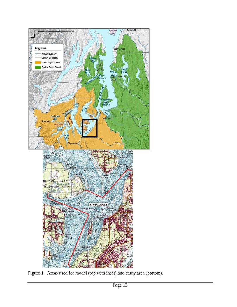
Description of Study Area South and Central Puget Sound include a complex and interconnected system of straits and open waters in Washington State. The northern border of South Puget Sound is defined traditionally by the Tacoma Narrows and an entrance sill located just to the south of the Tacoma Narrows. The sill is a shallow reach formed during the glacial epochs tens of thousands of years ago, with typical depths around 50 meters (m). Deeper regions to the west and landward of the sill are greater than 150 m. As shown in Figure 1, the study area stretches from north of Chambers Creek to Sequalitchew Creek in the south, and includes SE McNeil Island. It includes two major WWTPs: The Solo Point WWTP for JBLM and the Chambers Creek WWTP. Other major historical sources of pollution include particulate contamination from the former ASARCO plant, the Abitibi (formerly Boise Cascade) pulp mill facility, an armament factory in DuPont, JBLM activities, and the Steilacoom Marina.

Figure 1. Areas used for model (top with inset) and study area (bottom).

Computational Grid Development The current model grid was developed based on a previous model grid of South Puget Sound through Alki Point (Albertson et al., 2007). Given the potential for Central Puget Sound sources to impact South Puget Sound water quality, the model grid was extended northward to Edmonds. Each of the 2623 grid cells has a slightly different shape and surface area, but the nominal grid cell size is about 500 m x 500 m (Figure 2).

Figure 2. South and Central Puget Sound model grid. Long-term Ecology monitoring station GOR001 is indicated with a star. Depths for each model grid cell were determined by sampling the Finlayson (2005) digital elevation model. We re-projected the data from Washington State Plane North (feet) NAD83 to Washington State Plane South (feet) NAD83 HARN. We preserved the NAVD88 vertical datum from the original data. Using GIS, we used the model grid cell layer to define the spatial extent and averaged depth values within the 30-ft raster grid cells from the Finlayson (2005) combined

Hope Island

GOR001

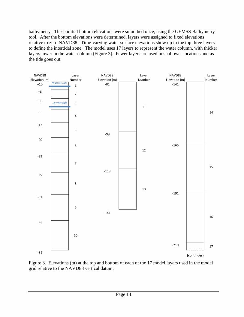
bathymetry. These initial bottom elevations were smoothed once, using the GEMSS Bathymetry tool. After the bottom elevations were determined, layers were assigned to fixed elevations relative to zero NAVD88. Time-varying water surface elevations show up in the top three layers to define the intertidal zone. The model uses 17 layers to represent the water column, with thicker layers lower in the water column (Figure 3). Fewer layers are used in shallower locations and as the tide goes out.

Figure 3. Elevations (m) at the top and bottom of each of the 17 model layers used in the model grid relative to the NAVD88 vertical datum.

NAVD88 Layer NAVD88 Layer NAVD88 LayerElevation (m) Number Elevation (m) Number Elevation (m) Number

-81(continues)

-141

-99

12

-119

13

-125

-165

15

-191

16

-219 17

-141

14

-81

11

8

9

10

-51

-39

-29

-20

1

2

3

4

6

7

+10

+6

+1

-5

-65

Highest tide

Lowest tide

The GEMSS model for South Puget Sound was calibrated and confirmed, using data collected from July through December 2006 (Roberts et al., 2014). Once a good fit to water surface elevations, temperature, and salinity was achieved, the model was compared to a second data set from January through October 2007 without adjusting calibrations parameters.

Boundary Conditions for 2012 This section presents the boundary conditions used at the northern seaward boundary, meteorology, and river and point source inflows. The subsequent section describes how we established initial conditions within the model domain to begin the simulation. Overall, the model performed well for 2012 as it did for 2006-7. 2012 was an unusual year, with cooler seawater temperatures that recovered in late autumn and higher precipitation and river flow that lowered salinity and density. Coastal upwelling was generally below expected median historic values but within expected historic ranges. Tidal Forcing Tidal forcing, expressed by changes in water surface elevations with time, results from the complex interaction of gravitational forces from the moon, sun, and the shape of marine waterbodies themselves. Astronomical tides also have a major effect on mixing processes in Puget Sound, followed in importance by wind-driven forcing, which is more important in shallower bays. The Puget Sound Tide Channel Model (PSTCM) predicts water surface elevations throughout Puget Sound based on the amplitude and phase of the full suite of tidal constituents (Lavelle et al., 1988; Mofjeld et al., 2002). Finlayson (2004) developed a stand-alone version of the updated PSTCM called PSTides. Tidal forcing at the open northern boundary, near Edmonds, was provided from PSTides. Correctly predicting water surface elevations is a key indicator that circulation models are calibrated correctly. We converted PSTides tidal elevations, expressed relative to mean lower low water (MLLW), to NAVD88 using the National Oceanic and Atmospheric Administration (NOAA) VDatum program (http://vdatum.noaa.gov/). All vertical elevations are expressed as NAVD88, Ecology’s standard datum, unless otherwise specified. Positive elevations indicate locations above the datum and negative elevations below it. The water surface elevation time series at PSTides segment 388 (see Model Calibration and Confirmation for location) was used as the northern boundary condition. In addition, we used PSTides to obtain water surface elevation for segment 182 (shown in Pacific Standard Time, PST) to compare with model output during model calibration and confirmation. Meteorological Forcing Meteorological forcing functions include precipitation, air and dew point temperatures, wind speed and direction, cloud cover, atmospheric pressure, relative humidity, and solar radiation. Meteorological stations used by the model were identical to those used in Roberts (2007). Puget Sound was fresher and generally cooler but less dense for much of 2012. By November’s dye

http://vdatum.noaa.gov/

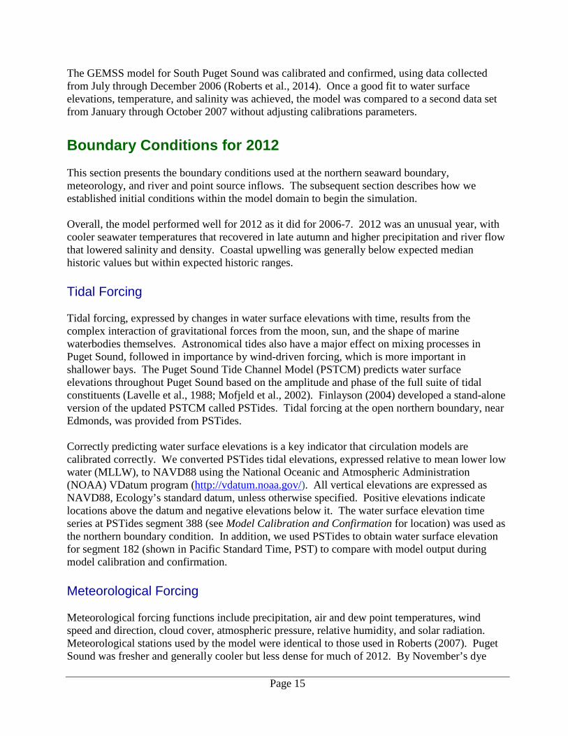
experiment, density and salinity in South Puget Sound were still significantly below normal against a 30-year average; however, water temperature rebounded to average after a warm October. Select meteorological conditions for 2012 are shown in Figure 4, and higher precipitation and cooler air temperatures are evident. a)

b)

c)

Figure 4. Meteorological conditions at SeaTac Airport for 2012 as (a) de-seasonalized anomalies (departure from 30-year daily averages) for air temperature, (b) precipitation (SeaTac and Shelton), and (c) cumulative precipitation at SeaTac.

Red fill shows surplus over normal rainfall, which is depicted by the lower smooth curve.

Rivers and Precipitation

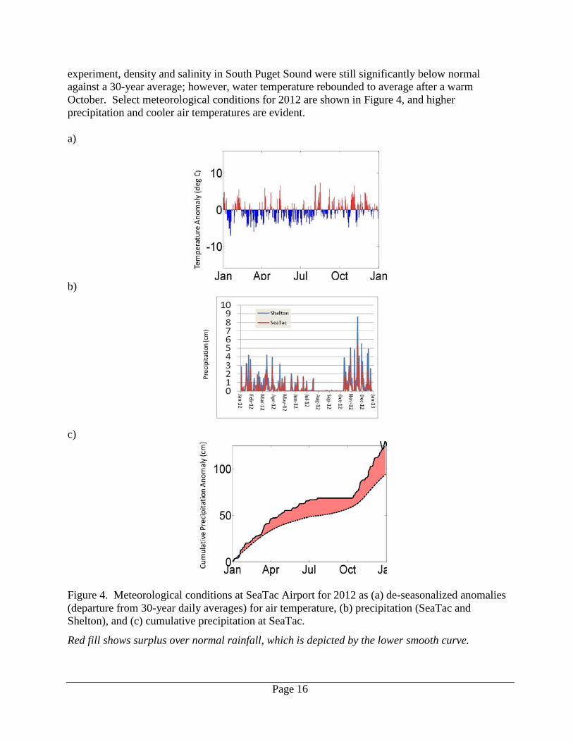
Figure 5. Watershed definitions used for freshwater inflows.

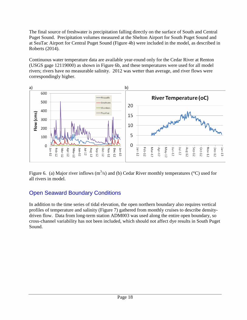
River inflow and precipitation were both abnormally high during 2012. During the dye experiment, salinity and density of Puget Sound were much lower than normal. The distribution of density with depth in Puget Sound is indicative of the estuarine flow that helps flush effluent and the dye plume seaward. Data on freshwater inflows from 66 rivers were compiled as described in Roberts et al. (2014). The major watersheds are shown in Figure 5. The most significant inflows for this study in 2012 are shown in Figure 6a. Freshwater inflows, including the shoreline areas not tributary to a major river or stream, were mapped to the surface layer of the grid cell nearest the discharge location, with the exception of Sinclair and Dyes Inlets. WWTPs also discharge freshwater to South and Central Puget Sound, although they represent <5% of the total freshwater inflows. For the purpose of this simulation, only JBLM and Chambers Creek WWTPs were included.

The final source of freshwater is precipitation falling directly on the surface of South and Central Puget Sound. Precipitation volumes measured at the Shelton Airport for South Puget Sound and at SeaTac Airport for Central Puget Sound (Figure 4b) were included in the model, as described in Roberts (2014). Continuous water temperature data are available year-round only for the Cedar River at Renton (USGS gage 12119000) as shown in Figure 6b, and these temperatures were used for all model rivers; rivers have no measurable salinity. 2012 was wetter than average, and river flows were correspondingly higher. a)

b)

Figure 6. (a) Major river inflows (m3/s) and (b) Cedar River monthly temperatures (°C) used for all rivers in model.

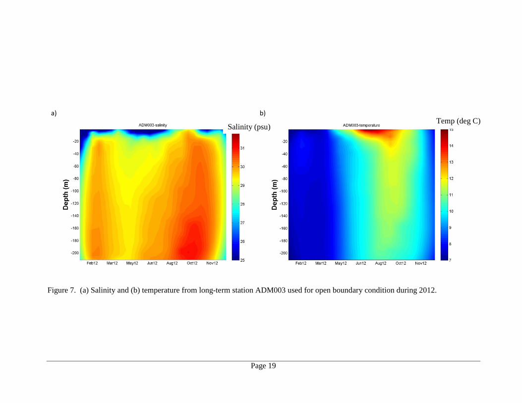
Open Seaward Boundary Conditions In addition to the time series of tidal elevation, the open northern boundary also requires vertical profiles of temperature and salinity (Figure 7) gathered from monthly cruises to describe density-driven flow. Data from long-term station ADM003 was used along the entire open boundary, so cross-channel variability has not been included, which should not affect dye results in South Puget Sound.

a)

b)

Figure 7. (a) Salinity and (b) temperature from long-term station ADM003 used for open boundary condition during 2012.

Salinity (psu)

Temp (deg C)

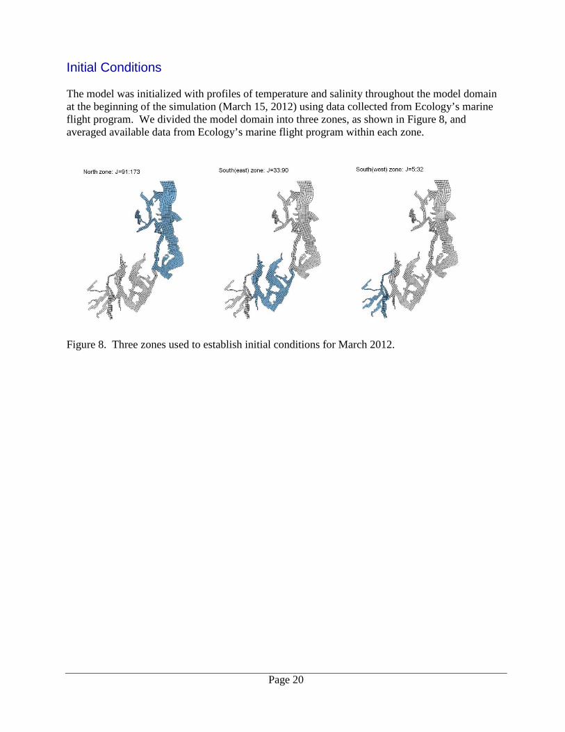
Initial Conditions The model was initialized with profiles of temperature and salinity throughout the model domain at the beginning of the simulation (March 15, 2012) using data collected from Ecology’s marine flight program. We divided the model domain into three zones, as shown in Figure 8, and averaged available data from Ecology’s marine flight program within each zone.

Figure 8. Three zones used to establish initial conditions for March 2012.

Model Calibration and Confirmation

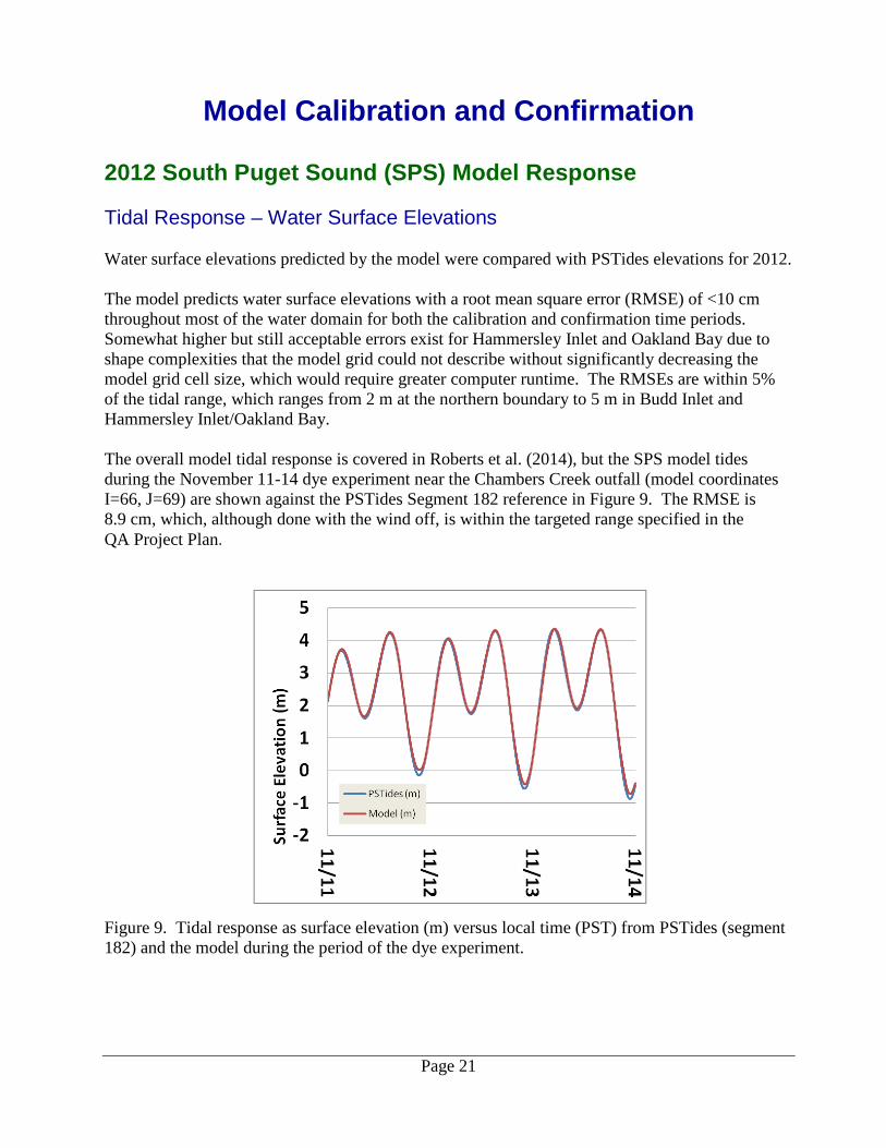
2012 South Puget Sound (SPS) Model Response Tidal Response – Water Surface Elevations Water surface elevations predicted by the model were compared with PSTides elevations for 2012. The model predicts water surface elevations with a root mean square error (RMSE) of <10 cm throughout most of the water domain for both the calibration and confirmation time periods. Somewhat higher but still acceptable errors exist for Hammersley Inlet and Oakland Bay due to shape complexities that the model grid could not describe without significantly decreasing the model grid cell size, which would require greater computer runtime. The RMSEs are within 5% of the tidal range, which ranges from 2 m at the northern boundary to 5 m in Budd Inlet and Hammersley Inlet/Oakland Bay. The overall model tidal response is covered in Roberts et al. (2014), but the SPS model tides during the November 11-14 dye experiment near the Chambers Creek outfall (model coordinates I=66, J=69) are shown against the PSTides Segment 182 reference in Figure 9. The RMSE is 8.9 cm, which, although done with the wind off, is within the targeted range specified in the QA Project Plan.

Figure 9. Tidal response as surface elevation (m) versus local time (PST) from PSTides (segment 182) and the model during the period of the dye experiment.

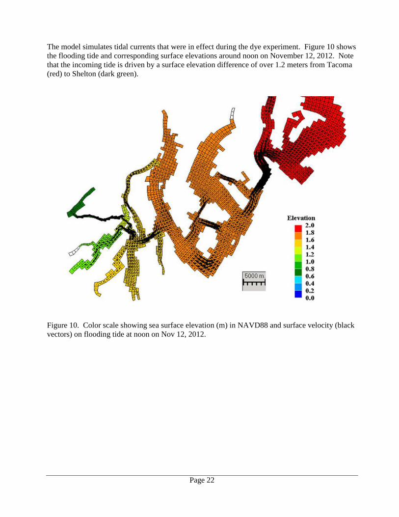
The model simulates tidal currents that were in effect during the dye experiment. Figure 10 shows the flooding tide and corresponding surface elevations around noon on November 12, 2012. Note that the incoming tide is driven by a surface elevation difference of over 1.2 meters from Tacoma (red) to Shelton (dark green).

Figure 10. Color scale showing sea surface elevation (m) in NAVD88 and surface velocity (black vectors) on flooding tide at noon on Nov 12, 2012.

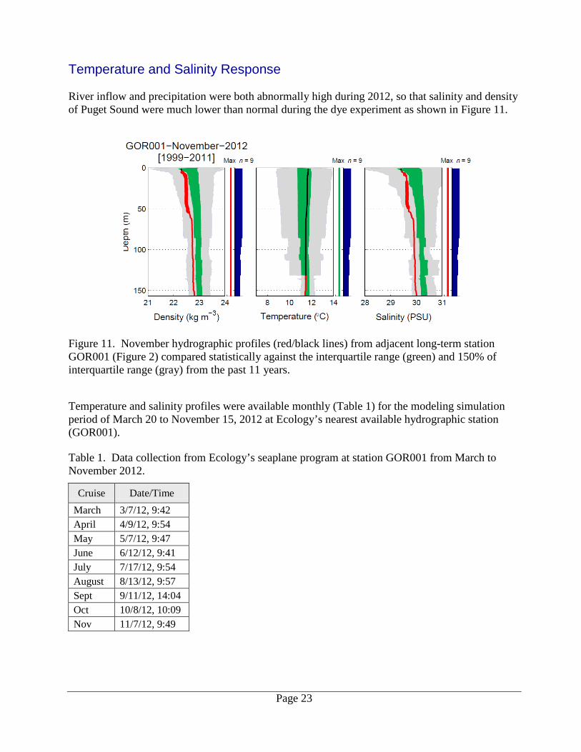
Temperature and Salinity Response River inflow and precipitation were both abnormally high during 2012, so that salinity and density of Puget Sound were much lower than normal during the dye experiment as shown in Figure 11.

Figure 11. November hydrographic profiles (red/black lines) from adjacent long-term station GOR001 (Figure 2) compared statistically against the interquartile range (green) and 150% of interquartile range (gray) from the past 11 years.

Temperature and salinity profiles were available monthly (Table 1) for the modeling simulation period of March 20 to November 15, 2012 at Ecology’s nearest available hydrographic station (GOR001).

Table 1. Data collection from Ecology’s seaplane program at station GOR001 from March to November 2012.

Cruise Date/Time March 3/7/12, 9:42 April 4/9/12, 9:54 May 5/7/12, 9:47 June 6/12/12, 9:41 July 7/17/12, 9:54 August 8/13/12, 9:57 Sept 9/11/12, 14:04 Oct 10/8/12, 10:09 Nov 11/7/12, 9:49

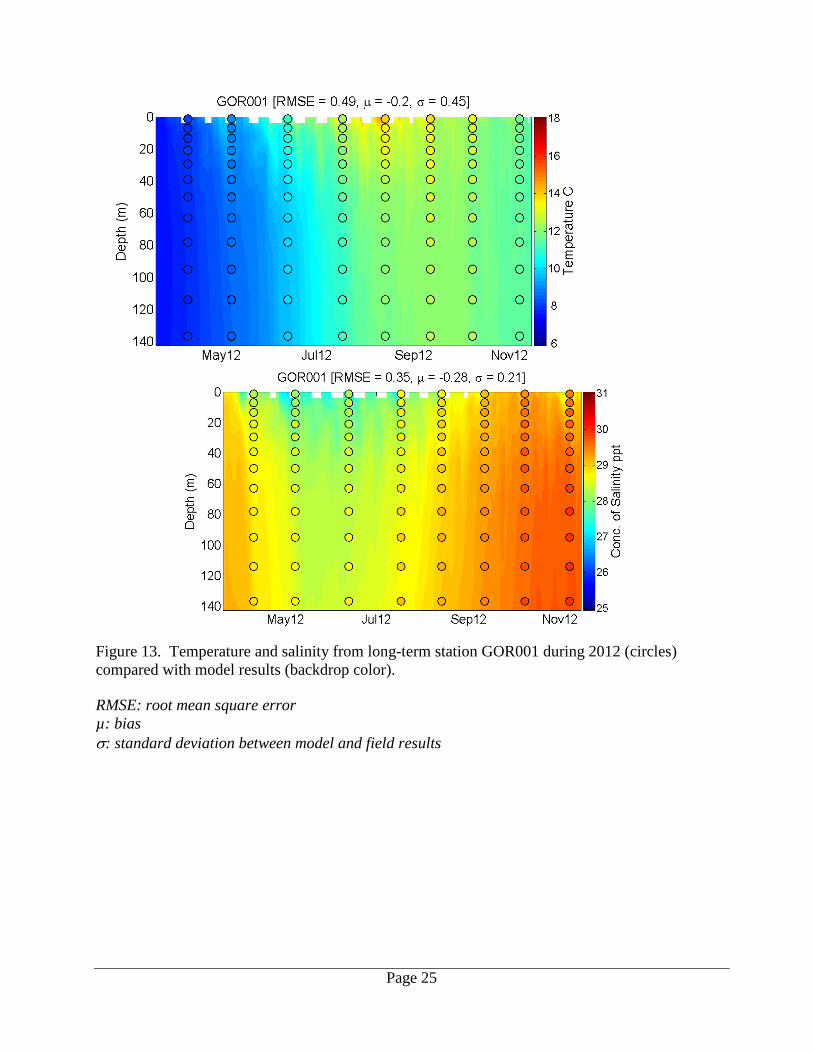
Observed data and the model simulation are compared in Figures 12 and 13. Figure 12 shows surface and bottom time series for the year and a vertical profile for the final data collection date shortly before the dye experiment. Figure 13 shows the field data with a colored circle. The colors outside of the circle show the model-simulated values. By comparing the two where they overlap, we can evaluate summary statistics. Temperature achieved an RMSE of 0.49 deg C with a bias of -0.2 deg C, and salinity had an RMSE of 0.35 psu with a bias of -0.28 psu over all available depth layers. The RMSE is within the target set forth in the QA Project Plan, and the bias is insignificant to the 95% confidence level (two standard deviations, which is 0.9 deg C for temperature and 0.42 psu for salinity). Date (2012)

Surface (KT) time series Bottom (KB) time series Nov 7 – vertical profiles

T

S

Figure 12. Temperature (T) and salinity (S) surface and bottom time series for model (solid line) and field (open circles) results as well as vertical profiles for the final survey date before the dye release experiment.

Figure 13. Temperature and salinity from long-term station GOR001 during 2012 (circles) compared with model results (backdrop color).

RMSE: root mean square error µ: bias σ: standard deviation between model and field results

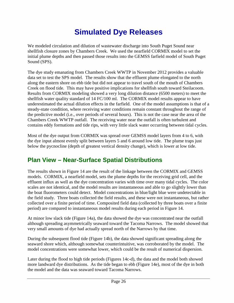
Simulated Dye Releases We modeled circulation and dilution of wastewater discharge into South Puget Sound near shellfish closure zones by Chambers Creek. We used the nearfield CORMIX model to set the initial plume depths and then passed those results into the GEMSS farfield model of South Puget Sound (SPS). The dye study emanating from Chambers Creek WWTP in November 2012 provides a valuable data set to test the SPS model. The results show that the effluent plume elongated to the north along the eastern shore on ebb tide but did not appear to travel south of the mouth of Chambers Creek on flood tide. This may have positive implications for shellfish south toward Steilacoom. Results from CORMIX modeling showed a very long dilution distance (6500 meters) to meet the shellfish water quality standard of 14 FC/100 ml. The CORMIX model results appear to have underestimated the actual dilution effects in the farfield. One of the model assumptions is that of a steady-state condition, where receiving water conditions remain constant throughout the range of the predictive model (i.e., over periods of several hours). This is not the case near the area of the Chambers Creek WWTP outfall. The receiving water near the outfall is often turbulent and contains eddy formations and tide rips, with very little slack water occurring between tidal cycles. Most of the dye output from CORMIX was spread over GEMSS model layers from 4 to 6, with the dye input almost evenly split between layers 5 and 6 around low tide. The plume traps just below the pycnocline (depth of greatest vertical density change), which is lower at low tide.

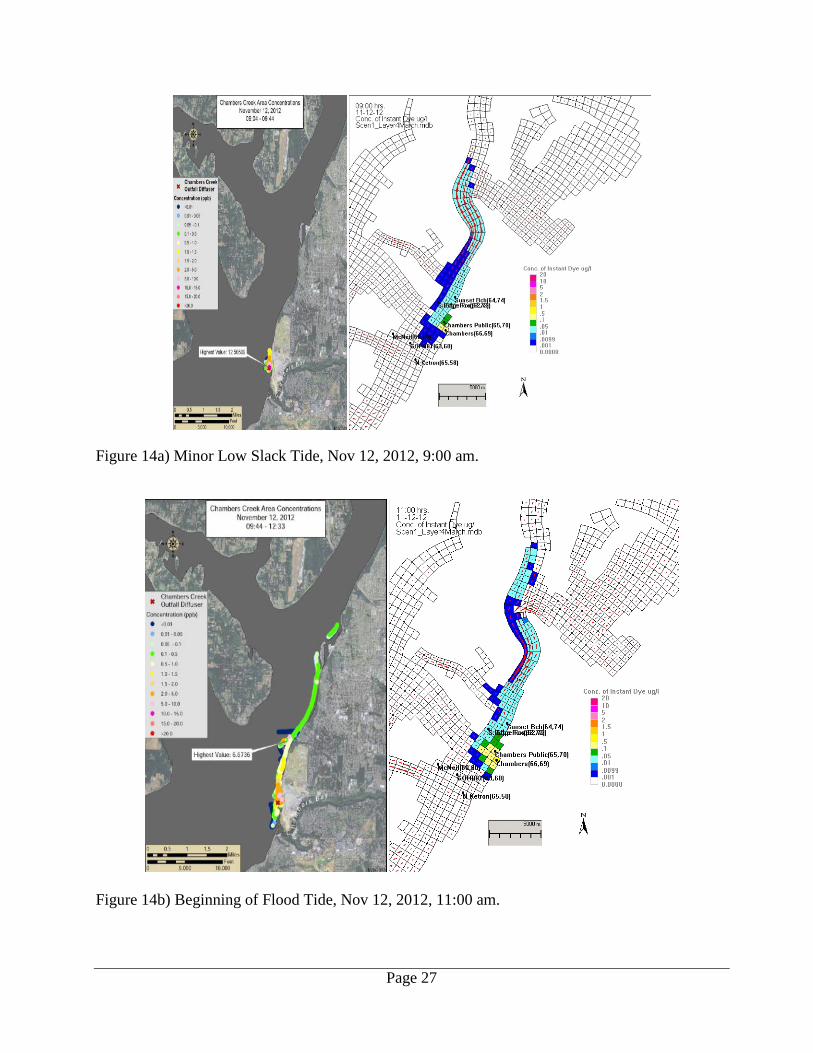
Plan View – Near-Surface Spatial Distributions The results shown in Figure 14 are the result of the linkage between the CORMIX and GEMSS models. CORMIX, a nearfield model, sets the plume depths for the receiving grid cell, and the effluent influx as well as the dye concentration varies with time over many tidal cycles. The color scales are not identical, and the model results are instantaneous and able to go slightly lower than the boat fluorometers could detect. Model concentrations in blue/light blue were undetectable in the field study. Three boats collected the field results, and these were not instantaneous, but rather collected over a finite period of time. Composited field data (collected by three boats over a finite period) are compared to instantaneous model results during each period in Figure 14.

At minor low slack tide (Figure 14a), the data showed the dye was concentrated near the outfall although spreading asymmetrically seaward toward the Tacoma Narrows. The model showed that very small amounts of dye had actually spread north of the Narrows by that time.

During the subsequent flood tide (Figure 14b), the data showed significant spreading along the seaward shore which, although somewhat counterintuitive, was corroborated by the model. The model concentrations were somewhat lower, which could be the result of numerical dispersion.

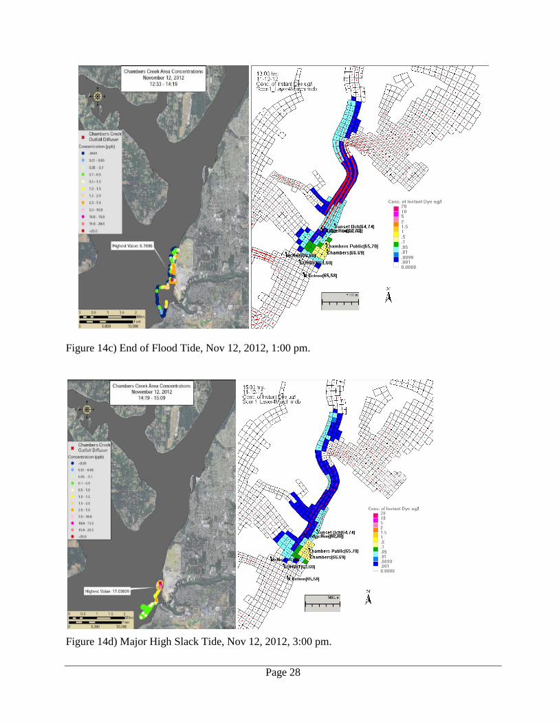
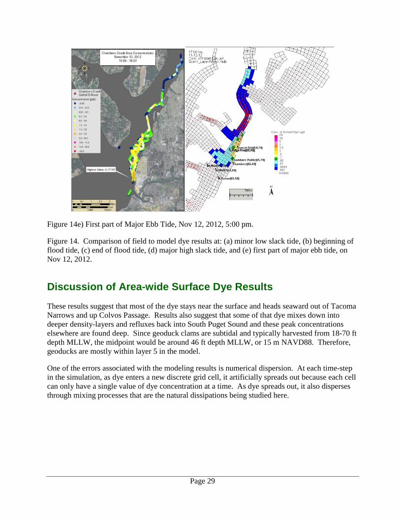
Later during the flood to high tide periods (Figures 14c-d), the data and the model both showed more landward dye distributions. As the tide began to ebb (Figure 14e), most of the dye in both the model and the data was seaward toward Tacoma Narrows.

Figure 14a) Minor Low Slack Tide, Nov 12, 2012, 9:00 am.

Figure 14b) Beginning of Flood Tide, Nov 12, 2012, 11:00 am.

Figure 14c) End of Flood Tide, Nov 12, 2012, 1:00 pm.

Figure 14d) Major High Slack Tide, Nov 12, 2012, 3:00 pm.

Figure 14e) First part of Major Ebb Tide, Nov 12, 2012, 5:00 pm.

Figure 14. Comparison of field to model dye results at: (a) minor low slack tide, (b) beginning of flood tide, (c) end of flood tide, (d) major high slack tide, and (e) first part of major ebb tide, on Nov 12, 2012.

Discussion of Area-wide Surface Dye Results These results suggest that most of the dye stays near the surface and heads seaward out of Tacoma Narrows and up Colvos Passage. Results also suggest that some of that dye mixes down into deeper density-layers and refluxes back into South Puget Sound and these peak concentrations elsewhere are found deep. Since geoduck clams are subtidal and typically harvested from 18-70 ft depth MLLW, the midpoint would be around 46 ft depth MLLW, or 15 m NAVD88. Therefore, geoducks are mostly within layer 5 in the model.

One of the errors associated with the modeling results is numerical dispersion. At each time-step in the simulation, as dye enters a new discrete grid cell, it artificially spreads out because each cell can only have a single value of dye concentration at a time. As dye spreads out, it also disperses through mixing processes that are the natural dissipations being studied here.

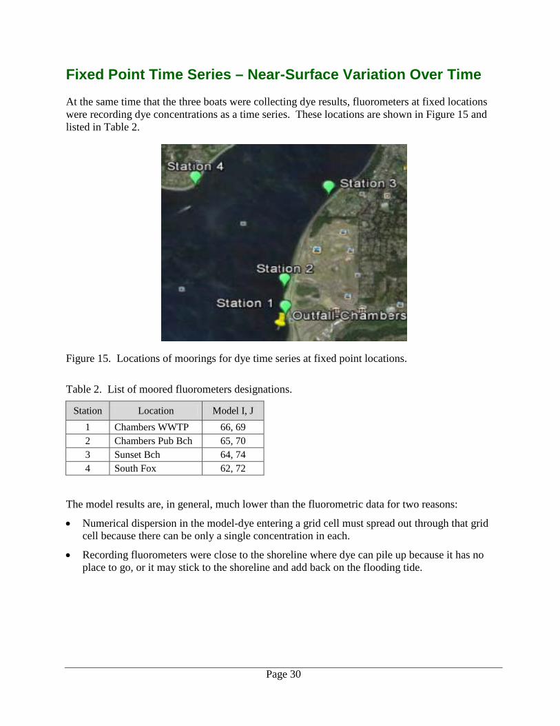
Fixed Point Time Series – Near-Surface Variation Over Time At the same time that the three boats were collecting dye results, fluorometers at fixed locations were recording dye concentrations as a time series. These locations are shown in Figure 15 and listed in Table 2.

Figure 15. Locations of moorings for dye time series at fixed point locations.

Table 2. List of moored fluorometers designations.

Station Location Model I, J 1 Chambers WWTP 66, 69 2 Chambers Pub Bch 65, 70 3 Sunset Bch 64, 74 4 South Fox 62, 72

The model results are, in general, much lower than the fluorometric data for two reasons:

• Numerical dispersion in the model-dye entering a grid cell must spread out through that grid cell because there can be only a single concentration in each.

• Recording fluorometers were close to the shoreline where dye can pile up because it has no place to go, or it may stick to the shoreline and add back on the flooding tide.

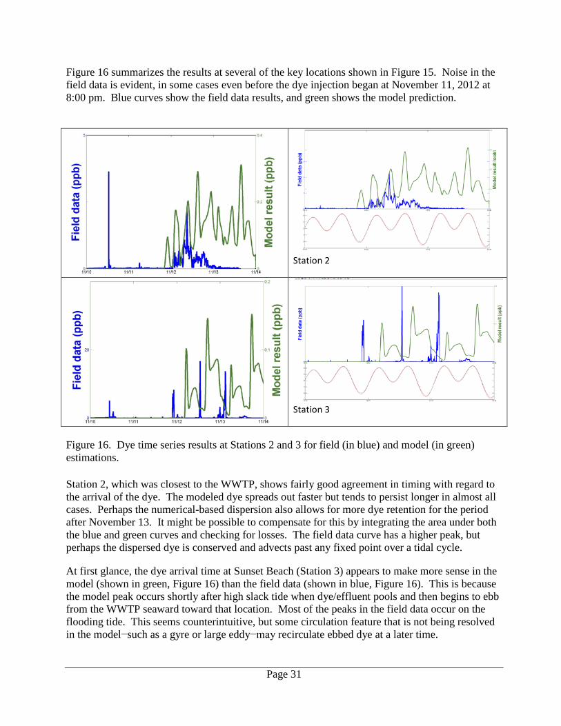
Figure 16 summarizes the results at several of the key locations shown in Figure 15. Noise in the field data is evident, in some cases even before the dye injection began at November 11, 2012 at 8:00 pm. Blue curves show the field data results, and green shows the model prediction.

Station 2

Station 3

Figure 16. Dye time series results at Stations 2 and 3 for field (in blue) and model (in green) estimations.

Station 2, which was closest to the WWTP, shows fairly good agreement in timing with regard to the arrival of the dye. The modeled dye spreads out faster but tends to persist longer in almost all cases. Perhaps the numerical-based dispersion also allows for more dye retention for the period after November 13. It might be possible to compensate for this by integrating the area under both the blue and green curves and checking for losses. The field data curve has a higher peak, but perhaps the dispersed dye is conserved and advects past any fixed point over a tidal cycle.

At first glance, the dye arrival time at Sunset Beach (Station 3) appears to make more sense in the model (shown in green, Figure 16) than the field data (shown in blue, Figure 16). This is because the model peak occurs shortly after high slack tide when dye/effluent pools and then begins to ebb from the WWTP seaward toward that location. Most of the peaks in the field data occur on the flooding tide. This seems counterintuitive, but some circulation feature that is not being resolved in the model−such as a gyre or large eddy−may recirculate ebbed dye at a later time.

It has been suggested that the offset in arrival time distinctly noticeable at Station 3 may be the result of a clockwise eddy that forms to the southeast of McNeil Island, as shown in Tide Prints (McGary and Lincoln, 1977). With a model grid size near 500 m, it is unlikely that such a feature would be reproduced in its entirety in the model. However, the model does predict higher dye concentration along the shoreline, which may partially be a result of this feature.

Numerical Dispersion Numerical dispersion occurs because each grid cell can have only a single value for dye concentration within it during a simulation. As dye enters a cell, it artificially spreads out to fill the entire cell, as it must, which in effect over-predicts dilution. The phenomenon gets worse with larger grid cells and with distance from the input location. One common modeling approach is to make models of varying grid cell size to determine at what resolution the problem can be ignored. This typically happens when grid cell size approaches the horizontal dimension of the plume. Since this model was created for Ecology, the grid size is inherent and difficult to change.

The approach used here is to estimate the numerical dispersion from the data results shown in Figure 16. Although there is no guarantee that the dye sensors detected the maximum value of dye, the amount of over-predicted dilution at any distance where there are data can be approximated by estimating the dye loss. By integrating the area under the concentration curve, it is possible to estimate numerical dispersion at several distances from the WWTP, by estimating dye losses to adjacent grid cells.

The field data are somewhat noisy, but the time-integral at Station 2 from 6:00 am to noon on November 12 evaluated to 79.7 ppb-min for the field results, and 42.0 ppb-min for the model (ratio of 1.9:1 at that distance, see map). At Station 3, integrating from November 12 at 8:00 pm to November 13 at noon, the field results were 486 ppb-min and the model was 86.2 ppb-min (ratio of 5.6:1 at roughly 4X the distance). Station 3 (Sunset Beach) was where there was more conversion of dye during the field study, which indicates there is something happening with circulation patterns that the model is not picking up. Ratio of field to modeled dilution at this station is much higher than at Station 2. Because this convergence effect is superimposed on the effects of numerical dispersion, the safety factor of 2 from Station 2 seems reasonable to use.

Dilution Ratios An alternate way of viewing the results shown earlier in Figure 14 is to calculate non-dimensional dilution ratios based on the initial concentration of dye divided by the concentration in any grid cell at any later time.

A 1000:1 dilution ratio is the minimum recommended by FDA for a prohibited area to account for viral impacts during normal operating conditions. This guidance is explained in Interstate Shellfish Sanitation Conference (ISSC) proposal 13-118 on page 186: www.issc.org/client_resources/2013%20biennial%20meeting/2013%20task%20force%20i/13-118.pdf. DOH sets the sanitary line based on the needed dilution to get to the shellfish standard assuming a loss of disinfection (most common upset condition).

http://www.issc.org/client_resources/2013%20biennial%20meeting/2013%20task%20force%20i/13-118.pdf

http://www.issc.org/client_resources/2013%20biennial%20meeting/2013%20task%20force%20i/13-118.pdf

Adjustments for the effect of numerical dispersion are to use the CORMIX model to set the concentrations in the grid cell that contains the discharge and then apply the safety factor calculated above. This report evaluates two scenarios: (1) the current as-built operating condition of 19 mgd, and (2) the future (~2035) build-out condition of 50 mgd.

Results for these two scenarios are presented in the following sequence:

• Map a shows the worst-case results just after low slack tide for the southern sanitary line. • Map b shows just after high slack tide for the northern line. • Map c shows the long-term steady-state after injecting dye for several months over all depths. • Map d shows the depth-layer at which the minimum value on map c occurred.

These results are shown at low tide, but tidal stage is less important at steady state.

Maps a and b show upset (transient) conditions rather than steady-state because dye was injected only for a single tidal cycle beforehand. Maps c and d result from five months of injection and are shown at low tide. True steady-state is achieved because the estimated flushing time of South Puget Sound is around two months. In all cases, the panels at far left in Figures 17 and 18 show the dye contours without accounting for numerical dispersion. The panels at far right use a safety factor of 2 for the contour lines display only. The safety factor of 2 is a modest attempt to compensate for the effects of numerical dispersion, as discussed in the previous section.

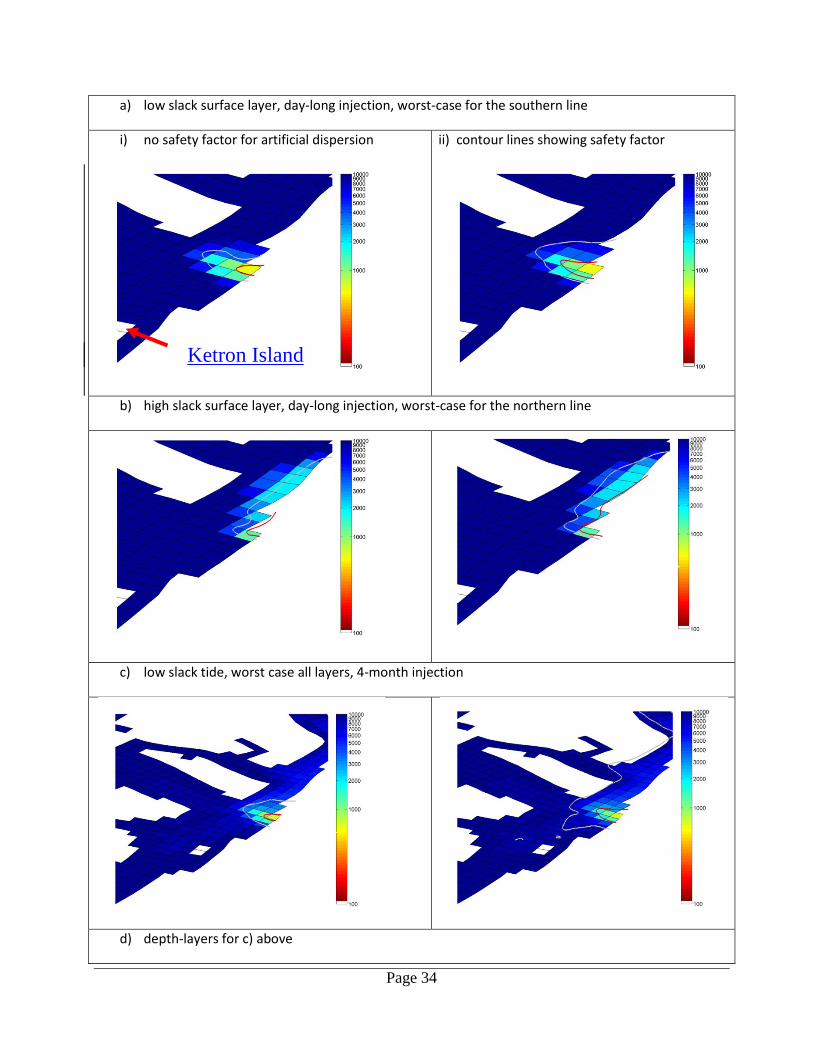
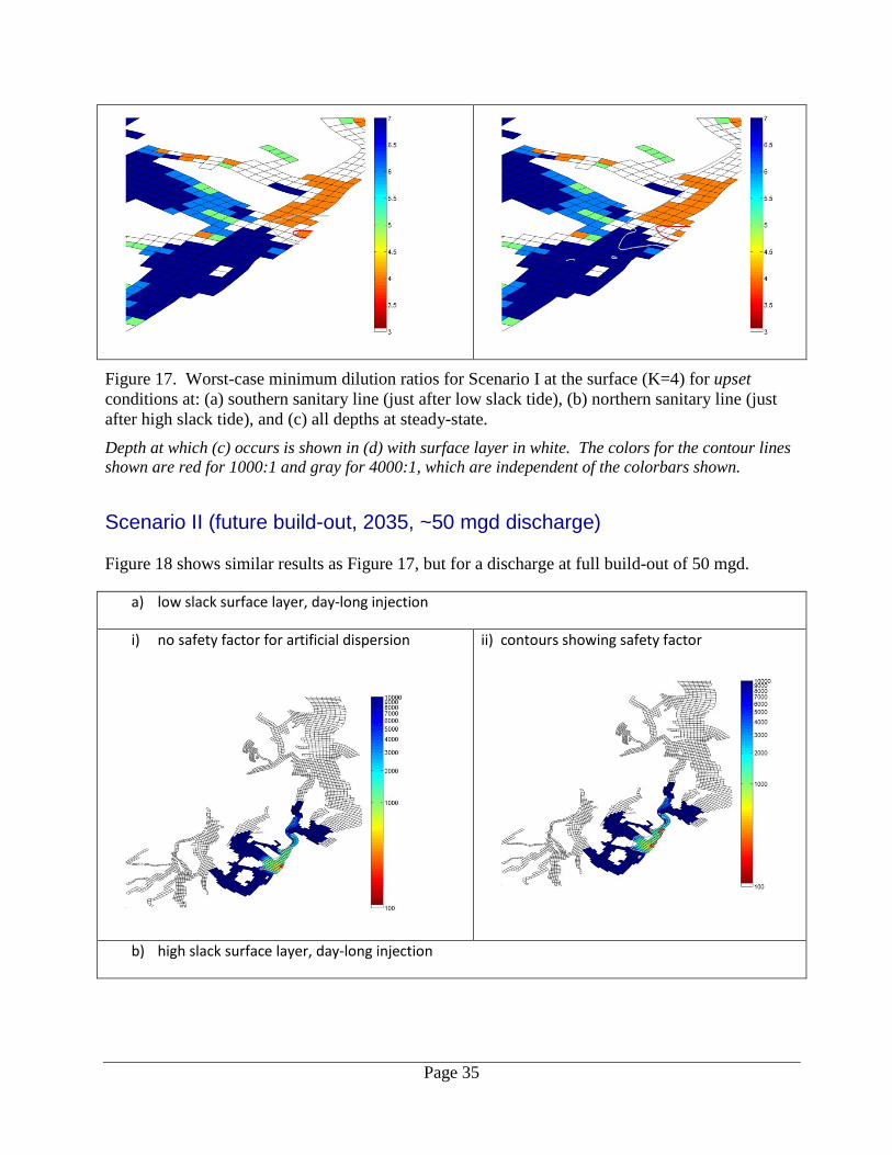
Scenario I (present ~19 mgd discharge) Figure 17a shows a close-up of the least diluted surface water ratios just after low slack tide (on November 12, 2012 at 11:00 am), worst-case to the south for effluent. The red contour shows the position of the 1000:1 dilution line, which is approximately where the sanitary line should be located. The gray line shows the 4000:1 dilution line, which is more conservative. Figure 17b shows results just after high slack tide (on November 12, 2012 at 5 pm), worst-case to the north for effluent. Note that the effluent still shows a prominent trail to the north at this tidal stage after hours of flooding tide. Figure 17c shows the maximum effluent concentrations / minimum dilution ratios over all depths at low slack tide. Figure 17d shows the depth at which those concentrations occur. Note that near the WWTP, which is where most of the field data were collected, the smallest dilutions occur near the surface (lighter color). At a distance from the WWTP, the depth with the lowest dilution is typically near-bottom, except in zones with lots of turbulence (e.g., Tacoma Narrows). The depths shown in Figure 17d are expressed as model layers; the larger the layer number, the deeper the result and the bluer the color.

a) low slack surface layer, day-long injection, worst-case for the southern line

i) no safety factor for artificial dispersion

ii) contour lines showing safety factor

b) high slack surface layer, day-long injection, worst-case for the northern line

c) low slack tide, worst case all layers, 4-month injection

d) depth-layers for c) above

Ketron Island

Figure 17. Worst-case minimum dilution ratios for Scenario I at the surface (K=4) for upset conditions at: (a) southern sanitary line (just after low slack tide), (b) northern sanitary line (just after high slack tide), and (c) all depths at steady-state. Depth at which (c) occurs is shown in (d) with surface layer in white. The colors for the contour lines shown are red for 1000:1 and gray for 4000:1, which are independent of the colorbars shown.

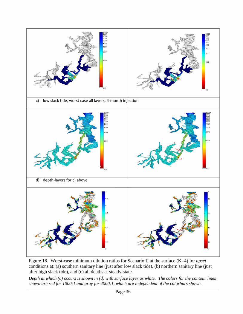
Scenario II (future build-out, 2035, ~50 mgd discharge) Figure 18 shows similar results as Figure 17, but for a discharge at full build-out of 50 mgd.

a) low slack surface layer, day-long injection

i) no safety factor for artificial dispersion

ii) contours showing safety factor

b) high slack surface layer, day-long injection

c) low slack tide, worst case all layers, 4-month injection

d) depth-layers for c) above

Figure 18. Worst-case minimum dilution ratios for Scenario II at the surface (K=4) for upset conditions at: (a) southern sanitary line (just after low slack tide), (b) northern sanitary line (just after high slack tide), and (c) all depths at steady-state. Depth at which (c) occurs is shown in (d) with surface layer as white. The colors for the contour lines shown are red for 1000:1 and gray for 4000:1, which are independent of the colorbars shown.

Conclusions and Recommendations The resolution of the South Puget Sound model is too coarse for nearfield simulations without CORMIX, and numerical dispersion makes the modeled dye dilutions greater than they should be. Nonetheless, the pattern of overall dispersal should be very useful to planners. Even with limitations imposed by resolution, this model is a better tool to evaluate sanitary lines than has been available previously.

The model confirms the observed net motion of WWTP effluent exiting north through Tacoma Narrows along the eastern shoreline and near the surface. Although results were not shown, this pattern occurs when the wind is absent as well. The refluxed dye modeled at depth contains very small concentrations of effluent, but effluent is present. That implies an expectation that discharge from Central Sound WWTPs, in general, will do likewise, since everything is interconnected. Perhaps this concern justifies Puget-Sound-wide planning and studies such as Roberts et al. (2014). Deep dye is below depths of geoducks, or it is so diluted that it should not pose a problem of and by itself. Fecal coliform bacteria counts decay with time, but model dye tracer lasts forever, in which case the deep effluent concentrations are conservative. Numerical dispersion is less important to these deep values because the time scale over which the artificial dispersion happens is so much less than the flushing time of South Puget Sound. After considering these modeling results and incorporating feedback from stakeholders, the Washington State Department of Health (DOH) will work with the Puget Sound Ecosystem Monitoring Program (PSEMP) to improve environmental modeling through incorporating DOH dye study and nearshore water quality monitoring results to calibrate and refine the models. These better models, in turn, would provide better information on which DOH can make shellfish harvest management decisions.

References Ahmed, A., G. Pelletier, M. Roberts, and A. Kolosseus, 2014. South Puget Sound Dissolved Oxygen Study: Water Quality Model Calibration and Scenarios. Washington State Department of Ecology, Olympia, WA. Publication No. 14-03-004. https://fortress.wa.gov/ecy/publications/SummaryPages/1403004.html Albertson, S., 2004. Oakland Bay Study: A dye and modeling study in an enclosed estuary with a high degree of refluxing. Washington State Department of Ecology, Olympia, WA. Publication No. 04-03-020. https://fortress.wa.gov/ecy/publications/SummaryPages/0403020.html Albertson, S., J. Bos, K. Erickson, C. Maloy, G. Pelletier, and M. Roberts, 2007. Quality Assurance Project Plan: South Puget Sound Water Quality Study Phase 2: Dissolved Oxygen. Washington State Department of Ecology, Olympia, WA. Publication No. 07-03-101. https://fortress.wa.gov/ecy/publications/SummaryPages/0703101.html Albertson, S., 2013. Addendum to Quality Assurance Project Plan: South Puget Sound Water Quality Study Phase 2: Dissolved Oxygen for Evaluation of Shellfish Harvesting near Joint Base Lewis-McChord and Chambers Creek. Washington State Department of Ecology, Olympia, WA. Publication No. 13-03-102. https://fortress.wa.gov/ecy/publications/SummaryPages/1303102.html Aura Nova Consultants, Brown and Caldwell, Inc., Evans-Hamilton, Inc., J.E. Edinger and Associates, Washington State Department of Ecology, and A. Devol, University of Washington Department of Oceanography, 1998. Budd Inlet Scientific Study Final Report. Prepared for Lacey, Olympia, Tumwater, Thurston Alliance (LOTT) Wastewater Management District. 300 pp. Cole, T.M. and E.M. Buchak, 1995. CE-QUAL-W2: A Two-Dimensional, Laterally Averaged, Hydrodynamic and Water Quality Model, Version 2.0: Users Manual, Instruction Report EL-95-1. US Army Engineer Waterways Experiment Station, Vicksburg, MS. Doneker, R.L. and G.H. Jirka, 1991. Expert Systems for Mixing Zone Analysis and Design of Aqueous Pollutant Discharges. Journal of Water Resources Planning and Management, ASCE Vol 117, No. 6, November/December 1991. Edinger, J.E. and E.M. Buchak, 1980. Numerical Hydrodynamics of Estuaries in. Estuarine and Wetland Processes with Emphasis on Modeling. Edinger, J.E. and E.M. Buchak, 1995. Numerical Intermediate and Far Field Dilution Modeling. Journal of Water, Air and Soil Pollution 83: 147-160, 1995. Finlayson, D.P., 2004. Puget Sound Tide Model (PSTides). www.ecy.wa.gov/programs/eap/models.html


https://fortress.wa.gov/ecy/publications/summarypages/0403020.html



http://www.ecy.wa.gov/programs/eap/models.html

Finlayson, D.P., 2005. Combined bathymetry and topography of the Puget Lowland, Washington State. University of Washington, Seattle, WA. www.ocean.washington.edu/data/pugetsound/ Kolluru, V.S., E.M. Buchak, and J.E. Edinger, 1998. Integrated Model to Simulate the Transport and Fate of Mine Tailings in Deep Waters. In Proceedings of Tailings and Mine Waste ’98. 1998. Balkema, Rotterdam, ISBN 905410922. Lavelle, J.W., H.O. Mofjeld, E. Lempriere-Doggett, G.A. Cannon, D.J. Pashinski, E.D. Cokelet, L. Lytle, and S. Gill, 1988. A Multiply-Connected Channel Model of Tides and Tidal Currents in Puget Sound, Washington and a Comparison with Update Observations. NOAA Technical Memorandum ERL PMEL-84. McGary, N. and J.H. Lincoln, 1977. Tide prints: Surface currents in Puget Sound. Washington Sea Grant Publication Number WSG 77-1. Mofjeld, H.O., A.J. Venturato, V.V. Titov, F.I. González, and J.C. Newman, 2002. Tidal Datum Distributions in Puget Sound, Washington, Based on a Tidal Model. NOAA Technical Memorandum OAR PMEL-122 (PB2003102259). NOAA/Pacific Marine Environmental Laboratory, Seattle, WA. 35 pp. National Shellfish Sanitation Program (NSSP), 2011. Guide for the Control of Molluscan Shellfish. www.fda.gov/downloads/Food/GuidanceRegulation/FederalStateFoodPrograms/UCM350344.pdf Roberts, M. 2007. Addendum to the Quality Assurance Project Plan for the South Puget Sound Water Quality Study, Phase 2: Dissolved Oxygen. Washington State Department of Ecology, Olympia, WA. Publication No. 07-03-101ADD1. https://fortress.wa.gov/ecy/publications/SummaryPages/0703101add1.html Roberts, M.L., A. Ahmed, and G. Pelletier, 2012. Deschutes River, Capitol Lake, and Budd Inlet Temperature, Fecal Coliform Bacteria, Dissolved Oxygen, pH, and Fine Sediment Total Maximum Daily Load Technical Report: Water Quality Study Findings. Washington State Department of Ecology, Olympia, WA. Publication No. 12-03-008. https://fortress.wa.gov/ecy/publications/SummaryPages/1203008.html Roberts, M., S. Albertson, A. Ahmed, and G. Pelletier, 2014. South Puget Sound Dissolved Oxygen Study: South and Central Puget Sound Water Circulation Model Development and Calibration. Washington State Department of Ecology, Olympia, WA. Publication No. 14-03-015. https://fortress.wa.gov/ecy/publications/SummaryPages/1403015.html Toy, M., 2011. Quality Assurance Project Plan: Restore Shellfish Harvesting to Joint Base Lewis-McChord/Chambers Creek Prohibited Area (EPA Cooperative Agreement PC-00J28001). Washington State Department of Health, Olympia, WA.

http://www.ocean.washington.edu/data/pugetsound/

http://www.fda.gov/downloads/Food/GuidanceRegulation/FederalStateFoodPrograms/UCM350344.pdf

https://fortress.wa.gov/ecy/publications/SummaryPages/0703101add1.html



Appendix. Glossary, Acronyms, and Abbreviations

Glossary Dissolved oxygen: A measure of the amount of oxygen dissolved in water.

Parameter: Water quality constituent being measured (analyte). A physical, chemical, or biological property whose values determine environmental characteristics or behavior.

Point source: Sources of pollution that discharge at a specific location from pipes, outfalls, and conveyance channels to a surface water. Examples of point source discharges include municipal wastewater treatment plants, municipal stormwater systems, industrial waste treatment facilities, and construction sites that clear more than 5 acres of land.

Watershed: A drainage area or basin in which all land and water areas drain or flow toward a central collector such as a stream, river, or lake at a lower elevation.

Acronyms and Abbreviations

DNR Department of Natural Resources DOH Washington State Department of Health Ecology Washington State Department of Ecology EPA U.S. Environmental Protection Agency FC Fecal coliform bacteria FDA U.S. Food and Drug Administration GEMSS Generalized Environmental Modeling System for Surfacewaters (model) GIS Geographic Information System JBLM Joint Base Lewis-McChord LOTT Lacey, Olympia, Tumwater, and Thurston County wastewater agency MLLW Mean lower low water NAVD88 North American Vertical Datum of 1988 NOAA National Oceanic and Atmospheric Administration NSSP National Shellfish Sanitation Program PST Pacific Standard Time PSTCM Puget Sound Tide Channel Model QA Quality Assurance RMSE Root mean square error SPS South Puget Sound USGS U.S. Geological Survey WAC Washington Administration Code WRIA Water Resource Inventory Area WWTP Wastewater Treatment Plant

Units of Measurement deg C degrees centigrade cm centimeter m meter mgd million gallons per day ml milliliters ppb parts per billion psu practical salinity units

chambers creek dye study: final model simulation report · chambers creek . dye study . final model...

Documents