ISSN 2042-2695

CEP Discussion Paper No 1077

September 2011

Stock Market Volatility and Learning

Klaus Adam, Albert Marcet and Juan Pablo Nicolini

Abstract We study a standard consumption based asset pricing model with rationally investing agents but allow

agents’ prior beliefs about price and dividend behavior to deviate slightly from rational expectations

priors. Learning about stock price behavior then causes the model to become quantitatively consistent

with a range of basic asset prizing ‘puzzles’: stock returns display momentum and mean reversion,

asset prices become volatile, the price-dividend ratio displays persistence, long-horizon returns

become predictable and a risk premium emerges. Comparing the moments of the model with those in

the data using confidence bands from the method of simulated moments, we show that our findings

are robust to different assumptions on the system of beliefs and other model features. We depart from

previous studies of asset prices under learning in that agents form expectations about future stock

prices using past price observations.

JEL Classifications: G12, D84

Keywords: asset pricing, learning, near-rational price forecasts

This paper was produced as part of the Centre’s Macro Programme. The Centre for Economic

Performance is financed by the Economic and Social Research Council.

Acknowledgements Thanks go to Davide Debortoli, Luca Dedola, George Evans, Katharina Greulich, Seppo Honkapohja,

Ricardo Lagos, Erzo Luttmer, Bruce McGough, Bruce Preston, Jaume Ventura, Joachim Voth, Iván

Werning and Raf Wouters for interesting comments and suggestions. We particularly thank Philippe

Weil for a very interesting and stimulating discussion. Sofía Bauducco and Davide Debortoli have

supported us with outstanding research assistance. Marcet acknowledges support from CIRIT

(Generalitat de Catalunya), Plan Nacional project ECO2008- 04785/ECON (Ministry of Science and

Education, Spain), CREI, the Barcelona GSE Research Network and the Wim Duisenberg fellowship

from the European Central Bank. The views expressed herein are solely those of the authors and do

not necessarily reflect the views of the Federal Reserve Bank of Minneapolis or the Federal Reserve

System.

Klaus Adam is Professor of Economics at Mannheim University. Albert Marcet is an

Associate of the Macro Programme at the Centre for Economic Performance and Lecturer in

Economics, London School of Economics. Juan Pablo Nicolini is a Senior Economist with The

Federal Reserve Bank of Minneapolis and Professor of Economics, currently on sabbatical from the

Universidad Di Tella.

Published by

Centre for Economic Performance

London School of Economics and Political Science

Houghton Street

London WC2A 2AE

All rights reserved. No part of this publication may be reproduced, stored in a retrieval system or

transmitted in any form or by any means without the prior permission in writing of the publisher nor

be issued to the public or circulated in any form other than that in which it is published.

Requests for permission to reproduce any article or part of the Working Paper should be sent to the

editor at the above address.

K. Adam, A. Marcet and J. P. Nicolini, submitted 2011

"Investors, their confidence and expectations buoyed by past priceincreases, bid up speculative prices further, thereby enticing moreinvestors to do the same, so that the cycle repeats again and again.”

Irrational Exuberance, Shiller (2005, p.56)

1 Introduction

The purpose of this paper is to show that a very simple asset pricing modelis able to quantitatively reproduce a variety of stylized asset pricing facts ifone allows for small departures from rational expectations.

We study a simple variant of Lucas (1978) model. It is well known thatthe asset prices implications of this model under rational expectations (RE)are at odds with some basic facts: in the data, the price dividend ratio istoo volatile and persistent, stock returns are too volatile, long horizon excessreturns of stocks are negatively related to the price dividend ratio, and therisk premium is too high. We stick to Lucas’ framework but allow for agentswhose prior beliefs about price and dividend behavior deviate slightly fromthose assumed under a rational expectations (RE) analysis of the model.Our slight relaxation of prior beliefs implies that agents need to learn aboutstock price behavior and we show that this feature alters the asset pricepredictions of the model in a way to make it quantitatively consistent withall the basic facts listed above.

We consider investors who hold a consistent system of beliefs about thestochastic process for payoff-relevant variables that are beyond their control.In our model, these variables consist of the (exogenous) dividend process andthe process for (competitive) stock market prices. And given these beliefsinvestors maximize a standard time-separable utility function subject totheir budget constraints. We call such agents ‘internally rational’. Justto emphasize: such agents behave as if they knew dynamic programmingunder uncertainty, the theory of Markov stochastic processes and Bayesianupdating and filtering.

Unlike in a RE analysis, however, we do not assume that agents knowperfectly how a certain dividend history maps into a market outcome for thestock price.1 Agents express this uncertainty by specifying a subjective dis-

1Such uncertainty may arise from a lack of common knowledge of investors’ price anddividend beliefs, as is explained in detail in Adam and Marcet (forthcoming).

1

tribution over stock price and dividend outcomes and optimally update theirbeliefs about price behavior in the light of realized market outcomes. Fora general class of beliefs, we find that such learning from market outcomesimparts ‘momentum’ on stock prices and produces large and sustained de-viations of the price dividend ratio from its mean, as can be observed in thedata. Such momentum arises because if agents’ expectations about stockprice growth increase in a given period, the actual growth rate of prices hasa tendency to increase beyond the fundamental growth rate, thereby rein-forcing the initial belief of higher stock price growth. Yet, the model alsodisplays ‘mean reversion’ so that so that even if expectations are very highor very low at some point, they will eventually return to fundamentals. Themodel thus displays something like the ‘naturally occurring Ponzi schemes’described in the opening quote.

Our formulation of beliefs naturally nests RE as a special case and there-fore provides a precise sense in which beliefs are close to the RE prior beliefs.To capture the distance relative to the RE prior we add just one free pa-rameter relative to the standard model and this parameter has a naturaleconomic and statistical interpretation capturing the strength with whichagents’ beliefs react to market outcomes. Under the RE analysis, marketoutcomes carry only redundant information, so that this parameter is set tozero. But as we document, the match with the data becomes very good forbelief systems that imply that agents should place a small but strictly posi-tive weight on market information. We find it a striking observation that theasset pricing implications of the standard model are not robust to such smalldepartures from rational price expectations and that this non-robustness isempirically so encouraging. This suggests that allowing for such kind ofdepartures from a strong assumption (RE) could be a promising avenue forresearch more generally.

We wish to emphasize that we achieve the fit with the data within a verysimple setting. The asset pricing equation derived in the paper is the sameone-step-ahead equation that is typically considered under the RE analysisof the model. Moreover, internally rational behavior implies that agents usea standard model of adaptive learning to update their subjective expecta-tions of the one-step-ahead variables appearing in the asset pricing equation.Specifically, Bayesian belief updating implies that agents optimally use leastsquares learning, and as we show, agents would asymptotically converge tothe RE outcome, i.e., learn to become fully rational, although this takesa long time. To avoid the issue of asymptotically vanishing volatility andto obtain an ergodic equilibrium distribution, we focus in our empiricalapplication mainly on a constant gain learning mechanism, which places

2

non-vanishing weight on market information.The paper is organized as follows. In section 2 we discuss the related

literature and section 3 presents the stylized asset pricing facts we seek tomatch. In section 4 we then outline the asset pricing model and derive aseries of analytic results for the case with risk neutral investors to show howour model is able to qualitatively deliver the stylized asset pricing facts fora general class of belief systems. In section 5 we present the baseline assetpricing model with risk aversion used in our empirical application and thebaseline calibration procedure for matching the data. Section 6 shows thatthe baseline model can quantitatively reproduce the facts discussed in section3 and also documents the robustness of our findings to various assumptionsabout the model or the estimation procedure.

Readers interested in obtaining a glimpse of the quantitative performanceof our one parameter extension of the RE model may directly jump to Table2 in section 6.1.

2 Related Literature

A large body of literature has documented that the basic asset pricing modelwith time separable preferences and RE has great difficulties in matching thevolatility and persistence of the price dividend ratio, the volatility of stockreturns, the predictability of excess returns at long horizons and the riskpremium.2 Models of learning have for long been considered as a promisingavenue for increasing the model implied volatility and thereby the matchwith the data.

A string of papers within the adaptive learning literature study agentswho learn about stock prices. Bullard and Duffy (2001) and Brock andHommes (1998) show that learning dynamics can converge to complicatedattractors and that the RE equilibrium may be unstable under learningdynamics.3 Branch and Evans (forthcoming) study a model where agents’algorithm to form expectations switches depending on which of the availableforecast models is performing best. Marcet and Sargent (1992) also studyconvergence to RE in a model where agents use today’s price to forecastthe price tomorrow in a stationary environment with private information.Cárceles-Poveda and Giannitsarou (2007) assume that agents know the mean

2See Cambell (2003) for an overview. Cecchetti, Lam, and Mark (2000) determine themisspecification in beliefs about future consumption growth required to match the equitypremium and other moments of asset prices.

3Stability under learning dynamics is defined in Marcet and Sargent (1989).

3

stock price and find that learning does then not significantly alter the be-havior of asset prices. Relative to these papers we address the data moreclosely and we derive our model of adaptive learning and asset pricing frominternally rational investor behavior.

Stock price behavior under Bayesian learning has been previously studiedin Timmermann (1993, 1996), Brennan and Xia (2001), Cogley and Sargent(2008) and Pastor and Veronesi (2003) among others. Agents in these paperslearn about the dividend process and then set the asset price equal to the dis-counted expected sum of dividends. This amounts to assuming that agents’beliefs about the joint distribution of prices and dividends contains a singu-larity and that market outcomes contain only redundant information. As aresult, there is no feedback from market outcomes (stock prices) to beliefs(price expectations). Agents’ beliefs in these settings are thus ‘anchored’by the exogenous dividend process, so that the volatility effects resultingfrom learning are generally limited when considering standard time separa-ble preference specifications. In contrast, we largely abstract from learningabout the dividend process and consider learning about stock price behaviorusing past price observations. In such a setting price beliefs and actual priceoutcomes mutually influence each other. It is precisely this self-referentialnature of the learning problem that imparts momentum to expectations andis key in explaining stock price volatility.4

In contrast to the RE literature, the behavioral finance literature tries tounderstand the decision-making process of individual investors by means ofsurveys, experiments and micro evidence, exploring the intersection betweeneconomics and psychology, see Shiller (2005) for a non-technical summary.We borrow from this literature an interest in deviating from RE but we areinterested in small deviations from the standard approach: we assume thatagents behave optimally given a consistent system of subjective beliefs thatare close to RE beliefs.

3 Facts

This section describes stylized facts of U.S. stock price data that we seek toreplicate in our quantitative analysis. These observations have been exten-sively documented in the literature. We reproduce them here as a point of

4Timmerman (1996) also analyzes a case with self-referential learning, assuming thatagents use dividends to predict future price. He reports that this form of learning deliverseven lower volatility than a settings with learning about the dividend process only. It isthus crucial for our results that agents use information on past price behavior to predictfuture price behavior.

4

0

100

200

300

400

1925 1930 1935 1940 1945 1950 1955 1960 1965 1970 1975 1980 1985 1990 1995 2000 2005

Figure 1: Quarterly U.S. price dividend ratio 1927:1-2005:4

reference using a single and updated data base.5

Since the work of Shiller (1981) and LeRoy and Porter (1981) it has beenrecognized that the volatility of stock prices in the data is much higher thanstandard RE asset pricing models suggest, given the available evidence onthe volatility of dividends. Figure 1 shows the evolution of the quarterlyprice dividend (PD) ratio in the United States. The PD ratio displays verylarge fluctuations around its sample mean (the green horizontal line in thegraph): in the year 1932, for example, the PD ratio takes on values below30, while in the year 2000 values close to 350. The standard deviation of thePD ratio (σPD) is almost one half of its sample mean (E(PD)). We reportthis feature of the data as Fact 1 in Table 1.

Figure 1 also shows that the deviation of the PD ratio from its samplemean are very persistent, so that the first order quarterly autocorrelationof the PD ratio (ρPD,−1) is very high. We report this as Fact 2 in Table 1below .

Related to the excessive volatility of prices is the observation that thevolatility of stock returns (σrs) in the data is almost four times the volatilityof dividend growth (σ∆D/D). We report the volatility of returns as Fact 3in Table 1, and the mean and standard deviation of dividend growth at the

5Details on the data sources are provided in Appendix 8.1.

5

bottom of the table.6

U.S. asset pricing facts, 1927:2-2005:4(quarterly real values, growth rates & returns in percentage terms)

Fact 1 Volatility of E(PD) 113.20PD ratio σPD 52.98

Fact 2 Persistence of ρPD,−1 0.92PD ratio

Fact 3 Excessive return σrs 11.65volatility

Fact 4 Excess return c25 -0.0048predictability R25 0.1986

Fact 5 Equity premium E [rs] 2.41E£rb¤

0.18

Dividend Mean Growth E¡∆DD

¢0.0035

Behavior Std of Growth σ∆DD

2.98

Table 1: Stylized asset pricing facts

While stock returns are difficult to predict at short horizons, the PDratio helps to predict future excess stock returns in the long run. Moreprecisely, estimating the regression

Xt,n = c1n + c2n PDt + ut,n

where Xt,n is the observed real excess return of stocks over bonds fromquarter t to quarter t plus n years, and ut,n the regression residual, theestimate c2n is found to be negative, significantly different from zero, and

6We treat the dividend process as exogenous in the model, therefore do not report thedividend moments as ‘Facts’ that have to be matched endogenously by our model.

6

the absolute value of c2n and the R-square of this regression, denoted R2n,increase with n. We choose to include the OLS regression results for the5-year horizon as Fact 4 in Table 1.7

Finally, it is well known that through the lens of standard models realstock returns tend to be too high relative to short-term real bond returns.This so called equity premium puzzle is reported as Fact 5 in Table 1, whichshows that the average quarterly real return on bonds E

¡rbt¢is much lower

than the corresponding return on stocks E (rst ) .Table 1 reports ten statistics. As we show in section 6, once we use the

evidence on dividend growth to calibrate the dividend process in the model,we can replicate the remaining 8 statistics listed as Facts 1-5 using a modelthat has only two free parameters.

4 The Theory

We describe in section 4.1 below a basic Lucas (1978) asset pricing modelwith internally rational agents and derive the resulting asset pricing equa-tion when agents are uncertain about the price outcomes. Section 4.2 thenpresents - for the case with risk neutral investors - a number of analytical re-sults regarding asset price behavior under learning. These results illustratewhy our learning model can qualitatively replicate the facts mentioned inTable 1 for a large number of natural belief specifications. Finally, section4.3 shows how internally rational behavior is compatible with well knownmodels of adaptive learning.

4.1 The Model

The Environment: Consider an economy populated by a unit mass ofinfinitely-lived investors endowed with one unit of a stock that can be tradedon a competitive stock market and that pays a dividend Dt, which evolvesaccording to

Dt

Dt−1= aεt (1)

7We focus on the 5-year horizon for simplicity, but obtain very similar results forother horizons. Our focus on a single horizon is justified because chapter 20 in Cochrane(2005) shows that Facts 1, 2 and 4 are closely related: up to a linear approximation, thepresence of return predictability and the increase in the R2

n with the prediction horizon nare qualitatively a joint consequence of persistent PD ratios (Fact 2) and i.i.d. dividendgrowth. It is not surprising, therefore, that our model also reproduces the increasing sizeof c2n and R2

n with n. We match the regression coefficients at the 5-year horizon to checkthe quantitative model implications.

7

for t = 0, 1, 2, ..., where log εt ∼ iiN (−s2

2 , s2) and a ≥ 1. These assumptions

guarantee that E(εt) = 1, E³

DtDt−1

´= a and σ∆D

D= s.

Objective Function and Probability Space: Agent i has a standardtime-separable expected utility function

EP0

∞Xt=0

δtu(Cit)

where u(·) is a concave function, Cit denotes consumption and the expec-

tation is with respect to a subjective probability measure P assigning aconsistent set of probabilities to variables that are beyond the agent’s con-trol.

The competitive market assumption and the exogeneity of the dividendprocess imply that investors consider the process for prices and dividendsas exogenous to their decision problem. The underlying sample (or state)space Ω thus consists of the space of realizations for dividends and prices.Specifically, a typical element ω ∈ Ω is an infinite sequence ω = Pt,Dt∞t=0where Pt is the stock price in period t. As usual, we let Ωt denote the setof histories from period zero up to period t and ωt its typical element. Theunderlying probability space is then given by (Ω,B,P) with B denoting thecorresponding σ-Algebra of Borel subsets of Ω, and P a probability measureover (Ω,B). Expected utility is thus defined as

EP0

∞Xt=0

δtu(Cit) ≡

ZΩ

∞Xt=0

δt u(Cit(ω

t)) dP(ω). (2)

Importantly, our definition of the probability space is non-standard be-cause we include price histories in the realization ωt. Standard practice isto assume instead that agents know the mapping from history of dividendsto asset prices Pt(Dt), as it emerges in equilibrium, such that for each pos-sible dividend realization, agents can exactly and without any doubt - withprobability one - compute the associated price for the asset. This practice isstandard in models of rational expectations, in models with rational bubbles,in Bayesian RE models, and in models of robust control.

The standard practice amounts to imposing form the start a singular-ity in the joint density over prices and dividends; and the presence of thissingularity justifies that the agent’s state space Ω can be defined from theoutset in terms of realizations of the fundamentals (dividends) only. With-out doubt this practice is a convenient modeling device, as it allows themodeler to abstract from a potential independent role for expectations and

8

to focus on other features of the environment, as has been advocated bythe RE literature over the last decades. But the assumption that agentsknow exactly the equilibrium pricing function Pt(·) is undoubtedly a verystrong assumption and we propose to relax it here.8 Doing so will allow usto eliminate the asymmetric treatment of learning in much of the existingliterature, which assumes that agents learn about dividend behavior butknow all about price behavior (conditional on dividends).

Choices and Constraints: Agents make contingent consumption andstockholding plans, i.e., choose for all t the functions¡

Cit , S

it

¢: Ωt → R2 (3)

where Sit denotes the stock holdings in period t. Their choices are subject

to a standard budget constraint

Cit + Pt S

it ≤ (Pt +Dt)S

it−1 (4)

for all t ≥ 0, taking as given the initial stockholding Si−1 = 1. In addition,

the agent faces the following limit constraints on stockholdings

Sit ≥ 0 (5)

Sit ≤ S (6)

for some S ∈ (1,∞). Constraint (5) is a standard short-selling constraintand often used in the literature. The second constraint (6) is a simplifiedform of a leverage constraint capturing the fact that the consumer cannotbuy arbitrarily large amounts of stocks.

Maximizing Behavior (Internal Rationality): The investor’s prob-lem then consists of choosing the sequence of functions Ci

t , Sit∞t=0 defined

in (3) to maximize (2) subject to the budget constraint (4) and the limitconstraints (5) and (6), where all constraints have to hold for all ωt ∈ Ωtand all t almost sure, taking as given the probability measure P.

At this point we wish to emphasize that the probability measure P mayarise from a Bayesian learning problem. For example, it may be generatedby some perceived law of motion describing the evolution of prices and div-idends over time containing parameters about which the agent entertainsprior beliefs that are updated in the light of new information. We present

8Adam and Marcet (forthcoming) discuss the strong informational assumptions re-quired for agents to be able to deduce the market equilibrium mapping Pt(Dt) from theoutset.

9

such explicit examples in the latter part of the paper. For the moment, thelearning problem remains ‘hidden’ in the belief structure P .

Optimality Conditions: Since the objective function is concave andthe feasible set is convex and compact in Si

t , the agent’s optimal plan ischaracterized by the first order condition

λit + u0(Cit)Pt = δEPt

¡u0(Ci

t+1)(Pt+1 +Dt+1

¢(7)

where λit ≶ 0 is the sum of the Lagrange multipliers associated with theconstraints (5) and (6). The first order condition involves the expectation ofnext period’s marginal utility times next period’s stock payoff Pt+1 +Dt+1.To emphasize, the optimality condition does not compare the discountedsum of dividends to the stock price. This is so because agents in this worldengage in speculative trading in the sense of Harrison and Kreps (1978), i.e.,it is optimal to ‘buy low and sell high’.

To see what it would take to find a discounted sum relationship, notethat one can iterate forward on (7). Assuming that subjective beliefs satisfylimT→∞ δTEPt (Pt+T ) = 0 one obtains

Pt = EPt

⎡⎣ ∞Xj=1

δju0(Ci

t+j+1)

u0(Cit)

Dt+1+j +∞Xj=0

δjλit+1+j

⎤⎦ (8)

Since λit ≷ 0 from the agents’ viewpoint, the stock price can be larger,equal, or smaller than the agents’ expected discounted sum of dividends.Only in the special case where the agent believes to be marginal in everyperiod and every contingency will the agent’s price expectations be impliedby her dividend expectations and the first order conditions. Yet, for smalldeviations from RE beliefs there is no reason why the agent should thinkthat future λ’s in her maximization problem will all be zero with certainty.

In the example of this paper (with homogeneous agents), agents wouldknow that they are marginal every period, if we assumed that it is commonknowledge that all agents are alike and share the same beliefs. Such commonknowledge implies

EPt

⎡⎣ ∞Xj=0

δjλit+1+j

⎤⎦ = 0, for all i and all t. (9)

so that agents can use equation (8) to compute exactly the relationshipbetween dividends and prices. Their belief system then must exhibit a sin-gularity to be consistent with optimal behavior. But absent such knowledge,

10

price beliefs of internally rational agents are not implied by their dividendbeliefs.

Equilibrium Asset Pricing Equation: As economic modelers weknow that all agents are alike, therefore know that in equilibrium Si

t = 1and λit = 0 for all i and t. Equation (7) thus implies that the equilibriumprice satisfies

u0(Cit)Pt = δEPt

¡u0(Ci

t+1)(Pt+1 +Dt+1

¢(10)

This is the familiar first order condition emerging from a RE analysis of themodel, but now evaluated with subjective beliefs P that do not necessarilycontain a singularity, i.e., where price expectations can deviate from theexpected discounted sum of dividends. The rest of the paper will explorethe pricing implications of this equation when agents learn about price anddividend behavior.

4.2 Asset Pricing Implications: Analytical Results

We now show analytically how learning helps in qualitatively replicatingFacts 1 to 4 listed in Table 1 above.9 In the interest of deriving analyticresults, we simplify the model along a number of dimensions. First, weassume investors to be risk neutral (u(C) = C). As argued below, the REversion of the model then misses all the facts listed in Table 1, allowing usto clearly highlight the improvements achieved from learning. Second, weassume that agents know the true dividend process, i.e., EPt (Dt+1) = aDt.This serves to emphasize that learning about prices is the crucial ingredientimproving the match with the data. Third, we impose an upper bound onbeliefs to insure existence of equilibrium. We relax these assumptions in ourempirical section.

With risk neutrality and RE, equilibrium prices are given by

PREt =

δa

1− δaDt

The PD ratio is thus constant, implying that returns are approximately asvolatile as dividend growth, that there is no return predictability, and thatthe risk premium is zero. Under RE the model is thus completely at oddswith the evidence presented in Table 1.

9We explain why the model delivers Fact 5, the equity premium, in Section 6.

11

To analyze the model dynamics under learning, let us define agents’subjective expectations of stock price growth at time t:

βt ≡ EPt

µPt+1Pt

¶. (11)

The equilibrium pricing equation (10) can then be written as

Pt = δ βt Pt + δa Dt (12)

and provided βt ≤ δ−1, the equilibrium price under learning is

Pt =δaDt

1− δβt. (13)

For βt = βRE = a this reduces to the RE pricing outcome above. Yet, equa-tion (13) shows that fluctuations in price expectations βt now contribute tothe fluctuations in actual prices, thereby generating ‘excess volatility’. In-deed, as long as the correlation between βt and the last dividend innovationεt is small (as occurs for most updating schemes for βt), we have

V ar

µln

PtPt−1

¶' V ar

µln1− δβt−11− δβt

¶+ V ar

µln

Dt

Dt−1

¶, (14)

If βt fluctuates around values close to but below δ−1, then even small fluctu-ations in beliefs can have large variance implications. This emerges becausethe pricing equation (13) has an asymptote as price growth expectationsapproach the inverse of the discount factor.

In general, βt will be updated each period in the light of the newlyavailable information, as dictated by the probability measure P . We proceedhere by assuming that βt adjusts in the same direction as the last predictionerror. This implies that agents revise price growth expectations upwards(downwards) if their expectations last period underpredicted (overpredicted)the stock price growth that was actually realized in this period. Formally,we consider measures P that imply updating rules of the form:10

∆βt = ft

µPt−1Pt−2

− βt−1

¶(15)

10Note that βt is determined from observations up to period t− 1 only. This simplifiesthe analysis and it avoids simultaneity of price and forecast determination. This lag in theinformation is common in the learning literature. Difficulties emerging with simultaneousinformation sets in models of adaptive learning are discussed in Adam (2003).

12

for some given functions ft : R→ R with the properties

ft(0) = 0 (16)

ft (·) increasing

The updating rule (15) is consistent with many reasonable belief systems Pthat are close to the RE beliefs and we will consider a particular exampleof this form in section 4.3 below. The updating rule also nests a range ofstandard learning rules typically considered in the literature on adaptivelearning, e.g., least squares learning or constant gain learning rules.

We need to restrict the above learning scheme further so as to guaranteethat expectations remain bounded below the inverse of the discount factor.In this section we impose a ‘standard projection facility’, which assumesthat agents simply ignore observations that would push the expected pricegrowth βt beyond some upper bound βU < δ−1. Formally,

∆βt =

(ft³Pt−1Pt−2− βt−1

´if βt−1 + ft

³Pt−1Pt−2− βt−1

´< βU

0 otherwise(17)

This projection facility simplifies some of the proofs and has been used inmany learning papers, including Timmermann (1993, 1996), Marcet andSargent (1989), Evans and Honkapohja (2001), and Cogley and Sargent(2008). This completes the description of the learning rule.

The next section analyzes the price dividend dynamics implied by thepricing equation (13) and the postulated updating rule (15) and (17).

4.2.1 Behavior of the PD Ratio under Learning

The pricing equation (13) shows that the PD ratio is a strictly positivefunction of agents’ conditional price growth expectations βt. One can thusunderstand the qualitative dynamics of the PD ratio by studying instead thedynamics of the price growth expectations βt. Equation (13) also impliesthat the realized price growth is given by

Pt

Pt−1= T(βt,∆βt) εt (18)

where

T (β,∆β) ≡ a+aδ ∆β

1− δβ(19)

The realized stock price growth is thus larger (smaller) than the fundamentalgrowth rate aεt, whenever agents have become more (less) optimistic about

13

stock price growth compared to the previous period, i.e., whenever ∆β > 0(∆β < 0). Substituting (18) into the updating equation (15) gives rise to asecond-order stochastic difference equation for βt:

∆βt+1 = ft+1 (T (βt,∆βt)εt − βt) (20)

This equation completely characterizes the equilibrium dynamics of βt (t ≥1), given initial conditions (D0, P−1), and initial expectations β0. Due tonon-linearities in the T−mapping defined in (19), this equation can not besolved analytically.

To analyze the dynamics of the price growth expectations βt (and ofthe PD ratio) implied by equation (20) we restrict consideration to thedeterministic case with εt ≡ 1. This allows us to focus on the endogenousstock price dynamics generated by the learning mechanism rather than thedynamics induced by exogenous dividend disturbances.

The properties of the second order difference equation (20) can then beillustrated in a 2-dimensional phase diagram for the dynamics of the expec-tations (βt, βt−1), as shown in Figure 2.

11 The arrows in the figure indicatethe direction in which the vector (βt, βt−1) moves as it evolves accordingto equation (20) with εt = 1, and the solid lines indicate the boundaries ofthese areas.12 Since we have a difference rather than a differential equation,we cannot plot the evolution of expectations exactly, but the arrows sug-gest that the expectations are likely to move in ellipses around the rationalexpectations equilibrium (βt, βt−1) = (a, a).

Consider, for example, point A in the diagram. At this point βt isalready below its fundamental value a, but the phase diagram indicates thatexpectations will fall further. This shows that there is momentum in pricechanges: the fact that agents at point A have become less optimistic relativeto the previous period (βt < βt−1) implies that price growth optimism andprices will fall further. Expectations move, for example, to point B wherethey will start to revert direction and move on to point C, then displayupward momentum and move to point D, thereby displayingmean reversion.The elliptic movements imply that expectations (and thus the PD ratio) arelikely to oscillate in sustained and persistent swings around the RE value a.

While under RE, the PD ratio is constant, it will tend to oscillate aroundthe RE value under learning. Such behavior helps generating the observedvolatility and serial correlation of the PD ratio (Facts 1 and 2). Also, accord-ing to our discussion around equation (14), momentum imparts variability11Appendix 8.3 explains in detail the construction of the phase diagram.12The vertical solid line close to δ−1 is meant to illustrate the restriction β < δ−1

imposed by the projection facility.

14

B

A

βt

βt-1

βt = βt-1

a (RE belief)

δ-1

βt+1 = βt

C

D

Figure 2: Phase diagram illustrating momentum and mean-reversion

15

to the ratio 1−δβt−11−δβt

and it is likely to deliver more volatile stock returns(Fact 3). As discussed in Cochrane (2005), a serially correlated and meanreverting PD ratio gives rise to excess return predictability (Fact 4).

The momentum and mean reverting behavior of growth expectations(and the PD ratio) can also be stated more formally:

Momentum: If βt ≤ βRE ≡ a and ∆βt > 0, then

∆βt+1 > 0

This equally holds if all inequalities are reversed.

The previous claim follows directly from equation (19), which shows that∆βt > 0 implies T (βt,∆βt) > a, so that β has to increase further due tothe properties of the updating function ft stated in (16).13 The presence of∆βt in the determination of actual price growth thus imparts upward anddownward momentum on stock prices around the RE value.

Regarding mean reverting the following result shows that stock priceseventually move back towards their fundamental (RE) value and do so in amonotonic way in the absence of dividend growth shocks:14

Mean reversion: If in some period t we have βt > a, then for any η > 0sufficiently small, there is a finite period t00 > t such that βt00 < a+ η.

Furthermore, oscillations are monotonic in the sense that letting t0

be the first period t00 ≥ t0 ≥ t such that ∆βt0 < 0, then βt is non-decreasing between t and t0 and it is non-increasing between t0 andt00.

Symmetrically, if βt < a eventually βt00 > a− η and oscillations aremonotonic.

4.3 Optimal Belief Updating: Least Squares Learning

This section presents specific probability measures P that give rise to updat-ing schemes satisfying equations (15) and (16). We show how the measureP can be chosen arbitrarily close to RE beliefs and that agents’ beliefs willasymptotically converge to the RE outcome, independently of their initialbeliefs.13This assumes that the projection facility is suffiently ‘loose’ and does not bind.14See Appendix 8.2 for some additional technical assumptions required for the proof.

16

Suppose agents believe that prices and dividends follow a random walkwith drift ∙

logPt/Pt−1logDt/Dt−1

¸=

∙log βP

log βD

¸+

∙log εPtlog εDt

¸(21)

with(log εPt , log ε

Dt )

0 ∼ N(0,Σ) (22)

The RE outcome is of this form when log βP = log βD = (loga) − s2

2 andΣ = s2E where E is a 2x2 matrix of with all entries equal to one. FollowingAdam and Marcet (forthcoming), we endow agents with a grain of doubtabout the true values of

¡log βP , log βD,Σ

¢and assume that this uncertainty

can be described by a Normal-Wishart conjugate prior density over theseparameters:

(log βP , logβD,Σ) ∼ pri

Equations (21) and (22) together with the prior beliefs define a probabilitymeasure P. As shown in Adam and Marcet (forthcoming), recursive leastsquares learning equations then describe (up to a log linear approximation)the evolution of the one-step-ahead price growth expectations

βt = βt−1 +1

αt

µPt−1Pt−2

− βt−1

¶, all t ≥ 1 (23)

αt+1 = αt + 1 (24)

where as in equation (15) we introduce a delay in the way information isincorporated into expectations to eliminate the simultaneity between pricesand price growth expectations.15

The initial values β0 and 1/α1 in the above updating equations arethereby functions of the prior density pri. For the RE prior we have β0 = aand 1/α1 = 0, so that agents believe in an expected price growth of a nomatter how prices have been growing in the past. If one allows for moredispersed initial priors that remain centered on the RE outcome, then onehas β0 = a and 1/α1 > 0. Such priors place a grain of truth on the REoutcome but also on outcomes nearby. Price growth realizations are thenused to learn about the true value of the parameters, leading to the kindof fluctuations in the conditional price growth expectations described in

15Similar equations describe the evolution of dividend growth expectations. Defin-ing βDt ≡ EP

t [Dt+1/Dt] and using a similar information lag, we have βDt = βDt−1 +1αt

Dt−1Dt−2 − βDt−1 .

17

equations (23) and (24). As the belief system P associated with such moredispersed prior densities converges in distribution to the RE beliefs, one hasthat 1/α1 → 0. Small values for the so-called ‘gain’ parameter 1/α1 thusindicate small deviations from RE priors.

Note that the updating equations (23) and (24) deliver a pure data drivenordinary least squares (OLS) estimate for 1/α1 = 1, which amounts to im-posing an ‘uninformative prior’ about stock price growth. The gain para-meter should thus lie in the interval 1/α1 ∈ [0, 1] with the lower boundindicating the RE prior, which places no weight on price growth data, andthe upper bound indicating the pure OLS estimate, which places all weighton the data and none on prior beliefs. In our empirical applications we willconsider beliefs with values for 1/α1 very close to zero.

We now explore the asymptotic behavior of beliefs if agents use theupdating scheme (23) and (24) and if equilibrium prices under learning aregiven by equation (13). For convenience we assume that agents know thetrue law of motion for the dividend process, i.e., EPt [Dt+1] = aDt for all t.16

We also allow here for dividend uncertainty (εt ≷ 1):

Convergence of OLS If βU > βRE , the learning scheme (23)-(24) satis-fies

βt → a almost surely as t→∞for any initial conditions 0 < 1/α1 ≤ 1, β0 ∈

¡0, βU

¢.

The proof is stated in Appendix 8.6 and requires some mild additionaltechnical assumptions. Note that we have a global convergence result, whilemany results in the literature on self-referential learning are about localconvergence.

The convergence result above is useful because it shows that beliefs donot stay away from the fundamental value a forever, even in a stochasticmodel and even when the gain 1/α1 is very small to start with and convergesto zero. Our limiting result implies, however, that asset price volatility as-ymptotically decreases, which is counterfactual, see Figure 1. The empiricalapplication in the next section, therefore, adopts a ‘constant gain’ learningalgorithm, which assumes that αt = α in equation (23) for some value for αclose to zero. The model then does not converge to the RE outcome asymp-totically but tends to fluctuate around the limit of the least squares learningoutcome a with the fluctuations been smaller the smaller is α.17

16As is well known, agents will learn all about an exogenously evolving stochasticprocess, if their prior beliefs contain a ‘grain of truth’, as is the case in the present setting.17Constant gaint learning mechanism can be microfounded by slightly different systems

18

5 Baseline Model and Testing Procedure

The previous section explained how the introduction of learning qualitativelyimproves the ability of the model to match the data. This section performsa formal test of the quantitative model performance. It turns out thateven under risk neutrality, learning improves the quantitative performancesubstantially relative to the rational expectations version, although not allfacts listed in Table 1 can be replicated.18 We therefore consider in thissection a model with moderate degrees of risk aversion, which can providea remarkably good match of all the facts described in Table 1. We nowintroduce our preferred baseline model and testing procedure.

5.1 Learning under Risk Aversion

We consider investors with a CRRA utility function

u(C) =C1−γ

1− γ

with γ ≥ 0 and assume that each investor has an additional non-tradable in-come stream given by φDt. For φ > 0 sufficiently large, subjective consump-tion growth is well approximated by Ct/Ct+1 ≈ Dt/Dt+1, independently ofthe subjective stockholding plans of the investor. This greatly facilitatesthe analysis because for large φ the asset pricing equation (10) can then bewritten as the familiar equation:19

Pt = δEPt

µµDt

Dt+1

¶γ

(Pt+1 +Dt+1)

¶(25)

Under RE the equilibrium stock price is

PREt =

δβRE

1− δβREDt (26)

where

βRE = a1−γe−γ(1−γ)s2

2 (27)

= Et

õDt

Dt+1

¶γ PREt+1

PREt

!(28)

of beliefs P where agents believe the random variables logβP and logβD in (21) to followa unit root process.18See the working paper version for details: Adam, Marcet and Nicolini (2008).19While we equalize consumption and dividend growth volatility in this section, section

6.2 considers the case where dividend volatility exceeds consumption volatility.

19

As in the case with risk neutrality, the price dividend ratio under RE isconstant and the model predictions are at odds with the facts listed in Table1.

When agents are only internally rational, but know the dividend process,equation (25) implies:

Pt = δβtPt + δEt

ÃDγt

Dγ−1t+1

!(29)

where βt is agents’ subjective conditional expectations of risk-adjusted stockprice growth at t

βt ≡ EPt

µµDt

Dt+1

¶γ Pt+1Pt

¶(30)

Obviously, agents have rational expectations beliefs if βt = βRE for all t.We assume agents update their estimate about (risk-adjusted) stock price

growth according to

βt = βt−1 +1

α

∙µDt−2Dt−1

¶γ Pt−1Pt−2

− βt−1

¸(31)

for some small constant gain 1/α, as discussed in section 4.3.For γ > 1, the variance of realized risk-adjusted stock price growth un-

der RE increases with γ.20 Thus, even moderate risk aversion coefficients arelikely to generate more volatility in price growth expectations and, there-fore, of actual prices under learning. Risk aversion thus produces additionalvolatility under RE and this improves the learning model’s ability to matchthe facts considered in Table 1.

As in the risk-neutral case we need to impose a projection facility toinsure that βt < δ−1. The projection facility described in (17) is convenientto derive analytical results but has two shortcomings. First, it introduces adiscontinuity in the simulated path and thereby unnecessarily complicatesnumerical searches over the parameter space; second, we are not aware ofa complete set of beliefs P for which rational updating implies that someobservations are simply disregarded. Therefore, we assume instead that forhigh values of βt further increases in βt are dampened in a smooth and

20The variance of risk adjusted stock price growth under rational expectations is

V ARDt−2

Dt−1

γ PREt−1

PREt−2

= a2(1−γ)e(−γ)(1−γ)s2

2 (e(1−γ)2s2 − 1)

This variance reaches a minimum for γ = 1 and it increases with γ for γ ≥ 1.

20

continuous fashion. In other words, we assume that individuals start todownplay observations that would entail too high an expected growth ofstock price rather than completely ignoring these observations above somethreshold. The dampening still insures that βt < βU < δ−1 but a continuousprojection facility also preserves differentiability of the solution with respectto model parameters values and thereby facilitates the estimation in section6. Furthermore, if P is generated from an initial prior belief on the growthrate of stock prices that is truncated at some value βU , rational agents wouldequally downplay observations of the growth rate in such a way. Details onthe continuous projection facility are described in appendix 8.5.5.

5.2 Baseline Testing Procedure

This section describes and discusses our baseline procedure for fitting andtesting the baseline model from the previous section. Technical details aredescribed in appendix 8.5.

The parameter vector of the baseline model is θ ≡ (δ, γ, α, a, s), whereδ denotes the discount factor, γ the coefficient of relative risk aversion, 1/αthe agents’ gain parameter, and a the mean and s the standard deviation ofdividend growth.

We fix three of these parameters up-front. To illustrate that the modelcan match the volatility of stock prices for levels of risk aversion that aregenerally considered to be ‘low’ within the asset pricing literature, we simplyfix γ = 5. We also fix the mean and standard deviation of the dividendgrowth process to the U.S. values reported in Table 1.

This leaves us with two free parameters (δ, α) and the following eightremaining sample moments reported in table 1:

bS ≡ ³ bE(rs), bE(PD), bσrs, bσPD,bρPDt,−1,bc52, bR25, bE(rb)´0 (32)

Our aim is to show that there are parameter values (δ, α) that make themodel consistent with these eight moments.21

The usual practice in calibration exercises is to fix δ and/or α to matchsome additional moments exactly and to use the remaining moments to testthe model. Yet, many of the reported asset pricing moments are estimated

21Strictly speaking, many elements of S are not sample moments but functions of samplemoments. For example, the R-square coefficient is a highly non-linear function of moments.This generates some technical problems, which are discussed in appendix 8.5. It would bemore precise to refer to S as ‘sample statistics’, as we do in the appendix. For simplicitywe avoid this terminology in the main text of the paper.

21

very imprecisely. This is shown in Table 2 below, which reports an estimateof the standard deviation of each sample moment in the column labeled‘US Data std’. Given the substantial uncertainty about the true value ofthese moments, matching any of them exactly appears arbitrary becauseone obtains rather different parameter values depending on which momentis chosen.22 Therefore, we use a version of the method of simulated moments(MSM) to choose values for (δ, α) that globally fit all eight moments in bS.

To find the best fit we proceed as follows. Let eS(θ) denote the momentsimplied by the model at some parameter value θ. As in the method ofsimulated moments MSM the chosen parameters bδ, bα are defined by³bδ, bα´ ≡ argmin

δ,α

h bS − eS(θ)i0 W h bS − eS(θ)i (33)

for some positive definite weighting matrixW that may be a function of thedata.

For our baseline calibration procedure we choose W to be the diagonalmatrix with entry 1/bσ2Si in the i-th element of the diagonal, where bσSi is theestimated standard deviation of the i-th element of bS, reported in column3 of Table 2. Appendix 8.5 shows consistent estimates for bσSi and it showsthat the t-ratios bSi − eSi(θ0)bσSi (34)

have a standard normal asymptotic distribution if the model and the para-meter values θ0 are true. The baseline testing procedure will check whetherthe t-ratios are less than 2 or 3 when we compute the t−ratios in (34) witheSi(bθ) instead of eSi(θ0).

This baseline testing procedure is relatively simple and lies somewhere inbetween standard calibration approaches and MSM estimation. It resemblesMSM in that we find the parameter values that best match all remainingmoments globally. But unlike MSM we test moments one by one, since themodel is very simple and not designed to pass a strict test of goodness of fit.Furthermore, we use a diagonal W instead of the asymptotically efficientweighting matrix.

Our baseline approach also differs from standard calibration in that weuse data-implied standard deviations bσSi in the t-ratios while standard cal-ibration uses model-implied standard deviation for each moment. We find

22Related to this is the observation that the value of the moments varies strongly withthe precise sample period used. For example, in our sample we find E(PD) = 113.2, butusing data up to 1996, we find a value of 99 only.

22

a number of problems with using model-implied standard deviations. First,the researcher has an incentive to choose versions of her preferred modelsthat drive up standard deviations, since this will artificially increase thedenominator of the t-ratio for that model. Using data-implied bσSi keepsthe criterion of fit constant across alternative models and thereby allows formeaningful model comparisons. Second, in our model the risk free interestrate is constant, so that the model-implied standard deviation of the meaninterest rate is bσE(rb) = 0. Using model-implied standard deviations wouldthen require to match the average risk free rate exactly. But the data sug-gests that this moment is known very imprecisely, see Table 2, so matchingit exactly appears arbitrary. For these reasons we prefer to use data-impliedstandard deviations in the t-ratios as our baseline.

We wish to emphasize that our results do not depend on these details.In section 6.2 we consider the robustness of our findings to several variationsof this baseline testing procedure.

6 Quantitative Model Performance

6.1 Baseline Results

We now discuss the quantitative model performance for the baseline ap-proach described in the previous section.

Results are summarized in Table 2 below. The second column reports theasset pricing moments ( bSi) from Table 1 that we seek to match. The thirdcolumn lists the estimated standard deviation (bσSi) for each of the samplemoments. Clearly, some of these moments can be estimated only impreciselydue to the large volatility present in the data. The fourth column reportsthe moments implied by our estimated model and the last column reportsthe t-ratios.

The empirical performance of our estimated learning model is remark-able. For all moments, the t-ratios are well below 2. Clearly, the pointestimates of some data moments are not exactly in line with the modelimplied moments, but this tends to occur for moments that, in the shortsample, have a large variance and on which the estimation procedure ap-propriately places little weight. For example, the model implies an averagerisk-free interest rate that is more than twice as large as the point estimatein the data. Yet, with the standard deviation of bE(rb) being fairly large,one nevertheless obtains a low t-ratio.

The bottom of the table reports the estimated parameter values of thelearning model. The estimated gain parameter 1/α is small, reflecting the

23

tendency of the data to give large (but less than full) weight to the REprior mean about stock price growth. The estimated gain value implies thatin the initial period the RE prior receives a weight of approximately 99.5%and the first quarterly price growth observation a weight of about 0.5% only.The data prefer such a small gain value because higher gain values causebeliefs and the model-implied prices to become much more volatile than inthe data.

The estimate for the time discount factor δ is slightly larger than one.Economic growth and risk aversion nevertheless cause agents to discount thefuture, so that the real interest rate remains positive and the consumers’problem well defined.23 We impose the restriction δ ≤ 1 in the robustnesssection below.

Quarterly Statistics US Data Modelstd t-ratio

Mean real stock return E(rs) 2.41 0.45 2.26 0.34Mean real bond return E(rb) 0.18 0.23 0.40 -0.95Mean PD ratio E(PD) 113.20 15.15 110.46 0.18Std. dev. stock return σrs 11.65 2.88 14.77 -1.08Std. dev. PD ratio σPD 52.98 16.53 75.41 -1.36Autocorrel. PD ratio ρPD,−1 0.92 0.02 0.94 -0.84Coeff. excess ret. regression c25 -0.0048 0.002 -0.0059 0.5622R2 excess ret. regression R25 0.1986 0.0828 0.2413 -0.5151

Parameters: bδ = 1.000375, 1/bα = 0.00633Table 2: Moments and parameters.

Baseline model and baseline calibration

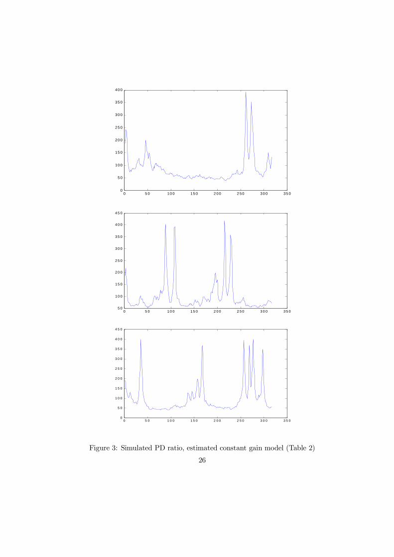
To show that our model also passes an ‘eyeball test’, we report in Figure 3three ‘typical’ realizations of the PD ratio from the estimated baseline modelfor the same number of quarters as shown in Figure 1 for the data. The stockPD ratio in our simulations has the tendency to display sustained priceincreases that are followed by rather sharp price reductions and prolongedperiods of low prices, similar to the behavior of the data shown in Figure23Equations (26) and (27) show that a finite asset price under RE is obtained whenever

δ−1 > βRE . Since risk aversion and growth can bring βRE below 1, this allows for δ > 1.For a discussion, see Kocherlakota (1990).

24

1. The figure illustrates that the oscillations around the RE, suggested bythe phase diagram shown in Figure 2, are very persistent and take the formof rather low-frequency movements with occasional sharp outbreaks andreversals to the top.

We now briefly discuss why our model is also able to generate a sizablerisk premium for stocks. Surprisingly, the model generates an ex-post riskpremium for stocks even when investors are risk neutral (γ = 0). To under-stand this feature, note that the realized gross stock return between period0 and period N can be written as the product of three terms

NYt=1

Pt +Dt

Pt−1=

NYt=1

Dt

Dt−1| z =R1

·µPDN + 1

PD0

¶| z

=R2

·N−1Yt=1

PDt + 1

PDt| z =R3

.

The first term (R1) is independent of the way prices are formed, thus cannotcontribute to explaining the emergence of an equity premium. The secondterm (R2) could potentially generate an equity premium but is on averagebelow one in our simulations, while it is slightly larger than one under RE.The equity premium in the learning model must thus be due the last com-ponent (R3). This term is convex in the PD ratio, so that a model thatgenerates higher volatility of the PD ratio (but the same mean value) willalso give rise to a higher equity premium. Therefore, because our learningmodel generates a considerably more volatile PD ratio, it also gives rise toa larger ex-post risk premium.

In summary, the learning model fits the data very well: all eight momentsfrom Table 1 can be matched by just two free parameters and the simulatedPD series are comparable to those of Figure 1. We find this result remark-able. We employed one of the simplest versions of the asset pricing modeland combined with one of the simplest available learning mechanisms whichadds only one free parameter, namely the gain parameter 1/α. Furthermore,agents’ beliefs are found to be close to RE belief. The strict RE version ofthe model, however, is far from matching any of the facts discussed here.

6.2 Robustness

This section shows that the quantitative performance of the model is robustto a number of deviations from the assumptions about the baseline modeland testing procedure imposed in section 5. We consider one deviation at atime.

25

0 5 0 10 0 15 0 2 00 2 50 30 0 35 00

5 0

10 0

15 0

20 0

25 0

30 0

35 0

40 0

0 5 0 1 0 0 1 5 0 2 0 0 2 5 0 3 0 0 3 5 05 0

1 0 0

1 5 0

2 0 0

2 5 0

3 0 0

3 5 0

4 0 0

4 5 0

0 5 0 1 0 0 1 5 0 2 0 0 2 5 0 3 0 0 3 5 00

5 0

1 0 0

1 5 0

2 0 0

2 5 0

3 0 0

3 5 0

4 0 0

4 5 0

Figure 3: Simulated PD ratio, estimated constant gain model (Table 2)

26

Learning about dividends. For simplicity we assumed that agentsknow the true process for dividends. Also, learning about dividends hasbeen considered previously in other papers. In appendix 8.4 we describea model with learning about prices and dividends. Although the analysisis slightly more involved, the basic properties of the model do not change.Table 3 below shows the results and confirms that the parameter estimatesare largely unchanged and that the model fit remains very good.

Consumption data. Throughout the paper we made the simplifyingassumption Ct/Ct−1 = Dt/Dt−1. We calibrated this process to dividenddata since the variance of dividends has to be brought out when studyingstock price volatility. Since actual consumption growth is much less volatilethan dividend growth, this is a somewhat unsatisfactory aspect. We nowcalibrate the volatility of the consumption and dividend processes separatelyto the data.24 While the dividend process remains as before, we set

Ct+1

Ct= aεct+1 for ln εct ∼ iiN(−s

2c

2; s2c)

The presence of two shocks modifies the equations for the RE version of themodel in a well known way and we do not describe it in detail here. Wecalibrate the consumption process following Campbell and Cochrane (1999),i.e., set sc = s

7 and ρ(εct , εt) = .2.25

The quantitative results are reported in table 3. The match of the risk-free rate now worsens and the corresponding t-ratio falls outside the 95%confidence interval. Equivalently, one could say that the model now mar-ginally fails in matching the risk premium puzzle. Clearly, this occurs be-cause the agents’ stochastic discount factor is now less volatile. For a numberof reasons, we do not wish to over-interpret this deterioration in the modelfit. First, the rejection is marginal, the highest t-ratio is still remains below3. Second, the equity premium is not the main focus of this paper and themodel continues to perform well along the other dimensions of the data.Finally, to a RE fundamentalist, who might dismiss models of learning fromthe outset as being ‘non rigorous because they can always match any data’,this finding illustrates that models of learning can be rejected by the datain the same way as RE models.24For the learning model to be consistent with internal rationality this requires assuming

that the process for income follows a different process than that for dividends, that agentshave rational expectations about this additional process, and that dividend income isagain a minor part of agents’ total income.25We take these ratios and values from table 1 in Campbell and Cochrane (1999), which

is based on a slightly shorter sample than the one used in this paper.

27

Restricting δ ≤ 1 As explained before, the estimated value of thediscount factor is larger than one in the baseline case. Although this does notgenerate any inconsistency in our model or even under RE, some economistsmay feel uncomfortable with discount factors larger than one. Table 3 showsthat the model behaves almost as well when the constraint δ ≤ 1 is imposed.

US Data Learning on Div. Ct/Ct−1 6= Dt/Dt−1 δ ≤ 1Statistic t-ratio t-ratio t-ratio

E(rs) 2.41 2.20 0.48 2.01 0.89 2.26 0.34E(rb) 0.18 0.43 -1.06 0.74 -2.45 0.44 -1.11

E(PD) 113.20 111.58 0.11 111.43 0.12 109.82 0.22σrs 11.65 14.22 -0.89 13.63 -0.69 14.55 -1.00σPD 52.98 74.16 -1.28 73.92 -1.27 74.60 -1.31

ρPD,−1 0.92 0.94 -0.95 0.94 -0.83 0.94 -0.81c25 -0.0048 -0.0054 0.2844 -0.0068 0.9950 -0.0059 0.5344R25 0.1986 0.2133 -0.1777 0.1588 0.4804 0.2443 -0.5516

Parameters:bδ 1.000075 1.010051 11/bα 0.0061 0.0082 0.0063

Table 3: Robustness to model choice

Model-generated standard deviations We now consider deviationsfrom the baseline testing procedure. We first use t-ratios using a model-implied standard deviation of the moments bσSi , closer to standard practicein calibration exercises. For this case δ is chosen to match bE ¡rb¢ exactlysince the model implied standard deviation is bσE(rb) = 0. Clearly, the cor-responding t−ratio is undefined. Table 4 below reports the fit of the model.Although there is some worsening relative to the baseline findings, the over-all fit remains very good.

Full Weighting matrix A classical econometrician might complainthat using a diagonal weighting matrix W as in (33) yields consistent butinefficient estimates of δ, α. We now use an efficient weighting matrix Wderived from standard MSM results. The procedure is described in appendix8.5.2. Table 4 below shows that the fit of the model worsens, some of the

28

t-ratios approach the rejection area, but the overall fit remains surprisinglygood

Overall, the results in this section show that our quantitative resultsare robust to many deviations from the baseline model and baseline testingprocedure.

US Data Model σSi Full matrixStatistic t-ratio t-ratio

E(rs) 2.41 2.25 0.66 1.61 1.77E(rb) 0.18 0.18 – 0.08 0.47

E(PD) 113.20 114.34 -0.06 137.58 -1.61σrs 11.65 15.36 -1.41 10.99 0.23σPD 52.98 76.24 -2.02 67.19 -0.86

ρPD,−1 0.92 0.94 -0.69 0.96 -1.97c25 -0.0048 -0.0062 1.6977 -0.0056 0.4006R25 0.1986 0.2376 -0.7887 0.3646 -2.0047

Parameters:δ 1.002526 1.003587

1/α1 0.0063 0.0045

Table 4: Robustness to testing procedure

7 Conclusions and Outlook

A very simple consumption based asset pricing model is able to quanti-tatively replicate a number of important asset pricing facts, provided oneslightly relaxes the assumption that agents perfectly know how stock pricesare formed in the market. We assume that agents formulate their doubtsabout market outcomes using a consistent set of subjective beliefs aboutprices which is close to, but not equal to, the RE prior beliefs typicallyassumed in the literature. Agents then optimally learn about the equilib-rium price process using past price observations and this gives rise to aself-referential model of learning that imparts momentum and mean rever-sion behavior into the price dividend ratio. As a result, sustained departuresof asset prices from their fundamental value emerge, even though all agentsact rationally in the light of their beliefs.

Given the difficulties documented in the empirical asset pricing literaturein accounting for these facts under RE, our results suggest that modelsof learning may be economically more relevant than previously thought.

29

Indeed, the most convincing case for models of learning can be made byexplaining facts that appear ‘puzzling’ from the RE viewpoint, as we attemptto do in this paper.

The fact that stock prices can deviate for a long time from their funda-mental value in a way that matches the data, even in a model with rationalbehavior, near-RE expectations and no frictions, is likely to have a widerange of practical implications that are worth exploring in future work. Asa result of our findings, asset market and banking regulations could be seenin a rather different light. Accounting rules requiring that institutions markassets to market appear arbitrary, if prices do not reflect the true assetvalue but rather the optimism or pessimism of investors about future capi-tal gains. The effects of shortselling constraints on market outcomes mightequally have to be reassessed: on the one hand such constraints could pre-vent agents from leveraging their (optimistic or pessimistic) expectations,on the other hand they could prevent useful speculation against the pre-vailing market sentiment. Finally, the theory of portfolio choice would haveto be generalized to take into account the state of market expectations inaddition to the state of fundamentals, something that appears familiar topractitioners for quite some time already.

References

Adam, K. (2003): “Learning and Equilibrium Selection in a MonetaryOverlapping Generations Model with Sticky Prices,” Review of EconomicStudies, 70, 887—908.

Adam, K., and A. Marcet (forthcoming): “Internal Rationality, Imper-fect Market Knowledge and Asset Prices,” Journal of Economic Theory.

Adam, K., A. Marcet, and J. P. Nicolini (2008): “Stock MarketVolatility and Learning,” ECB Working Paper No. 862.

Branch, W., and G. W. Evans (forthcoming): “Asset Return Dynamicsand Learning,” Review of Financial Studies, University of Oregon mimeo.

Brennan, M. J., and Y. Xia (2001): “Stock Price Volatility and EquityPremium,” Journal of Monetary Economics, 47, 249—283.

Brock, W. A., and C. H. Hommes (1998): “Heterogeneous Beliefs andRoutes to Chaos in a Simple Asset Pricing Model,” Journal of EconomicDynamics and Control, 22, 1235—1274.

30

Bullard, J., and J. Duffy (2001): “Learning and Excess Volatility,”Macroeconomic Dynamics, 5, 272—302.

Campbell, J. Y. (2003): “Consumption-Based Asset Pricing,” inHandbookof Economics and Finance, ed. by G. M. Constantinides, M. Harris, andR. Stulz, pp. 803—887. Elsevier, Amsterdam.

Campbell, J. Y., and J. H. Cochrane (1999): “By Force of Habit: AConsumption-Based Explanation of Aggregate Stock Market Behavior,”Journal of Political Economy, 107, 205—251.

Carceles-Poveda, E., and C. Giannitsarou (2007): “Asset Pricingwith Adaptive Learning,” Review of Economic Dynamics (forthcoming).

Cecchetti, S., P.-S. Lam, and N. C. Mark (2000): “Asset Pricing withDistorted Beliefs: Are Equity Returns Too Good to Be True?,” AmericanEconomic Review, 90, 787—805.

Cochrane, J. H. (2005): Asset Pricing (Revised Edition). Princeton Uni-versity Press, Princeton, USA.

Cogley, T., and T. J. Sargent (2008): “The Market Price of Risk andthe Equity Premium: A Legacy of the Great Depression?,” Journal ofMonetary Economics, 55, 454—476.

Evans, G. W., and S. Honkapohja (2001): Learning and Expectationsin Macroeconomics. Princeton University Press, Princeton.

Harrison, J. M., and D. M. Kreps (1978): “Speculative Investor Be-havior in a Stock Market with Heterogeneous Expectations,” QuarterlyJournal of Economics, 92, 323—336.

Kocherlakota, N. (1990): “On the ’Discount’ Factor in GrowthEconomies,” Journal of Monetary Economics, 25, 43—47.

LeRoy, S. F., and R. Porter (1981): “The Present-Value Relation: TestBased on Implied Variance Bounds,” Econometrica, 49, 555—574.

Lucas, R. E. (1978): “Asset Prices in an Exchange Economy,” Economet-rica, 46, 1426—1445.

Marcet, A., and T. J. Sargent (1989): “Convergence of Least SquaresLearning Mechanisms in Self Referential Linear Stochastic Models,” Jour-nal of Economic Theory, 48, 337—368.

31

(1992): “The Convergence of Vector Autoregressions to Ratio-nal Expectations Equilibria,” in Macroeconomics: A Survey of ResearchStrategies, ed. by A. Vercelli, and N. Dimitri, pp. 139—164. Oxford Uni-versity Press, Oxford.

Pastor, L., and P. Veronesi (2003): “Stock Valuation and LearningAbout Profitability,” Journal of Finance, 58(5), 1749—1789.

Shiller, R. J. (1981): “Do Stock Prices Move Too Much to Be Justifiedby Subsequent Changes in Dividends?,” American Economic Review, 71,421—436.

(2005): Irrational Exuberance: Second Edition. Princeton Univer-sity Press, Princeton, USA.

Timmermann, A. (1993): “How Learning in Financial Markets GeneratesExcess Volatility and Predictability in Stock Prices,” Quarterly Journalof Economics, 108, 1135—1145.

(1996): “Excess Volatility and Predictability of Stock Prices in Au-toregressive Dividend Models with Learning,” Review of Economic Stud-ies, 63, 523—557.

32

8 Appendix

8.1 Data Sources

Our data is for the United States and has been downloaded from ‘The GlobalFinancial Database’ (http://www.globalfinancialdata.com). The period cov-ered is 1925:4-2005:4. For the subperiod 1925:4-1998:4 our data set corre-sponds very closely to Campbell’s (2003) handbook data set available athttp://kuznets.fas.harvard.edu/~campbell/ data.html.

In the calibration part of the paper we use moments that are based onthe same number of observations. Since we seek to match the return pre-dictability evidence at the five year horizon (c25 and R

25) we can only use data

points up to 2000:4. For consistency the effective sample end for all othermoments reported in table 1 has been shortened by five years to 2000:4. Inaddition, due to the seasonal adjustment procedure for dividends describedbelow and the way we compute the standard errors for the moments de-scribed in appendix 8.5, the effective starting date was 1927:2.

To obtain real values, nominal variables have been deflated using the‘USA BLS Consumer Price Index’ (Global Fin code ‘CPUSAM’). The monthlyprice series has been transformed into a quarterly series by taking the indexvalue of the last month of the considered quarter.

The nominal stock price series is the ‘SP 500 Composite Price Index(w/GFD extension)’ (Global Fin code ‘_SPXD’). The weekly (up to the endof 1927) and daily series has been transformed into quarterly data by takingthe index value of the last week/day of the considered quarter. Moreover,the series has been normalized to 100 in 1925:4.

As nominal interest rate we use the ‘90 Days T-Bills Secondary Market’(Global Fin code ‘ITUSA3SD’). The monthly (up to the end of 1933), weekly(1934-end of 1953), and daily series has been transformed into a quarterly se-ries using the interest rate corresponding to the last month/week/day of theconsidered quarter and is expressed in quarterly rates, i.e., not annualized.

Nominal dividends have been computed as follows

Dt =

µID(t)/ID(t− 1)

IND(t)/IND(t− 1) − 1¶IND(t)

where IND denotes the ‘SP 500 Composite Price Index (w/GFD extension)’described above and ID is the ‘SP 500 Total Return Index (w/GFD exten-sion)’ (Global Fin code ‘_SPXTRD ’). We first computed monthly dividendsand then quarterly dividends by adding up the monthly series. Following

33

Campbell (2003), dividends have been deseasonalized by taking averages ofthe actual dividend payments over the current and preceding three quarters.

8.2 Proof of mean reversion

To prove mean reversion for the general learning scheme of (17) we need thefollowing additional technical assumptions on the updating function ft:

Assumption 1 There is a η > 0 such that ft is differentiable in the interval(−η, η) for all t and, letting

Dt ≡ inf∆∈(−η,η)

∂ft(∆)

∂∆,

we have ∞Xt=0

Dt =∞

This is satisfied by all the updating rules considered in this paper and bymost algorithms used in the stochastic control literature. For example, it isguaranteed in the OLS case where Dt = 1/(t+α1) and in the constant gainwhere Dt = 1/α for all t. If the assumption would fail and

PDt <∞, then

beliefs would get ‘stuck’ away from the fundamental value simply becauseupdating of beliefs ceases to incorporate new information for t large enough.In this case, the growth rate is a certain constant but agents believe it is adifferent constant and agents make systematic mistakes forever. It is unlikelythat such a scheme with

PDt < ∞ would arise as optimal behavior from

any system of beliefs that puts a grain of truth on the actual value of thegrowth rate for stock prices.

Assumption 2 The learning rule satisfies ft(−z) ≥ −z for all z ∈£0, βU

¤and all t.

Since βt ≥ βt−1 + ft (−βt−1) Assumption 2 insures that βt, Pt ≥ 0 forall t, i.e., that agents predict future stock prices to be non-negative. Again,OLS and constant gain learning satisfy this assumption for α1 ≥ 1, as isassumed throughout the paper. Therefore we have 0 ≤ βt ≤ βU for all t.

We start proving mean reversion for the case βt > a. Fix η > 0 smallenough that η < min(η, (βt − a)/2) where η is as in assumption 1.

34

We first prove that there exists a finite t0 ≥ t such that

∆βt ≥ 0 for all et such that t < et < t0, and (35)

∆βt0 < 0 (36)

To prove this, choose ² = η¡1− δβU

¢. It cannot be that ∆βt ≥ ² for allet > t, since > 0 and this would contradict the bound βt ≤ βU . Therefore

∆βt < ² for some finite t ≥ t. Take t ≥ t to be the first period where∆βt < ².

There are two possible cases: either i) ∆βt < 0 or ii) ∆βt ≥ 0.In case i) we have (35) and (36) hold if we take t0 = t.In case ii) βt can not decrease between t and t so that

βt ≥ βt > a+ η

Furthermore, we have

T (βt,∆βt) = a+∆βt1− δβt

< a+²

1− δβt

< a+²

1− δβU= a+ η

where the first equality follows from the definition of T , the first inequalityuses ∆βt < ² and the second inequality that βt < βU and the last equalityfollows from the choice for ². The previous two relations imply

βt > T (βt,∆βt)

This together with (20), εt ≡ 1 and the fact that ft is increasing gives

βt + ft+1 (T(βt,∆βt)− βt) < βt < βt < βU

so that the projection facility does not apply at t+ 1. Therefore

∆βt+1 = ft+1 (T (βt,∆βt)− βt) < 0

and in case ii) we have that (35) and (36) hold for t0 = t+ 1.This shows that (35) and (36) hold for a finite t0. Now we need to show

that from then on beliefs decrease and, eventually, they go below a+ η.Consider η as defined above. First, notice that given any j ≥ 0, if

∆βt0+j

< 0 and (37)

βt0+j

> a+ η (38)

35

then

∆βt0+j+1 = ft0+j+1

µa+

∆βt0+j1− δβt0+j

− βt0+j

¶< ft0+j+1

¡a− βt0+j

¢(39)

< ft0+j+1 (−η) ≤ −ηDt0+j+1 ≤ 0 (40)

where the first inequality follows from (37), the second inequality from (38)and the third from the mean value theorem, η > 0 andDt0+j+1 ≥ 0. Assume,towards a contradiction, that (38) holds for all j ≥ 0. Since (37) holds forj = 0, it follows by induction that ∆βt0+j ≤ 0 for all j ≥ 0 and, therefore,that (40) would hold for all j ≥ 0 hence

βt0+j =

jXi=1

∆βt0+i + βt0 ≤ −ηjX

i=1

Dt0+i + βt0

for all j > 0. Assumption 1 above would then imply βt →−∞ showing that(38) can not hold for all j. Therefore there is a finite j such that βt0+j willgo below a+ η and β is decreasing from t0 until it goes below a+ η.

For the case βt < a − η we need to make the additional assumptionthat βU > a. Then, choosing ² = η we can use a symmetric argument toconstruct the proof.

8.3 Details on the phase diagram

The second order difference equation (20) with εt ≡ 1, which describesthe deterministic evolution of beliefs, allows to construct the directionaldynamics in the

¡βt, βt−1

¢plane shown in Figure 2. Here we show the

algebra leading to the arrows displayed in this figure. For clarity, we definex0t ≡ (x1,t, x2,t) ≡

¡βt, βt−1

¢, whose dynamics are given by

xt+1 =

Ãx1,t + ft+1

³a+

aδ(x1,t−x2,t)1−δx1,t − x1,t

´x1,t

!The points in Figure 2 where there is no change in each of the elements ofx are the following: we have ∆x2 = 0 at points x1 = x2, so that the 45o linegives the point of no change in x2, and ∆x2 > 0 above this line. We have∆x1 = 0 for x2 = 1

δ −x1(1−δx1)

aδ , this is the curve labelled ”βt+1 = βt” inFigure 2 and we have ∆x1 > 0 below this curve. So the zeroes for ∆x1 and∆x2 intersect are at x1 = x2 = a which is the REE and, interestingly, atx1 = x2 = δ−1 which is the limit of rational bubble equilibria. These resultsgive rise to the directional dynamics shown in figure 2.

36

8.4 Model with learning about dividends

This section considers agents who learn to forecast future dividends in addi-tion to forecast future price. We make the arguments directly for the generalmodel with risk aversion from section 5. Equation (25) then becomes

Pt = δEPt

µµDt

Dt+1

¶γ

Pt+1

¶+ δEPt

ÃDγt

Dγ−1t+1

!(41)

Under RE one has

Et

ÃDγt

Dγ−1t+1

!= Et

õDt+1

Dt

¶1−γ!Dt

= Et

³(aε)1−γ

´Dt

= βREDt

Definining the (risk-adjusted) dividend growth forecast as

βDt ≡ EPt

õDt+1

Dt

¶1−γ!agents’ forecast of the latter term in (41) is given by

EPt

ÃDγt

Dγ−1t+1

!= βDt Dt

Under the belief specification described in section 4.3, agents’ conditionalexpectations for dividend growth evolve according to

βDt = βDt−1 +1

αt

õDt−1Dt−2

¶1−γ− βDt−1

!(42)

where the gain sequence 1/αt is the same as the one used for updating theestimate for risk-adjusted stock price growth βt, which continues to evolveaccording to equation (31). As with stock price growth expectations, wecenter initial beliefs for dividend growth at the RE outcome, which implies

βDt = βRE .

With these assumptions, equation (41) implies that the equilibrium price isgiven by

Pt =δβDt1− δβt

Dt

37

Since βDt → a for the decreasing gain case, and since βDt will fluctuate closelyaround a for small but constant gain values, the pricing implications withdividend learning are very similar those derived for the case where agentshave RE about the dividend process.

8.5 Details of the testing procedure

This appendix describes details of our baseline testing approach and givesestimators of the standard deviation of the sample statistics reported intable 2.

8.5.1 Baseline estimation and testing

Here we show that the estimator defined in (33) is consistent and we derivethe asymptotic distribution for the moments of the model we report.

Let N be the sample size, (y1, ...,yN) the observed data sample, with ytcontainingm variables. In the text we talked about "moments" as describingall statistics to be matched in (32) even though some of these statistics arenot proper moments, they are only functions of moments. In this appendixwe properly use the term "statistic" as possibly different from "moment".

We consider sample statistics S(cMN ) where S : Rq → Rs is a statisticfunction that maps sample moments cMN into the considered statistics. Themoments are defined by cMN ≡ 1

N

PNt=1 h(yt) for a given function h : R

m →Rq. The explicit expressions for h(·) and S(·) for our particular applicationare stated in 8.5.3 below.

Since we match these statistics instead of proper moments this is not animmediate application of standard MSM, so we adapt standard proofs toderive the asymptotic theory results that are needed.

In the main text we have denoted the observed sample statistics as bS ≡S(cMN). Let yt(θ) be the series generated by the model for parameter valuesθ and some realization of the underlying shocks, let θ0 be the true parametervalue, M0 ≡ E [ h(yt(θ0)) ] are the true moments, M(θ) ≡ E [ h(yt(θ)) ] arethe true moments for parameter values θ at the stationary distribution foryt(θ) and eS(θ) ≡ S(M(θ)) are the true statistics when the model parameteris θ.

Using standard results from MSM, the estimates bδ, bα defined by (33)converge asymptotically to their true values if the following conditions hold:y is stationary and ergodic, the effect of initial conditions dies down suffi-ciently quickly, W converges almost surely to a positive definite matrix fW

38

as the sample grows, andh eS(θ0)− eS(θ)i0 fW h eS(θ0)− eS(θ)i = 0holds only for θ = θ0, i.e., the set of statistics uniquely identifies θ0. Thelatter identification assumption typically requires the number of parametersto be less than the number of statistics s.

Denote by M j0 the j-th autocovariance of the moment function at the

true parameter, that is

M j0 ≡ E[ [h(yt(θ0))−E(h(yt(θ0))] [h(yt−j(θ0))− E(h(yt−j(θ0))]

0 ]

Define

Sw ≡∞X

j=−∞M j0 (43)

we have the following

Result 1: Suppose that in addition to the assumptions required for consis-tency we have

• Sw <∞,

• a consistent estimator bSw,N such that bSw,N → Sw a.s. asN →∞,and

• S is continuously differentiable at M0.

Then, defining

bΣS,N ≡ ∂S(MN)

∂M 0bSw,N ∂S(MN)

0

∂M

and letting bσSi denote the square root of the i-th diagonal element of1NbΣS,N , we have thatbSi − Si(M0)bσSi → N (0, 1) in distribution as N →∞. (44)

for each i = 1, ..., s whenever the model is true.

Proof. The proof uses standard arguments, we just give an outline. Thecentral limit theorem implies

√NhcMN −M0

i→ N (0, Sw) in distribution

39

The mean value theorem implies√N [S(MN)− S(M0)] → N (0,ΣS) in distribution for (45)

ΣS =∂S(M0)

∂M 0 Sw∂S 0(M0)

∂M(46)

Since cMN →M0 a.s. we have bΣS,N → ΣS a.s. which implies (44).Therefore, the denominator of (34) is found by combining an estimator

of Sw with∂S(MN )∂M 0 to obtain the variance-covariance matrix of the statisticsbΣS,N . Consistent estimates bSw,N can be obtained from the data by using

the Newey West estimator, which substitutes the expectations in (43) bythe sample means, truncates the infinite sum and gives decreasing weightto the sample autocovariances at longer lags. This is standard and we donot describe the details here. An explicit expression for ∂S/∂M 0 for thestatistics (32) that we match is given in appendix 8.5.4. Notice that bΣS,Ncan be formed using data only, the model or its parameter estimates do notenter the computation.

There are various ways to compute the moments of the model eS(θ) fora given θ ∈ Rn.We use the following Monte-Carlo procedure. Let ωi denotea realization of shocks drawn randomly from the known distribution thatthe underlying shocks are assumed to have and

¡y1(θ, ωi), ...yN (θ, ωi)

¢the

random variables corresponding to a history of length N generated by themodel for shock realization ωi and parameter values θ. Furthermore, let

MN(θ, ωi) ≡ 1

N

NXt=1

h(yt(θ, ωi))

denote the model moment for realization ωi. We set the model statisticseS(θ) equal to1

K

KXi=1

S(MN (θ, ωi))

for largeK. In other words, eS(θ) is an average across a large number of simu-lations of lengthN of the statistics S(MN (θ, ωi)) implied by each simulation.We use K of the order of 1000, so any error introduced by the simulation isvery small. These are the averages reported as model moments in tables 2to 4 of the main text.

Our baseline procedure uses a diagonal weighting matrixW where the di-agonal contains the inverse of the diagonal elements of bSw,N . This procedurethus finds parameters that match the model statistics as closely as possible

40

to the data statistics, but gives less weight to statistics with a larger stan-dard deviation. Notice that the calibration result is invariant to a rescalingof the variables of interest.

8.5.2 Full matrix estimation

We chose a diagonal W in the baseline calibration for simplicity. As iswell known an efficient matrix that minimizes asymptotic variance of theestimators given the statistics to be matched amounts to settingW = bΣ−1S,N .The resulting estimates and tests are the ones described in the last columnsof table 4. For bΣS,N to be invertible one requires that s ≤ q. In our case wehave s = 8 and q = 9.

8.5.3 The statistic and moment functions

This section gives explicit expressions for the statistic function S(·) andthe moment functions h(·) that map our estimates into the framework justdiscussed in this appendix.

The underlying sample moments are

MN ≡1

N

NXt=1

h(yt)

where h(·) : R42 → R9 and yt are defined as

h(yt) ≡

⎡⎢⎢⎢⎢⎢⎢⎢⎢⎢⎢⎢⎢⎢⎢⎣

rstPDt

(rst )2

(PDt)2

PDt PDt−1rs,20t−20³rs,20t−20

´2rs,20t−20PDt−20

rbt

⎤⎥⎥⎥⎥⎥⎥⎥⎥⎥⎥⎥⎥⎥⎥⎦, yt ≡

⎡⎢⎢⎢⎢⎢⎢⎢⎢⎢⎢⎢⎢⎢⎣

PDt

Dt/Dt−1PDt−1

Dt−1/Dt−2...

PDt−19Dt−19/Dt−20

PDt−20rbt

⎤⎥⎥⎥⎥⎥⎥⎥⎥⎥⎥⎥⎥⎥⎦where rs,20t denotes the stock return over 20 quarters, which can be computedusing from yt using (PDt,Dt/Dt−1, ..., PDt−19, Dt−19/Dt−20).

41

The eight statistics we consider can be expressed as function of the mo-ments as follows:

S(M) ≡

⎡⎢⎢⎢⎢⎢⎢⎢⎢⎢⎢⎣

E(rst )E(PDt)σrstσPDt

ρPDt,−1c52R25

E(rbt )

⎤⎥⎥⎥⎥⎥⎥⎥⎥⎥⎥⎦=

⎡⎢⎢⎢⎢⎢⎢⎢⎢⎢⎢⎢⎢⎢⎣

M1

M2qM3 − (M1)

2qM4 − (M2)

2

M5−(M2)2

M4−(M2)2

c52(M)R25(M)M9

⎤⎥⎥⎥⎥⎥⎥⎥⎥⎥⎥⎥⎥⎥⎦where Mi denotes the i−th element of M and the functions c52(M) andR25(M) define the OLS and R2 coefficients of the excess returns regressions,more precisely

c5(M) ≡∙1 M2

M2 M4

¸−1 ∙M6

M8

¸R25(M) ≡ 1−

M7 − [M6,M8] c5(M )

M7 − (M6)2

42

8.5.4 Derivatives of the statistic function

This appendix gives explicit expressions for ∂S/∂M 0 using the statistic func-tion stated in appendix 8.5.3. Straightforward but tedious algebra shows

∂Si∂Mj

= 1 for (i, j) = (1, 1), (2, 2), (8, 9)

∂Si∂Mi

=1

2Si(M)for i = 3, 4

∂Si∂Mj

=−Mj

Si(M )for (i, j) = (3, 1), (4, 2)

∂S5∂M2

=2M2(M5 −M4)

(M4 −M22 )2

,∂S5∂M5

=1

M4 −M22

,∂S5∂M4

= − M5 −M22¡

M4 −M22

¢2∂S6∂Mj

=∂c52(M)

∂Mjfor i = 2, 4, 6, 8

∂S7∂Mj

=[M6,M8]

∂c5(M)∂Mj

M7 −M26

for j = 2, 4

∂S7∂M6

=

hc51(M) + [M6,M8]

∂c5(M )∂M6

i ¡M7 −M2

6

¢− 2M6 [M6,M8] c

5(M)¡M7 −M2

6

¢2∂S7∂M7

=M26 − [M6,M8] c

5(M)¡M7 −M2

6

¢2∂S7∂M8

=c52(M) + [M6,M8]

∂c5(M)∂M8

M7 −M 26

Using the formula for the inverse of a 2x2 matrix

c5(M) =1

M4 −M22

∙M4M6 −M2M8

M8 −M2M6

¸

43

we have

∂c5(M)

∂M2=

1

M4 −M22

µ2M2c

5(M)−∙M8

M6

¸¶∂c5(M)

∂M4=

1

M4 −M22

µ−c5(M) +

∙M6

0

¸¶∂c5(M)

∂M6≡ 1

M4 −M22

∙M4

−M2

¸∂c5(M)

∂M8≡ 1

M4 −M22

∙−M2

1

¸All remaining terms ∂Si/∂Mj not listed above are equal to zero.

8.5.5 Differentiable projection facility

As discussed in the main text, we introduce a projection facilitye that pre-vents perceived stock price growth βt from being higher than δ−1, so as toinsure a finite stock price. In addition, it is convenient for our calibration ex-ercises if the learning scheme is a continuous and differentiable function, seethe discussion in appendix 8.5. The standard projection facility describedin (17) causes the simulated equilibrium price series Pt(θ, ωi) for a givenshock realization ωi to be discontinuous as a function of the parameters θ.This is because the price will jump at a parameter value where the facilityis exactly binding.

We thus introduce a projection facility that ‘phases in’ more gradually.We define

β∗t = βt−1 +1

αt

"µDt−1Dt−2

¶−γ Pt−1Pt−2

− βt−1

#(47)

and modify the updating scheme (31) to

βt =

½β∗t if β∗t ≤ βL

βL +w(β∗t − βL)(βU − βL) otherwise(48)

for some weighting function w, and constants βU , βL. Here βU < δ−1 is theupper bound on beliefs, chosen to insure that the implied PD ratio is alwaysless than a certain upper bound UPD ≡ δa

1−δβU , the constant βL < βU is

some arbitrary level of beliefs above which the projection facility starts to

44

operate and w(·) : R+ → [0, 1] is a weighting function. Since w takes valuesbetween zero and one this formula insures that the beliefs are below βU . Wefurther require that w is increasing, w(0) = 0 and w(∞) = 1, and we wantto insure that the resulting beliefs βt are continuously differentiable w.r.t.β∗t at the point β

L.In particular, we use

w(x) = 1− βU − βL

x+ βU − βL.

With this weighting function

limβ∗t%βL

βt = limβ∗t&βL

βt = βL

limβ∗t%βL

∂βt∂β∗t

= limβ∗t&βL

∂βt∂β∗t

= 1

limβ∗t→∞

βt = βU

In our numerical applications we choose βU so that the implied PD rationever exceeds UPD = 500 and βL = δ−1 − 2(δ−1 − βU), which implies thatthe dampening effect of the projection facility starts to come into effect forvalues of the PD ratio above 250.

The figure below shows how the standard projection facility in (17) op-erates versus the continuous projection facility proposed in this appendix.It displays the discontinuity introduced by the standard projection facilityand that for most β∗ the projection facility is irrelevant. For this graphβRE = 1.0035.

The continuous dampening of observations for high stock price growththat is implied by this continuous projection facility is analogous to theone that would arise from optimally incorporating new information given aconsistent beliefs and a prior about βP that is bounded above by βU .

8.6 Convergence of least squares to RE

We show global convergence when agents use least squares learning and theyhave risk aversion as in section 5. The proof shows global convergence, thatis, it obtains a stronger result than is usually found in many applicationsof least squares learning using the associated o.d.e. approach. The proofbelow is for the standard projection facility.

45

Figure 3: Projection Facilities

1,003

1,005

1,007

1,009

1,003 1,005 1,007 1,009 1,011

beta-s tar

beta Standard Proj beta Cont Proj betaL betaU

Figure 4:

46

We remove the assumption of log-normality on the ε’s but assumeDt ≥ 0with probability one, which requires that εt ≥ 0. We also need ε1−γt to bebounded above, formally we assume existence of some positive Uε <∞ suchthat

Prob(ε1−γt < Uε) = 1

This excludes log-normality (except for the case of log utility) but it stillallows for a rather general distribution for εt. Obviously, if γ < 1 this issatisfied if εt is bounded above a.s. by a finite constant, and if γ > 1 this issatisfied if εt is bounded away from zero. We also denote UPD ≡ δβU

1−δβU <∞,

this is the highest PD ratio that can be achieved given that the projectionfacility insures βt < βU .

We first show that the projection facility will almost surely cease to bebinding after some finite time. In a second step, we prove that βt convergesto βRE from that time onwards.

The standard projection facility implies

∆βt =

(α−1t

³(aεt−1)

−γ Pt−1Pt−2− βt−1

´if βt−1 + α−1t

³(aεt−1)

−γ Pt−1Pt−2− βt−1

´< βU

0 otherwise(49)

If the lower equality applies one has α−1t (aεt−1)−γ Pt−1

Pt−2≥ βt−1 ≥ 0 and this

shows the following inequality

βt ≤ βt−1 + α−1t

µ(aεt−1)

−γ Pt−1Pt−2

− βt−1

¶(50)

holds for all t a.s., whether or not the projection facility is binding at t. Wealso have that ¯

βt − βt−1¯≤ α−1t

¯(aεt−1)

−γ Pt−1Pt−2

− βt−1

¯(51)

holds for all t a.s., because if βt < βU this holds with equality and if βt−1+

α−1t

³(aεt−1)

−γ Pt−1Pt−2− βt−1

´≥ βU then

¯βt − βt−1

¯= 0.

Substituting recursively backwards in (50) for past β’s delivers the first

47

line in

βt ≤1

t− 1 + α1

⎛⎝(α1 − 1) β0 +t−1Xj=0

(aεj)−γ Pj

Pj−1

⎞⎠=

t

t− 1 + α1

⎛⎝(α1 − 1) β0t

+1

t

t−1Xj=0

(a εj)1−γ

⎞⎠| z

=T1

+1

t− 1 + α1

⎛⎝t−1Xj=0

δ ∆βj1− δβj

(aεj)1−γ

⎞⎠| z

=T2

(52)

a.s., where the second line follows from

PtPt−1

=

µ1 +

δ ∆βt1− δβt

¶aεt

Clearly, T1 → 1(0 + E((a εj)1−γ)) = βRE as t → ∞ a.s. Also, if we can

establish |T2|→ 0 a.s. this will show that βt will eventually be bounded awayfrom its upper bound or, more formally, that lim supt→∞ βt ≤ βRE < βU .This is achieved by noting that

|T2| ≤1

t− 1 + α1

t−1Xj=0

δ (a εj)1−γ

1− δβj

¯∆βj

¯≤ Uε

t− 1 + α1

t−1Xj=0

a1−γδ¯∆βj

¯1− δβj

≤ Uε

t− 1 + α1

δa1−γ

1− δβU

t−1Xj=0

¯∆βj

¯(53)

a.s., where the first inequality results from the triangle inequality and thefact that both εj and 1

1−δβjare positive, the second inequality follows from

the a.s. bound on εj, and the third inequality from βt ≤ βU . Next, observethat a.s. for all t

(aεt)−γ Pt

Pt−1=1− δβt−11− δβt

(aεt)1−γ <

(aεt)1−γ

1− δβt<

a1−γUε

1− δβU(54)

where the equality follows from

Pt =δβRE

1− δβtDt,

48

the first inequality from βt−1 > 0, and the second inequality from the boundson ε and βt. Applying the triangle inequality in the right side of equation(51), using (54) and βt−1 < βU gives the inequality in

1

t− 1 + α1

t−1Xj=0

¯∆βj

¯≤ 1

t− 1 + α1

t−1Xj=0

α−1j

µa1−γUε

1− δβU+ βU

¶

=

µa1−γUε

1− δβU+ βU

¶1

t− 1 + α1

t−1Xj=0

1

j − 1 + α1(55)

the equality follows from simple algebra. Now, for any ζ > 0

t−1tX

i=0

i−1 = tζ−1tX

i=0

t−ζi−1 ≤ t−1+ζtX

i=0

i−(1+ζ) → 0 as t→∞

where the convergence follows from the well known fact that the over-harmonic series

Pti=0 i

−(1+ζ) is convergent. This and the fact that the largeparenthesis in (55) is finite implies

1

t− 1 + α1

t−1Xj=0

¯∆βj

¯→ 0 for all t a.s.

Then (53) implies that |T2|→ 0 a.s. as t→∞. Taking the lim sup on bothsides of (52), it follows from T1 → βRE and |T2|→ 0 that

lim supt→∞

βt ≤ βRE < βU

a.s. The projection facility is thus binding finitely many periods with prob-ability one.

We now proceed with the second step of the proof. Consider for a givenrealization a finite period t where the projection facility is not binding forall t > t. Then the upper equality in (49) holds for all t > t and simplealgebra gives

βt =1

t− t+ αt

⎛⎝t−1Xj=t

(aεj)−γ Pj

Pj−1+ αt βt

⎞⎠=

t− t

t− t+ αt

⎛⎝ 1

t− t

t−1Xj=t

(aεj)1−γ +

1

t− t

t−1Xj=t

δ ∆βj1− δβj

(aεj)1−γ +

αtt− t

βt

⎞⎠(56)

49

for all t > t. Equations (50) and (51) now hold with equality for all t > t.Similar operations as before then deliver

1

t− t

t−1Xj=t

δ ∆βj1− δβj

(aεj)1−γ → 0

a.s. for t→∞. Finally, taking the limit on both sides of (56) establishes

βt → a1−γE(ε1−γt ) = βRE

a.s. as t→∞.¥

50

CENTRE FOR ECONOMIC PERFORMANCE

Recent Discussion Papers

1076 Zsófia L. Bárány The Minimum Wage and Inequality - The

Effects of Education and Technology

1075 Joanne Lindley

Stephen Machin

Rising Wage Inequality and Postgraduate

Education

1074 Stephen Hansen

Michael McMahon

First Impressions Matter: Signalling as a

Source of Policy Dynamics

1073 Ferdinand Rauch Advertising Expenditure and Consumer

Prices

1072 Alberto Galasso

Mark Schankerman

Carlos J. Serrano

Trading and Enforcing Patent Rights

1071 Daniel Hale

John Coleman

Richard Layard

A Model for the Delivery of Evidence-Based

PSHE (Personal Wellbeing) in Secondary

Schools

1070 David Marsden Individual Voice in Employment

Relationships: A Comparison Under Different

Forms of Workplace Representation

1069 Ross Levine

Alexey Levkov

Yona Rubinstein

Racial Discrimination and Competition

1068 Klaus Adam

Albert Marcet

Internal Rationality, Imperfect Market

Knowledge and Asset Prices

1067 Yanhui Wu A Simple Theory of Managerial Talent, Pay

Contracts and Wage Distribution

1066 Yanhui Wu Managerial Incentives and Compensation in a

Global Market

1065 Nicholas Bloom

Helena Schweiger

John Van Reenen

The Land that Lean Manufacturing Forgot?

Management Practices in Transition

Countries

1064 Klaus Adam

Pei Kuang

Albert Marcet

House Price Booms and the Current Account

1063 Stephen Hansen

Michael McMahon

How Experts Decide: Identifying Preferences

versus Signals from Policy Decisions

1062 Paul Dolan

Daniel Fujiwara

Robert Metcalfe

A Step towards Valuing Utility the Marginal

and Cardinal Way

1061 Marek Jarocinski

Albert Marcet

Autoregressions in Small Samples, Priors

about Observables and Initial Conditions

1060 Christos Genakos

Kai Uwe Kühn

John Van Reenen

Leveraging Monopoly Power by Degrading

Interoperability: Theory and Evidence from

Computer Markets

1059 Klaus Adam

Albert Marcet

Booms and Busts in Asset Prices

1058 Michael W. L. Elsby

Jennifer C. Smith

Jonathan Wadsworth

The Role of Worker Flows in the Dynamics

and Distribution of UK Unemployment

1057 Fabrice Defever Incomplete Contracts and the Impact of

Globalization on Consumer Welfare

1056 Fadi Hassan The Penn-Belassa-Samuelson Effect in

Developing Countries: Price and Income

Revisited

1055 Albert Marcet

Ramon Marimon

Recursive Contracts

1054 Olivier Cadot

Leonardo Iacovone

Denisse Pierola

Ferdinand Rauch

Success and Failure of African Exporters

1053 Björn Eriksson

Tobias Karlsson

Tim Leunig

Maria Stanfors

Gender, Productivity and the Nature of Work

and Pay: Evidence from the Late Nineteenth-

Century Tobacco Industry

1052 Hartmut Lehmann

Jonathan Wadsworth

The Impact of Chernobyl on Health and

Labour Market Performance

1051 Jörn-Steffen Pischke Money and Happiness: Evidence from the

Industry Wage Structure

1050 Tim Leunig

Joachim Voth

Spinning Welfare: the Gains from Process

Innovation in Cotton and Car Production

1049 Francesca Cornaglia

Andrew Leigh

Crime and Mental Wellbeing

1048 Gianluca Benigno

Hande Küçük-Tuger

Portfolio Allocation and International Risk

Sharing

The Centre for Economic Performance Publications Unit

Tel 020 7955 7673 Fax 020 7955 7595

Email info@cep.lse.ac.uk Web site http://cep.lse.ac.uk