Cellular Automata and Agent-Based Models for Earth Systems

Research

   

Outline

• Introduction to Modelling and Simulation• CA

­ theory and application­ examples

• ABM

­ theory and application­ examples

   

General Principles

• Natural systems can often be represented as continua• These can be represented by continuous discrete fields or by equations 

describing rates of change• Mathematically rates of change are expressed by differential 

equations.• Sometimes precise analytical solutions exist but often they must be 

solved numerically.• Advection and diffusion processes describe the rate of change of 

quantities in time and space.• They are best represented by partial differential equations and 

frequently solved numerically using finite differences/ finite elements.

   

Modelling vs. Simulation

• Modelling: the act of abstracting from the real world and specifying it in some formalism

• Simulation: running the model

   

Discrete vs. Continuous

• Time, Space, & Attributes• Discrete as approximation of continuous• Not either/or

   

Modelling Framework

Following Zeigler et al. 2000

     DEVS

DESS

DTSS

ABM

CA

     Discrete Event/Time/Equation Simulation System

   

 Complexity Theory

• Not a theory• Chaos theory – Edward Lorenz• Related to emergence

   

 Emergence

• Complex behaviour emerges from simple interactions

• Inter­scale emergence vs. intra­scale emergence

emergent global structure

   Stolen from : http://necsi.org/projects/mclemens/cs_char.gif

   

Outline

• Introduction • CA

­ theory and application­ examples

• ABM

­ theory and application­ examples

   

Cellular Automata (CA)

• Discrete dynamical systems

• Discrete = space, time, and properties have finite,  countable states

• Complexity is bottom up

   

CA background

• Early research in the 40’s• Popularised by The Game of Life• Now used in modelling physical and human systems, e.g.  

­ soil erosion­ vegetation dynamics­ urbanization/ land use change­ sand piles

(And studied by a bunch of people obsessed with discovering all of the possible patterns that can be created by CA)

   

CA components

• Cellular Space or Lattice• Cell States• Neighbourhood• Transition Rules• Discrete Time

if (some condition holds)     do x

finite set of cell states

   

Spaces• Traditionally Raster• Vector• Graph• Higher dimensional spaces?

   

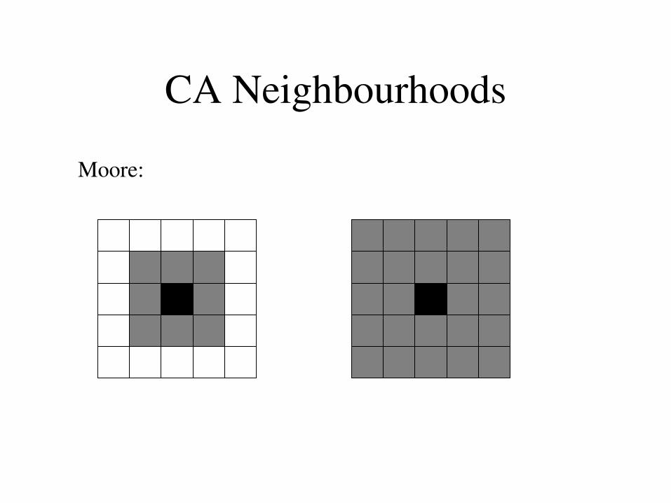
CA Neighbourhoods

Moore:

   

CA Neighbourhoods

von Neumann:

   

CA Neighbourhoods

Arbitrary:

   game of life glider

   

Game of Life Rules

1. A dead cell with exactly 3 live neighbours becomes alive

2. A live cell with 2 or 3 live neighbours stays alive; otherwise it dies. 

t = 4?

   

   Rinaldi E (1999)."The Multi­Cellular Automaton: a tool to build more sophisticated models. A theoretical foundation and a practical implementation" in Rizzi P. e Savino M. (eds) On the edge of the Millennium. Proceedings of Computer in Urban Planning and Urban Management 6th International Conference F. Angeli 1999 (in pubblicazione) e in Proceedings ESIT Creta (in pubblicazione)

   

CA Applications: urban growth

http://www.geog.umd.edu/resac/urban­modeling.htm

Model of Future Growth in the Washington, DC­Baltimore Region 1986­2030 using the SLEUTH model

   

SLEUTH growth coefficients

• dispersion coefficient­ spontaneous or road influenced growth

• breed coefficient­ new spreading centre or road influenced growth

• spread coefficient­ edge growth from spreading centre

• slope coefficient­ lower slopes are easier to build on

• road gravity coefficient­ distance from road influences growth

   

CA results

http://www.geog.umd.edu/resac/urban­modeling­animation1.htm

sloperoads

excluded areas

   

CA Applications: Soil Erosion

• RillGrow 2 by Favis­Mortlock

http://www.soilerosion.net/rillgrow/

   

CELLULAR AUTOMATA IN INTEGRATED MODELLING

Change in cropland area (for food production) by 2080 compared to baseline (%) for the 4 SRES storylines and HADCM3

After: Schröter et al. (2005). Ecosystem service supply and vulnerability to global change in Europe. Science, 310 (5752), 1333­1337

   

Analysis of CA Output

• Plot cell attributes

• Plot number of cells in certain state

• Use metrics for describing spatial pattern

time

no.

Height

Mass

Land Use….etc

e.g. patch size metrics

   

Outline

• Introduction • CA

­ theory and application­ examples

• ABM

­ theory and application­ examples

   

Agent Based Model (ABM)

A representation of a system in which agents interact with each other and their environment using a set of rules 

• Also called multi­agent systems (MAS)

   

if (some condition holds)     do x

ABM Components

• Space (environment)• Agent(s) – rules defining interaction and neighbourhoods

• Discrete Time

   

what is an agent?

Represents:

• some discrete thing in the world (usually a living thing)• something with behaviour

Representation:

• Physically ­ Geometric object• Programmed – an object with attributes and behaviour

   

agent

• behaviour:­ Rational – deterministic / Stochastic­ e.g. BDI algorithm

• communication:­ Stigmergic­ Message passing

   

deterministic agents

+same initial conditions

=same final state

+stochasticity

   

Environmental Examples

?

   

Types of ABM

• Fixed behaviour model vs. evolutionary model­ e.g. genetic algorithms

• Top down vs. or plus bottom up

   

Example – urban land use in East Anglia

• Endogenising the planning process

felled forest

inland bare ground

continuous urban

suburban/rural development

ruderal weed

tilled land

coniferous woodland

deciduous woodland

scrub/orchard

dense shrub moor

bracken

rough/marsh grass

meadow/verge/semi­natural

mown/grazed turf

grass heath

saltmarch

beach and costal bare

inland water

sea/estuary

unclassified

0 6030 km

Source: Lilibeth Acosta­Michlik and Corentin Fontaine; funded by the Tyndall Centre

   

interactions

patches

agents

actions feedbackfeedback

   

Agent­environment interaction and   are β γ

parameters affecting preferences for landscape and service amenities, respectively

After: Caruso, G., Peeters, D. and Cavailhès, J. and Rounsevell, M.D.A. (2007). ‘Spatial configurations and cellular dynamics in a periurban city’. Regional Science and Urban Economics, 00, 000­000 (in press)

   

agentsprivate sectorpublic sector

localplanners

national policyregional

development

non-residential residential

propertydevelopers

individuallandlords

tourismactvities

commercialcorporations

industryinvestors

tourists

non-residential

publicservices industrial

buildings

commercialcentres

individualretailers

hotels

sites ofvisit

…

residential

appartments

individualhouses

patches

feedback feedback

   

1 2 3 4 5 6 7 8 9 10 11 12isolated student HA1 ++ + +++

single person HA2 + +++ ++ ++ +couple HA3 ++ + + +++ ++ +++ ++

couple with dep. children HA4 + ++ +++ + +single­parent family HA5 +++ ++ ++ +

couple with non­dep. children HA6 +++ ++ + +all retired HA7 + + +++ ++ +

CLUSTERS

Residential agents

• Socio­economic data analysis• Agent profiles (household types) & location trends

   

Legend

LSOA_EA_clust12_4fact<all other values>

clust_ward_12.CLUSTER<Null>

1 = HA6 ­ ... ­ HA7

2 = ... ­ HA3/6 ­ HA7

3 = ... ­ ... ­ HA3/4/6

4 = HA7 ­ ... ­ HA3/6

5 = HA5 ­ HA4 ­ ...

6 = ... ­ HA5/7 ­ ...

7 = HA3/4 HA2 ­ ...

8 = HA2 ­ HA3 ­ ...

9 = ... ­ HA2/5 ­ HA4

10 = HA3 ­ HA1/2 ­ HA4

11 = ... ­ HA3 ­ HA1/2

12 = HA1 ­ ... ­ HA5/7

Household agent location preferences

Demographics and coastal zone pressures

   

Residential model runs

R.I.P.

1

14%

cities

2

20%

suburbs

3

39%

periurban& rural

4

25%

coast

stage

% of pop

concentra

te

mainly in

Structu

re

Model run animation

   

Planning agent interactions

   

Infrastructureprovision

Built environment(Type 2: „implementors“

Top­down (Type 1: „policy developers“)

Bottom­up: (Type 3 „lobbyists“)

Environmentalorganisations

Propertydevelopers

Cultural/naturalheritage

Communityforums

Governmentalorganisations

Conceptual planning model

   

ABM as Computational Laboratory

• Testing hypotheses• Testing methodologies• Is your ABM deterministic or has it got a 

stochastic component?• How many simulations is enough?• How do we interpret model results?• Statistical analysis of results

   

Analysis of ABM Output

• Plot agent attributes• Plot number of agents of certain type• Spatial pattern metrics

­ temporal considerations (at a time or over time)

   

Difference between CA and ABM

?

   

What is the goal of modelling?

• to predict the represented system?

• to understand and explain the represented system?

   

ReferencesGeneral Modelling:

• Zeigler, B. P., H. Praehofer, and T. G. Kim, 2000. Theory of Modeling and Simulation: integrating discrete event and continuous complex dynamic systems. Academic Press, San Diego.

CA:

• Torrens, P. M. 2006. Simulating Sprawl. Annals of the Association of American Geographers 96 (2):248­275.

• Coulthard, T. J., M. J. Kirkby, and M. G. Macklin, 2000. Modelling Geomorphic Response to Environmental Change in an Upland Catchment. Hydrological Processes, 14: 2031­2045.

• Favis­Mortlock, D. T., J. Boardman, A. J. Parsons, et al., 2000. Emergence and Erosion: a model for rill initiation and development. Hydrological Processes, 14: 2173­2205.

• Fonstad, M. A. (2006). Cellular automata as analysis and synthesis engines at the geomorphology­ecology interface. Geomorphology, 77, 217­234.

• Langton, C., 1986. Studying Artificial Life with Cellular Automata. Physica D, 22.

• Shiyuan, H. and L. Deren, 2004: Vector Cellular Automata Based Geographical Entity. Proceedings of the 12th International Conference on Geoinformatics ­ Geospatial Information Research: Bridging the Pacific and Atlantic.  University of Gavle, Sweden, 7­9 June.

   

References

ABM:

• Benenson, I. and P. M. Torrens, 2004. Geosimulation: Agent­based Modeling of Urban Phenomena. John Wiley and Sons, Ltd, London.

• Brown, D. G., S. E. Page, R. L. Riolo, et al., forthcoming. Agent­based and Analytical Modeling to Evaluate the Effectiveness of Greenbelts. Environmental Modelling & Software.

• Brown, Daniel G., Riolo, Rick, Robinson, Derek T., North, M., and William Rand (2005) "Spatial Process and Data Models: Toward Integration of Agent­Based Models and GIS" Journal of Geographical Systems, Special Issue on Space­Time Information Systems 7(1): 25­47

• Gimblett, H. R., Ed., 2002: Integrating Geographic Information Systems and Agent­Based Modeling Techniques for Simulating Social and Ecological Processes. Sante Fe Institute Studies in the Sciences of Complexity, Oxford University Press.

• Parker, D.C., Manson, S.M, Janssen, M.A., Hoffmann, M.J., and Deadman, P. 2003 Multi­agent systems for the simulation of land­use and land­cover change: a review Annals of the Association of American Geographers, 93(2). 314­337.

• Papers on the RePast site: repast.sourceforge.net/papers