cdr sample data model

UDC 004.622, DOI: 10.2298/csis0902087C

A Call Detail Records Data Mart: Data Modelling and OLAP Analysis

Dragana Ćamilović 1, Dragana Bečejski-Vujaklija 2 and Nataša Gospić 3,

1 Faculty of Entrepreneurial Management Modene 5, 21000 Novi Sad, Serbia

[email protected] 2 Faculty of Organizational Sciences, University of Belgrade

Jove Ilica 154, 11000 Belgrade, Serbia [email protected]

3 Faculty of Transport and Traffic Engineering, University of Belgrade Vojvode Stepe 305, 11000 Belgrade, Serbia

[email protected]

Abstract. In order to succeed in the market, telecommunications companies are not competing solely on price. They have to expand their services based on their knowledge of customers’ needs gained through the use of call detail records (CDR) and customer demographics. All the data should be stored together in the CDR data mart. The paper covers the topic of its design and development in detail and especially focuses on the conceptual/logical/physical trilogy. Some other design problems are also discussed. An important area is the problem involving time. This is why the implication of time in data warehousing is carefully considered. The CDR data mart provides the platform for Online Analytical Processing (OLAP) analysis. As it is presented in this paper, an OLAP system can help the telecommunications company to get better insight into its customers’ behaviour and improve its marketing campaigns and pricing strategies.

Keywords: Data Warehousing, Data Modelling, Call Detail Records, OLAP.

1. Introduction

After years of being a monopoly market, the telecommunications’ market is now highly competitive. A monopoly does not change much, but competitive markets change a lot. Customers are able to switch providers easily, because there are many of them available. In order to understand their customers and create a better environment for managing customer relationships, many telecommunications companies use call detail analysis to achieve competitive advantage. By understanding customers’ characteristics and behaviour, it is possible to successfully tailor services that meet customers’ needs. This is known as the personalisation, and this concept is not restricted to the

Dragana Ćamilović, Dragana Bečejski-Vujaklija and Nataša Gospić

ComSIS Vol. 6, No. 2, December 2009 88

telecommunications industry. User profiling can be valuable to semantic web (for more information, see [5]), it is successfully applied in banking, financial services and many other industries.

The telecommunications industry has advantage over other sectors because it has a voluminous amount of customer data. Telecommunications companies collect various demographic data (such as name, address, age and gender information) and store call detail records. Call detail records usually include information about originating and terminating phone numbers, the date and time of the call and its duration [13].

Demographic and call detail data can be stored together in a data mart (known as the CDR data mart), and transformed into information that can be analyzed using OLAP tools. This paper covers the data modelling topic in detail. The conceptual, logical and physical data models are introduced as a necessary part of the CDR data mart design and development.

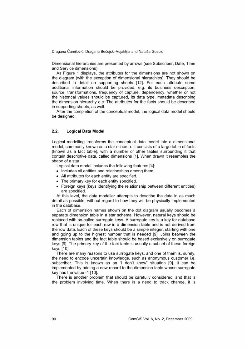
2. Data Modelling: the Conceptual, Logical and Physical Data Models

In the old days there was tradition in which a tree-stage process for designing a database was used [12]. The first model that was developed was the conceptual data model, geared toward the business as a way to describe data requirements at a high level. It was usually presented by an entity relationship (ER) model and it was independent from any particular type of database.

The next step in data modelling was designing the logical data model, which described the precise schema used by the database. Finally, there was the physical data model, consisted of the data definition language (DDL) statements that, in a relational environment, were used to build the tables, indexes and constraints [12].

Today, many relational database designers treat the conceptual, logical and physical model as a same thing – they just build an ER model and convert it directly into a set of tables in the database. However, data warehousing is different, and the conceptual/logical/physical trilogy should absolutely be used.

2.1. Conceptual Data Model

At this level, the data modeller attempts to identify the highest-level relationships among the different entities. As mentioned before, in relational environment the conceptual data model is usually presented by an ER diagram. The ER modelling seeks to remove all redundancy in the data and this is very beneficial to transaction processing. However, ER models are not very suitable for data modelling in data warehousing. In [6], Kimball describes the following reasons for this:



• End users have trouble understanding an ER model. • Software cannot usefully query a general ER model. • ER modelling defeats the basic appeal of data warehousing, and this is

the intuitive and high-performance data retrieval. Of all the reasons, the first one is probably the most important, because

end users play a significant role in defining the business requirements and therefore take an active part in conceptual modelling. This is why the dot modelling technique should be considered. Dot modelling has been well accepted by nontechnical people, and, on the other hand, it provides a structured way for developing a logical model.

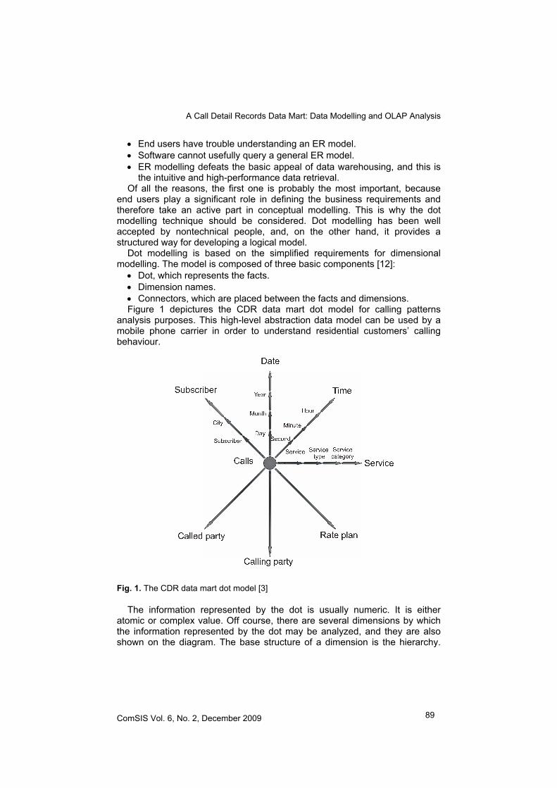
Dot modelling is based on the simplified requirements for dimensional modelling. The model is composed of three basic components [12]:

• Dot, which represents the facts. • Dimension names. • Connectors, which are placed between the facts and dimensions. Figure 1 depictures the CDR data mart dot model for calling patterns

analysis purposes. This high-level abstraction data model can be used by a mobile phone carrier in order to understand residential customers’ calling behaviour.

Fig. 1. The CDR data mart dot model [3]

The information represented by the dot is usually numeric. It is either atomic or complex value. Off course, there are several dimensions by which the information represented by the dot may be analyzed, and they are also shown on the diagram. The base structure of a dimension is the hierarchy.



Dimensional hierarchies are presented by arrows (see Subscriber, Date, Time and Service dimensions).

As Figure 1 displays, the attributes for the dimensions are not shown on the diagram (with the exception of dimensional hierarchies). They should be described in detail on supporting sheets [12]. For each attribute some additional information should be provided, e.g. its business description, source, transformations, frequency of capture, dependency, whether or not the historical values should be captured, its data type, metadata describing the dimension hierarchy etc. The attributes for the facts should be described in supporting sheets, as well.

After the completion of the conceptual model, the logical data model should be designed.

2.2. Logical Data Model

Logical modelling transforms the conceptual data model into a dimensional model, commonly known as a star schema. It consists of a large table of facts (known as a fact table), with a number of other tables surrounding it that contain descriptive data, called dimensions [1]. When drawn it resembles the shape of a star.

Logical data model includes the following features [4]: • Includes all entities and relationships among them. • All attributes for each entity are specified. • The primary key for each entity specified. • Foreign keys (keys identifying the relationship between different entities)

are specified. At this level, the data modeller attempts to describe the data in as much

detail as possible, without regard to how they will be physically implemented in the database.

Each of dimension names shown on the dot diagram usually becomes a separate dimension table in a star schema. However, natural keys should be replaced with so-called surrogate keys. A surrogate key is a key for database row that is unique for each row in a dimension table and is not derived from the row data. Each of these keys should be a simple integer, starting with one and going up to the highest number that is needed [9]. Joins between the dimension tables and the fact table should be based exclusively on surrogate keys [9]. The primary key of the fact table is usually a subset of these foreign keys [10].

There are many reasons to use surrogate keys, and one of them is, surely, the need to encode uncertain knowledge, such as anonymous customer i.e. subscriber. This is known as an “I don’t know” situation [9]. It can be implemented by adding a new record to the dimension table whose surrogate key has the value -1 [10].

There is another problem that should be carefully considered, and that is the problem involving time. When there is a need to track change, it is



unacceptable to make every dimension time-depended to deal with these changes [8]. The independent dimensional structure can be preserved with only relatively minor adjustments to content with changes, and these nearly constant dimensions are referred as slowly changing dimensions (SCDs). For each attribute in a dimension table a strategy to handle change should be specified, and there are three basic techniques than can be used, known as the type 1, type 2 and type 3 responses [8]. With the type 1 response the old attribute value in a dimension row is simply overwritten with the current value. It is easy to implement, but this approach does not maintain any history of prior attribute values. This is why it is appropriate to use it mostly for the purpose of correcting values, and in case there is really no need to capture change.

The type 2 response is the most commonly used when it comes to SCDs. This method attempts to solve the problem of capturing changes by the creation of new records. Every time an attribute's value changes, if faithful recording of history is required, an entirely new record is created with all the unaffected attributes unchanged. Only the affected attribute is changed to reflect its new value. Naturally, a new surrogate key is assigned to the record.

The third type of change solution (type 3) involves recording the current value of an attribute, as well as the original value. In this case an additional column has to be created to contain the extra value. This approach is rarely used.

In practice, the type 1 and type 2 solutions are often combined in the same logical row, if there is a need to track some attributes and some not. In case of the subscriber dimension attributes like the address and, consequently, the city should be tracked, but it is not interesting too keep track of the subscriber’s name. Therefore, in a single logical row, an attribute like address would need to be treated as a type 2, whereas the name would be treated as a type 1.

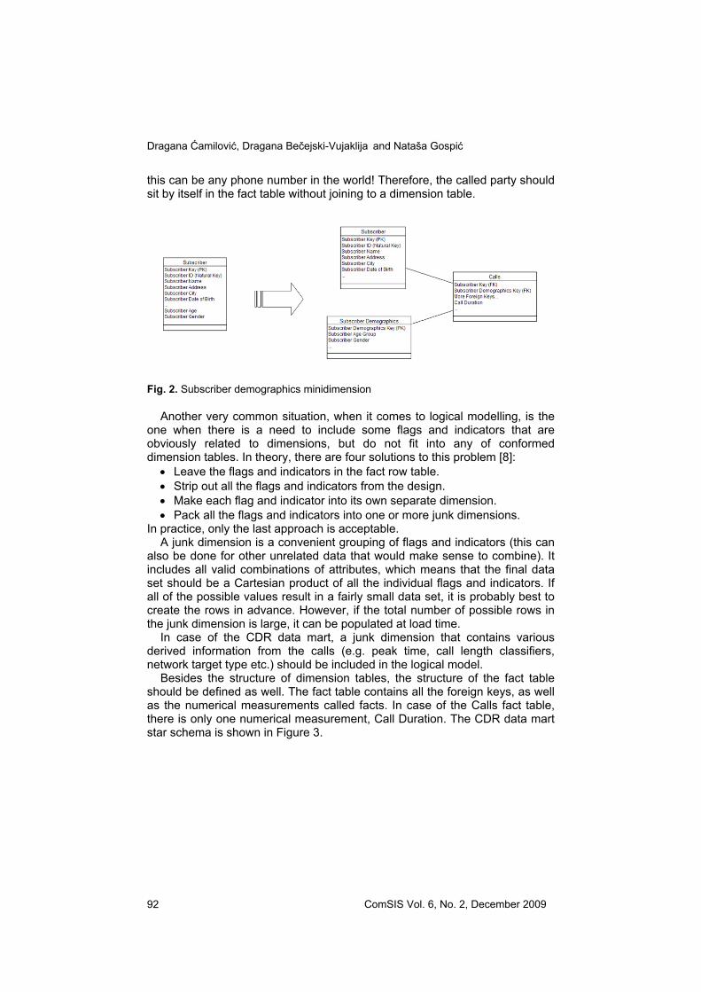
The three solutions presented in this section refer to SCDs. In case of frequently changing attributes it is not appropriate to use any of these approaches. The solution is to break off those frequently changing and frequently analyzed attributes into a separate dimension table, known as minidimension [8]. There would be one row in the minidimension for each unique combination of these attributes. When creating minidimension continuously variable attributes, like age, should be converted to band ranges (in this particular case the age groups should be formed). The subscriber dimension displayed in Figure 1 should be broke into two dimension tables in the star schema: the subscriber dimension table and the subscriber demographics dimension table, as shown in Figure 2.

As mentioned before, each of dimension names shown on the dot diagram usually becomes a separate dimension table in a star schema. However, there is an exception to this rule. Instead of creating the monster dimension, in special cases, it is more appropriate to carry the information in the fact table. Those dimensions are known as degenerate dimensions. The called party in Figure 1 is a perfect candidate for a degenerate dimension, because



this can be any phone number in the world! Therefore, the called party should sit by itself in the fact table without joining to a dimension table.

Fig. 2. Subscriber demographics minidimension

Another very common situation, when it comes to logical modelling, is the one when there is a need to include some flags and indicators that are obviously related to dimensions, but do not fit into any of conformed dimension tables. In theory, there are four solutions to this problem [8]:

• Leave the flags and indicators in the fact row table. • Strip out all the flags and indicators from the design. • Make each flag and indicator into its own separate dimension. • Pack all the flags and indicators into one or more junk dimensions.

In practice, only the last approach is acceptable. A junk dimension is a convenient grouping of flags and indicators (this can

also be done for other unrelated data that would make sense to combine). It includes all valid combinations of attributes, which means that the final data set should be a Cartesian product of all the individual flags and indicators. If all of the possible values result in a fairly small data set, it is probably best to create the rows in advance. However, if the total number of possible rows in the junk dimension is large, it can be populated at load time.

In case of the CDR data mart, a junk dimension that contains various derived information from the calls (e.g. peak time, call length classifiers, network target type etc.) should be included in the logical model.

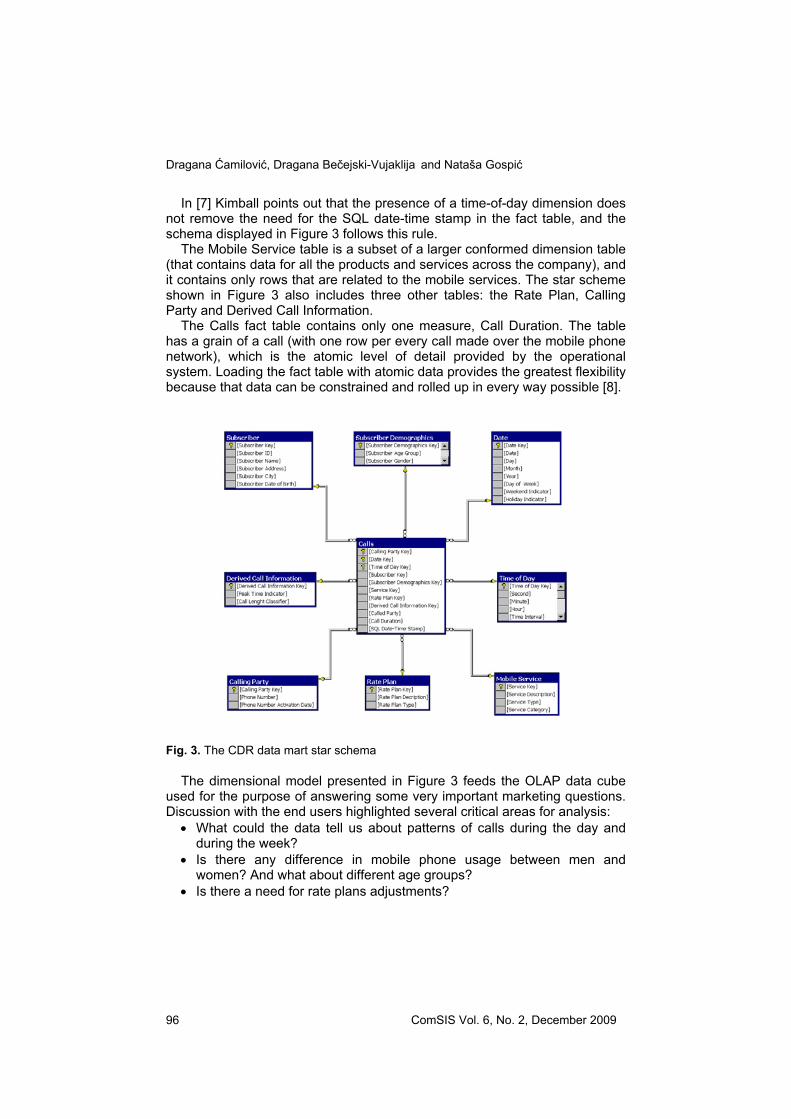
Besides the structure of dimension tables, the structure of the fact table should be defined as well. The fact table contains all the foreign keys, as well as the numerical measurements called facts. In case of the Calls fact table, there is only one numerical measurement, Call Duration. The CDR data mart star schema is shown in Figure 3.



2.3. Physical Data Model

At this level, the data modeller specifies how the logical data model will be realized in the database schema. The objectives of the physical design process do not centre on the structure. The modeller is more concerned about how the model is going to work than on how it is going to look [11].

According to Ponniah, there are several steps in the physical design process for a data warehouse [11]:

• Developing standards. The standards range from how to name the fields in the database to how to conduct interviews with end users for requirements definition. The standard for naming the objects takes on special significance, because the usage of the object names is not confined to the IT specialists. The users also refer to the objects by names, when they create and run their own queries. This is why the name itself must be able to convey the meaning and description of the object. It is also necessary to adopt effective standards for naming the data structures in the staging area, as well as all types of files (not only data and index files, but also files holding source codes and scripts, database files and application documents).

• Creating aggregates plan. In this step, the possibilities for building aggregate tables should be reviewed. It is possible that many of the aggregates will be presented in the OLAP system. However, if OLAP instances are not for universal use by all users, then the necessary aggregates must be presented in the data warehouse. There are two primary factors that should be considered when making a decision about the aggregates plan [8]. First, the business users’ access patterns have to be taken into account – data that they are frequently summarizing on the fly should probably be presented in the data warehouse. Second, the statistical distribution of the data should be assessed (e.g. how many unique instances exist at each level of the hierarchy, and what’s the compression in case of moving from one level to the next) [8].

• Determine the data partitioning schema. Partitioning options for fact tables, as well as dimension tables, should be considered. The data warehouse usually holds some very large database tables. The fact tables run into millions of rows, and many dimension tables (e.g. customer tables) contain a huge number of rows, as well. Having tables of such extremely large sizes faces certain problems. Loading of large tables and building indexes takes excessive time. Queries also run longer, backing up and recovery of huge tables, too. This is why the partitioning is important. Partitioning means deliberate splitting of a table and its index data into manageable parts. The database management system (DBMS) supports and provides the mechanism for this. Each partition of a table is treated as a separate object. The partitions can be spread across multiple disks to gain optimum performance. A large table can be divided vertically or horizontally. In vertical partitioning, one separates out the partitions by grouping selected columns together. In



this scenario, each partitioned table contains the same number of rows as the original table. Usually, wide dimension tables are candidates for vertical partitioning. In case of horizontal partitioning, one divides the table by grouping selected rows together. Horizontal partitioning of the large fact tables based on calendar dates usually works well in a data warehouse environment. The partitioning schema should include the following: the fact tables and the dimension tables selected for partitioning, the type of partitioning for each table (horizontal or vertical), the number of partitions for each table, the criteria for dividing each table and description of how to make queries aware of partitions (a query needs to access only the necessary partitions). Every DBMS has its own specific way of implementing physical partitioning. One of the very important considerations when selecting the DBMS is its support for partitioning and indexing.

• Establishing clustering options. Clustering involves placing and managing related units of data in the same physical block of storage. In this way, those units are retrieved together in a single input operation. In order to establish the proper clustering options, the tables should be carefully examined and pairs that are related should be found. Rows from the related tables are usually accessed together for processing, and it is wise to store them close together in the same file on the medium.

• Preparing an indexing strategy. The indexing plan must indicate the indexes for each table. Further, for each table, the sequence in which the indexes will be created should be defined. Also, the indexes that are expected to be built in the very first instance of the database should be described. The DBMS vendors offer a variety of indexing techniques. The choice is no longer confined to sequential index files. All vendors support B-Tree indexes for efficient data retrieval, as well. Another option is the bit-mapped index. Dimension tables should have a unique index on the single-column primary key. Kimball also recommends a B-tree index on high-cardinality attribute columns used for constraints and placing bit-mapped indexes on all medium- and low-cardinality attributes [8]. In case of fact tables, the primary key is almost always a subset of the foreign keys. In this case it is wise to place a single, concatenated index on the primary dimensions of the fact table. Having the date key also helps in improving performance. Since more than one index can be used in the same time in resolving a query, separate indexes on independent foreign keys in the fact table can be built as well [8] (for more detail on the subject, see [8] and [11]). Indexing is perhaps the most effective mechanism for improving performance. However, having a large number of indexes slows down the loading of data into the warehouse, especially during initial loads. This problem can be solved by dropping the indexes before running the load jobs. In this case, they will not create the index entries during the load process, but constructing the index files can be done after the loading process completes. There is one other thing that should be kept in mind, and that is the fact that large



tables (with millions of rows) cannot support many indexes. When a table is too large, having more than just one index itself could cause difficulties. If more than the one index is necessary, the table should be split before defining more indexes. The most suitable columns for indexing are those that are frequently used to constrain the queries. However, the best practice is to start with indexes on just the primary and foreign keys of each table. Then, after monitoring the performance carefully, some more indexes can be added.

• Assigning storage structures. The storage plan should specify where the data should be placed on the physical storage medium, the physical files, as well as the plan for assigning each table to specific files, and how each physical file should be divided into blocks of data.

• Completing the physical model. This is the final step that reviews and confirms the completion of the prior activities and tasks.

The conceptual/logical/physical trilogy described in this section, in the authors' opinion, is the best practice for data warehouse modelling.

The data warehouse provides the platform for OLAP analysis. Therefore, OLAP is a natural extension of the data warehouse. Armed with an OLAP system, the telecommunications company can get a significant insight into customers. Extracting patterns from customer and usage data and their visual representation is a great help for understanding customer behaviour.

The next section demonstrates the insight gain from data exploration of call detail and post-paid residential subscriber demographic data maintained by a mobile phone carrier that declined to be identified. The project is altered so that no company is recognizable.

3. A Case Study

Call detail record is an important marketing data that mobile phone service provider can analyze to improve customer relationships. These records can be used in conjunction with post-paid residential subscriber demographic data in order to get better and more valuable results. All the data can be put together and stored in an OLAP cube. In this particular case, call detail data is aggregated for three-month period.

The CDR data mart dot model, discussed in the previous section, is the foundation of the star schema shown in Figure 3.

The subscriber dimension is broke into two separate tables (the Subscriber table and the Subscriber Demographics table), as discussed in section 2.2. Time of the day should be separated from the date dimension, to avoid an explosion in the date dimension row count [8] (the dot model displayed in Figure 1 also treats time and date as two separate dimensions). Therefore, it should be a time-of-day dimension table (with one row per second) in the star schema. However, there is always an option to embed a full SQL date-time stamp directly in the fact table for all queries requiring the precision below the level of calendar day [7].



In [7] Kimball points out that the presence of a time-of-day dimension does not remove the need for the SQL date-time stamp in the fact table, and the schema displayed in Figure 3 follows this rule.

The Mobile Service table is a subset of a larger conformed dimension table (that contains data for all the products and services across the company), and it contains only rows that are related to the mobile services. The star scheme shown in Figure 3 also includes three other tables: the Rate Plan, Calling Party and Derived Call Information.

The Calls fact table contains only one measure, Call Duration. The table has a grain of a call (with one row per every call made over the mobile phone network), which is the atomic level of detail provided by the operational system. Loading the fact table with atomic data provides the greatest flexibility because that data can be constrained and rolled up in every way possible [8].

Fig. 3. The CDR data mart star schema

The dimensional model presented in Figure 3 feeds the OLAP data cube used for the purpose of answering some very important marketing questions. Discussion with the end users highlighted several critical areas for analysis:

• What could the data tell us about patterns of calls during the day and during the week?

• Is there any difference in mobile phone usage between men and women? And what about different age groups?

• Is there a need for rate plans adjustments?



The OLAP cube has to include all necessary dimensions and measures. Measures are numeric data needed for analysis purposes, e.g. the total number of calls, the cumulative duration of calls etc. Some measures are more interesting when combined and these are called calculated measures (or calculated members). E.g. the average call duration is interesting for the purpose of calling patterns recognition. It is calculated by dividing the cumulative duration of calls by the total number of calls (made during the three-month period).

The data cube allows data to be viewed in multiple dimensions, e.g. subscriber gender, subscriber age group, day of the week, hour of the day, rate plan etc. The results from OLAP analysis can be presented visually, which enables improved comprehension. As the rest of the section illustrates, the visualization can help answer the questions asked.

3.1. Calls by Day of the Week and by Hour of the Day

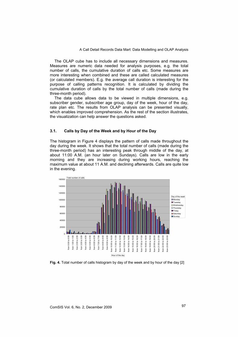
The histogram in Figure 4 displays the pattern of calls made throughout the day during the week. It shows that the total number of calls (made during the three-month period) has an interesting peak through middle of the day, at about 11:00 A.M. (an hour later on Sundays). Calls are low in the early morning and they are increasing during working hours, reaching the maximum value at about 11 A.M. and declining afterwards. Calls are quite low in the evening.

0

20000

40000

60000

80000

100000

120000

140000

160000

from

0:0

0 to

0:5

9

from

1:0

0 to

1:5

9

from

2:0

0 to

2:5

9

from

3:0

0 to

3:5

9

from

4:0

0 to

4:5

9

from

5:0

0 to

5:5

9

from

6:0

0 to

6:5

9

from

7:0

0 to

7:5

9

from

8:0

0 to

8:5

9

from

9:0

0 to

9:5

9

from

10:

00 to

10:

59

from

11:

00 to

11:

59

from

12:

00 to

12:

59

from

13:

00 to

13:

59

from

14:

00 to

14:

59

from

15:

00 to

15:

59

from

16:

00 to

16:

59

from

17:

00 to

17:

59

from

18:

00 to

18:

59

from

19:

00 to

19:

59

from

20:

00 to

20:

59

from

21:

00 to

21:

59

from

22:

00 to

22:

59

from

23:

00 to

23:

59

MondayTuesdayWednesdayThursdayFridaySaturdaySunday

Total number of calls

Hour of the day

Day of the week

Fig. 4. Total number of calls histogram by day of the week and by hour of the day [2]



Figure 4 also shows that the total number of calls has two peaks on Sundays - at midday and at about 5:00 P.M. The total number of calls is lower on weekends. It seems that the calling pattern is quite the same throughout the week (a peak is almost at the same time all week long). An interesting thing to be noticed is that people like to make telephone calls on Wednesdays and Fridays.

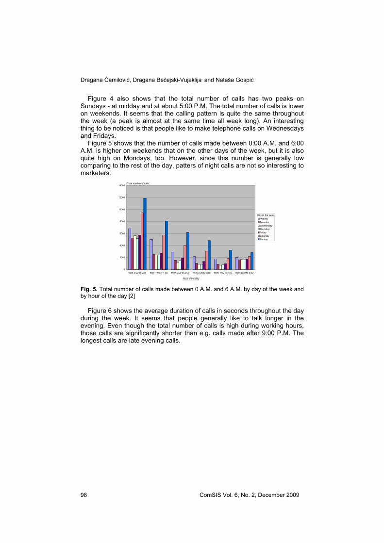
Figure 5 shows that the number of calls made between 0:00 A.M. and 6:00 A.M. is higher on weekends that on the other days of the week, but it is also quite high on Mondays, too. However, since this number is generally low comparing to the rest of the day, patters of night calls are not so interesting to marketers.

0

2000

4000

6000

8000

10000

12000

14000

from 0:00 to 0:59 from 1:00 to 1:59 from 2:00 to 2:59 from 3:00 to 3:59 from 4:00 to 4:59 from 5:00 to 5:59



Hour of the day

Day of the week

Fig. 5. Total number of calls made between 0 A.M. and 6 A.M. by day of the week and by hour of the day [2]

Figure 6 shows the average duration of calls in seconds throughout the day during the week. It seems that people generally like to talk longer in the evening. Even though the total number of calls is high during working hours, those calls are significantly shorter than e.g. calls made after 9:00 P.M. The longest calls are late evening calls.



0

20

40

60

80

100

120

140

160

180fro

m 0

:00

to 0

:59

from

1:0

0 to

1:5

9

from

2:0

0 to

2:5

9

from

3:0

0 to

3:5

9

from

4:0

0 to

4:5

9

from

5:0

0 to

5:5

9

from

6:0

0 to

6:5

9

from

7:0

0 to

7:5

9

from

8:0

0 to

8:5

9

from

9:0

0 to

9:5

9

from

10:

00 to

10:

59

from

11:

00 to

11:

59

from

12:

00 to

12:

59

from

13:

00 to

13:

59

from

14:

00 to

14:

59

from

15:

00 to

15:

59

from

16:

00 to

16:

59

from

17:

00 to

17:

59

from

18:

00 to

18:

59

from

19:

00 to

19:

59

from

20:

00 to

20:

59

from

21:

00 to

21:

59

from

22:

00 to

22:

59

from

23:

00 to

23:

59


Avg call duration

Hour of the day

Day of the week

Fig. 6. Average duration of calls (expressed in seconds) by day of the week and by hour of the day [2]

3.2. Gender and Age Analysis

Figure 7 shows the mobile phone number ownership by gender. Evidentially, there are more male than female subscribers. Only 25% of all subscribers are women. This is important marketing information, and it helps in developing appropriate marketing campaigns. Women should definitely be targeted by a special campaign. Special offer on Mother’s day, for example, could be a good idea.

75%

25%

FM

Number of phone no

Gender

Fig. 7. Phone number ownership by gender [2]

Since there are more male subscribers than female subscribers, the total

number of calls made by men is expected to be higher than the total number of calls made by women (as it is displayed in Figure 8). However, both



genders have similar calling behaviours: calls are increasing in the morning, reaching the peak through middle of the day, and declining in the afternoon. The total number of calls is low in the evening, no matter the gender.

0

100000

200000

300000

400000

500000

600000

700000

800000

from

0:0

0 to

0:5

9

from

1:0

0 to

1:5

9

from

2:0

0 to

2:5

9

from

3:0

0 to

3:5

9

from

4:0

0 to

4:5

9

from

5:0

0 to

5:5

9

from

6:0

0 to

6:5

9

from

7:0

0 to

7:5

9

from

8:0

0 to

8:5

9

from

9:0

0 to

9:5

9

from

10:

00 to

10:

59

from

11:

00 to

11:

59

from

12:

00 to

12:

59

from

13:

00 to

13:

59

from

14:

00 to

14:

59

from

15:

00 to

15:

59

from

16:

00 to

16:

59

from

17:

00 to

17:

59

from

18:

00 to

18:

59

from

19:

00 to

19:

59

from

20:

00 to

20:

59

from

21:

00 to

21:

59

from

22:

00 to

22:

59

from

23:

00 to

23:

59

FM


Hour of the day

Gender

Fig. 8. Total number of calls by gender and by hour of the day [2]

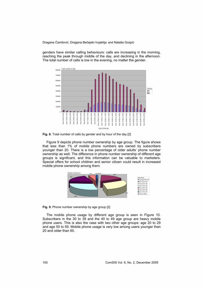
Figure 9 depicts phone number ownership by age group. The figure shows that less than 1% of mobile phone numbers are owned by subscribers younger than 20. There is a low percentage of older adults’ phone number ownership as well. The difference in phone number ownership of different age groups is significant, and this information can be valuable to marketers. Special offers for school children and senior citizen could result in increased mobile phone ownership among them.

16%

31%

29%

19%

4% 1% 0% 0%

younger than 20from 20 to 29from 30 to 39from 40 to 49from 50 to 59from 60 to 69from 70 to 7980 and older

Number of phone no

Age group

Fig. 9. Phone number ownership by age group [2]

The mobile phone usage by different age group is seen in Figure 10. Subscribers in the 30 to 39 and the 40 to 49 age group are heavy mobile phone users. This is also the case with two other age groups: age 20 to 29 and age 50 to 59. Mobile phone usage is very low among users younger than 20 and older than 60.



0

50000

100000

150000

200000

250000

300000

350000fro

m 0

:00

to 0

:59

from

1:0

0 to

1:5

9

from

2:0

0 to

2:5

9

from

3:0

0 to

3:5

9

from

4:0

0 to

4:5

9

from

5:0

0 to

5:5

9

from

6:0

0 to

6:5

9

from

7:0

0 to

7:5

9

from

8:0

0 to

8:5

9

from

9:0

0 to

9:5

9

from

10:

00 to

10:

59

from

11:

00 to

11:

59

from

12:

00 to

12:

59

from

13:

00 to

13:

59

from

14:

00 to

14:

59

from

15:

00 to

15:

59

from

16:

00 to

16:

59

from

17:

00 to

17:

59

from

18:

00 to

18:

59

from

19:

00 to

19:

59

from

20:

00 to

20:

59

from

21:

00 to

21:

59

from

22:

00 to

22:

59

from

23:

00 to

23:

59



Hour of the day

Age group

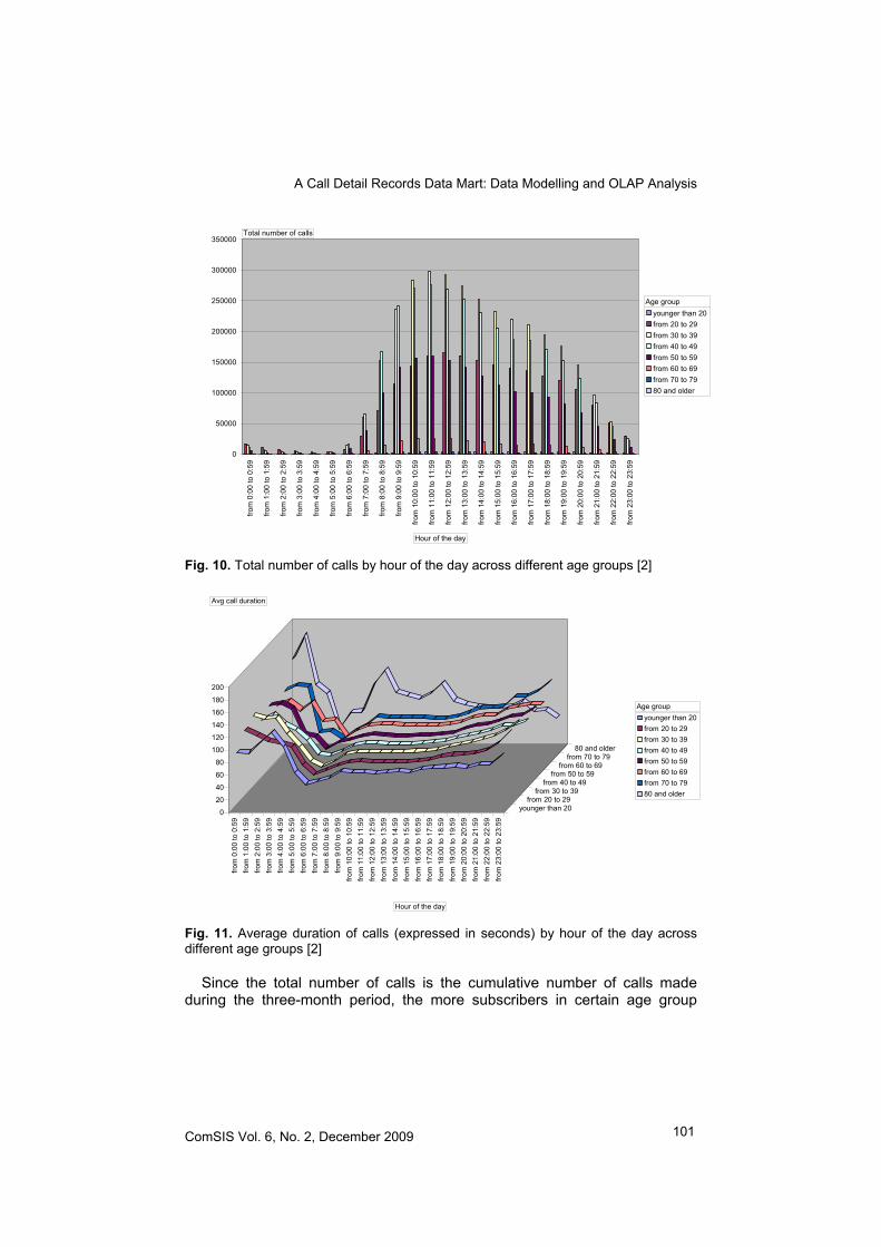
Fig. 10. Total number of calls by hour of the day across different age groups [2]

0

20

40

60

80

100

120

140

160

180

200

from

0:0

0 to

0:5

9fro

m 1

:00

to 1

:59

from

2:0

0 to

2:5

9fro

m 3

:00

to 3

:59

from

4:0

0 to

4:5

9fro

m 5

:00

to 5

:59

from

6:0

0 to

6:5

9fro

m 7

:00

to 7

:59

from

8:0

0 to

8:5

9fro

m 9

:00

to 9

:59

from

10:

00 to

10:

59fro

m 1

1:00

to 1

1:59

from

12:

00 to

12:

59fro

m 1

3:00

to 1

3:59

from

14:

00 to

14:

59fro

m 1

5:00

to 1

5:59

from

16:

00 to

16:

59fro

m 1

7:00

to 1

7:59

from

18:

00 to

18:

59fro

m 1

9:00

to 1

9:59

from

20:

00 to

20:

59fro

m 2

1:00

to 2

1:59

from

22:

00 to

22:

59fro

m 2

3:00

to 2

3:59

younger than 20from 20 to 29

from 30 to 39from 40 to 49

from 50 to 59from 60 to 69

from 70 to 7980 and older


Avg call duration

Hour of the day

Age group

Fig. 11. Average duration of calls (expressed in seconds) by hour of the day across different age groups [2]

Since the total number of calls is the cumulative number of calls made during the three-month period, the more subscribers in certain age group



there are, the higher the total number of calls (although the high frequency of calls, obviously, results in the high total number of calls as well).

Figure 11 shows the average duration of calls in seconds throughout the day by age group. Even though there is less than 1% of mobile phone numbers owned by subscribers older than 80 (see Figure 9), those subscribers generally make longer calls. This could be interesting information for the company in order to provide its older subscribers with optimal service and rate plans. Since the “seniors” tend to talk longer, it would be wise to offer them low cost call rate.

3.3. Rate Plans Analysis

Residential subscribers can choose one of five different post-paid rate plans i.e. tariffs. For the purpose of this study these rate plans are called A, B, C, D and E. They are all listed below. All the charges are expressed in imaginary monetary units (IMU), so that no company is recognizable.

Depending on the rate plan, off-peak minutes could be billed at lower rates. The peak hours are Monday through Friday from 8:00 A.M. to 9:00 P.M.. Weekends and holidays are off-peak hours all day.

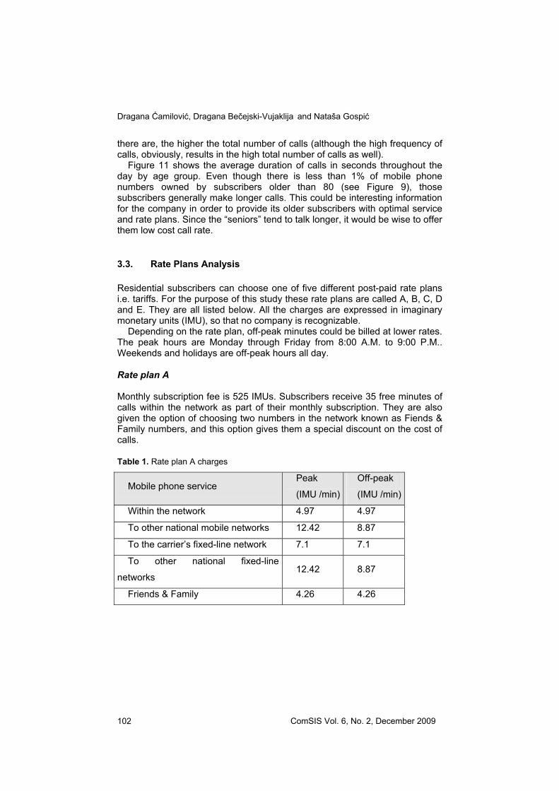
Rate plan A Monthly subscription fee is 525 IMUs. Subscribers receive 35 free minutes of calls within the network as part of their monthly subscription. They are also given the option of choosing two numbers in the network known as Fiends & Family numbers, and this option gives them a special discount on the cost of calls.

Table 1. Rate plan A charges

Mobile phone service Peak

(IMU /min)

Off-peak

(IMU /min)

Within the network 4.97 4.97

To other national mobile networks 12.42 8.87

To the carrier’s fixed-line network 7.1 7.1

To other national fixed-line

networks 12.42 8.87

Friends & Family 4.26 4.26



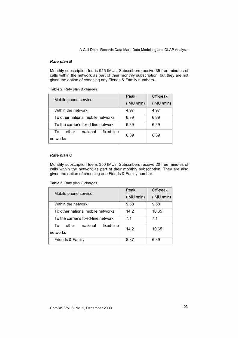
Rate plan B Monthly subscription fee is 945 IMUs. Subscribers receive 35 free minutes of calls within the network as part of their monthly subscription, but they are not given the option of choosing any Fiends & Family numbers.

Table 2. Rate plan B charges


(IMU /min)

Off-peak

(IMU /min)





networks 6.39 6.39

Rate plan C Monthly subscription fee is 350 IMUs. Subscribers receive 20 free minutes of calls within the network as part of their monthly subscription. They are also given the option of choosing one Fiends & Family number.

Table 3. Rate plan C charges


(IMU /min)

Off-peak

(IMU /min)





networks 14.2 10.65




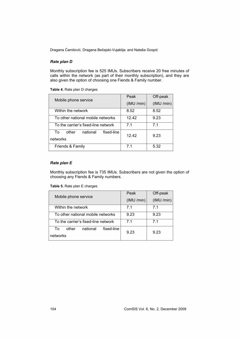
Rate plan D Monthly subscription fee is 525 IMUs. Subscribers receive 20 free minutes of calls within the network (as part of their monthly subscription), and they are also given the option of choosing one Fiends & Family number.

Table 4. Rate plan D charges


(IMU /min)

Off-peak

(IMU /min)





networks 12.42 9.23


Rate plan E Monthly subscription fee is 735 IMUs. Subscribers are not given the option of choosing any Fiends & Family numbers.

Table 5. Rate plan E charges


(IMU /min)

Off-peak

(IMU /min)





networks 9.23 9.23



The share of all the five rate plans is displayed in Figure 12. Rate planes A and B are the new ones, and since they have a growing

share, they are analyzed in detain in the rest of this section.

79%

6%

10%3% 2%

Rate plan ARate plan BRate plan CRate plan DRate plan E

Number of phone no

Rate plan

Fig. 12. Rate plans share

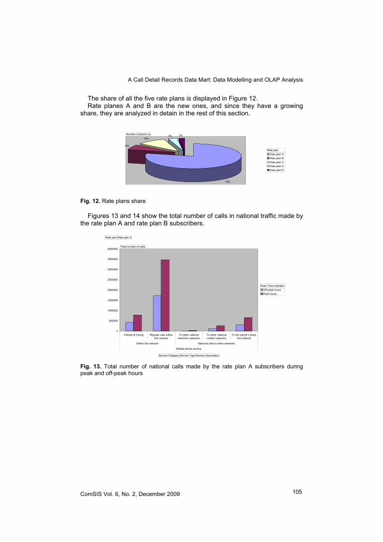
Figures 13 and 14 show the total number of calls in national traffic made by the rate plan A and rate plan B subscribers.

0

500000

1000000

1500000

2000000

2500000

3000000

3500000

4000000

Friends & Family Regular calls withinthe network

To other nationalfixed-line networks

To other nationalmobile networks

To the carrier’s fixed-line network

Within the network National calls to other networks

Mobile phone service

Off-peak hoursPeak hours

Rate plan Rate plan A


Service Category Service Type Service Description

Peak Time Indicator

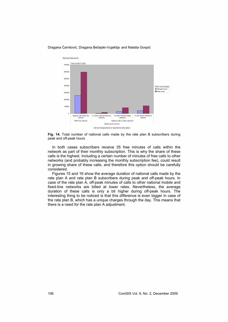
Fig. 13. Total number of national calls made by the rate plan A subscribers during peak and off-peak hours



0

100000

200000

300000

400000

500000

600000

700000

Regular calls within thenetwork

To other national fixed-linenetworks

To other national mobilenetworks

To the carrier’s fixed-linenetwork




Rate plan Rate plan B



Peak Time Indicator

Fig. 14. Total number of national calls made by the rate plan B subscribers during peak and off-peak hours

In both cases subscribers receive 35 free minutes of calls within the network as part of their monthly subscription. This is why the share of these calls is the highest. Including a certain number of minutes of free calls to other networks (and probably increasing the monthly subscription fee), could result in growing share of these calls, and therefore this option should be carefully considered.

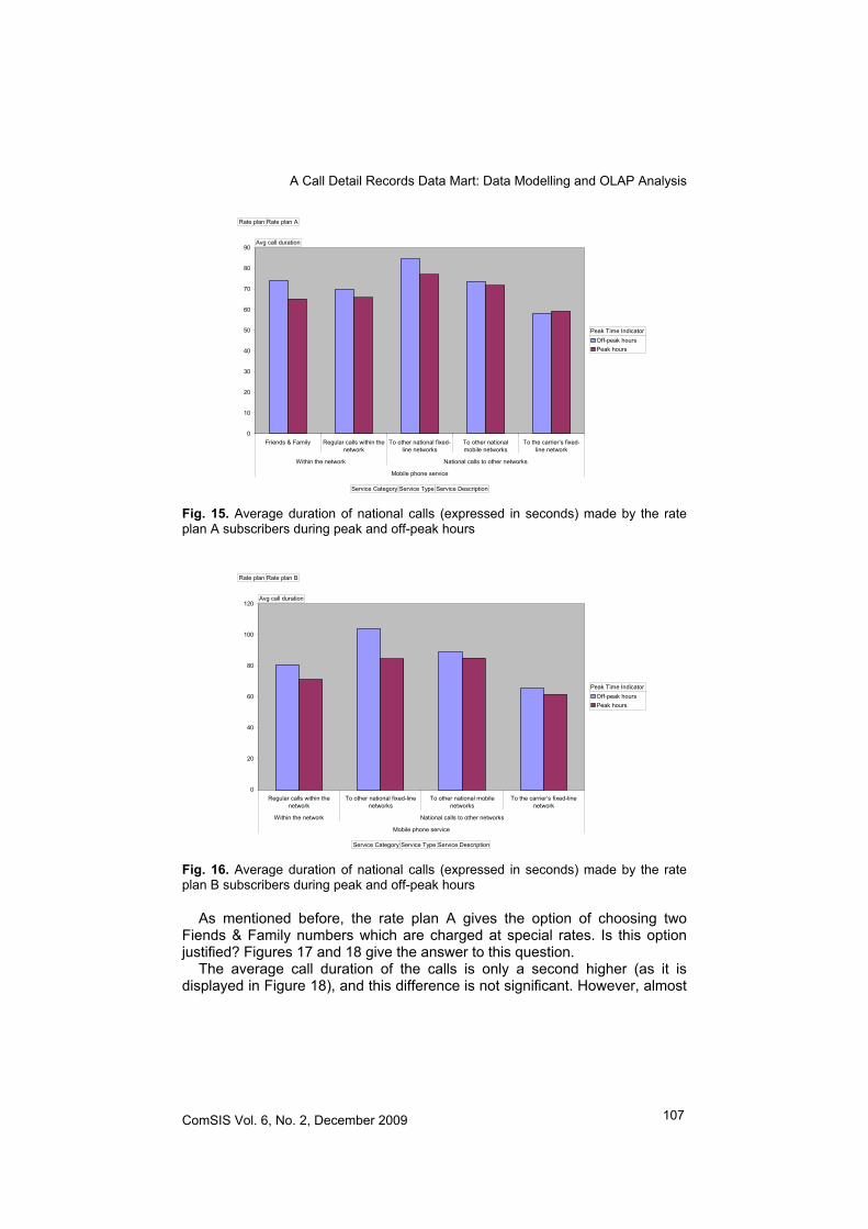
Figures 15 and 16 show the average duration of national calls made by the rate plan A and rate plan B subscribers during peak and off-peak hours. In case of the rate plan A, off-peak minutes of calls to other national mobile and fixed-line networks are billed at lower rates. Nevertheless, the average duration of these calls is only a bit higher during off-peak hours. The interesting thing to be noticed is that this difference is even bigger in case of the rate plan B, which has a unique charges through the day. This means that there is a need for the rate plan A adjustment.



0

10

20

30

40

50

60

70

80

90

Friends & Family Regular calls within thenetwork

To other national fixed-line networks

To other nationalmobile networks

To the carrier’s fixed-line network





Avg call duration


Peak Time Indicator

Fig. 15. Average duration of national calls (expressed in seconds) made by the rate plan A subscribers during peak and off-peak hours

0

20

40

60

80

100

120

Regular calls within thenetwork

To other national fixed-linenetworks

To other national mobilenetworks

To the carrier’s fixed-linenetwork




Rate plan Rate plan B

Avg call duration


Peak Time Indicator

Fig. 16. Average duration of national calls (expressed in seconds) made by the rate plan B subscribers during peak and off-peak hours

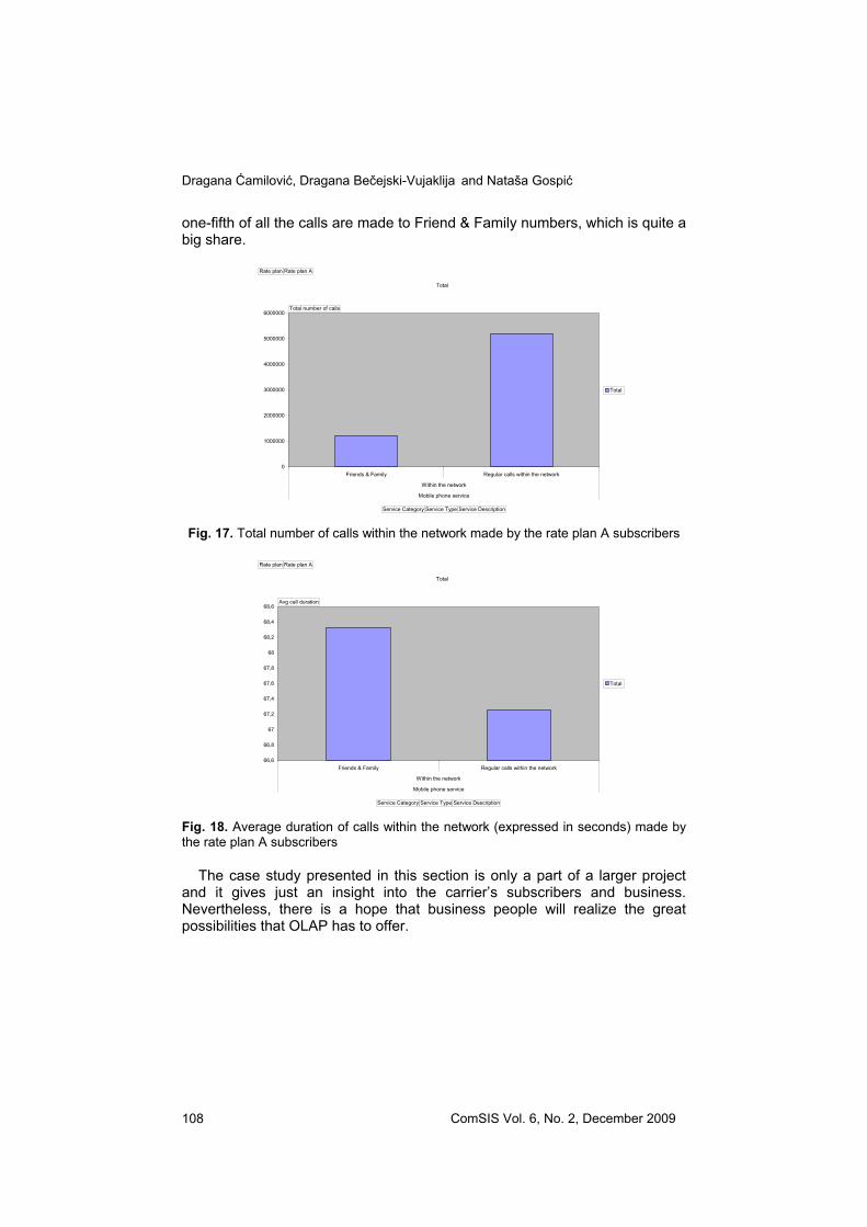
As mentioned before, the rate plan A gives the option of choosing two Fiends & Family numbers which are charged at special rates. Is this option justified? Figures 17 and 18 give the answer to this question.

The average call duration of the calls is only a second higher (as it is displayed in Figure 18), and this difference is not significant. However, almost



one-fifth of all the calls are made to Friend & Family numbers, which is quite a big share.

Total

0

1000000

2000000

3000000

4000000

5000000

6000000

Friends & Family Regular calls within the network

Within the network


Total



Service Category Service Type Service Description Fig. 17. Total number of calls within the network made by the rate plan A subscribers

Total

66,6

66,8

67

67,2

67,4

67,6

67,8

68

68,2

68,4

68,6

Friends & Family Regular calls within the network

Within the network


Total


Avg call duration

Service Category Service Type Service Description Fig. 18. Average duration of calls within the network (expressed in seconds) made by the rate plan A subscribers

The case study presented in this section is only a part of a larger project and it gives just an insight into the carrier’s subscribers and business. Nevertheless, there is a hope that business people will realize the great possibilities that OLAP has to offer.



4. Conclusion

Today, most telecommunications companies collect and refine massive amounts of data, and call detail analysis is one of the hottest areas of exploration in the telecommunications industry. This is why data modelling for the CDR data mart was very interesting to research.

It is very important to design a conceptual model which is easy to understand even to nontechincal users, because end users (i.e. business users) take an active part in defining the business requirements and, therefore, conceptual modelling. The paper describes the CDR data mart dot model in detail. This model is the foundation of the star schema used in the case study presented.

To increase the value of current information resources, OLAP tools can be used. Call detail records can be used in conjunction with demographic data in order to obtain better and more valuable results. The data can be put together and analyzed by using an OLAP cube. The cube can be used for many different purposes: rate plans adjustments, marketing campaign development and pricing improvement. The implementation presented in this paper illustrates all of the above.

5. References

1. Ballard C., Farrell D.M., Gupta A., Mazuela C., Vohnik S., Dimensional Modeling: In a Business Intelligence Environment, International Business Machines Corporation (2006), [Online] Available: http://www.redbooks.ibm.com/redbooks/ pdfs/sg247138.pdf (current January 2009)

2. Camilovic D., A Call Detail Analysis – Getting Insight into Customer Behavior, Tenth Annual International Conference of the Global Business and Technology Association, Madrid, pp. 183-190. (2008)

3. Camilovic D., Data Warehouse as Support for Telecommunications Services Customer Relationship Management, Ph.D. Thesis, Faculty of Organizational Sciences, University of Belgrade, Belgrade (2008)

4. Conceptual, Logical, And Physical Data Models, [Online] Available: http://www.1keydata.com/datawarehousing/data-modelling-levels.html (current January 2009)

5. Grcar M., Mladenic D., Grobelnik M., User Profiling for the Web, Computer Science and Information Systems (ComSIS), Belgrade, Vol. 3, No. 2 (2006)

6. Kimball R, A Dimensional Modeling Manifesto, Miller Freeman Inc., San Francisco (1997), [Online] Available: http://www.dbmsmag.com/9708d15.html (current January 2009)

7. Kimball R., Kimball Design Tip #51: Latest Thinking On Time Dimension Tables, Ralph Kimball Associates, Inc (2004), [Online] Available: http://kimballgroup.com/html/designtipsPDF/KimballDT51LatestThinking.pdf (current January 2009)

8. Kimball R., Ross M., The Data Warehouse Toolkit (Second Edition) - the Complete Guide to Dimensional Modeling, John Wiley & Sons, New York (2002)



9. Kimball R., Surrogate Keys - Data Warehouse Architect (DBMS online), Miller Freeman Inc., San Francisco (1998), [Online] Available: http://www.dbmsmag.com/9805d05.html (current January 2009)

10. Lewis C., A Day With Ralph Kimball – Part 2 (2005), [Online] Available: http://blogs.ittoolbox.com/oracle/guide/archives/a-day-with-ralph-kimball-part-2-3641 (current January 2009)

11. Ponniah P., Data Warehousing Fundamentals: A Comprehensive Guide for IT Professionals, John Wiley & Sons, New York (2001)

12. Todman C., Designing a Data Warehouse: Supporting Customer Relationship Management, Prentice Hall, New Jersey (2000)

13. Weiss, G. M.: Data Mining in Telecommunications, Data Mining and Knowledge Discovery, Springer Science, New York, pp.1189-1201. (2005)

Dragana Ćamilović graduated from Faculty of Organizational Sciences, University of Belgrade in 2001. She got her M.Sc. degree in Information Systems from the same faculty in 2005 and obtained her Ph.D. degree in the year 2008. She is an assistant professor at Faculty of Entrepreneurial Management, Novi Sad. Her research interests include information systems, decision support systems, business intelligence, data warehousing and data mining. She has published a number of scientific papers in the area. Dragana Bečejski-Vujaklija is a professor of IT management at the Department of Information Systems and Technology, Faculty of Organizational Sciences, University Belgrade, Serbia. Her current research areas are IS management and implementation (IT Project management, Procedure making, System performance setup and harmonizing, User training), as well as research in field of ITIL and IT Service Management. Her current projects are in the field of Executive information systems and Business Intelligence system development. She is also the editor-in-chef of a national vocational journal. Nataša Gospić received the B.Sc. and M.Sc. degree from the University of Belgrade, Faculty of Electrical Engineering and PhD degree from the Faculty of Transport and Traffic Engineering. She used to work in telecom sector for more then 30 years as Assistant to General Manager of Community of Yugoslav PTT, General Manager of Mobile operator MONET, Advisor to Director General Telekom Srpske in charge for strategic issues, and member of Managing board of Community of YPTT. She is professor on University Belgrade and Banja Luka. Also, she was a vice chairperson of ITU-D SG 2, responsible for Guidelines dealing with transition to IMT-2000. She is the author of three books, more that 100 scientific and expert papers, editor of ITU handbook on New Technologies and New Services and she was lecturer on more then 35 workshops and seminars organized by International Telecommunication Union from Geneva in developing countries around the globe.

Received: February 13, 2009; Accepted: July 22, 2009.

cdr sample data model

Documents