CDF Formulation for Solving an Optimal Reinsurance Problem

Chengguo Weng∗, and Shengchao Zhuang

Department of Statistics and Actuarial Science

University of Waterloo, Waterloo, Ontario, N2L 3G1, Canada

July 28, 2015

Abstract

An innovative cumulative distribution function (CDF) based method is proposed for

deriving optimal reinsurance contracts for an insurer to maximize its survival probabil-

ity. The optimal reinsurance model is a non-convex constrained stochastic optimization

problem, and the CDF based method transforms it into a linear problem of determining

an optimal CDF over a corresponding feasible set. Compared to the existing literature,

our proposed CDF formulation provides a more transparent derivation of the optimal solu-

tions, and more interestingly, it enables us to solve a further complex model with an extra

background risk.

Key Words: CDF formulation, Lagrangian dual method, optimal reinsurance, survival prob-

ability maximization, background risk.

∗Corresponding author. Tel: +001(519)888-4567 ext. 31132.

Email: Weng (c2weng@uwaterloo.ca), Zhuang (s2zhuang@uwaterloo.ca).

1 Model Setup

1.1 Preliminaries

Let (Ω,F,P) be a probability space, where all the random variables in this paper are dened.

We consider a constrained non-convex stochastic optimal decision problem from an insurance

context. The problem is formulated from the perspective of an insurance company (insurer).

We assume that the insurer has an initial capital of W and is subject to a loss X, which is

a nonnegative random variable with a support of [0,M ] for some M ∈ (0,∞]. For the case

of M = ∞, the support of X is interpreted as [0,∞), and throughout the paper, we assume

E[X] <∞.

The stochastic optimization problem considered in the paper is to determine an optimal

reinsurance purchase strategy against the risk X for the insurer to maximize its survival prob-

ability. Mathematically, it is to nd an optimal partition on X into f(X) and r(X) so that

X = f(X) + r(X), where f : [0,M ] → [0,M ] is a measurable function and so is r. In their

economic meanings, f(X) represents the portion of loss that is ceded to a reinsurer, and r(X)

is the residual loss retained by the insurer. In the context of optimal reinsurance, the ceded

loss function f is often restricted to the set C as given below for the solution (Cui, et al., 2013;

Zheng, et al., 2015):

C :=f(·) : 0 6 f(x) 6 x and r(x) := x− f(x) is non-decreasing ∀ x ∈ [0,M ]

. (1)

The non-decreasing assumption on the retained loss function r is imposed to reduce the moral

hazard risk. If the retained function r is not non-decreasing, the insurer may encourage the

policyholders to claim more so as to reduce its own retained loss but increase the ceded loss on

the reinsurer.

In exchange for covering partial risk for the insurer, the reinsurer charges a premium on the

insurer as compensation. Generally, this premium is always positive, and computed according

to a certain premium principle Π so that the reinsurance premium is given by Π(f(X)). In

our work, we consider the expected value principle and compute the reinsurance premium by

Π(f(X)) = (1 + ρ)E[f(X)], where ρ > 0 is the loading factor.

1.2 Optimal Reinsurance Model in Absence of Background Risk

From the preceding subsection, the insurer's net wealth in the presence of a reinsurance is

given by

T := W − r(X)− (1 + ρ)E[f(X)], (2)

and the insurer is subject to a survival probability of

P(W − r(X)− (1 + ρ)E[f(X)] > 0).

Thus, with the reinsurance premium constrained on a level of π > 0, the optimal reinsurance

problem of maximizing the above survival probability is equivalent to the following one:

2

Problem 1.1 maxf∈C

P(W − r(X)− π > 0

),

s.t. (1 + ρ)E[f(X)] = π,(3)

where π is a reinsurance premium budget satisfying 0 < π ≤ (1 + ρ)E[X].

The research of optimal reinsurance has remained a fascinating area since the seminar

papers Borch (1960) and Arrow (1963), where explicit solutions were derived for minimizing the

variance of the insurer's retained loss (or equivalently the variance of T in (2)) and maximizing

the expected utility of its terminal wealth T respectively, subject to a given net reinsurance

premium of E[f(X)]. These two classic results have been extended in a number of important

directions. Just to name a few, Gajek and Zagrodny (2000) and Kaluszka (2001) generalized

Borch's result by considering the standard deviation premium principle and a class of general

premium principles, respectively. Young (1999) generalized Arrow's result by assuming Wang's

premium principle. Among the recent studies on optimal reinsurance, risk measures including

VaR and CVaR have been extensively used; see, for instance, Cai, et al. (2008), Balbás, et al.,

(2009), Tan, et al. (2009), Tan, et al. (2011), Cheung (2010), Chi and Tan (2013), Asimit, et

al. (2013), Chi and Weng (2013), Cheung, et al. (2014).

1.3 Optimal Reinsurance Model in Presence of Background Risk

In the insurance practice, there are some risks which are not insurable and can potentially

occur with other insurable risks. Moreover, the administration fee on the insurer to settle

insurance claims is often not fully deterministic, and not insured. We generally refer to the

aggregate of these risks which occur along with the underlying risk X as background risk, and

model the risk by a nonnegative random variable Y .

The optimal decision problems with background risk in an insurance context have been in-

tensively studied, but most of these are within a utility maximization framework. For example,

Gollier (1996) considered the optimal insurance purchase strategy by maximizing the expected

utility of a policyholder. For another example, Dana and Scarsini (2007) characterized the

optimal risk sharing strategy between two parties, both being expected utility maximizers. In

the literature, it is common to assume that the background risk is statistically independent

of the insurable risk X, because such assumption leads to much more tractable models and it

works as good approximation in the presence of week dependence. For example, Mahul (2000),

Gollier and Pratt (1996), Courbage et al. (2007), and Schlesinger (2013).

Taking the background risk into account, we compute the terminal net wealth of the insurer

as

W − r(X)− Y − (1 + ρ)E[f(X)],

and accordingly the optimal reinsurance model of maximizing the survival probability goes as

follows:

3

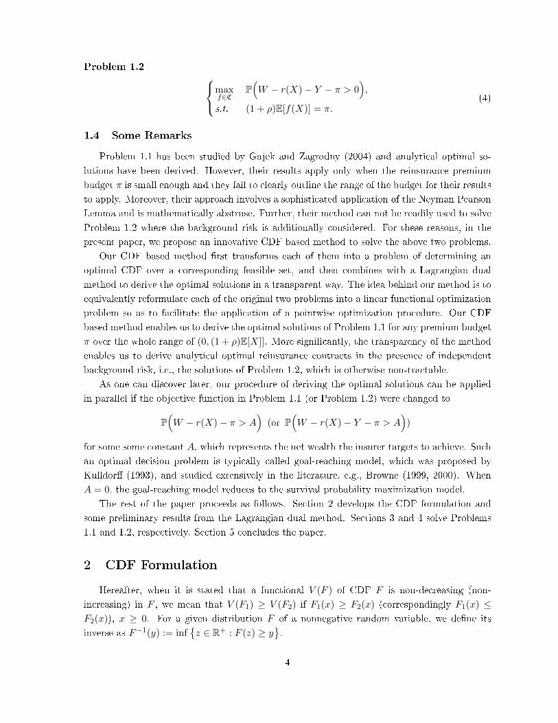
Problem 1.2 maxf∈C

P(W − r(X)− Y − π > 0

),

s.t. (1 + ρ)E[f(X)] = π.(4)

1.4 Some Remarks

Problem 1.1 has been studied by Gajek and Zagrodny (2004) and analytical optimal so-

lutions have been derived. However, their results apply only when the reinsurance premium

budget π is small enough and they fail to clearly outline the range of the budget for their results

to apply. Moreover, their approach involves a sophisticated application of the Neyman Pearson

Lemma and is mathematically abstruse. Further, their method can not be readily used to solve

Problem 1.2 where the background risk is additionally considered. For these reasons, in the

present paper, we propose an innovative CDF based method to solve the above two problems.

Our CDF based method rst transforms each of them into a problem of determining an

optimal CDF over a corresponding feasible set, and then combines with a Lagrangian dual

method to derive the optimal solutions in a transparent way. The idea behind our method is to

equivalently reformulate each of the original two problems into a linear functional optimization

problem so as to facilitate the application of a pointwise optimization procedure. Our CDF

based method enables us to derive the optimal solutions of Problem 1.1 for any premium budget

π over the whole range of (0, (1 + ρ)E[X]]. More signicantly, the transparency of the method

enables us to derive analytical optimal reinsurance contracts in the presence of independent

background risk, i.e., the solutions of Problem 1.2, which is otherwise non-tractable.

As one can discover later, our procedure of deriving the optimal solutions can be applied

in parallel if the objective function in Problem 1.1 (or Problem 1.2) were changed to

P(W − r(X)− π > A

)(or P

(W − r(X)− Y − π > A

))

for some some constant A, which represents the net wealth the insurer targets to achieve. Such

an optimal decision problem is typically called goal-reaching model, which was proposed by

Kulldor (1993), and studied extensively in the literature, e.g., Browne (1999, 2000). When

A = 0, the goal-reaching model reduces to the survival probability maximization model.

The rest of the paper proceeds as follows. Section 2 develops the CDF formulation and

some preliminary results from the Lagrangian dual method. Sections 3 and 4 solve Problems

1.1 and 1.2, respectively. Section 5 concludes the paper.

2 CDF Formulation

Hereafter, when it is stated that a functional V (F ) of CDF F is non-decreasing (non-

increasing) in F , we mean that V (F1) ≥ V (F2) if F1(x) ≥ F2(x) (correspondingly F1(x) ≤F2(x)), x ≥ 0. For a given distribution F of a nonnegative random variable, we dene its

inverse as F−1(y) := infz ∈ R+ : F (z) ≥ y

.

4

Denote

R := r(·) : r(x) ≡ x− f(x) ∀x ∈ [0,M ], f ∈ C.

Then, it follows from (1) that

R =r(·) : r(0) = 0, 0 6 r(x) 6 x ∀x ∈ [0,M ], r(x) is non-decreasing on [0,M ]

,

and thus, Problem 1.1 can be equivalently rewritten, in terms of retained loss function r, as

follows: maxr∈R

P(r(X) ≤W − π

),

s.t. E[r(X)] = π,(5)

where π := E[X]−π/(1 +ρ) and 0 ≤ π < E[X] for 0 < π ≤ (1 +ρ)E[X]. From the formulation

of (5), a necessary condition to have a nonempty feasible set for (5) is given by 0 ≤ π ≤ E[X],

and a trivial solution in the case of π = E[X] is given by r(x) = x, x ∈ [0,M ].

We can similarly rewrite Problem 1.2, in terms of retained loss functions, as follows:maxr∈R

P(r(X) + Y ≤W − π

),

s.t. E[r(X)] = π.(6)

Once a solution, say r∗, is obtained for (5) (or (6)), then f∗(x) := x− r∗(x), x ∈ [0,M ], is

a solution to Problem 1.1 (correspondingly Problem 1.2). Thus, we shall focus on studying (5)

and (6) for optimal solutions.

The following two assumptions will be used in the rest of the paper.

Assumption 2.1 Both the left and right derivatives of the CDF FX(x) of X exist and are

strictly positive over [0,M ].

Assumption 2.2 Y has a non-increasing probability density function gY (·), and is statistically

independent of X.

Remark 1 (a) Assumption 2.1 allows the random variable X to have a probability mass of p

at 0, which is a common model for an insurance loss. Assumption 2.1 is certainly satised if

X has a piecewise continuous density function over (0,M ]. The assumption also implies that

FX is continuous and strictly increasing over [0,M ].

(b) Assumption 2.1 also implies, by the Inverse Function Theorem, that both the left and

right derivatives of F−1X exist and are strictly positive, which we respectively denote by

(F−1X )′−(u) and (F−1X )′+(u), u ∈ (0, 1).

(c) Furthermore, it is worth noting that a great number of typical distributions for insurance

loss modelling satisfy Assumption 2.2, such as Pareto distribution, exponential distribution and

so on.

5

Notably, (6) reduces to (5) if we set Y = 0 almost surely. Nevertheless, our CDF method for

solving (6) relies on Assumption 2.2, whereas the condition of Y = 0 almost surely contradicts

to Assumption 2.2. Therefore, the solution of (5) can not be directly retrieved from that of

(6). We need to analyze both problems separately.

To solve (5) and (6), we reformulate each of them into a problem of identifying an optimal

CDF over a feasible set, and recover the optimal ceded loss functions for the original problems

(5) and (6) from those identied optimal CDF's via Lemma 2.2 in the sequel.

To proceed, we dene

F∗ :=F (·) : F (·) is the CDF of r(X), r ∈ R

,

and

F∗∗ :=F (·) : F (·) is a CDF with F (t) ≥ FX(t) ∀ 0 ≤ t ≤M

. (7)

The equivalence between these two sets of F∗ and F∗∗ is shown in Lemma 2.1 below.

Lemma 2.1 Assume that Assumption 2.1 holds, then F∗ = F∗∗.

Proof. On one hand, for every r ∈ R, r(x) ≤ x ∀ x ∈ [0,M ] and thus we must have

P(r(X) ≤ x) ≥ FX(x) ∀ x ∈ [0,M ]. This means F∗ ⊆ F∗∗. On the other hand, for any

F ∈ F∗∗, we dene r(s) = F−1(FX(s)) for s ∈ [0,M ] to get 0 ≤ r(s) ≤ s, where the second

inequality follows from the fact that F (x) ≥ FX(x) ∀ x ∈ [0,M ]. Moreover, Since FX is

continuous and strictly increasing over [0,M ] due to Assumption 2.1, for any t ∈ [0,M ], there

exists y ∈ [0,M ] such that F (t) = FX(y). Hence, we obtain P(r(X) ≤ t

)= P

(F−1(FX(X)) ≤

t)

= P(FX(X) ≤ F (t)

)= P

(FX(X) ≤ FX(y)

)= P(X ≤ y) = F (t) by Assumption 2.1 again.

This means that F ∈ F∗, and thus, F∗ ⊆ F∗∗.

It is obvious that the reinsurance premium budget constraint E[r(X)] = π in problems (5)

and (6) is equivalent to ∫ M

0

(1− Fr(t)

)dt = π,

where Fr denotes the CDF of r(X). Moreover, the objective in (5) is Fr(W − π), which also

merely depends on the CDF of r(X). Such observation motivates us to consider the following

CDF formulation maxF∈F∗∗

U0(F ) := F (W − π),

s.t.∫M0

(1− F (t)

)dt = π.

(8)

For (6) where the background risk is considered, we apply Assumption 2.2 to rewrite its

objective function as follows

P(r(X) + Y ≤W − π

)=

∫ W−π

0P(r(X) ≤W − π − s

)dFY (s)

6

=

∫ W−π

0P(r(X) ≤ t

)gY (W − π − t)dt.

=

∫ W−π

0Fr(t)gY (W − π − t)dt,

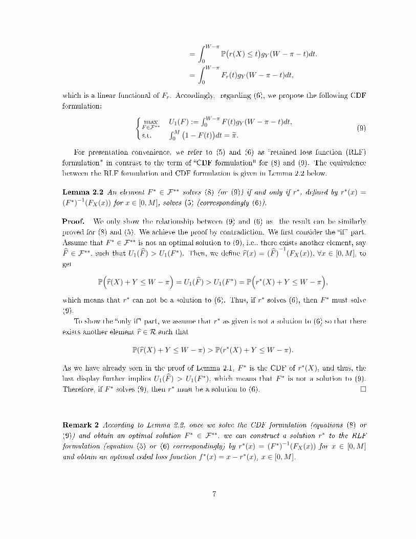
which is a linear functional of Fr. Accordingly, regarding (6), we propose the following CDF

formulation: maxF∈F∗∗

U1(F ) :=∫W−π0 F (t)gY (W − π − t)dt,

s.t.∫M0

(1− F (t)

)dt = π.

(9)

For presentation convenience, we refer to (5) and (6) as retained loss function (RLF)

formulation" in contrast to the term of CDF formulation" for (8) and (9). The equivalence

between the RLF formulation and CDF formulation is given in Lemma 2.2 below.

Lemma 2.2 An element F ∗ ∈ F∗∗ solves (8) (or (9)) if and only if r∗, dened by r∗(x) =

(F ∗)−1(FX(x)) for x ∈ [0,M ], solves (5) (correspondingly (6)).

Proof. We only show the relationship between (9) and (6) as the result can be similarly

proved for (8) and (5). We achieve the proof by contradiction. We rst consider the if part.

Assume that F ∗ ∈ F∗∗ is not an optimal solution to (9), i.e., there exists another element, say

F ∈ F∗∗, such that U1(F ) > U1(F∗). Then, we dene r(x) = (F )

−1(FX(x)), ∀x ∈ [0,M ], to

get

P(r(X) + Y ≤W − π

)= U1(F ) > U1(F

∗) = P(r∗(X) + Y ≤W − π

),

which means that r∗ can not be a solution to (6). Thus, if r∗ solves (6), then F ∗ must solve

(9).

To show the only if" part, we assume that r∗ as given is not a solution to (6) so that there

exists another element r ∈ R such that

P(r(X) + Y ≤W − π) > P(r∗(X) + Y ≤W − π).

As we have already seen in the proof of Lemma 2.1, F ∗ is the CDF of r∗(X), and thus, the

last display further implies U1(F ) > U1(F∗), which means that F ∗ is not a solution to (9).

Therefore, if F ∗ solves (9), then r∗ must be a solution to (6).

Remark 2 According to Lemma 2.2, once we solve the CDF formulation (equations (8) or

(9)) and obtain an optimal solution F ∗ ∈ F∗∗, we can construct a solution r∗ to the RLF

formulation (equation (5) or (6) correspondingly) by r∗(x) = (F ∗)−1(FX(x)) for x ∈ [0,M ]

and obtain an optimal ceded loss function f∗(x) = x− r∗(x), x ∈ [0,M ].

7

In view that the objectives and constraints in (8) and (9) are all linear functionals of the

decision variable F and the feasible set F∗∗ is convex, we exploit the Lagrangian dual method

to solve both problems. This entails introducing a Lagrangian multiplier λ and considering the

following auxiliary problem

maxF∈F∗∗

V0(λ, F ) := F (W − π) + λ(∫ M

0

(1− F (t)

)dt− π

)(10)

for (8), and another auxiliary problem

maxF∈F∗∗

V1(λ, F ) :=

∫ W−π

0F (t)gY (W − π − t)dt+ λ

(∫ M

0

(1− F (t)

)dt− π

)(11)

for (9). Once (10) (or (11)) is solved with an optimal solution Fλ(·) for each λ ∈ R, one can

determine λ∗ ∈ R by solving∫ 10 (1 − Fλ∗(t))dt = π. Then, we can show that F ∗ := Fλ∗ is an

optimal solution to (8) (or (9)) as in Lemma 2.3 below.

Lemma 2.3 Assume that for every λ ∈ R, Fλ(·) solves (10) (or (11)) and there exists a

constant λ∗ ∈ R satisfying∫M0 (1 − Fλ∗(t))dt = π. Then, F ∗ := Fλ∗ solves (8) (or (9) corre-

spondingly).

Proof. We generally denote the objective in (8) (or (9)) by U(F ), and let u(π) denotes its

optimal value. Then, it follows

u(π) = maxF∈F∗∗∫M

0 (1−F (t))dt=π

U(F ) = maxF∈F∗∗∫M

0 (1−F (t))dt=π

[U(F ) + λ∗

(∫ M

0(1− F (t))dt− π

)]

≤ maxF∈F∗∗

[U(F ) + λ∗

(∫ M

0(1− F (t))dt− π

)]=U(F ∗) ≤ u(π),

which implies that F ∗ is optimal to (8) (or (9)).

3 Solutions to Problem 1.1

In this section, we study the optimal solutions when there is no background risk, i.e. the

solutions to Problem 1.1. We analyze the solutions in two scenarios separately (W − π ≥ M

and W −π < M), depending on the relative magnitude of W −π and M . When M =∞, only

the case of W − π < M is possible.

We rst consider the case with W − π ≥ M , where for any feasible f ∈ C we have P(W −r(X)− π > 0) ≥ F (r(X) < M) ≥ FX(M) = 1. Therefore, every element in the feasible set of

Problem 1.1 satisfying the constraint is a solution. We summarize this result in Theorem 3.1

below.

8

Theorem 3.1 Assume that Assumption 2.1 and W−π ≥M hold. Then, any f∗ ∈ C satisfying

(1 + ρ)E[f∗(X)] = π is an optimal ceded loss function to Problem 1.1.

In the rest of the section, we assume W − π < M , which is automatically satised for

M =∞, i.e., X has an unbounded support of [0,∞). According to the analysis in the preceding

section, we can solve the CDF formulation (8) and apply Lemma 2.2 to get the optimal retained

loss function and the optimal ceded loss function. By virtue of Lemma 2.3, we can rst analyze

the solution of (10) for each λ. To this end, we note that

F (W − π) ∈ [FX(W − π), 1] for every F ∈ F∗∗

and consider the following sub-problems

maxF∈F∗∗

V0(λ, F ) := u+ λ(∫ M

0

[1− F (t)

]dt− π

), s.t. F (W − π) = u, (12)

indexed by u ∈ [FX(W − π), 1]. If we could derive an optimal solution F ∗λ,u and get optimal

value ξ(u) := V0(λ, F∗λ,u) of (12) for each u ∈∈ [FX(W −π), 1], then F ∗λ := F ∗λ,u∗ is an optimal

solution to (10), where

u∗ = argmaxu∈[FX(W−π),1]

ξ(u).

Let q = F−1X (u) for u ∈ [FX(W − π), 1]. Since W − π > 0 and FX(x) is continuous and strictly

increasing on [0,M ] according to Assumption 2.1, we have u = FX(q) and q ∈ [W − π,M ].

Thus,

u∗ = FX(q∗) with q∗ = argminq∈[W−π,M ]

ξ(FX(q)).

In the subsequent analysis, we follow such a procedure to solve (10) for λ = 0 and λ > 0,

respectively. Its solution for λ < 0 is not relevant when we invoke Lemma 2.3 for the optimal

CDF of (8) and thus omitted.

Case 3.1 λ = 0.

In this case, the objective in (12) is independent of F and ξ(u) = u, and thus,

the solution to (12) F ∗λ can be any F ∈ F∗∗ which satises F (W − π) = 1. (13)

Case 3.2 λ > 0.

In this case, V0(λ, F ) is non-increasing in F , and the pointwise smallest CDF F ∈ F∗∗ whichsatises F (W − π) = u solves (12). Therefore, from the denition of F∗∗ in (7), a solution to

(12) is given by

F ∗λ,u(t) =

FX(t), if 0 ≤ t < W − π,

u, if W − π ≤ t < F−1X (u),

FX(t), if F−1X (u) ≤ t ≤M,

(14)

9

and as a consequence,

ξ(u) = V0(λ, F∗r(X),u)

= u+ λ

∫ W−π

0(1− FX(t))dt+ λ

∫ F−1X (u)

W−π(1− u)dt+ λ

∫ M

F−1X (u)

(1− FX(t))dt− λπ.

By taking the left derivative of ξ(u), we obtain

ξ′−(u) =1 + λ[ ∫ F−1

X (u)

W−π(−1)dt+ (F−1X )′−(u)(1− FX(F−1X (u))

]=− λ(F−1X )′−(u)

[1− FX(F−1X (u))

]=λ[1 + λ(W − π)

λ− F−1X (u)

], u ∈ [FX(W − π), 1]

We can similarly derive its right derivative, and indeed, it is the same as its left derivative

obtained in the above. This means that ξ(u) is dierentiable over [FX(W − π), 1) with

ξ′(u) = λ[1+λ(W−π)

λ − F−1X (u)], which is decreasing in u. This further implies that ξ(u) is a

concave function of u and attains its maximum at

u∗ = max

FX(W − π), FX

(1 + λ(W − π)

λ

)= FX

(1 + λ(W − π)

λ

).

Thus, one solution to (10) is given by F ∗λ = F ∗λ,u∗ as dened in (14).

With the analysis in the above Cases 3.1 and 3.2, we readily apply Lemma 2.3 to analyze

the solutions to the CDF formulation (8). Denote

π0 =

∫ W−π

0

(1− FX(t)

)dt. (15)

Then, depending on the magnitude of π relative to π0, the optimal solution of (8) can be

obtained as summarized in Proposition 3.1 below.

Proposition 3.1 Assume that Assumption 2.1 and W − π < M hold.

(a) If 0 ≤ π ≤ π0, then one optimal CDF to (8) is given by

F ∗(t) =

FX(t), if 0 ≤ t < t0,

1, if t0 ≤ t ≤M,(16)

where t0 ∈ [0,W − π] is such that∫M0

(1− F ∗(t)

)dt = π.

(b) If π0 < π < E[X], then one CDF to (8) is given by

F ∗(t) =

FX(t), if 0 ≤ t < W − π,

FX(t0), if W − π ≤ t < t0,

FX(t), if t0 ≤ t ≤M,

10

where t0 ∈ [W − π,M ] is such that∫M0

(1− F ∗(t)

)dt = π.

Proof. (a) Given π ∈ [0, π0], there obviously exists a constant t0 ∈ [0,W − π] for F ∗(t)

dened in (16) to satisfy∫M0

(1−F ∗(t)

)dt = π, and F ∗ satises the condition (13). Therefore,

by Lemma 2.3, F ∗ as given by (16) is one solution to (8).

(b) For a ∈ [W − π,M ], dene

Fa(t) :=

FX(t), if 0 ≤ t < W − π,

FX(a), if W − π ≤ t < a,

FX(t), if a ≤ t ≤M,

and q(a) :=∫M0

[1 − Fa(t)

]dt. Obviously, q(a) is a continuous and non-increasing function

of a with q(W − π) = E[X] and q(M) = π0. Therefore, for any π ∈ (π0,E[X]), there exists

t0 ∈ (W − π,M ] such that q(t0) = π which means Ft0 solves (10) for t0 = [1 + λ(W − π)]/λ,

i.e., λ = 1/[t0 − (W − π)], as previously shown in Case 3.2. Thus, the desired result follows

from Lemma 2.3.

The optimal ceded loss functions for the case of W − π < M can be consequently obtained

by combining Proposition 3.1 and Lemma 2.2, and we summarize the results in Theorem 3.2

below.

Theorem 3.2 Assume that Assumption 2.1 and W − π < M hold.

(a) If (1 + ρ)(E[X] − π0) ≤ π ≤ (1 + ρ)E[X], then one optimal cede loss function to Problem

1.1 is given by

f∗(t) =

0, if 0 ≤ t < t0,

t− t0, if t0 ≤ t ≤M,

where t0 is such that (1 + ρ)E[f∗(X)] = π.

(b) If 0 < π < (1 + ρ)(E[X]− π0), then one optimal ceded loss function to Problem 1.1 is given

by

f∗(t) =

0, if 0 ≤ t < W − π,

t− (W − π), if W − π ≤ t < t0,

0, if t0 ≤ t ≤M,

where t0 is such that (1 + ρ)E[f∗(X)] = π.

Proof. Since π = E[X]− π/(1 + ρ), the conditions on π given in both parts are equivalent to

those two in terms of π in Proposition 3.1 respectively, whereby the desired results follow from

11

Proposition 3.1 and Lemma 2.2.

Remark 3 Part (b) of Theorem 3.2 indicates that an truncated stop-loss reinsurance is optimal

for reinsurance premium budget smaller than (1 + ρ)(E[X] − π). The optimality of truncated

stop-loss reinsurance has been established in the Corollary 1 of Gajek and Zagrodny (2004) for

the same Problem 1.1. However, as we have commented in section 1.4, their derivation of

the solution involves a complicated application of Neyman Pearson Lemma, and much more

mathematically abstruse than our CDF method. Furthermore, Gajek and Zagrodny (2004) fail

to identify the range of premium budget π for such a solution as clearly as we do in Theorem

3.2. They also fail to discover the optimality of a stop-loss reinsurance for the case of large

premium budget as stipulated in part (a) of Theorem 3.2.

4 Solutions to Problem 1.2

In this section, we study the optimal solutions when the insurer has a background risk, i.e.,

the solutions of Problem 1.2 or equivalently (6). Based on our analysis in section 2, we need to

solve (9) and apply Lemma 2.2 to get the optimal ceded loss functions. To solve (9), we rst

investigate the solutions of (11) and consequently invoke Lemma 2.3 for optimal reinsurance

contracts. Similar to Section 3, the analysis is divided into two cases of W − π ≥ M and

W − π < M .

4.1 Assume W − π ≥M .

In this case, we can rewrite the objective function in (11) as follows

V (λ, F ) =

∫ M

0F (t)

[gY (W − π − t)− λ

]dt+ 1− FY (W − π −M) + λ(M − π).

Hence, (11) reduces to

maxF∈F∗∗

∫ M

0F (t)

[gY (W − π − t)− λ

]dt+ 1− FY (W − π −M) + λ(M − π), (17)

of which one optimal solution follows from (7) as follows

F ∗λ (t) =

FX(t), if 0 ≤ t ≤M and gY (W − π − t)− λ < 0,

any constant, if 0 ≤ t ≤M and gY (W − π − t)− λ = 0,

1, if 0 ≤ t ≤M and gY (W − π − t)− λ > 0,

(18)

provided that F ∗λ is an appropriate CDF in F∗∗.With an aid of Assumption 2.2 and Lemma 2.3, we can obtain a solution to (9) as given in

Proposition 4.1 below.

12

Proposition 4.1 Suppose that Assumptions 2.1 and 2.2 hold and W − π ≥ M is satised.

Then, one optimal solution to (9) is given by

F ∗(t) =

FX(t), if 0 ≤ t < t0,

1, if t0 ≤ t ≤M,(19)

where t0 is such that∫ t00 [1− F ∗(t)]dt = π.

Proof. For a ∈ [0,M ], we dene

Fa(t) :=

FX(t), if 0 ≤ t < a,

1, if a ≤ t ≤M,

and q(a) :=∫M0

[1− Fa(t)

]dt. Obviously, q(a) is a continuous and non-decreasing function of

a with q(0) = 0 and q(M) = E[X]. Thus, for any π ∈ [0, E[X]), we can nd t0 such that

q(t0) = π. Let λ∗ = gY (W −π− t0). Then, by virtue of Lemma 2.3, F ∗ given in (19) solves (9)

if we could show that it is a solution to (17) for λ = λ∗. Indeed, since gY (W − π − t) is a non-

decreasing function of t, we have gY (W−π−t)−λ∗ ≤ 0 for t ∈ [0, t0) and gY (W−π−t)−λ∗ ≥ 0

for t ∈ (t0,M ], whereby it follows from (18) that F ∗ is a solution to (17) for λ = λ∗. Thus, the

proof is complete.

By invoking Lemma 2.2, we can derive an optimal ceded loss function to solve Problem 1.2.

Theorem 4.1 Assume that Assumptions 2.1 and 2.2 hold and W − π ≥ M is satised. One

optimal solution to Problem 1.2 is given by

f∗(x) =

0, if 0 ≤ x < t0,

x− t0, if t0 ≤ x ≤M,(20)

where t0 is determined by (1 + ρ)E[f∗(X)] = π.

Proof. It is a direct consequence of Proposition 4.1 and Lemma 2.2.

4.2 Assume W − π < M .

In this case, the objective function in (11) can be rewritten as follows

V1(λ, F ) =

∫ W−π

0F (t)

[gY (W − π − t)− λ

]dt− λ

∫ M

W−πF (t)dt+ λ(M − π). (21)

13

We follow the same procedure as applied in Section 3 to solve (11). Because F (W − π) ∈[FX(W − π), 1] for every F ∈ F∗∗, we consider the following sub-problems

maxF∈F∗∗

V1(λ, F ), s.t. F (W − π) = u, (22)

indexed by u ∈ [FX(W −π), 1]. If we could derive an optimal solution F ∗λ,u and optimal value

η(u) := V1(λ, F∗λ,u) of (22) for each for each u ∈∈ [FX(W − π), 1], then F ∗λ := F ∗λ,u∗ with

u∗ = argmaxu∈[FX(W−π),1]

η(u) is an optimal solution to (11).

We analyze the solutions of (22) for λ, respectively, in three dierent ranges: λ = 0,

0 < λ ≤ gY ((W − π)−), and gY ((W − π)−) ≤ λ ≤ gY (0+). The case of λ > gY (0+) is not

relevant in order to apply Lemma 2.3 for optimal CDF of (9) and thus omitted.

Case 4.1 λ = 0.

From (21), in this case, V1(λ, F ) =∫W−π0 F (t)gY (W − π − t)dt, which is non-decreasing in

F . Therefore, F ∗λ (t) = 1, t ∈ [0,M ], is an optimal solution to (11).

Case 4.2 0 < λ ≤ gY ((W − π)−).

In this case, gY (W − π − t) ≥ λ for t ∈ [0,W − π]. Therefore, by virtue of (21), a solution

to (22) is given by

F ∗λ,u(t) =

u, if 0 ≤ t < F−1X (u),

FX(t), if F−1X (u) ≤ t ≤M,

which, along with the condition u ∈ [FX(W − π), 1], further implies

η(u) := V1(λ, F∗λ,u)

=

∫ W−π

0u[gY (W − π − t)− λ

]dt− λ

∫ F−1X (u)

W−πudt− λ

∫ M

F−1X (u)

FX(t)dt+ λ(M − π).

We compute the left derivative of η(u) as follows

η′−(u) =

∫ W−π

0

[gY (W − π − t)− λ

]dt− λ

[∫ F−1X (u)

W−πdt+ u · (F−1X )′−(u)

]+ λFX(F−1X (u))(F−1X )′−(u)

=λ[FY (W − π)

λ− F−1X (u)

], u ∈ (FX(W − π), 1).

We can similarly derive its right derivative, and indeed, it is the same as the left derivative we

just obtained. Thus, η(u) is dierentiable over u ∈ (FX(W −π), 1) with η′(u) = λ(FY (W−π)

λ −

F−1X (u)), which is decreasing in u. This implies that η(u) is a concave function for u ∈

[FX(W − π], 1] and attains its maximum over [FX(W − π), 1] at

u∗ = min

max

[FX(W − π), FX

(FY (W − π)

λ

)], 1

.

14

We further note that

FY (W − π) =

∫ W−π

0gY (y)dy ≥

∫ W−π

0gY ((W − π)−)dy = (W − π)gY ((W − π)−),

and thus, FY (W − π)/λ ≥W − π for 0 < λ ≤ gY ((W − π)−). This implies

u∗ = min

FX

(FY (W − π)

λ

), 1

= FX

(min

(FX(W − π)

λ, M

)),

and

F ∗λ (t) = F ∗λ,u∗(t) =

FX(

min(FX(W−π)

λ , M))

, if 0 ≤ t < min(FX(W−π)

λ , M),

FX(t), if min(FX(W−π)

λ , M)≤ t ≤M.

Notably, in the case of M ≤ FX(W − π)/λ, F ∗λ (t) = 1 for t ∈ [0,M ].

Case 4.3 gY ((W − π)−) ≤ λ ≤ gY (0+).

In this case, there exists t0 ∈ [0,W − π] such that gY (W − π− t)− λ ≤ 0 for t ∈ [0, t0) and

gY (W − π − t)− λ ≥ 0 for t ∈ (t0,W − π], where [0, t0) = ∅ for t0 = 0. Hence, in view of (21)

and the fact that F (t) ≥ FX(t), ∀t ∈ [0,M ] and F (W − π) = u for every feasible F in (22), a

solution to (22) is given by

F ∗λ,u(t) =

FX(t), if 0 ≤ t < t0,

u, if t0 ≤ t < F−1X (u),

FX(t), if F−1X (u) ≤ t ≤M.

Accordingly,

η(u) := V1(λ, F∗λ,u)

=

∫ t0

0FX(t)

[gY (W − π − t)− λ

]dt+

∫ W−π

t0

u[gY (W − π − t)− λ

]dt

−λ∫ F−1

X (u)

W−πudt− λ

∫ M

F−1X (u)

FX(t)dt+ λ(M − π).

Similarly to the previous case, we respectively consider the left and right derivatives of η(u)

and nd that they coincide for u ∈ (FX(W − π), 1) and are given by

η′(u) =λ[FY (W − π − t0)

λ+ t0 − F−1X (u)

],

which is non-increasing as a function of u ∈ [FX(W −π), 1]. This implies that η(u) is concave

and attains its maximum over [FX(W − π), 1] at

u∗ = min

max

[FX(W − π), FX

(FY (W − π − t0)λ

+ t0

)], 1

.

15

Since gY (t) is non-increasing in t and gY (W − π − t) ≥ λ for t ∈ (t0,W − π],

FY (W − π − t0)/λ+ t0 =

∫ W−π

t0

gY (W − π − t)λ

dt+ t0 ≥∫ W−π

t0

dt+ t0 = W − π.

Hence,

u∗= min

FX

(FY (W − π − t0)λ

+ t0

), 1

= FX

(min

(FY (W − π − t0)λ

+ t0, M))

=FX (H(t0, λ)) ,

and

F ∗λ (t) = F ∗λ,u∗(t) =

FX(t), if 0 ≤ t < t0,

FX

(H(t0, λ)

), if t0 ≤ t < H(t0, λ),

FX(t), if H(t0, λ) ≤ t ≤M,

(23)

where

H(t, λ) = min

FY (W − π − t)

λ+ t, M

. (24)

With the analysis in the above Cases 4.1, 4.2 and 4.3, Lemma 2.3 can be readily invoked

for the solution of (11). The solution is given in Propositions 4.2 and 4.3, respectively, for a

small π and a large π. To proceed, we dene

d := FY (W − π)/gY ((W − π)−) and φ(F ) :=

∫ M

0[1− F (t)] dt, F ∈ F∗∗. (25)

We further write

π1 :=

∫ d

0[1− FX(t)] dt. (26)

Proposition 4.2 Assume that Assumptions 2.1 and 2.2 hold. For 0 ≤ d ≤M , dene

Fd(t) :=

FX(d), if 0 ≤ t < d,

FX(t), if d ≤ t ≤M.

Then, for each π ∈ [0, π1], there exists a constant t0 ∈[d, M

]to satisfy φ(Ft0) = π and Ft0

solves (9).

Proof. Based on the analysis in Case 4.1, Fd solves (11) with λ = FY (W − π)/d,

d ∈[d, M

]. Moreover, it is easy to check that φ(Fd) is continuous as a function of d with

limd→M φ(Fd) = 0 and limd→d φ(Fd) = φ(F

d) = π1. Thus, by the Intermediate Value Theorem,

16

there exists a constant t0 ∈[d, M

]such that φ(Ft0) = π, and consequently, by Lemma 2.3,

Ft0 is one solution to (9).

To derive the solution to (9) for π larger than π1, some extra notations are necessary. For

each a ∈ [0,W − π], we denote

Λa :=

[limt→a+

gY (W − π − t), limt→a−

gY (W − π − t)].

Further, for each a ∈ [0,W − π] and λa ∈ Λa, we dene

F (a,λa)(t) :=

FX(t), if 0 ≤ t < a,

FX

(H(a, λa)

), if a ≤ t < H(a, λa),

FX(t), if H(a, λa) ≤ t ≤M,

(27)

so that

φ(F (a,λa)) =

∫ a

0[1− FX(t)] dt+ [H(a, λa)− a] · [1− FX(H(a, λa))]

+

∫ M

H(a,λa)[1− FX(t)] dt.

Since gY (t) is non-increasing in t, given any λ ∈ Λa, gY (W −π− t)−λ ≤ 0 for t ∈ [0, a) and

gY (W−π−t)−λ ≥ 0 for t ∈ (a,W−π]. Therefore, according to the analysis in Case 4.3, F(a,λa)

is a solution to (22) for any λa ∈ Λa. Moreover, it is worth noting that Λa = gY (W −π− a),which is a singleton set, at any continuity point a of gY (W − π− a). Therefor, for any interval

(s1, s2) where gY (W − π − t) is continuous, φ(F (a,λa)) is a continuous function of a.

Proposition 4.3 Assume that Assumptions (2.1) and (2.2) hold. For each

π ∈ [π1, E[X]) ,

there exists a constant a ∈ [0,W − π] and λa ∈ Λa such that F (a,λa) solve (9).

Proof. Based on the analysis in Case 4.3 and Lemma 2.3, it is sucient to show the

existence of a ∈ [0,W −π] and λa ∈ Λa to satisfy φ(F (a,λa)) = π for each π ∈ [π1, E[X]). Note

that F (a,λa) = Fdfor a = 0 and λa = limt→0+ gY (W−π−t) = gY ((W−π)−), and F (a,λa) = FX

for a = W − π and any λa ∈ ΛW−π. These two cases lead to φ(F (a,λa)) = φ(Fd) = π1 and

φ(F (a,λa)) = E[X], respectively. Therefore, it is sucient for us to assume π ∈ (π1, E[X]) in

the rest of the proof.

Dene

Sπ :=t ∈ [0,W − π] : ∃λ ∈ Λt such that φ(F (t,λt)) > π

,

17

and t0 := supSπ. If gY (W−π−t) is continuous at t0, then it is continuous over a neighbourhoodof t0, say (t0 − δ, t0 + δ) for some constant δ > 0, because it is a monotone function. In this

case, Λt = g(W − π − t) for each t ∈ (t0 − δ, t0 + δ) and therefore, φ(F (a,λa)) is a continuous

function of a over (t0 − δ, t0 + δ) with λa = g(W − π − a), which in turn implies that, given

any ε > 0,

φ(F (s,λs))− ε ≤ φ(F (t0,λt0 )) ≤ φ(F (s,λs)) + ε,

whenever s ∈ (t0 − κ, t0 + κ) for some constant κ ∈ (0, δ). On one hand, by the supremum

property of t0, there exists s1 ∈ (t0 − δ1, t0) and s1 ∈ Sπ such that

φ(F (t0,λt0 )) ≥ φ(F (s1,λs1 ))− ε ≥ π − ε.

One the other hand, there exists s2 ∈ (t0, t0 + δ2) and s2 /∈ Sπ such that

φ(F (t0,λt0 )) ≤ φ(F (s2,λs2 )) + ε ≤ π + ε.

Letting ε→ 0 in the last two displays, we get φ(F (t0,λt0 )) = π.

Otherwise, we assume that gY (W − π − t) is discontinuous at t0, and dene

g−t0 := limt→t−0

gY (W − π − t), and g+t0 := limt→t+0

gY (W − π − t).

Since gY (W − π − t) is monotone as a function of t, it has at most countably jumps, which

in turn implies that there exists a constant δ > 0 such that gY (W − π − t) is continuous over(t0 − δ, t0) and (t0, t0 + δ). Therefore, φ(F (s,λs)) is a continuous function of s over (t0 − δ, t0)and (t0, t0 + δ) with

lims→t−0

φ(F (s,λs)) = φ(F (t0,g−t0)) and lim

s→t+0φ(F (s,λs)) = φ(F (t0,g

+t0)).

By the supremum property of t0, there exists s1 ∈ (t0 − δ, t0) and s1 ∈ Sπ such that

φ(F (t0,g−t0)) ≥ φ(F (s1,λs1 ))− ε ≥ π − ε.

On the other hand, there exists s2 ∈ (t0, t0 + δ) and s2 /∈ Sπ such that

φ(F (t0,g+t0)) ≤ φ(F (s2,λs2 )) + ε ≤ π + ε.

Letting ε→ 0 in the last two displays, we obtain

φ(F (t0,g+t0)) ≤ π ≤ φ(F (t0,g

−t0)).

φ(F (t0,λ)) with t0 xed is a continuous function of λ and therefore, there must exist some

λt0 ∈ [g+t0 , g−t0

] ≡ Λt0 such that φ(F (t0,λt0 )) = π.

The optimal ceded loss function for Problem 1.2 can be retrieved from the optimal CDF

that is derived in Propositions 4.2 and 4.3 by invoking Lemma 2.2.

18

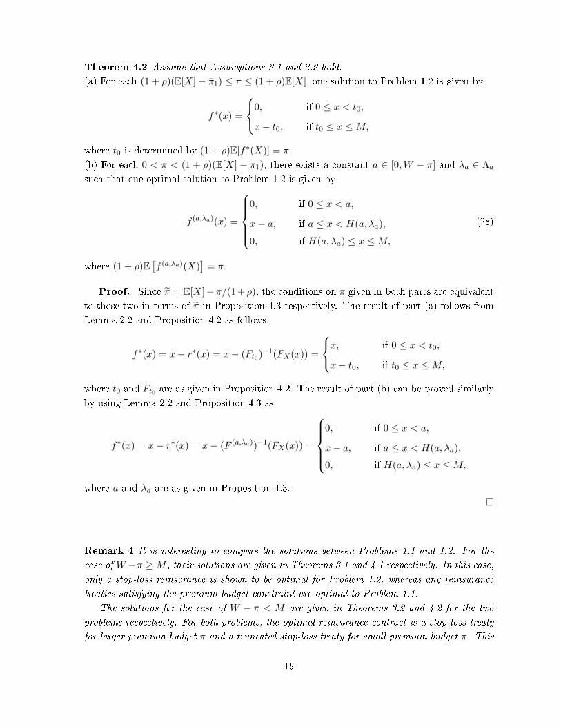
Theorem 4.2 Assume that Assumptions 2.1 and 2.2 hold.

(a) For each (1 + ρ)(E[X]− π1) ≤ π ≤ (1 + ρ)E[X], one solution to Problem 1.2 is given by

f∗(x) =

0, if 0 ≤ x < t0,

x− t0, if t0 ≤ x ≤M,

where t0 is determined by (1 + ρ)E[f∗(X)] = π.

(b) For each 0 < π < (1 + ρ)(E[X] − π1), there exists a constant a ∈ [0,W − π] and λa ∈ Λa

such that one optimal solution to Problem 1.2 is given by

f (a,λa)(x) =

0, if 0 ≤ x < a,

x− a, if a ≤ x < H(a, λa),

0, if H(a, λa) ≤ x ≤M,

(28)

where (1 + ρ)E[f (a,λa)(X)

]= π.

Proof. Since π = E[X]−π/(1 + ρ), the conditions on π given in both parts are equivalent

to those two in terms of π in Proposition 4.3 respectively. The result of part (a) follows from

Lemma 2.2 and Proposition 4.2 as follows

f∗(x) = x− r∗(x) = x− (Ft0)−1(FX(x)) =

x, if 0 ≤ x < t0,

x− t0, if t0 ≤ x ≤M,

where t0 and Ft0 are as given in Proposition 4.2. The result of part (b) can be proved similarly

by using Lemma 2.2 and Proposition 4.3 as

f∗(x) = x− r∗(x) = x− (F (a,λa))−1(FX(x)) =

0, if 0 ≤ x < a,

x− a, if a ≤ x < H(a, λa),

0, if H(a, λa) ≤ x ≤M,

where a and λa are as given in Proposition 4.3.

Remark 4 It is interesting to compare the solutions between Problems 1.1 and 1.2. For the

case of W −π ≥M , their solutions are given in Theorems 3.1 and 4.1 respectively. In this case,

only a stop-loss reinsurance is shown to be optimal for Problem 1.2, whereas any reinsurance

treaties satisfying the premium budget constraint are optimal to Problem 1.1.

The solutions for the case of W − π < M are given in Theorems 3.2 and 4.2 for the two

problems respectively. For both problems, the optimal reinsurance contract is a stop-loss treaty

for larger premium budget π and a truncated stop-loss treaty for small premium budget π. This

19

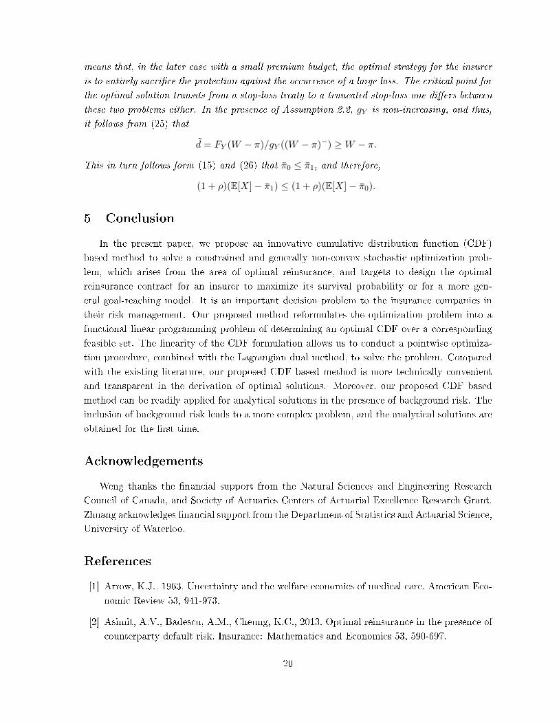
means that, in the later case with a small premium budget, the optimal strategy for the insurer

is to entirely sacrice the protection against the occurrence of a large loss. The critical point for

the optimal solution transits from a stop-loss treaty to a truncated stop-loss one diers between

these two problems either. In the presence of Assumption 2.2, gY is non-increasing, and thus,

it follows from (25) that

d = FY (W − π)/gY ((W − π)−) ≥W − π.

This in turn follows form (15) and (26) that π0 ≤ π1, and therefore,

(1 + ρ)(E[X]− π1) ≤ (1 + ρ)(E[X]− π0).

5 Conclusion

In the present paper, we propose an innovative cumulative distribution function (CDF)

based method to solve a constrained and generally non-convex stochastic optimization prob-

lem, which arises from the area of optimal reinsurance, and targets to design the optimal

reinsurance contract for an insurer to maximize its survival probability or for a more gen-

eral goal-reaching model. It is an important decision problem to the insurance companies in

their risk management. Our proposed method reformulates the optimization problem into a

functional linear programming problem of determining an optimal CDF over a corresponding

feasible set. The linearity of the CDF formulation allows us to conduct a pointwise optimiza-

tion procedure, combined with the Lagrangian dual method, to solve the problem. Compared

with the existing literature, our proposed CDF based method is more technically convenient

and transparent in the derivation of optimal solutions. Moreover, our proposed CDF based

method can be readily applied for analytical solutions in the presence of background risk. The

inclusion of background risk leads to a more complex problem, and the analytical solutions are

obtained for the rst time.

Acknowledgements

Weng thanks the nancial support from the Natural Sciences and Engineering Research

Council of Canada, and Society of Actuaries Centers of Actuarial Excellence Research Grant.

Zhuang acknowledges nancial support from the Department of Statistics and Actuarial Science,

University of Waterloo.

References

[1] Arrow, K.J., 1963. Uncertainty and the welfare economics of medical care. American Eco-

nomic Review 53, 941-973.

[2] Asimit, A.V., Badescu, A.M., Cheung, K.C., 2013. Optimal reinsurance in the presence of

counterparty default risk. Insurance: Mathematics and Economics 53, 590-697.

20

[3] Balbás, A., Balbás, B., Heras, A., 2009. Optimal reinsurance with general risk measures.

Insurance: Mathematics and Economics 44, 374-384.

[4] Borch, K., 1960. An attempt to determine the optimum amount of stop loss reinsurance.

In: Transactions of the 16th International Congress of Actuaries, Vol. I. 597-610.

[5] Browne, S., 1999. Reaching goals by a deadline: digital options and continuous-time active

portfolio management. Advances in Applied Probability 31(2), 551-577.

[6] Browne, S., 2000. Risk-constrained dynamic active portfolio management. Management

Science 46(9), 1188-1199.

[7] Cai, J., Tan, K.S., Weng, C., Zhang, Y., 2008. Optimal Reinsurance under VaR and CTE

Risk Measures. Insurance: Mathematics and Economics 43, 185-196.

[8] Cheung, K.C., 2010. Optimal reinsurer revisited - a geometric approach. ASTIN Bulletin

40, 221-239.

[9] Cheung, K.C., Sung, K.C.J., Yam, S.C.P., Yung, S.P., 2014. Optimal reinsurance under

general law-invariant risk measures. Scandinavian Actuarial Journal 2014(1), 72-91.

[10] Chi, Y., Tan, K.S., 2013. Optimal reinsurance with general premium principles. Insurance:

Mathematics and Economics 52, 180-189.

[11] Chi, Y., Weng, C., 2013. Optimal reinsurance subject to Vajda condition. Insurance: Math-

ematics and Economics 53, 179-189.

[12] Courbage, C.,Rey, B., 2007. Precautionary saving in the presence of other risks. Economic

Theory 32, 417-424.

[13] Cui, W., Yang, J., Wu, L., 2013. Optimal reinsurance minimizing the distortion risk mea-

sure under general reinsurance premium principles. Insurance: Mathematics and Eco-

nomics 53, 74-85.

[14] Dana, R.-A., Scarsini, M., 2007. Optimal risk sharing with background risk. Journal of

Economic Theory 133, 152-176.

[15] Gajek, L., Zagrodny, D., 2000. Insurer's optimal reinsurance strategies. Insurance: Math-

ematics and Economics 27, 105-112

[16] Gajek, L., Zagrodny, D., 2004. Reinsurance arrangements maximizing insurer's survival

probability. Journal of Risk and Insurance 71, 421-435.

[17] Gollier, C., 1996. Optimal insurance approximate losses. The Journal of Risk and Insurance

63, 369-380.

[18] Gollier, C., Pratt, J., 1996. Risk vulnerability and the tempering eect of background risk.

Econometrica 64(5), 1109-1123.

21

[19] Kaluszka, M., 2001. Optimal reinsurance under mean-variance premium principles. Insur-

ance: Mathematics and Economics 28, 61-67.

[20] Kulldor, M., 1993. Optimal control of favorable games with a time limit. SIAM. Journal

of Control and Optimization 31(1), 52-69.

[21] Mahul, O., 2000. Optimal insurance design with random initial wealth. Economics Letters

69, 353-358.

[22] Schlesinger, H., 2013. The theory of insurance demand. In: Handbook of InsuranceNew

York: Springer, 167-184.

[23] Tan, K.S., Weng, C., Zhang, Y., 2009. VaR and CTE criteria for optimal quota-share and

stop-loss reinsurance. North American Actuarial Journal 13, 450-482.

[24] Tan, K.S., Weng, C., Zhang, Y., 2011. Optimality of general reinsurance contracts under

CTE risk measure. Insurance: Mathematics and Economics 49, 175-187.

[25] Young, V.R., 1999. Optimal insurance under Wang's premium principle. Insurance: Math-

ematics and Economics 25, 109-122.

[26] Zheng Y., Wei, C., Yang, J., 2015. Optimal reinsurance under distortion risk measures and

expected value premium principle for reinsurer. Journal of Systems Science and Complexity

28, 122-143.

22