cbo's working paper
TRANSCRIPT
Working Paper Series
Congressional Budget Office
Washington, DC
How CBO Estimates the Effects of the Affordable
Care Act on the Labor Market
Edward Harris
Tax Analysis Division
Congressional Budget Office
Shannon Mok
Tax Analysis Division
Congressional Budget Office
December 2015
Working Paper 2015-09
To enhance the transparency of the work of the Congressional Budget Office and to encourage external
review of that work, CBO’s working paper series includes papers that provide technical descriptions of
official CBO analyses as well as papers that represent independent research by CBO analysts. Papers in
this series are available at http://go.usa.gov/ULE.
For helpful comments and suggestions, the authors thank Jessica Banthin, Linda Bilheimer, Molly Dahl,
Wendy Edelberg, Philip Ellis, Katherine Fritzsche, Keith Hall, Jeffrey Kling, Sarah Masi, Benjamin Page,
Naveen Singhal, Robert Stewart, Robert Sunshine, and David Weiner, all of CBO, as well as the staff of
the Joint Committee on Taxation.
Abstract
The Affordable Care Act (ACA) will make the labor supply, measured as the total compensation paid to
workers, 0.86 percent smaller in 2025 than it would have been in the absence of that law, the
Congressional Budget Office estimates. Three-quarters of that decline will occur because of health
insurance expansions, which raise effective tax rates on earnings from labor—for instance, by phasing out
health insurance subsidies as people’s income rises—and thus reduce the amount of labor that workers
choose to supply. The labor force is projected to be about 2 million full-time-equivalent workers smaller
in 2025 under the ACA than it would have been otherwise. Those estimates were based mainly on CBO’s
calculations of the effects of the law’s major components on marginal and average tax rates and on the
agency’s analysis of research about the change in the labor supply resulting from a change in tax rates.
For components of the law that were difficult to express in terms of changes in tax rates, CBO based its
estimates on a review of the available literature about similar policy changes.
Contents
Summary ....................................................................................................................................................... 1
Overview of CBO’s Methods ....................................................................................................................... 2
Changes in Marginal and Average Tax Rates ........................................................................................ 3
Labor Supply Elasticities ........................................................................................................................ 3
An Illustration ......................................................................................................................................... 5
Effects of Health Insurance Coverage Expansions ....................................................................................... 5
Exchange Subsidies ................................................................................................................................ 6
Rules Governing Insurance .................................................................................................................. 11
Medicaid Expansion ............................................................................................................................. 12
Effects of Taxes and Penalties .................................................................................................................... 14
Hospital Insurance Surtax..................................................................................................................... 14
Employer Mandate and Penalty ............................................................................................................ 14
High-Premium Excise Tax ................................................................................................................... 15
Individual Mandate and Penalty ........................................................................................................... 16
Effects on Total Hours and Full-Time-Equivalent Employment ................................................................ 17
Uncertainty of the Effects ........................................................................................................................... 18
Tables
Table 1. The Effects of the Affordable Care Act on the Supply of Labor in 2025 ....................................... 2
Table 2. Marginal Tax Rates From Premium Assistance Credits, Four-Person Family
With a $9,800 Premium, 2014 ...................................................................................................................... 7
Table 3. Marginal Tax Rates From Cost-Sharing Subsidies and Premium Assistance Credits,
Four-Person Family With a $9,800 Premium, 2014 ..................................................................................... 9
Table 4. CBO’s Labor Supply Elasticities .................................................................................................. 19
Summary
The economic projections that the Congressional Budget Office uses to construct its baseline budget
projections are based partly on the agency’s estimates of how federal policies will affect the economy,
provided that current law does not change. Those federal policies include the Affordable Care Act (ACA),
which makes the supply of labor smaller than it would have been otherwise, CBO estimates. This paper
describes the methods and calculations underlying that estimate.
The paper focuses on CBO’s estimate of labor supply effects in 2025. In that year, CBO estimates, the
ACA will make the labor supply, measured as the total compensation paid to workers, 0.86 percent
smaller than it would have been in the absence of that law. Earlier, in the 2016–2018 period, the estimated
effects of the ACA on the supply of labor will be smaller, mostly because of delays in people’s responses
to changes in law. By 2019, however, the ACA will reduce the labor supply by 0.80 percent, and the
effect will rise slowly to the aforementioned 0.86 percent by 2025, CBO estimates. Because the ACA
affects people who earn lower wages more than it affects people who earn higher wages, the estimated
effect on the labor supply will be larger—a drop of 1.7 percent—if measured by the decline in total hours
worked.
Those estimates reflect CBO’s assessment of how workers, employers, and others will respond to the
many significant changes that the ACA has made to federal programs and tax policies. Some provisions
of the law will raise effective tax rates on earnings from labor—for instance, by phasing out health
insurance subsidies as people’s income rises—and thus reduce the amount of labor that workers choose to
supply. Other provisions will reduce the labor supply by imposing higher taxes on labor income directly;
an example is the ACA’s increase in the payroll tax that high-income workers pay for Medicare’s
Hospital Insurance (HI) program. And the ACA’s health insurance subsidies will make it easier for some
people to work less or stop working without losing health insurance coverage.
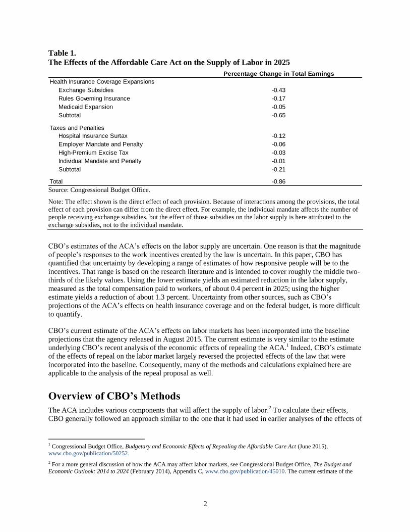
CBO’s current estimate of the ACA’s effect on the labor supply in 2025 is the sum of several components
(see Table 1):
Health insurance coverage expansions—comprising exchange subsidies, rules governing health
insurance, and an expansion of the Medicaid program—are together expected to reduce the labor
supply by 0.65 percentage points.
The HI surtax is expected to reduce the labor supply by 0.12 percentage points.
Other major provisions—a penalty on larger employers that do not offer insurance coverage, an
excise tax on certain high-premium insurance plans, and a penalty on certain individuals who do
not obtain coverage—are together expected to reduce the labor supply by 0.10 percentage point.
The projected reduction in the labor supply would occur in several ways. Some people would choose to
work fewer hours; others would leave the labor force entirely or remain unemployed for longer than they
otherwise would. CBO did not split its estimate of the overall reduction into the reduction in the number
of hours worked and the reduction in labor force participation, because in formulating its estimate, the
agency generally relied on labor supply elasticities (which measure the change in the labor supply
resulting from a change in tax rates) that combined those two decisions. CBO did, however, translate the
reduction in the labor supply into an effect on full-time-equivalent employment. The labor force is
projected to be about 2 million full-time-equivalent workers smaller in 2025 than it would have been
otherwise.
2
Table 1.
The Effects of the Affordable Care Act on the Supply of Labor in 2025
Source: Congressional Budget Office.
Note: The effect shown is the direct effect of each provision. Because of interactions among the provisions, the total
effect of each provision can differ from the direct effect. For example, the individual mandate affects the number of
people receiving exchange subsidies, but the effect of those subsidies on the labor supply is here attributed to the
exchange subsidies, not to the individual mandate.
CBO’s estimates of the ACA’s effects on the labor supply are uncertain. One reason is that the magnitude
of people’s responses to the work incentives created by the law is uncertain. In this paper, CBO has
quantified that uncertainty by developing a range of estimates of how responsive people will be to the
incentives. That range is based on the research literature and is intended to cover roughly the middle two-
thirds of the likely values. Using the lower estimate yields an estimated reduction in the labor supply,
measured as the total compensation paid to workers, of about 0.4 percent in 2025; using the higher
estimate yields a reduction of about 1.3 percent. Uncertainty from other sources, such as CBO’s
projections of the ACA’s effects on health insurance coverage and on the federal budget, is more difficult
to quantify.
CBO’s current estimate of the ACA’s effects on labor markets has been incorporated into the baseline
projections that the agency released in August 2015. The current estimate is very similar to the estimate
underlying CBO’s recent analysis of the economic effects of repealing the ACA.1 Indeed, CBO’s estimate
of the effects of repeal on the labor market largely reversed the projected effects of the law that were
incorporated into the baseline. Consequently, many of the methods and calculations explained here are
applicable to the analysis of the repeal proposal as well.
Overview of CBO’s Methods
The ACA includes various components that will affect the supply of labor.2 To calculate their effects,
CBO generally followed an approach similar to the one that it had used in earlier analyses of the effects of
1 Congressional Budget Office, Budgetary and Economic Effects of Repealing the Affordable Care Act (June 2015),
www.cbo.gov/publication/50252.
2 For a more general discussion of how the ACA may affect labor markets, see Congressional Budget Office, The Budget and
Economic Outlook: 2014 to 2024 (February 2014), Appendix C, www.cbo.gov/publication/45010. The current estimate of the
Health Insurance Coverage Expansions
Exchange Subsidies -0.43
Rules Governing Insurance -0.17
Medicaid Expansion -0.05
Subtotal -0.65
Taxes and Penalties
Hospital Insurance Surtax -0.12
Employer Mandate and Penalty -0.06
High-Premium Excise Tax -0.03
Individual Mandate and Penalty -0.01
Subtotal -0.21
Total -0.86
Percentage Change in Total Earnings
3
federal policies on people’s incentives to work.3 First, CBO calculated the effects of most of the law’s
major components on marginal and average tax rates. The agency then estimated the effects of those
changes in tax rates by applying estimates of labor supply elasticities to them. CBO’s estimates of those
elasticities are drawn from a substantial body of economic research.
However, two components of the law were difficult to express in terms of changes in tax rates. In those
cases, CBO based its estimates on a review of the available literature about similar policy changes.
Specifically, CBO’s estimate of the effect of the Medicaid expansion on the labor supply was based on
several studies of states’ changes in eligibility criteria for Medicaid, and CBO’s estimate of the effect of
health insurance rules and subsidies on people’s retirement decisions was drawn from the literature
studying analogous changes made in the past.
Changes in Marginal and Average Tax Rates
CBO estimated the effects on marginal and average tax rates of three major provisions of the ACA—the
exchange subsidies, the HI surtax, and the high-premium excise tax—using the agency’s tax simulation
model. The model begins with a representative sample of taxpayers, which the agency adjusts to account
for expected demographic and economic changes throughout the next 10 years. Next, CBO calculates
taxes for each member of the sample in two circumstances—one in which a provision of the ACA is in
place, and one in which it is not—to determine the changes in tax rates that result from that provision.4
CBO’s tax simulation model lacks some information needed to estimate the effects of two major
provisions—the employer penalty and the individual penalty—on each taxpayer’s marginal and average
tax rates. The agency therefore made a simplified calculation of those provisions’ total effects on tax
rates. For example, the model does not contain information about the size of the firm that employs each
person in the sample; because the employer penalty depends partly on the size of the employer, that lack
of information makes it impossible to estimate the penalty that a firm would pay if it failed to offer health
insurance coverage to a particular person. So instead of using the model, CBO estimated the total change
in tax rates by combining the total amount of employer penalties that would be paid—which the agency
had previously estimated in conjunction with the staff of the Joint Committee on Taxation (JCT)—with
estimates of the income of workers at firms potentially subject to the penalty.
Labor Supply Elasticities
In deciding how much they will work, people respond to various incentives, including incentives created
by taxes on income from work and incentives created by government benefits that vary with income. To
estimate the effects of the ACA on the labor supply, CBO used elasticities that measure how much the
labor supply changes in response to changes in those incentives. It may take people some time to alter
their work situation in response to changes in incentives; the elasticities are intended to measure people’s
eventual response.
ACA’s effects on labor markets is somewhat smaller than the estimate that the agency used when preparing that report, primarily
because CBO now expects fewer people to receive subsidies through health insurance exchanges.
3 For more details about CBO’s general approach, see Congressional Budget Office, How the Supply of Labor Responds to
Changes in Fiscal Policy (October 2012), www.cbo.gov/publication/43674.
4 For a detailed description of CBO’s tax simulation model and its use in analyzing changes in fiscal policy that affect the labor
supply, see Congressional Budget Office, The Effect of Tax Changes on Labor Supply in CBO’s Microsimulation Tax Model
(April 2007), www.cbo.gov/publication/18554. However, the model now incorporates the estimates of labor supply elasticities
described in this paper, rather than the estimates described in that report.
4
Changes in taxes on labor income can create two different pressures on people’s willingness to work.
Those pressures are known as the substitution effect and the income effect.
Substitution Effect. Many tax changes affect marginal tax rates—the rates that apply to an
additional dollar of a taxpayer’s income. A tax change that raises marginal rates reduces after-tax
compensation for an additional hour of work, making that work less valuable relative to other
uses of a person’s time, so some people will spend less time working and more time on those
other activities. (That is, those people will substitute other activities for work.) By itself, that
substitution effect means that an increase in marginal tax rates reduces the supply of labor.
Income Effect. Tax changes also affect average tax rates—the rates that describe total taxes as a
share of a taxpayer’s income. A tax change that raises average tax rates reduces the after-tax
income that a taxpayer receives from a given amount of work, meaning that the taxpayer has to
work more in order to maintain the same standard of living.5 By itself, that income effect means
that an increase in average tax rates increases the supply of labor.
Substitution elasticities measure the change in the labor supply resulting from a change in the net-of-tax
wage rate—that is, the wages for an additional hour of work that are retained after taxes are paid. The
change in that measure is equivalent to the change in the net-of-tax marginal rate, which is equal to
100 percent minus the marginal tax rate. Similarly, income elasticities measure the change in the labor
supply resulting from a change in after-tax income. That change is equal to the change in the net-of-tax
average rate, which equals 100 percent minus the average tax rate.
Some policies, such as an increase in statutory tax rates, move marginal and average tax rates in the same
direction. When that occurs, the substitution and income effects push labor supply in opposite directions,
and the net result depends on which effect is larger.
Other policies, including the health insurance subsidies provided by the ACA, move marginal and average
tax rates in opposite directions. Consequently, their substitution and income effects push labor supply in
the same direction. Phasing out a benefit as recipients’ income rises effectively increases their marginal
tax rate, discouraging them from working via the substitution effect; and providing the benefit in the first
place effectively increases their income, discouraging them from working via the income effect.
CBO uses separate elasticities to estimate the income and the substitution effects. CBO’s income
elasticity is the same for all workers. But on the basis of a literature review that the agency conducted in
2012, it has developed various estimates of the substitution elasticity for various kinds of workers.6
Specifically, CBO estimates that the substitution elasticity is larger for secondary workers (that is, the
lower-earning spouses in married couples) than for primary workers (a category that comprises the
higher-earning spouses and unmarried people); the agency also estimates that among primary workers, the
substitution elasticity is larger for lower earners than for higher earners. In other words, for a given
percentage change in the return on working an additional hour, the amount of labor supplied by secondary
workers and lower earners will respond more strongly than will the amount of labor supplied by primary
workers and higher earners. CBO’s central estimates of the substitution elasticity range from 0.31 for
5 CBO approximates the change in average tax rates resulting from a policy change by calculating after-tax income as if labor
supply and pretax income were unchanged.
6 For more details, see Congressional Budget Office, How the Supply of Labor Responds to Changes in Fiscal Policy (October
2012), www.cbo.gov/publication/43674; and Robert McClelland and Shannon Mok, A Review of Recent Research on Labor
Supply Elasticities, Working Paper 2012-12 (Congressional Budget Office, October 2012), www.cbo.gov/publication/43675.
5
low-earning primary earners to 0.22 for high-earning primary earners, and the agency’s central estimate
for secondary workers is 0.32.
CBO’s average substitution elasticity for all earners—calculated as the average among subgroups of
workers, with the weight of each subgroup equal to the total earnings of workers in that subgroup—
ranges from 0.16 to 0.32, and the central estimate is 0.24. The agency’s income elasticity ranges from
−0.10 to zero, and the central estimate is −0.05. (An elasticity of zero would mean that no income effect
occurred.) The ranges reflect uncertainty about how people respond to tax changes generally and are
intended to cover roughly the middle two-thirds of the likely values for the elasticities. However, they
may not capture uncertainty about how people will respond to the ACA’s provisions specifically, as this
paper discusses later.
The effects on the labor supply of a change in taxes or benefits can come in two forms. Some people may
choose to continue working but change how many hours they work, which is called a response on the
intensive margin of the labor supply. Other people may choose to enter the labor force or leave it, which
is called responding on the extensive margin. In its current modeling approach, CBO uses substitution and
income elasticities that combine those two forms of response.
A final consideration is that people may not recognize changes in law immediately or alter their work
situation immediately in response to those changes. In this analysis, therefore, CBO phases in the labor
supply effects stemming from the ACA over a three-year period. The main result is to reduce the
estimated labor supply effects during the first three years of the analysis—from 2016 through 2018.
An Illustration
CBO’s method of estimating the effect of a tax change on the labor supply can be illustrated by
considering a hypothetical tax change: a 2 percentage-point tax increase on all income, starting from a
marginal tax rate of 30 percent and an average tax rate of 20 percent. That change would increase the
marginal and average tax rates by 2 percentage points each.
If the marginal tax rate on wages was 30 percent and the average tax rate on all income was 20 percent,
the net-of-tax marginal rate would be 70 percent and the net-of-tax average rate would be 80 percent. A
2 percentage-point tax increase on all income would decrease the net-of-tax marginal rate by 2 percentage
points, or 2.9 percent (2 ÷ 70); that is, people’s after-tax wages for an additional hour of work would be
68 percent of their before-tax wages, rather than 70 percent—2.9 percent less. The tax increase would
likewise decrease the net-of-tax average rate by 2 percentage points, or 2.5 percent (2 ÷ 80).
Those percentage changes would be multiplied by the substitution and income elasticities to yield an
estimate of the percentage change in the labor supply. CBO’s central estimates of the elasticities are 0.24
and −0.05, respectively. So the substitution effect would reduce the labor supply by 0.70 percent
(−2.9 × 0.24), on average, and the income effect would increase the labor supply by 0.13 percent
(−2.5 × −0.05), for a net reduction of 0.57 percent.
Effects of Health Insurance Coverage Expansions
Provisions of the ACA that affect the labor supply may be divided into two groups: those that expand
health insurance coverage and those that impose explicit taxes or penalties related to earnings or
employment. This section of the paper discusses the former.
The ACA expands health insurance coverage by offering subsidies to certain people who purchase
insurance through health insurance exchanges; by establishing rules that make it easier or less expensive
6
for people with higher expected health care costs to obtain coverage; and by expanding eligibility for
Medicaid. CBO estimates that in 2025, about 25 million people, on net, will gain health insurance
coverage as a result of the law. CBO further estimates that those provisions will make the labor supply,
measured as the total compensation paid to workers, 0.65 percent smaller in 2025 than it would have been
otherwise (see Table 1 on page 2). The exchange subsidies will account for most of that effect.
Exchange Subsidies
The ACA’s exchange subsidies come in two forms: premium assistance credits, which defray some of the
costs of people’s health insurance premiums, and cost-sharing subsidies, which reduce their out-of-pocket
expenses for health care. In general, to receive a premium assistance credit, a person must be a U.S.
citizen or legal immigrant; have modified adjusted gross income between 100 percent and 400 percent of
the federal poverty guidelines (commonly known as the federal poverty level, or FPL); not be eligible for
affordable health insurance through another qualifying source, such as an employer, Medicaid, or
Medicare; and purchase insurance through an exchange (where the person’s eligibility is checked).7 To
receive a cost-sharing subsidy, a person must qualify for premium assistance credits and have income
below 250 percent of the FPL.
Both kinds of subsidy increase the resources of recipients, reducing work incentives through the income
effect. In addition, the subsidies decline as income increases, reducing the return on earning additional
income. That decline is effectively an increase in recipients’ effective marginal tax rate, so it generally
reduces their work incentives through the substitution effect. CBO also expects that the subsidies, by
reducing the burden of unemployment, will create additional work disincentives for people who are
unemployed for part of the year. Because of their effects on work incentives, the exchange subsidies will
reduce the aggregate labor supply by 0.43 percent in 2025, CBO estimates.
Premium Assistance Credits. The marginal tax rates implicit in the premium assistance credit schedule
can be quite large, for two reasons: The subsidy amounts are large for the recipients with the lowest
income, and those subsidies are phased out as income rises. In 2014, the first year in which exchange
subsidies were available, a family of four whose income equaled 100 percent of the FPL ($23,550) and
whose premium for a reference plan was $9,800 would have received premium assistance credits worth
about $9,300. (A reference plan is the second-cheapest silver plan offered in an exchange in a person’s
geographic area; silver plans are those that pay about 70 percent of enrollees’ costs for covered benefits,
on average.) But if that family’s income rose past 400 percent of the FPL ($94,200), the subsidy would
fall to zero. Over that income range, the family would thus lose about 13 cents of subsidy per dollar of
additional earnings: $9,300 ÷ ($94,200 − $23,550).
The premium assistance credit that a person receives equals the difference between the premium for that
person’s reference plan and an expected contribution by that person. The person’s expected contribution
rises with income—both because it is calculated as a percentage of income and because that percentage
rises with income. The increase in the expected contribution associated with increases in income (and the
resulting decrease in the subsidy) is similar to a tax on income and thus increases marginal tax rates. The
resulting marginal rate would be added to whatever marginal tax rate the family had faced previously
through the tax and transfer system—on average, about 30 percent for low- and moderate-income
families.8
7 Adjusted gross income (AGI) equals gross income from taxable sources minus certain deductions. Modified AGI equals AGI
plus income earned abroad, tax-exempt Social Security income, and tax-exempt interest income.
8 For more details, see Congressional Budget Office, Effective Marginal Tax Rates for Low- and Moderate-Income Workers in
2016 (November 2015), www.cbo.gov/publication/50923.
7
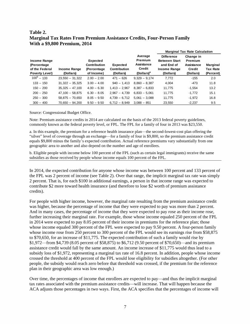
Table 2.
Marginal Tax Rates From Premium Assistance Credits, Four-Person Family
With a $9,800 Premium, 2014
Source: Congressional Budget Office.
Note: Premium assistance credits in 2014 are calculated on the basis of the 2013 federal poverty guidelines,
commonly known as the federal poverty level, or FPL. The FPL for a family of four in 2013 was $23,550.
a. In this example, the premium for a reference health insurance plan—the second-lowest-cost plan offering the
“silver” level of coverage through an exchange—for a family of four is $9,800, so the premium assistance credit
equals $9,800 minus the family’s expected contribution. Actual reference premiums vary substantially from one
geographic area to another and also depend on the number and age of enrollees.
b. Eligible people with income below 100 percent of the FPL (such as certain legal immigrants) receive the same
subsidies as those received by people whose income equals 100 percent of the FPL.
In 2014, the expected contribution for anyone whose income was between 100 percent and 133 percent of
the FPL was 2 percent of income (see Table 2). Over that range, the implicit marginal tax rate was simply
2 percent. That is, for each $100 in additional earnings, a person in that income range was expected to
contribute $2 more toward health insurance (and therefore to lose $2 worth of premium assistance
credits).
For people with higher income, however, the marginal rate resulting from the premium assistance credit
was higher, because the percentage of income that they were expected to pay was more than 2 percent.
And in many cases, the percentage of income that they were expected to pay rose as their income rose,
further increasing their marginal rate. For example, those whose income equaled 250 percent of the FPL
in 2014 were expected to pay 8.05 percent of their income in premiums for the reference plan; those
whose income equaled 300 percent of the FPL were expected to pay 9.50 percent. A four-person family
whose income rose from 250 percent to 300 percent of the FPL would see its earnings rise from $58,875
to $70,650, for an increase of $11,775. The expected contribution of such a family would rise by
$1,972—from $4,739 (8.05 percent of $58,875) to $6,712 (9.50 percent of $70,650)—and its premium
assistance credit would fall by the same amount. An income increase of $11,775 would thus lead to a
subsidy loss of $1,972, representing a marginal tax rate of 16.8 percent. In addition, people whose income
crossed the threshold at 400 percent of the FPL would lose eligibility for subsidies altogether. (For other
people, the subsidy would reach zero before that threshold was crossed, if the premium for the reference
plan in their geographic area was low enough.)
Over time, the percentages of income that enrollees are expected to pay—and thus the implicit marginal
tax rates associated with the premium assistance credits—will increase. That will happen because the
ACA adjusts those percentages in two ways. First, the ACA specifies that the percentages of income will
100b– 133 23,550 – 31,322 2.00 – 2.00 471 – 626 9,329 – 9,174 7,772 -155 2.0
133 – 150 31,322 – 35,325 3.00 – 4.00 940 – 1,413 8,860 – 8,387 4,004 -473 11.8
150 – 200 35,325 – 47,100 4.00 – 6.30 1,413 – 2,967 8,387 – 6,833 11,775 -1,554 13.2
200 – 250 47,100 – 58,875 6.30 – 8.05 2,967 – 4,739 6,833 – 5,061 11,775 -1,772 15.1
250 – 300 58,875 – 70,650 8.05 – 9.50 4,739 – 6,712 5,061 – 3,088 11,775 -1,972 16.8
300 – 400 70,650 – 94,200 9.50 – 9.50 6,712 – 8,949 3,088 – 851 23,550 -2,237 9.5
Difference
Between Start
and End of
Income Range
(Dollars)
Change in
Premium
Assistance
Credit
(Dollars)
Marginal Tax Rate Calculation
Income Range
(Percentage
of the Federal
Poverty Level)
Income Range
(Dollars)
Expected
Contribution
(Percentage
of Income)
Expected
Contribution
(Dollars)
Average
Premium
Assistance
Credit
(Dollars)a
Marginal
Tax Rate
(Percent)
8
increase each year to reflect the difference between average growth in premiums for health insurance and
average growth in household income. For example, if health insurance premiums grew 2 percent faster
than household income each year, on average, the percentages of income to be paid by enrollees would
rise by a factor of 1.02 per year. Second, beginning in 2019, if the total cost of exchange subsidies in the
previous year exceeds 0.504 percent of gross domestic product (GDP), the contribution schedule will be
further indexed to constrain the costs of the subsidies.9
CBO expects growth in health insurance premiums to exceed the rate of income growth per capita by a
substantial margin over the coming decade. CBO also estimates that the total cost of exchange subsidies
may exceed the specified threshold. Combining the two factors, CBO expects that the shares of income
that enrollees will be expected to contribute at any given percentage of the FPL will rise by about one-
fourth between 2014 and 2025. For example, the share of income contributed—and thus the marginal tax
rate—for people whose income is 100 percent to 133 percent of the FPL will rise from 2.0 percent in
2014 to about 2.5 percent in 2025; for people whose income is 300 percent to 400 percent of the FPL, it
will rise from 9.5 percent to about 12 percent.
Cost-Sharing Subsidies. The cost-sharing subsidies offered by the ACA, which are available only to
people who select a silver plan and who have income below 250 percent of the FPL, cover some of the
out-of-pocket costs that those people would otherwise have paid. Because a silver plan is expected to pay
for about 70 percent of its enrollees’ costs for covered benefits, on average—in other words, it has an
actuarial value of about 70 percent—the enrollees are expected to pay 30 percent, on average, out of
pocket. However, the cost-sharing subsidies increase the actuarial value of a silver plan to 94 percent for
enrollees whose income is between 100 percent and 150 percent of the FPL, to 87 percent for enrollees
whose income is between 150 percent and 200 percent of the FPL, and to 73 percent for enrollees whose
income is between 200 percent and 250 percent of the FPL.
Like the premium assistance credits, the cost-sharing subsidies decline as income rises, increasing
recipients’ marginal tax rates. Because the subsidies phase out in steps, declining sharply when recipients’
income exceeds 150 percent, 200 percent, and 250 percent of the FPL, they create “cliffs” at those points,
where the effective marginal tax rate exceeds 100 percent. For example, in 2014, a family of four with an
income exactly equal to 150 percent of the FPL would have received a cost-sharing subsidy worth
roughly $3,038, on average, if it had purchased a silver plan that cost about the national average.10
If the
family’s income had risen by one dollar, that subsidy could have fallen abruptly by about $882 (to about
$2,156), yielding a marginal tax rate well in excess of 100 percent.
The marginal rates stemming from the cost-sharing subsidy can be substantial not only at the cliffs but
over broader income ranges as well.11
For example, if that family’s income rose from 125 percent to
175 percent of the FPL, it would lose about $882 in subsidies (see Table 3). That represents a marginal
tax rate of 7.5 percent over that income range. When that rate was added to the 13.0 percent marginal rate
9 For more details about the indexing provisions, see Congressional Budget Office, Additional Information About CBO’s Baseline
Projections of Federal Subsidies for Health Insurance Provided Through Exchanges (May 2011), www.cbo.gov/
publication/41464.
10 The realized value of the subsidy can vary considerably and depends on how much health care is consumed, but using the
average value allows CBO to estimate the subsidies’ effects on work incentives reasonably well (unless health care spending is
strongly correlated with marginal tax rates or elasticities of labor supply).
11 In estimating the marginal rate effect of the cost-sharing subsidies, CBO has linearly smoothed the schedule; that is, rather than
applying an extremely high rate to the very small number of people who would move past one of the cliffs, the agency has
applied a lower rate to a larger number of people.
9
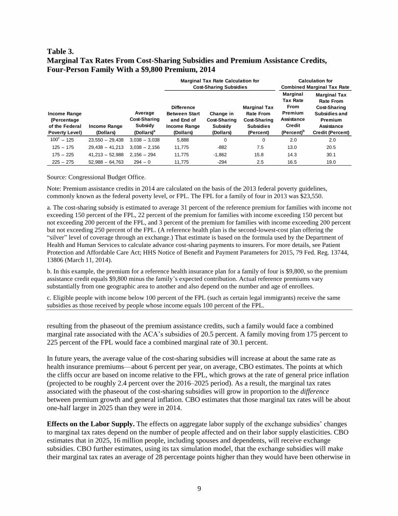
Table 3.
Marginal Tax Rates From Cost-Sharing Subsidies and Premium Assistance Credits,
Four-Person Family With a $9,800 Premium, 2014
Source: Congressional Budget Office.
Note: Premium assistance credits in 2014 are calculated on the basis of the 2013 federal poverty guidelines,
commonly known as the federal poverty level, or FPL. The FPL for a family of four in 2013 was $23,550.
a. The cost-sharing subsidy is estimated to average 31 percent of the reference premium for families with income not
exceeding 150 percent of the FPL, 22 percent of the premium for families with income exceeding 150 percent but
not exceeding 200 percent of the FPL, and 3 percent of the premium for families with income exceeding 200 percent
but not exceeding 250 percent of the FPL. (A reference health plan is the second-lowest-cost plan offering the
“silver” level of coverage through an exchange.) That estimate is based on the formula used by the Department of
Health and Human Services to calculate advance cost-sharing payments to insurers. For more details, see Patient
Protection and Affordable Care Act; HHS Notice of Benefit and Payment Parameters for 2015, 79 Fed. Reg. 13744,
13806 (March 11, 2014).
b. In this example, the premium for a reference health insurance plan for a family of four is $9,800, so the premium
assistance credit equals $9,800 minus the family’s expected contribution. Actual reference premiums vary
substantially from one geographic area to another and also depend on the number and age of enrollees.
c. Eligible people with income below 100 percent of the FPL (such as certain legal immigrants) receive the same
subsidies as those received by people whose income equals 100 percent of the FPL.
resulting from the phaseout of the premium assistance credits, such a family would face a combined
marginal rate associated with the ACA’s subsidies of 20.5 percent. A family moving from 175 percent to
225 percent of the FPL would face a combined marginal rate of 30.1 percent.
In future years, the average value of the cost-sharing subsidies will increase at about the same rate as
health insurance premiums—about 6 percent per year, on average, CBO estimates. The points at which
the cliffs occur are based on income relative to the FPL, which grows at the rate of general price inflation
(projected to be roughly 2.4 percent over the 2016–2025 period). As a result, the marginal tax rates
associated with the phaseout of the cost-sharing subsidies will grow in proportion to the difference
between premium growth and general inflation. CBO estimates that those marginal tax rates will be about
one-half larger in 2025 than they were in 2014.
Effects on the Labor Supply. The effects on aggregate labor supply of the exchange subsidies’ changes
to marginal tax rates depend on the number of people affected and on their labor supply elasticities. CBO
estimates that in 2025, 16 million people, including spouses and dependents, will receive exchange
subsidies. CBO further estimates, using its tax simulation model, that the exchange subsidies will make
their marginal tax rates an average of 28 percentage points higher than they would have been otherwise in
100c– 125 23,550 – 29,438 3,038 – 3,038 5,888 0 0 2.0 2.0
125 – 175 29,438 – 41,213 3,038 – 2,156 11,775 -882 7.5 13.0 20.5
175 – 225 41,213 – 52,988 2,156 – 294 11,775 -1,862 15.8 14.3 30.1
225 – 275 52,988 – 64,763 294 – 0 11,775 -294 2.5 16.5 19.0
Marginal Tax Rate Calculation for
Cost-Sharing Subsidies
Calculation for
Combined Marginal Tax Rate
Income Range
(Percentage
of the Federal
Poverty Level)
Income Range
(Dollars)
Average
Cost-Sharing
Subsidy
(Dollars)a
Marginal Tax
Rate From
Cost-Sharing
Subsidies and
Premium
Assistance
Credit (Percent)
Difference
Between Start
and End of
Income Range
(Dollars)
Change in
Cost-Sharing
Subsidy
(Dollars)
Marginal Tax
Rate From
Cost-Sharing
Subsidies
(Percent)
Marginal
Tax Rate
From
Premium
Assistance
Credit
(Percent)b
10
that year. Through the substitution effect, that increase in marginal rates will reduce the amount of labor
supplied by subsidy recipients. The exchange subsidies also boost recipients’ effective income, on
average, by reducing their out-of-pocket spending on health care or health insurance. The resulting
income effect, like the substitution effect, will reduce the amount of labor that recipients supply.12
After calculating those changes in marginal and average tax rates for each tax return in the tax simulation
model and applying the appropriate labor supply elasticities, which vary according to income, CBO
estimates that exchange subsidies will make the labor supply of subsidy recipients, measured as the total
value of their hours worked, 12 percent smaller in 2025 than it would have been otherwise. However, the
affected families will account for only 3 percent of total earnings, so that response translates into a
0.35 percent reduction in the aggregate labor supply, measured as total compensation.
CBO does not expect the exchange subsidies to have a significant effect on the labor supply of workers
who currently have income well above 400 percent of the FPL or who are offered employment-based
health insurance, because those workers are generally ineligible for subsidies. By contrast, some
researchers believe that the exchange subsidies will encourage many full-time workers with employment-
based health insurance to reduce their labor supply—for instance, by switching to a part-time job that
does not offer health insurance and thus gaining access to the subsidies. That would reduce the amount of
labor supplied by those workers.13
In that view, exchange subsidies effectively constitute a tax on labor
supply for a broad range of workers.
In CBO’s judgment, however, exchange subsidies operate primarily as an implicit tax on employment-
based insurance.14
That tax can be avoided in various ways other than reducing the number of hours that
one works. A full-time worker could switch to a different full-time job, one that does not offer health
insurance; a full-time worker could switch to two part-time jobs; or a worker’s current employer could
decide to stop offering insurance. Therefore, CBO estimates that the exchange subsidies will reduce the
labor supplied by only a limited segment of the population—mostly people who have no offer of
employment-based coverage and whose income is either below or near 400 percent of the FPL.
The approach just described—applying labor supply elasticities to changes in marginal and average tax
rates—does not fully capture the ACA’s effects on the labor market decisions of a particular group:
people who are unemployed for part of the year, who expect to be employed for the rest of the year in a
job that offers health insurance, and who therefore expect to become ineligible for exchange subsidies
when they return to work. For that group, the availability of exchange subsidies during unemployment
reduces the burden of unemployment, effectively raising the marginal tax rate on working an additional
month.15
CBO expects the exchange subsidies to lengthen the spells of unemployment for people in that
12 For an illustration of how the subsidies affect work incentives for a hypothetical family through the income and substitution
effects, see Congressional Budget Office, Answers to Questions for the Record Following a Hearing on the Budget and
Economic Outlook for 2014 to 2024 Conducted by the House Committee on the Budget (June 2014), pp. 9–10,
www.cbo.gov/publication/45318.
13 See Casey B. Mulligan, Average Marginal Labor Income Tax Rates Under the Affordable Care Act, Working Paper 19365
(National Bureau of Economic Research, August 2013), www.nber.org/papers/w19365, and Is the Affordable Care Act Different
From Romneycare? A Labor Economics Perspective, Working Paper 19366 (National Bureau of Economic Research, August
2013), www.nber.org/papers/w19366.
14 The consequences of that implicit tax are incorporated into CBO’s estimate of the ACA’s effect on employment-based
coverage—which is projected to decline because of the ACA, relative to what would have occurred otherwise.
15 That effect, which comes from the implicit taxes associated with working in a particular month, differs from the effect on
marginal tax rates described earlier in this paper, which was the effect on taxes of earning additional income at any point in the
year.
11
group, much as a comparable increase in the value of unemployment insurance benefits would. (That
effect will be muted, however, by the fact that exchange subsidies are based on annual rather than
monthly income; people who become employed and see their income rise may have to pay back some of
their subsidies through their end-of-the-year tax filings.)
That group will consist of about 4 million families in 2025, CBO estimates. That is, roughly 4 million
families will have annual income between 100 percent and 400 percent of the FPL, work less than a full
year, and be covered by employer-sponsored health insurance during the months when they work. Those
families will account for just under 2 percent of economywide earnings. For that group, CBO calculated
the change in the marginal rate on working an additional month as the value of one month’s exchange
subsidies divided by one month’s earnings, adjusted for the probability of participating in the health
insurance exchanges. The result was an increase in the marginal tax rate of about 16 percentage points for
the group. That change in the marginal rate, when multiplied by the relevant substitution elasticity (an
average of 0.25 for the group), implies a 4 percent reduction in the labor supply for the group—the
equivalent of about two weeks of work, on average. That 4 percent reduction multiplied by the group’s
2 percent share of economywide earnings equals a 0.08 percent reduction in the aggregate supply of labor.
Combining that effect with the other effects of exchange subsidies described above yields an estimated
reduction in the labor supply of 0.43 percent in 2025.
Rules Governing Insurance
Changes that the ACA has made to the individual (or nongroup) health insurance market—including
provisions that prohibit insurers from denying coverage to people with preexisting health conditions and
provisions that restrict variation in premiums on the basis of age—lower the cost of insurance plans
available to many older people outside the workplace. As a result, some will choose to retire earlier than
they would have otherwise, CBO expects.
To estimate the ACA’s effects on the labor supplied by workers near retirement, CBO studied the effects
of analogous policies—specifically, policies that require employers to keep offering workers insurance
coverage after they have left a job. Those policies, such as the ones established by the Consolidated
Omnibus Budget Reconciliation Act (COBRA) and similar state mandates, allow employees to buy health
insurance coverage from their employer for a certain number of months after leaving, and those
employees may be charged only slightly more than the average premium for that coverage at the entire
firm. Because older workers tend to have above-average health care costs, that average premium is
generally less than the cost of an individually purchased plan with a comparable level of coverage. Such
policies therefore reduce the cost of purchasing health insurance in retirement and make retirement more
attractive, much as the ACA’s provisions do.
One study examining the effects of enacting COBRA and similar mandates found that among workers
with employment-based insurance who were between the ages of 55 and 64, the probability of retirement
increased by 2.25 percent.16
In CBO’s view, the response caused by the ACA will be similar, so the
agency estimates that in 2025, of the estimated 10 million workers who will have employment-based
insurance and be between the ages of 55 and 64, 2.25 percent—or 225,000 workers—will retire earlier
than they would have otherwise. CBO estimates that the total labor force will consist of almost
170 million people in 2025, so those early retirements will reduce that number by about 0.1 percent.
Because older workers’ earnings are much higher than average, that effect translates into a larger
reduction—of 0.17 percent—in total compensation.
16 Jonathan Gruber and Brigitte C. Madrian, “Health-Insurance Availability and the Retirement Decision,” American Economic
Review, vol. 85, no. 4 (September 1995), pp. 938–948, www.jstor.org/stable/2118241.
12
Medicaid Expansion
The ACA also subsidizes health insurance by making many more people eligible for Medicaid—a
program that usually does not charge premiums and covers essentially all of the costs of enrollees’ care
for a comprehensive set of benefits. Before the ACA was enacted, eligibility varied considerably by state
but was generally limited to low-income children, parents, and pregnant women, as well as certain
disabled people with low income and low assets.17
Now, in states that choose to expand their Medicaid
programs under the ACA, eligibility is extended to most nonelderly residents—including childless
adults—whose modified adjusted gross income is below 138 percent of the FPL. By 2020, CBO
estimates, about 80 percent of the people in the country who could be eligible under the new criteria will
live in states that have expanded Medicaid, and the same percentage is projected for 2025.
By 2025, CBO estimates that the Medicaid expansion will decrease the labor supply (measured as total
compensation) by 0.05 percent. The relatively small size of that effect results from a number of factors.
For one thing, the expansion has offsetting effects, decreasing work incentives for some people and
increasing them for others. For another, the affected workers will have relatively low wages.
To analyze the expansion’s effects on the labor supply, CBO focused on three groups: newly eligible
enrollees (that is, low-income adults who would not have been eligible for Medicaid in the absence of the
ACA); low-income adults who were already eligible under prior law; and certain workers, particularly
secondary earners, with income somewhat higher than Medicaid’s new eligibility threshold.
Newly Eligible Enrollees. Most of the increase in Medicaid enrollment stemming from the ACA consists
of people who would not have been eligible for Medicaid in the absence of that law. Enrolling in
Medicaid reduces their out-of-pocket spending on health care, thus boosting their ability to consume and
reducing their incentive to work via the income effect.18
Also, they would lose eligibility if their income
rose above 138 percent of the FPL, which effectively creates a tax on additional earnings for those
considering job changes that would push them above that point: Although they could receive premium
assistance credits and cost-sharing subsidies through the exchanges, they would no longer get free care.
That implicit tax reduces the incentive to work via the income and substitution effects. In addition, the
Medicaid expansion allows some people to switch from employer-sponsored health insurance to Medicaid
and then to reduce their supply of labor—since they can reduce the number of hours that they work and
retain health insurance.
Of the people who will be newly eligible enrollees in 2025, CBO estimates that 4.8 million—about
3 percent of the labor force, accounting for less than 1 percent of economywide earnings—would have
been working in the absence of the ACA. CBO further estimates that the Medicaid expansion will reduce
their labor force participation by almost 4 percent. The agency based that estimate on studies that
examined previous changes in eligibility for public health insurance coverage.19
CBO estimates that their
17 For details about income limits for various eligibility groups, see Tricia Brooks and others, Modern Era Medicaid: Findings
From a 50-State Survey of Eligibility, Enrollment, Renewal, and Cost-Sharing Policies in Medicaid and CHIP as of January
2015 (Kaiser Commission on Medicaid and the Uninsured, January 2015), http://tinyurl.com/nav6ga6.
18 The size of the income change for those enrollees is a subject of some debate. However, because CBO relied on studies of
state-level changes in Medicaid eligibility to estimate the effects of the expansion on work incentives, the agency did not have to
estimate a specific value for the income change.
19 See Katherine Baicker and others, “The Impact of Medicaid on Labor Market Activity and Program Participation: Evidence
from the Oregon Health Insurance Experiment,” American Economic Review, vol. 104, no. 5 (May 2014), pp. 322–328,
http://dx.doi.org/10.1257/aer.104.5.322; Laura Dague, Thomas DeLeire, and Lindsey Leininger, The Effect of Public Insurance
Coverage for Childless Adults on Labor Supply, Working Paper 20111 (National Bureau of Economic Research, May 2014),
www.nber.org/papers/w20111; Craig Garthwaite, Tal Gross, and Matthew J. Notowidigdo, “Public Health Insurance, Labor
Supply, and Employment Lock,” Quarterly Journal of Economics, vol. 129, no. 2 (2014), pp. 653–696,
13
response will translate into a 0.03 percent reduction in the labor supply, measured as total compensation
(a 4 percent reduction for affected employees multiplied by their share of economywide earnings, which
is less than 1 percent).
Previously Eligible Enrollees. People who would already have been eligible for Medicaid under prior
law will see their work incentives affected by the higher income limits for Medicaid and by the
availability of exchange subsidies.20
Most of those people would have enrolled in Medicaid in the absence
of the ACA, and their work incentives will increase.21
In particular, if their income exceeds the income
limit for Medicaid, they will still lose eligibility for the program, as they would have before the ACA was
enacted—but that incentive not to earn more is now smaller if they live in a state that has expanded
Medicaid under the ACA, because the income limit is higher. Further, even if they do exceed the limit,
they may now be able to receive exchange subsidies.22
The conclusion that the ACA will increase the work incentives of previously eligible enrollees is
supported by various studies of the effect of state-level increases in income limits for Medicaid eligibility.
Those studies have found convincing evidence that such increases encourage nonworkers to work, but
only weak evidence that they encourage workers to limit their earnings to stay below the income limit.23
CBO estimates that of the 4.9 million nonworkers who will be enrolled in Medicaid in 2025 but who
would have been eligible for and enrolled in the program under pre-ACA rules, 2 percent (or about
100,000) will join the labor force because of the ACA. The agency estimates that those responses will
increase the labor supply (measured as total compensation) by 0.01 percent.
Workers With Income Somewhat Higher Than the New Eligibility Threshold. The ACA is also
expected to reduce the work incentives of some people whose income will be slightly higher than the new
eligibility threshold of 138 percent of the FPL. In states that will have expanded their programs, such
people could become eligible for Medicaid if they reduced their earnings so that their family income
dropped below the new threshold for eligibility.24
They would be more likely to do so if they were
http://tinyurl.com/pvxdt34; and Vincent Pohl, Medicaid and the Labor Supply of Single Mothers: Implications for Health Care
Reform, Working Paper 15-222 (Upjohn Institute for Employment Research, May 2014), http://tinyurl.com/o2dkumq. For a
review of those studies, see Bowen Garrett and Robert Kaestner, The Best Evidence Suggests the Effects of the ACA on
Employment Will Be Small (Urban Institute, April 2014), http://tinyurl.com/olasnp6.
20 Because the effects of the Medicaid expansion are intertwined with those of the exchange subsidies, allocating the changes in
work incentives to one provision or the other is difficult—but different allocations do not alter CBO’s overall estimate of the
change in work incentives.
21 However, CBO’s estimate of the total effect on the labor supply also includes a small effect from people who would not have
been enrolled under prior law and who were induced to enroll by the ACA. That group faces a more ambiguous set of incentives.
On balance, CBO expects them to reduce their supply of labor—because they will receive new benefits that are gradually phased
out, just as newly eligible enrollees will.
22 In states where the income limit for Medicaid eligibility remains below the FPL, enrollees still risk losing eligibility for
subsidized health insurance if their income rises above the level of Medicaid eligibility but stays below the FPL. At the same
time, the availability of exchange subsidies will increase work incentives for people in those states who are currently ineligible
for Medicaid and whose income is below the FPL. Such people have a new incentive to increase their income to the FPL in order
to qualify for exchange subsidies. However, CBO has not estimated the resulting effect on the labor supply.
23 See John C. Ham and Lara D. Shore-Sheppard, “Did Expanding Medicaid Affect Welfare Participation?” ILR Review, vol. 58,
no. 3 (April 2005), pp. 452–470, http://tinyurl.com/nbobszm; Sarah Hamersma, “The Effects of Medicaid Earnings Limits on
Earnings Growth Among Poor Workers,” The B.E. Journal of Economic Analysis & Policy, vol. 13, no. 2 (August 2013),
pp. 887–919, http://tinyurl.com/nu4fars; and Vincent Pohl, Medicaid and the Labor Supply of Single Mothers: Implications for
Health Care Reform, Working Paper 15-222 (Upjohn Institute for Employment Research, May 2014), http://tinyurl.com/
o2dkumq.
24 Some workers faced that incentive under prior law as well, especially in states with higher eligibility thresholds for Medicaid.
However, the thresholds for parents in many states were well below 138 percent of the FPL, and childless adults were generally
14
ineligible for exchange subsidies, so CBO expects that most of them would be secondary workers who
had employment-based health insurance and were therefore barred from getting such subsidies.
CBO estimates that among the 1.4 million secondary workers who will have employment-based coverage
and a family income between 138 percent and 250 percent of the FPL in 2025, the Medicaid changes will
reduce labor force participation by 15 percent. The effect will reduce the labor supply (measured as total
compensation) by 0.03 percent, CBO estimates.
Effects of Taxes and Penalties
This section of the paper describes the second group of ACA provisions that affect the labor supply—
those that impose taxes and penalties on employers or on labor income. The ACA levies several such
taxes and penalties: a surtax on earnings above a certain level that is credited to Medicare’s HI program;
penalties on larger employers that do not offer qualifying health insurance coverage to their employees;
an excise tax on high-premium health insurance plans offered through employers; and penalties on certain
individuals who are uninsured. Although some of those taxes and penalties are initially levied on
employers and insurers, CBO expects their costs to be passed on to workers in ways that affect their
incentives to work. The agency estimates that together, the taxes and penalties will reduce the supply of
labor, measured as the total compensation paid to workers, by 0.21 percent in 2025 (see Table 1 on
page 2).
Hospital Insurance Surtax
The ACA raises the Medicare payroll tax by 0.9 percentage points for workers who earn more than
$200,000 per year (or $250,000 for those filing a joint return).25
Those thresholds are not adjusted for
inflation, so over time, the surtax will apply to a growing share of workers and a growing share of their
earnings.
CBO estimates that roughly 8 percent of workers will be subject to the surtax in 2025 and that those
workers will have 38 percent of the economy’s total earnings. On average, the surtax will raise their
marginal tax rate from roughly 44 percent to 45 percent, which is about a 1.8 percent decrease in their
net-of-tax marginal rate [(100 − 45) ÷ (100 − 44) − 1]. CBO estimates that those workers’ earnings will
consequently fall by 0.39 percent (1.8 percent multiplied by the substitution elasticity for high-income
earners, which averages 0.22). That translates into a 0.15 percent reduction in the economy’s total labor
supply, measured as total compensation (0.39 percent times 38 percent). That effect will be slightly offset
by an income effect, calculated by means of a similar procedure. On net, the surtax will reduce the labor
supply by 0.12 percent, CBO estimates.
Employer Mandate and Penalty
The ACA generally imposes a penalty on employers if they have 50 or more full-time-equivalent
employees and do not offer insurance that meets certain standards. In CBO’s view, after a few years, the
costs of the penalty will be passed on to workers in the form of reduced wages (just as payroll taxes levied
not eligible at all. Because the ACA extends eligibility to most nonelderly people whose income is below 138 percent of the
FPL—whether or not they have children—more adults face the incentive now than in the past.
25 The ACA also raises the tax rate on capital income for some higher-income households. CBO does not expect that provision to
have a noticeable effect on the overall labor market—but it will affect savings and investment, so it is incorporated into the
agency’s estimate of the ACA’s effects on GDP.
15
on employers are). Therefore, the agency models the penalty as a payroll tax, affecting the supply of but
not the demand for labor.26
The employer penalty took effect in 2015, will equal $2,160 per full-time worker in 2016, and will apply
to each full-time worker after the first 30, starting in 2016; the amount of the penalty for future years is
indexed to the average growth of health insurance premiums.27
By 2025, CBO expects that the amount
will be about $3,500. However, employers will have to reduce wages by a larger amount than that. If they
reduced wages by only a sum equal to the amount of the penalty payments, their accounting profits would
rise, because the ACA prohibits them from deducting the penalty as an expense; they would therefore
have to pay business taxes on the higher accounting profits. To compensate for the additional taxes,
employers will reduce wages by more than the amount of the penalty payments.
CBO calculates the penalty’s change in the marginal rate on the extensive margin, rather than on the
intensive margin—because, in the agency’s view, the penalty reduces a worker’s return on accepting a
full-time job but generally does not affect a worker’s return on working another hour. CBO estimates that
the penalty will represent a 7 percent increase in the tax rate of workers at firms that are potentially
subject to the penalty. As a result, CBO estimates, the penalty will reduce the labor supplied by those
workers by about 1.3 percent. Because those workers account for only about 5 percent of earnings in the
economy, the estimated effect on the entire labor supply is considerably smaller: 0.06 percent of total
compensation.
The employer penalty also creates incentives for some businesses to reduce their hiring or to shift their
workforce toward part-time jobs—either to stay below the threshold of 50 full-time-equivalent workers or
to limit the number of full-time workers who generate penalty payments. Those shifts in the composition
of employment could reduce productivity if part-time workers operated less efficiently than full-time
workers did. Such reductions in productivity are difficult to quantify, but they would probably be small,
so they are not incorporated into CBO’s estimates of the effects of the ACA on the labor market.28
High-Premium Excise Tax
Beginning in 2018, the ACA will impose a 40 percent excise tax on certain employment-based health
insurance plans with high premiums. In 2018, the tax will apply to premiums for single coverage that are
higher than $10,200 per year and to premiums for family coverage that are higher than $27,500 per year.
CBO and JCT estimate that roughly one out of every 10 people enrolled in an employment-based health
insurance plan in 2018 will be affected by the excise tax and that most will avoid the excise tax through
changes to their health coverage. The thresholds are generally scheduled to increase at the rate of
inflation. Because premiums are projected to grow more quickly than inflation, an increasing share of
plans will be affected by the excise tax over time.
26 In the short term, however, the penalty may be borne by employers, either because wages are not adjusted quickly or because
minimum-wage laws constrain employers’ ability to reduce wages. That outcome would lead employers to reduce their demand
for labor.
27 A separate penalty applies to firms that offer coverage that does not qualify as affordable under federal rules; that penalty,
which is not expected to have significant effects on the labor supply because it will apply much less often, is discussed further in
Congressional Budget Office, The Budget and Economic Outlook: 2014 to 2024 (February 2014), Appendix C,
www.cbo.gov/publication/45010.
28 The ACA could also increase productivity—for example, if increases in insurance coverage stemming from the ACA improved
workers’ health. Such increases in productivity are not incorporated into CBO’s estimates either. For more discussion about the
ACA’s potential effects on workers’ productivity, see Congressional Budget Office, Budgetary and Economic Effects of
Repealing the Affordable Care Act (June 2015), pp. 18–19, www.cbo.gov/publication/50252.
16
Although the tax will sometimes be levied on insurers rather than employers, CBO expects those insurers
to pass the cost on to employers in the form of higher premiums. Like the employer penalty, the tax is not
a deductible expense, so insurers will have to raise premiums by more than the amount of the tax (and
employers subject to the tax will be affected similarly). In any event, CBO expects the tax ultimately to be
passed on from the employers to their workers.
The excise tax will raise average tax rates, CBO estimates, slightly increasing the supply of labor through
the income effect. Average tax rates will rise even though many firms may avoid the excise tax by
switching to less expensive health plans. In that case, CBO estimates, workers’ wages would rise by a
corresponding amount in order to hold total compensation about the same—but those wages would be
subject to income and payroll taxes, so the workers’ total tax payments would be greater than they would
have been in the absence of the ACA. Those higher taxes, combined with the less expensive health plans
that the workers received, would mean that their total after-tax compensation was lower and therefore that
their average tax rates were higher.
CBO also believes that the excise tax will raise the marginal tax rate on labor slightly, causing the labor
supply to fall through the substitution effect. That increase in marginal rates will occur because people are
projected to use some of the income that they gain from any additional work to purchase health insurance.
Before the ACA was enacted, those purchases would not have been taxed. But under the ACA, workers
with high-premium plans will have to pay the excise tax on those purchases—or else forgo such
purchases and receive their additional income in the form of taxable wages; the marginal tax rate on their
labor will rise in either case.29
To estimate the effect of the excise tax on marginal tax rates that apply to labor compensation, CBO first
estimated that the costs of employment-based health insurance would equal about 8 percent of labor
compensation over the 2016–2025 period. CBO uses an income elasticity of 0.15 for health insurance
spending, which implies that, on average, only 1.2 cents of each additional dollar earned would be spent
on health insurance. Only a portion of that 1.2 cents would be subject to the excise tax, however, because
a significant share of plans will remain under the excise tax threshold, even by 2025. On net, CBO
estimates that the excise tax will raise the marginal tax rate on labor income by roughly 0.1 percentage
point in 2025.
That effect of the increase in marginal tax rates on the labor supply (through the substitution effect) will
more than offset the effect of the increase in average rates (through the income effect). On balance, the
estimated result is a 0.03 percent reduction in the labor supply in 2025.
Individual Mandate and Penalty
The ACA also imposes a penalty on many people who do not have qualifying health insurance. In 2016,
the penalty will be the greater of two numbers: $695 per person in a household or 2.5 percent of
household income in excess of the general tax-filing threshold (both of which are subject to specified
caps).
The percentage-of-income version of the penalty represents an increase in the marginal tax rate of
2.5 percent. That increase would tend to reduce the labor supplied by people who pay that version of the
29 Insurance is usually offered in a fixed amount by employers, so in the near term, workers often have little flexibility to change
the amount that they spend on health insurance. Over time, however, as their income rises, employees have tended to seek more
expensive health insurance plans from their employers (which is one reason that premiums for those plans have risen over time).
That connection in the longer run between changes in income and desired increases in health insurance spending underlies CBO’s
conclusion that the excise tax will raise effective marginal tax rates on labor.
17
penalty through the substitution effect. In contrast, the fixed-dollar version of the penalty has essentially
no effect on marginal tax rates.
CBO’s analysis of the individual mandate’s effects on the labor supply is based on a previous analysis of
the population expected to be uninsured in 2016.30
In that year, by CBO and JCT’s estimates, about
30 million people will be uninsured, but most of them will be eligible for various exemptions from the
penalty—for example, because their income is below the tax-filing threshold. Some of the remainder will
be subject to the penalty but will try to avoid such payments, and in the end, only about 4 million people
will pay the penalty, the agencies estimated.
Of those 4 million people, about half will pay the percentage-of-income version. For those 2 million or so
people, the penalty will increase the marginal tax rate from roughly 30 percent to 32.5 percent, which is
about a 3.6 percent decrease in the net-of-tax marginal rate [(100 − 32.5) ÷ (100 − 30) − 1]. CBO
estimates that as a result, those workers’ pretax earnings will fall by 0.9 percent—that is, 3.6 percent
multiplied by the substitution elasticity, which averages about 0.25 for affected earners. CBO estimates
that the affected workers account for less than 1 percent of earnings in the economy. Consequently, the
agency estimates that the substitution effect stemming from the individual mandate will reduce the total
labor supply by only 0.01 percent in 2016. In years after 2016, CBO estimates that a similar percentage of
the uninsured population will be subject to the percentage-of-income version of the penalty, so the
reduction in 2025 is likewise estimated to be 0.01 percent.
Both versions of the penalty also reduce after-tax income, causing a small increase in the labor supply
through the income effect. However, that increase only slightly offsets the reduction in the labor supply
caused by the percentage-of-income version of the penalty, so the net effect of the individual mandate
remains a 0.01 percent reduction.
Effects on Total Hours and Full-Time-Equivalent Employment
In general, CBO estimated the ACA’s effects on the labor supply in terms of total compensation, because
that calculation can be translated most directly into the law’s effect on GDP—which, in turn, affects the
agency’s budgetary projections. In general, CBO did not calculate how much of that total effect on the
labor supply would consist of changes in labor force participation and how much would consist of
changes in the number of hours worked by those in the labor force; the reason is that the agency’s labor
supply elasticities combine these two decisions.31
CBO did, however, translate the effect on the labor
supply into effects on full-time-equivalent employment and on total hours worked.
To find the effect on full-time-equivalent employment, CBO began with its estimate that implementing
the ACA would reduce the supply of labor, measured as total compensation, by 0.86 percent, or
$120 billion, in 2025. CBO divided that number by roughly $61,000, the estimated annual earnings of
full-time-equivalent workers affected by the ACA (that is, what workers affected by the ACA would earn
30 Congressional Budget Office, Payments of Penalties for Being Uninsured Under the Affordable Care Act: 2014 Update (June
2014), www.cbo.gov/publication/45397.
31 Two exceptions are CBO’s estimates of the effects of the Medicaid expansion on the labor supply and the effects of the
exchange subsidies on the labor supplied by people close to retirement. In those cases, to calculate the effects on earnings, the
agency estimated the number of people who would drop out of the labor force and then multiplied those amounts by estimates of
the average earnings of the workers affected by the changes.
18
if they worked full time for all of 2025).32
The result was an estimated reduction in full-time-equivalent
workers of about 2 million.
To estimate the ACA’s effect on total hours worked, CBO divided that reduction in full-time-equivalent
employment by the agency’s projection of full-time-equivalent employment in the entire economy in
2025—about 138 million full-time-equivalent workers. The result was an estimated 1.7 percent decrease
in total hours worked. The finding that the percentage decline in terms of hours worked is almost twice as
large as the percentage decline in terms of earnings reflects CBO’s assessment that the average earnings
of workers who will work less as a result of the ACA’s provisions will be about half of the national
average.
Uncertainty of the Effects
CBO’s estimates of the ACA’s effects on the labor supply are uncertain, because they are based on
various factors that are themselves uncertain. Above all, they are based in large part on CBO’s projections
of the law’s effects on health insurance coverage and on the federal budget, which are highly uncertain
and could deviate in either direction from the agency’s estimates. For example, if fewer people receive
exchange subsidies than CBO expects, the ACA’s effects on employment will be smaller than estimated
in this paper, and vice versa.
Another uncertain factor is the magnitude of people’s responses to the work incentives created by the
ACA. Not only does a range of estimates exist regarding how labor supply responds to general tax
changes; there is additional uncertainty about whether people will respond to the ACA’s provisions in the
same way that they respond to general tax changes. For instance, if people do not readily perceive that the
exchange subsidies effectively change their marginal tax rates—because of the complexity of the
calculation or of the linkages between purchasing insurance and receiving a subsidy—they might be less
responsive to the subsidies than to more readily visible taxes.
For this analysis, CBO did not quantify the uncertainty related to the ACA’s effects on insurance
coverage and the budget. Many other sources of uncertainty surrounding the ACA’s effects on labor
supply could likewise not be quantified.
However, CBO did quantify the uncertainty related to people’s responses to work incentives. In cases
when CBO’s central estimate of the labor supply effect was based on the law’s effects on marginal and
average tax rates, the agency used a range of estimates of how responsive people might be to the changes
in incentives created by the law—that is, using a lower estimate and a higher estimate for elasticities in
addition to the central estimates presented above. The agency drew the range of elasticities from a review
of studies of people’s responses to general changes in tax rates and income; each range is intended to
cover roughly the middle two-thirds of the likely values for the elasticity.33
Specifically, CBO’s range of
likely labor supply responses for all earners taken together is bounded at the low end by a substitution
elasticity of 0.16 and at the high end by an elasticity of 0.32 (see Table 4). CBO’s central estimate
32 Workers affected by the ACA are projected to have annual earnings averaging $46,000 in 2025, but many of them would not
work full time for the full year (that is, 2,080 hours over the course of the year). CBO converted their annual earnings into full-
time-equivalent annual earnings by assuming that they would work, on average, the same number of hours that workers in the
population as a whole would work: roughly 1,560. Thus the affected workers’ full-time-equivalent earnings were calculated as
$46,000 × (2,080 ÷ 1,560).
33 For more details, see Congressional Budget Office, How the Supply of Labor Responds to Changes in Fiscal Policy (October
2012), www.cbo.gov/publication/43674; and Robert McClelland and Shannon Mok, A Review of Recent Research on Labor
Supply Elasticities, Working Paper 2012-12 (Congressional Budget Office, October 2012), www.cbo.gov/publication/43675.
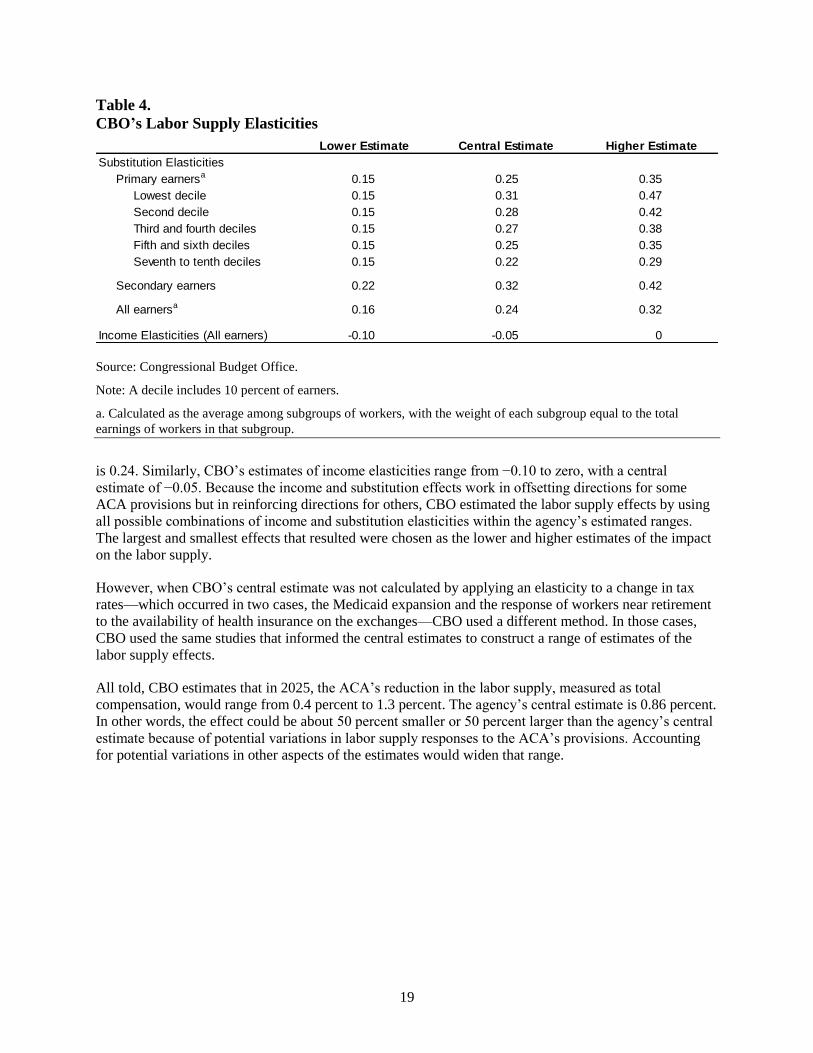
19
Table 4.
CBO’s Labor Supply Elasticities
Source: Congressional Budget Office.
Note: A decile includes 10 percent of earners.
a. Calculated as the average among subgroups of workers, with the weight of each subgroup equal to the total
earnings of workers in that subgroup.
is 0.24. Similarly, CBO’s estimates of income elasticities range from −0.10 to zero, with a central
estimate of −0.05. Because the income and substitution effects work in offsetting directions for some
ACA provisions but in reinforcing directions for others, CBO estimated the labor supply effects by using
all possible combinations of income and substitution elasticities within the agency’s estimated ranges.
The largest and smallest effects that resulted were chosen as the lower and higher estimates of the impact
on the labor supply.
However, when CBO’s central estimate was not calculated by applying an elasticity to a change in tax
rates—which occurred in two cases, the Medicaid expansion and the response of workers near retirement
to the availability of health insurance on the exchanges—CBO used a different method. In those cases,
CBO used the same studies that informed the central estimates to construct a range of estimates of the
labor supply effects.
All told, CBO estimates that in 2025, the ACA’s reduction in the labor supply, measured as total
compensation, would range from 0.4 percent to 1.3 percent. The agency’s central estimate is 0.86 percent.
In other words, the effect could be about 50 percent smaller or 50 percent larger than the agency’s central
estimate because of potential variations in labor supply responses to the ACA’s provisions. Accounting
for potential variations in other aspects of the estimates would widen that range.
Substitution Elasticities
Primary earnersa 0.15 0.25 0.35
Lowest decile 0.15 0.31 0.47
Second decile 0.15 0.28 0.42
Third and fourth deciles 0.15 0.27 0.38
Fifth and sixth deciles 0.15 0.25 0.35
Seventh to tenth deciles 0.15 0.22 0.29
Secondary earners 0.22 0.32 0.42
All earnersa 0.16 0.24 0.32
Income Elasticities (All earners) -0.10 -0.05 0
Lower Estimate Central Estimate Higher Estimate