catia v5 fea tutorials

CATIA V5

FEA Tutorials Releases 12 & 13

Nader G. Zamani University of Windsor

SDC

Schroff Development Corporation

www.schroff.com

www.schroff-europe.com

PUBLICATIONS

Visit our website to learn more about this and other books:

http://www.sdcpublications.com/

Copyrighted Material

Copyrighted

Material


Copyrighted

Material

CATIA V5 FEA Tutorials 2-1

Chapter 2

Analysis of a Bent Rod with

Solid Elements


Copyrighted

Material


Copyrighted

Material

2-2 CATIA V5 FEA Tutorials

Clamped end

loaded end

Clamped end

loaded end

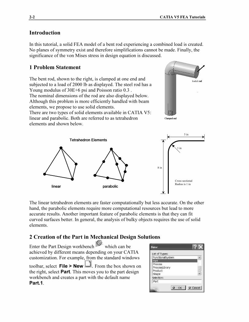
Introduction

In this tutorial, a solid FEA model of a bent rod experiencing a combined load is created.

No planes of symmetry exist and therefore simplifications cannot be made. Finally, the

significance of the von Mises stress in design equation is discussed.

1 Problem Statement

The bent rod, shown to the right, is clamped at one end and

subjected to a load of 2000 lb as displayed. The steel rod has a

Young modulus of 30E+6 psi and Poisson ratio 0.3 .

The nominal dimensions of the rod are also displayed below.

Although this problem is more efficiently handled with beam

elements, we propose to use solid elements.

There are two types of solid elements available in CATIA V5:

linear and parabolic. Both are referred to as tetrahedron

elements and shown below.

The linear tetrahedron elements are faster computationally but less accurate. On the other

hand, the parabolic elements require more computational resources but lead to more

accurate results. Another important feature of parabolic elements is that they can fit

curved surfaces better. In general, the analysis of bulky objects requires the use of solid

elements.

2 Creation of the Part in Mechanical Design Solutions

Enter the Part Design workbench which can be

achieved by different means depending on your CATIA

customization. For example, from the standard windows

toolbar, select File > New . From the box shown on

the right, select Part. This moves you to the part design

workbench and creates a part with the default name

Part.1.

5 in

8 in

1 in

Cross sectional

Radius is 1 in

Tetrahedron Elements

linear parabolic

Tetrahedron Elements

linear parabolic


Copyrighted

Material


Copyrighted

Material

Analysis of a Bent Rod with Solid Elements 2-3

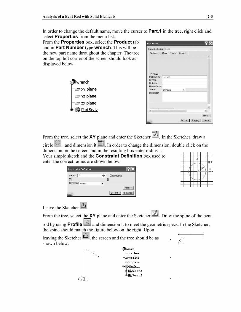
In order to change the default name, move the curser to Part.1 in the tree, right click and

select Properties from the menu list.

From the Properties box, select the Product tab

and in Part Number type wrench. This will be

the new part name throughout the chapter. The tree

on the top left corner of the screen should look as

displayed below.

From the tree, select the XY plane and enter the Sketcher . In the Sketcher, draw a

circle , and dimension it . In order to change the dimension, double click on the

dimension on the screen and in the resulting box enter radius 1.

Your simple sketch and the Constraint Definition box used to

enter the correct radius are shown below.

Leave the Sketcher .

From the tree, select the XY plane and enter the Sketcher . Draw the spine of the bent

rod by using Profile and dimension it to meet the geometric specs. In the Sketcher,

the spine should match the figure below on the right. Upon

leaving the Sketcher , the screen and the tree should be as

shown below.


Copyrighted

Material


Copyrighted

Material


You will now use the ribbing operation to extrude the

circle along the spine (path). Upon selecting the rib

icon , the Rib Definition box opens. Select the

circle (Sketch.1) and the spine (Sketch.2) as

indicated. The result is the final part shown below.

Regularly save your work.

3 Entering the Analysis Solutions

From the standard windows tool bar, select

Start > Analysis & Simulation > Generative Structural Analysis

There is a second workbench known as the Advanced Meshing Tools which will be

discussed later.

The first thing one can note is the presence of a

“Warning” box indicating that material is not

properly defined on wrench. This is not

surprising since material has not yet been

assigned. This will be done shortly and

therefore you can close this box by pressing

“OK”.

A second box shown below, “New Analysis

Case” is also visible. The default choice is

“Static Analysis” which is precisely what we

intend to use. Therefore, close the box by

clicking on “OK”.


Copyrighted

Material


Copyrighted

Material


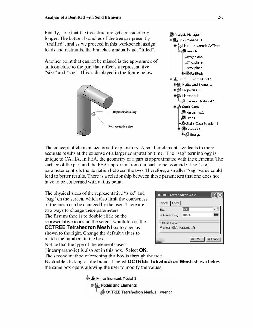
Finally, note that the tree structure gets considerably

longer. The bottom branches of the tree are presently

“unfilled”, and as we proceed in this workbench, assign

loads and restraints, the branches gradually get “filled”.

Another point that cannot be missed is the appearance of

an icon close to the part that reflects a representative

“size” and “sag”. This is displayed in the figure below.

The concept of element size is self-explanatory. A smaller element size leads to more

accurate results at the expense of a larger computation time. The “sag” terminology is

unique to CATIA. In FEA, the geometry of a part is approximated with the elements. The

surface of the part and the FEA approximation of a part do not coincide. The “sag”

parameter controls the deviation between the two. Therefore, a smaller “sag” value could

lead to better results. There is a relationship between these parameters that one does not

have to be concerned with at this point.

The physical sizes of the representative “size” and

“sag” on the screen, which also limit the coarseness

of the mesh can be changed by the user. There are

two ways to change these parameters:

The first method is to double click on the

representative icons on the screen which forces the

OCTREE Tetrahedron Mesh box to open as

shown to the right. Change the default values to

match the numbers in the box.

Notice that the type of the elements used

(linear/parabolic) is also set in this box. Select OK.

The second method of reaching this box is through the tree.

By double clicking on the branch labeled OCTREE Tetrahedron Mesh shown below,

the same box opens allowing the user to modify the values.

Representative sag

Representative size

Representative sag

Representative size


Copyrighted

Material


Copyrighted

Material


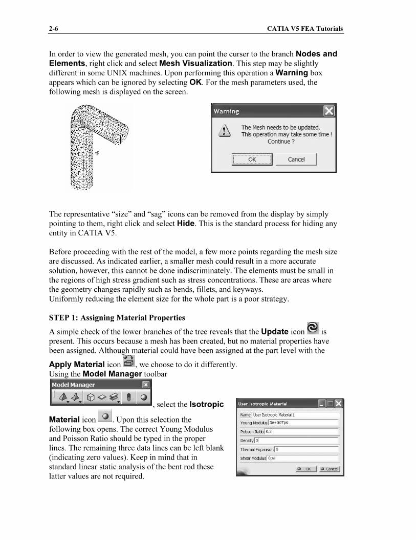
In order to view the generated mesh, you can point the curser to the branch Nodes and Elements, right click and select Mesh Visualization. This step may be slightly

different in some UNIX machines. Upon performing this operation a Warning box

appears which can be ignored by selecting OK. For the mesh parameters used, the

following mesh is displayed on the screen.

The representative “size” and “sag” icons can be removed from the display by simply

pointing to them, right click and select Hide. This is the standard process for hiding any

entity in CATIA V5.

Before proceeding with the rest of the model, a few more points regarding the mesh size

are discussed. As indicated earlier, a smaller mesh could result in a more accurate

solution, however, this cannot be done indiscriminately. The elements must be small in

the regions of high stress gradient such as stress concentrations. These are areas where

the geometry changes rapidly such as bends, fillets, and keyways.

Uniformly reducing the element size for the whole part is a poor strategy.

STEP 1: Assigning Material Properties

A simple check of the lower branches of the tree reveals that the Update icon is

present. This occurs because a mesh has been created, but no material properties have

been assigned. Although material could have been assigned at the part level with the

Apply Material icon , we choose to do it differently.

Using the Model Manager toolbar

, select the Isotropic

Material icon . Upon this selection the

following box opens. The correct Young Modulus

and Poisson Ratio should be typed in the proper

lines. The remaining three data lines can be left blank

(indicating zero values). Keep in mind that in

standard linear static analysis of the bent rod these

latter values are not required.


Copyrighted

Material


Copyrighted

Material


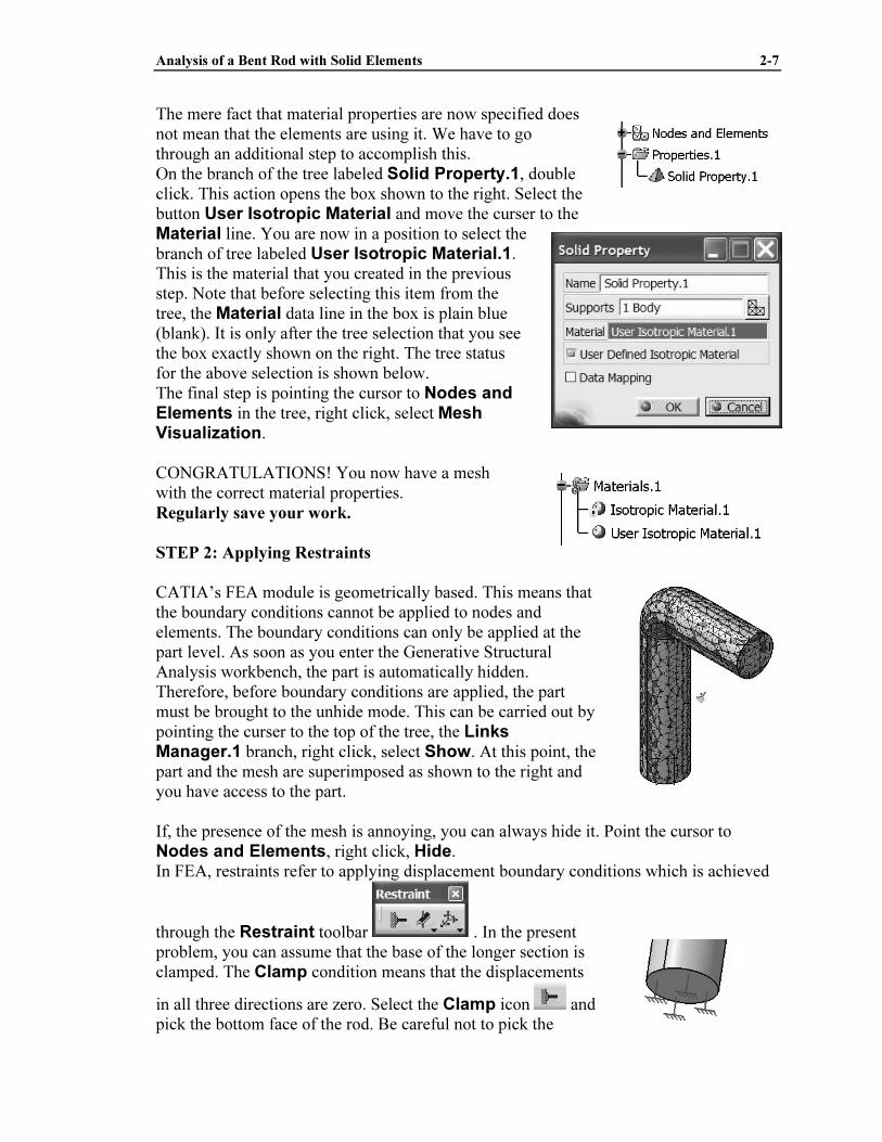
The mere fact that material properties are now specified does

not mean that the elements are using it. We have to go

through an additional step to accomplish this.

On the branch of the tree labeled Solid Property.1, double

click. This action opens the box shown to the right. Select the

button User Isotropic Material and move the curser to the

Material line. You are now in a position to select the

branch of tree labeled User Isotropic Material.1.

This is the material that you created in the previous

step. Note that before selecting this item from the

tree, the Material data line in the box is plain blue

(blank). It is only after the tree selection that you see

the box exactly shown on the right. The tree status

for the above selection is shown below.

The final step is pointing the cursor to Nodes and Elements in the tree, right click, select Mesh Visualization.

CONGRATULATIONS! You now have a mesh

with the correct material properties.

Regularly save your work.

STEP 2: Applying Restraints

CATIA’s FEA module is geometrically based. This means that

the boundary conditions cannot be applied to nodes and

elements. The boundary conditions can only be applied at the

part level. As soon as you enter the Generative Structural

Analysis workbench, the part is automatically hidden.

Therefore, before boundary conditions are applied, the part

must be brought to the unhide mode. This can be carried out by

pointing the curser to the top of the tree, the Links Manager.1 branch, right click, select Show. At this point, the

part and the mesh are superimposed as shown to the right and

you have access to the part.

If, the presence of the mesh is annoying, you can always hide it. Point the cursor to

Nodes and Elements, right click, Hide.

In FEA, restraints refer to applying displacement boundary conditions which is achieved

through the Restraint toolbar . In the present

problem, you can assume that the base of the longer section is

clamped. The Clamp condition means that the displacements

in all three directions are zero. Select the Clamp icon and

pick the bottom face of the rod. Be careful not to pick the


Copyrighted

Material


Copyrighted

Material


circumference (edge) of the circle instead of the face. In this case, only two restraint

symbols will be shown attached to the circumference.

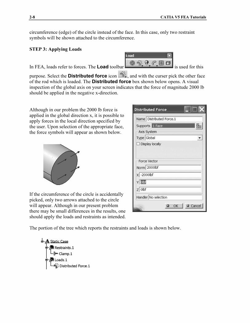
STEP 3: Applying Loads

In FEA, loads refer to forces. The Load toolbar is used for this

purpose. Select the Distributed force icon , and with the curser pick the other face

of the rod which is loaded. The Distributed force box shown below opens. A visual

inspection of the global axis on your screen indicates that the force of magnitude 2000 lb

should be applied in the negative x-direction.

Although in our problem the 2000 lb force is

applied in the global direction x, it is possible to

apply forces in the local direction specified by

the user. Upon selection of the appropriate face,

the force symbols will appear as shown below.

If the circumference of the circle is accidentally

picked, only two arrows attached to the circle

will appear. Although in our present problem

there may be small differences in the results, one

should apply the loads and restraints as intended.

The portion of the tree which reports the restraints and loads is shown below.


Copyrighted

Material


Copyrighted

Material


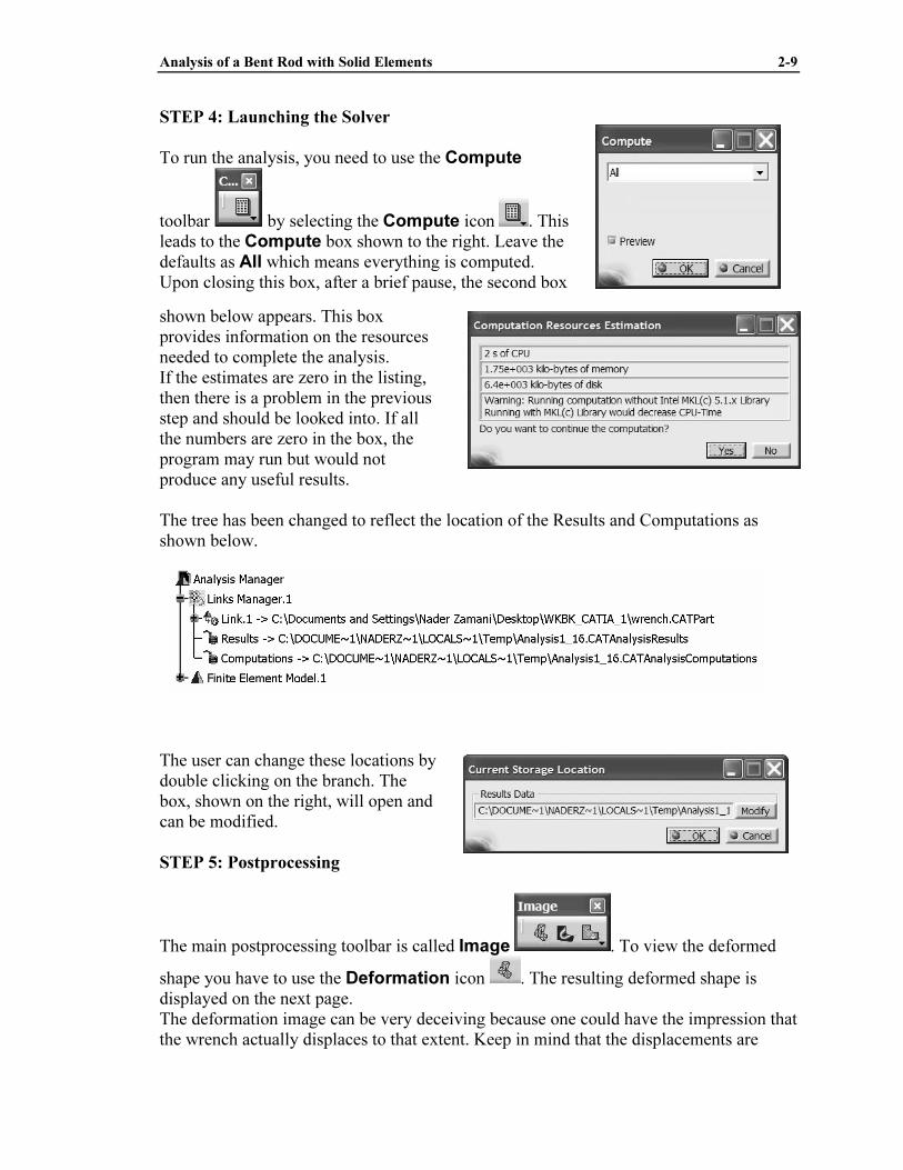
STEP 4: Launching the Solver

To run the analysis, you need to use the Compute

toolbar by selecting the Compute icon . This

leads to the Compute box shown to the right. Leave the

defaults as All which means everything is computed.

Upon closing this box, after a brief pause, the second box

shown below appears. This box

provides information on the resources

needed to complete the analysis.

If the estimates are zero in the listing,

then there is a problem in the previous

step and should be looked into. If all

the numbers are zero in the box, the

program may run but would not

produce any useful results.

The tree has been changed to reflect the location of the Results and Computations as

shown below.

The user can change these locations by

double clicking on the branch. The

box, shown on the right, will open and

can be modified.

STEP 5: Postprocessing

The main postprocessing toolbar is called Image . To view the deformed

shape you have to use the Deformation icon . The resulting deformed shape is

displayed on the next page.

The deformation image can be very deceiving because one could have the impression that

the wrench actually displaces to that extent. Keep in mind that the displacements are


Copyrighted

Material


Copyrighted

Material


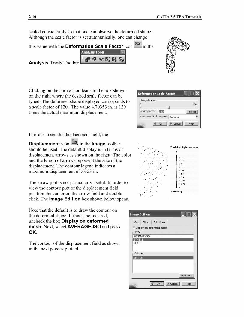
scaled considerably so that one can observe the deformed shape.

Although the scale factor is set automatically, one can change

this value with the Deformation Scale Factor icon in the

Analysis Tools Toolbar .

Clicking on the above icon leads to the box shown

on the right where the desired scale factor can be

typed. The deformed shape displayed corresponds to

a scale factor of 120. The value 4.70353 in. is 120

times the actual maximum displacement.

In order to see the displacement field, the

Displacement icon in the Image toolbar

should be used. The default display is in terms of

displacement arrows as shown on the right. The color

and the length of arrows represent the size of the

displacement. The contour legend indicates a

maximum displacement of .0353 in.

The arrow plot is not particularly useful. In order to

view the contour plot of the displacement field,

position the cursor on the arrow field and double

click. The Image Edition box shown below opens.

Note that the default is to draw the contour on

the deformed shape. If this is not desired,

uncheck the box Display on deformed mesh. Next, select AVERAGE-ISO and press

OK.

The contour of the displacement field as shown

in the next page is plotted.


Copyrighted

Material


Copyrighted

Material


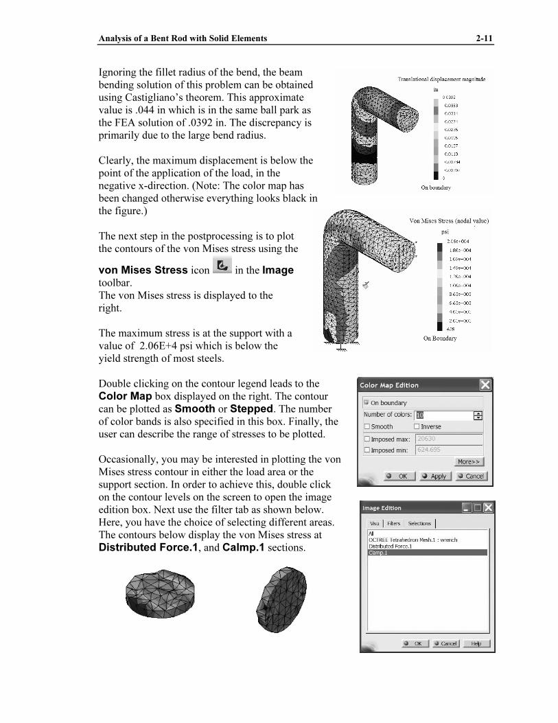
Ignoring the fillet radius of the bend, the beam

bending solution of this problem can be obtained

using Castigliano’s theorem. This approximate

value is .044 in which is in the same ball park as

the FEA solution of .0392 in. The discrepancy is

primarily due to the large bend radius.

Clearly, the maximum displacement is below the

point of the application of the load, in the

negative x-direction. (Note: The color map has

been changed otherwise everything looks black in

the figure.)

The next step in the postprocessing is to plot

the contours of the von Mises stress using the

von Mises Stress icon in the Image

toolbar.

The von Mises stress is displayed to the

right.

The maximum stress is at the support with a

value of 2.06E+4 psi which is below the

yield strength of most steels.

Double clicking on the contour legend leads to the

Color Map box displayed on the right. The contour

can be plotted as Smooth or Stepped. The number

of color bands is also specified in this box. Finally, the

user can describe the range of stresses to be plotted.

Occasionally, you may be interested in plotting the von

Mises stress contour in either the load area or the

support section. In order to achieve this, double click

on the contour levels on the screen to open the image

edition box. Next use the filter tab as shown below.

Here, you have the choice of selecting different areas.

The contours below display the von Mises stress at

Distributed Force.1, and Calmp.1 sections.


Copyrighted

Material


Copyrighted

Material


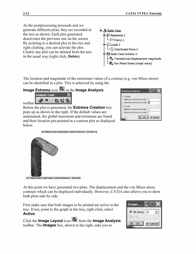
As the postprocessing proceeds and we

generate different plots, they are recorded in

the tree as shown. Each plot generated

deactivates the previous one on the screen.

By pointing to a desired plot in the tree and

right clicking, you can activate the plot.

Clearly any plot can be deleted from the tree

in the usual way (right click, Delete).

The location and magnitude of the extremum values of a contour (e.g. von Mises stress)

can be identified in a plot. This is achieved by using the

Image Extrema icon in the Image Analysis

toolbar .

Before the plot is generated, the Extrema Creation box

pops up as shown to the right. If the default values are

maintained, the global maximum and minimum are found

and their location pin-pointed in a contour plot as displayed

below.

At this point we have generated two plots. The displacement and the von Mises stress

contours which can be displayed individually. However, CATIA also allows you to show

both plots side by side.

First make sure that both images to be plotted are active in the

tree. If not, point to the graph in the tree, right click, select

Active.

Click the Image Layout icon from the Image Analysis

toolbar. The Images box, shown to the right, asks you to


Copyrighted

Material


Copyrighted

Material


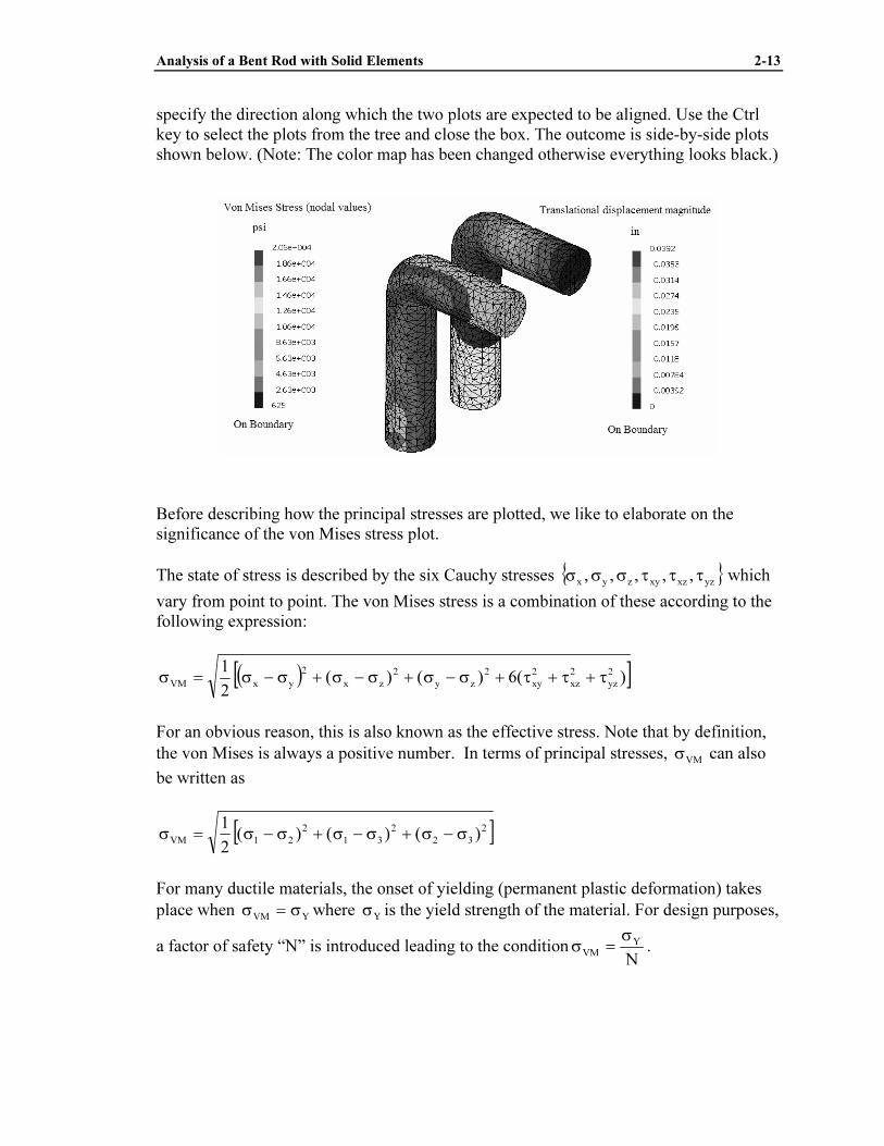
specify the direction along which the two plots are expected to be aligned. Use the Ctrl

key to select the plots from the tree and close the box. The outcome is side-by-side plots

shown below. (Note: The color map has been changed otherwise everything looks black.)

Before describing how the principal stresses are plotted, we like to elaborate on the

significance of the von Mises stress plot.

The state of stress is described by the six Cauchy stresses { }yzxzxyzyx

,,,,, τττσσσ which

vary from point to point. The von Mises stress is a combination of these according to the

following expression:

( )[ ])(6)()(2

1 2

yz

2

xz

2

xy

2

zy

2

zx

2

yxVM τ+τ+τ+σ−σ+σ−σ+σ−σ=σ

For an obvious reason, this is also known as the effective stress. Note that by definition,

the von Mises is always a positive number. In terms of principal stresses, VM

σ can also

be written as

[ ]232

2

31

2

21VM)()()(

2

1σ−σ+σ−σ+σ−σ=σ

For many ductile materials, the onset of yielding (permanent plastic deformation) takes

place when YVM

σ=σ where Y

σ is the yield strength of the material. For design purposes,

a factor of safety “N” is introduced leading to the conditionN

Y

VM

σ

=σ .


Copyrighted

Material


Copyrighted

Material


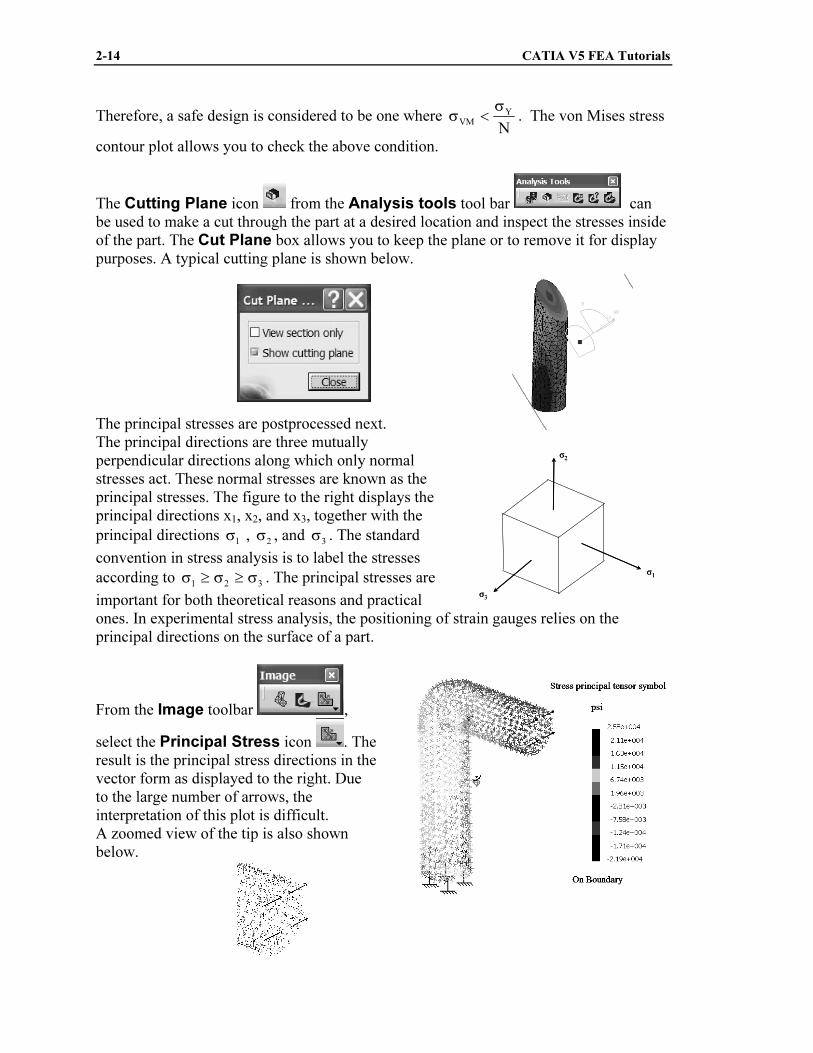
Therefore, a safe design is considered to be one where N

Y

VM

σ<σ . The von Mises stress

contour plot allows you to check the above condition.

The Cutting Plane icon from the Analysis tools tool bar can

be used to make a cut through the part at a desired location and inspect the stresses inside

of the part. The Cut Plane box allows you to keep the plane or to remove it for display

purposes. A typical cutting plane is shown below.

The principal stresses are postprocessed next.

The principal directions are three mutually

perpendicular directions along which only normal

stresses act. These normal stresses are known as the

principal stresses. The figure to the right displays the

principal directions x1, x2, and x3, together with the

principal directions 1

σ , 2

σ , and 3

σ . The standard

convention in stress analysis is to label the stresses

according to 321

σ≥σ≥σ . The principal stresses are

important for both theoretical reasons and practical

ones. In experimental stress analysis, the positioning of strain gauges relies on the

principal directions on the surface of a part.

From the Image toolbar ,

select the Principal Stress icon . The

result is the principal stress directions in the

vector form as displayed to the right. Due

to the large number of arrows, the

interpretation of this plot is difficult.

A zoomed view of the tip is also shown

below.

σ2

σ1

σ3

σ2

σ1

σ3


Copyrighted

Material


Copyrighted

Material


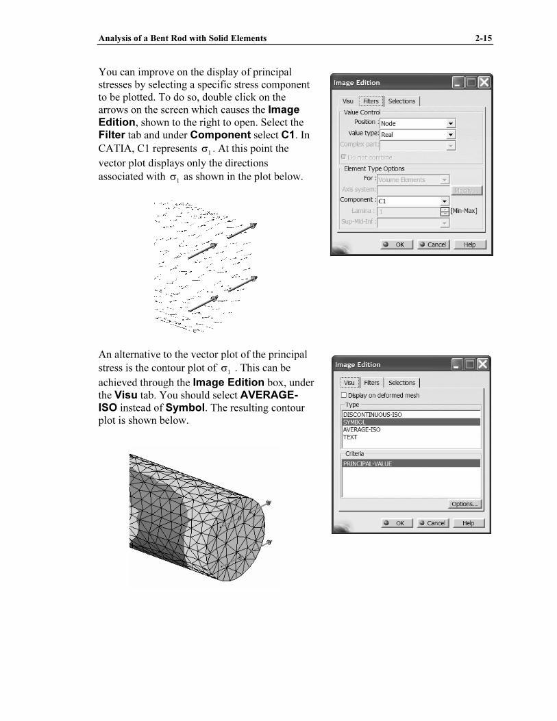
You can improve on the display of principal

stresses by selecting a specific stress component

to be plotted. To do so, double click on the

arrows on the screen which causes the Image Edition, shown to the right to open. Select the

Filter tab and under Component select C1. In

CATIA, C1 represents 1

σ . At this point the

vector plot displays only the directions

associated with 1

σ as shown in the plot below.

An alternative to the vector plot of the principal

stress is the contour plot of 1

σ . This can be

achieved through the Image Edition box, under

the Visu tab. You should select AVERAGE-ISO instead of Symbol. The resulting contour

plot is shown below.


Copyrighted

Material


Copyrighted

Material


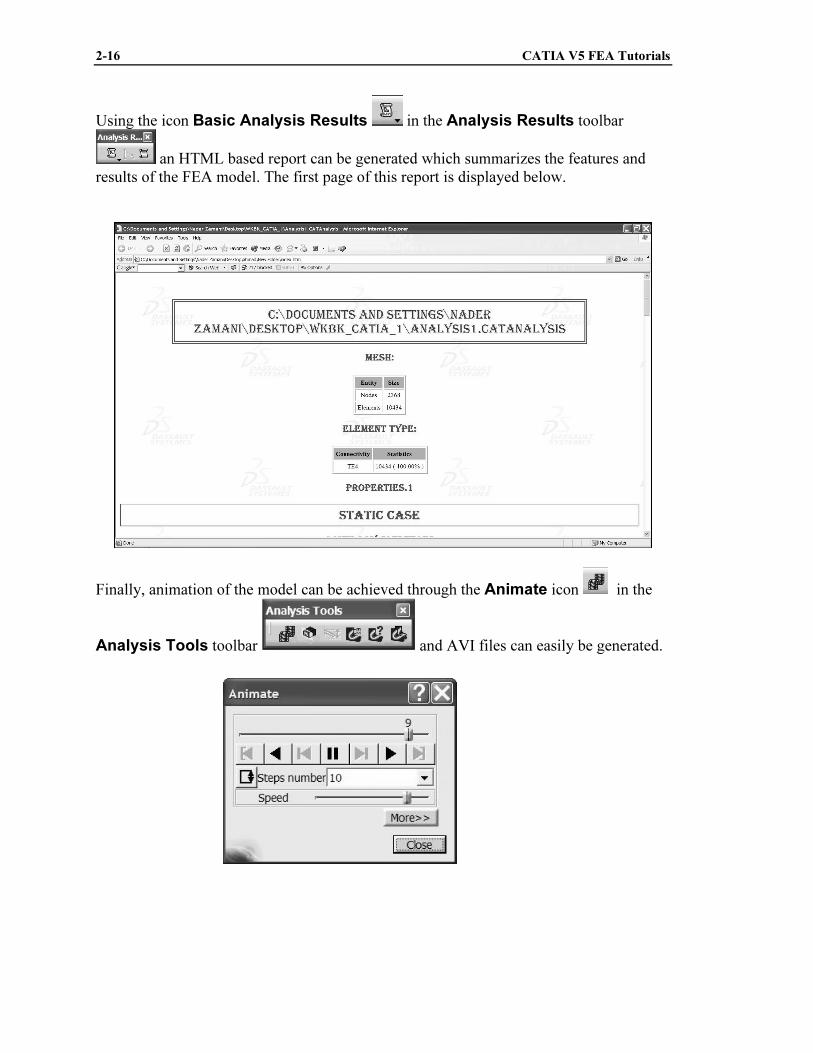
Using the icon Basic Analysis Results in the Analysis Results toolbar

an HTML based report can be generated which summarizes the features and

results of the FEA model. The first page of this report is displayed below.

Finally, animation of the model can be achieved through the Animate icon in the

Analysis Tools toolbar and AVI files can easily be generated.


Copyrighted

Material


Copyrighted

Material


Exercises for Chapter 2

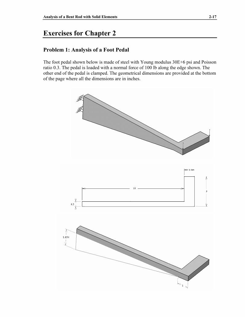
Problem 1: Analysis of a Foot Pedal

The foot pedal shown below is made of steel with Young modulus 30E+6 psi and Poisson

ratio 0.3. The pedal is loaded with a normal force of 100 lb along the edge shown. The

other end of the pedal is clamped. The geometrical dimensions are provided at the bottom

of the page where all the dimensions are in inches.


Copyrighted

Material


Copyrighted

Material


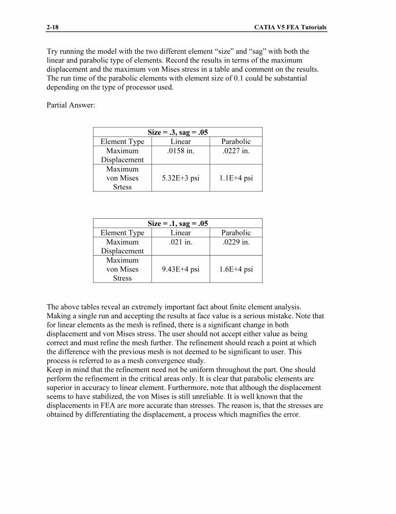
Try running the model with the two different element “size” and “sag” with both the

linear and parabolic type of elements. Record the results in terms of the maximum

displacement and the maximum von Mises stress in a table and comment on the results.

The run time of the parabolic elements with element size of 0.1 could be substantial

depending on the type of processor used.

Partial Answer:

Size = .3, sag = .05

Element Type Linear Parabolic

Maximum

Displacement

.0158 in. .0227 in.

Maximum

von Mises

Srtess

5.32E+3 psi

1.1E+4 psi

Size = .1, sag = .05

Element Type Linear Parabolic

Maximum

Displacement

.021 in. .0229 in.

Maximum

von Mises

Stress

9.43E+4 psi

1.6E+4 psi

The above tables reveal an extremely important fact about finite element analysis.

Making a single run and accepting the results at face value is a serious mistake. Note that

for linear elements as the mesh is refined, there is a significant change in both

displacement and von Mises stress. The user should not accept either value as being

correct and must refine the mesh further. The refinement should reach a point at which

the difference with the previous mesh is not deemed to be significant to user. This

process is referred to as a mesh convergence study.

Keep in mind that the refinement need not be uniform throughout the part. One should

perform the refinement in the critical areas only. It is clear that parabolic elements are

superior in accuracy to linear element. Furthermore, note that although the displacement

seems to have stabilized, the von Mises is still unreliable. It is well known that the

displacements in FEA are more accurate than stresses. The reason is, that the stresses are

obtained by differentiating the displacement, a process which magnifies the error.


Copyrighted

Material


Copyrighted

Material


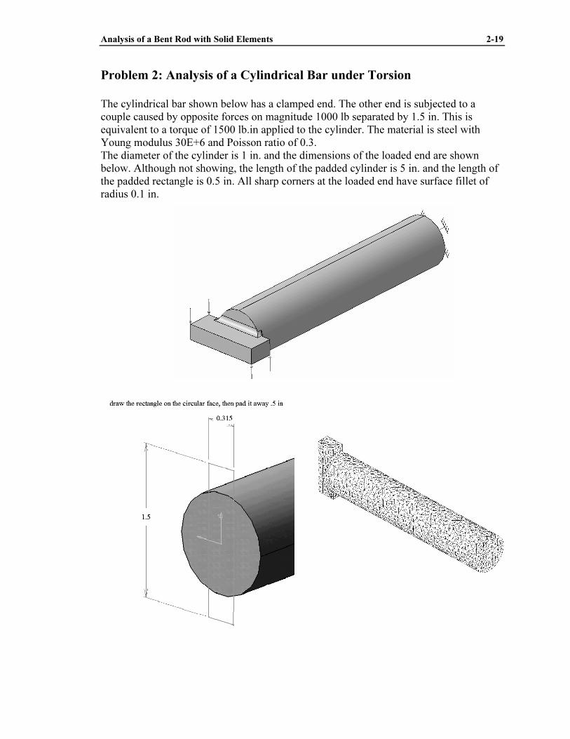
Problem 2: Analysis of a Cylindrical Bar under Torsion

The cylindrical bar shown below has a clamped end. The other end is subjected to a

couple caused by opposite forces on magnitude 1000 lb separated by 1.5 in. This is

equivalent to a torque of 1500 lb.in applied to the cylinder. The material is steel with

Young modulus 30E+6 and Poisson ratio of 0.3.

The diameter of the cylinder is 1 in. and the dimensions of the loaded end are shown

below. Although not showing, the length of the padded cylinder is 5 in. and the length of

the padded rectangle is 0.5 in. All sharp corners at the loaded end have surface fillet of

radius 0.1 in.


Copyrighted

Material


Copyrighted

Material


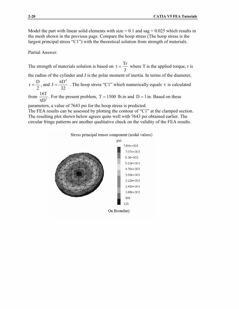
Model the part with linear solid elements with size = 0.1 and sag = 0.025 which results in

the mesh shown in the previous page. Compare the hoop stress (The hoop stress is the

largest principal stress “C1”) with the theoretical solution from strength of materials.

Partial Answer:

The strength of materials solution is based on J

Tr=τ where T is the applied torque, r is

the radius of the cylinder and J is the polar moment of inertia. In terms of the diameter,

2

Dr = , and

32

DJ

4π

= . The hoop stress “C1” which numerically equals τ is calculated

from 3

D

T16

π

. For the present problem, 1500T = lb.in and 1D = in. Based on these

parameters, a value of 7643 psi for the hoop stress is predicted.

The FEA results can be assessed by plotting the contour of “C1” at the clamped section.

The resulting plot shown below agrees quite well with 7643 psi obtained earlier. The

circular fringe patterns are another qualitative check on the validity of the FEA results.

catia v5 fea tutorials

Documents