case studies in trajectory optimization: trains, …rvdb/tex/trajopt/trajopt.pdfcase studies in...

CASE STUDIES IN TRAJECTORY OPTIMIZATION: TRAINS, PLANES, ANDOTHER PASTIMES

ROBERT J. VANDERBEI

Operations Research and Financial EngineeringPrinceton University

ORFE-00-3

Revised July 27, 2000

ABSTRACT. This is the first in a series of papers presenting case studies in modern large-scale constrained optimization, the purpose of which is to illustrate how recent advancesin algorithms and modeling languages have made it easy to solve difficult optimizationproblems using off-the-shelf software. In this first paper, we consider four trajectory opti-mization problems: (a) how to operate a train efficiently, (b) how to putt a golf ball on anuneven green so that it arrives at the cup with minimal speed, (c) how to fly a hang gliderso as to maximize or minimize the range of the glide, and (d) how to design a slide to makea toboggan go from beginning to end as quickly as possible.

In addition to the tutorial aspects of this paper, we also present evidence suggesting thatthe widely used trapezoidal discretization method is inferior in several ways to the simplermidpoint discretization method.

1. INTRODUCTION

This is the first in a series of papers presenting case studies in constrained optimization.The purpose of these studies is to illustrate how recent advances in algorithms and modelinglanguages now make it easy to solve once difficult optimization problems using off-the-shelve software. A secondary goal is to show that it is nonetheless still possible to makesubtle errors in a model which will render it (a) more difficult than it needs to be or (b)infeasible or, worse, (c) feasible but giving the wrong answer. In the past, many of theoptimization problems we present here were thought to be very difficult to solve and it was

Date: July 27, 2000.1991Mathematics Subject Classification.Primary 65L10 Secondary 34B15.Key words and phrases.trajectory optimization, optimal control, constrained optimization.Research supported by NSF grant DMS-9870317, ONR grant N00014-98-1-0036.

1

2 VANDERBEI

unclear whether failures were due to bad algorithms or bad models. Today, one can say thatfailures are almost always due to bad models.

In this paper we consider trajectory optimization problems. Our first example is abouthow to drive a train so as to minimize fuel costs. We follow this with two examples fromthe world of sports: golfing and flying. Subsequent papers in this series will treat appli-cations in electrical engineering (filter and antennae-array design) and in civil engineering(topology optimization of structures).

Throughout the paper we present several optimization models. We express these modelsin the AMPL modeling language [9]. This language provides a common mechanism forconveying problems to codes to solve them. When solving problems we generally use twodifferent codes: (a)LOQO [13, 14, 15, 2], which implements and interior-point method forgeneral nonlinear optimization and (b)SNOPT[10], which implements an active set strategyfor solving these problems.

2. TRAINS

An important problem in transportation is to minimize fuel costs in the operation of atrain. To keep things simple, we consider a segment of track that is straight although it maycontain hills and valleys. Letx denote position along the track measured from some fixedreference point. Lettingv denote the derivative of position with respect to time anda thetime-derivative ofv, we arrive at the following equations describing the motion of the train:

v = x

a = v

a = h(x)− (a + b|v|+ cv2) + ua − ub.(1)

Here,h(x) represents the acceleration/deceleration caused by going down/up hills,a, b,andc are constants so that the three termsa + b|v| + cv2 represent friction (both from thetrack and from the surrounding air),ua represents the acceleration provided by the engines,and ub represents the deceleration from applying the brakes. The control variables arethe functionsua andub. The objective is to take the train from one place given by initialcondition

x(0) = x0

v(0) = v0

to another given by

x(T ) = xf

v(T ) = vf

in such a way as to minimize fuel costs, which we take to be proportional to the totalamount of work done: ∫ T

0

ua(t)v(t)dt.

TRAINS, PLANES, AND OTHER PASTIMES 3

-2

-1.5

-1

-0.5

0

0.5

1

1.5

2

0 1 2 3 4 5 6

"train_g"

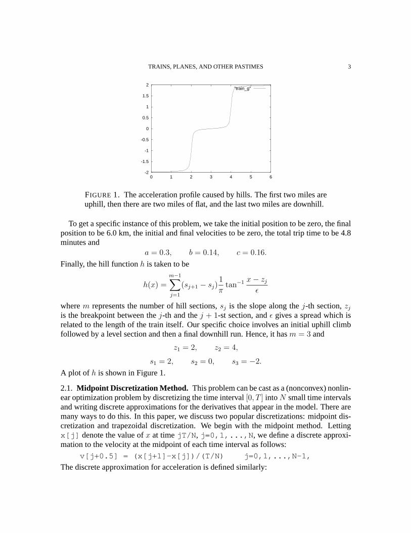
FIGURE 1. The acceleration profile caused by hills. The first two miles areuphill, then there are two miles of flat, and the last two miles are downhill.

To get a specific instance of this problem, we take the initial position to be zero, the finalposition to be 6.0 km, the initial and final velocities to be zero, the total trip time to be 4.8minutes and

a = 0.3, b = 0.14, c = 0.16.

Finally, the hill functionh is taken to be

h(x) =m−1∑j=1

(sj+1 − sj)1

πtan−1 x− zj

ε

wherem represents the number of hill sections,sj is the slope along thej-th section,zj

is the breakpoint between thej-th and thej + 1-st section, andε gives a spread which isrelated to the length of the train itself. Our specific choice involves an initial uphill climbfollowed by a level section and then a final downhill run. Hence, it hasm = 3 and

z1 = 2, z2 = 4,

s1 = 2, s2 = 0, s3 = −2.

A plot of h is shown in Figure 1.

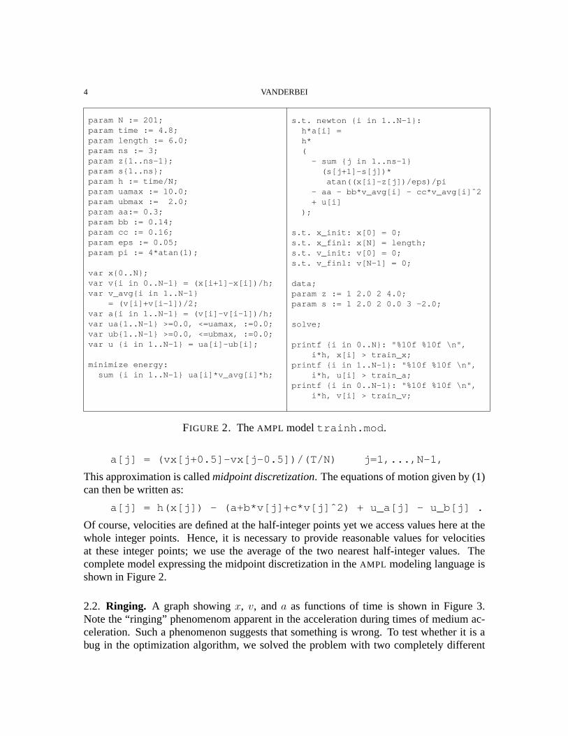
2.1. Midpoint Discretization Method. This problem can be cast as a (nonconvex) nonlin-ear optimization problem by discretizing the time interval[0, T ] into N small time intervalsand writing discrete approximations for the derivatives that appear in the model. There aremany ways to do this. In this paper, we discuss two popular discretizations: midpoint dis-cretization and trapezoidal discretization. We begin with the midpoint method. Lettingx[j] denote the value ofx at timejT/N , j=0,1,...,N , we define a discrete approxi-mation to the velocity at the midpoint of each time interval as follows:

v[j+0.5] = (x[j+1]-x[j])/(T/N) j=0,1,...,N-1,

The discrete approximation for acceleration is defined similarly:

4 VANDERBEI

param N := 201;param time := 4.8;param length := 6.0;param ns := 3;param z{1..ns-1};param s{1..ns};param h := time/N;param uamax := 10.0;param ubmax := 2.0;param aa:= 0.3;param bb := 0.14;param cc := 0.16;param eps := 0.05;param pi := 4*atan(1);

var x{0..N};var v{i in 0..N-1} = (x[i+1]-x[i])/h;var v_avg{i in 1..N-1}

= (v[i]+v[i-1])/2;var a{i in 1..N-1} = (v[i]-v[i-1])/h;var ua{1..N-1} >=0.0, <=uamax, :=0.0;var ub{1..N-1} >=0.0, <=ubmax, :=0.0;var u {i in 1..N-1} = ua[i]-ub[i];

minimize energy:sum {i in 1..N-1} ua[i]*v_avg[i]*h;

s.t. newton {i in 1..N-1}:h*a[i] =h*(

- sum {j in 1..ns-1}(s[j+1]-s[j])*

atan((x[i]-z[j])/eps)/pi- aa - bb*v_avg[i] - cc*v_avg[i]ˆ2+ u[i]

);

s.t. x_init: x[0] = 0;s.t. x_finl: x[N] = length;s.t. v_init: v[0] = 0;s.t. v_finl: v[N-1] = 0;

data;param z := 1 2.0 2 4.0;param s := 1 2.0 2 0.0 3 -2.0;

solve;

printf {i in 0..N}: "%10f %10f \n",i*h, x[i] > train_x;

printf {i in 1..N-1}: "%10f %10f \n",i*h, u[i] > train_a;

printf {i in 0..N-1}: "%10f %10f \n",i*h, v[i] > train_v;

FIGURE 2. TheAMPL modeltrainh.mod .

a[j] = (vx[j+0.5]-vx[j-0.5])/(T/N) j=1,...,N-1,

This approximation is calledmidpoint discretization. The equations of motion given by (1)can then be written as:

a[j] = h(x[j]) - (a+b*v[j]+c*v[j]ˆ2) + u_a[j] - u_b[j] .

Of course, velocities are defined at the half-integer points yet we access values here at thewhole integer points. Hence, it is necessary to provide reasonable values for velocitiesat these integer points; we use the average of the two nearest half-integer values. Thecomplete model expressing the midpoint discretization in theAMPL modeling language isshown in Figure 2.

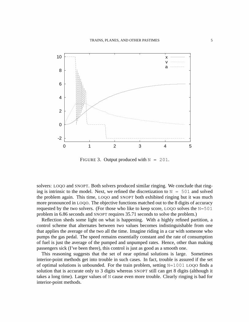
2.2. Ringing. A graph showingx, v, anda as functions of time is shown in Figure 3.Note the “ringing” phenomenom apparent in the acceleration during times of medium ac-celeration. Such a phenomenon suggests that something is wrong. To test whether it is abug in the optimization algorithm, we solved the problem with two completely different


-2

0

2

4

6

8

10

0 1 2 3 4 5

xva

FIGURE 3. Output produced withN = 201.

solvers:LOQO andSNOPT. Both solvers produced similar ringing. We conclude that ring-ing is intrinsic to the model. Next, we refined the discretization toN = 501 and solvedthe problem again. This time,LOQO andSNOPT both exhibited ringing but it was muchmore pronounced inLOQO. The objective functions matched out to the 8 digits of accuracyrequested by the two solvers. (For those who like to keep score,LOQO solves theN=501problem in 6.86 seconds andSNOPTrequires 35.71 seconds to solve the problem.)

Reflection sheds some light on what is happening. With a highly refined partition, acontrol scheme that alternates between two values becomes indistinguishable from onethat applies the average of the two all the time. Imagine riding in a car with someone whopumps the gas pedal. The speed remains essentially constant and the rate of consumptionof fuel is just the average of the pumped and unpumped rates. Hence, other than makingpassengers sick (I’ve been there), this control is just as good as a smooth one.

This reasoning suggests that the set of near optimal solutions is large. Sometimesinterior-point methods get into trouble in such cases. In fact, trouble is assured if the setof optimal solutions is unbounded. For the train problem, settingN=1001 LOQO finds asolution that is accurate only to 3 digits whereasSNOPTstill can get 8 digits (although ittakes a long time). Larger values ofN cause even more trouble. Clearly ringing is bad forinterior-point methods.

6 VANDERBEI

-2

0

2

4

6

8

10

0 1 2 3 4 5

xva

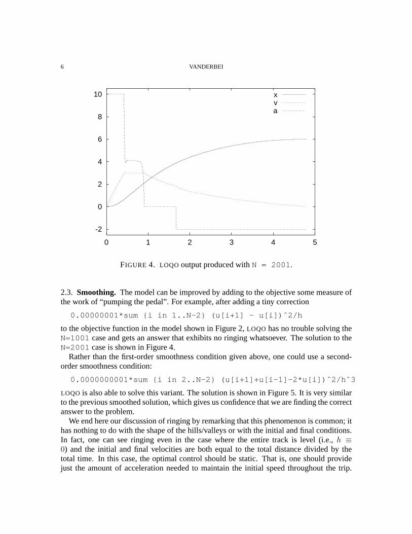
FIGURE 4. LOQO output produced withN = 2001.

2.3. Smoothing. The model can be improved by adding to the objective some measure ofthe work of “pumping the pedal”. For example, after adding a tiny correction

0.00000001*sum {i in 1..N-2} (u[i+1] - u[i])ˆ2/h

to the objective function in the model shown in Figure 2,LOQO has no trouble solving theN=1001 case and gets an answer that exhibits no ringing whatsoever. The solution to theN=2001 case is shown in Figure 4.

Rather than the first-order smoothness condition given above, one could use a second-order smoothness condition:

0.0000000001*sum {i in 2..N-2} (u[i+1]+u[i-1]-2*u[i])ˆ2/hˆ3

LOQO is also able to solve this variant. The solution is shown in Figure 5. It is very similarto the previous smoothed solution, which gives us confidence that we are finding the correctanswer to the problem.

We end here our discussion of ringing by remarking that this phenomenon is common; ithas nothing to do with the shape of the hills/valleys or with the initial and final conditions.In fact, one can see ringing even in the case where the entire track is level (i.e.,h ≡0) and the initial and final velocities are both equal to the total distance divided by thetotal time. In this case, the optimal control should be static. That is, one should providejust the amount of acceleration needed to maintain the initial speed throughout the trip.


-2

0

2

4

6

8

10

0 1 2 3 4 5

xva

FIGURE 5. LOQO output produced withN = 2001.

But, without the smoothing terms mentioned above, bothLOQO andSNOPTfind nonstaticringing-type solutions.

2.4. Trapezoidal Discretization. We end this section with a description of the secondcommon method for discretizing first-order differential equations. This method is calledthetrapezoidal discretization. With this discretization, values forv anda are defined at thesame discrete times as forx ; that is, atjT/N , j=0,1,...,N . Instead of giving a formuladefining each velocity in terms of a difference of positions, we give constraints that saythat the average value of the values ofv at two adjacent times is equal to the appropriatedifference in the positional values:

(v[j+1]+v[j])/2 = (x[j+1]-x[j])/(T/N) j=0,1,...,N-1,

Constraints that must be satisfied by the accelerations are similar:

(a[j+1]+a[j])/2 = (v[j+1]-v[j])/(T/N) j=0,1,...,N-1,

The model in its entirety is shown in Figure 6. Generally speaking trapezoidal discretiza-tions are more popular than their midpoint counterparts, but there are drawbacks.

First of all, for the train models that we are considering the midpoint method is lessaffected by the ringing phenomenon. This is seen from the fact that the1.0e-8 factorused in the midpoint method has to be increased to1.0e-6 in the trapezoidal methodbeforeLOQO can solve the model. Furthermore, even with this larger smoothing factor, themidpoint model solves in 83 iterations whereas the trapezoidal model requires 187.

8 VANDERBEI

param N := 2001;param time := 4.8;param length := 6.0;param ns := 3;param z{1..ns-1} ;param s{1..ns} ;param h := time/N;param uamax := 10.0;param ubmax := 2.0;param aa:= 0.3;param bb := 0.14;param cc := 0.16;param eps := 0.05;param pi := 4*atan(1);

var x{0..N};var v{0..N};var a{0..N};var ua{0..N} >= 0.0, <= uamax, := 0.0;var ub{0..N} >= 0.0, <= ubmax, := 0.0;var u {i in 0..N} = ua[i] - ub[i];

minimize energy:sum {i in 0..N} ua[i]*v[i]*h+ 0.000001*sum {i in 0..N-1}

(u[i+1] - u[i])ˆ2/h;

s.t. v_def {i in 0..N-1}:(v[i+1]+v[i])/2 = (x[i+1]-x[i])/h;

s.t. a_def {i in 0..N-1}:(a[i+1]+a[i])/2 = (v[i+1]-v[i])/h;

s.t. newton {i in 0..N}:h*a[i] =h*(- sum {j in 1..ns-1}

(s[j+1]-s[j])*atan((x[i]-z[j])/eps)/pi

- aa - bb*v[i] - cc*v[i]ˆ2+ u[i]);

s.t. x_init: x[0] = 0;s.t. x_finl: x[N] = length;s.t. v_init: v[0] = 0;s.t. v_finl: v[N] = 0;

data;param z := 1 2.0 2 4.0;param s := 1 2.0 2 0.0 3 -2.0;

solve;

printf {i in 0..N}: "%10f %10f \n",i*h, x[i] > train_x;

printf {i in 0..N}: "%10f %10f \n",i*h, v[i] > train_v;

printf {i in 0..N}: "%10f %10f \n",i*h, u[i] > train_a;

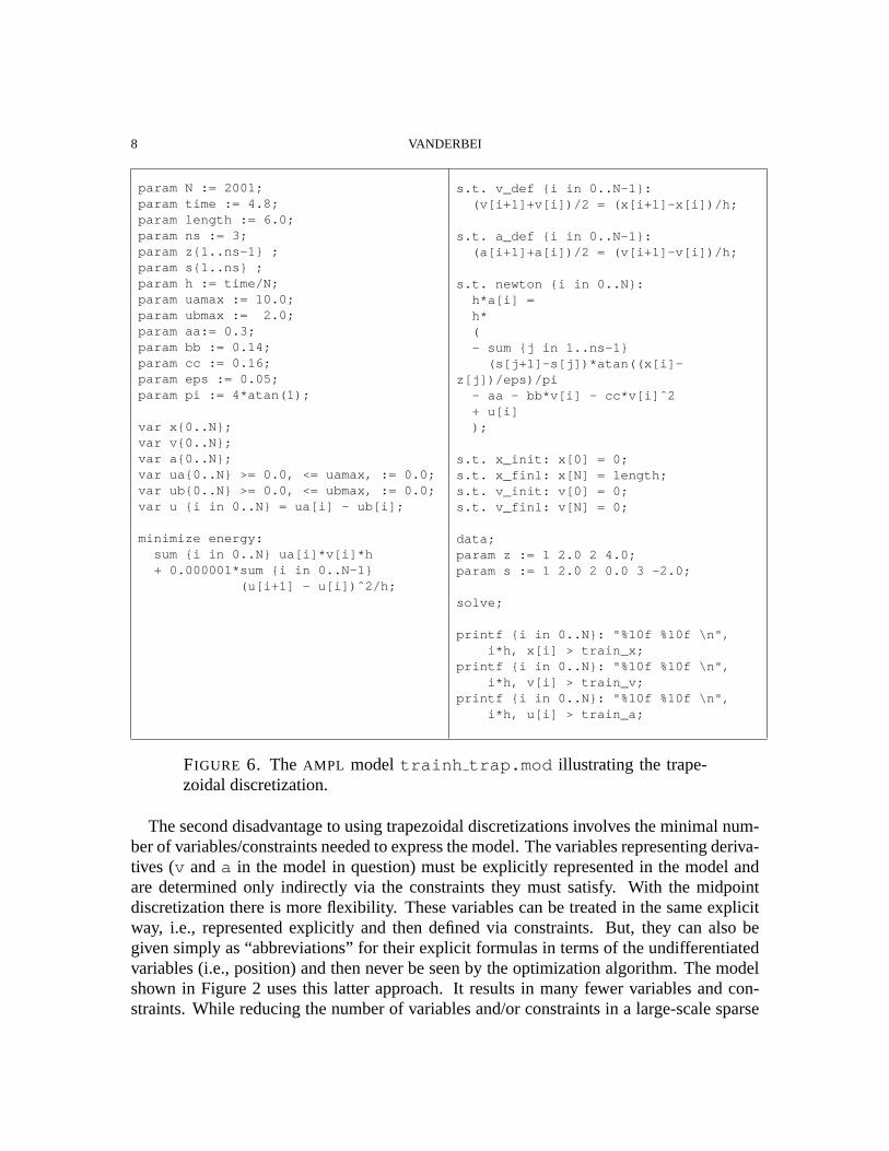
FIGURE 6. TheAMPL model trainh trap.mod illustrating the trape-zoidal discretization.

The second disadvantage to using trapezoidal discretizations involves the minimal num-ber of variables/constraints needed to express the model. The variables representing deriva-tives (v anda in the model in question) must be explicitly represented in the model andare determined only indirectly via the constraints they must satisfy. With the midpointdiscretization there is more flexibility. These variables can be treated in the same explicitway, i.e., represented explicitly and then defined via constraints. But, they can also begiven simply as “abbreviations” for their explicit formulas in terms of the undifferentiatedvariables (i.e., position) and then never be seen by the optimization algorithm. The modelshown in Figure 2 uses this latter approach. It results in many fewer variables and con-straints. While reducing the number of variables and/or constraints in a large-scale sparse


optimization problem does not always mean faster solution times, it often does and that isthe case here. ForN=2001, the midpoint model has 5998 variables, 2000 constraints, andsolves in 86 seconds (using 83 iterations of the basic algorithm). On the other hand, thetrapezoidal model has 10006 variables, 6004 constraints, and solves in 355 seconds (using187 iterations). More iterations are needed because, as stated earlier, this method suffersmore from ringing but even on a per iteration basis the midpoint model solves twice as fast.

The trapezoidal discretization of the train model that we’ve studied here derives from themodeltrainh in theCUTE [8] suite on test problems. TheCUTE model was itself adaptedfrom a paper by Kautsky and Nichols [11].

2.5. Lessons.After studying hundreds of nonlinear optimization problems, we have learnedmany lessons about how to formulate models appropriately and what type of algorithm willsolve these problems efficiently and robustly. While a single example is not sufficient fordeducing these lessons, it can be used to illustrate them. The lessons illustrated by the trainproblem can be summarized as follows:

(1) Discrete approximations to continuous problems can exhibit unexpected patholog-ical behaviour such as the ringing we saw here.

(2) Optimization problems with large sets of optimal (or nearly optimal) solutions canpresent numerical difficulties for interior-point methods.

(3) Interior-point methods are often more efficient than active-set methods on largeproblems.

(4) Midpoint discretizations have fewer degrees of freedom than trapezoidal discretiza-tions and therefore are less likely to exhibit ringing.

(5) With midpoint discretization one can eliminate the higher-order derivatives fromthe optimization model producing a reduced model that may solve more efficientlythan the expanded version.

3. PUTTING

The problem of how to putt provides a simple framework to continue our discussion oftrajectory optimization. One of the lessons to be learned with this example is how easy itis to make a wrong model. With this in mind, we advise the interested golfer to read theentire section because the first model, right as it may appear, is wrong.

3.1. The Alessandrini Model. We begin with a discussion of the problem essentially asit appears in [1].

Given a golf ball sitting at rest on a putting green, the problem is to figure out how to hitthe ball so that it will go into the cup. To make sure that it does not just skim over the cupand stop at some point far beyond, we try to have the ball arrive at the cup with the smallestmomentum possible.

The Normal Vector.We assume that the elevation of the green is given as(x, y, z(x, y))together and that its shape is given by(x/a)2 + (y/b)2 ≤ 1. Two tangent vectors to the

10 VANDERBEI

surface are provided by(1, 0, ∂z/∂x) and (0, 1, ∂z/∂y). By taking the cross product ofthese two vectors, we obtain an upward pointing normal vector to the surface:

(−∂z/∂x,−∂z/∂y, 1).

The normal forceN exerted by the surface of the green on the golf ball must point in thisdirection and its magnitude must be such that the total force in this direction vanishes (tokeep the ball rolling on the surface).

The Normal Force.Since the only forces that are not tangential to the green are the forceof gravity and the normal force itself, we must have the projection of the force of gravityon the normal direction be exactly opposite to the magnitude of the normal force:

−mg(ez ·N)/‖N‖ = −‖N‖,

wherem is mass of the ball,g is acceleration due to gravity,ez is the unit vector pointingin the vertical direction, and of courseN is proportional to the normal vector given above.From this relation, we get that

Nz =mg

(∂z/∂x)2 + (∂z/∂y)2 + 1

and thatNx = −∂z/∂xNz Ny = −∂z/∂yNz.

Friction. There is friction between the ball and the green. It is assumed to be proportionalto the normal force and to point in a direction opposite to the velocity:

F = −µ‖N‖ v

‖v‖.

Equations of Motion.If we denote the trajectory byu(t) = (x(t), y(t), z(t)), then theequations of motion are

v = u

a = v

ma = N + F −mgez.(2)

Boundary Conditions.The initial and final positions are known,

u(0) = u0 and u(T ) = uf ,

but the timeT at which the final position is reached is a variable.As with the train example, this problem can be cast as a (nonconvex) nonlinear optimiza-

tion problem using either a midpoint or a trapezoidal discretization rule. Inspired by ourlesson from the previous example indicating some advantages to the midpoint rule, we startwith this method. We discuss the trapzoidal rule at the end of this section.

Using the midpoint rule, we can letx[j] , y[j] , andz[j] denote the positional co-ordinates at timejT/N , j=0,1,...,N , and then define discrete approximations to thethree components of velocity at the midpoint of each time interval as follows:


vx[j+0.5] = (x[j+1]-x[j])/(T/N) j=0,1,...,N-1,vy[j+0.5] = (y[j+1]-y[j])/(T/N) j=0,1,...,N-1,vz[j+0.5] = (z[j+1]-z[j])/(T/N) j=0,1,...,N-1.

Discrete approximations for acceleration are defined similarly:ax[j] = (vx[j+0.5]-vx[j-0.5])/(T/N) j=1,...,N-1,ay[j] = (vy[j+0.5]-vy[j-0.5])/(T/N) j=1,...,N-1,az[j] = (vz[j+0.5]-vz[j-0.5])/(T/N) j=1,...,N-1.

The equations of motion given by (2) complete the constraints defining the model:ax[j] = (Nx[j] + Fr_x[j])/m,ay[j] = (Ny[j] + Fr_y[j])/m,az[j] = (Nz[j] + Fr_z[j])/m - g.

Here,Nx[j] , Ny[j] , andNz[j] are shorthand forNz[j] = m*g/(dzdx[j]ˆ2 + dzdy[j]ˆ2 + 1),Nx[j] = -dzdx[j]*Nz[j],Ny[j] = -dzdy[j]*Nz[j]

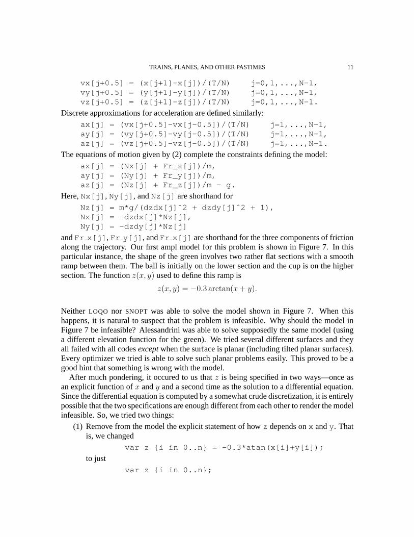
andFr x[j] , Fr y[j] , andFr x[j] are shorthand for the three components of frictionalong the trajectory. Our first ampl model for this problem is shown in Figure 7. In thisparticular instance, the shape of the green involves two rather flat sections with a smoothramp between them. The ball is initially on the lower section and the cup is on the highersection. The functionz(x, y) used to define this ramp is

z(x, y) = −0.3 arctan(x + y).

Neither LOQO nor SNOPT was able to solve the model shown in Figure 7. When thishappens, it is natural to suspect that the problem is infeasible. Why should the model inFigure 7 be infeasible? Alessandrini was able to solve supposedly the same model (usinga different elevation function for the green). We tried several different surfaces and theyall failed with all codesexceptwhen the surface is planar (including tilted planar surfaces).Every optimizer we tried is able to solve such planar problems easily. This proved to be agood hint that something is wrong with the model.

After much pondering, it occured to us thatz is being specified in two ways—once asan explicit function ofx andy and a second time as the solution to a differential equation.Since the differential equation is computed by a somewhat crude discretization, it is entirelypossible that the two specifications are enough different from each other to render the modelinfeasible. So, we tried two things:

(1) Remove from the model the explicit statement of howz depends onx andy . Thatis, we changed

var z {i in 0..n} = -0.3*atan(x[i]+y[i]);

to justvar z {i in 0..n};

12 VANDERBEI

param g := 9.8; # acc due to gravityparam m := 0.01; # mass of a golf ballparam x0 := 1; # coords of start ptparam y0 := 2;param xn := 1; # coords of ending ptparam yn := -2;param n := 50; # num of time pointsparam mu;

var T >= 0; # total time for the puttvar x{0..n}; # coords of the trajvar y{0..n};

var z {i in 0..n}= -0.3*atan(x[i]+y[i]);

var dzdx{i in 0..n}= -0.3/(1+(x[i]+y[i])ˆ2);

var dzdy{i in 0..n}= -0.3/(1+(x[i]+y[i])ˆ2);

# v[i] denotes the deriv at midpt of# the interval i(T/n) to (i+1)(T/n).var vx{i in 0..n-1} = (x[i+1]-x[i])*n/T;var vy{i in 0..n-1} = (y[i+1]-y[i])*n/T;var vz{i in 0..n-1} = (z[i+1]-z[i])*n/T;

# a[i] denotes the accel at midpt of# the interval (i-0.5)(T/n)# to (i+0.5)(T/n), i.e. at i(T/n).var ax{i in 1..n-1} = (vx[i]-vx[i-1])*n/T;var ay{i in 1..n-1} = (vy[i]-vy[i-1])*n/T;var az{i in 1..n-1} = (vz[i]-vz[i-1])*n/T;

var Nz{i in 1..n-1}= m*g/(dzdx[i]ˆ2 + dzdy[i]ˆ2 + 1);

var Nx{i in 1..n-1} = -dzdx[i]*Nz[i];var Ny{i in 1..n-1} = -dzdy[i]*Nz[i];var Nmag{i in 1..n-1}

= m*g/sqrt(dzdx[i]ˆ2 + dzdy[i]ˆ2 + 1);

var vx_avg{i in 1..n-1}= (vx[i]+vx[i-1])/2;

var vy_avg{i in 1..n-1}= (vy[i]+vy[i-1])/2;

var vz_avg{i in 1..n-1}= (vz[i]+vz[i-1])/2;

var speed{i in 1..n-1}= sqrt(vx_avg[i]ˆ2 + vy_avg[i]ˆ2

+ vz_avg[i]ˆ2);

var Frx{i in 1..n-1}= -mu*Nmag[i]*vx_avg[i]/speed[i];

var Fry{i in 1..n-1}= -mu*Nmag[i]*vy_avg[i]/speed[i];

var Frz{i in 1..n-1}= -mu*Nmag[i]*vz_avg[i]/speed[i];

minimize finalspeed:vx[n-1]ˆ2 + vy[n-1]ˆ2;

s.t. newt_x {i in 1..n-1}:ax[i] = (Nx[i] + Frx[i])/m;

s.t. newt_y {i in 1..n-1}:ay[i] = (Ny[i] + Fry[i])/m;

s.t. newt_z {i in 1..n-1}:az[i] = (Nz[i] + Frz[i] - m*g)/m;

s.t. xinit: x[0] = x0;s.t. yinit: y[0] = y0;s.t. zinit: z[0]

= -0.3*atan(x[0]+y[0]);

s.t. xfinal: x[n] = xn;s.t. yfinal: y[n] = yn;s.t. zfinal: z[n]

= -0.3*atan(x[n]+y[n]);

s.t. onthegreen {i in 0..n}:x[i]ˆ2 + y[i]ˆ2 <= 16;

let T := 1.5;

let mu := 0.2;let {i in 0..n}

y[i] := (i/n)*yn + (1-i/n)*y0;let {i in 0..n}

x[i] := y[i]ˆ2/2;

let mu := 0.25;solve;

FIGURE 7. A first AMPL model for the putting problem.

(2) Remove from the model the part of the differential equation that relates to thezcomponent of the trajectory. That is, we removed the constraintsnewt z , zinit ,andzfinal .


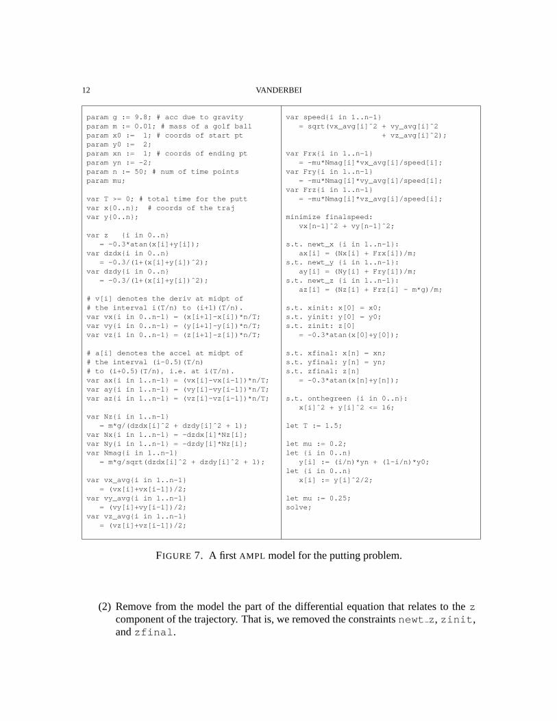
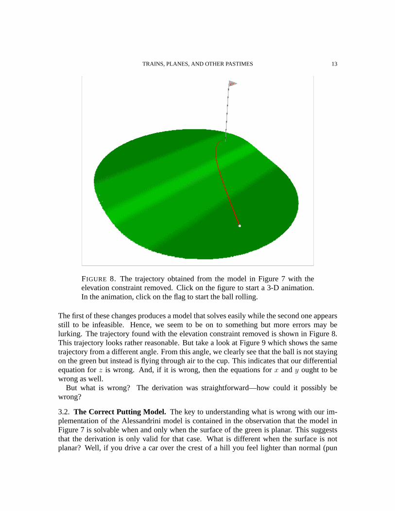
FIGURE 8. The trajectory obtained from the model in Figure 7 with theelevation constraint removed. Click on the figure to start a 3-D animation.In the animation, click on the flag to start the ball rolling.

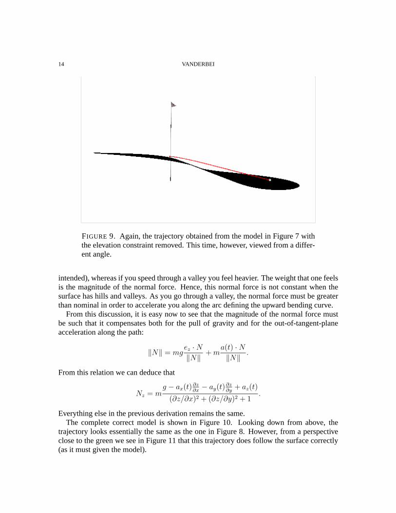
The first of these changes produces a model that solves easily while the second one appearsstill to be infeasible. Hence, we seem to be on to something but more errors may belurking. The trajectory found with the elevation constraint removed is shown in Figure 8.This trajectory looks rather reasonable. But take a look at Figure 9 which shows the sametrajectory from a different angle. From this angle, we clearly see that the ball is not stayingon the green but instead is flying through air to the cup. This indicates that our differentialequation forz is wrong. And, if it is wrong, then the equations forx andy ought to bewrong as well.

But what is wrong? The derivation was straightforward—how could it possibly bewrong?

3.2. The Correct Putting Model. The key to understanding what is wrong with our im-plementation of the Alessandrini model is contained in the observation that the model inFigure 7 is solvable when and only when the surface of the green is planar. This suggeststhat the derivation is only valid for that case. What is different when the surface is notplanar? Well, if you drive a car over the crest of a hill you feel lighter than normal (pun

http://www.princeton.edu/~rvdb/tex/trajopt/putt/puttwrong.wrl

14 VANDERBEI

FIGURE 9. Again, the trajectory obtained from the model in Figure 7 withthe elevation constraint removed. This time, however, viewed from a differ-ent angle.

intended), whereas if you speed through a valley you feel heavier. The weight that one feelsis the magnitude of the normal force. Hence, this normal force is not constant when thesurface has hills and valleys. As you go through a valley, the normal force must be greaterthan nominal in order to accelerate you along the arc defining the upward bending curve.

From this discussion, it is easy now to see that the magnitude of the normal force mustbe such that it compensates both for the pull of gravity and for the out-of-tangent-planeacceleration along the path:

‖N‖ = mgez ·N‖N‖

+ ma(t) ·N‖N‖

.

From this relation we can deduce that

Nz = mg − ax(t)

∂z∂x− ay(t)

∂z∂y

+ az(t)

(∂z/∂x)2 + (∂z/∂y)2 + 1.

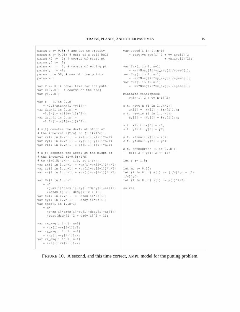
Everything else in the previous derivation remains the same.The complete correct model is shown in Figure 10. Looking down from above, the

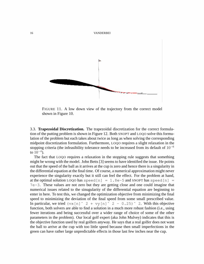
trajectory looks essentially the same as the one in Figure 8. However, from a perspectiveclose to the green we see in Figure 11 that this trajectory does follow the surface correctly(as it must given the model).

http://www.princeton.edu/~rvdb/tex/trajopt/putt/puttwrong.wrl





var dzdx{i in 0..n} =-0.3/(1+(x[i]+y[i])ˆ2);

var dzdy{i in 0..n} =-0.3/(1+(x[i]+y[i])ˆ2);

# v[i] denotes the deriv at midpt of# the interval i(T/n) to (i+1)(T/n).var vx{i in 0..n-1} = (x[i+1]-x[i])*n/T;var vy{i in 0..n-1} = (y[i+1]-y[i])*n/T;var vz{i in 0..n-1} = (z[i+1]-z[i])*n/T;

# a[i] denotes the accel at the midpt of# the interval (i-0.5)(T/n)# to (i+0.5)(T/n), i.e. at i(T/n).var ax{i in 1..n-1} = (vx[i]-vx[i-1])*n/T;var ay{i in 1..n-1} = (vy[i]-vy[i-1])*n/T;var az{i in 1..n-1} = (vz[i]-vz[i-1])*n/T;

var Nz{i in 1..n-1}= m*

(g-ax[i]*dzdx[i]-ay[i]*dzdy[i]+az[i])/(dzdx[i]ˆ2 + dzdy[i]ˆ2 + 1);

var Nx{i in 1..n-1} = -dzdx[i]*Nz[i];var Ny{i in 1..n-1} = -dzdy[i]*Nz[i];var Nmag{i in 1..n-1}

= m*(g-ax[i]*dzdx[i]-ay[i]*dzdy[i]+az[i])/sqrt(dzdx[i]ˆ2 + dzdy[i]ˆ2 + 1);

var vx_avg{i in 1..n-1}= (vx[i]+vx[i-1])/2;

var vy_avg{i in 1..n-1}= (vy[i]+vy[i-1])/2;

var vz_avg{i in 1..n-1}= (vz[i]+vz[i-1])/2;

var speed{i in 1..n-1}= sqrt(vx_avg[i]ˆ2 + vy_avg[i]ˆ2

+ vz_avg[i]ˆ2);

var Frx{i in 1..n-1}= -mu*Nmag[i]*vx_avg[i]/speed[i];

var Fry{i in 1..n-1}= -mu*Nmag[i]*vy_avg[i]/speed[i];

var Frz{i in 1..n-1}= -mu*Nmag[i]*vz_avg[i]/speed[i];

minimize finalspeed:vx[n-1]ˆ2 + vy[n-1]ˆ2;

s.t. newt_x {i in 1..n-1}:ax[i] = (Nx[i] + Frx[i])/m;

s.t. newt_y {i in 1..n-1}:ay[i] = (Ny[i] + Fry[i])/m;

s.t. xinit: x[0] = x0;s.t. yinit: y[0] = y0;

s.t. xfinal: x[n] = xn;s.t. yfinal: y[n] = yn;


let T := 1.5;

let mu := 0.25;let {i in 0..n} y[i] := (i/n)*yn + (1-i/n)*y0;let {i in 0..n} x[i] := y[i]ˆ2/2;

solve;

FIGURE 10. A second, and this time correct,AMPL model for the putting problem.

16 VANDERBEI

FIGURE 11. A low down view of the trajectory from the correct modelshown in Figure 10.

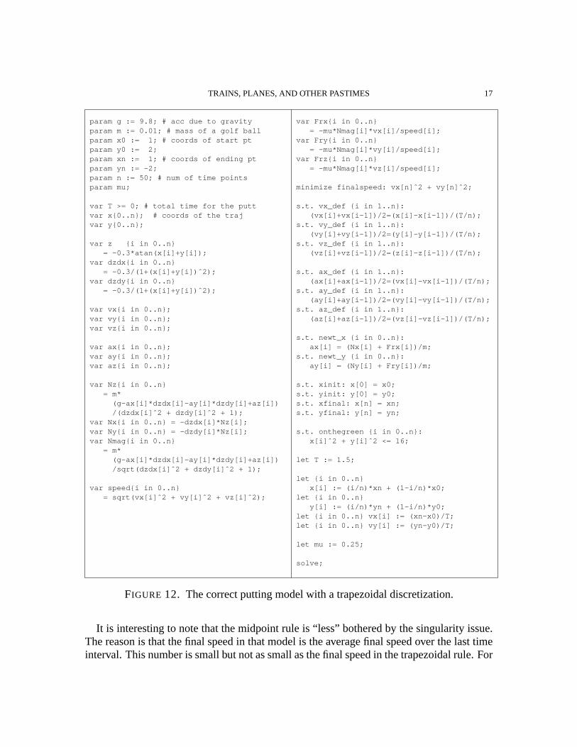
3.3. Trapezoidal Discretization. The trapezoidal discretization for the correct formula-tion of the putting problem is shown in Figure 12. BothSNOPTandLOQO solve this formu-lation of the problem but each takes about twice as long as when solving the correspondingmidpoint discretization formulation. Furthermore,LOQO requires a slight relaxation in thestopping criteria (the infeasibility tolerance needs to be increased from its default of10−6

to 10−4).The fact thatLOQO requires a relaxation in the stopping rule suggests that something

might be wrong with the model. John Betts [3] seems to have identified the issue. He pointsout that the speed of the ball as it arrives at the cup is zero and hence there is a singularity inthe differential equation at the final time. Of course, a numerical approximation might neverexperience the singularity exactly but it still can feel the effect. For the problem at hand,at the optimal solutionLOQO hasspeed[n] = 1.8e-5 andSNOPThasspeed[n] =7e-3 . These values are not zero but they are getting close and one could imagine thatnumerical issues related to the sinugularity of the differential equation are beginning toenter in here. To test this, we changed the optimization objective from minimizing the finalspeed to minimizing the deviation of the final speed from some small prescribed value.In particular, we tried(vx[n]ˆ 2 + vy[n]ˆ 2 - 0.25)ˆ 2 . With this objectivefunction, both solvers are able to find a solution in a much more robust fashion (i.e., usingfewer iterations and being successful over a wider range of choice of some of the otherparameters in the problem). Our local golf expert (aka John Mulvey) indicates that this isthe objective function used by real golfers anyway. He says that a real golfer does not wantthe ball to arrive at the cup with too little speed because then small imperfections in thegreen can have rather large unpredictable effects in those last few inches near the cup.

http://www.princeton.edu/~rvdb/tex/trajopt/putt/putt.wrl





var dzdx{i in 0..n}= -0.3/(1+(x[i]+y[i])ˆ2);

var dzdy{i in 0..n}= -0.3/(1+(x[i]+y[i])ˆ2);

var vx{i in 0..n};var vy{i in 0..n};var vz{i in 0..n};

var ax{i in 0..n};var ay{i in 0..n};var az{i in 0..n};

var Nz{i in 0..n}= m*

(g-ax[i]*dzdx[i]-ay[i]*dzdy[i]+az[i])/(dzdx[i]ˆ2 + dzdy[i]ˆ2 + 1);

var Nx{i in 0..n} = -dzdx[i]*Nz[i];var Ny{i in 0..n} = -dzdy[i]*Nz[i];var Nmag{i in 0..n}

= m*(g-ax[i]*dzdx[i]-ay[i]*dzdy[i]+az[i])/sqrt(dzdx[i]ˆ2 + dzdy[i]ˆ2 + 1);

var speed{i in 0..n}= sqrt(vx[i]ˆ2 + vy[i]ˆ2 + vz[i]ˆ2);

var Frx{i in 0..n}= -mu*Nmag[i]*vx[i]/speed[i];

var Fry{i in 0..n}= -mu*Nmag[i]*vy[i]/speed[i];

var Frz{i in 0..n}= -mu*Nmag[i]*vz[i]/speed[i];

minimize finalspeed: vx[n]ˆ2 + vy[n]ˆ2;

s.t. vx_def {i in 1..n}:(vx[i]+vx[i-1])/2=(x[i]-x[i-1])/(T/n);

s.t. vy_def {i in 1..n}:(vy[i]+vy[i-1])/2=(y[i]-y[i-1])/(T/n);

s.t. vz_def {i in 1..n}:(vz[i]+vz[i-1])/2=(z[i]-z[i-1])/(T/n);

s.t. ax_def {i in 1..n}:(ax[i]+ax[i-1])/2=(vx[i]-vx[i-1])/(T/n);

s.t. ay_def {i in 1..n}:(ay[i]+ay[i-1])/2=(vy[i]-vy[i-1])/(T/n);

s.t. az_def {i in 1..n}:(az[i]+az[i-1])/2=(vz[i]-vz[i-1])/(T/n);

s.t. newt_x {i in 0..n}:ax[i] = (Nx[i] + Frx[i])/m;

s.t. newt_y {i in 0..n}:ay[i] = (Ny[i] + Fry[i])/m;

s.t. xinit: x[0] = x0;s.t. yinit: y[0] = y0;s.t. xfinal: x[n] = xn;s.t. yfinal: y[n] = yn;


let T := 1.5;

let {i in 0..n}x[i] := (i/n)*xn + (1-i/n)*x0;

let {i in 0..n}y[i] := (i/n)*yn + (1-i/n)*y0;

let {i in 0..n} vx[i] := (xn-x0)/T;let {i in 0..n} vy[i] := (yn-y0)/T;

let mu := 0.25;

solve;

FIGURE 12. The correct putting model with a trapezoidal discretization.

It is interesting to note that the midpoint rule is “less” bothered by the singularity issue.The reason is that the final speed in that model is the average final speed over the last timeinterval. This number is small but not as small as the final speed in the trapezoidal rule. For

18 VANDERBEI

example,LOQO gets a final speed of8e-3 with this discretization, which is a few ordersof magnitude larger than it got with the trapezoidal rule.

3.4. Lessons.(1) It is deceptively easy to formulate a problem incorrectly.(2) Incorrect formulations are surprisingly likely to be infeasible.(3) Infeasibility is especially hard for nonlinear solvers to detect reliably.(4) In the early days of optimization, a nonconvex problem with 10 or more variables

was considered exceedingly hard to solve. In its most compact form, the problemhere only really has 2 decision variables: thex andy components of the initialvelocity vector that the putter imparts to the golf ball. After giving the ball its initialkick, the rest is determined by physics. One could formulate the problem this way.There would be just two decision variables and there would be a fairly complicatedintegrator function that would determine if the trajectory actually arrives at the holeand, if it does, the speed at which it arrives there. Using this integrator functionas a “black box”, one could make an optimization problem with just two variables.However, with modern optimization technology it is easy to incorporate the physicsinto the optimization model as we have done here and get a much larger modelbut one that is not any more difficult to solve. In fact, by expressing both theoptimization part of the model and the physics in the same place and using the same“language” provides a level of model control that was totally lacking before. Forexample, if the physics is wrong, as it was in our first attempt, then the optimizationproblem is likely to be infeasible. If the physics and the optimization are separatedfrom each other it is especially hard to identify who/what is at fault. By havingthem together, it is easy to print out variables, trajectories, dual variables, etc. andall of this information can be useful in figuring out what is wrong with a model.

(5) It wasn’t mentioned in the discussion above, but one of the lessons in this example ishow important it is to give an initial solution that is close to the optimal solution. Forexample, the optimal value ofT is close to2 in the examples above. We initializedT to be 1.5. Both LOQO and SNOPT find the right solution for any value ofTbetween1 and3 but outside this range the solvers start to get into trouble. Forexample, neither of the solvers was able to solve the problem when initialized withT = 5.

4. HANG GLIDING

The problem we now consider is to compute the flight inputs to a hang glider so as toprovide a maximum range flight. The specific problem we shall analyze is taken from [7].

One should note that the model presented here also applies to the flight of an airplanewith its engines off (only the data are different). In this case, maximizing the range couldbe a life-saving endeavor.

The hang glider (with pilot) is pulled down by the force of gravity associated with itsmassm, has a lifting forceL acting perpendicular to its velocity relative to the air, and


a drag forceD acting in a direction opposite to the relative velocity. Denote byx thehorizontal position of the glider, byvx the horizontal component of the absolute velocity,by y the vertical position, and byvy the vertical component of absolute velocity.

Recall that one of the lessons of the previous section is the importance of scrutinizingevery model carefully looking for errors. With that in mind and with our apologies for notpracticing what we preach, we ask the reader to trust us as we assert that the followingdescription of the equations of motion for a hang glider is correct.

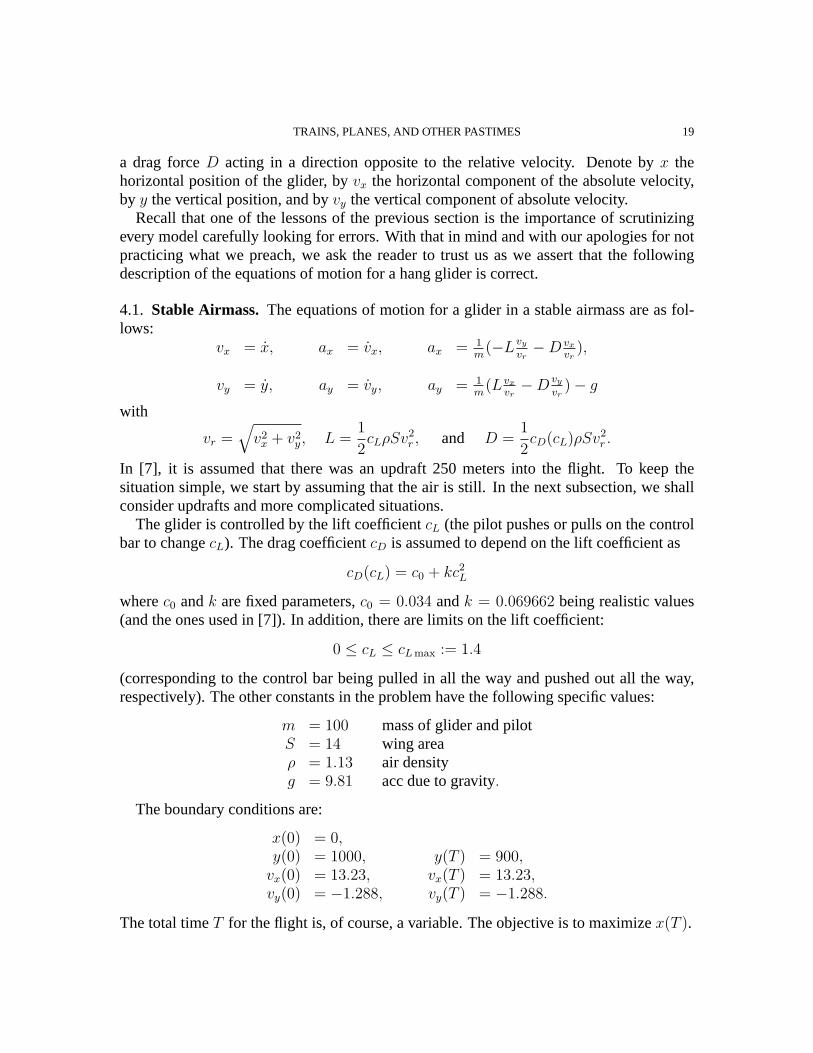
4.1. Stable Airmass. The equations of motion for a glider in a stable airmass are as fol-lows:

vx = x, ax = vx, ax = 1m

(−Lvy

vr−D vx

vr),

vy = y, ay = vy, ay = 1m

(Lvx

vr−D vy

vr)− g

with

vr =√

v2x + v2

y , L =1

2cLρSv2

r , and D =1

2cD(cL)ρSv2

r .

In [7], it is assumed that there was an updraft 250 meters into the flight. To keep thesituation simple, we start by assuming that the air is still. In the next subsection, we shallconsider updrafts and more complicated situations.

The glider is controlled by the lift coefficientcL (the pilot pushes or pulls on the controlbar to changecL). The drag coefficientcD is assumed to depend on the lift coefficient as

cD(cL) = c0 + kc2L

wherec0 andk are fixed parameters,c0 = 0.034 andk = 0.069662 being realistic values(and the ones used in [7]). In addition, there are limits on the lift coefficient:

0 ≤ cL ≤ cL max := 1.4

(corresponding to the control bar being pulled in all the way and pushed out all the way,respectively). The other constants in the problem have the following specific values:

m = 100 mass of glider and pilotS = 14 wing areaρ = 1.13 air densityg = 9.81 acc due to gravity.

The boundary conditions are:

x(0) = 0,y(0) = 1000, y(T ) = 900,

vx(0) = 13.23, vx(T ) = 13.23,vy(0) = −1.288, vy(T ) = −1.288.

The total timeT for the flight is, of course, a variable. The objective is to maximizex(T ).

20 VANDERBEI

With a stable airmass, one expects that, for appropriate choice of boundary conditions,the optimal control will be static. The optimal static control is found by minimizing theratio of drag to lift (or, equivalently, maximizingL/D):

D/L =c0

cL

+ kcL.

The minimum occurs atcL =√

c0/k = 0.69862. Then using the fact that accelerations ina static solution vanish, we deduce that

−vx

vy

=L

D= 10.274

vr =

√2mg

ρS√

c2D + c2

L

= 13.2901.

From this we quickly compute that

vx = 13.23, vy = −1.288.

That is, the initial and final velocities given above in the boundary conditions for the dy-namic version of the problem match the optimal values for the static version of the problem.Hence, we expect the optimal solution of the dynamic problem to be in fact static. Let’ssee if this is what we get.

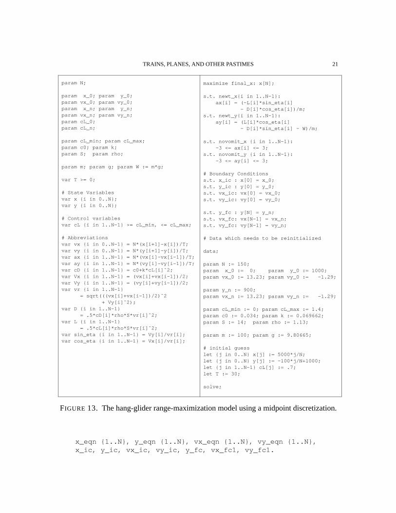
The AMPL model for the midpoint discretization is shown in Figure 13. With this dis-cretization, we have the following variables

T, x{0,..,N}, y{0,..,N}, cL{1,..,N-1}

and the following equality constraints

newt_x{i in 1..N-1}, newt_y{i in 1..N-1},x_ic, y_ic, vx_ic, vy_ic,y_fc, vx_fc, vy_fc.

Hence, with this formulation the problem involves3N+2 variables and2N+5 equality con-straints leavingN-3 degrees of freedom over which we optimize. UsingN=150, LOQO

solves this problem in 45 interior-point iterations (4.57 seconds on a 366 MHz PC). Atoptimality we havex[N]=1027.383 andT=77.6699 . The control input as a functionof time turns out to be constant as we hoped.

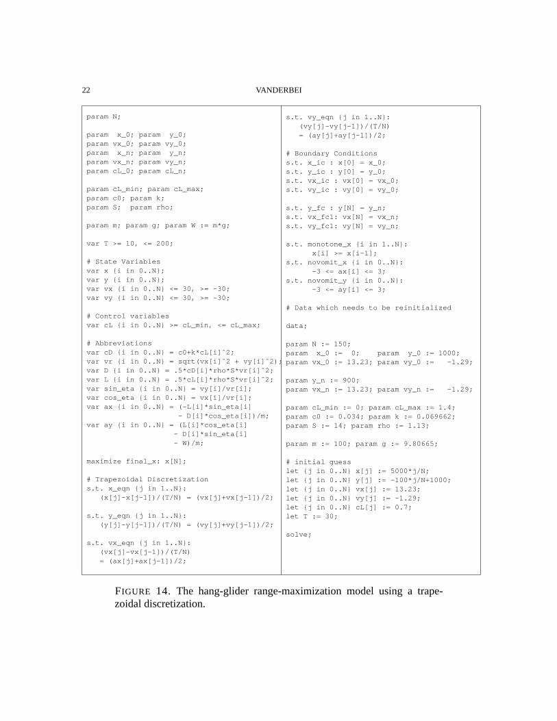
Now, let’s consider a trapezoidal discretization. TheAMPL model is shown in Figure 14.In this case, we have the following variables:

T, x{0,..,N}, y{0,..,N}, vx{0,..,N}, vy{0,..,N}, cL{0,..,N}

and the following equality constraints for the discretized problem:


param N;

param x_0; param y_0;param vx_0; param vy_0;param x_n; param y_n;param vx_n; param vy_n;param cL_0;param cL_n;

param cL_min; param cL_max;param c0; param k;param S; param rho;

param m; param g; param W := m*g;

var T >= 0;

# State Variablesvar x {i in 0..N};var y {i in 0..N};

# Control variablesvar cL {i in 1..N-1} >= cL_min, <= cL_max;

# Abbreviationsvar vx {i in 0..N-1} = N*(x[i+1]-x[i])/T;var vy {i in 0..N-1} = N*(y[i+1]-y[i])/T;var ax {i in 1..N-1} = N*(vx[i]-vx[i-1])/T;var ay {i in 1..N-1} = N*(vy[i]-vy[i-1])/T;var cD {i in 1..N-1} = c0+k*cL[i]ˆ2;var Vx {i in 1..N-1} = (vx[i]+vx[i-1])/2;var Vy {i in 1..N-1} = (vy[i]+vy[i-1])/2;var vr {i in 1..N-1}

= sqrt(((vx[i]+vx[i-1])/2)ˆ2+ Vy[i]ˆ2);

var D {i in 1..N-1}= .5*cD[i]*rho*S*vr[i]ˆ2;

var L {i in 1..N-1}= .5*cL[i]*rho*S*vr[i]ˆ2;

var sin_eta {i in 1..N-1} = Vy[i]/vr[i];var cos_eta {i in 1..N-1} = Vx[i]/vr[i];

maximize final_x: x[N];

s.t. newt_x{i in 1..N-1}:ax[i] = (-L[i]*sin_eta[i]

- D[i]*cos_eta[i])/m;s.t. newt_y{i in 1..N-1}:

ay[i] = (L[i]*cos_eta[i]- D[i]*sin_eta[i] - W)/m;

s.t. novomit_x {i in 1..N-1}:-3 <= ax[i] <= 3;

s.t. novomit_y {i in 1..N-1}:-3 <= ay[i] <= 3;

# Boundary Conditionss.t. x_ic : x[0] = x_0;s.t. y_ic : y[0] = y_0;s.t. vx_ic: vx[0] = vx_0;s.t. vy_ic: vy[0] = vy_0;

s.t. y_fc : y[N] = y_n;s.t. vx_fc: vx[N-1] = vx_n;s.t. vy_fc: vy[N-1] = vy_n;

# Data which needs to be reinitialized

data;

param N := 150;param x_0 := 0; param y_0 := 1000;param vx_0 := 13.23; param vy_0 := -1.29;

param y_n := 900;param vx_n := 13.23; param vy_n := -1.29;

param cL_min := 0; param cL_max := 1.4;param c0 := 0.034; param k := 0.069662;param S := 14; param rho := 1.13;

param m := 100; param g := 9.80665;

# initial guesslet {j in 0..N} x[j] := 5000*j/N;let {j in 0..N} y[j] := -100*j/N+1000;let {j in 1..N-1} cL[j] := .7;let T := 30;

solve;

FIGURE 13. The hang-glider range-maximization model using a midpoint discretization.

x_eqn {1..N}, y_eqn {1..N}, vx_eqn {1..N}, vy_eqn {1..N},x_ic, y_ic, vx_ic, vy_ic, y_fc, vx_fc1, vy_fc1.

22 VANDERBEI

param N;

param x_0; param y_0;param vx_0; param vy_0;param x_n; param y_n;param vx_n; param vy_n;param cL_0; param cL_n;

param cL_min; param cL_max;param c0; param k;param S; param rho;

param m; param g; param W := m*g;

var T >= 10, <= 200;

# State Variablesvar x {i in 0..N};var y {i in 0..N};var vx {i in 0..N} <= 30, >= -30;var vy {i in 0..N} <= 30, >= -30;

# Control variablesvar cL {i in 0..N} >= cL_min, <= cL_max;

# Abbreviationsvar cD {i in 0..N} = c0+k*cL[i]ˆ2;var vr {i in 0..N} = sqrt(vx[i]ˆ2 + vy[i]ˆ2);var D {i in 0..N} = .5*cD[i]*rho*S*vr[i]ˆ2;var L {i in 0..N} = .5*cL[i]*rho*S*vr[i]ˆ2;var sin_eta {i in 0..N} = vy[i]/vr[i];var cos_eta {i in 0..N} = vx[i]/vr[i];var ax {i in 0..N} = (-L[i]*sin_eta[i]

- D[i]*cos_eta[i])/m;var ay {i in 0..N} = (L[i]*cos_eta[i]

- D[i]*sin_eta[i]- W)/m;

maximize final_x: x[N];

# Trapezoidal Discretizations.t. x_eqn {j in 1..N}:

(x[j]-x[j-1])/(T/N) = (vx[j]+vx[j-1])/2;

s.t. y_eqn {j in 1..N}:(y[j]-y[j-1])/(T/N) = (vy[j]+vy[j-1])/2;

s.t. vx_eqn {j in 1..N}:(vx[j]-vx[j-1])/(T/N)= (ax[j]+ax[j-1])/2;

s.t. vy_eqn {j in 1..N}:(vy[j]-vy[j-1])/(T/N)= (ay[j]+ay[j-1])/2;

# Boundary Conditionss.t. x_ic : x[0] = x_0;s.t. y_ic : y[0] = y_0;s.t. vx_ic : vx[0] = vx_0;s.t. vy_ic : vy[0] = vy_0;

s.t. y_fc : y[N] = y_n;s.t. vx_fc1: vx[N] = vx_n;s.t. vy_fc1: vy[N] = vy_n;

s.t. monotone_x {i in 1..N}:x[i] >= x[i-1];

s.t. novomit_x {i in 0..N}:-3 <= ax[i] <= 3;

s.t. novomit_y {i in 0..N}:-3 <= ay[i] <= 3;

# Data which needs to be reinitialized

data;

param N := 150;param x_0 := 0; param y_0 := 1000;param vx_0 := 13.23; param vy_0 := -1.29;

param y_n := 900;param vx_n := 13.23; param vy_n := -1.29;

param cL_min := 0; param cL_max := 1.4;param c0 := 0.034; param k := 0.069662;param S := 14; param rho := 1.13;

param m := 100; param g := 9.80665;

# initial guesslet {j in 0..N} x[j] := 5000*j/N;let {j in 0..N} y[j] := -100*j/N+1000;let {j in 0..N} vx[j] := 13.23;let {j in 0..N} vy[j] := -1.29;let {j in 0..N} cL[j] := 0.7;let T := 30;

solve;

FIGURE 14. The hang-glider range-maximization model using a trape-zoidal discretization.


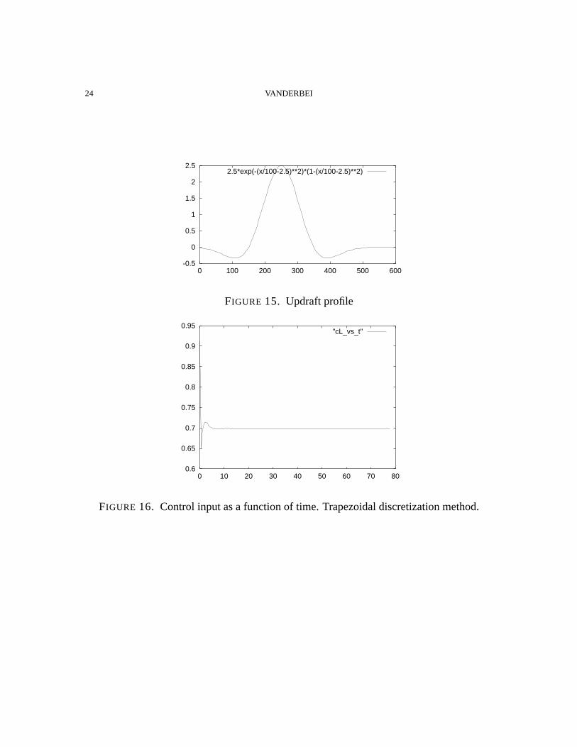
With this formulation, the problem involves5N+6 variables and4N+7 equality constraintsleavingN-1 degrees of freedom over which we optimize. This is 2 more than with theprevious model. UsingN=150, LOQO solves this problem in 141 interior-point iterations(24.2 seconds on a 366 MHz PC). At optimality we havex[N] = 1027.488 and T= 77.7241 . After flying more than a kilometer, this optimal solution is better than theprevious one by 10 centimeters. Perhaps this just reflects a difference in the discretizationor maybe it is really a different answer. To see which it is, let’s look at the control input—Figure 16. From the control input we see that this solution is definitely not static. But itis also not implementable as it is discontinuous att = 0 (followed by nontrivial controlinputs for approximately the first 9 seconds of the flight).

The discontinuity of the control input suggests that the model formulation, i.e. the dis-cretization, has too many degrees of freedom. To check this hypothesis, we tried introduc-ing continuityconstraints. First we added just one such constraint:

cL[0] = cL[1]

With this constraint, we got a solution that was closer to the static solution but was still notitself static. So, we added a second continuity constraint:

cL[1] = cL[2]

With these two constraints, the model solves in 222 interior-point iterations (41.1 secondson a 366 MHz PC). At optimality we getx[N] = 1027.383 andT = 77.6699 inexact agreement with the static solution. Furthermore, the optimal control is again static.

It is noteworthy that the “correct” number of degrees of freedom for the adjusted trape-zoidal rule matches the number of degrees of freedom from the midpoint rule. Clearly,something fundamental is going on here.

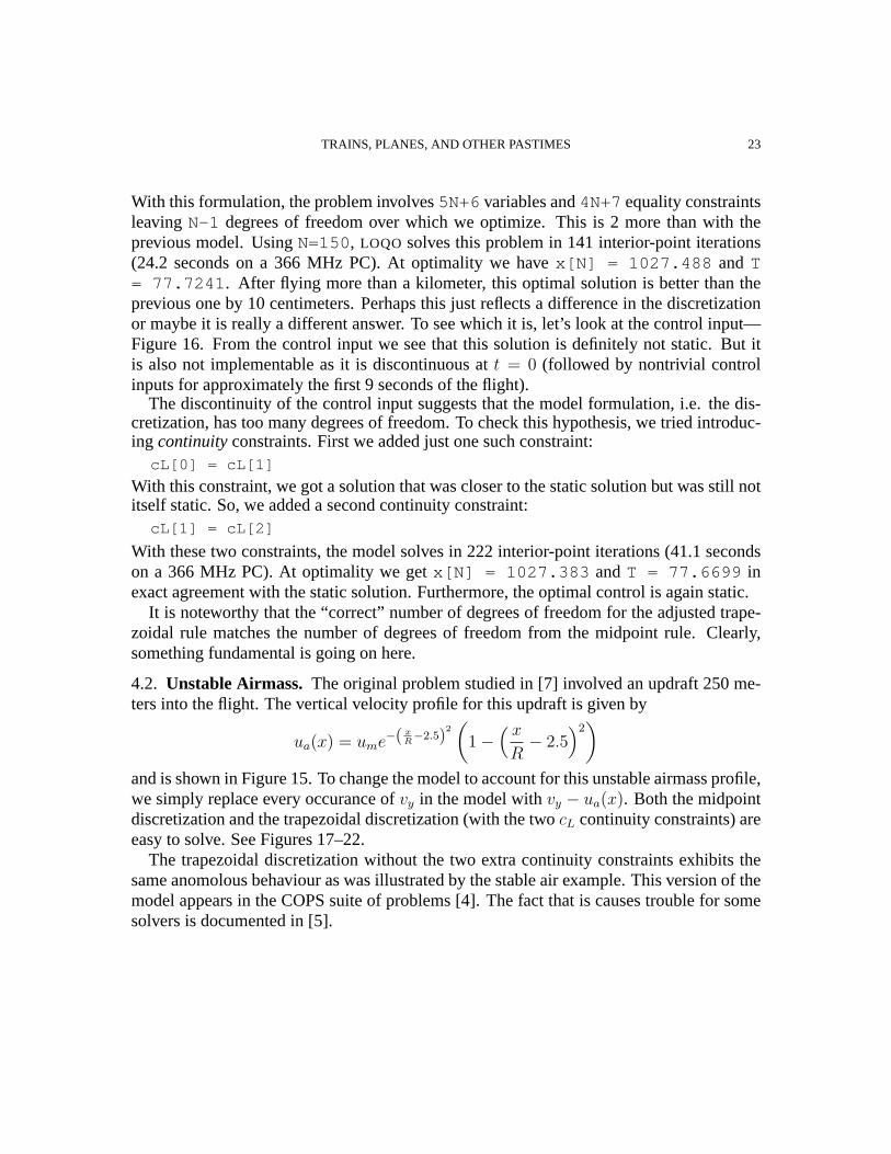
4.2. Unstable Airmass. The original problem studied in [7] involved an updraft 250 me-ters into the flight. The vertical velocity profile for this updraft is given by

ua(x) = ume−( xR−2.5)

2(

1−( x

R− 2.5

)2)

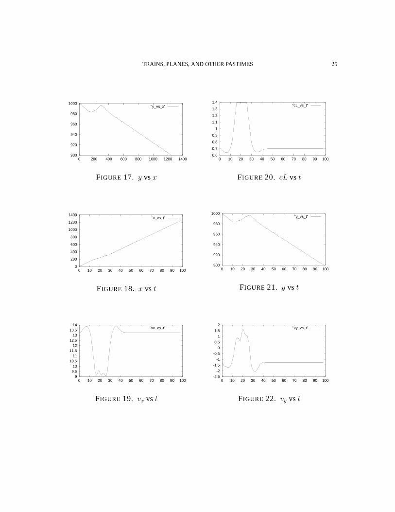
and is shown in Figure 15. To change the model to account for this unstable airmass profile,we simply replace every occurance ofvy in the model withvy − ua(x). Both the midpointdiscretization and the trapezoidal discretization (with the twocL continuity constraints) areeasy to solve. See Figures 17–22.

The trapezoidal discretization without the two extra continuity constraints exhibits thesame anomolous behaviour as was illustrated by the stable air example. This version of themodel appears in the COPS suite of problems [4]. The fact that is causes trouble for somesolvers is documented in [5].

24 VANDERBEI

-0.5

0

0.5

1

1.5

2

2.5

0 100 200 300 400 500 600

2.5*exp(-(x/100-2.5)**2)*(1-(x/100-2.5)**2)

FIGURE 15. Updraft profile

0.6

0.65

0.7

0.75

0.8

0.85

0.9

0.95

0 10 20 30 40 50 60 70 80

"cL_vs_t"

FIGURE 16. Control input as a function of time. Trapezoidal discretization method.


900

920

940

960

980

1000

0 200 400 600 800 1000 1200 1400

"y_vs_x"

FIGURE 17. y vsx

0

200

400

600

800

1000

1200

1400

0 10 20 30 40 50 60 70 80 90 100

"x_vs_t"

FIGURE 18. x vs t

99.510

10.511

11.512

12.513

13.514

0 10 20 30 40 50 60 70 80 90 100

"vx_vs_t"

FIGURE 19. vx vs t

0.6

0.7

0.8

0.9

1

1.1

1.2

1.3

1.4

0 10 20 30 40 50 60 70 80 90 100

"cL_vs_t"

FIGURE 20. cL vs t

900

920

940

960

980

1000

0 10 20 30 40 50 60 70 80 90 100

"y_vs_t"

FIGURE 21. y vs t

-2.5

-2

-1.5

-1

-0.5

0

0.5

1

1.5

2

0 10 20 30 40 50 60 70 80 90 100

"vy_vs_t"

FIGURE 22. vy vs t

26 VANDERBEI

For more on optimal control of flight paths, we refer the reader to Stengel’s classic text[12] and to the recent book by Bryson [6].

4.3. Lessons.In this section there are two lessons:

(1) Before solving a problem of interest, always test a model by first solving a problemwhose solution is mathematically tractible.

(2) The two discretization methods that we’ve discussed throughout this paper are com-monly used for simple numerical integration of ODEs. In this case, the problem iswell-posed if the number of equations matches the number of variables; i.e., thereare no degrees of freedom. One can show that a problem is well-posed with respectto midpoint discretization if and only if it is well-posed with respect to trapezoidaldiscretization. However, as we saw in this example, for control problems, i.e. prob-lems where there are degrees of freedom, the midpoint discretization will some-times have fewer degrees of freedom than the trapezoidal discretization. It seemsthat the midpoint discretization has the “correct” number and that the trapezoidaldiscretization has too many.

5. TOBOGGANING

It wouldn’t be right to end our discussion of trajectory optimization without discussingthe famous Brachistochrone problem. We do it here in this last section in the context ofdesigning a slide which will get the rider from the beginning to the end in the shortestamount of time.

We assume in this study that the slide will be constructed out of frictionless material. Welet x denote, as usual, horizontal displacement and we lety denote vertical displacement.In contrast with earlier conventions, we assume thaty increases as one moves downward.The slide will connect two points having coordinates(x0, y0) = (0, 0) and(xf , yf ). Thetoboggan starts from rest at the top of the slide. Hence, initially the toboggan has zerokinetic energy and zero potential energy (due to gravity). Since the slide is frictionless,there is no loss of energy as heat. By conservation of energy, the total energy must alwaysremain zero. So, when the toboggan has dropped to levely, we have

1

2mv2 −mgy = 0.

Here,v denotes the speed of the toboggan. From this relation we see that

v =√

2gy.

Now, the time to do the run can be computed as an integral of differential chunks of time

T =

∫ T

0

dt =

∫ T

0

ds(t)

v(t).


param n := 512;

param x {j in 0..n} := j/n;

# Variablesvar y {j in 0..n} >= 0;

# Abbreviationsvar dydx {j in 1..n}

= (y[j]-y[j-1])/(x[j]-x[j-1]);var f {j in 1..n}

= sqrt( (1+dydx[j]ˆ2)/y[j-1] );

minimize time:sum {j in 1..n}

f[j]*(x[j]-x[j-1]) ;

subject to y0: y[0] = 1.0e-12;subject to yn: y[n] = 1;

subject to monotone {j in 1..n}:dydx[j] >= 0;

let {j in 0..n} y[j] := x[j];

solve;

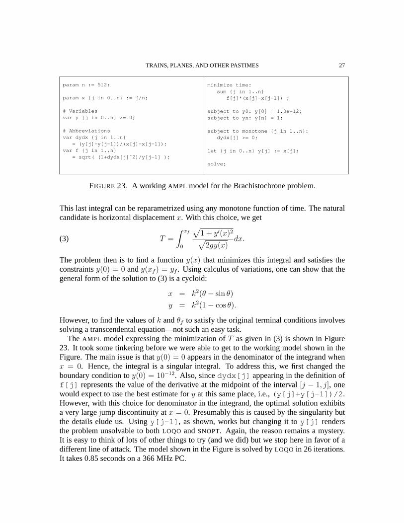
FIGURE 23. A workingAMPL model for the Brachistochrone problem.

This last integral can be reparametrized using any monotone function of time. The naturalcandidate is horizontal displacementx. With this choice, we get

(3) T =

∫ xf

0

√1 + y′(x)2√

2gy(x)dx.

The problem then is to find a functiony(x) that minimizes this integral and satisfies theconstraintsy(0) = 0 andy(xf ) = yf . Using calculus of variations, one can show that thegeneral form of the solution to (3) is a cycloid:

x = k2(θ − sin θ)

y = k2(1− cos θ).

However, to find the values ofk andθf to satisfy the original terminal conditions involvessolving a transcendental equation—not such an easy task.

The AMPL model expressing the minimization ofT as given in (3) is shown in Figure23. It took some tinkering before we were able to get to the working model shown in theFigure. The main issue is thaty(0) = 0 appears in the denominator of the integrand whenx = 0. Hence, the integral is a singular integral. To address this, we first changed theboundary condition toy(0) = 10−12. Also, sincedydx[j] appearing in the definition off[j] represents the value of the derivative at the midpoint of the interval[j − 1, j], onewould expect to use the best estimate fory at this same place, i.e.,(y[j]+y[j-1])/2 .However, with this choice for denominator in the integrand, the optimal solution exhibitsa very large jump discontinuity atx = 0. Presumably this is caused by the singularity butthe details elude us. Usingy[j-1] , as shown, works but changing it toy[j] rendersthe problem unsolvable to bothLOQO andSNOPT. Again, the reason remains a mystery.It is easy to think of lots of other things to try (and we did) but we stop here in favor of adifferent line of attack. The model shown in the Figure is solved byLOQO in 26 iterations.It takes 0.85 seconds on a 366 MHz PC.

28 VANDERBEI

param n := 512;

param y {j in 0..n} := (j/n);

# Variablesvar x {j in 0..n};

# Abbreviationsvar dxdy {j in 1..n}

= (x[j] - x[j-1])/(y[j] - y[j-1]);var f {j in 1..n}

= sqrt( (dxdy[j]ˆ2+1)/((y[j]+y[j-1])/2) );

minimize time:sum {j in 1..n} f[j]*(y[j]-y[j-1]) ;

subject to x0: x[0] = 0;subject to xn: x[n] = 1;

let {j in 0..n} x[j] := y[j];

solve;

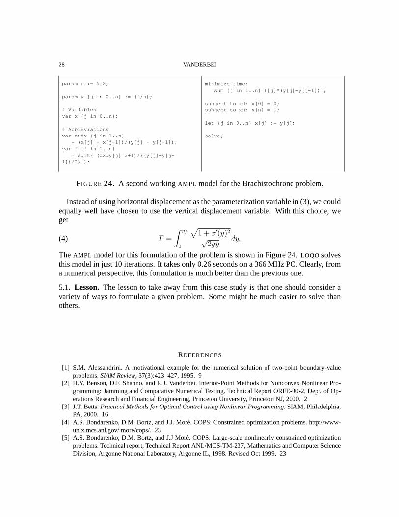
FIGURE 24. A second workingAMPL model for the Brachistochrone problem.

Instead of using horizontal displacement as the parameterization variable in (3), we couldequally well have chosen to use the vertical displacement variable. With this choice, weget

(4) T =

∫ yf

0

√1 + x′(y)2

√2gy

dy.

The AMPL model for this formulation of the problem is shown in Figure 24.LOQO solvesthis model in just 10 iterations. It takes only 0.26 seconds on a 366 MHz PC. Clearly, froma numerical perspective, this formulation is much better than the previous one.

5.1. Lesson. The lesson to take away from this case study is that one should consider avariety of ways to formulate a given problem. Some might be much easier to solve thanothers.

REFERENCES

[1] S.M. Alessandrini. A motivational example for the numerical solution of two-point boundary-valueproblems.SIAM Review, 37(3):423–427, 1995. 9

[2] H.Y. Benson, D.F. Shanno, and R.J. Vanderbei. Interior-Point Methods for Nonconvex Nonlinear Pro-gramming: Jamming and Comparative Numerical Testing. Technical Report ORFE-00-2, Dept. of Op-erations Research and Financial Engineering, Princeton University, Princeton NJ, 2000. 2

[3] J.T. Betts.Practical Methods for Optimal Control using Nonlinear Programming. SIAM, Philadelphia,PA, 2000. 16

[4] A.S. Bondarenko, D.M. Bortz, and J.J. More. COPS: Constrained optimization problems. http://www-unix.mcs.anl.gov/ more/cops/. 23

[5] A.S. Bondarenko, D.M. Bortz, and J.J More. COPS: Large-scale nonlinearly constrained optimizationproblems. Technical report, Technical Report ANL/MCS-TM-237, Mathematics and Computer ScienceDivision, Argonne National Laboratory, Argonne IL, 1998. Revised Oct 1999. 23

http://www.sor.princeton.edu/~rvdb/ps/loqo3_3.pdf

http://www.sor.princeton.edu/~rvdb/ps/loqo3_3.pdf

http://www-unix.mcs.anl.gov/~more/cops/





[6] A.E. Bryson.Dynamic Optimization. Addison Wesley Longman, Inc., Menlo Park, CA, 1999. 26[7] R. Bulirsch, E. Nerz, H.J. Pesch, and O. von Stryk. Combining direct and indirect methods in optimal

control: Range maximization of a hang glider. In R. Bulirsch, A. Miele, J. Stoer, and K.H. Well, editors,”Optimal Control: Calculus of Variations, Optimal Control Theory and Numerical Methods, pages273–288. Birkhauser Verlag, Basel, Boston, Berlin, 1993. 18, 19, 23

[8] A.R. Conn, N. Gould, and Ph.L. Toint. Constrained and unconstrained testing environment.http://www.dci.clrc.ac.uk/Activity.asp?CUTE. 9

[9] R. Fourer, D.M. Gay, and B.W. Kernighan.AMPL: A Modeling Language for Mathematical Program-ming. Scientific Press, 1993. 2

[10] P.E. Gill, W. Murray, and M.A. Saunders. User’s guide for SNOPT 5.3: A Fortran package for large-scale nonlinear programming. Technical report, Systems Optimization Laboratory, Stanford University,Stanford, CA, 1997. 2

[11] J. Kautsky and N.K. Nichols. OTEP-2: Optimal train energy programme, mark 2. Technical ReportNumerical Analysis Report NA/4/83, Dept. of Mathematics, University of Reading, 1983. 9

[12] R.F. Stengel.Optimal Control and Estimation. Dover, Mineola, NY, 1994. 26[13] R.J. Vanderbei. LOQO: An interior point code for quadratic programming.Optimization Methods and

Software, 12:451–484, 1999. 2[14] R.J. Vanderbei. LOQO user’s manual—version 3.10.Optimization Methods and Software, 12:485–514,

1999. 2[15] R.J. Vanderbei and D.F. Shanno. An interior-point algorithm for nonconvex nonlinear programming.

Computational Optimization and Applications, 13:231–252, 1999. 2

ROBERT J. VANDERBEI, PRINCETON UNIVERSITY, PRINCETON, NJ

http://www.dci.clrc.ac.uk/Activity.asp?CUTE

case studies in trajectory optimization: trains, …rvdb/tex/trajopt/trajopt.pdfcase studies in...

Documents