carbon sequestration potential of agroforestry...
TRANSCRIPT
1
CARBON SEQUESTRATION POTENTIAL OF AGROFORESTRY SYSTEMS
IN THE WEST AFRICAN SAHEL:
AN ASSESSMENT OF BIOLOGICAL AND SOCIOECONOMIC FEASIBILITY
By
ASAKO TAKIMOTO
A DISSERTATION PRESENTED TO THE GRADUATE SCHOOL
OF THE UNIVERSITY OF FLORIDA IN PARTIAL FULFILLMENT
OF THE REQUIREMENTS FOR THE DEGREE OF
DOCTOR OF PHILOSOPHY
UNIVERSITY OF FLORIDA
2007
2
©2007 Asako Takimoto

3
To my parents and grandmother
4
ACKNOWLEDGMENTS
I am indebted and grateful for many individuals and organizations who contributed to this
study and my doctoral program. I thank my chair, Dr. P.K. Nair, for his dedication and guidance
throughout this process, and my committee, Dr. Nick Comerford, Dr. Janaki Alavalapati, Dr.
Tim Martin, Dr. Ted Schuur, and Dr. V.D. Nair, for their support and encouragement.
I recognize and express my sincere gratitude to the individuals and their institutions that
supported me during my doctoral studies: the School of Forest Resources and Conservation
(Cherie Arias, Sherry Tucker, Dr. Tim White), University of Florida International Center (Debby
Anderson), the Center for Tropical Conservation and Development of UF, the World
Agroforestry Centre (especially Dr. Bocary Kaya), the Fulbright Program, and the Joint
Japan/World Bank Graduate Scholarship Program (JJ/WBGSP).
At the fieldwork in Ségou, Mali, I received tremendous support and cooperation from the
farmers, field officers, and other collaborators. It was one of the most challenging times of my
life, and I could not go through without them. Thank you to Nicole Demers, Bayo Mounkoro,
Keita, Samake, and other officers in ICRAF Ségou office, Kayo Sakaguchi, Takako Uchida, Mr.
Kiyoshi Sakai, and all the farmers in Ségou who let me use their fields for data collections and
participated the survey.
I have greatly benefited from my friendship with colleagues in the agroforestry lab at UF.
I thank Solomon Haile, Alyson Dagang, Julie Clingerman, Sam Allen, Eddie Ellis, Brian Becker,
Joyce Leptu, David Howlett, Wendy Francesconi, Subrajit Saha, Shinjiro Sato, and Masaaki
Yamada, for the discussions and supports.
To my precious friends who have been an integral part of the many years of this process,
thank you Gogce Kayihan, Brian Daley, Elli Sugita, Mike Bannister, Jason and Karen Hupp,

5
Charlotte Skov, Chrysa Mitraki, Rania Habib, Maitreyi Mandal, Trina Hofreiter, Troy Thomas,
and my fiancé, Nick Georgelis.
Last but not least, I express my most profound gratitude to my mother Ayuko Takimoto,
whose endless love and confidence in me made me come this far.
6
TABLE OF CONTENTS
page
ACKNOWLEDGMENTS ...............................................................................................................4
LIST OF TABLES .........................................................................................................................10
LIST OF FIGURES .......................................................................................................................11
ABSTRACT ...................................................................................................................................13
CHAPTER
1 INTRODUCTION ..................................................................................................................15
Background .............................................................................................................................15
Rationale and Significance .....................................................................................................16
Research Questions and Objectives ........................................................................................17
Dissertation Overview ............................................................................................................18
2 THE WEST AFRICAN SAHEL: GENERAL LAND-USE AND AGROFORESTRY ........20
Description of the Region .......................................................................................................20
Climate ............................................................................................................................20
Vegetation ........................................................................................................................21
Soil ...................................................................................................................................22
Traditional Farming Systems and Agroforestry in the WAS .................................................24
Traditional Agroforestry Practices ..................................................................................25
Bush fallow/shifting cultivation ...............................................................................25
Parkland system ........................................................................................................25
Improved Agroforestry Practices ....................................................................................26
3 LITERATURE REVIEW: CARBON SEQUESTRATION POTENTIAL OF
AGROFORESTRY SYSTEMS IN THE WEST AFRICAN SAHEL (WAS) .......................36
Overview .................................................................................................................................36
C Sequestration as a Climate-Change-Mitigation Activity .............................................36
Agroforestry for C sequestration .....................................................................................37
Methodologies for C Sequestration Measurements ................................................................39
Direct On-site Measurement ............................................................................................39
Inventory ..................................................................................................................40
Conversion and estimation .......................................................................................40
Indirect Remote Sensing Techniques ..............................................................................42
Modeling ..........................................................................................................................43
Default Values for Land/Activity Based Practices ..........................................................44
Accounting Methods ...............................................................................................................44
7
Approaches to Assessing C Sequestration Performance .................................................45
Fluxes of C and flow summation .............................................................................45
Average changes in the stocks of C .........................................................................45
Cumulative C storage ...............................................................................................46
Other accounting methods ........................................................................................46
Technical Problems and Uncertainties ............................................................................47
Biomass C Sequestration ........................................................................................................48
Studies in Various Ecoregions .........................................................................................48
Studies in West Africa .....................................................................................................48
Soil C Sequestration ...............................................................................................................50
Studies of Soil C Stock and Dynamics ............................................................................50
Soil C in the WAS ...........................................................................................................52
Socioeconomic Implications ...................................................................................................54
Economic Models ............................................................................................................54
National/global scale ................................................................................................54
Micro/site-specific scale ...........................................................................................55
Feasibility in West Africa ................................................................................................56
4 ABOVEGROUND AND BELOWGROUND CARBON STOCKS IN TRADITIONAL
AND IMPROVED AGROFORESTRY SYSTEMS IN MALI, WEST AFRICA .................61
Introduction .............................................................................................................................61
Materials and Methods ...........................................................................................................62
Study Area .......................................................................................................................62
Republic of Mali .......................................................................................................63
Ségou region .............................................................................................................63
Selected Land-use Systems for Field Data Collection ....................................................64
Parkland systems ......................................................................................................64
Improved agroforestry systems ................................................................................65
Abandoned (degraded) land .....................................................................................66
Research Design ..............................................................................................................66
Data Collection ................................................................................................................67
Biomass measurement ..............................................................................................67
Soil sampling ............................................................................................................68
Carbon Stock Estimation .................................................................................................68
Biomass C stock .......................................................................................................69
Soil C stock ..............................................................................................................71
Statistical Analysis ..........................................................................................................71
Results.....................................................................................................................................72
C Stock in Biomass and Soil ...........................................................................................72
Total C Stock ...................................................................................................................72
Relationship between Biomass C and Soil C ..................................................................73
Discussion ...............................................................................................................................73
8
5 SOIL CARBON SEQUESTRATION IN DIFFERENT PARTICLE-SIZE FRACTIONS
AT VARYING DEPTHS UNDER AGROFORESTRY SYSTEMS IN MALI ....................83
Introduction .............................................................................................................................83
Research Questions .................................................................................................................85
Materials and Methods ...........................................................................................................85
Research Design ..............................................................................................................86
Soil Preparation and Analyses .........................................................................................87
Soil fractionation ......................................................................................................87
C isotopic ratio (13
C/12
C) measurement ...................................................................88
Statistical Analysis ..........................................................................................................89
Results.....................................................................................................................................90
Soil Characteristics ..........................................................................................................90
Whole Soil C ...................................................................................................................91
C in Soil Fractions ...........................................................................................................92
Isotope Analysis of Whole Soil C ...................................................................................93
Isotope Analysis of C in Soil Fractions ...........................................................................94
Relationships of Data Sets ...............................................................................................94
Discussion ...............................................................................................................................95
6 SOCIOECONOMIC ANALYSIS OF THE CARBON SEQUESTRATION
POTENTIAL OF IMPROVED AGROFORESTRY SYSTEMS IN MALI, WEST
AFRICA ................................................................................................................................117
Introduction ...........................................................................................................................117
Research Questions ...............................................................................................................118
Materials and Methods .........................................................................................................119
Social Survey of Fodder Bank Farmers .........................................................................119
Local Market Survey .....................................................................................................120
Types of Analysis ..........................................................................................................121
Cost-benefit analysis (CBA) ..................................................................................121
Sensitivity analysis .................................................................................................127
Risk modeling ........................................................................................................128
Results...................................................................................................................................129
Demographic Characteristics of Target Population ......................................................129
Cost-Benefit Analysis: Best Guess Scenario of the Live Fence and the Fodder Bank .130
Sensitivity Analysis .......................................................................................................132
Risk Modeling and Simulation ......................................................................................132
Discussion .............................................................................................................................134
7 SUMMARY AND CONCLUSIONS ...................................................................................148
C Sequestration Potential ......................................................................................................148
Biophysical Potential .....................................................................................................148
Socioecomic Potential ...................................................................................................150
Conclusions ...................................................................................................................152
9
Agroforestry Adoption for C sequestration in the Study Region .........................................152
Limiting Factors ............................................................................................................152
Favorable Factors ..........................................................................................................153
Implications for Agroforestry ...............................................................................................154
Future Research ....................................................................................................................155
APPENDIX
A SOCIAL SURVEY QUESTIONNAIRE FOR FODDER BANK OWNERS ......................156
B COST BENEFIT ANALYSIS (CASH FLOW) OF LIVE FENCE .....................................163
C COST BENEFIT ANALYSIS (CASH FLOW) OF FODDER BANK ................................167
LIST OF REFERENCES .............................................................................................................171
BIOGRAPHICAL SKETCH .......................................................................................................184
10
LIST OF TABLES
Table page
2-1 Common tree and shrub species found throughout the West African Sahel .....................29
2-2 Main productive functions of agroforestry parklands ........................................................31
3-1 Summary of various biomass C measurement approaches used commonly in C
sequestration studies ..........................................................................................................59
3-2 Aboveground time-averaged C stock in different ecosystems and agroforestry
practices .............................................................................................................................60
4-1 Characteristics of the villages where the experimental plots were set up in Ségou
region, Mali ........................................................................................................................76
4-2 Characteristics of the experimental plots (three plots average) for five-selected land-
use systems in Ségou region, Mali .....................................................................................76
4-3 Estimated biomass C (above and below ground) stock values of each plot and three
plots average of five selected land-use systems .................................................................77
4-4 Total C stock (biomass C + soil C of different depth) of five selected land-use
systems. ..............................................................................................................................77
5-1 Soil profile characteristics for plots of the five land-use systems used in the study at
Ségou Region, Mali .........................................................................................................101
5-2 δ13
C values of whole soil and three fraction sizes from five studied land-use systems,
at Ségou Region, Mali......................................................................................................102
6-1 Demographic characteristics of the target population in Ségou, Mali .............................138
6-2 Net Present Value (NPV), Benefit Cost Ratio (BCR), and Internal Rate of Return
(IRR) of the live fence and the fodder bank projects in the three different scenarios
(without C sale, with C sale by the ideal accounting method, and with C sale by the
tonne-year accounting method) in Ségou, Mali ...............................................................138
6-3 NPV sensitivity of the live fence project and the fodder bank project to the change of
an input variable in Ségou, Mali ......................................................................................139
11
LIST OF FIGURES
Figure page
2-1 Map of West Africa with ecological zones and isohyetal lines .........................................32
2-2 Standardized annual Sahel rainfall (June to October) from 1898 to 2004 .........................33
2-3 Seasonal landscape contrast of the WAS ...........................................................................33
2-4 Distribution of soil orders (USDA soil taxonomy) in West Africa ...................................34
2-5 Parkland system in Ségou, Mali.........................................................................................35
2-6 Allowing the cattle to roam freely on the landscape during the dry season ......................35
4-1 Location map of A: Mali; B: Mali showing its land-locked nature: C: Map of
Ségou region ......................................................................................................................78
4-2 Faidherbia albida parkland in Togo village ......................................................................79
4-3 Vitellaria paradoxa parkland in Dakala village.................................................................79
4-4 Live fence system in Dougoukouna village .......................................................................80
4-5 Fodder bank in Dakala village ...........................................................................................80
4-6 Abandoned land just outside of Diamaribougou village....................................................81
4-7 Aboveground and belowground C stock per ha of five selected land-use systems ...........82
5-1 Soil sampling, Ségou, Mali ..............................................................................................103
5-2 Soil pits dug in plots of the five land-use systems studied in Ségou region of Mali .......104
5-3 Model of soil organic matter dynamics ...........................................................................105
5-4 Whole soil C content of three depth classes (0 – 10 cm, 10 – 40 cm, and 40 – 100
cm) in different land-use systems in Ségou, Mali ............................................................106
5-5 Soil C content of three particle size fractions in three depth classes (0 – 10 cm, 10 –
40 cm, and 40 – 100 cm) under five land-use systems in Ségou, Mali ...........................107
5-6 Whole soil C, divided into C3 plants (trees)- origin and C4 plants (crops)-origin, in
different soil layers up to 100 cm depth, in five land-use systems in Ségou, Mali .........108
5-7 Soil C in three fraction sizes divided into C3 plants-origin and C4 plants-origin in
different soil particle-size fractions under different land-use systems in Ségou, Mali ....109
12
5-8 Linear regression between silt + clay content of soil and whole soil C content in three
depth classes across five land-use systems in Ségou region of Mali ...............................112
5-9 Linear regression between silt and clay content of soil and C in soil particles of <53
μm in three soil-depth classes across five land-use systems in Ségou, Mali ...................114
5-10 Linear regression between C derived from C3 plants and C in the large soil particles
(250 – 2000 μm) at 0 – 10 cm soil depth across five land-use systems of Ségou
region, Mali. .....................................................................................................................116
6-1 Social survey with farmers in Ségou, Mali ......................................................................140
6-2 Simulated NPV probability distribution of the live fence project (without C sale).........140
6-3 Simulated net benefit (total costs – total revenues in each year) of the live fence
project (without C sale) ....................................................................................................141
6-4 Simulated NPV probability distribution of the live fence project (with C sale by the
ideal accounting method) .................................................................................................142
6-5 Regression sensitivity analysis for NPV of the live fence project (with C sale by the
ideal accounting method) .................................................................................................143
6-6 Simulated NPV probability distribution of the fodder bank project (without C sale) .....144
6-7 Simulated net benefit (total costs – total revenues in each year) of the fodder bank
project (without C sale) ....................................................................................................145
6-8 Simulated NPV probability distribution of the fodder bank project (with C sale by
the ideal accounting method) ...........................................................................................146
6-9 Regression sensitivity analysis for NPV of the fodder bank project (with C sale by
the ideal accounting method) ...........................................................................................147
13
Abstract of Dissertation Presented to the Graduate School
of the University of Florida in Partial Fulfillment of the
Requirements for the Degree of Doctor of Philosophy
CARBON SEQUESTRATION POTENTIAL OF AGROFORESTRY SYSTEMS
IN THE WEST AFRICAN SAHEL:
AN ASSESSMENT OF BIOLOGICAL AND SOCIOECONOMIC FEASIBILITY
By
Asako Takimoto
December 2007
Chair: P. K. Ramachandran Nair
Major: Forest Resources and Conservation
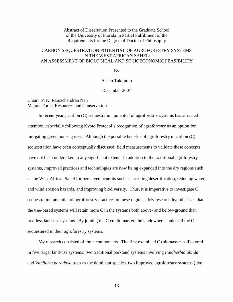
In recent years, carbon (C) sequestration potential of agroforestry systems has attracted
attention, especially following Kyoto Protocol‘s recognition of agroforestry as an option for
mitigating green house gasses. Although the possible benefits of agroforestry in carbon (C)
sequestration have been conceptually discussed, field measurements to validate these concepts
have not been undertaken to any significant extent. In addition to the traditional agroforestry
systems, improved practices and technologies are now being expanded into the dry regions such
as the West African Sahel for perceived benefits such as arresting desertification, reducing water
and wind erosion hazards, and improving biodiversity. Thus, it is imperative to investigate C
sequestration potential of agroforestry practices in these regions. My research hypothesizes that
the tree-based systems will retain more C in the systems both above- and below-ground than
tree-less land-use systems. By joining the C credit market, the landowners could sell the C
sequestered in their agroforestry systems.
My research consisted of three components. The first examined C (biomass + soil) stored
in five target land-use systems: two traditional parkland systems involving Faidherbia albida
and Vitellaria paradoxa trees as the dominant species, two improved agroforestry systems (live
14
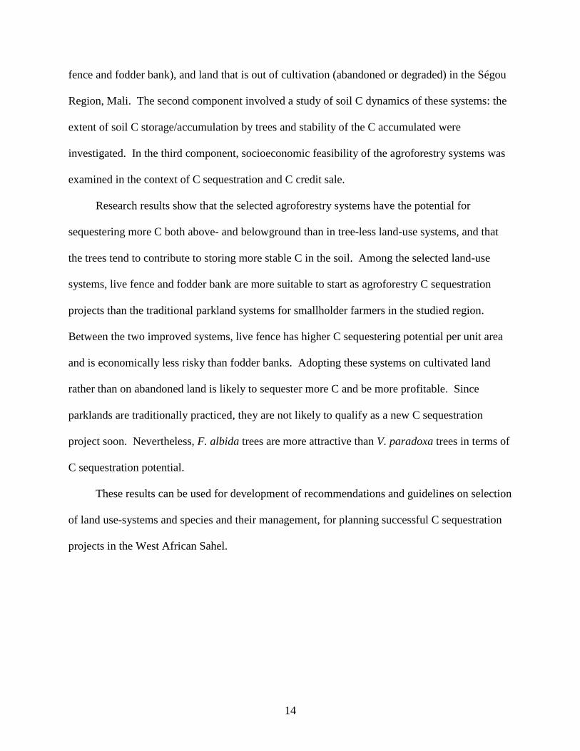
fence and fodder bank), and land that is out of cultivation (abandoned or degraded) in the Ségou
Region, Mali. The second component involved a study of soil C dynamics of these systems: the
extent of soil C storage/accumulation by trees and stability of the C accumulated were
investigated. In the third component, socioeconomic feasibility of the agroforestry systems was
examined in the context of C sequestration and C credit sale.
Research results show that the selected agroforestry systems have the potential for
sequestering more C both above- and belowground than in tree-less land-use systems, and that
the trees tend to contribute to storing more stable C in the soil. Among the selected land-use
systems, live fence and fodder bank are more suitable to start as agroforestry C sequestration
projects than the traditional parkland systems for smallholder farmers in the studied region.
Between the two improved systems, live fence has higher C sequestering potential per unit area
and is economically less risky than fodder banks. Adopting these systems on cultivated land
rather than on abandoned land is likely to sequester more C and be more profitable. Since
parklands are traditionally practiced, they are not likely to qualify as a new C sequestration
project soon. Nevertheless, F. albida trees are more attractive than V. paradoxa trees in terms of
C sequestration potential.
These results can be used for development of recommendations and guidelines on selection
of land use-systems and species and their management, for planning successful C sequestration
projects in the West African Sahel.
15
CHAPTER 1
INTRODUCTION
Background
It is widely accepted that current global climate change or global warming is ―the‖ most
serious environmental issue affecting human lives. Global warming refers to the increase in the
average temperature of the Earth's near-surface air and oceans in recent decades and its projected
continuation. It is brought about primarily by the increase in atmospheric concentrations of the
so-called greenhouse gases (GHGs). GHGs are components of atmosphere contributing to the
―green house effect,‖ the process in which the emission of infrared radiation by the atmosphere
warms a planet‘s surface. The Intergovernmental Panel on Climate Change (IPCC), established
by the United Nations (UN) to evaluate the risk of climate change concludes in its most recent
report that ―most of the observed increase in globally averaged temperatures since the mid-20th
century is very likely due to the observed increase in anthropogenic greenhouse gas
concentrations‖ (IPCC 2007). The Kyoto Protocol to the United Nations Framework Convention
on Climate Change (UNFCC) is the first and so far the largest international agreement to
stabilize GHG concentrations
Carbon dioxide (CO2) is a major GHG and its concentration build-up is accelerated by
human activities such as burning of fossil fuels and deforestation. One of the approaches to
reducing CO2 concentration in the atmosphere, called biomass carbon (C) sequestration, is to
―store‖ it in forest and forest soils by trees and other plants through photosynthesis. This concept
became widely known because the Kyoto Protocol has an approach called Land Use, Land Use
Change and Forestry (LULUCF), which allows the use of C sequestration through afforestation
and reforestation as a form of GHG offset activities. The Marrakesh Accords in 2001
determined more detailed rules of LULUCF and added forest management, crop management,
16
grazing land management, and revegetation as LULUCF activities. This enables agroforestry to
be an activity of C sequestration under the Kyoto Protocol, and since then, C sequestration
potential of agroforestry systems has attracted attention from both industrialized and developing
countries (Albrecht and Kandji 2003; Makundi and Sathaye 2004; Sharrow and Ismail 2004).
This became particularly relevant because of an arrangement called Clean Development
Mechanism (CDM) under the Kyoto Protocol, which allows industrialized countries with a
GHGs reduction commitment to invest in mitigation projects in developing countries as an
alternative to what is generally more costly in their own countries. Since agroforestry is mostly
practiced by subsistence farmers in developing countries, there is an attractive opportunity for
those farmers to benefit economically from agroforestry if the C sequestered through
agroforestry activities are sold to developed countries; it will be an environmental benefit to the
global community at large as well.
Rationale and Significance
The IPCC Report (2000) estimates that 630 million ha of unproductive croplands and
grasslands could be converted to agroforestry worldwide, with the potential to sequester 0.391
Pg of C (1 Pg = petagram = 1015
g = 1 billion ton) per year by 2010 and 0.586 Pg C per year by
2040. The credibility of conceptual models and theoretical foundations of the possible benefits
of agroforestry in C sequestration have been suggested: agroforestry has C storage potential in its
multiple plant species and soil, high applicability in agricultural land, and indirect effects such as
decreasing pressure on natural forest or soil erosion (Nair and Nair 2003; Lal 2004a; Montagnini
and Nair 2004). Field measurements to validate these concepts and hypotheses, however, have
not been undertaken to a significant extent. Some studies of specific agroforestry practices
proved the potential of C sequestration and its benefits, such as the Indonesian homegarden
systems (Roshetko et al. 2002; Schroth et al. 2002). But very few such studies have been
17
reported regarding C sequestration potential of agroforestry systems in semiarid and arid regions.
In addition to already existing indigenous agroforestry systems, improved practices and
technologies are now being expanded into these dry regions for perceived benefits such as
arresting desertification, reducing water and wind erosion hazards, and improving biodiversity
(Droppelmann et al. 2000; Gordon et al. 2003). In this scenario, it is imperative that C
sequestration potential of agroforestry practices in these regions is investigated. Considering that
the ecological production potential of these dry ecosystems is inherently low compared to that of
―high-potential‖ areas of better climatic and soil conditions, the extent to which agroforestry
systems can contribute – if at all – to C sequestration in such regions is in itself an important
issue.
This study was conducted in Mali, situated in the West African Sahel (WAS), one of the
largest semiarid regions of the world. Considering the large extent of area of the region (approx.
5.4 million km2), results of studies of this nature are likely to have wide applicability; yet, such
studies have been rare, possibly because of the relative backwardness of the region in terms of
economic development and therefore research facilities and infrastructure. Needless to say, such
studies are important because of their relevance in the context of C credit sale under CDM. The
WAS is one of the most environmentally vulnerable and poorest areas in the world. If the
majority of the people who are subsistence farmers can receive even small amounts of C
payments through their agroforestry practices, it would be a substantial contribution to their
economic welfare and the overall development of the region. Thus, an analysis of the C
sequestration potential of various agroforestry practices (traditional and newly introduced) in the
region is timely.
Research Questions and Objectives
To address the issues discussed above, four research questions are raised:
18
1. How much C is stored in different agroforestry systems aboveground and belowground?
2. How do trees contribute to C storage in the soil, and how labile is this C?
3. What is the overall relative attractiveness of each of the selected agroforestry systems
considering its C sequestration potential in the context of its biological potential, economic
profitability, and social acceptability?
4. If carbon credit markets were introduced under CDM, would adoption of agroforestry
provide more profits to land owners? If yes, how much?
Dissertation Overview
This dissertation is presented in seven chapters. Following this introductory chapter
(Chapter 1), Chapter 2 describes the natural environment of the WAS, the study region, in terms
of its climate, vegetation, soil taxonomy etc. The region‘s land-use systems in general and
agroforestry systems in particular, are also described. Chapter 3 presents the literature review,
summarizing the methods used to estimate the C sequestration potential in agroforestry systems,
as well as the current state of knowledge on C sequestration potential in the WAS. The
possibilities and limitations in the region, current research trends, and future research needs are
also included. Chapter 4 presents the results of C stock measurements and a comparison of five
selected land-use systems (four agroforestry systems and one degraded land) in the Ségou region,
Mali. Methodologies and results of measuring both biomass C and soil C are presented. Total C
storage of each system is compared and discussed. Chapter 5 examines soil C measurements in
more detail based on analyses of soil samples drawn from different depths from each of the five
selected land-use types, and discusses influence of trees and land management on soil C
sequestration and stability of soil C. Chapter 6 presents a socioeconomic feasibility analysis of
two improved agroforestry systems in the study region; results of cost/benefit and sensitivity
analysis are presented both with and without C sale scenarios. A risk assessment using a
simulation program gives insight into how introducing agroforestry in the study region might

19
economically affect local households. Chapter 7 gives a synthesis, conclusions and
recommendations for future research and development efforts.
20
CHAPTER 2
THE WEST AFRICAN SAHEL: GENERAL LAND-USE AND AGROFORESTRY
Description of the Region
The Sahel is a transition zone between the hyper-arid Sahara to the north and the more
humid savannas and woodlands to the south. The west part of the Sahel region (West African
Sahel: WAS) includes nine countries, who are members of the Interstate Committee for Drought
Control in Sahel (CILSS); these are Burkina Faso, Cape Verde, Gambia, Guinea Bissau, Mali,
Mauritania, Niger, Senegal, and Chad. The area covers about 5.4 million km2, with over 500
million inhabitants. Its vegetation mostly consists of bushes, herbs and small trees, and does not
offer year-round harvests.
The main characteristics of the WAS include: 1) irregular and little predictable rainfall; 2)
predominance of agriculture and animal husbandry: more than half of the inhabitants are farmers
and agriculture contributes more than 40 % to the Gross Domestic Product (GDP); and 3) high
demographic growth (around 3 %) and high urban growth (around 7 %) (USGS 2007).
Climate
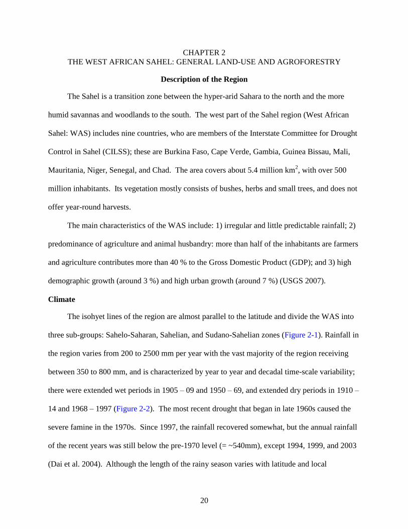
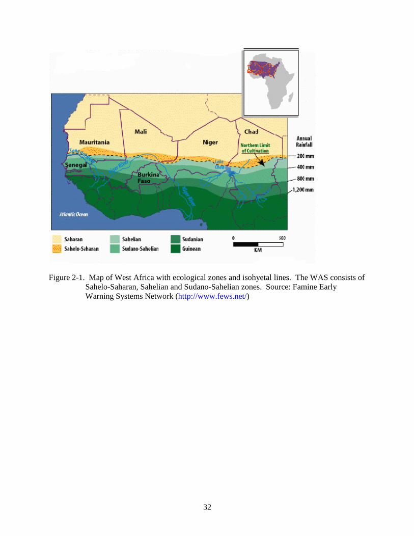
The isohyet lines of the region are almost parallel to the latitude and divide the WAS into
three sub-groups: Sahelo-Saharan, Sahelian, and Sudano-Sahelian zones (Figure 2-1). Rainfall in
the region varies from 200 to 2500 mm per year with the vast majority of the region receiving
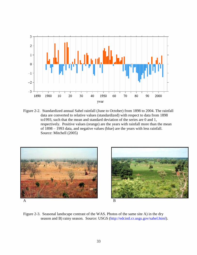
between 350 to 800 mm, and is characterized by year to year and decadal time-scale variability;
there were extended wet periods in 1905 – 09 and 1950 – 69, and extended dry periods in 1910 –
14 and 1968 – 1997 (Figure 2-2). The most recent drought that began in late 1960s caused the
severe famine in the 1970s. Since 1997, the rainfall recovered somewhat, but the annual rainfall
of the recent years was still below the pre-1970 level (= ~540mm), except 1994, 1999, and 2003
(Dai et al. 2004). Although the length of the rainy season varies with latitude and local
21
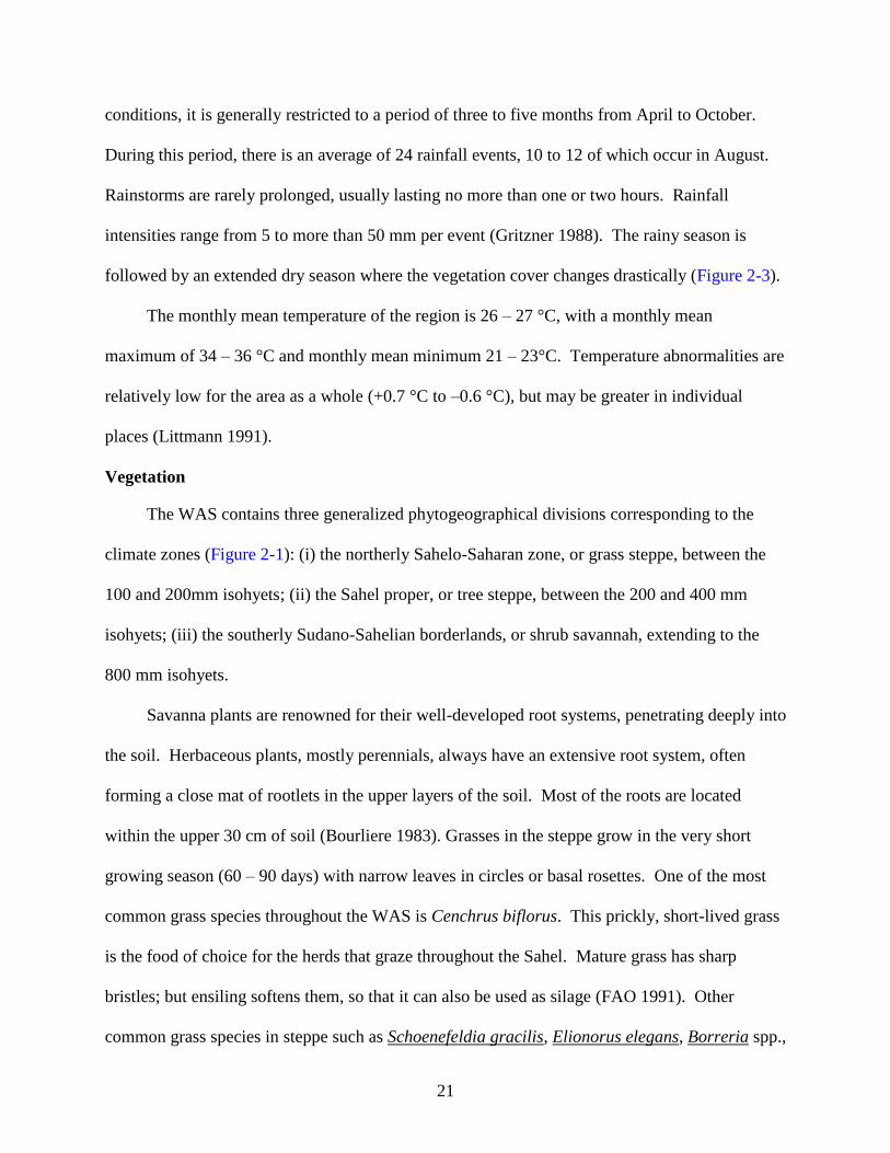
conditions, it is generally restricted to a period of three to five months from April to October.
During this period, there is an average of 24 rainfall events, 10 to 12 of which occur in August.
Rainstorms are rarely prolonged, usually lasting no more than one or two hours. Rainfall
intensities range from 5 to more than 50 mm per event (Gritzner 1988). The rainy season is
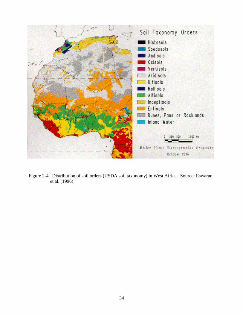
followed by an extended dry season where the vegetation cover changes drastically (Figure 2-3).
The monthly mean temperature of the region is 26 – 27 °C, with a monthly mean
maximum of 34 – 36 °C and monthly mean minimum 21 – 23°C. Temperature abnormalities are
relatively low for the area as a whole (+0.7 °C to –0.6 °C), but may be greater in individual
places (Littmann 1991).
Vegetation
The WAS contains three generalized phytogeographical divisions corresponding to the
climate zones (Figure 2-1): (i) the northerly Sahelo-Saharan zone, or grass steppe, between the
100 and 200mm isohyets; (ii) the Sahel proper, or tree steppe, between the 200 and 400 mm
isohyets; (iii) the southerly Sudano-Sahelian borderlands, or shrub savannah, extending to the
800 mm isohyets.
Savanna plants are renowned for their well-developed root systems, penetrating deeply into
the soil. Herbaceous plants, mostly perennials, always have an extensive root system, often
forming a close mat of rootlets in the upper layers of the soil. Most of the roots are located
within the upper 30 cm of soil (Bourliere 1983). Grasses in the steppe grow in the very short
growing season (60 – 90 days) with narrow leaves in circles or basal rosettes. One of the most
common grass species throughout the WAS is Cenchrus biflorus. This prickly, short-lived grass
is the food of choice for the herds that graze throughout the Sahel. Mature grass has sharp
bristles; but ensiling softens them, so that it can also be used as silage (FAO 1991). Other
common grass species in steppe such as Schoenefeldia gracilis, Elionorus elegans, Borreria spp.,
22
are also used as fodders. In the south, where the savannah replaces the steppe, the tall perennial
grasses such as Andropogon gayanus as well as annual grasses with long cycles such as
Pennisetum pedicellatum, Andropogon pseudapricus, and Diheteropogon hagerupiiare are
common. These grasses grow rapidly up to 2.5 m in height, but natural bush fires control the
reserves. Some of these species are introduced as ornamental or fodder species in the US
(Pennisetum pedicellatum, called Kyasuma grass) and Australia (Andoropogon gayanus), and
because of their rigorous spread, they are invasive species.
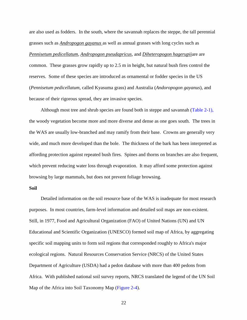
Although most tree and shrub species are found both in steppe and savannah (Table 2-1),
the woody vegetation become more and more diverse and dense as one goes south. The trees in
the WAS are usually low-branched and may ramify from their base. Crowns are generally very
wide, and much more developed than the bole. The thickness of the bark has been interpreted as
affording protection against repeated bush fires. Spines and thorns on branches are also frequent,
which prevent reducing water loss through evaporation. It may afford some protection against
browsing by large mammals, but does not prevent foliage browsing.
Soil
Detailed information on the soil resource base of the WAS is inadequate for most research
purposes. In most countries, farm-level information and detailed soil maps are non-existent.
Still, in 1977, Food and Agricultural Organization (FAO) of United Nations (UN) and UN
Educational and Scientific Organization (UNESCO) formed soil map of Africa, by aggregating
specific soil mapping units to form soil regions that corresponded roughly to Africa's major
ecological regions. Natural Resources Conservation Service (NRCS) of the United States
Department of Agriculture (USDA) had a pedon database with more than 400 pedons from
Africa. With published national soil survey reports, NRCS translated the legend of the UN Soil
Map of the Africa into Soil Taxonomy Map (Figure 2-4).
23
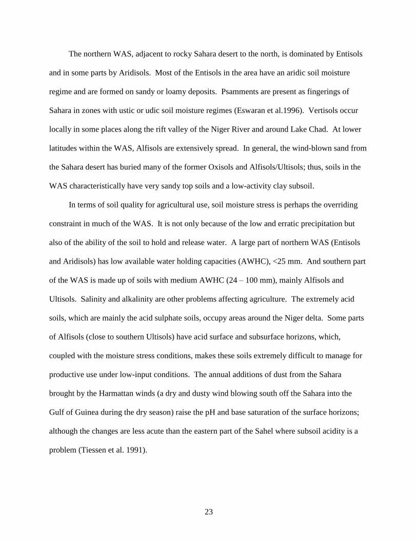
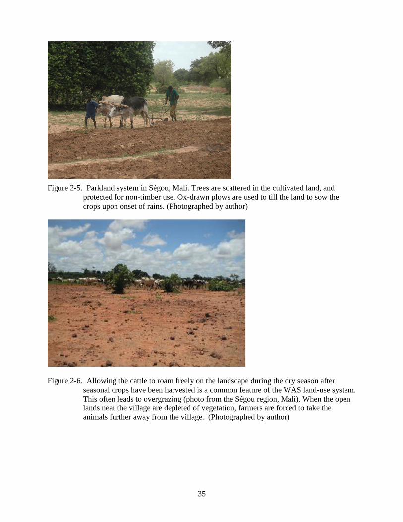
The northern WAS, adjacent to rocky Sahara desert to the north, is dominated by Entisols
and in some parts by Aridisols. Most of the Entisols in the area have an aridic soil moisture
regime and are formed on sandy or loamy deposits. Psamments are present as fingerings of
Sahara in zones with ustic or udic soil moisture regimes (Eswaran et al.1996). Vertisols occur
locally in some places along the rift valley of the Niger River and around Lake Chad. At lower
latitudes within the WAS, Alfisols are extensively spread. In general, the wind-blown sand from
the Sahara desert has buried many of the former Oxisols and Alfisols/Ultisols; thus, soils in the
WAS characteristically have very sandy top soils and a low-activity clay subsoil.
In terms of soil quality for agricultural use, soil moisture stress is perhaps the overriding
constraint in much of the WAS. It is not only because of the low and erratic precipitation but
also of the ability of the soil to hold and release water. A large part of northern WAS (Entisols
and Aridisols) has low available water holding capacities (AWHC), <25 mm. And southern part
of the WAS is made up of soils with medium AWHC (24 – 100 mm), mainly Alfisols and
Ultisols. Salinity and alkalinity are other problems affecting agriculture. The extremely acid
soils, which are mainly the acid sulphate soils, occupy areas around the Niger delta. Some parts
of Alfisols (close to southern Ultisols) have acid surface and subsurface horizons, which,
coupled with the moisture stress conditions, makes these soils extremely difficult to manage for
productive use under low-input conditions. The annual additions of dust from the Sahara
brought by the Harmattan winds (a dry and dusty wind blowing south off the Sahara into the
Gulf of Guinea during the dry season) raise the pH and base saturation of the surface horizons;
although the changes are less acute than the eastern part of the Sahel where subsoil acidity is a
problem (Tiessen et al. 1991).
24
In addition to the moisture stress and alkalinity/acidity, there are several other soil-related
constraints common in the WAS contributing to low productivity. These include: 1) inherently
low nutrient storage capacities (cation exchange capacities, CECs) due to the low-activity
kaolintic clay minerals present or the overall low clay contents, 2) low equilibrium soil organic
matter levels due to intensive cultivation without adequate biomass return and high surface soil
temperatures, 3) the presence of large amounts of free aluminum and iron oxides which reduces
the availability of phosphate to plants (Gritzner 1988; de Alwis 1996)
Traditional Farming Systems and Agroforestry in the WAS
The traditional farming systems in the WAS are rain-fed, low external input operations.
Farmers use traditional agricultural methods: use of domestic wastes, farmyard manure, crop
rotations, and the incorporation of trees on farmlands. There is a considerable variety of crops
grown in Sahelian agricultural systems, including: grains, such as millet (Pennisetum glaucum),
sorghum (Sorghum bicolor), fonio (Digitaria exilis), rice (Oryza glaberrima and Oryza sative),
sesame (Sesamum indicum), and safflower (Carthamus tinctorius); garden crops, such as
eggplant (Solanum melongena), broad beans (Vicia faba), okra (Abelmoschus esculentus), carrots
(Daucus carota), chick-peas (Cicer arietinum), pigeon peas (Cajanus cajan), cowpeas (Vigna
unguiculata), ground nut (Arachis hypogaea), yams (Dioscorea spp.), calabash (Lagenaria
siceraria), leeks (Allium ampeloprasum), melons (Cucurbitaceae Family), etc. Cultivated tree
crops including dates (Phoenix dactylifera), figs (Ficus spp.), lemons (Citrus spp.), mulberries
(Morus spp.), and various gums (Acacia spp.) are also common (Gritzner 1988; ICRISAT 2007).
25
Traditional Agroforestry Practices
Bush fallow/shifting cultivation
Shifting cultivation refers to the land-management practice where a period of cropping
(cropping phase) is alternated with a period in which the soil is rested (fallow phase). This
system has been traditionally practiced in the WAS, as well as other tropical and semi-tropical
regions of the world (Nair 1993). First, the clearing is done using axes or machetes and only
herbaceous plants, saplings and undergrowth are cut. When the cut material is dried and burned,
the cleared area is planted with crops like yams, sorghum, millet, maize (Zea mays), and cassava
(Manihot esculenta). The land is cultivated for one to four years after which it returns to fallow.
The regrowth of natural vegetation rejuvenates the soil through nutrient cycling, addition of litter
and suppression of weeds (Ferguson 1983).
In general, the fallow phase is much longer than the cropping phase. However, recent
rapid population growth in the WAS countries (from 2.5 to 3.0 %) requires additional cultivated
land, often at the expense of fallow and pastureland. Over the years, the fallows became greatly
reduced both in area and duration, putting in jeopardy the return of vegetative cover for the
build-up of soil fertility (Kaya 2000).
Parkland system
Another traditional land-use system, sometimes overlapped with tree-combined fallow
system, is known as the ‗agroforestry parklands‘ system. Parklands are generally understood as
landscapes in which mature trees occur scattered in cultivated or recently fallowed fields (Boffa
1999). Farmers grow crops around and underneath of the trees (Figure 2-5). These trees are
selectively left or regenerated by farmers because of the variety of functions (mostly non-timber
use) such as food and medicine (Table 2-2). Parkland trees can also contribute to temperature
amelioration and to prevention of soil erosion (Jonsson et al. 1999). Parklands occupy a vast
26
land area, representing a large part of the agricultural landscape under subsistence farming in the
WAS and it is the predominant agroforestry system. For example, the agroforestry parkland
system occupies about 90 % of the agricultural land area in Mali (Cissé, 1995), and in Burkina
Faso, parklands are found throughout settled zones where agriculture is practiced.
Parklands are most often characterized by the dominance of one or a few tree species.
Species composition is generally more diverse and variable, however, in areas located farther
away from villages and only occasionally cultivated. Common species in the WAS are Acacia
senegal, Adansonia digiata, Anogeissus leiocarpus, Balanites aegyptiaca, Bombax costatum,
Borassus aethiopum, Ceiba pentandra, Diospyros mespiliformis, Elaeis guineensis, Faidherbia
albida, Hyphaene thebaica, Lannea microcarpa, Parkia biglobosa, Sclerocarya birrea,
Tamarindus indica, Vitellaria paradoxa, Vitex doniana, and Ziziphus mauritiana (Table 2-2)
(Boffa 1999).
Improved Agroforestry Practices
The expansion of rain-fed agriculture results in soil erosion through the removal of
vegetative cover and physical disturbance. Wind and water erosion is extensive in many parts of
the WAS. Practically every country of Africa is prone to desertification, but the Sahelian
countries at the southern fringe of the Sahara are particularly vulnerable (Reich et al. 2001). Soil
nutrients are removed through crops, erosion, and leaching by rainfall, without replenishment by
additions or regeneration under natural fallow. Inappropriate tillage and cultural practice reduce
soil infiltration and retention of water, which further degrade the land (de Alwis 1996). Also,
deforestation accelerates the land degradation as trees and shrubs are cut to satisfy the
construction, fuel, and fodder requirements of the cultivators and their livestock. In the WAS,
farmers/pastoralists usually graze their animals in the open area without any control (Figure 2-6).
Degraded land spreads as these animals go further after eating the vegetation around the villages.
27
Consequently, forest and woodland areas are rapidly declining by an estimated 1.5 % per year on
average of West African countries (FAO 2000).
Prevention of land-degradation by controlled grazing and afforestation is often discussed
and tried sporadically throughout the WAS as projects, financed mainly by international donor
communities and agencies (Oba et al. 2000). However, local participation has often been short-
lived and management not successful because little consideration was given to why farmers keep
browsing the animals and do not protect or grow trees. Gradually, there has been a growing
awareness that trees be regarded as an integral component of an overall farming system and that
a complex decision-making environment with interdisciplinary interactions is needed (Boffa
1999).
Adoption of improved land-use systems such as agroforestry has been recommended and
tried for rehabilitation of the degraded soils in various parts of the WAS (Roose et al. 1999; Lal
2004a). No-till farming and improved fallow involving short-rotation woody and/or other
perennial species are increasingly studied. Improved fallow rests land from cultivation, as in
natural fallows, but the vegetation comprises planted and managed species of leguminous trees,
shrubs, and herbaceous cover crops. These vegetation and the roots are expected to reduce the
soil nutrient loss or even to replenish them both chemically and physically, and to sustain crop
production with shorter fallow period (Bationo et al. 2000; Kaya and Nair 2001). Farming
systems that promote organic manure inputs (including litters from woody plants) and tree-
cropping systems have also been tried (Breman and Kessler 1997). As such, agroforestry
practices involving incorporation of woody plants (both indigenous and exotic species) on
cultivated land as intercrops, fences, shelter belts, and/or fodder resources are recognized as a
28
major technique to ameliorate the spreading land degradation in the WAS. Details of the
improved agroforestry practices being introduced in the study region are described in Chapter 4.
29
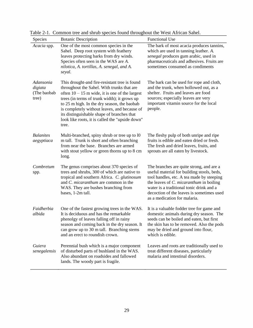
Table 2-1. Common tree and shrub species found throughout the West African Sahel.
Species Botanic Description Functional Use
Acacia spp. One of the most common species in the
Sahel. Deep root system with feathery
leaves protecting barks from dry winds.
Species often seen in the WAS are A.
nilotica, A. tortillas, A. senegal, and A.
seyal.
The bark of most acacia produces tannins,
which are used in tanning leather. A.
senegal produces gum arabic, used in
pharmaceuticals and adhesives. Fruits are
sometimes consumed as condiments
Adansonia
digiata
(The baobab
tree)
This drought-and fire-resistant tree is found
throughout the Sahel. With trunks that are
often 10 – 15 m wide, it is one of the largest
trees (in terms of trunk width); it grows up
to 25 m high. In the dry season, the baobab
is completely without leaves, and because of
its distinguishable shape of branches that
look like roots, it is called the "upside down"
tree.
The bark can be used for rope and cloth,
and the trunk, when hollowed out, as a
shelter. Fruits and leaves are food
sources; especially leaves are very
important vitamin source for the local
people.
Balanites
aegyptiaca
Multi-branched, spiny shrub or tree up to l0
m tall. Trunk is short and often branching
from near the base. Branches are armed
with stout yellow or green thorns up to 8 cm
long.
The fleshy pulp of both unripe and ripe
fruits is edible and eaten dried or fresh.
The fresh and dried leaves, fruits, and
sprouts are all eaten by livestock.
Combretum
spp.
The genus comprises about 370 species of
trees and shrubs, 300 of which are native to
tropical and southern Africa. C. glutinosum
and C. micaranthum are common in the
WAS. They are bushes branching from
bases, 1-2m tall.
The branches are quite strong, and are a
useful material for building stools, beds,
tool handles, etc. A tea made by steeping
the leaves of C. micaranthum in boiling
water is a traditional tonic drink and a
decoction of the leaves is sometimes used
as a medication for malaria.
Faidherbia
albida
One of the fastest growing trees in the WAS.
It is deciduous and has the remarkable
phenolgy of leaves falling off in rainy
season and coming back in the dry season. It
can grow up to 30 m tall. Branching stems
and an erect to roundish crown.
It is a valuable fodder tree for game and
domestic animals during dry season. The
seeds can be boiled and eaten, but first
the skin has to be removed. Also the pods
may be dried and ground into flour,
which is edible.
Guiera
senegalensis
Perennial bush which is a major component
of disturbed parts of bushland in the WAS.
Also abundant on roadsides and fallowed
lands. The woody part is fragile.
Leaves and roots are traditionally used to
treat different diseases, particularly
malaria and intestinal disorders.
30
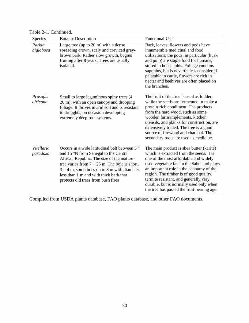
Table 2-1. Continued.
Species Botanic Description Functional Use
Parkia
biglobosa
Large tree (up to 20 m) with a dense
spreading crown, scaly and creviced grey-
brown bark. Rather slow growth, begins
fruiting after 8 years. Trees are usually
isolated.
Bark, leaves, flowers and pods have
innumerable medicinal and food
utilizations, the pods, in particular (husk
and pulp) are staple food for humans,
stored in households. Foliage contains
saponins, but is nevertheless considered
palatable to cattle, flowers are rich in
nectar and beehives are often placed on
the branches.
Prosopis
africana Small to large leguminous spiny trees (4 – 20 m), with an open canopy and drooping
foliage. It thrives in arid soil and is resistant
to droughts, on occasion developing
extremely deep root systems.
The fruit of the tree is used as fodder,
while the seeds are fermented to make a
protein-rich condiment. The products
from the hard wood, such as some
wooden farm implements, kitchen
utensils, and planks for construction, are
extensively traded. The tree is a good
source of firewood and charcoal. The
secondary roots are used as medicine.
Vitellaria
paradoxa
Occurs in a wide latitudinal belt between 5 °
and 15 °N from Senegal to the Central
African Republic. The size of the mature
tree varies from 7 – 25 m. The bole is short,
3 – 4 m, sometimes up to 8 m with diameter
less than 1 m and with thick bark that
protects old trees from bush fires
The main product is shea butter (karité)
which is extracted from the seeds. It is
one of the most affordable and widely
used vegetable fats in the Sahel and plays
an important role in the economy of the
region. The timber is of good quality,
termite resistant, and generally very
durable, but is normally used only when
the tree has passed the fruit-bearing age.
Compiled from USDA plants database, FAO plants database, and other FAO documents.
31
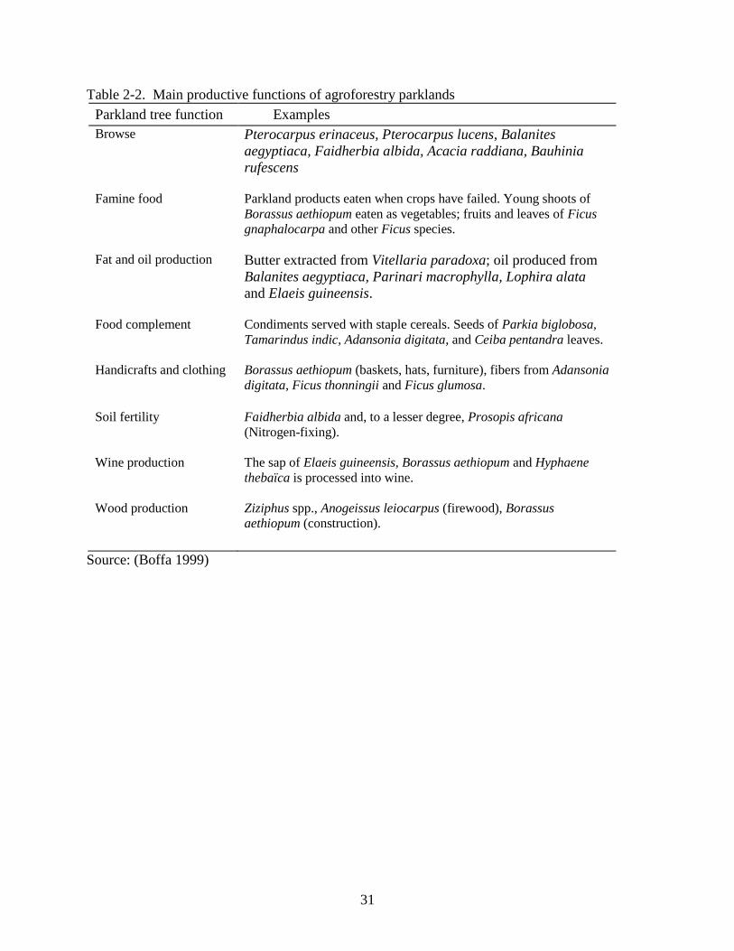
Table 2-2. Main productive functions of agroforestry parklands
Parkland tree function Examples
Browse Pterocarpus erinaceus, Pterocarpus lucens, Balanites
aegyptiaca, Faidherbia albida, Acacia raddiana, Bauhinia
rufescens
Famine food Parkland products eaten when crops have failed. Young shoots of
Borassus aethiopum eaten as vegetables; fruits and leaves of Ficus
gnaphalocarpa and other Ficus species.
Fat and oil production Butter extracted from Vitellaria paradoxa; oil produced from
Balanites aegyptiaca, Parinari macrophylla, Lophira alata
and Elaeis guineensis.
Food complement Condiments served with staple cereals. Seeds of Parkia biglobosa,
Tamarindus indic, Adansonia digitata, and Ceiba pentandra leaves.
Handicrafts and clothing Borassus aethiopum (baskets, hats, furniture), fibers from Adansonia
digitata, Ficus thonningii and Ficus glumosa.
Soil fertility Faidherbia albida and, to a lesser degree, Prosopis africana
(Nitrogen-fixing).
Wine production The sap of Elaeis guineensis, Borassus aethiopum and Hyphaene
thebaïca is processed into wine.
Wood production Ziziphus spp., Anogeissus leiocarpus (firewood), Borassus
aethiopum (construction).
Source: (Boffa 1999)
32
Figure 2-1. Map of West Africa with ecological zones and isohyetal lines. The WAS consists of
Sahelo-Saharan, Sahelian and Sudano-Sahelian zones. Source: Famine Early
Warning Systems Network (http://www.fews.net/)
33
Figure 2-2. Standardized annual Sahel rainfall (June to October) from 1898 to 2004. The rainfall
data are converted to relative values (standardized) with respect to data from 1898
to1993, such that the mean and standard deviation of the series are 0 and 1,
respectively. Positive values (orange) are the years with rainfall more than the mean
of 1898 – 1993 data, and negative values (blue) are the years with less rainfall.
Source: Mitchell (2005)
(
A B
Figure 2-3. Seasonal landscape contrast of the WAS. Photos of the same site A) in the dry
season and B) rainy season. Source: USGS (http://edcintl.cr.usgs.gov/sahel.html).
34
Figure 2-4. Distribution of soil orders (USDA soil taxonomy) in West Africa. Source: Eswaran
et al. (1996)
35
Figure 2-5. Parkland system in Ségou, Mali. Trees are scattered in the cultivated land, and
protected for non-timber use. Ox-drawn plows are used to till the land to sow the
crops upon onset of rains. (Photographed by author)
Figure 2-6. Allowing the cattle to roam freely on the landscape during the dry season after
seasonal crops have been harvested is a common feature of the WAS land-use system.
This often leads to overgrazing (photo from the Ségou region, Mali). When the open
lands near the village are depleted of vegetation, farmers are forced to take the
animals further away from the village. (Photographed by author)
36
CHAPTER 3
LITERATURE REVIEW: CARBON SEQUESTRATION POTENTIAL OF AGROFORESTRY
SYSTEMS IN THE WEST AFRICAN SAHEL (WAS)
Overview
Carbon (C) sequestration has become a hotly debated and widely researched topic during
the recent past. Consequently, voluminous literature is available on the subject. The review in
this chapter is limited to issues that are most relevant to the present study. Following a general
overview of the topic, the chapter presents brief descriptions of various methodologies that are
currently recognized and/or debated for C measurement and accounting, although not all of these
were used in this study. Then, studies estimating C storage in agroforestry systems (both
biomass C and soil C) in the WAS and other ecoregions are presented. Given that the potential
of C sequestration cannot be fully evaluated without integrating both biophysical and
socioeconomic sides of acceptability, socioeconomic issues related to C sequestration activities
through agroforestry are also discussed.
C Sequestration as a Climate-Change-Mitigation Activity
The international response to climate change started in full with the establishment of the
United Nations Framework Convention on Climate Change (UNFCCC) in 1992. Five years
later, 159 countries signed a treaty called the Kyoto Protocol, which commits the 38 signatory
developed countries to reduce their collective greenhouse gas (GHG) emissions by at least 5%
compared to the 1990 level by the period 2008 – 2012. The agreement came into force on
February 16, 2005, following its ratification by Russia on November 18, 2004. As of April
2007, a total of 169 countries and other governmental entities have ratified the agreement. A
unique characteristic of the Kyoto protocol is that it allows the amount of CO2 sequestered by
forests to be counted towards emission targets.
37
Tropical forest conversion contributes as much as 25 % of net annual CO2 emissions
globally (Palm et al. 2004). Removing this atmospheric C and storing it in the terrestrial
biosphere is, thus, one option for mitigating the emission of this GHG. A recent assessment of
Rose et al. (2007), referenced by Intergovernmental Panel on Climate Change (IPCC)‘s newest
report, suggests that land-based mitigation – agriculture, forestry, and biomass liquid and solid
energy substitutes – can be cost-effective land mitigation options. And, it can contribute over the
century 94 to 343 Pg C equivalent of greenhouse gas emission abatement, which is 15 to 40
percent of the total abatement required for stabilization.
Agroforestry for C sequestration
Under the Kyoto Protocol‘s Article 3.3, further defined by Marrakesh Accord in 2001,
agroforestry was recognized as an option of mitigating GHGs. Since then, the C sequestration
potential of agroforestry systems has attracted greater attention from both industrialized and
developing countries. It is attractive because of its applicability to a large number of people and
areas currently in agriculture, as well as its perceived potential for reducing pressure on natural
forests. Also, Clean Development Mechanism (CDM), defined in Article 12 of the Protocol adds
the attractiveness, because the CDM provides for Annex I Parties (industrialized countries which
have emission reduction goals) to implement project activities that reduce emissions in non-
Annex I Parties (developing countries), in return for certified emission reductions (CERs)
(UNFCCC 2007). Since agroforestry is traditionally and widely practiced in developing
countries, it is feasible/easy options for both developing and developed groups of countries to
start as mitigation projects under the CDM.
However, as stated by Makundi et al. (2004) and several others, estimating the amount of
C sequestered by agroforestry poses unique challenges. In addition to the complexity caused by
diverse factors such as climate, soil type, tree-planting densities, and tree management as well as
38
specific difficulties arising from requirements for monitoring, verification, leakage assessment
and the establishment of credible baselines, agroforestry estimations are beset by the problem of
estimating the area under agroforestry practices. Nevertheless, the IPCC (2000) estimated that
630 million ha of unproductive croplands and grasslands could be converted to agroforestry
worldwide, with the potential to sequester 391,000 Mg of C per year by 2010 and 586,000 Mg C
per year by 2040.
Although the credibility of conceptual models and theoretical benefits has been
demonstrated, C sequestration potential is still a little-studied characteristic of agroforestry
systems (Nair and Nair 2003). More studies examining how much C can be sequestered/stored
in various agroforestry systems around the world are needed. Several studies and reviews from
different regions of the world have discussed agroforesty‘s benefits and limitations for C
sequestration (Schroeder 1994; Dixon 1995; Albrecht and Kandji 2003), but only very few deal
with comprehensive comparisons of different practices in each ecoregion.
Due to the difficult physical environment and lack of research infrastructure, agroforestry
systems in the WAS are one of the least documented topics regarding C sequestration potential.
Lal (1999) estimated the potential for sequestering C in the region was, as in most other
drylands, fairly low, between 0.05 – 0.3 Mg C ha-1
yr-1. The estimate, however, included a
variety of uncertainties related to future shifts in global climate, land-use and land cover, and the
poor performance of trees and crops on poor soils in the region.
In the WAS, impacts of population pressure, over-grazing and continuous drought are
causing severe land degradation. Consequently, biomass C stocks steadily decline within land-
use/land cover. Opportunities for C gains in the region are, thus, often discussed in the context
of agricultural fertility and sustainability of farming systems, which involve agroforestry such as
39
tree-crop-livestock integration and fallowing practices (Manlay et al. 2002; Woomer et al.
2004a).
Methodologies for C Sequestration Measurements
Efforts to accurately measure C in forests are gaining global attention as countries seek to
comply with agreements under the UNFCCC. Many methodologies have been put forth to
quantify the amount of C in forests (Beer et al. 1990; MacDicken 1997; Brown 1999), and are
best based on permanent sample plots laid out in a statistically sound designs. This is often quite
difficult in agroforestry systems and is one of the reasons why there are few studies that actually
measure the amount of C (Montagnini and Nair 2004). Practically, there are four possible
approaches to measuring the amount of C stored as a result of particular land management
practice; 1) Direct on-site measurements of biomass, soil C, or C flux, 2) Indirect remote sensing
techniques, 3) Modeling, 4) Default values for land/activity based practices (Table 3-1).
Most of these approaches were originally developed to estimate the amount of C in forest
stands. Several pilot projects are ongoing to ensure that C that is sequestered for the long term in
economically viable agroforestry systems is reliably measured. The factors that influence which
approach is used in a specific project depends on technical availability, budget for the
measurement, and size of the land to be estimated. Since most of C mitigation projects are either
still in the pilot stage or implemented on a small scale, direct measurement approaches are most
commonly used and reported.
Direct On-site Measurement
Direct on-site measurement includes field sampling and laboratory measurements of total
C in the biomass and soil. These measurements (including inventory data used for the remote
sensing, modeling or default values) are in effect ―snapshots‖ of C stored at the time of the
40
inventory. How to calculate/determine the amount of ―sequestered‖ C over a certain period is
another issue, and discussed in the ―Accounting Methods‖ section.
Inventory
In general, C in forest or agroforestry systems can be divided into four groups; 1)
Aboveground biomass, 2) Belowground biomass, 3) Soil C, 4) Litter fall/crop residue. Methods
to collect and calculate the sample data from project sites have been standardized by many
reports and studies (MacDicken 1997; Roshetko et al. 2002).
Data for the four C categories are collected by timber cruising and sampling of herbaceous
vegetation, soil, and standing litter crop at sample plots (Shepherd and Montagnini 2001; Brown
2002; Tiepolo et al. 2002). Also, for existing forests, many tropical countries have at least one
inventory of all or part of their forest area that could be applied for agroforestry systems,
although many of the inventories are more than 10 years old and very few have repeated
inventories. Data from these inventories can be converted to biomass C depending on the level
of detail reported (Brown, 1997).
Conversion and estimation
For aboveground biomass, trees are divided by compartments: leaves, branches and trunks,
and measured in dry weight (Beer et al. 1990), because each compartment has unique C content
and decomposition rate. Although this is the most accurate method, these inventories are often
too time-consuming and costly.
Alternatively, biomass expansion factors or allometric biomass equations are often used,
because they require only stem wood information such as diameter at breast height (DBH).
These equations exist for practically all forests types of the world, especially in the temperate
zone (Sharrow and Ismail 2004). But, because of the very general nature of these equations, they
lack accuracy; they are, at best, approximations. For an agroforestry system, Shroeder (1994)
41
used a ratio of total aboveground biomass to stem wood biomass of 2.15 derived from many
previous studies. Where tree-stocking density was high (>500 trees ha-1
) and the growth cycle or
rotation length was relatively long (>10 years), i.e., for conditions more similar to those for a
forest plantation, a ratio of 1.6 was used in the study to estimate total aboveground biomass.
Total C content is usually estimated based on the assumption that 45 to 50 % of branch and stem
dry biomass is C, and that 30 % of dry foliage biomass is C (Shepherd and Montagnini 2001;
Schroth et al. 2002).
Herbaceous vegetation and standing litter are also collected from sample plots and weighed
to calculate their C content. It is often assumed in inventories that this vegetation type
contributes little to the total biomass C of a forest and it is often ignored. However, the
contribution of herbaceous vegetations is often larger in agroforestry systems than in forests,
such as green manure from trees in natural systems. The amount of litterfall, pruning residues,
and crops largely depends on the season and rotation period (Beer et al. 1990). Thus, it is
difficult to estimate using general ratios as used in the stem biomass estimation.
For belowground C, it is divided into two main categories; root biomass, and soil C
(mainly organic matter). Although methods for measuring aboveground biomass are well
established, measurement of root biomass is difficult and time-consuming in any ecosystem and
methods are generally not standardized (Ingram and Fernandes 2001). A review of the literature
shows that typical methods include spatially distributed soil cores or pits for fine and medium
roots and partial to complete excavation and/or allometry for coarse roots. The distinction
between live and dead roots is generally not made and root biomass is usually reported as total.
Moreover, sampling depths are not standardized, yet the depth selected in a given study is
assumed to capture practically all roots (Brown 2002).
42
Root biomass is often estimated from root:shoot ratios (R/S). It can be calculated by
sample plot measurements, but there are also lists of reference data. A literature review by
Cairns et al. (1997) included more than 160 studies covering tropical, temperate and boreal
forests that reported both root biomass and aboveground biomass. The mean R/S based on these
studies was 0.26, with a range of 0.18 (lower 25 % quartile) to 0.30 (upper 75 % quartile). The
R/S did not vary significantly with latitudinal zone (tropical, temperate, and boreal), soil texture
(fine, medium and coarse), or tree type (angiosperm and gymnosperm).
Soil C samples should be collected from each layer, dry-weighed and analyzed for its C
contents by recommended laboratory procedures. To calculate C stocks per unit area, the C
content in the soil is multiplied by the bulk density of the respective soil layer. By itself, C
sequestration in agricultural soils is expected to make only modest contributions globally (e.g., 3
– 6 % of total fossil C emissions) (Paustian et al. 1997). However, this amount can be
significantly varied through management such as fallow phase, erosion, tillage, or tree
incorporation.
Indirect Remote Sensing Techniques
Even where field measurement methodologies are established, agricultural/forestry
practices are inherently dispersed over a wide geographic area. Staffing costs for monitoring and
verification of land-use practices over such a wide area could prove to be cost prohibitive.
Because direct field measurements can be expensive, the use of indirect remote sensing
techniques is being considered. A range of remote data collection technologies is now available
including satellite imagery and aerial photo-imagery from low flying airplanes. Sensors that can
measure the height of the canopy or vertical structure will be needed along with the more
traditional sensors on Landsat or Spot satellites in order to improve the ability of remotely
sensing biomass (Brown 2002).
43
A promising advance in remote measurements of forest/agroforest biomass C is a scanning
lidar (a pulsed laser), a relatively new type of sensor that explicitly measures canopy height.
This sensor is able to monitor 98 % of the earth‘s closed canopy forests (Brown 2002). Another
promising advance in the remote sensing area, especially at smaller scales (thus, probably more
appropriate for agroforestry systems), couples dual-camera digital videos (wide-angle and zoom)
with a pulse laser profiler, data recorders, and differential GPS (geographical positioning system)
mounted on a single engine plane (Brown 2002). The plane flies aerial transects across the area
with several fixed altitude to take the images data, and these images are used to create 3D models
of the terrain. From these measurements, crown area, tree height, or number of stems per area of
agroforestry systems would be much more easily and accurately estimated.
Modeling
Since total direct inventory is site-specific and can be expensive, another way to lower the
cost of estimating C amount is developing a model. To date, several models have been
developed that simulate C budgets and fluxes at the level of the forest stands. These models
range from very detailed ecophysiological models used in climate impact assessment, to very
general empirical, descriptive models of C budgets within forest stands. None of these models
has been widely disseminated, and none of them accepted as a possible standard for C crediting
projects so far.
One of the most recognized and utilized models by various projects, including agroforestry
projects, is CO2FIX which was developed by researchers of Wageningen University,
Universidad Nacional Autonoma de Mexico, Centro Agronomico Tropical de Investigacion y
Ensenanza (CATIE), and European Forest Institute (EFI). This model is a user-friendly tool for
dynamically estimating the C sequestration potential of forest management, agroforestry and
44
afforestation projects. The model is a multi-cohort ecosystem-level model based on C
accounting of forest stands, including forest biomass, soils and products (Masera et al. 2003).
Another common methodological approach to estimating mitigation potential more broadly
is known as comprehensive mitigation assessment process (COMAP). The COMAP model
requires the projection of land-use scenarios for both a baseline and for a mitigation case. It
requires data on a per hectare basis on C sequestration in vegetation, detritus, and forest
products, soils and also on GHG emission avoidance activities (Makundi and Sathaye 2004).
Default Values for Land/Activity Based Practices
This approach is the broadest, nation-level approach, which uses default values for certain
land-based activities for estimating C storage. A land-use based accounting system would focus
on the changes in C stocks on managed lands during a defined time period (Dixon et al. 1994a).
Default values would be assigned to a particular tract of land based upon county or regional level
research on the average sequestration likely to result from specific agricultural or conservation
measures in that area. Various values could be assigned to such broad land management
activities as forest, cropland, or grazing management. Under this approach, field measurements
of C storage changes in individual fields would not be necessary. Land-use monitoring can be
readily measured by remote sensing techniques, eliminating the need for many field inspectors.
However, field plots may need to be set up, representing the average or a range of conditions for
the entire project area, and used as a reference to provide actual estimates to increase the
accuracy of large-scale projects.
Accounting Methods
In order to assert that agroforestry systems are an important C sequestration method, the
amounts measured in agroforestry systems must result in long-term changes in terrestrial C
storage and CO2 concentrations in the atmosphere (Masera et al. 2003). Thus, the time frame
45
and C accounting methods are very important; but they are also often controversial issues at
international negotiations of climate change.
Approaches to Assessing C Sequestration Performance
Fluxes of C and flow summation
Balancing the annual flux from a source of emissions by uptake in a forestry/agroforestry
project is conceptually the simplest way of providing offsets. In this approach, offsets are
‗delivered‘ to the C credit market on an annual basis, according to the emissions avoided,
relative to the project baseline. However, since fluxes of C associated with forestry/agroforestry
are irregular, it may be difficult to match the uptake by a particular project to an industrial source
of emissions.
Furthermore, national or international authorities must assign permanent C storage status
to project areas, such that the owners are liable for any emissions, as well as eligible for credits.
Without such status C might be accumulated in the growing phase of the forestry cycle, only to
be lost at the end of rotation (Tipper and De Jong 1998).
Average changes in the stocks of C
The pilot phase of most sequestration projects is assessed on the basis of the long-term
average increase in the stocks of terrestrial C relative to the baseline (Kursten and Burschel
1993; van Noordwijk et al. 2002), expressed as tC according to the equation: Average net C
storage (tC) = ∑(C stored in project – C stored in baseline) in tC / n (years)
The stock change method calculates the difference in C stocks between a project and its
baseline at a given point in time. A key advantage of both methods is that it focuses on the
sustainability of changing the stock of C stored in vegetation and soils. However, long-term C
storage is not easily defined, and there may be considerable argument over the assumptions
about risks and possible future changes in management. The timing of the emission reduction
46
relative to the emissions that are supposed to be offset may be problematic, since there may be a
time lag of years to decades between the establishment of the offset project and actual uptake of
the C.
Cumulative C storage
The cumulative storage approach is based on an understanding of C cycle dynamics and
radiative forcing of the atmosphere. The total warming effect of a given emission is determined
by the cumulative presence of GHG in the atmosphere; in other words the product of
concentration and time. In the case of CO2, terrestrial and oceanic sinks take up C previously
emitted, over time. Assuming the dynamics of the C cycle remain stable, most CO2 emitted at
the present will be absorbed within 100 years, and the cumulative radiative forcing produced by
this emission will be proportional to the area under the depletion curve, expressed in tC.years.
Calculation of this area provides an estimate of the cumulative C storage that would be required
to offset an emission of 1 tC at the present time. This method avoids both the necessity of
making questionable assumptions about the long-term balance of C in forests/agroforests, and
the practical difficulties of implementing flux-based incentive systems. However, international
agreements on the conversion factor for tC.years per tC emission and the time limit for crediting
the effect of a given project are required (Tipper and De Jong 1998).
Other accounting methods
In addition to these relatively simple conventional methods, alternative approaches have
been proposed to better address the temporal dimension of C storage, such as equivalence-
adjusted average storage, stock change crediting with ton-year liability adjustment, equivalence-
factor yearly crediting, equivalence-delayed full crediting, and ex-ante ton-year crediting (De
Jong 2001). Most of these are based on adopting a two-dimensional measurement unit that
reflects storage and time, i.e., ton-C year. The general concept of the ton-year approach is in the
47
application of a factor to convert the climatic effect of temporal C storage an equivalent
(equivalent factor) amount of avoided emissions.
Technical Problems and Uncertainties
There are a number of shortcomings of conventional methods for estimating/accounting
the C in a system that need to be considered. These include the uncertainties related to future
shifts in global climate, land-use and land cover, the poor performance of trees and crops, varied
environments, pests and diseases such as nematodes. For example, the amount of C remaining
belowground at the end of the tree rotation, and the amount of C sequestered in products created
from the harvested wood, including their final disposition are often not included in the
accounting methods discussed above (Johnsen et al. 2001). Oren et al. (2001) reported that after
an initial growth spurt, trees grew more slowly and did not absorb as much C from the
atmosphere as expected. They concluded that assessment of future C sequestration should
consider the limitations imposed by soil fertility as well as interactions with nitrogen deposition.
In addition to these uncertainties, there are some concerns about the impacts of
agroforestry in other GHGs. The wide-scale use of woody legumes, which is common in
agroforestry systems, might result in release of nitrous oxide (N2O)(Choudhary et al. 2002),
although it does not seem to be as strong an impact as N- fertilization (Mosier et al. 2004). N2O
is known to have a global warming potential 200 – 300 times higher than that of CO2. Similarly,
pasture and rice paddy cultivation in agroforestry systems can produce significant quantities of
methane (CH4), another strong GHG (20 – 60 times higher impact than CO2), on a global scale
(Dixon, 1995).
48
Biomass C Sequestration
Studies in Various Ecoregions
The amount of C sequestered in an agroforestry system depends largely on the nature of
the system put in place, the structure and function of which are determined by environmental and
socioeconomic factors (Albrecht and Kandji. 2003). Other factors influencing C storage include
tree species and system management (Delaney and Roshetko1998; Roshetko et al. 2002). Palm
et al. (2004) compared the amount of C stored (above-ground) in different ecological systems
(Table 3-2). To compare the rotation of the different land-use systems, time-averaged C of each
system was used.
C stocks in the vegetation of the primary forests averaged 300 Mg C ha-1
, and that of
logged or managed forests ranged from a high of 228 Mg C ha-1
in Cameroon to a low of 93 Mg
C ha-1
in Indonesia. Time-averaged aboveground C for the different land-uses ranged from 50 –
90 Mg C ha-1
in long-fallow shifting cultivation and complex agroforestry systems, to 30 – 60
Mg C ha-1 in simple agroforestry systems and most tree plantations and medium-fallow
rotations. These are considerably larger than those for annual crops or pastures.
Studies in West Africa
In a review of C sequestration in tropical agroforestry systems, Albrecht and Kandji (2003)
estimated that agrosilvicultural system could sequester 29 – 53 Mg C ha-1
in humid tropical
Africa. A case study in Cameroon (humid west and central Africa) showed that the cacao
(Theobroma cacao) agroforest is superior to the alternative food crop production system (slash-
and-burn), both in C sequestration and below- and above-ground bio-diversity. Total biomass in
cacao agroforest was 304 Mg ha-1
, compared to crop fields (84 Mg ha-1
) (Duguma et al. 2001).
Compared to C gains in the humid tropics, the benefits of agroforestry in the WAS, such as
parklands or improved fallow seem to be less. A simulation study in Senegal compared the C
49
gains after 25 years from protecting parkland systems (2.48 Mg C ha-1
) with that of rotating
crops with Luecaena spp. fallow planting (6.35 Mg C ha-1
) (Tschakert 2004). Although drylands
as whole are believed to provide a substantial opportunity for C offsets especially in soil C,
because of their large area (47.2 % of land in the world) and low human populations (Lal 2004b),
most studies in the Sahel region have concluded that the potential for C gains per unit area
through agroforestry is relatively low (Walker and Desankar 2004;Woomer et al. 2004b)
compared with other ecoregions.
In general, introducing trees into agricultural systems is expected to increase water and
nutrient availability, because trees can fix nitrogen, retrieve water and nutrients from below the
rooting zone of crops, and reduce water and nutrient losses from leaching and erosion (Buresh
and Tian 1997). This tree effect has been demonstrated in various agroforestry systems in the
semiarid region. However, this added value was lowest where it is most needed, in resource-
poor environments: the competition between woody plants and crops is strong (Kater et al. 1992;
Breman and Kessler 1997). Water constraints are the strongest limitations for C sequestration in
the WAS. Several local tree species such as Acacia tortilis, Guiera senegalensis, Pterocarpus
lucens have been planted in grasslands of the region for sequestering C, but their capacity to
grow has been shown to be constrained by moisture availability (Woomer et al. 2004a). The
capacity of exotic dryland tree species to afforest the WAS is also uncertain.
Since the moisture and nutrient levels of the study field are expected to be low, the tree
growth and the consequent C storing will not be extremely high, either, compared with more
moist parts of West Africa. However, the amounts of C sequestered as a result of specific land-
uses are mostly unknown in the WAS, thus, it is worthwhile to conduct the research to have a
reference data for future C sequestration projects.
50
Soil C Sequestration
Recently, research focused on C sequestration potential in terrestrial ecosystems has been
shifting from biomass C to soil C, because soil is recognized as an important storage (sink) for C
and studies estimating biomass have accumulated for various ecosystem (including
agroecosystem and plantation forests), while the dynamics of soil C is much less known.
Studies of Soil C Stock and Dynamics
The comparison study of C sequestration potential by Palm et al. (2004) (Table 3-2) also
measured soil C storages. On average, 45 Mg C ha-1
were found in the forest systems studied (0
– 20 cm depth), and 80 – 100 % of that C storage in agroforestry systems; 80 % in pastures; 90 –
100 % in long-fallow cycles; 65 % in short-term fallows, and 50 % or less in annual crops and
degraded grasslands. Rosalina et al. (1997) reported a mean of 104 Mg C ha-1
for home gardens
in North Lampung, Indonesia, and that 58 % of the stock is soil C. The soil C sampling depth of
these studies is usually on surface, up to 20cm. Although the surface soil is the major part of
which soil organic carbon (SOC) is found, it may not be deep enough to capture all the tree roots
influence on soil C (Jobbagy and Jackson 2000). But because of the labor intensity and the
relatively low soil C density, deeper soil C tends to be ignored.
Storage of soil C is rather easy to quantify and/or estimate, but detecting soil C flux
including its turn-over time is much more difficult and has not been studied much. Most current
models of soil organic matter (SOM) dynamics assume that equilibrium C stocks are linearly
proportional to C inputs, i.e. there are no assumptions of soil C saturation. Six et al. (2002a)
questioned the validity of this assumption for projecting longer term SOM dynamics, and
developed the proposition that physiochemical characteristics inherent to soils define the
maximum protective capacity of SOM pools. Methodologies such as fractionation and C isotope
measurements are being developed for quantifying and identifying the characteristics of soil C
51
dynamics, and are actively discussed in the soil science arena (Balesdent et al. 1998; Del Galdo
et al. 2003; Powers and Veldkamp 2005).
Soil fractionation: There are various ways to separate SOM into labile and recalcitrant
pools, and these methods rely on chemical, physical, or biological separation, and many of them
are used sequentially in analyses (McLauchlan and Hobbie 2004). Chemical fractionation
separates soil C into different resistance class to decomposition by using acid,
permanganate(KMnO4), or hot water, (Moody et al. 1997; Ghani et al. 2003). Physical
fractionation separates labile and recalcitrant fractions by either size or density. Sieving is used
to size differentiation and flotation with a dense liquid is usually used to measure light fraction
which is considered to be labile (Six et al. 1998). Biological separation uses microbes to
separate labile SOC from recalcitrant SOC under
controlled temperature and moisture conditions,
assuming that microbes will mineralize the most labile C first, with recalcitrant C being
mineralized later (Alvarez and Alvarez 2000). With applying these methods, many examine the
impact of land-use change on soil C storage and dynamics. For example, it is possible to assess
how land-use rotation (including fallow) or change of management such as reduction of tillage
can effectively protect recalcitrant soil C, so that enhance soil C sequestration (Pikul. et al. 2007;
Zibilske and Bradford 2007).
13C isotope measurement: During photosynthesis, CO2 fixation of C3 plants discriminates
against the heavier isotope 13
C more than do C4 plants, which result in different stable carbon
isotope composition (13
C), 13
C/12
C ratio relative to that found in the PDB (Pee Dee belemnite),
for their plant material. This composition value of C3 plants is between –23 and –34 , whereas
C4 plants ranges from –9 to –17 (Eleki et al. 2005). Negative values of
13C indicate that the
plant material is depleted in 13
C compared with the PDB standard.
Using this theoretical
52
expected difference between the measured 13
C values, it is possible to calculate the proportion
of C4 derived material and C3 derived material in biomass or soil C (Balesdent et al. 1998). This
method has been used for soil C research to assess vegetation composition change (Dzurec et al.
1985) or to follow the dynamics (Harris et al. 2001). Mcdonagh et al. (2001) measured how
SOM from original vegetation (forest: C3 plants) were diminished after continuous cultivation of
maize (Zea mays: C4 plants). In agroforestry system, Jonsson et al. (1999) used this method to
prove the positive influence of trees (C3 plants) on SOM increase at millet (Pennisetum
glaucum: C4 plants) cropland.
Soil C in the WAS
In the WAS, most of the soils have low activity clay, with low water retention and are
susceptible to soil erosion and compaction, as described in Chapter 2. Organic matter content of
these soils has been depleted due to overgrazing, agricultural mismanagement, deforestation and
overexploitation of the natural resources. As a result, soil organic C stock density in West Africa
is very low (4.2 – 4.5 kg C m-2
), compared with the world average (10.9 – 11.6 kg C m-2
), and
relatively lower even when compared to the average for Africa (6.4 – 6.7 kg C m-2
) (Batjes
2001).
Soil degradation is a major obstacle for agricultural productivity and thus sustainable
development of the WAS. The possibility of enhancing C sequestration through improved soil
management has been discussed academically and at international workshops, as part of the
search for agroecosystem sustainability in the region. Among soil-nutrients studies in Africa, tree
integration into croplands is often recommended for soil amelioration (Onim et al. 1990; Tiessen
et al. 1991; Manlay et al. 2002). Kang et al. (1999) reported Grilicidia sepium and Leucaena
leucocephala increased surface soil organic C by 15 % compared to sole crops in a 12-year
hedgerow intercropping trial on a Nigerian Alfisol. Parkland system studies affirm that the soil
53
under the trees is richer in organic matter content and several cations compared to adjacent tree-
less sites (Kater et al. 1992; Jonsson et al. 1999).
Soil amelioration by land management in the WAS is, however, often met with limited
success when it comes to maintaining or increasing soil nutrient and C stocks. The potential for
C sequestration in a given soil and agroecological zone is proportional to the original reserves
present under undisturbed conditions. Breman and Kessler (1997) compared the added values of
woody plants in croplands or pastures between Sahel zone and wetter Sudan zone. They
concluded possibilities to improve the soil organic matter status are more limited in Sahel, due to
resource-poor environments and competition for water between woody plants and crops or
pasture. Because of the slow establishment of a woody plant community and the rapid turnover
of organic matter, a long ―transition period‖ is necessary under the conditions in Sahel.
Improved fallow studies also suggest that a long period would be needed to amend soil physical
conditions of the highly degraded soil in the WAS (Buresh and Tian 1998; Ringius 2002; Kaya
and Nair 2004).
Soil C sequestration is not recognized as a mitigation means during the first commitment
period of the Kyoto Protocol (2008 – 2012), although political pressure to reverse this situation
has been growing. In his review of soil C sequestration in Africa, Ringius (2002) stated that sub-
Saharan Africa would not profit significantly from soil C sequestration under the Clean
Development Mechanism (CDM) as long as the land-use pressures due to a rapidly growing
population and poverty remain unsolved. Profitability of the soil C sequestration project is
uncertain, since cost benefit studies of the sequestration activities have not been conducted.
There is a need to launch long-term (>10 yr) field experiments and pilot projects for soil C
54
sequestration as well as to develop a land resources information system in the WAS, geared
towards CDM and/or C sale.
Socioeconomic Implications
To analyze the socioeconomic feasibility of the agroforestry practices for mitigation
projects, analysis tools, i.e. models, are needed. Economic models of different scales used for
the studies in various ecoregions are summarized here. Although the number of studies is small,
the case studies and possibility of using these economic models in the WAS are also examined.
Economic Models
In most studies of C sequestration, agroforestry is regarded as one of the forest
management options for potential C sequestration. There are few studies specifically discussing
economic models of C sequestration in agroforestry systems; instead, models designed for
managed forests are usually applied (Masera et al. 2003). These economic models for
accounting C sequestration projects can be categorized into two different spatial scales.
National/global scale
Apart from the C sequestration potential per se of agroforestry systems, the potential for
realizing this assumed benefit depends largely on the availability of land which can be changed
to agroforestry from land with less C storage, such as agricultural fields. Attempts to estimate
the global potential for increasing C sinks through land-use change had been conducted at the
global, national, and regional levels for more than a decade (Dixon et al. 1994b; Sathaye et al.
2001; Godal et al. 2003). These studies use simple integrated model structure, based on
biophysical and economic information. In this kind of large spatial scale, empirical model
schemes such as the Holdridge life zone system (LZS) can be used as a guideline for organizing
vegetation data (Pfaff et al. 2000). For economic factors such as the price of land, cost of land-
use change, and timber price, national census information are generally available. Information
55
on land-use and trends of change, collected from national surveys or satellite/remote sensing
data, are integrated and the overall economic impacts are examined.
Results are presented in several different ways. Dixon (1995) presented the potential C
storage (over 50 year rotation) and initial project financial costs for agroforestry systems for
ecoregions of selected nations in terms of $/Mg C. Some studies estimate total investment cost
in actual dollar amounts for developed countries to achieve their reduction goals (Baron and
Lanza 2000, Godal et al. 2003), and others estimate each country‘s investment in $ ha-1
, or
internal rate of return (IRR) (%) (Dixon 1995; Sathaye et al. 2001).
Micro/site-specific scale
At this level, more detailed economic estimation is conducted based on data from the
specific target (project) field. Various factors of benefits and costs are individually counted.
There are three different time frames for counting these costs and benefits of C sequestration
projects: point estimates, partial equilibrium estimates, and general equilibrium approaches.
Many of the point-estimate studies provide undiscounted private costs and benefits of the
project‘s implementation in $ ha-1
. These studies usually count only direct inputs and outputs,
including land cost. Estimating opportunity costs to compare with other land-use options is often
done (Tomich et al. 2002). Most of these studies reveal little about how costs might change
throughout the project with time, or if the project were to expand or be repeated. Thus, the
estimates tend to be biased towards the low end.
The Scolel Té project, conducted in Mexico, is one of the few long-term and
comprehensive economic impact studies on this subject. It serves as an example agroforestry
project for calculating the costs related to implementing a C sequestration project in rural
environments dominated by resource-poor small-scale farmers, who are expected to be major
players in agroforestry worldwide. The study accounts for costs of project design, the time
56
required to explain to farmers the project objectives, C related inventories, and the cost of
baseline setting, which are often ignored in similar estimate analysis (De Jong et al. 2004).
These equilibrium studies usually present the results as discounted costs in $/Mg C with long-
term average sequestered C as Mg C ha-1
.
For estimating much longer scales than one cycle of agroforestry rotation, computer-based
modeling methods are usually used. There are several models such as CO2FIX and
WaNULCAS for estimating the dynamics of C sequestration over decades to centuries and some
are applicable to agroforestry (Van Noordwijk et al. 2002; Masera et al. 2003). Wise and Cacho
(2005) used the WaNULCAS model for ecological estimates combined with their economic
model, including variables such as local discount rate, firewood price, and labor cost, and
simulated the long-term economic value of switching land-use from agricultural system to
agroforestry system in Indonesia. They include expected C prices into its economic analysis, and
presented net present values (NPV) in $ ha-1
of several different setting (management options).
Agroforestry systems in temperate areas are usually analyzed in a very different way.
Compared with developing countries in the tropics, the C credit sale through forestation is not
likely to be economically feasible soon in the temperate area. Thus, C sequestration tends to be
considered as an environmental benefit (non-market value, or subject to receive the subsidies).
Studies to estimate the benefits of C sequestration using models that are generally used for these
environmental commodities seem to be the current research trends (Stainback and Alavalapati
2000; Alavalapati et al. 2004).
Feasibility in West Africa
West African countries‘ GHG emissions are currently negligible in global terms, due to the
low level of development and industrialization. As a result, emission reduction opportunities
57
remain few, and are mainly in lessening the negative impact on the climate resulting from land-
use change and deforestation.
For C offset projects, however, the risk of shifting from cropping to more C-beneficial
practices seems to be high, especially for subsistence farmers who have little lands. A study of C
sequestration through agroforestry in Senegal found that the costs for resource-poor farmers are
considerably higher than those of intermediate and richer farmers, because the former often lack
the necessary assets (land, labor, and animals) to switch from current to alternative practices
(Tschakert 2007).
Many African policy makers and financial institutions express little interest in controlling
GHG emissions or adapting to changes in climate. This attitude is based on their experience that,
in general, other, more local, environmental problems have more direct influence on their
populations than climate change. Senior government officials and most members of civil society
do not understand the climate issue very well (Denton et al. 2001). Many development
practitioners remain skeptical, arguing that C brokers, national ministries and local leaders rather
than needy rural populations will benefit from C projects.
An important challenge for the WAS countries lies in that they need to be more
―attractive‖ than the other African and developing countries in order to draw and hold
investments for C sequestration projects under CDM. As discussed above, the potential C gains
in the WAS through agroforestry has been considered to be unattractive. Synergies between
development and climate change response, however, can be an answer. Agroforestry projects,
which protect soils and result in C sequestration, also provide employment opportunities for local
farmers (Hardner et al. 2000). Soil C sequestration project through agroforestry could provide a
crucial link between three international conventions: the UN Framework Convention on Climate

58
Change (UNFCCC), the UN Convention to Combat Desertification (UNCCD), and the UN
Convention on Biodiversity (UNCBD). As such, incentives can come from a much broader area
such as development assistance, other multilateral agreements and sectoral policies on energy
and agriculture.
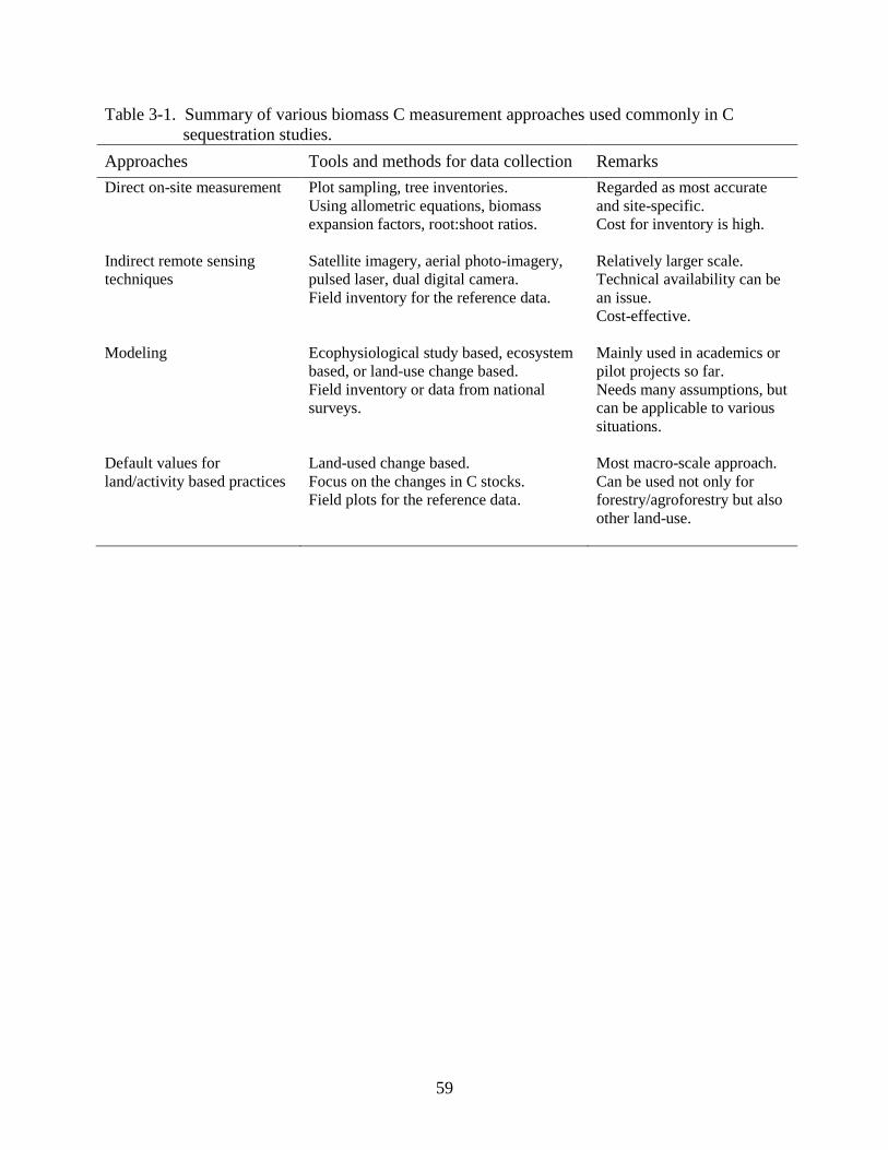
59
Table 3-1. Summary of various biomass C measurement approaches used commonly in C
sequestration studies.
Approaches Tools and methods for data collection Remarks
Direct on-site measurement Plot sampling, tree inventories.
Using allometric equations, biomass
expansion factors, root:shoot ratios.
Regarded as most accurate
and site-specific.
Cost for inventory is high.
Indirect remote sensing
techniques
Satellite imagery, aerial photo-imagery,
pulsed laser, dual digital camera.
Field inventory for the reference data.
Relatively larger scale.
Technical availability can be
an issue.
Cost-effective.
Modeling Ecophysiological study based, ecosystem
based, or land-use change based.
Field inventory or data from national
surveys.
Mainly used in academics or
pilot projects so far.
Needs many assumptions, but
can be applicable to various
situations.
Default values for
land/activity based practices
Land-used change based.
Focus on the changes in C stocks.
Field plots for the reference data.
Most macro-scale approach.
Can be used not only for
forestry/agroforestry but also
other land-use.
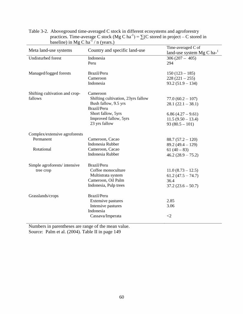
60
Table 3-2. Aboveground time-averaged C stock in different ecosystems and agroforestry
practices. Time-average C stock (Mg C ha-1
) = ∑(C stored in project – C stored in
baseline) in Mg C ha-1
/ n (years.)
Meta land-use systems Country and specific land-use Time-averaged C of
land-use system Mg C ha-1
Undisturbed forest Indonesia
Peru 306 (207 – 405)
294
Managed/logged forests Brazil/Peru
Cameroon
Indonesia
150 (123 – 185)
228 (221 – 255)
93.2 (51.9 – 134)
Shifting cultivation and crop-
fallows
Cameroon
Shifting cultivation, 23yrs fallow
Bush fallow, 9.5 yrs
Brazil/Peru
Short fallow, 5yrs
Improved fallow, 5yrs
23 yrs fallow
77.0 (60.2 – 107)
28.1 (22.1 – 38.1)
6.86 (4.27 – 9.61)
11.5 (9.50 – 13.4)
93 (80.5 – 101)
Complex/extensive agroforests
Permanent
Rotational
Cameroon, Cacao
Indonesia Rubber
Cameroon, Cacao
Indonesia Rubber
88.7 (57.2 – 120)
89.2 (49.4 – 129)
61 (40 – 83)
46.2 (28.9 – 75.2)
Simple agroforests/ intensive
tree crop
Brazil/Peru
Coffee monoculture
Multistrata system
Cameroon, Oil Palm
Indonesia, Pulp trees
11.0 (8.73 – 12.5)
61.2 (47.5 – 74.7)
36.4
37.2 (23.6 – 50.7)
Grasslands/crops Brazil/Peru
Extensive pastures
Intensive pastures
Indonesia
Cassava/Imperata
2.85
3.06
<2
Numbers in parentheses are range of the mean value.
Source: Palm et al. (2004). Table II in page 149
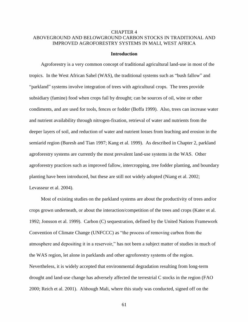
61
CHAPTER 4
ABOVEGROUND AND BELOWGROUND CARBON STOCKS IN TRADITIONAL AND
IMPROVED AGROFORESTRY SYSTEMS IN MALI, WEST AFRICA
Introduction
Agroforestry is a very common concept of traditional agricultural land-use in most of the
tropics. In the West African Sahel (WAS), the traditional systems such as ―bush fallow‖ and
―parkland‖ systems involve integration of trees with agricultural crops. The trees provide
subsidiary (famine) food when crops fail by drought; can be sources of oil, wine or other
condiments, and are used for tools, fences or fodder (Boffa 1999). Also, trees can increase water
and nutrient availability through nitrogen-fixation, retrieval of water and nutrients from the
deeper layers of soil, and reduction of water and nutrient losses from leaching and erosion in the
semiarid region (Buresh and Tian 1997; Kang et al. 1999). As described in Chapter 2, parkland
agroforestry systems are currently the most prevalent land-use systems in the WAS. Other
agroforestry practices such as improved fallow, intercropping, tree fodder planting, and boundary
planting have been introduced, but these are still not widely adopted (Niang et al. 2002;
Levasseur et al. 2004).
Most of existing studies on the parkland systems are about the productivity of trees and/or
crops grown underneath, or about the interaction/competition of the trees and crops (Kater et al.
1992; Jonsson et al. 1999). Carbon (C) sequestration, defined by the United Nations Framework
Convention of Climate Change (UNFCCC) as ―the process of removing carbon from the
atmosphere and depositing it in a reservoir,‖ has not been a subject matter of studies in much of
the WAS region, let alone in parklands and other agroforestry systems of the region.
Nevertheless, it is widely accepted that environmental degradation resulting from long-term
drought and land-use change has adversely affected the terrestrial C stocks in the region (FAO
2000; Reich et al. 2001). Although Mali, where this study was conducted, signed off on the
62
Kyoto Protocol, there has been no pilot project to document C sequestration and C credit sale in
the country.
Woomer et al (2004b) conducted a national scale C stock assessment in Senegal
(neighboring country of Mali), and found that there were opportunities for biological C
mitigation, but they were constrained by available knowledge and access to resources.
Compared with large-scale tree plantation, agroforestry is expected to be the most feasible
afforestation/reforestation project that can be conducted by the majority of resource-limited land
users (farmers) in the WAS. Because of the scarcity of on-site information, it is important to
directly measure or estimate both biomass C and soil C stocks of various agroforestry systems.
Therefore the study reported in this chapter was undertaken with two research questions:
1. How do different agroforestry systems differ in their potential for C sequestration? How
much C is stored in the traditional and improved agroforestry systems, especially comparing
above-ground and below-ground?
2. What is the overall relative attractiveness of each of the selected agroforestry systems
considering them as biological C sequestration projects?
Materials and Methods
C sequestration potential of a specified project is calculated by ―C sequestered by the
project‖ minus ―C sequestered by the baseline (without the project)‖. Since this study is not a
long-term project, it was impossible to monitor both C accumulations by the project
(agroforestry) and by non-project land-use over the time. Instead, the differences of C stock
among selected land-use systems are assumed to represent the potential of C sequestration by the
land-use change.
Study Area
This research was done in Ségou, Mali, in cooperation with the ICRAF (World
Agroforestry Centre) Field Station of Sahel Regional Programme.
63
Republic of Mali
Mali is a landlocked country with an area of 1.24-million km2; the Sahara desert occupies
60 % of it (Figure 4-1). Mali shares borders with seven countries: Mauritania, Algeria, Burkina
Faso, Ivory Coast, Guinea, Niger, and Senegal. It is a vast land of plains fed by two major
rivers, the Senegal River on its western edge and the Niger River flowing in a wide arc from
southwest to east. The population is 12.3 million with a growth rate 2.63 %, one of the highest
in the world (World Bank 2007). While most people live in rural areas, 1.2 million people live
in the capital city, Bamako; 90 % of people are Muslims. The major language is Bambara
(original language of a major ethnic group), although the official language is French.
Agriculture is the main source of livelihood for the people, with 80 % of people engaged in
agriculture or fishing (CIA 2007). Cotton is the main export product; gold and phosphate from
mines in the northern area are also traded. The per capita national income was US$ 380 in 2005.
Despite higher economic growth since 1994, Mali remains one of the world's poorest countries
— rated 174/177 in 2005, using the UNDP Human Development Index (World Bank 2007).
With the impact of current climate change and environmental degradation, the country is
vulnerable to drought and risks further desertification.
Ségou region
The City of Ségou is Mali‘s second largest urban center, located on the Niger River about
300 km northeast of Bamako. It is the capital of Ségou region, one of the eight administrative
regions of Mali (Figure 4-1). The region is located in the buffer zone of the Sahara, with 60 – 90
rainy days and 300 – 700 mm of rainfall annually (the rainfall intensity increasing from the north
to the south).
The Ségou region has seven cercles (administrative sections) and 2,218 villages. The
population of the region is about 2 million with 0.3 million living in Ségou city. Cotton
64
(Gossypium spp.) is the main crop (and product) of the region and the region is well known for it.
A large cotton mill, invested in by Chinese companies, is operating at the edge of the city. Rice
(Oryza glaberrima and Oryza sativa) is grown extensively in the irrigated area around the Niger
River (République du Mali 2005). Farmers commonly grow rain-fed pearl millet (Pennisetum
glaucum) and sorghum (Sorghum bicolor) as staple food crops.
Selected Land-use Systems for Field Data Collection
A preliminary survey was first conducted in July 2005 to identify the targeted land-use
systems and possible villages to locate on-farm plots. Five systems were selected: two parkland
agroforestry systems, two improved agroforestry systems, and an ―abandoned‖ land (degraded
land) for comparison.
Parkland systems
The major land-use in the Ségou region, as in most of other parts of the WAS, is parkland
agroforestry. Two parklands types are common: with Faidherbia albida or Vitellaria paradoxa
as the dominant tree species. These two types occupy more than 60 % of cultivated land in
Ségou region (personal communication, August 2005, with Director of Forestry Department,
Ségou). Tree density is in the range of 20 to 30 trees/ha in both systems. Crops cultivated
underneath the trees include pearl millet and sorghum, sometimes intercropped with cowpea
(Vigna unguiculata) and/or banbarra groundnut (Vigna subterranea syn. Voandzeia
subterranea).
F. albida has a unique characteristic of ―reverse‖ phenology or foliation (i.e. bearing leaves
during the hot dry season and dropping them before the rainy season), which is quite
advantageous for agroforestry: it reduces shading of crops grown underneath the tree and
possibly reduces competition for water between trees and crops, and enables farmers to grow
crops under the trees with practically very little reduction of cropped area in the intercropping
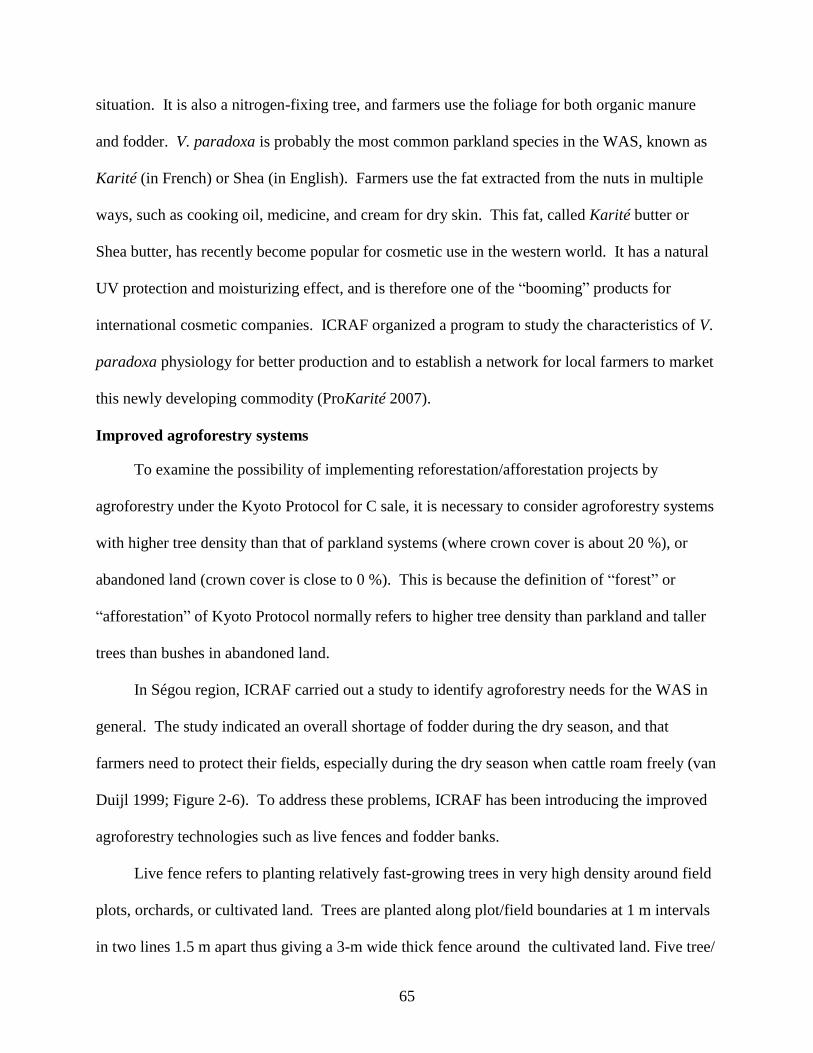
65
situation. It is also a nitrogen-fixing tree, and farmers use the foliage for both organic manure
and fodder. V. paradoxa is probably the most common parkland species in the WAS, known as
Karité (in French) or Shea (in English). Farmers use the fat extracted from the nuts in multiple
ways, such as cooking oil, medicine, and cream for dry skin. This fat, called Karité butter or
Shea butter, has recently become popular for cosmetic use in the western world. It has a natural
UV protection and moisturizing effect, and is therefore one of the ―booming‖ products for
international cosmetic companies. ICRAF organized a program to study the characteristics of V.
paradoxa physiology for better production and to establish a network for local farmers to market
this newly developing commodity (ProKarité 2007).
Improved agroforestry systems
To examine the possibility of implementing reforestation/afforestation projects by
agroforestry under the Kyoto Protocol for C sale, it is necessary to consider agroforestry systems
with higher tree density than that of parkland systems (where crown cover is about 20 %), or
abandoned land (crown cover is close to 0 %). This is because the definition of ―forest‖ or
―afforestation‖ of Kyoto Protocol normally refers to higher tree density than parkland and taller
trees than bushes in abandoned land.
In Ségou region, ICRAF carried out a study to identify agroforestry needs for the WAS in
general. The study indicated an overall shortage of fodder during the dry season, and that
farmers need to protect their fields, especially during the dry season when cattle roam freely (van
Duijl 1999; Figure 2-6). To address these problems, ICRAF has been introducing the improved
agroforestry technologies such as live fences and fodder banks.
Live fence refers to planting relatively fast-growing trees in very high density around field
plots, orchards, or cultivated land. Trees are planted along plot/field boundaries at 1 m intervals
in two lines 1.5 m apart thus giving a 3-m wide thick fence around the cultivated land. Five tree/
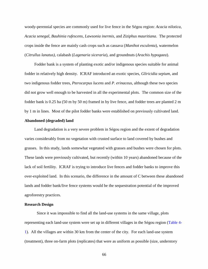
66
woody-perennial species are commonly used for live fence in the Ségou region: Acacia nilotica,
Acacia senegal, Bauhinia rufescens, Lawsonia inermis, and Ziziphus mauritiana. The protected
crops inside the fence are mainly cash crops such as cassava (Manihot esculenta), watermelon
(Citrullus lanatus), calabash (Lagenaria siceraria), and groundnuts (Arachis hypogaea).
Fodder bank is a system of planting exotic and/or indigenous species suitable for animal
fodder in relatively high density. ICRAF introduced an exotic species, Gliricidia sepium, and
two indigenous fodder trees, Pterocarpus lucens and P. erinaceus, although these two species
did not grow well enough to be harvested in all the experimental plots. The common size of the
fodder bank is 0.25 ha (50 m by 50 m) framed in by live fence, and fodder trees are planted 2 m
by 1 m in lines. Most of the pilot fodder banks were established on previously cultivated land.
Abandoned (degraded) land
Land degradation is a very severe problem in Ségou region and the extent of degradation
varies considerably from no vegetation with crusted surface to land covered by bushes and
grasses. In this study, lands somewhat vegetated with grasses and bushes were chosen for plots.
These lands were previously cultivated, but recently (within 10 years) abandoned because of the
lack of soil fertility. ICRAF is trying to introduce live fences and fodder banks to improve this
over-exploited land. In this scenario, the difference in the amount of C between these abandoned
lands and fodder bank/live fence systems would be the sequestration potential of the improved
agroforestry practices.
Research Design
Since it was impossible to find all the land-use systems in the same village, plots
representing each land-use system were set up in different villages in the Ségou region (Table 4-
1). All the villages are within 30 km from the center of the city. For each land-use system
(treatment), three on-farm plots (replicates) that were as uniform as possible (size, understory
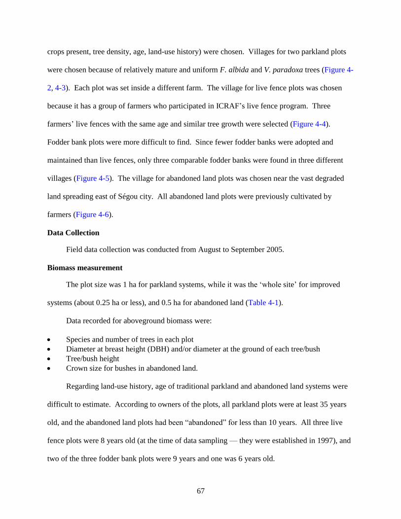
67
crops present, tree density, age, land-use history) were chosen. Villages for two parkland plots
were chosen because of relatively mature and uniform F. albida and V. paradoxa trees (Figure 4-
2, 4-3). Each plot was set inside a different farm. The village for live fence plots was chosen
because it has a group of farmers who participated in ICRAF‘s live fence program. Three
farmers‘ live fences with the same age and similar tree growth were selected (Figure 4-4).
Fodder bank plots were more difficult to find. Since fewer fodder banks were adopted and
maintained than live fences, only three comparable fodder banks were found in three different
villages (Figure 4-5). The village for abandoned land plots was chosen near the vast degraded
land spreading east of Ségou city. All abandoned land plots were previously cultivated by
farmers (Figure 4-6).
Data Collection
Field data collection was conducted from August to September 2005.
Biomass measurement
The plot size was 1 ha for parkland systems, while it was the ‗whole site‘ for improved
systems (about 0.25 ha or less), and 0.5 ha for abandoned land (Table 4-1).
Data recorded for aboveground biomass were:
Species and number of trees in each plot
Diameter at breast height (DBH) and/or diameter at the ground of each tree/bush
Tree/bush height
Crown size for bushes in abandoned land.
Regarding land-use history, age of traditional parkland and abandoned land systems were
difficult to estimate. According to owners of the plots, all parkland plots were at least 35 years
old, and the abandoned land plots had been ―abandoned‖ for less than 10 years. All three live
fence plots were 8 years old (at the time of data sampling — they were established in 1997), and
two of the three fodder bank plots were 9 years and one was 6 years old.
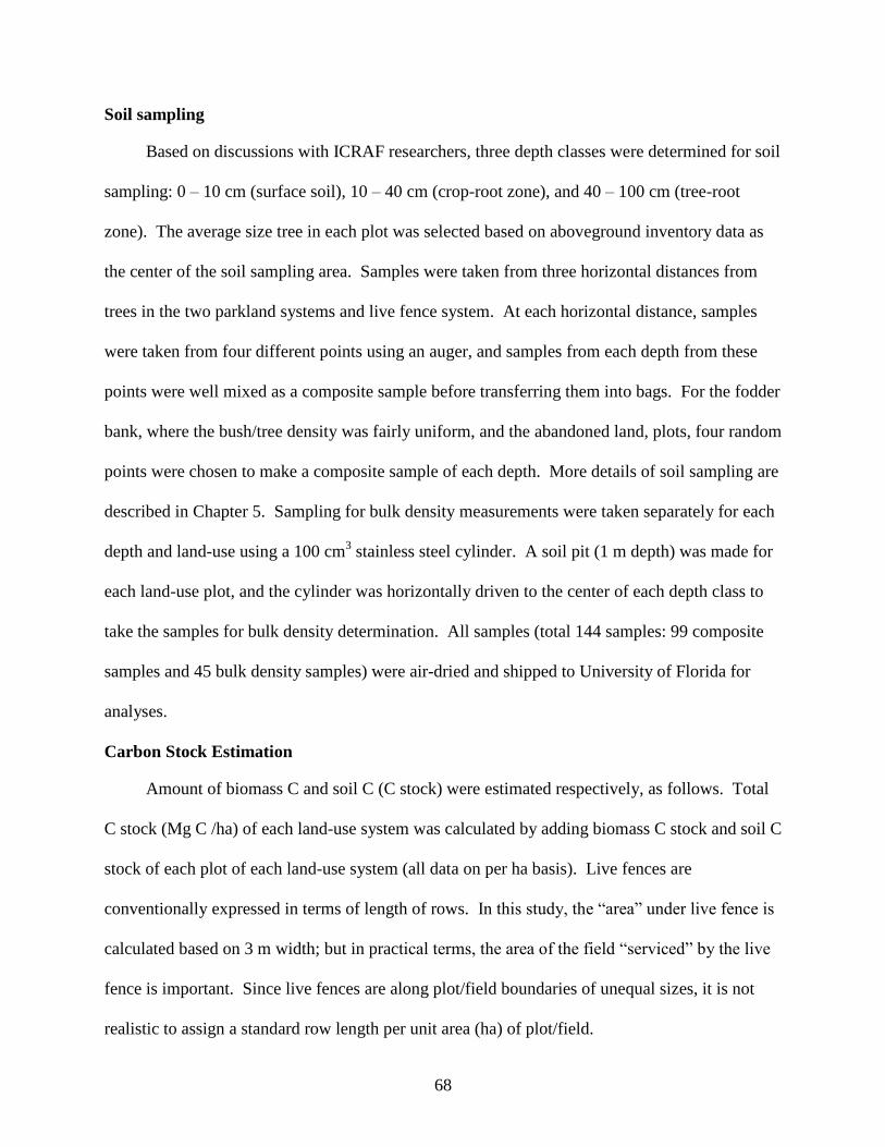
68
Soil sampling
Based on discussions with ICRAF researchers, three depth classes were determined for soil
sampling: 0 – 10 cm (surface soil), 10 – 40 cm (crop-root zone), and 40 – 100 cm (tree-root
zone). The average size tree in each plot was selected based on aboveground inventory data as
the center of the soil sampling area. Samples were taken from three horizontal distances from
trees in the two parkland systems and live fence system. At each horizontal distance, samples
were taken from four different points using an auger, and samples from each depth from these
points were well mixed as a composite sample before transferring them into bags. For the fodder
bank, where the bush/tree density was fairly uniform, and the abandoned land, plots, four random
points were chosen to make a composite sample of each depth. More details of soil sampling are
described in Chapter 5. Sampling for bulk density measurements were taken separately for each
depth and land-use using a 100 cm3 stainless steel cylinder. A soil pit (1 m depth) was made for
each land-use plot, and the cylinder was horizontally driven to the center of each depth class to
take the samples for bulk density determination. All samples (total 144 samples: 99 composite
samples and 45 bulk density samples) were air-dried and shipped to University of Florida for
analyses.
Carbon Stock Estimation
Amount of biomass C and soil C (C stock) were estimated respectively, as follows. Total
C stock (Mg C /ha) of each land-use system was calculated by adding biomass C stock and soil C
stock of each plot of each land-use system (all data on per ha basis). Live fences are
conventionally expressed in terms of length of rows. In this study, the ―area‖ under live fence is
calculated based on 3 m width; but in practical terms, the area of the field ―serviced‖ by the live
fence is important. Since live fences are along plot/field boundaries of unequal sizes, it is not
realistic to assign a standard row length per unit area (ha) of plot/field.
69
Biomass C stock
Since this study examines the potential of C sales under the Kyoto Protocol‘s Clean
Development Mechanism (CDM), methodologies used here for estimating biomass C stock are
based on the guideline published by UNFCCC (2006). Although species-specific allometric
equations are ideal, none was available for parkland trees from the study region. As an
alternative, the UNFCCC guideline recommends using the following general equations from
FAO (1997).
Tree biomass (kg) = exp (-2.134 + (2.530 lnDBH(cm))) (n = 191, R2 = 0.97) (Eq. 4-1)
In the FAO (1997) paper, there are general equations suggested for drylands. However,
those equations were developed from much smaller sets of trees in India and Mexico, and their
DBH ranges are 3 to 30 cm. F. albida and V. paradoxa trees in parkland plots of this study
greatly exceed the diameter range of these general equations. The average DBH of trees in the
plots were about 59 cm for F. albida and 42 cm for V. paradoxa. Using the dryland general
equations may cause significant over estimation of the biomass. Thus, this study follows a
method proposed by Woomer et al. (2004a) in Senegal, using Equation 4-1. This equation is
also from FAO (1997) for higher rainfall area (1500 – 4000 mm), but covers the diameter ranges
of F. albida and V. paradoxa trees in this study.
There are two options for estimating the biomass of the five live fence and one fodder bank
species. One is following UNFCCC‘s guideline, using a general equation for areas with <900
mm annual rainfall. The tree sizes are within this equation‘s DBH limits (3 – 30 cm). The
equation is:
Tree biomass (kg) = 10 ^(-0.535 + log10(π×DBH(cm)2/4)) (R
2 = 0.94) (Eq. 4-2)
70
The UNFCCC guidelines suggest using these equations when no local species allometric
equations are available.
A second option is to use the equations developed from Acacia tortillas and Acacia
ruficiens in Northwest Kenya (Coughenour et al. 1990). These are:
Log10 (g mass) = -2.26+3.98 log10 (mm stem diameter) (Eq. 4-3)
R2
=0.98 (stem diameter<15.7 mm)
Log 10 (g mass) = -0.68 +2.66 log10 (mm stem diameter) (Eq. 4-4)
R2
=0.98 (stem diameter>15.7 mm)
Although Northwest Kenya is not in the WAS, its climatic condition is much more similar
to that of the study area than to the area where the UNFCCC guideline‘s equation was developed.
Gonzalez (2001) used these Acacia spp. equations in his research at various parts of Senegal.
These two options were both tried in this study, and the results of estimated biomass C are
compared later.
For abandoned land plots, equations for Guiera senegalensis used by Seghieri et al (2005)
in Niger were adopted. G. senegalensis is the most dominant shrub species in the abandoned
land plots, and the equation was originally developed in fallows of Mali (Cissé 1980, Franklin
and Hiernaux 1991).
Foliage mass of each stem of each shrub: Blstem (g),
Basal circumference of the stem: Cstem (cm):
Blstem =1.09×Cstem (all stems of n=20 shrubs, R2 =0.82, P<0.001) (Eq. 4-5)
Stem wood dry mass: Bwstem (kg):
Bwstem =0.0037×Cstem (36 stems among n=15 shrubs, R2 =0.90, P<0.001) (Eq. 4-6)
Leaf and wood masses (Blstem and Bwstem) were then aggregated for each multi-stemmed shrub.
To calculate the amount of C in the biomass, C fraction rate of 0.5 is suggested in the
UNFCCC guideline. Belowground biomass is also estimated by using the suggested root/shoot
71
ratios, which are 0.25 for trees and 0.5 for abandoned land bushes. Biomass C stock was
calculated by adding aboveground biomass C and belowground biomass C.
Soil C stock
Soil C stock was estimated from the samples taken at each land-use‘s plots. Sub-samples
were taken from the 99 air-dried composite samples and ground. Soil C percentages of the sub-
samples (% of C weight in whole soil weight) were measured by the dry combustion method on
an automated Flash EA 1112 NC elemental analyzer (Thermo Fisher Scientific, Inc.). Then, the
soil C percentage data of each land-use of each depth class was converted to the amount of C per
ha basis with using bulk density data.
Statistical Analysis
Analysis of variance (ANOVA) by SAS PROC MIXED procedure and Turkey-Kramer
multiple comparison test were conducted to compare the C stocks of different land-use systems
and soil depth. The linear model shown below was used.
yi = μ + Li + ei
yi is the C concentration in land-use i,
μ is the population mean,
Li is the land-use (treatments), i = FA, VP, LF, FB, and AL.
FA: F.albida parkland, VP: V.paradoxa parkland, LF: live fence, FB: fodder bank, and
AL: abandoned land.
ei is the random variable error within the experiment.
Linear correlation was also tested to examine the relationship of biomass C and soil C
stock.
72
Results
C Stock in Biomass and Soil
The two parklands selected for the study were similar in tree density and the dominance of
major tree species (Table 4-2). F. albida trees were generally larger and taller than the V.
paradoxa trees in all parkland plots. Although live fence and fodder bank plots had large
numbers of trees per ha, these were proportionally calculated numbers based on small plots. The
real size of live fence plots was 0.088 ha on average (293 m length × 3 m width) with 327 trees,
and that of fodder bank plots was 0.24 ha on average with 145 G. sepium trees.
The soil C specific comparisons will be presented in detail in Chapter 5; but estimates of
soil C stock of each depth are presented, along with biomass C stock per ha basis of each system
(Figure 4-7). Statistical comparison by ANOVA showed that abandoned land had larger soil C
stock than the other four systems in every depth, although the significance varied with depth.
Estimated biomass C values of live fence and fodder bank plots from UNFCCC guideline
equations and those from Acacia spp. equations developed in Kenya were significantly different
(t-test, p<0.01) (Table 4-3). However, when each set of estimation was compared with other
three systems by ANOVA, the results were the same. The ranking of systems in order of
biomass C stock was: F. albida parkland > V. paradoxa parkland > Live fence > Fodder bank
>Abandoned land. However, the last three systems were not significantly different (Tukey-
Kramer test) even when analyzed separately.
Total C Stock
Total C (aboveground biomass C + soil C) stock of each system was calculated and
compared at three different soil depth ranges. The order among the systems and the significance
of difference varied with the depth of soil (Table 4-4). Overall, F. albida parkland had the
largest total C stock, and was significantly different from the other four systems. V. paradoxa
73
parkland had the second largest total C stock, while the difference between other systems
became less significant as deeper soil C stock was included. Also as deeper soil was taken into
account, abandoned land had more C stock relative to the other systems.
Relationship between Biomass C and Soil C
All the possible combinations of biomass C stock data and soil C stock data across the five
land-use systems were tested for their relationship:
Biomass C stock data and soil C stock data (0-10cm),
Biomass C stock data and soil C stock data (0-40cm),
Biomass C stock data and soil C stock data (0-100cm),
Biomass C stock data and soil C stock data (10-40cm), and
Biomass C stock data and soil C stock data (40-100cm).
None of the regression was significant.
Discussion
In terms of total C stock per ha, traditional agroforestry systems (parklands) are a larger
storage than improved agroforestry systems (live fence and fodder bank) or abandoned land.
Although the improved agroforestry systems are relatively young, they are not likely to store as
much as the parklands at the end of their 25 year rotation. Because branches of fodder bank trees
are annually pruned to control their height (<4 m), and live fence trees are planted in such a high
density that woody biomass accumulation per tree will be comparatively less. However, having
a large C stock does not necessarily mean having a large C sequestration potential. Traditional
parklands are very stable (long-standing), and so is the C stored. Farmers in the area are unlikely
to increase the tree density of parklands to match the UNFCCC‘s ―forest plantation‖ criteria for
sequestering more C for sale, because it will produce a negative impact on crop growth. Also it
is very difficult to convert nutrient-poor abandoned land to parklands, since silvicultural methods
are not established for these species (parkland trees are mostly natural regeneration), and
abandoned land is not fertile enough to grow crops underneath.
74
On the other hand, introducing live fences and/or fodder banks into cultivated land or
abandoned land can sequester C by increasing the tree biomass, but the extent would vary largely
by the baseline and accounting method used. Biomass C sequestered by live fence planting is a
straightforward ―addition‖ in the C equation for the site, since they are normally established on
the tree-less cultivated land (the baseline is nearly 0). The potential of fodder banks, however,
depends on initial plot condition. As in the situation for live fence, when the cultivated land is
converted to fodder bank, most of C sequestered by the fodder trees can be counted. However,
establishing fodder banks on abandoned land, as ICRAF or local government is trying to
promote, may actually result in net loss of C stock during the initial stage, because the biomass
from bushes and grasses in the abandoned land has to be removed at the time of establishment,
and it may take years for fodder trees to accumulate an amount equal to the original biomass.
Further investigations are needed on temporal C dynamics of these systems.
Soil C is not considered in the calculations of the Kyoto Protocol for its first commitment
period (2008-2012). When, rather than if, soil C is taken into account, determining baseline soil
C will be another challenge to determine and compare the C sequestration potentials of land-use
systems. Results suggest that soil-sampling depth makes a large difference in estimating the
amount of C stored per area basis, as well as the potential for C sequestration (Table 4-4). To
compare and discuss the C sequestration potential of different land-use or different ecoregions, it
will be very important to standardize sampling depth. Several studies in Africa reported that
planting trees for C sequestration will not immediately retain soil C equal to the baseline level
nor increase it in the short term (Kaya and Nair 2001; Walker and Desanker 2004). Introducing
live fences or fodder banks may increase the biomass C in the system, but may not increase soil
C. Soil C sequestration potential will be discussed in more detail in the next chapter.
75
Regarding the biomass estimation methodology, two sets of allometric equations were
used for live fence and fodder bank. The values calculated from the two methods are
significantly different from each other (UNFCCC‘s general equation is much more conservative
than Acacia species equations from Kenya). However, comparing each method‘s values with
other three land-use systems showed similar results: both live fence and fodder bank have not
(perhaps not yet) stored significant amounts of C compared with bushes of abandoned land. This
is partly because of the young age of the two systems (6 to 9 years old). The UNFCCC guideline
suggests applying the general equation only if it is impossible to find/establish local allometric
equations. The Acacia species equations are not exactly ―local‖; but they are from environments
more similar to the studied area than were the general equations. Considering the difference
between these two methods, developing the local allometric equations is likely to increase the
profits from C credit sale when the C market is introduced in the area. Obviously, substantial
research efforts are warranted in this area.

76
Table 4-1. Characteristics of the villages where the experimental plots were set up in Ségou
region, Mali.
Land-use Name of the village Position Elevation
(m) Size of the plot
Faidherbia albida
parkland
Togo
N.13.35, W. 6.31
300
1 ha
Vitellaria .paradoxa
parkland
Dakala
N.13.32, W. 6.23
297
1 ha
Live fence
Dougoucouna
N. 13.37, W.6.37
298
294m (average)
Fodder bank1
Dakala
N.13.32, W. 6.23
297
0.25 ha
Siguila N.13.28, W. 6.21 305 0.25 ha
Banankoroni N.13.35, W. 6.38 293 0.22 ha
Abandoned land
Diamaribougou
N. 13.36, W. 6.19
298
0.5 ha 1One fodder bank plot from each village
Table 4-2. Characteristics of the experimental plots (three plots average) for five-selected land-
use systems in Ségou region, Mali.
DBH (cm) Height (m) Number of
trees (ha-1
) Species composition
Faidherbia albida
parkland
59.4 (1.8)
13.0 (0.9)
21 (5.3)
Average 88.6% Faidherbia.
albida dominance
Vitellaria paradoxa
parkland
41.7 (5.9)
9.9 (0.9)
20 (0.6)
Average 80.6% Vitellaria
paradoxa dominance
Live fence
2.5 (0.5)
2.5 (0.4)
3720 (882)
Average 67.6% Acacia.
nilotica
Fodder bank
2.2 (0.5)
2.0 (1.1)
588 (277)
Gliricidia sepium average
only
Abandoned land
2.8 (0.6)
diameter at ground
1.3 (0.4)
46 (30)
Average 47.5% Guiera
senegalensis and 39.5%
Combretum micranthum
Note: Numbers in parentheses are standard deviations. Tree dominance means the percentage among the
standing trees in the plot.
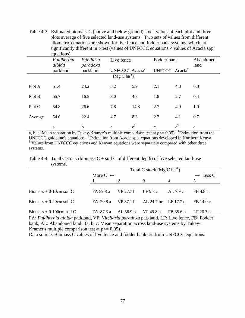
77
Table 4-3. Estimated biomass C (above and below ground) stock values of each plot and three
plots average of five selected land-use systems. Two sets of values from different
allometric equations are shown for live fence and fodder bank systems, which are
significantly different in t-test (values of UNFCCC equations < values of Acacia spp.
equations).
Faidherbia
albida
parkland
Vitellaria
paradoxa
parkland
Live fence
UNFCCC1 Acacia
2
Fodder bank
UNFCCC
1 Acacia
2
Abandoned
land
(Mg C ha
-1)
Plot A
51.4
24.2
3.2
5.9
2.1
4.8
0.8
Plot B
55.7
16.5
3.0
4.3
1.8
2.7
0.4
Plot C
54.8
26.6
7.8
14.8
2.7
4.9
1.0
Average
54.0
22.4
4.7
8.3
2.2
4.1
0.7
a
b
c
c3
c
c3
c
a, b, c: Mean separation by Tukey-Kramer‘s multiple comparison test at p<= 0.05). 1Estimation from the
UNFCCC guideline's equations. 2Estimation from Acacia spp. equations developed in Northern Kenya.
3 Values from UNFCCC equations and Kenyan equations were separately compared with other three
systems.
Table 4-4. Total C stock (biomass C + soil C of different depth) of five selected land-use
systems.
Total C stock (Mg C ha-1
)
More C ← → Less C
1 2 3 4 5
Biomass + 0-10cm soil C
FA 59.8 a
VP 27.7 b
LF 9.8 c
AL 7.9 c
FB 4.8 c
Biomass + 0-40cm soil C
FA 70.8 a
VP 37.1 b
AL 24.7 bc
LF 17.7 c
FB 14.0 c
Biomass + 0-100cm soil C
FA 87.3 a
AL 56.9 b
VP 49.8 b
FB 35.6 b
LF 28.7 c
FA: Faidherbia albida parkland, VP: Vitellaria paradoxa parkland, LF: Live fence, FB: Fodder
bank, AL: Abandoned land. (a, b, c: Mean separation across land-use systems by Tukey-
Kramer's multiple comparison test at p<= 0.05).
Data source: Biomass C values of live fence and fodder bank are from UNFCCC equations.
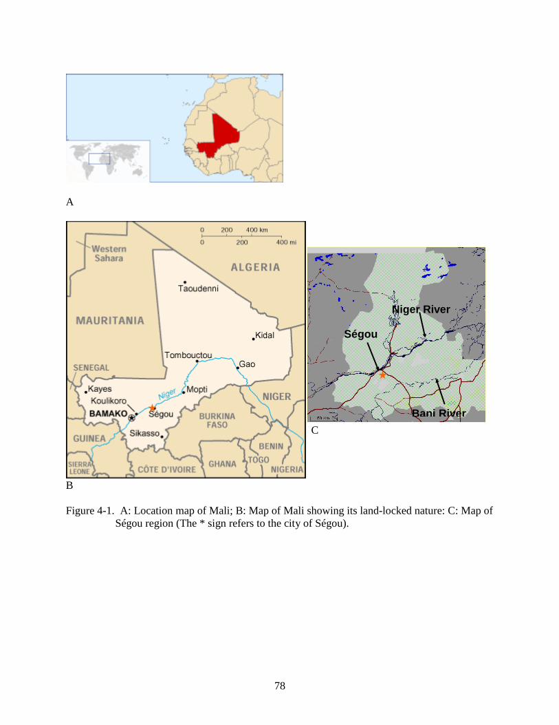
78
A
B
Figure 4-1. A: Location map of Mali; B: Map of Mali showing its land-locked nature: C: Map of
Ségou region (The * sign refers to the city of Ségou).
Ségou
Niger River
Bani River C
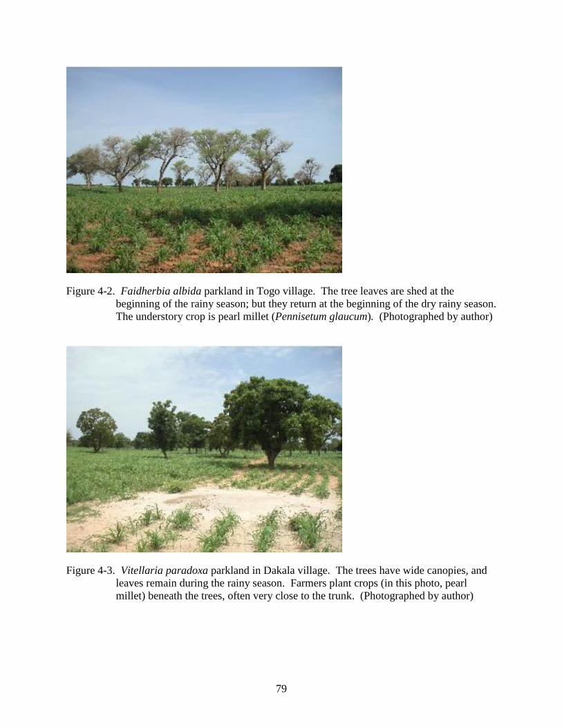
79
Figure 4-2. Faidherbia albida parkland in Togo village. The tree leaves are shed at the
beginning of the rainy season; but they return at the beginning of the dry rainy season.
The understory crop is pearl millet (Pennisetum glaucum). (Photographed by author)
Figure 4-3. Vitellaria paradoxa parkland in Dakala village. The trees have wide canopies, and
leaves remain during the rainy season. Farmers plant crops (in this photo, pearl
millet) beneath the trees, often very close to the trunk. (Photographed by author)
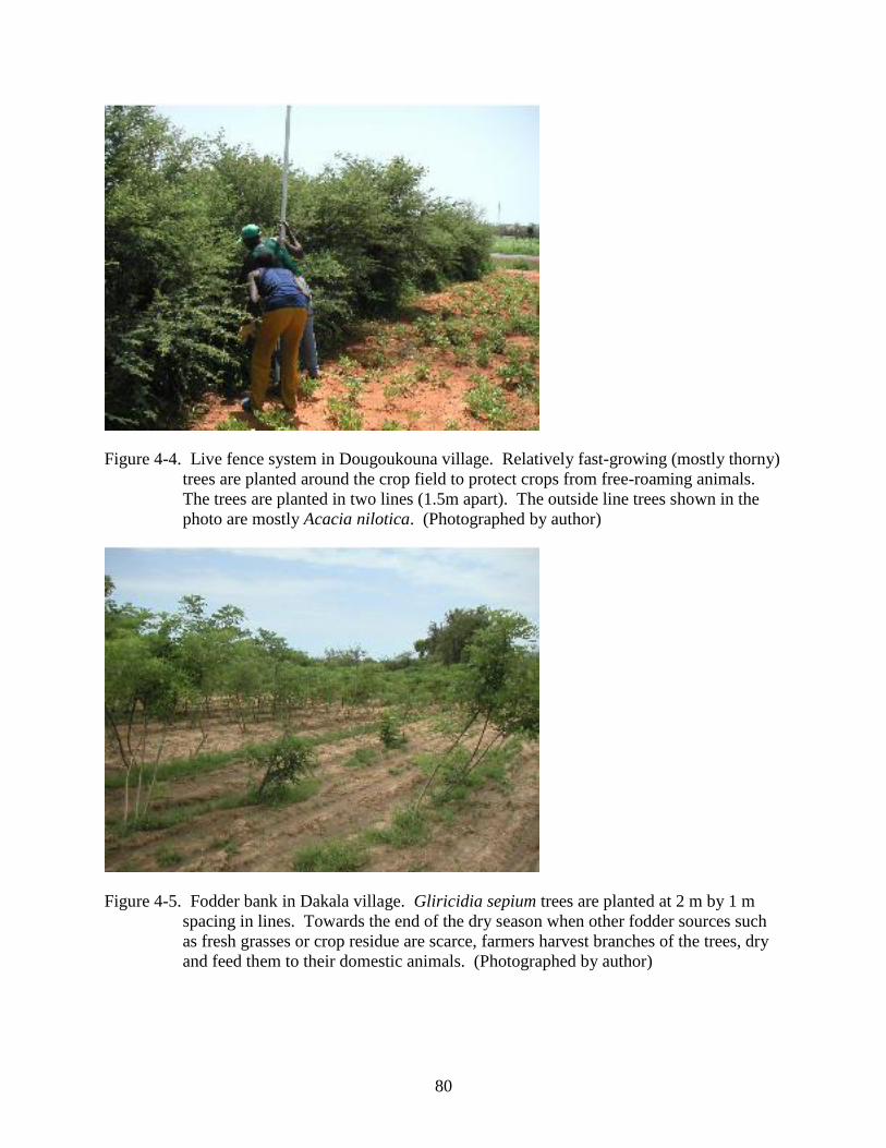
80
Figure 4-4. Live fence system in Dougoukouna village. Relatively fast-growing (mostly thorny)
trees are planted around the crop field to protect crops from free-roaming animals.
The trees are planted in two lines (1.5m apart). The outside line trees shown in the
photo are mostly Acacia nilotica. (Photographed by author)
Figure 4-5. Fodder bank in Dakala village. Gliricidia sepium trees are planted at 2 m by 1 m
spacing in lines. Towards the end of the dry season when other fodder sources such
as fresh grasses or crop residue are scarce, farmers harvest branches of the trees, dry
and feed them to their domestic animals. (Photographed by author)
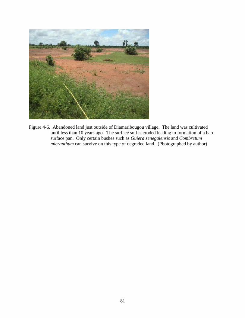
81
Figure 4-6. Abandoned land just outside of Diamaribougou village. The land was cultivated
until less than 10 years ago. The surface soil is eroded leading to formation of a hard
surface pan. Only certain bushes such as Guiera senegalensis and Combretum
micranthum can survive on this type of degraded land. (Photographed by author)
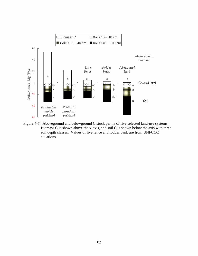
82
Figure 4-7. Aboveground and belowground C stock per ha of five selected land-use systems.
Biomass C is shown above the x-axis, and soil C is shown below the axis with three
soil depth classes. Values of live fence and fodder bank are from UNFCCC
equations.
83
CHAPTER 5
SOIL CARBON SEQUESTRATION IN DIFFERENT PARTICLE-SIZE FRACTIONS AT
VARYING DEPTHS UNDER AGROFORESTRY SYSTEMS IN MALI
Introduction
The measurement of carbon (C) content is part of the basic soil analysis procedure.
Inventory data on soil C content is available in most of the WAS countries. However, to discuss
soil C sequestration as one of the options for mitigation of atmospheric CO2, the stability of soil
C (how well C is ―captured‖ inside the soil) has to be considered. In other words, the soil C that
goes back to the atmosphere after decomposition within a month of its deposition, and that stays
in the soil for decades should not be counted as similar in terms of C credits. Characteristics
such as the stability of soil C are very controversial issues in estimating and accounting
methodologies (Ingram and Fernandes 2001; Garcia-Oliva and Masera 2004). Also, soil-
sampling depth for these accounting procedures needs to be deeper than for normal soil analysis.
The conventional soil C studies of agricultural systems mostly focus on soil organic matter in the
surface layer of 20 cm for the interests of soil fertility. But sampling of deeper soil horizon is
necessary in efforts to understand the extent of soil C protection and characteristics of various
soil C forms, especially the systems involving deep rooting plants such as trees (Jobbagy and
Jackson 2000).
In general, soil C dynamics regarding C sequestration have not yet been well studied,
although recent technological development and interests towards climate mitigation activities are
contributing to an increased number of this type of studies (Post et al. 2000; Sun et al. 2004).
Still, these studies are limited even in developed countries, and not easily available in the
research- resource limited area such as the studied region or Africa in general. The studies of
this nature that have been conducted so far have been in natural environment such as forest
stands, tundra, or grasslands, probably due to the relatively stable dynamics of soil properties
84
(Richter et al. 1999; Schuur et al. 2001). And, soil C studies in agricultural croplands have
mostly been in the context of soil productivity management (Phillips et al. 1993; Beare et
al.1994; Alvalez et al. 1995; Blair et al. 1995; Franzluebbers et al. 1995; Rhoton 2000), although
recently more and more soil C studies are considering agricultural soil as C sinks, a mechanism
which removes CO2 from the atmosphere (Smith et al. 1998, Duiker and Lal 1999, Lal 2004b)
Soil C studies in agroforestry systems have been few. Interactions between crops and trees
and the relatively short-term rotation of land management make such studies more complicated
and challenging compared to single-species agricultural and forestry systems. Existing studies in
agroforestry systems measure soil organic matter (SOM) content with other soil nutrients (Kang
et al. 1999; Makumba et al. 2006). Those studies discussed whether trees have positive (e.g.,
nitrogen fixing) or negative (e.g., competition for light, nutrients, or water) impacts on crop
production. In the WAS, parkland trees were found to increase soil C around trees (Jonsson et
al. 1999), and an improved fallow system (planting Gliricida sepium during the non-cropping
phase) was found to increase soil C on the surface compared with natural grass fallow (Kaya and
Nair 2001). These studies support the expectation that agroforestry systems would enhance soil
C sequestration, but there is still little information about trees‘ influence on C in deeper soil and
stability of various forms of soil C sequestered by trees.
In this study, organic C in soil is assumed to be ―protected‖ from further decomposition in
three ways: 1. physically stabilized, or protected through microaggregation (microaggregate-
associated soil C), 2. intimate association with silt and clay particles (silt- and clay- associated
soil C), and 3. biochemically stabilized through the formation of recalcitrant soil organic matter
compounds (non-hydrolysable soil C) (Six et al. 2002). There are some other ways such as Al or
Fe– SOM complexes, C accumulation resulting from anaerobic conditions, and transfer to
85
subsoil by colloidal or soluble C; but they do not seem to occur significantly under the soil and
climatic conditions of the study region (Tan et al. 2004; Nierop et al. 2007; Zinn et al. 2007).
The turnover time for physically protected C (type 1 and 2) is estimated to be 50 – 1000 years;
for biochemically protected C (type 3), it is 1000 – 3000 years. The turnover time for less stable
C within macroaggregates is 5 – 50 years, and for other types C, such as the litter fraction, it is
0.1 – 20 years (Batjes 2001). To differentiate the types of soil C, physical fractionation is the
common initial step. The dynamics of soil C in each fraction size can be further investigated by
13C isotopic ratio measurement, which distinguishes between C derived from plants that follow
C3 photosynthetic pathways (all trees) and those that follow C4 pathways (most warm-season
graminaceous plants: in this study pearl millet, Pennisetum glaucum, and sorghum, Sorghum
bicolor). This method has been used for studying the impact of land-use change on soil C and
for comparing the C dynamics in different land-use systems (Balesdent et al. 1998; Potvin et al.
2004).
Research Questions
In this scenario, the present study was undertaken based on the premise that compared with
agricultural and tree-less systems, agroforestry systems will help store more C in soil and offer
better stability of stored C in deeper soil layers due to presence of deep-rooted trees. Specific
research questions are:
1. Do trees contribute to soil C storage in the selected agroforestry systems, and how stable is
the stored C?
2. What is the relative attractiveness of each of the selected agroforestry systems or land-use
change in terms of its soil C sequestration potential?
Materials and Methods
The study was conducted in the seven selected villages of Ségou region, Mali, West
Africa. The details of the site and the selected land-use systems (treatments) are described in
86
Chapter 4. In each land-use system, three on-farm plots (replicates) were chosen for soil
sampling.
Research Design
Soil samples were taken from different distances from trees. In the two parkland systems,
three horizontal distances for soil sampling were chosen:
Near (bottom of) the tree
3 m (about half the crown radius) from the trunk
10 m from the trunk (outside of the crown)
The average size tree in each plot was selected based on aboveground inventory data as the
center of the sampling area. Soil samples were taken from four directions (north, south, west,
east) around the tree and mixed before putting in the sample bag (Figure 5-1).
Three horizontal distances for sampling live fence plots were:
Near (bottom of) the tree
1 m (inside) from planted line (root influence zone)
3 m (inside) from planted line (outside the crown and rootzone)
Live fences are either rectangular or polygonal shapes; four sampling points on different
sides were randomly chosen. Samples away from the tree line were taken inside the fence,
because outside of the fence were often paths or borders of the cultivated land.
Since fodder bank trees are evenly planted (2m×1m) inside the plots and shrubs are
randomly grown in abandoned land plots, horizontal differentiation of sampling was not taken at
these two systems. In each plot, samples were taken from four randomly selected points, and
mixed well to form the composite sample.
Sampling depths at each horizontal distance were as described in Chapter 4: 0 – 10 cm
(surface soil), 10 – 40 cm (crop root zone), and 40 – 100 cm (tree-root zone). This was based on
87
the expectation that the amount of C content would differ by depth class depending on the
presence or absence of tree roots and tillage.
In summary, the numbers of soil samples are:
2 (Parkland systems) × 3 (horizontal dist.) × 3 (depth) × 3 (replicates) = 54
1 (Live fence) × 3 (horizontal dist.) × 3 (depth) × 3 (replicates) = 27
1 (Fodder bank) × 1 (horizontal dist.) × 3 (depth) × 3 (replicates) = 9
1 (Abandoned land) × 1 (horizontal dist.) × 3 (depth) × 3 (replicates) = 9
Total = 99
Soil Preparation and Analyses
Samples were all air-dried and passed through a 2 mm sieve (except samples for bulk
density measurement) at the field station in Ségou. There is no visible O horizon or surface
litter, and therefore no analysis was done for that layer (Woomer et al. 2004) (Figure 5-2). Soil
samples were brought back from Mali to University of Florida in October 2005 for analysis.
Samples for bulk density measurement for each depth class were separately collected at
each plot with a 100 cm3 cylinder. Wet weight and air-dry weight were measured in the field.
Samples were oven-dried and analyzed for particle size distribution (USDA Soil Survey Lab
Method) and pH at the University of Florida, Soil and Water Science Department laboratory.
Sub-samples were taken from the 99 air dried samples and ground. Soil C content (g C kg-1
soil)
of the sub-samples was measured by the dry combustion method on an automated Flash EA 1112
NC elemental analyzer (Thermo Fisher Scientific, Inc.).
Soil fractionation
Soil samples were fractionated into three aggregate size classes (2000 – 250 μm, 250 – 53
μm, and <53 μm) by wet sieving, following the method of Six et al. (2002). A sub-sample of
100 g of the composite soil sample was submerged in deionized water as disruptive forces of
slaking for about 5 minutes prior to placing it on top of a 250 μm sieve. The sieving was done
manually by moving the sieve up and down approximately 50 times in 2 minutes. The fraction
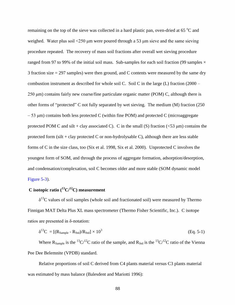
88
remaining on the top of the sieve was collected in a hard plastic pan, oven-dried at 65 oC and
weighed. Water plus soil <250 μm were poured through a 53 μm sieve and the same sieving
procedure repeated. The recovery of mass soil fractions after overall wet sieving procedure
ranged from 97 to 99% of the initial soil mass. Sub-samples for each soil fraction (99 samples ×
3 fraction size = 297 samples) were then ground, and C contents were measured by the same dry
combustion instrument as described for whole soil C. Soil C in the large (L) fraction (2000 –
250 μm) contains fairly new coarse/fine particulate organic matter (POM) C, although there is
other forms of ―protected‖ C not fully separated by wet sieving. The medium (M) fraction (250
– 53 μm) contains both less protected C (within fine POM) and protected C (microaggregate
protected POM C and silt + clay associated C). C in the small (S) fraction (<53 μm) contains the
protected form (silt + clay protected C or non-hydrolysable C), although there are less stable
forms of C in the size class, too (Six et al. 1998, Six et al. 2000). Unprotected C involves the
youngest form of SOM, and through the process of aggregate formation, adsorption/desorption,
and condensation/complexation, soil C becomes older and more stable (SOM dynamic model
Figure 5-3).
C isotopic ratio (13
C/12
C) measurement
δ13
C values of soil samples (whole soil and fractionated soil) were measured by Thermo
Finnigan MAT Delta Plus XL mass spectrometer (Thermo Fisher Scientific, Inc.). C isotope
ratios are presented in δ-notation:
δ13
C = [(RSample - RStd)/RStd] × 103 (Eq. 5-1)
Where RSample is the 13
C/12
C ratio of the sample, and RStd is the 13
C/12
C ratio of the Vienna
Pee Dee Belemnite (VPDB) standard.
Relative proportions of soil C derived from C4 plants material versus C3 plants material
was estimated by mass balance (Balesdent and Mariotti 1996):
89
C4 plants contribution = (δ - δTr) / (δCr - δTr) (Eq. 5-2)
Where δ is the δ13
C value of a given sample, δCr is the average δ13
C value of C4 plants
tissue (-13 ‰), and δTr is the average δ13
C value of C3 plants (-27 ‰). In the studied land-use
systems, trees and bushes in abandoned land are C3 plants, and crops grown underneath the
parklands around the live fence are C4 plants (sorghum and millet) as well as the presumed
previous vegetation (crops) of fodder bank and abandoned land.
Statistical Analysis
Analysis of variance (ANOVA) was used to estimate the variance components. The linear
models were applied to the soil C concentration data. Model1 was applied to all five land-use
systems, and model 2 was applied to three land-use systems (two parklands and live fence) that
have distance information. The linear models were:
Model 1: y ijkl = μ + Li + Dj + Fk + Il+ L*D ij+ L*Fik + L*Iil + D*Fjk + D*I jl + F*Ikl +
L*D*Fijk + L*D*Iijl + D*F*Ijkl + L*D*F*Iijkl + eijkl (Eq. 5-3)
Model 2: y ijklm = μ + Li + Dj + Fk + Il + Tm+ L*D ij+ L*Fik + L*Iil + D*Fjk + D*I jl + F*Ikl
+ L*T im + D*Tjm + F*Tkm + I*Tlm + L*D*Fijk + L*D*Iijl + D*F*Ijkl + L*D*T ijm+
L*F*Tikm + L*I*Tilm + D*F*Tjkm + D*I*T jlm + F*I*Tklm + L*D*F*Iijkl + L*D*F*Tijkm +
L*D*I*Tijlm + D*F*I*Tjklm + L*D*F*I*Tijklm+ eijklm (Eq. 5-4)
y ijklm is the C concentration in land-use i, at depth of j, fraction size of k, isotopic ratio of l,
distance of m.
μ is the population mean,
Li is the land-use (treatments), i = FA, VP, LF, FB, and AL.
FA: F. albida parkland, VP: V. paradoxa parkland, LF: live fence, FB: fodder bank, and
AL: abandoned land.
Dj is the depth, j = 1 – 3
90
1: 0 – 10 cm, 2: 10 – 40 cm, 3: 40 – 100 cm.
Fk is the fraction size, k = L, M, S
L: large fraction (2000 – 250 μm), M: medium fraction (250 – 53 μm), S: small fraction
(<53 μm)
Il is the isotopic ratio, l = C3, C4
C3: C3 plants origin C, C4: C4 plants origin C
Tm is the distance, m = n, m, f
n: near the tree, m: middle of the canopy, f: far from the tree
eijklm is the random variable error within the experiment.
Model 1 and model 2 including all the possible interactions between the factors were run
using PROC MIXED procedure of SAS. Interactions that were not significant were dropped
from the model. The models that were biologically and statistically significant are presented in
the results section. To further examine the interactions, data were sorted (PROC SORT
procedure) with certain factors fixed, and tested again using ANOVA. Based on the outcome of
the ANOVA, factors and other soil characteristics (e.g. percentage of sand, silt, and clay) were
tested for their relationships using linear regression.
All statistical tests were considered significant when p<0.05 unless otherwise specified.
Results
Soil Characteristics
Soils in the sample plots are mostly sandy loam or loamy sand (Table 5-1). Soil colors
varied from whitish or dark gray to reddish brown in different plots, but all are categorized as
Haplustalfs by the regional survey (Doumbia 2000). Abandoned-land soil was extremely hard to
sample with an auger because bedrock was found in some places at less than 1 m depth (Figure
5-2). Most of the time, silt or clay was clearly observed in 70 – 80 cm depths. Content (g kg-1
91
soil) of sand, silt and clay were compared statistically over the five land-use systems.
Abandoned land had lower sand content (530 – 694 g kg-1
soil) and higher content of silt and
clay (306 – 470 g kg-1
soil) than the other four systems (sand: 715 – 935 g kg-1
soil, silt + clay:
65 – 285 g kg-1
soil) (Table 5-1). Soils of the four systems in each depth class were not different
in the particle size content.
Whole Soil C
Whole soil C content across all the systems varied from 1 – 6 g C kg-1
soil (Figure 5-4).
Two parklands and live fence had three sampling locations (0, 3, and 10 m from tree base for
parklands; 0, 1, and 3 m from tree lines for live fence). Only the surface soil (0 – 10 cm) of live
fence showed a difference between the ―near tree‖ and the two zones more distant from the tree,
but other depth classes and two parklands plots did not show difference by horizontal distance
from trees, although the trend of ―near tree‖ > ―outside crown‖ was observed in the surface soil
of both parkland systems. C content decreased with soil depth for all land-use systems except
the fodder bank, where the surface soil (0 – 10 cm) had less whole soil C than lower depths.
The whole soil C data of five land-use systems were compared statistically using two
factorial (land-use and depth) ANOVA (model 1). Both land-use and depth factors, as well as
land-use*depth interaction were significant for that variables. By Tukey-Kramer multiple
comparison test, abandoned land had higher C content than the other four systems, but the other
four systems were not different from each other. C content was different by depth: 0 – 10 cm >
10 – 40 cm > 40 – 100 cm across all treatments.
Among the data for the two parklands and live fence plots, horizontal distance was another
―factor‖ (model 2). Land-use and depth factors were significant, but distance was not
significant, although showing the trend (p=0.0884), in the three-way factorial (land-use, depth,
and distance) ANOVA. When land-use factor and distance factor were examined in the fixed
92
depth class, the distance factor was still not significant in any depth class. However, at 10 – 40
cm and 40 – 100 cm classes, C content was higher for F. albida parkland than in the case of the
live fence.
C in Soil Fractions
Carbon-fraction contents [large (L): (250 – 2000 μm), and medium (M): (53 – 250 μm)] in
different systems were mostly not different among each other, and ranged from 1 to 2 g C kg-1
soil (except in fodder bank, where it was from 0 to 1 C kg-1
soil) (Figure 5-5). Small (S) fraction
(<53 μm) C content did not change much from 0 – 10 cm to 10 – 40 cm depth in all systems. In
the live fence treatment, C in the 0 – 10 cm depth contained more L fraction (1.8 g C kg-1
soil)
than the other two size fractions (less than 0.7 g C kg-1
soil), whereas the fodder bank treatment
had very low C content of L and M fractions in that soil layer (0.6 g C kg-1
soil).
Data of C in the three fractions were analyzed by three-factorial ANOVA (land-use, depth,
and size) (model 1). All three factors were significant, as well as three combinations of two-
factor interactions. Results of multiple comparisons among land-use systems were the same as
for the whole soil C data; abandoned land had higher C content than the other four systems,
which did not differ among each other. Depth class comparison also showed the same result: 0 –
10 cm > 10 – 40 cm > 40 – 100 cm. S fraction and L fraction C were both significantly higher in
content than M fraction C when three depth class data are combined. The significance varied
when each depth class was separately tested, but M fraction C content was always the lowest.
When each fraction size data were tested separately, land-use and depth were significant for all
fraction sizes.
Distance from the tree was the only factor that was not significant in four-factorial
ANOVA (land-use, depth, size, and distance) for three systems (two parklands and live fence:
model 2). Interactions of four factors and three factors including distance were not significant.
93
Further sorting and testing showed that the distance factor was significant in only M fraction C at
the 0 – 10 cm depth, where ―near tree‖ was higher in content than ―outside crown.‖
Isotope Analysis of Whole Soil C
The measured δ13
C values of each depth class of each land-use systems varied from –23.9
to –15.1 (Table 5-2). Based on the values and the mass balance calculation, whole soil C data
was separated into that originating from C3 plants (trees) and C4 plants (crops) (Figure 5-6).
―Near tree‖ data and ―outside crown‖ data are presented side by side for two parklands (Figure 5-
6 A, B, C, D) and live fence (Figure 5-6, E, F). In the figure, C of tree origin was found more in
surface soil and near the tree, although when they were tested statistically, there was no
significant difference between ―near tree‖ and ―outside crown‖ data except for that of live fence
at the 0 – 10 cm depth. Fodder bank did not have much C of C3-origin, even with trees growing
in the plots. On abandoned land, C4-origin C was the major form of C, and, as mentioned
earlier, the soil C content was higher in this system compared with other systems.
Three-factorial (land-use, depth, and isotopic ratio) ANOVA was conducted among the
five land-use systems (model 1). All factors were significant, and three-factor interaction and
two-factor interactions including isotopic ratio were also significant. C3-origin C and C4-origin
C were then tested separately using the ―SORT‖ procedure. Land-use was not a significant
factor among C3-origin C data, but depth was. For C4-origin C, both land-use and depth had
significant effect: abandoned land had higher content than other four systems with parklands
higher than the improved systems, and deeper depth had less C content.
Four-factorial (land-use, depth, distance, and isotopic ratio) ANOVA was used to test
differences among the two parklands and live fence systems (model 2). Distance was again not a
significant factor while all others were. Four-factor interaction, as well as three- and two-factor
interactions including distance was significant, suggesting distance was somewhat influential for
94
C content. When only C3-origin C data was tested separately, land-use was not significant but
depth and distance were. Multiple comparison tests showed that C3-origin C content from ―near
tree‖ and ―half crown‖ were higher than that from ―outside crown‖ throughout the three systems.
Among C4-origin C, land-use and depth were significant factors but distance was not.
Isotope Analysis of C in Soil Fractions
The measured δ13
C values of three fraction sizes varied from –25.4 to –15.7 (Table 5-2).
Data of C content in the three size fractions were also separated into those with C originating
from C3 and C4 plants (Figure 5-7). Four-factorial ANOVA (land-use, depth, size, isotopic
ratio) was used to test differences among the five land-use systems (model 1). Land-use, depth,
and size were significant factors, but isotopic ratio was not. Four-factor interaction was not
significant, but all two-factor interaction combinations including isotopic ratio were significant
(p<0.01). When C3-origin C was tested separately, land-use was not significant while size and
depth were. All three were significant factors among C4-origin C data. When data were sorted
by the fraction size, C3-origin C was significantly more than C4-origin C in the L fraction, while
C4-origin C was more than C3-origin C in the S fraction.
Among the two parklands and live fence data sets, five-factorial ANOVA (land-use, depth,
size, isotopic ratio, and distance) was conducted (model 2). Land-use, size and depth were
significant, but isotopic ratio and distance were not. All combinations of three-factor
interactions including isotopic ratio and distance were significant, so was the two-factor
interaction of distance and isotopic ratio. Distance became a significant factor (―near tree‖ >
―outside crown‖) for C3-origin C data sets, while it was not for C4-origin C.
Relationships of Data Sets
Linear relationships were tested between C content data sets and other soil characteristics
of the samples. The S fraction (<53 μm) percentage in whole soil had significant relationship
95
(R2=0.60) with the S size C (contains protected C) content. However, this relationship was not
seen for M and L fractions; the more fraction percentage of M or L size in the soil does not mean
the more soil C of those sizes. Also, the regression between silt + clay content and whole soil C
content was strong, especially in the 10 – 40 cm soil depth (Figure 5-8).
Sand-, silt-, clay-, or silt + clay contents did not have strong relationship with L fraction C
or M fraction C. Although the regression between silt + clay content and S fraction C was poor
(R2=0.16) in the total data set, it became more pronounced when the data set was divided by
depth class. R2
values between silt + clay and S fraction C were 0.53 at 0 – 10 cm, 0.44 at 10 –
40 cm, and 0.67 at 40 – 100 cm (Figure 5-9). Soil pH or bulk density did not show any strong
relationship with C in whole soil or in each of the three fractions in any depth or for all depths
combined.
Percentages of C3-origin C or C4-origin C did not have a significant relationship with
whole soil C content. There was a strong relationship between C3-origin C content and L
fraction C content (R2=0.67) throughout the data set. The relationship was stronger at 0 – 10 cm
soil (R2=0.72) when data sets were divided by depth (Figure 5-10), but were not significant in
deeper depths. The relationship between C3-origin C and S fraction C content was also observed
in the 40 – 100 cm depth (R2=0.45).
Discussion
Contrary to expectations, C content in all soil depths was higher in the ―abandoned‖ land
than in any of the four agroforestry systems (Figure 5-4), although the significance varied
depending on the depth class. Judging from the observation that the abandoned land soil had
significantly more silt and clay fractions than those of soils under the agroforestry systems
(Table 5-1), it seems that the whole soil C content was directly related to the silt and clay
contents of the soil. In general, soil organic C content is known to correlate positively with the
96
amount of non-crystalline clays (Powers and Schlesinger 2002). Indeed, the whole soil C
content was related to silt + clay content in all three depth classes (strongest in 10 – 40 cm)
(Figure 5-8). Silt + clay content also had strong relationship with S fraction C (<53 μm), the
strongest being in 40 – 100 cm (Figure 5-9), but not as well as with whole soil C. This suggests
that silt and clay are mainly associated with soil C in <53 μm size, especially in deep soil, but
they are also associated with larger fraction size form of soil C. Based on the data points on
Figure 5-9, abandoned land data do not seem to follow this relationship well, while they follow
the relationship better in Figure 5-8. This could be because silt and clay are more involved in
forming larger than 53 μm fraction size C in abandoned land compared with other systems.
After being abandoned for a few years (less than 10: see Chapter 4), the land probably was
subjected to extensive erosion that took away aggregates and sandy particles from the surface
layer. The remaining soil was higher in silt and clay and formed a hard surface pan, which
prevented further disturbance or leaching. The majority of soil C in the abandoned land was of
C4 plant origin (Figure 5-6), suggesting that the stored C in abandoned land was mainly from the
previous land-use (land cultivated with C4 plants) and was well protected.
The other four land-use systems were not significantly different in terms of the soil
characteristics (pH, bulk density, particle size). However, as seen in the soil pit photo (Figure 5-
2), the color was quite different in each soil pit, suggesting soil variations among plots of same
land-use systems in the same village. Still, soil C content variations among these soils can be
explained more as a consequence of the influence of trees and land management than caused by
soil characteristics as in the case of abandoned land. Among the two parklands and live fence
systems, C content was expected to be: near tree > under the crown > outside the crown, as
reported in a similar study in the parkland system in South Mali, which showed the significant
97
difference between near tree and outside the crown in 0 – 20 cm (although not significant in 20 –
40 cm) (Kater et al. 1992). However, in this study, the tree effect (distance factor) was only
significant in the live fence but not in the two parkland systems (the trends of ―near tree‖ >
―outside crown‖ were observed in both parklands) (Figure 5-4). From the field observation, this
seems to be because of the frequent tillage (a couple of times during the growing season) in the
parklands. Many studies reported that tillage caused significant loss of soil organic C especially
in the surface (Gebhart et al. 1994; Campbell et al. 1996; Six et al. 1998). Tillage using animal
traction is done very close to the trunks of parkland trees where tree density is low, and this
accelerates the decomposition of organic matter in the top soil, and thus reduces soil C
accumulation. Live fence trees are planted in high density and their thorny branches spread,
making it almost impossible to do tillage near the tree lines. C content around the live fence tree
lines is higher due to the higher litter inputs from trees (Figure 5-6). The positive correlation of
C3 (tree)-derived C and L fraction (contains new SOM) C in the 0 – 10 cm soil (Figure 5-10)
also suggests that the recent planting of live fence trees and the input of litter have already
contributed to the accumulation of C in the topsoil.
The reason why fodder bank systems did not have much topsoil C (Figure 5-4) could also
be explained by the management style. First, the land is tilled before planting the trees, which
causes the loss of aggregated C (L and M fraction C). Then, crops are not grown inside the
fodder bank after tree planting, and most of the tree leaves and branches are taken away as
fodder. The low litter input after establishment also causes the low density of L and M fraction
C (Figure 5-5). Since S fraction C contains well-protected C, its content in fodder banks was not
affected much by the tillage, and stayed similar with other systems in all depths.
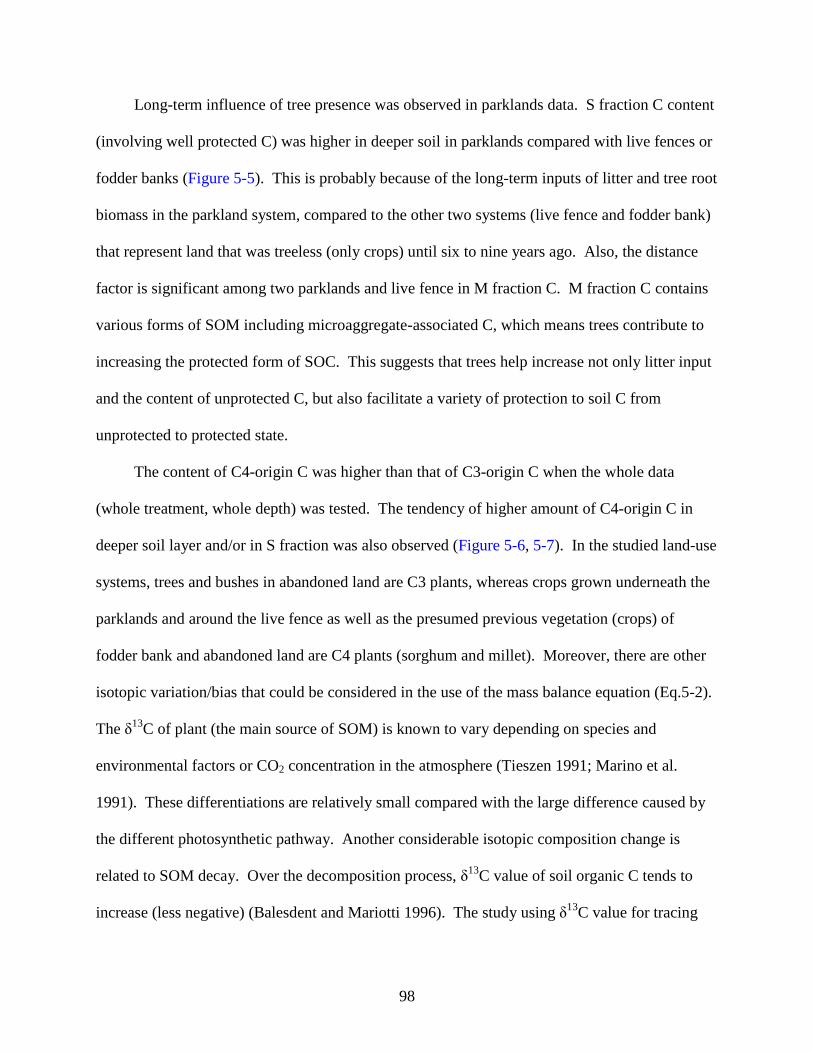
98
Long-term influence of tree presence was observed in parklands data. S fraction C content
(involving well protected C) was higher in deeper soil in parklands compared with live fences or
fodder banks (Figure 5-5). This is probably because of the long-term inputs of litter and tree root
biomass in the parkland system, compared to the other two systems (live fence and fodder bank)
that represent land that was treeless (only crops) until six to nine years ago. Also, the distance
factor is significant among two parklands and live fence in M fraction C. M fraction C contains
various forms of SOM including microaggregate-associated C, which means trees contribute to
increasing the protected form of SOC. This suggests that trees help increase not only litter input
and the content of unprotected C, but also facilitate a variety of protection to soil C from
unprotected to protected state.
The content of C4-origin C was higher than that of C3-origin C when the whole data
(whole treatment, whole depth) was tested. The tendency of higher amount of C4-origin C in
deeper soil layer and/or in S fraction was also observed (Figure 5-6, 5-7). In the studied land-use
systems, trees and bushes in abandoned land are C3 plants, whereas crops grown underneath the
parklands and around the live fence as well as the presumed previous vegetation (crops) of
fodder bank and abandoned land are C4 plants (sorghum and millet). Moreover, there are other
isotopic variation/bias that could be considered in the use of the mass balance equation (Eq.5-2).
The δ13
C of plant (the main source of SOM) is known to vary depending on species and
environmental factors or CO2 concentration in the atmosphere (Tieszen 1991; Marino et al.
1991). These differentiations are relatively small compared with the large difference caused by
the different photosynthetic pathway. Another considerable isotopic composition change is
related to SOM decay. Over the decomposition process, δ13
C value of soil organic C tends to
increase (less negative) (Balesdent and Mariotti 1996). The study using δ13
C value for tracing
99
the vegetation change in East African savannah suggests that using the mass balance approach to
interpret soil profiles might lead to an under-estimation of past C3 plant abundance (Gillson et al.
2004). Thus, the C3-origin C, especially in deeper soil tends to be underestimated, and this
might be one of the reasons that C3-origin C in the deeper soil (tree root contribution) was not
observed as much as expected. It is also probably due to the higher inputs of belowground
biomass from crops in the sampling depth. Aboveground crop residue is usually taken away as
fodder in fodder bank, but crop roots are annually left in the soil and become the source of soil
organic C. Crop roots are also expected to have a faster decomposition rate than tree roots that
contain higher proportion of lignin and other substances that slow down the decomposition
process. In addition, sampling depth (1 m) might not be enough to see more tree roots influence
than crop roots influence. Most of Mali‘s soil research sets 40 cm as the crop root influence
limit, but a study found a significant amount of sorghum roots close to or deeper than 60cm in a
similar climatic condition (Jones et al. 1998). Tree roots, especially in semiarid areas, are
expected to go even deeper than 1 m (Jeltsch et al. 1996).
Overall, soil organic C content in the studied systems were of relatively lower magnitude
(1 to 6 g C kg-1
soil), than in agriculture or agroforestry systems of other ecoregions. This is
possibly due, at least partly, to the rapid decomposition of organic C, which is known to be
facilitated by the high temperature and low silt and clay contents (Schimel et al. 1994; Hassink
1997). The lower amount of M fraction C than S and L fraction C (when tested with all
treatments data combined) also suggests that most of the litter inputs are decomposed rapidly so
that little is going to the process of becoming a more protected form of C. In many situations, it
is probably best for farmers to allow the majority of the residues to be eaten by cattle in these
systems rather than attempt to build soil organic matter.
100
A conservative estimate of soil C sequestration potential through addition of organic
matter such as plant litter and animal waste to these agricultural soils is in the range of 0.1 – 0.3
Mg C ha-1
yr-1
(Batjes 2004). ICRAF is trying to promote live fences and fodder banks for land
amelioration and counts C sequestration potential as one of the potential benefits. However, it is
important to address the possibility of causing net loss of soil C while converting abandoned land
into live fences or fodder banks in this study region at the initial stage, because of the tillage
factor at establishment. And, because the subsequent land-use practices provide low levels of
litter input, especially in fodder banks, it may take a long time to regain the initial loss of soil C.
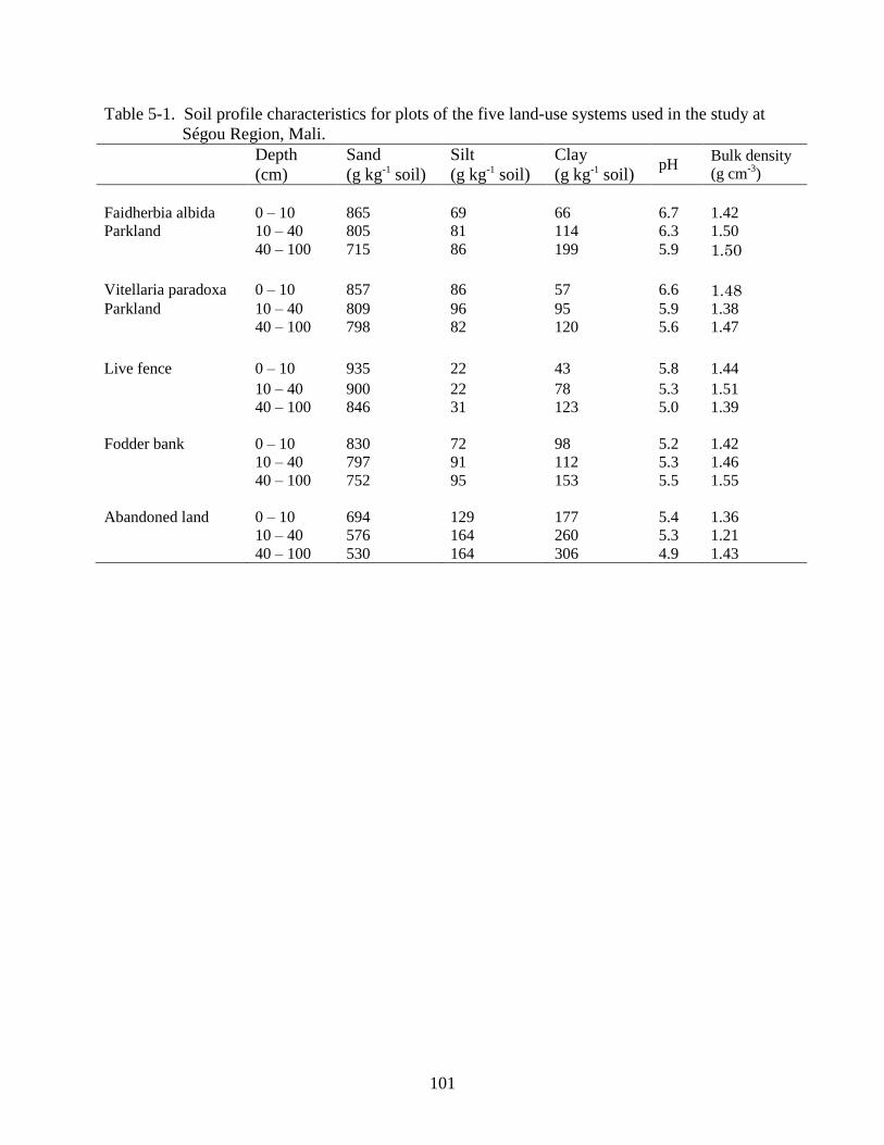
101
Table 5-1. Soil profile characteristics for plots of the five land-use systems used in the study at
Ségou Region, Mali.
Depth
(cm)
Sand
(g kg-1 soil)
Silt
(g kg-1 soil)
Clay
(g kg-1 soil) pH
Bulk density
(g cm-3
)
Faidherbia albida
0 – 10
865
69
66
6.7
1.42
Parkland 10 – 40 805 81 114 6.3 1.50
40 – 100 715 86 199 5.9 1.50
Vitellaria paradoxa
0 – 10
857
86
57
6.6
1.48 Parkland 10 – 40 809 96 95 5.9 1.38
40 – 100 798 82 120 5.6 1.47
Live fence
0 – 10
935
22
43
5.8
1.44
10 – 40 900 22 78 5.3 1.51
40 – 100 846 31 123 5.0 1.39
Fodder bank
0 – 10
830
72
98
5.2
1.42
10 – 40 797 91 112 5.3 1.46
40 – 100 752 95 153 5.5 1.55
Abandoned land
0 – 10
694
129
177
5.4
1.36
10 – 40 576 164 260 5.3 1.21
40 – 100 530 164 306 4.9 1.43

102
Table 5-2. δ13
C values of whole soil and three fraction sizes from five studied land-use systems,
at Ségou Region, Mali. (all values are average of three replicates)
Whole soil Fraction
Land-use system Depth (cm) 250 – 2000 µm 53 – 250 µm <53 µm
Faidherbia albida near tree 0 – 10 -21.5 -22.4 -20.3 -21.2
parkland 10 – 40 -18.7 -20.3 -20.2 -18.6
40 – 100 -16.6 -18.8 -18.6 -18.1
3 m from tree 0 – 10 -21.8 -22.9 -21.8 -21.5
10 – 40 -17.5 -20.7 -19.7 -18.3
40 – 100 -15.6 -18.2 -17.2 -17.3
10 m from tree 0 – 10 -19.5 -20.9 -20.0 -19.3
10 – 40 -16.9 -21.4 -20.6 -17.3
40 – 100 -15.1 -20.0 -18.6 -15.9
Vitellaria paradoxa near tree 0 – 10 -20.7 -23.1 -21.1 -21.4
parkland 10 – 40 -18.8 -23.3 -20.1 -20.1
40 – 100 -18.7 -22.7 -20.8 -19.2
3 m from tree 0 – 10 -20.6 -22.7 -20.4 -20.6
10 – 40 -17.8 -19.9 -18.3 -17.8
40 – 100 -17.8 -20.9 -18.8 -18.3
10 m from tree 0 – 10 -18.7 -20.5 -18.1 -19.3
10 – 40 -17.6 -19.2 -18.9 -19.0
40 – 100 -16.8 -19.6 -20.8 -18.9
Live fence near tree 0 – 10 -23.9 -25.4 -23.9 -22.6
10 – 40 -20.1 -21.1 -19.8 -20.3
40 – 100 -17.1 -19.2 -18.0 -17.7
1 m from tree line 0 – 10 -22.5 -23.3 -22.4 -23.1
10 – 40 -19.3 -22.2 -19.3 -18.8
40 – 100 -16.9 -19.2 -18.6 -17.7
3 m from tree line 0 – 10 -20.9 -22.2 -18.8 -20.8
10 – 40 -17.9 -18.9 -19.1 -17.7
40 – 100 -16.3 -19.7 -18.9 -16.8
Fodder bank 0 – 10 -18.2 -20.4 -21.2 -19.1
10 – 40 -17.9 -21.3 -20.4 -17.4
40 – 100 -17.4 -22.9 -18.7 -16.9
Abandoned land 0 – 10 -16.3 -16.8 -18.5 -16.4
10 – 40 -15.7 -16.9 -16.5 -15.7
40 – 100 -16.4 -18.0 -16.2 -16.8
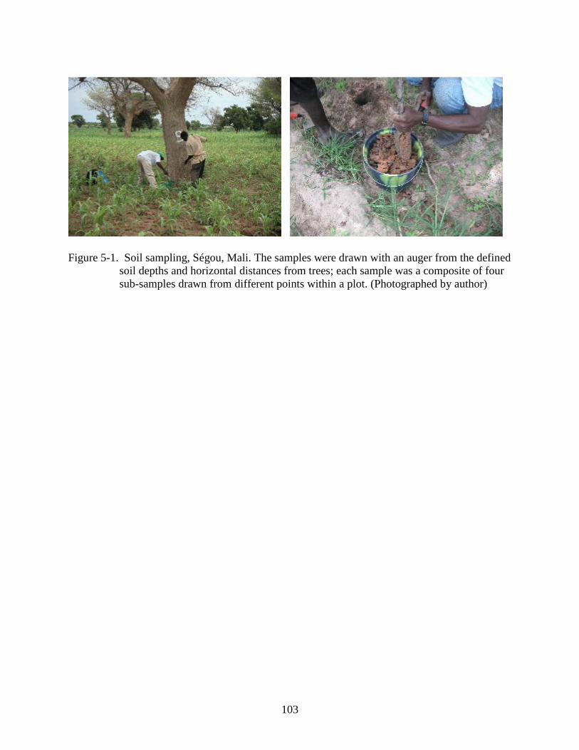
103
Figure 5-1. Soil sampling, Ségou, Mali. The samples were drawn with an auger from the defined
soil depths and horizontal distances from trees; each sample was a composite of four
sub-samples drawn from different points within a plot. (Photographed by author)
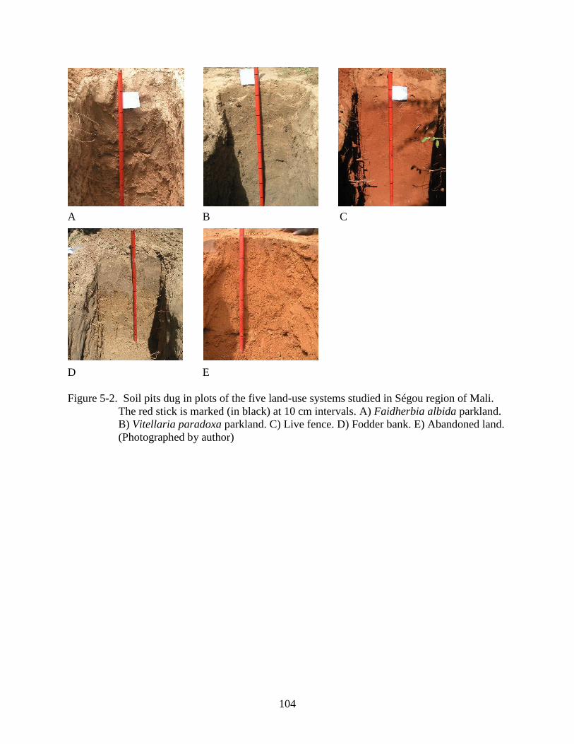
104
A B C
D E
Figure 5-2. Soil pits dug in plots of the five land-use systems studied in Ségou region of Mali.
The red stick is marked (in black) at 10 cm intervals. A) Faidherbia albida parkland.
B) Vitellaria paradoxa parkland. C) Live fence. D) Fodder bank. E) Abandoned land.
(Photographed by author)
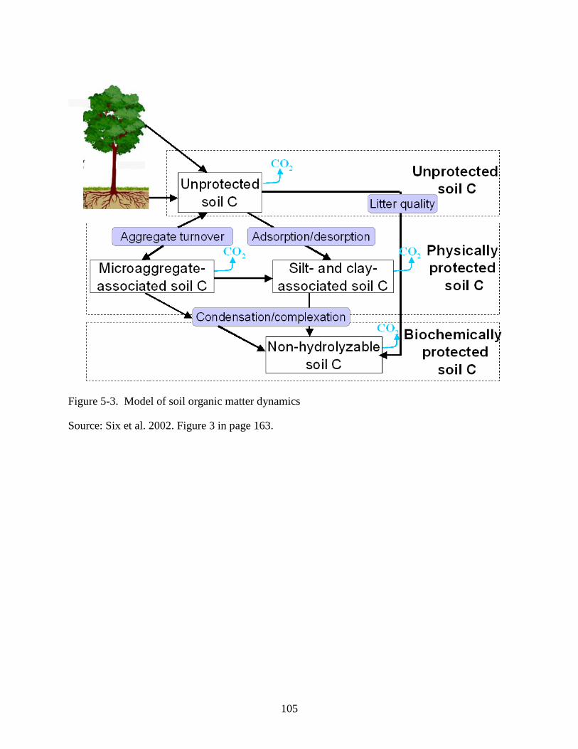
105
Figure 5-3. Model of soil organic matter dynamics
Source: Six et al. 2002. Figure 3 in page 163.
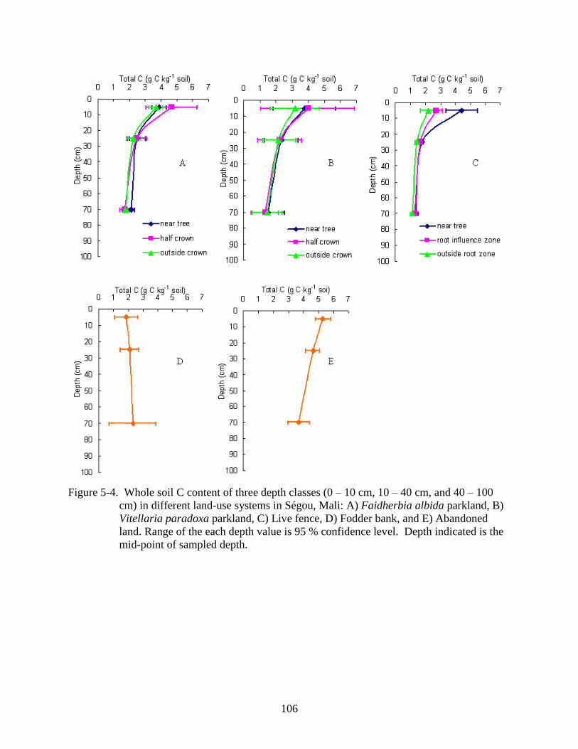
106
Figure 5-4. Whole soil C content of three depth classes (0 – 10 cm, 10 – 40 cm, and 40 – 100
cm) in different land-use systems in Ségou, Mali: A) Faidherbia albida parkland, B)
Vitellaria paradoxa parkland, C) Live fence, D) Fodder bank, and E) Abandoned
land. Range of the each depth value is 95 % confidence level. Depth indicated is the
mid-point of sampled depth.
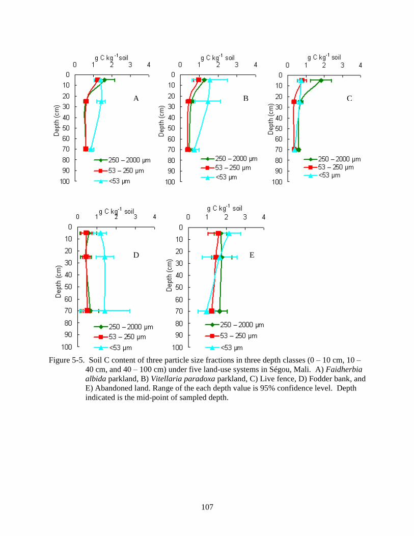
107
Figure 5-5. Soil C content of three particle size fractions in three depth classes (0 – 10 cm, 10 –
40 cm, and 40 – 100 cm) under five land-use systems in Ségou, Mali. A) Faidherbia
albida parkland, B) Vitellaria paradoxa parkland, C) Live fence, D) Fodder bank, and
E) Abandoned land. Range of the each depth value is 95% confidence level. Depth
indicated is the mid-point of sampled depth.
D E
A B C
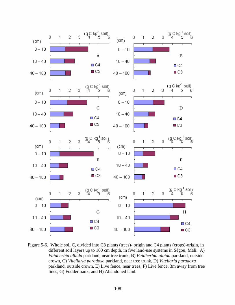
108
Figure 5-6. Whole soil C, divided into C3 plants (trees)- origin and C4 plants (crops)-origin, in
different soil layers up to 100 cm depth, in five land-use systems in Ségou, Mali. A)
Faidherbia albida parkland, near tree trunk, B) Faidherbia albida parkland, outside
crown, C) Vitellaria paradoxa parkland, near tree trunk, D) Vitellaria paradoxa
parkland, outside crown, E) Live fence, near trees, F) Live fence, 3m away from tree
lines, G) Fodder bank, and H) Abandoned land.
A B
C D
D
D
E
D
D
F
D
D
G
D
D
H
D
D
109
Figure 5-7. Soil C in three fraction sizes divided into C3 plants-origin and C4 plants-origin in
different soil particle-size fractions under different land-use systems in Ségou, Mali.
A) Faidherbia albida parkland, near tree trunk, B) Faidherbia albida parkland,
outside crown, C) Vitellaria paradoxa parkland, near tree trunk, D) Vitellaria
paradoxa parkland, outside crown, E) Live fence, near trees, F) Live fence, 3m away
from tree lines, G) Fodder bank, and H) Abandoned land.
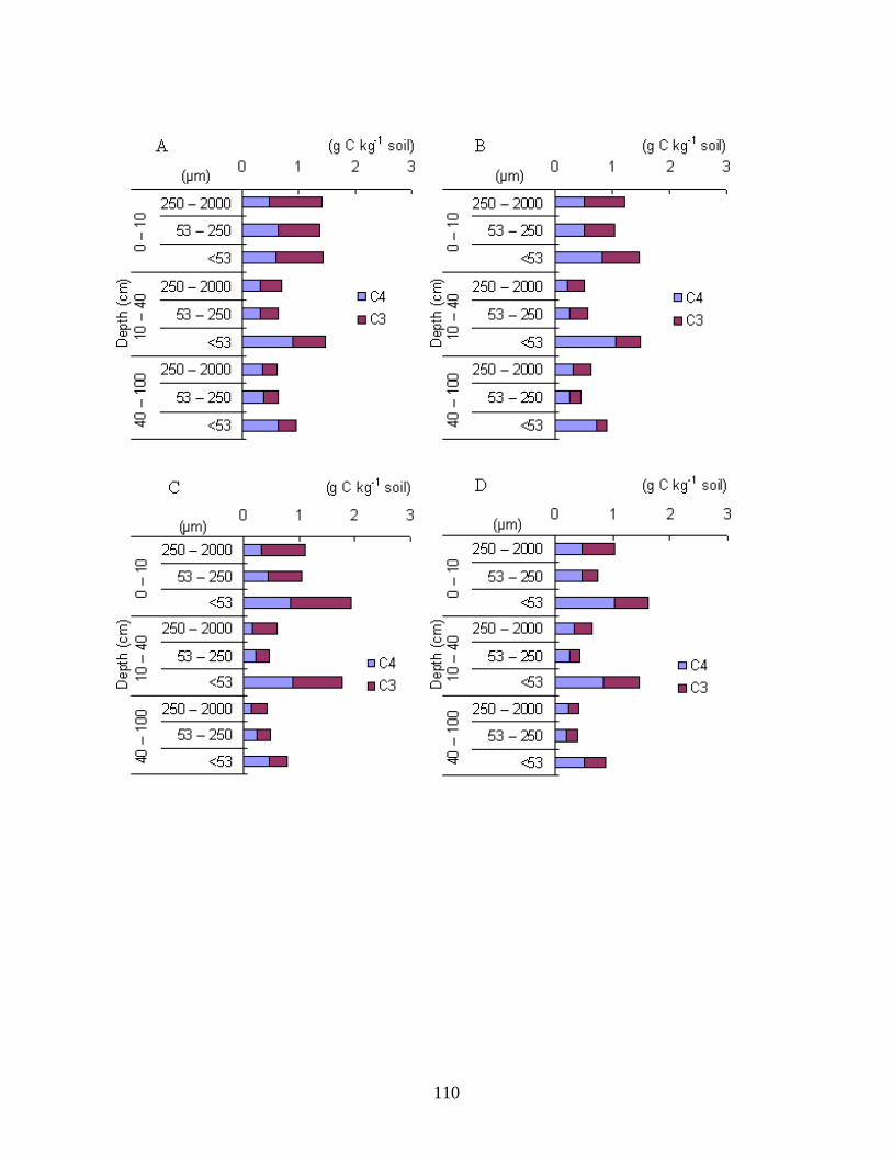
110
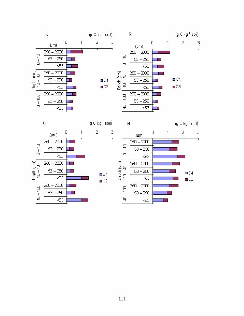
111
112
Figure 5-8. Linear regression between silt + clay content of soil and whole soil C content in
three depth classes across five land-use systems in Ségou region of Mali. The three
data points, one each in each depth class, marked by circles around them, refer to one
of the fodder bank plots the data from which were quite inconsistent with those from
the other fodder bank plots as well as all the other treatments; these points were
therefore considered as outliers and excluded from the regression.
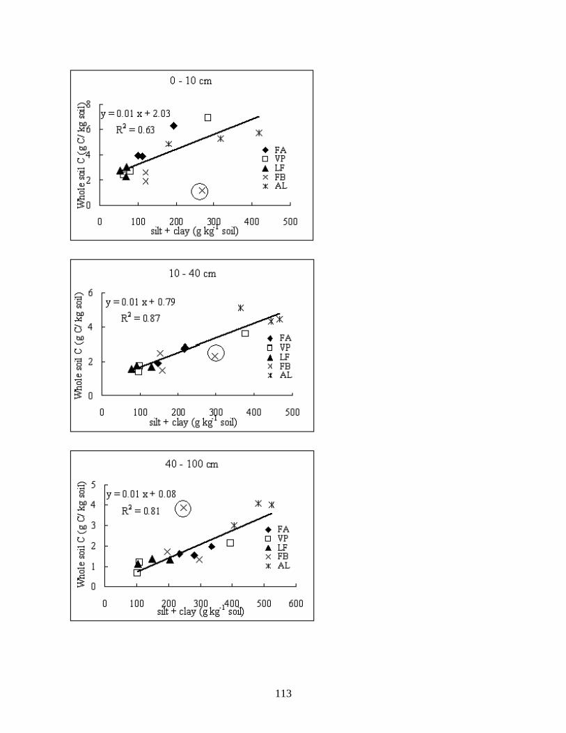
113
114
Figure 5-9. Linear regression between silt and clay content of soil and C in soil particles of <53
μm in three soil-depth classes across five land-use systems in Ségou, Mali. The three
data points, one each in each depth class, marked by circles around them, refer to one
of the fodder bank plots the data from which were quite inconsistent with those from
the other fodder bank plots as well as all the other treatments; these points were
therefore considered as outliers and excluded from the regression.
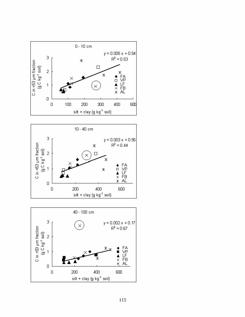
115
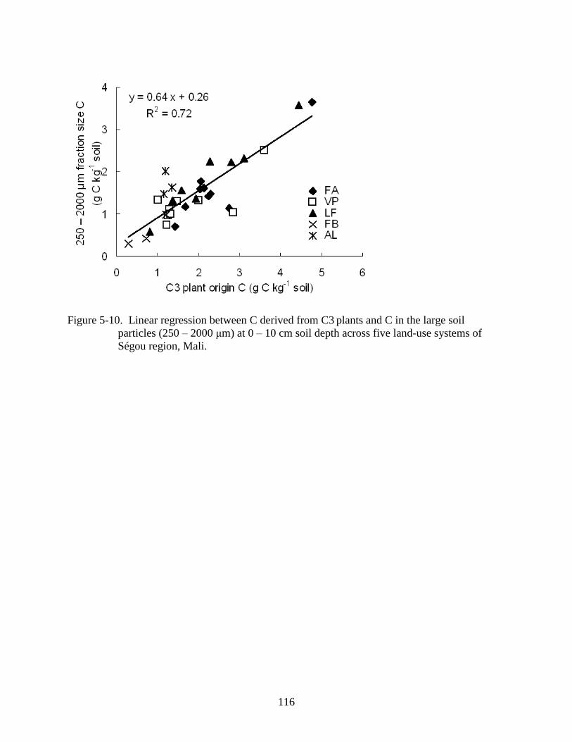
116
Figure 5-10. Linear regression between C derived from C3 plants and C in the large soil
particles (250 – 2000 μm) at 0 – 10 cm soil depth across five land-use systems of
Ségou region, Mali.
117
CHAPTER 6
SOCIOECONOMIC ANALYSIS OF THE CARBON SEQUESTRATION POTENTIAL OF
IMPROVED AGROFORESTRY SYSTEMS IN MALI, WEST AFRICA
Introduction
The success in the implementation of any project for greenhouse gas (GHG) mitigation
through agricultural means will depend on the farmers‘ willingness to participate in the project.
This is particularly so in a region such as this study site where the vast majority of inhabitants
rely on the outputs from their crop fields and animals for subsistence and cash income rarely
exists in their household budgets. These farmers might be encouraged to plant trees in their
croplands for potential carbon (C) benefits (cash payments), considering that agroforestry is a
recognized GHG mitigation strategy according to the Kyoto Protocol. Several major reasons
have been recognized as favoring introduction of C sequestration benefits into smallholders‘
agroforestry practices in developing countries. One is that this sequestration service does not
need to be transported, thus, it can benefit people in remote areas, many of whom are poor.
Secondly, there are no quality differences: a molecule of C is the same wherever it is located; so
the problem often faced by smallholders in not being able to achieve the quality required by
international markets in agricultural commodities does not apply here (Cacho et al. 2003a).
Furthermore, even small amounts of additional income would make a great difference for these
subsistence farmers who have practically no opportunity to make such additional cash income.
The political environment is also favorable for enhancing smallholders‘ involvement in
GHG mitigation projects. The United Nations Framework Convention on Climate Change
(UNFCCC) included development, equity, and sustainability as conditions to be met when
setting its principles for stabilizing GHG concentrations through mitigation policy (UNFCCC
2007). Large-scale adoption of C sequestration activities by agroforestry in African countries
could contribute to these objectives through biodiversity conservation, rural employment, and
118
soil amelioration (Breman 1997; Tschakert 2007). The World Agroforestry Centre (ICRAF)
announced that they were confident that establishment of agroforestry, especially in degraded
land, would qualify and play an important role under the Clean Development Mechanism (CDM)
of Kyoto Protocol (ICRAF 2007).
A few major problems exist, however, in the context of promoting agroforestry practices
by smallholders for entering CDM market. For example, we need to examine cost per unit of C
sequestration since there are many other options such as emission reduction or sequestration by
large-scale monoculture plantation (De Jong et al. 2004). Furthermore, based on the feasibility
studies, appropriate technical and political assistance should be provided so that smallholder of
agroforestry owners will not always be less competitive than other mitigation projects options.
Thus, socioeconomic feasibility of the improved systems is an important consideration in the
context of agroforestry implementation for GHG mitigation, and that is the scope of this chapter.
Under the Kyoto Protocol, only newly sequestered C as a result of the project is
recognized as ―tradable‖ C; the traditional agroforestry systems such as parklands are, thus, not
likely to be counted as C sequestration projects. The improved agroforestry systems that are
currently being introduced in the study region can be qualified for tradable C credits. Therefore,
the target agroforestry systems for this study are live fence and fodder bank in Ségou region,
Mali (detailed system description in Chapter 4).
Research Questions
1. What is the relative attractiveness of the two improved agroforestry systems (live fence and
fodder bank) considering their C sequestration potential, economic profitability, and social
acceptability?
2. If C credit markets were introduced under the CDM of Kyoto Protocol, would adoption of
agroforestry provide more profits to land owners? If yes, how much?
119
Materials and Methods
The World Agroforesty Centre (ICRAF) conducted monitoring surveys for farmers
implementing live fences and fodder banks after introduction of the systems (Hamer et al. 2005,
van Duijl 2000). Data from these studies as well as databases from ICRAF research station were
used for this study. Furthermore, field surveys were conducted during February – March 2006
(the dry season after the harvests when farmers were less busy with agricultural activities) to
collect additional data necessary for the analysis.
The target population was composed of farmers living in the Ségou region who had
adopted live fences and/or fodder banks with assistance of ICRAF. A comprehensive cost-
benefit study of live fences had already been conducted for ICRAF by van Dorp et al. (2005).
Also, the need and social acceptability of live fences and fodder banks had been discussed in
several previous studies (van Duijl 1999; Levasseur 2003; Yossi et al. 2005). The information
about the fodder bank implementation was much more scarce than that of live fence. Thus, the
survey focused on collecting more data for fodder banks, specifically data to conduct the cost-
benefit analysis (CBA) equivalent to the existing live fence study, as well as data such as the
price of timber and non-timber products from both live fences and fodder banks to conduct risk
simulation analysis.
Social Survey of Fodder Bank Farmers
The questionnaire was designed based on that of the live fence survey (Annex A),
following the protocol of the Institutional Review Board of University of Florida (Protocol #
2005-U-1023). The structured questionnaire consisted of open-ended and/or close-ended
questions of 14 sections, asking for information about materials and labor used for managing and
harvesting fodder banks as well as related benefits from the implementation.
120
Twenty-two farmers from 13 different villages in the Ségou region were interviewed (the
live fence survey was conducted on 18 owners from 15 different villages). The language used
was Bambara, the most common local language in Mali, although the questionnaire was made in
French. A translator (French – Bambara), an agronomist who had conducted social survey for
ICRAF, was hired to communicate with interviewees (Figure 6-1). To ensure his
survey/interviewing skill, an experienced ICRAF officer went through the survey questionnaire
with him before the real survey started, and made him practice the follow-up explanations in case
farmers did not understand the questions.
The majority of fodder banks were 0.25 ha (50 m * 50 m) in area, since that was the
default recommendation of ICRAF. Some interviewed farmers turned out to have larger or
smaller sizes by the time of the survey, due to the success or failure of the management. All the
labor data and other costs were converted to per 0.25 ha basis before taking the mean. The live
fence study was based on the average live fence row-length, 291 m (van Dorp et al. 2005).
Because the live fence and/or fodder bank installation was at least a couple of years ago,
farmers seemed to have difficulties recalling the installation costs, especially labor (days and
people) needed for planting and management. Also, it was very difficult to estimate the amounts
of products harvested such as fodder and fruits. The sizes of the bags farmers were using to
collect the harvests varied. Direct measurements of the bag size and the fodder weight (air-
dried) were conducted at several villages to reduce the estimation variability.
Local Market Survey
There are three local markets inside the city of Ségou where most of the farmers in the
villages go to buy/sell their products and equipment. Price data were collected from all markets,
although some products such as fodder were not sold in all the markets. The average price of
each item was used for the analysis.
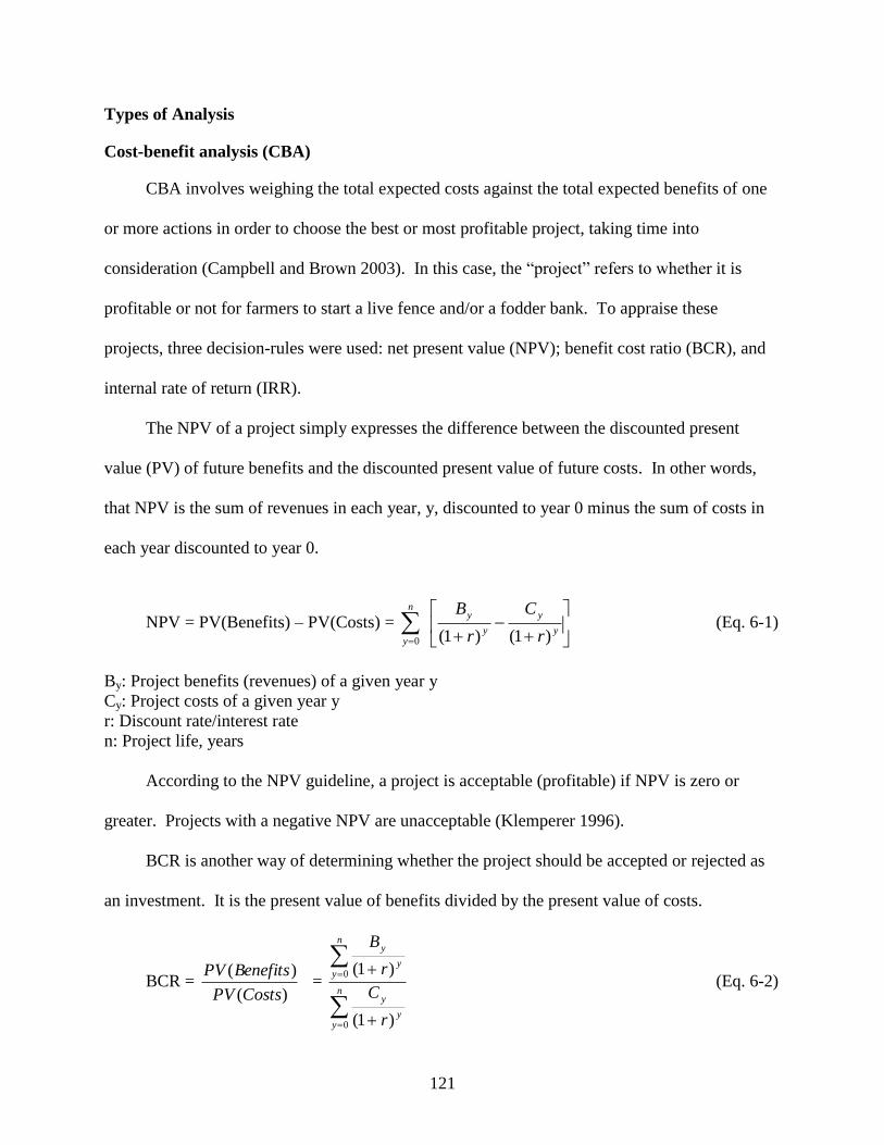
121
Types of Analysis
Cost-benefit analysis (CBA)
CBA involves weighing the total expected costs against the total expected benefits of one
or more actions in order to choose the best or most profitable project, taking time into
consideration (Campbell and Brown 2003). In this case, the ―project‖ refers to whether it is
profitable or not for farmers to start a live fence and/or a fodder bank. To appraise these
projects, three decision-rules were used: net present value (NPV); benefit cost ratio (BCR), and
internal rate of return (IRR).
The NPV of a project simply expresses the difference between the discounted present
value (PV) of future benefits and the discounted present value of future costs. In other words,
that NPV is the sum of revenues in each year, y, discounted to year 0 minus the sum of costs in
each year discounted to year 0.
NPV = PV(Benefits) – PV(Costs) =
y
y
y
yn
y r
C
r
B
)1()1(0
(Eq. 6-1)
By: Project benefits (revenues) of a given year y
Cy: Project costs of a given year y
r: Discount rate/interest rate
n: Project life, years
According to the NPV guideline, a project is acceptable (profitable) if NPV is zero or
greater. Projects with a negative NPV are unacceptable (Klemperer 1996).
BCR is another way of determining whether the project should be accepted or rejected as
an investment. It is the present value of benefits divided by the present value of costs.
BCR = )(
)(
CostsPV
BenefitsPV =
n
yy
y
n
yy
y
r
C
r
B
0
0
)1(
)1( (Eq. 6-2)
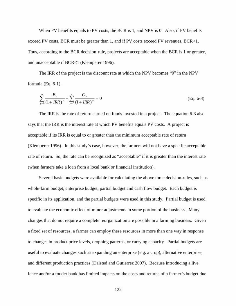
122
When PV benefits equals to PV costs, the BCR is 1, and NPV is 0. Also, if PV benefits
exceed PV costs, BCR must be greater than 1, and if PV costs exceed PV revenues, BCR<1.
Thus, according to the BCR decision-rule, projects are acceptable when the BCR is 1 or greater,
and unacceptable if BCR<1 (Klemperer 1996).
The IRR of the project is the discount rate at which the NPV becomes ―0‖ in the NPV
formula (Eq. 6-1).
0)1()1( 00
n
yy
yn
yy
y
IRR
C
IRR
B (Eq. 6-3)
The IRR is the rate of return earned on funds invested in a project. The equation 6-3 also
says that the IRR is the interest rate at which PV benefits equals PV costs. A project is
acceptable if its IRR is equal to or greater than the minimum acceptable rate of return
(Klemperer 1996). In this study‘s case, however, the farmers will not have a specific acceptable
rate of return. So, the rate can be recognized as ―acceptable‖ if it is greater than the interest rate
(when farmers take a loan from a local bank or financial institution).
Several basic budgets were available for calculating the above three decision-rules, such as
whole-farm budget, enterprise budget, partial budget and cash flow budget. Each budget is
specific in its application, and the partial budgets were used in this study. Partial budget is used
to evaluate the economic effect of minor adjustments in some portion of the business. Many
changes that do not require a complete reorganization are possible in a farming business. Given
a fixed set of resources, a farmer can employ these resources in more than one way in response
to changes in product price levels, cropping patterns, or carrying capacity. Partial budgets are
useful to evaluate changes such as expanding an enterprise (e.g. a crop), alternative enterprise,
and different production practices (Dalsted and Gutierrez 2007). Because introducing a live
fence and/or a fodder bank has limited impacts on the costs and returns of a farmer‘s budget due
123
to their small sizes, the partial budget was appropriate to use. Partial budgeting is based on the
principle that a small change in a farming business will have one or more of the following
effects: 1. Eliminate or reduce some costs, 2. Eliminate or reduce some benefits, 3. Cause
additional costs to be incurred, and 4. Cause additional returns to be received (Dalsted and
Gutierrez 2007). The net effects, i.e. NPV, BCR, and IRR, can be calculated from those four
components. Only the changes in costs and benefits that resulted directly from starting a live
fence and/or a fodder bank were collected/extracted from the survey data and taken to account in
the analysis.
The project cycle was set to 25 years. This is the expected rotation time for both live fence
and fodder bank tree species (personal communication with Dr. Bocary Kaya, 2006). The
growth curve was estimated based on the available data from biomass measurement. A discount
rate of 15 % was used, drawing on the information about standard interest rates applied by the
several local institutions for micro-credits (available to local farmers) in the study region (van
Dorp et al. 2005). Data collection and analysis were done with local currency, FCFA. It is
called CFA (Communaut Financiaire Africaine) franc, which is fixed against the euro at € 1 =
655.96 FCFA in 2006. When the results are shown in US dollar for the reference, exchange rate
of US$ 1 = 550 FCFA (average exchange rate during the field survey) was used.
Cost structure: Cost of seedlings was calculated following the method of Traoré et al.
(2003): an aggregation of the cost of seeds and the labor cost needed to grow seedlings in the
nursery. The average size of the fodder bank was 0.25 ha (50 m*50 m) the length of live-fence
rows was 200 m (50 m*4 with 800 trees) around to protect the fodder trees. Thus, planting and
maintaining these trees were included in the costs of fodder bank.
124
To protect the newly planted trees, dead fences (made from dead bush brunches) were
needed for the initial three years. Branches were obtained free of charge in the wild; no cash
costs were involved. To estimate the material cost of the dead fence, the volume of branches and
the price farmers would be willing to pay on the market were asked, and recalculated to the
standard size. The total average tool cost per farmer per year for the average size of live fence
was estimated 1,000 FCFA ($1.82) (van Dorp et al 2005). Since the fodder bank requires more
use of tools based on the data for required labor, the cost was set at 1,500 FCFA ($ 2.73) per
year.
To estimate the labor costs, farmers were asked for the average wage rate they pay for a
hired labor. The most common daily labor wage (7 hours work) was 750 FCFA ($ 1.36), ranging
between 500 and 1,000 FCFA ($ 0.91 – $ 1.82) depending on the season. The respondents of the
survey were also asked if they actually hired labor to install their fodder banks. The large
majority of them did not; instead they used their family members including children, or
exchanged the labor with neighbors.
Labor tasks are divided into:
1. Obtaining seedlings (or seeds)
2. Planting
3. Watering
4. Collecting materials for the dead fence
5. Constructing the dead fence around the live fence for protecting the seedlings (first three
years)
6. Maintenance of the live fence/fodder bank (weeding, replanting, pruning etc.)
7. Collecting products from the live fence and the fodder bank
8. Marketing live fence products (bringing to local market and selling)
9. Harvesting the timber/fuelwood at the end of the rotation
125
From the survey, the time farmers spent on each of the above tasks were estimated for
every year, and converted to the standard size and an average or median value was taken for the
CBA analysis. Median values were used when the sample population had extreme outliers. In
the cash flow chart, the labor time was calculated to monetary value, using the average labor
wage (Appendix B, C).
Benefit structure: Yields from live fence trees are:
Acacia nilotica: Fruits for tanning agent for the treatment of leather and traditional
medicines are sold in local markets. Branches are used as material for dead fences.
Acacia senegal: Bark is used as a traditional medicine, although it is not easily harvested,
and not sold in market.
Bauhinia rufescens: Leaves can be used as medicine, but not sold in the market.
Lawsonia inermis: Leaves are transformed into powder to be used for the dying of hands
and feet of women (cosmetic use), and highly valued in local markets.
Ziziphus mauritiana: Fruits are edible, but mostly for home consumption.
Benefits from these products were calculated in monetary value with local market price in
van Dorp study (2005). That data were used in this study‘s cash flow.
From the third year, farmers started harvesting the fodder (branches and leaves). Since the
fodder tree, Gliricidia sepium is an exotic species and had not been commonly used in the study
region, no market value was available for its fodder; none of the farmers interviewed had sold its
fodder in the market. Thus, the expected price of G. sepium fodder, if it is sold in the market,
was asked for in the survey, and the average of the answers was used to estimate the fodder
value. In addition, fodder bank provides another source of revenue, i.e. the saved time. The
owners were asked how many people and days they used to spend looking for fodder in the wild
before the fodder bank installation, as well as after they started harvesting from their fodder
banks. The difference is the saved time/labor, which they can use for other activities. The saved
126
time was then converted to monetary value using the labor wage, and counted as benefits of the
fodder bank in the cash flow.
Timber harvests at the end of rotation period (25 years) were also estimated by the
projected growth lines. The local market prices of timber and fuelwood were used to estimate
the monetary values. Eighty percent of trees planted in a live fence and a fodder bank is
assumed to produce a small log per tree, which can be sold in the local market at 700 – 1,500
FCFA ($ 1.27 – $ 2.73) per one cart (about 40 logs). The rest of trees and all branches, foliages
etc. (about 40% of the total expected biomass) were assumed to be sold as fuelwood which is
4,000-6,000 FCFA ($ 7.27 – $ 9.10) per one cart (250 – 300 kg) (personal communication with
ICRAF officers and local merchants, 2006).
C sale: Price of C varies quite largely at the international market. This study used the
average price for C emission trading in 2006, $42 per Mg C (World Bank 2006). Transaction
costs [which are the costs of arranging a contract (i.e. C sequestration project and consequent C
credit sale) and monitoring and enforcing the contract, as opposed to production costs
(implementation costs of the project)] were considered to be 0 in this cash flow. This is because
the transaction costs of agroforestry projects for C sequestration are usually covered by the third
party such as the project‘s trust fund (Scolel Té 2007). The trust fund deals with C buyers
(companies or individuals in developed countries) for the trade, monitors the project
performance, and provides the C payment and technical assistance to farmers.
The payment method of C credit is also a long debated issue in the negotiation of the
Kyoto Protocol and related meetings as discussed in Chapter 3. Two major payment methods
(Cacho et al. 2003b) were tried in this study for comparison.
127
Ideal accounting method: In this method, payments for C sequestration occur as the service
is provided and a debit occurs when C is released (i.e. by fire or harvest). Farmers annually
receive the payment according to the amount of C sequestered in their project‘s fields (live
fence/fodder bank). The full debit at harvest means that the total amount of C credits sale
received during the life of the project (live fence and/or fodder bank) are paid back to the
investor by farmers.
Tonne-year accounting method: Although the ideal accounting system is ―ideal‖ for the
land owners (i.e. farmers), it is risky for investors because they are not sure the project will last
until the end of the rotational age. The tonne-year method does not require redemption of C
credits upon harvest, because the payment occurs based only on the ‗equivalent‘ amount of
permanently avoided emissions during a given year (Moura-Costa and Wilson 2000). This
method has the advantage that no guarantee is needed if the project will last a required number of
years, as the annual payments are adjusted by the equivalent factor. This is a more favorable
method for the investors, and politically popular (Hardner et al 2000). In this study, the
equivalent factor of 0.0215 (Cacho et al. 2003a) was used. Farmers annually receive C credit
payment only equivalent to ―the amount of C sequestered in each year * 0.0215‖, but there is no
payment back to the investors at the end of the project.
These two methods were separately incorporated into the cash flow of both a live fence
project and a fodder bank project (see Appendix B, C). The decision rules (NPV, BCR, and
IRR) were calculated in three different cash flows: 1) Cash flow without C sale, 2) Cash flow
with C sale (ideal accounting), and 3) Cash flow with C sale (tonne-year accounting).
Sensitivity analysis
The calculation of NPV, BCR, or IRR in the CBA described above is based on the best
guess scenario where all variables of costs and benefits included in a cash flow are ―most likely‖
128
values such as an average of a data set. However, the future is uncertain: we do not know with
certainty what the future values of a project‘s costs and benefits will be. Sensitivity analysis is
the simple process of establishing the extent to which the outcome of the benefit-cost analysis is
sensitive to the assumed values of the inputs used in the analysis (Campbell and Brown 2003).
In this study, sensitivity of NPV to the change of major five input variable were tested and
presented in the results section. The tested variables were: 1) discount rate, 2) seedling cost, 3)
labor price (wage), 4) yield of harvests, and 5) C credit price. All variables except the discount
rate were changed +/- 50 % from the best guess scenario to compare which variable would affect
the NPV most. Discount rate was changed only +/- 5% because it was unreasonable to assume
the local discount rate to change largely (such as 50 %).
Risk modeling
Risk analysis refers to the identification and description of the nature of uncertainty
surrounding the project variables using probability distributions. When there is no appropriate
information on the expected range of values of input variable (= risks), only sensitivity analysis
can be done to observe the uncertainty of output projection. However, if some expectations are
available for the occurrence of the variability of the input variable, it is possible to conduct the
risk analysis. Each input variable has a range of possible values; high, medium, low; or,
maximum, mean, minimum. Risk modeling describes the likelihood of occurrence of these input
variables within the given range (probability distribution). The probability distribution for the
output (NPV) will then depend on the aggregation of probability distributions for these
individual input variables into a joint probability distribution.
The NPV probability distribution was simulated by a computer program called @RISK©
(Palisade Corporation). The program performs a simulation known as Monte Carlo analysis,
whereby the NPV of the projects is recalculated over and over again, each time using a different,
129
randomly chosen, set of values of input variables. The random selection of values is based on
the characteristics of each input variable‘s probability distribution. In this study, there was
insufficient information for the distribution of each four input variable (labor wage, seedling
cost, yield, and C credit price). Campbell and Brown (2003) recommended the use of a
triangular or ―three-point‖ distribution for this kind of analysis. This is the distribution described
by a high, low and best-guess estimate, which provide the maximum, minimum, and modal
values of the distribution respectively. Each input variable‘s distribution was set based on the
surveys data, observation, and personal communication with ICRAF field officers.
Labor wage distribution was likely to be between 500 and 1,000 FCFA (0.91-1.82 US$),
while 750 FCFA ($ 1.36)/man/day was the most prevalent labor wage. Seedling cost distribution
was assumed to be –50 % to +50 % from the best guess scenario. Harvests or yield distribution
was assumed to be 0 % to +50 % from the best guess scenario. C price was assumed to have a
range of $ 3.7 to $ 99 per Mg C, which was the minimum and maximum price traded in
international C market in 2006 (World Bank 2006). Mean price was $ 42/Mg C as used in the
best guess scenario.
Results
Demographic Characteristics of Target Population
Demographic characteristics (Table 6-1) were not based on data collected in the social
survey conducted in this study. However, the information on live fence farmers was already
available in the previous studies of ICRAF (Levasseur 2003; van Dorp et al. 2005). The fodder
bank owners who were interviewed in this study were mostly in the same village or neighboring
villages with similar conditions, and therefore their demographic characteristics were considered
to be similar. Average household size is 27.7 persons, consisting of 6.8 male members, 6.7
female members and 14.2 children. An active household member is a person actively
130
contributing to agricultural activities (male 4.9, female 5.2, children 5.7 on average). Non-active
members are generally sick or elderly, or children under 10 years old (9.2 on average). Also,
about 10 % of the household members have migrated from the village, usually for temporary
labor in the town of Ségou or other urban areas, to work or study. The average area of cultivated
land owned by a household is 15.3 ha. The main enterprise is millet, occupying more than 50 %
of total cultivating area. Other major crops include sorghum (2.3 ha), rice (2.1 ha) and
groundnut (0.9 ha). On average, each household possesses 3.6 work oxen (for agricultural labor
such as tillage), 5.8 cows (for breeding purposes), 2.1 donkeys, and other small livestock
including sheep, goats, and poultry.
Cost-Benefit Analysis: Best Guess Scenario of the Live Fence and the Fodder Bank
Based on the collected data, all costs and revenues (benefits) consisting of cash flow (year
0 to 25) were put into the spreadsheet. The cash flows of the live fence project and the fodder
bank project in the best guess scenario are shown in Appendix B, C. The net benefit, (total
revenues – total costs) of each year, was negative at the beginning, and turned positive from the
second year for both projects. Among components of costs, labor cost was the largest. Total
labor cost throughout the project year converted to present value was 60,738 FCFA ($ 110.4) for
the 291 m live fence project and 94,589 FCFA ($ 172.0) for the 0.25 ha fodder bank project.
Labor cost was high in the first three years for the live fence project compared with the rest of
the project term, because of the initial management such as construction of dead fence for
protecting seedlings. The fodder bank project needed more consistent management practices
(labor) than for the live fence project due to the fodder-tree management such as weeding and
pruning. Seedling cost was a relatively large component of the costs on net cash flow of both
projects, since it was initial investment (at year 0) and was not discounted to calculate the present
value.
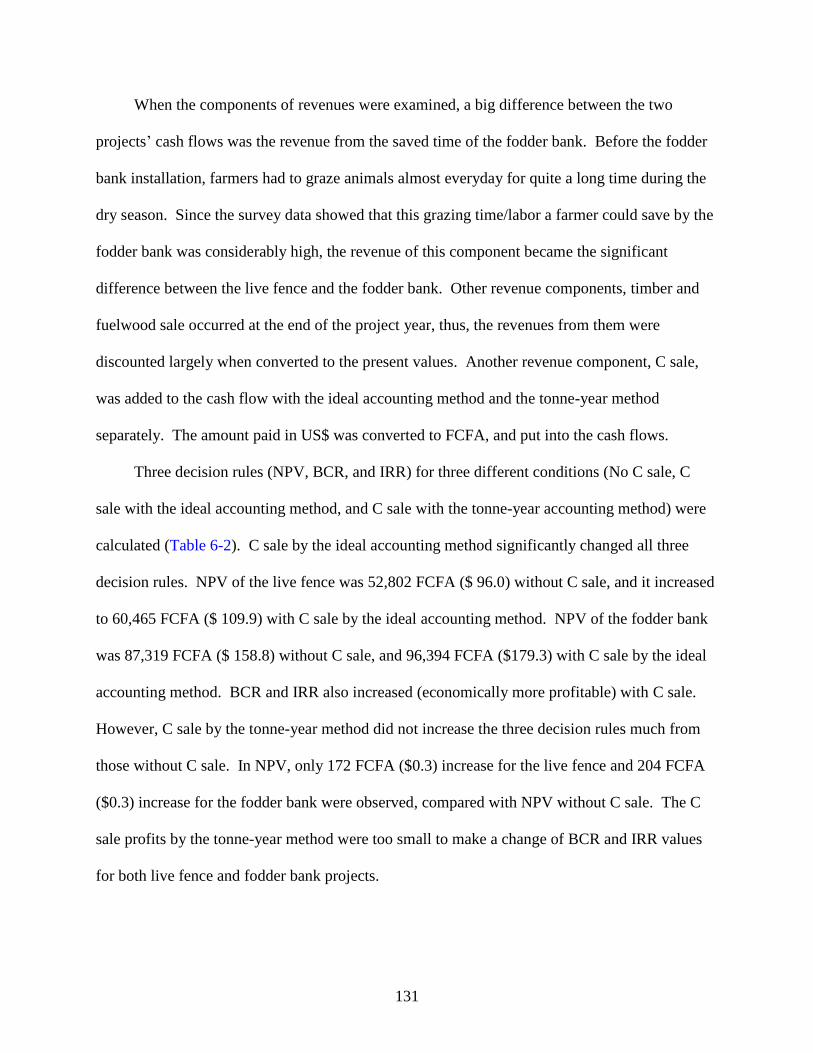
131
When the components of revenues were examined, a big difference between the two
projects‘ cash flows was the revenue from the saved time of the fodder bank. Before the fodder
bank installation, farmers had to graze animals almost everyday for quite a long time during the
dry season. Since the survey data showed that this grazing time/labor a farmer could save by the
fodder bank was considerably high, the revenue of this component became the significant
difference between the live fence and the fodder bank. Other revenue components, timber and
fuelwood sale occurred at the end of the project year, thus, the revenues from them were
discounted largely when converted to the present values. Another revenue component, C sale,
was added to the cash flow with the ideal accounting method and the tonne-year method
separately. The amount paid in US$ was converted to FCFA, and put into the cash flows.
Three decision rules (NPV, BCR, and IRR) for three different conditions (No C sale, C
sale with the ideal accounting method, and C sale with the tonne-year accounting method) were
calculated (Table 6-2). C sale by the ideal accounting method significantly changed all three
decision rules. NPV of the live fence was 52,802 FCFA ($ 96.0) without C sale, and it increased
to 60,465 FCFA ($ 109.9) with C sale by the ideal accounting method. NPV of the fodder bank
was 87,319 FCFA ($ 158.8) without C sale, and 96,394 FCFA ($179.3) with C sale by the ideal
accounting method. BCR and IRR also increased (economically more profitable) with C sale.
However, C sale by the tonne-year method did not increase the three decision rules much from
those without C sale. In NPV, only 172 FCFA ($0.3) increase for the live fence and 204 FCFA
($0.3) increase for the fodder bank were observed, compared with NPV without C sale. The C
sale profits by the tonne-year method were too small to make a change of BCR and IRR values
for both live fence and fodder bank projects.
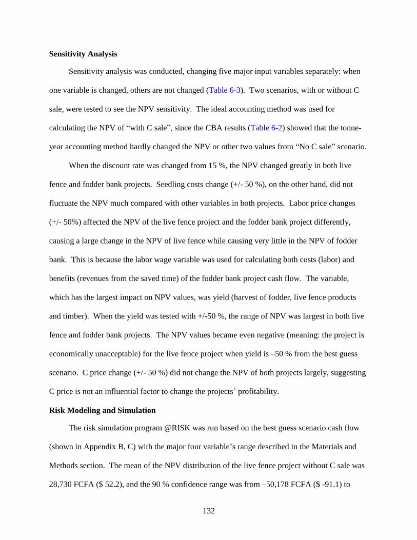
132
Sensitivity Analysis
Sensitivity analysis was conducted, changing five major input variables separately: when
one variable is changed, others are not changed (Table 6-3). Two scenarios, with or without C
sale, were tested to see the NPV sensitivity. The ideal accounting method was used for
calculating the NPV of ―with C sale‖, since the CBA results (Table 6-2) showed that the tonne-
year accounting method hardly changed the NPV or other two values from ―No C sale‖ scenario.
When the discount rate was changed from 15 %, the NPV changed greatly in both live
fence and fodder bank projects. Seedling costs change (+/- 50 %), on the other hand, did not
fluctuate the NPV much compared with other variables in both projects. Labor price changes
(+/- 50%) affected the NPV of the live fence project and the fodder bank project differently,
causing a large change in the NPV of live fence while causing very little in the NPV of fodder
bank. This is because the labor wage variable was used for calculating both costs (labor) and
benefits (revenues from the saved time) of the fodder bank project cash flow. The variable,
which has the largest impact on NPV values, was yield (harvest of fodder, live fence products
and timber). When the yield was tested with +/-50 %, the range of NPV was largest in both live
fence and fodder bank projects. The NPV values became even negative (meaning: the project is
economically unacceptable) for the live fence project when yield is –50 % from the best guess
scenario. C price change (+/- 50 %) did not change the NPV of both projects largely, suggesting
C price is not an influential factor to change the projects‘ profitability.
Risk Modeling and Simulation
The risk simulation program @RISK was run based on the best guess scenario cash flow
(shown in Appendix B, C) with the major four variable‘s range described in the Materials and
Methods section. The mean of the NPV distribution of the live fence project without C sale was
28,730 FCFA ($ 52.2), and the 90 % confidence range was from –50,178 FCFA ($ -91.1) to
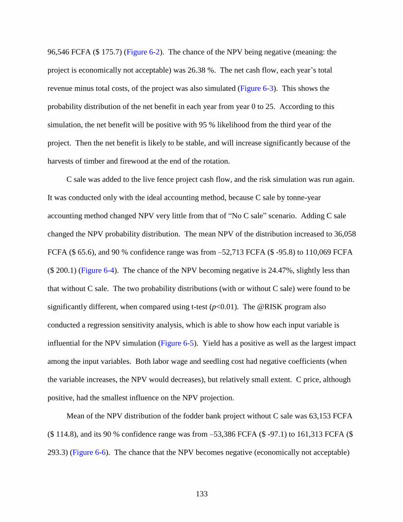
133
96,546 FCFA ($ 175.7) (Figure 6-2). The chance of the NPV being negative (meaning: the
project is economically not acceptable) was 26.38 %. The net cash flow, each year‘s total
revenue minus total costs, of the project was also simulated (Figure 6-3). This shows the
probability distribution of the net benefit in each year from year 0 to 25. According to this
simulation, the net benefit will be positive with 95 % likelihood from the third year of the
project. Then the net benefit is likely to be stable, and will increase significantly because of the
harvests of timber and firewood at the end of the rotation.
C sale was added to the live fence project cash flow, and the risk simulation was run again.
It was conducted only with the ideal accounting method, because C sale by tonne-year
accounting method changed NPV very little from that of ―No C sale‖ scenario. Adding C sale
changed the NPV probability distribution. The mean NPV of the distribution increased to 36,058
FCFA ($ 65.6), and 90 % confidence range was from –52,713 FCFA ($ -95.8) to 110,069 FCFA
($ 200.1) (Figure 6-4). The chance of the NPV becoming negative is 24.47%, slightly less than
that without C sale. The two probability distributions (with or without C sale) were found to be
significantly different, when compared using t-test (p<0.01). The @RISK program also
conducted a regression sensitivity analysis, which is able to show how each input variable is
influential for the NPV simulation (Figure 6-5). Yield has a positive as well as the largest impact
among the input variables. Both labor wage and seedling cost had negative coefficients (when
the variable increases, the NPV would decreases), but relatively small extent. C price, although
positive, had the smallest influence on the NPV projection.
Mean of the NPV distribution of the fodder bank project without C sale was 63,153 FCFA
($ 114.8), and its 90 % confidence range was from –53,386 FCFA ($ -97.1) to 161,313 FCFA ($
293.3) (Figure 6-6). The chance that the NPV becomes negative (economically not acceptable)
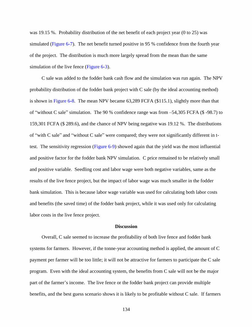
134
was 19.15 %. Probability distribution of the net benefit of each project year (0 to 25) was
simulated (Figure 6-7). The net benefit turned positive in 95 % confidence from the fourth year
of the project. The distribution is much more largely spread from the mean than the same
simulation of the live fence (Figure 6-3).
C sale was added to the fodder bank cash flow and the simulation was run again. The NPV
probability distribution of the fodder bank project with C sale (by the ideal accounting method)
is shown in Figure 6-8. The mean NPV became 63,289 FCFA ($115.1), slightly more than that
of ―without C sale‖ simulation. The 90 % confidence range was from –54,305 FCFA ($ -98.7) to
159,301 FCFA ($ 289.6), and the chance of NPV being negative was 19.12 %. The distributions
of ―with C sale‖ and ―without C sale‖ were compared; they were not significantly different in t-
test. The sensitivity regression (Figure 6-9) showed again that the yield was the most influential
and positive factor for the fodder bank NPV simulation. C price remained to be relatively small
and positive variable. Seedling cost and labor wage were both negative variables, same as the
results of the live fence project, but the impact of labor wage was much smaller in the fodder
bank simulation. This is because labor wage variable was used for calculating both labor costs
and benefits (the saved time) of the fodder bank project, while it was used only for calculating
labor costs in the live fence project.
Discussion
Overall, C sale seemed to increase the profitability of both live fence and fodder bank
systems for farmers. However, if the tonne-year accounting method is applied, the amount of C
payment per farmer will be too little; it will not be attractive for farmers to participate the C sale
program. Even with the ideal accounting system, the benefits from C sale will not be the major
part of the farmer‘s income. The live fence or the fodder bank project can provide multiple
benefits, and the best guess scenario shows it is likely to be profitable without C sale. If farmers
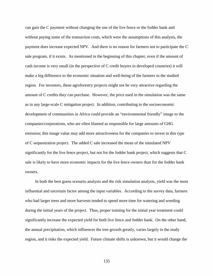
135
can gain the C payment without changing the use of the live fence or the fodder bank and
without paying some of the transaction costs, which were the assumptions of this analysis, the
payment does increase expected NPV. And there is no reason for farmers not to participate the C
sale program, if it exists. As mentioned in the beginning of this chapter, even if the amount of
cash income is very small (in the perspective of C credit buyers in developed countries) it will
make a big difference to the economic situation and well-being of the farmers in the studied
region. For investors, these agroforestry projects might not be very attractive regarding the
amount of C credits they can purchase. However, the price used in the simulation was the same
as in any large-scale C mitigation project. In addition, contributing to the socioeconomic
development of communities in Africa could provide an ―environmental friendly‖ image to the
companies/corporations, who are often blamed as responsible for large amounts of GHG
emission; this image value may add more attractiveness for the companies to invest in this type
of C sequestration project. The added C sale increased the mean of the simulated NPV
significantly for the live fence project, but not for the fodder bank project, which suggests that C
sale is likely to have more economic impacts for the live fence owners than for the fodder bank
owners.
In both the best guess scenario analysis and the risk simulation analysis, yield was the most
influential and uncertain factor among the input variables. According to the survey data, farmers
who had larger trees and more harvests tended to spend more time for watering and weeding
during the initial years of the project. Thus, proper training for the initial year treatment could
significantly increase the expected yield for both live fence and fodder bank. On the other hand,
the annual precipitation, which influences the tree growth greatly, varies largely in the study
region, and it risks the expected yield. Future climate shifts is unknown, but it would change the
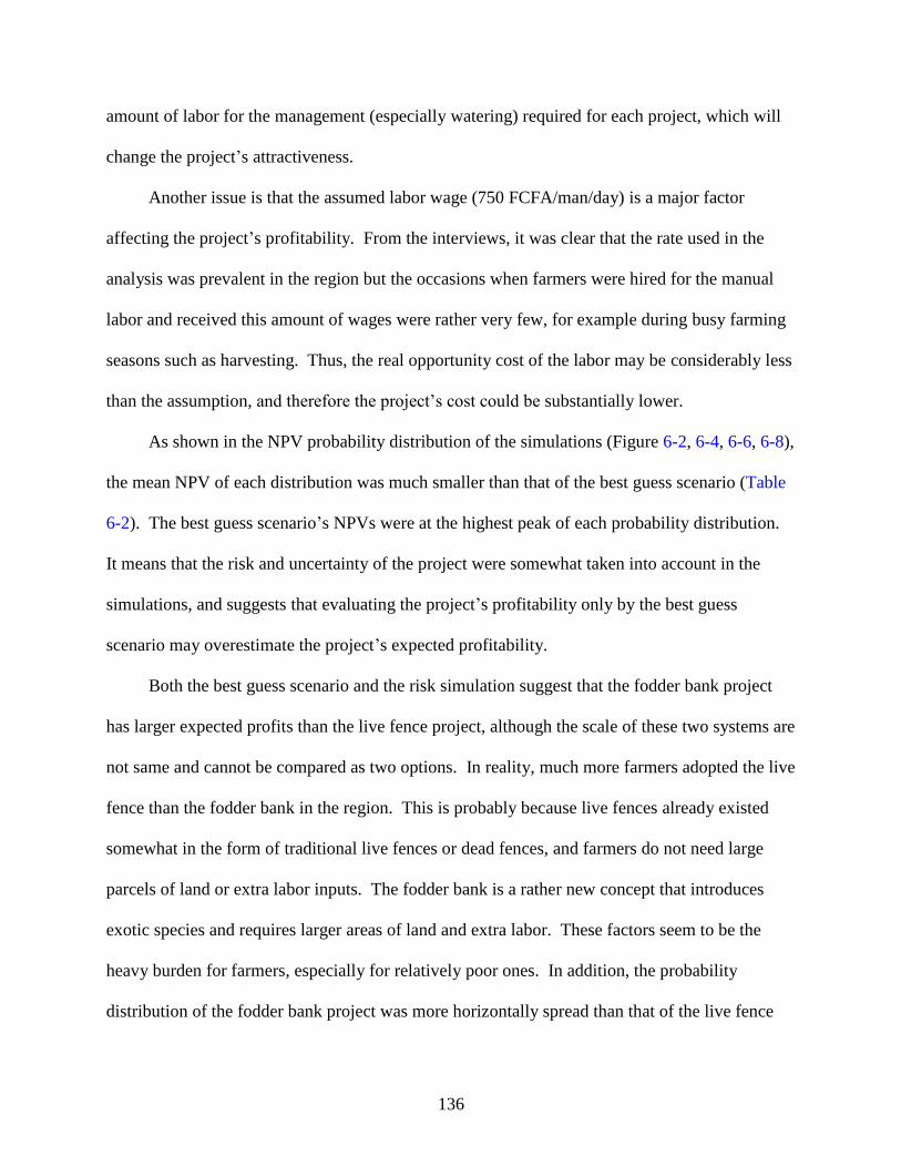
136
amount of labor for the management (especially watering) required for each project, which will
change the project‘s attractiveness.
Another issue is that the assumed labor wage (750 FCFA/man/day) is a major factor
affecting the project‘s profitability. From the interviews, it was clear that the rate used in the
analysis was prevalent in the region but the occasions when farmers were hired for the manual
labor and received this amount of wages were rather very few, for example during busy farming
seasons such as harvesting. Thus, the real opportunity cost of the labor may be considerably less
than the assumption, and therefore the project‘s cost could be substantially lower.
As shown in the NPV probability distribution of the simulations (Figure 6-2, 6-4, 6-6, 6-8),
the mean NPV of each distribution was much smaller than that of the best guess scenario (Table
6-2). The best guess scenario‘s NPVs were at the highest peak of each probability distribution.
It means that the risk and uncertainty of the project were somewhat taken into account in the
simulations, and suggests that evaluating the project‘s profitability only by the best guess
scenario may overestimate the project‘s expected profitability.
Both the best guess scenario and the risk simulation suggest that the fodder bank project
has larger expected profits than the live fence project, although the scale of these two systems are
not same and cannot be compared as two options. In reality, much more farmers adopted the live
fence than the fodder bank in the region. This is probably because live fences already existed
somewhat in the form of traditional live fences or dead fences, and farmers do not need large
parcels of land or extra labor inputs. The fodder bank is a rather new concept that introduces
exotic species and requires larger areas of land and extra labor. These factors seem to be the
heavy burden for farmers, especially for relatively poor ones. In addition, the probability
distribution of the fodder bank project was more horizontally spread than that of the live fence
137
project (Figure 6-2, 6-6), and the net benefit flow of the fodder bank had wider probability range
than that of the live fence (Figure 6-3, 6-7). This suggests that the fodder bank has a higher
chance of NPV fluctuation. Overall, the fodder bank seems to be a high risk, high return project
than the live fence. The majority of the farmers in the region are subsistence oriented and are
expected to be very risk averse. Profitability may not be the first consideration in their adoption
process. Other factors, such as water or labor availability and the presence of fodder in the open
land nearby might be the more important factors in the adoption of the fodder bank, if they are to
be promoted.
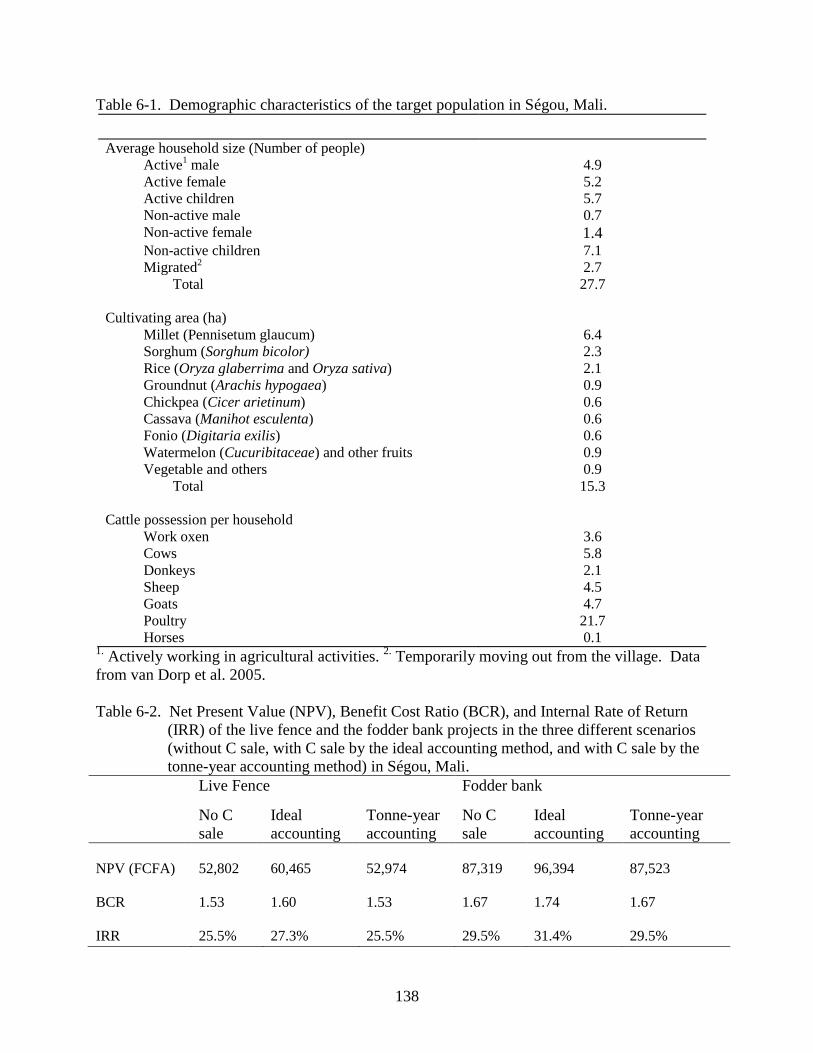
138
Table 6-1. Demographic characteristics of the target population in Ségou, Mali.
Average household size (Number of people)
Active1 male 4.9
Active female 5.2
Active children 5.7
Non-active male 0.7 Non-active female 1.4
Non-active children 7.1
Migrated2 2.7
Total 27.7
Cultivating area (ha)
Millet (Pennisetum glaucum) 6.4
Sorghum (Sorghum bicolor) 2.3
Rice (Oryza glaberrima and Oryza sativa) 2.1
Groundnut (Arachis hypogaea) 0.9
Chickpea (Cicer arietinum) 0.6
Cassava (Manihot esculenta) 0.6
Fonio (Digitaria exilis) 0.6
Watermelon (Cucuribitaceae) and other fruits 0.9
Vegetable and others 0.9
Total 15.3
Cattle possession per household
Work oxen 3.6
Cows 5.8
Donkeys 2.1
Sheep 4.5
Goats 4.7
Poultry 21.7
Horses 0.1 1.
Actively working in agricultural activities. 2.
Temporarily moving out from the village. Data
from van Dorp et al. 2005.
Table 6-2. Net Present Value (NPV), Benefit Cost Ratio (BCR), and Internal Rate of Return
(IRR) of the live fence and the fodder bank projects in the three different scenarios
(without C sale, with C sale by the ideal accounting method, and with C sale by the
tonne-year accounting method) in Ségou, Mali.
Live Fence Fodder bank
No C
sale
Ideal
accounting
Tonne-year
accounting
No C
sale
Ideal
accounting
Tonne-year
accounting
NPV (FCFA)
52,802
60,465
52,974
87,319
96,394
87,523
BCR
1.53
1.60
1.53
1.67
1.74
1.67
IRR
25.5%
27.3%
25.5%
29.5%
31.4%
29.5%
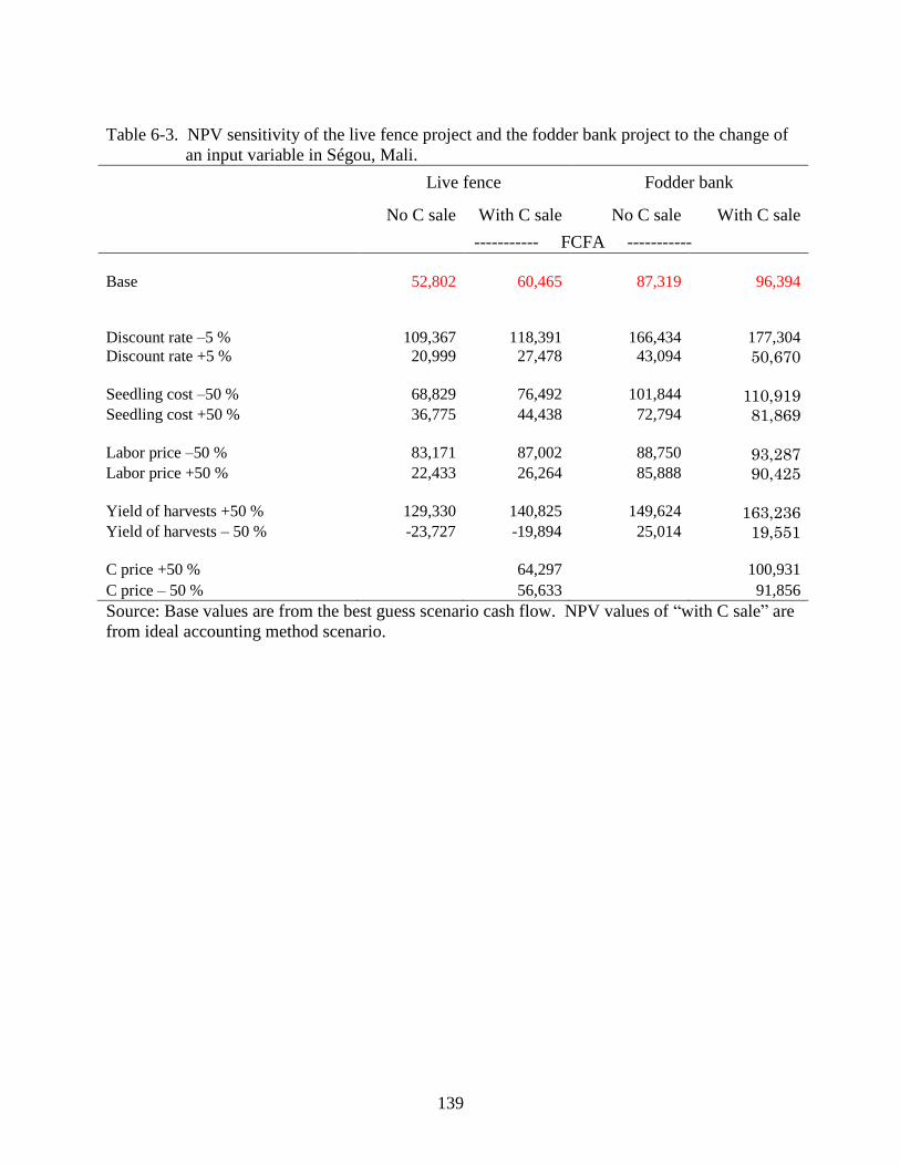
139
Table 6-3. NPV sensitivity of the live fence project and the fodder bank project to the change of
an input variable in Ségou, Mali.
Live fence Fodder bank
No C sale With C sale No C sale With C sale
----------- FCFA -----------
Base
52,802
60,465
87,319
96,394
Discount rate –5 %
109,367
118,391
166,434
177,304
Discount rate +5 % 20,999 27,478 43,094 50,670
Seedling cost –50 %
68,829
76,492
101,844
110,919 Seedling cost +50 % 36,775 44,438 72,794 81,869
Labor price –50 %
83,171
87,002
88,750
93,287 Labor price +50 % 22,433 26,264 85,888 90,425
Yield of harvests +50 %
129,330
140,825
149,624
163,236 Yield of harvests – 50 % -23,727 -19,894 25,014 19,551
C price +50 %
64,297
100,931
C price – 50 % 56,633 91,856
Source: Base values are from the best guess scenario cash flow. NPV values of ―with C sale‖ are
from ideal accounting method scenario.
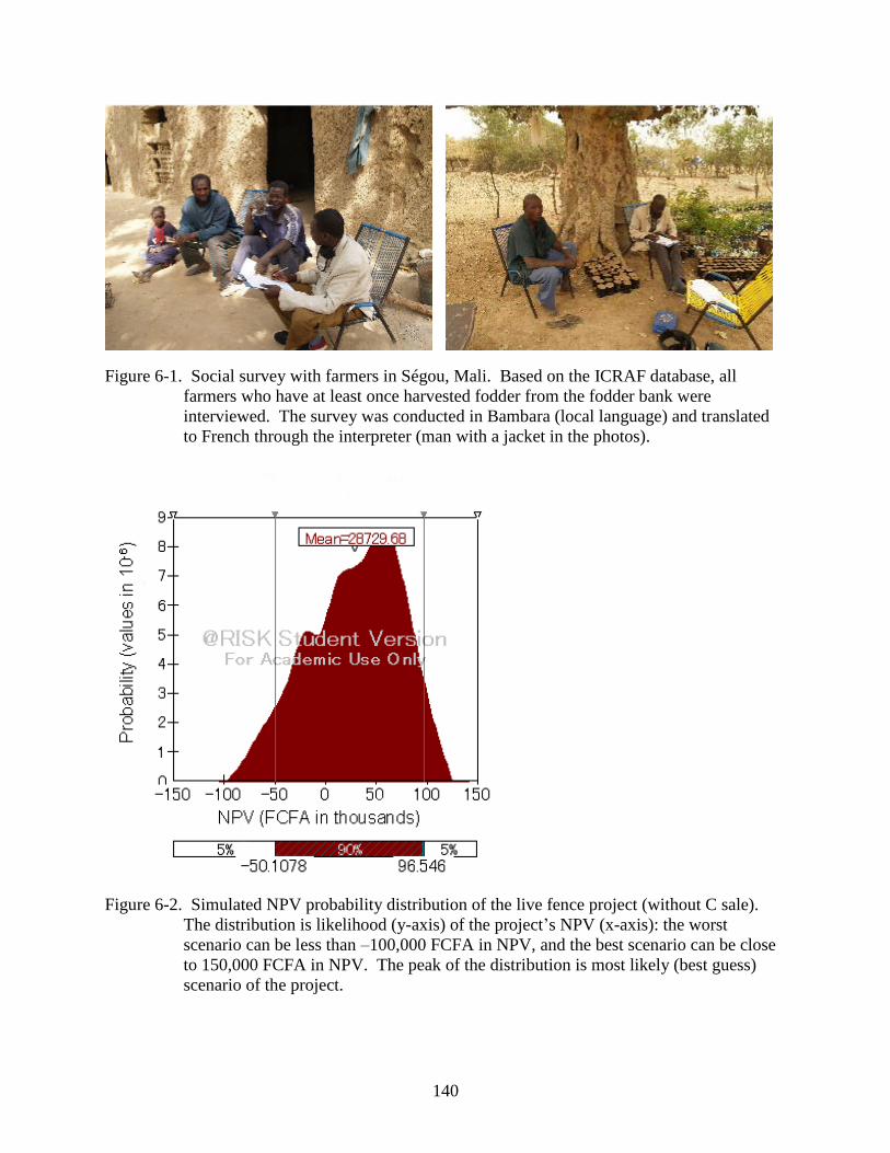
140
Figure 6-1. Social survey with farmers in Ségou, Mali. Based on the ICRAF database, all
farmers who have at least once harvested fodder from the fodder bank were
interviewed. The survey was conducted in Bambara (local language) and translated
to French through the interpreter (man with a jacket in the photos).
Figure 6-2. Simulated NPV probability distribution of the live fence project (without C sale).
The distribution is likelihood (y-axis) of the project‘s NPV (x-axis): the worst
scenario can be less than –100,000 FCFA in NPV, and the best scenario can be close
to 150,000 FCFA in NPV. The peak of the distribution is most likely (best guess)
scenario of the project.
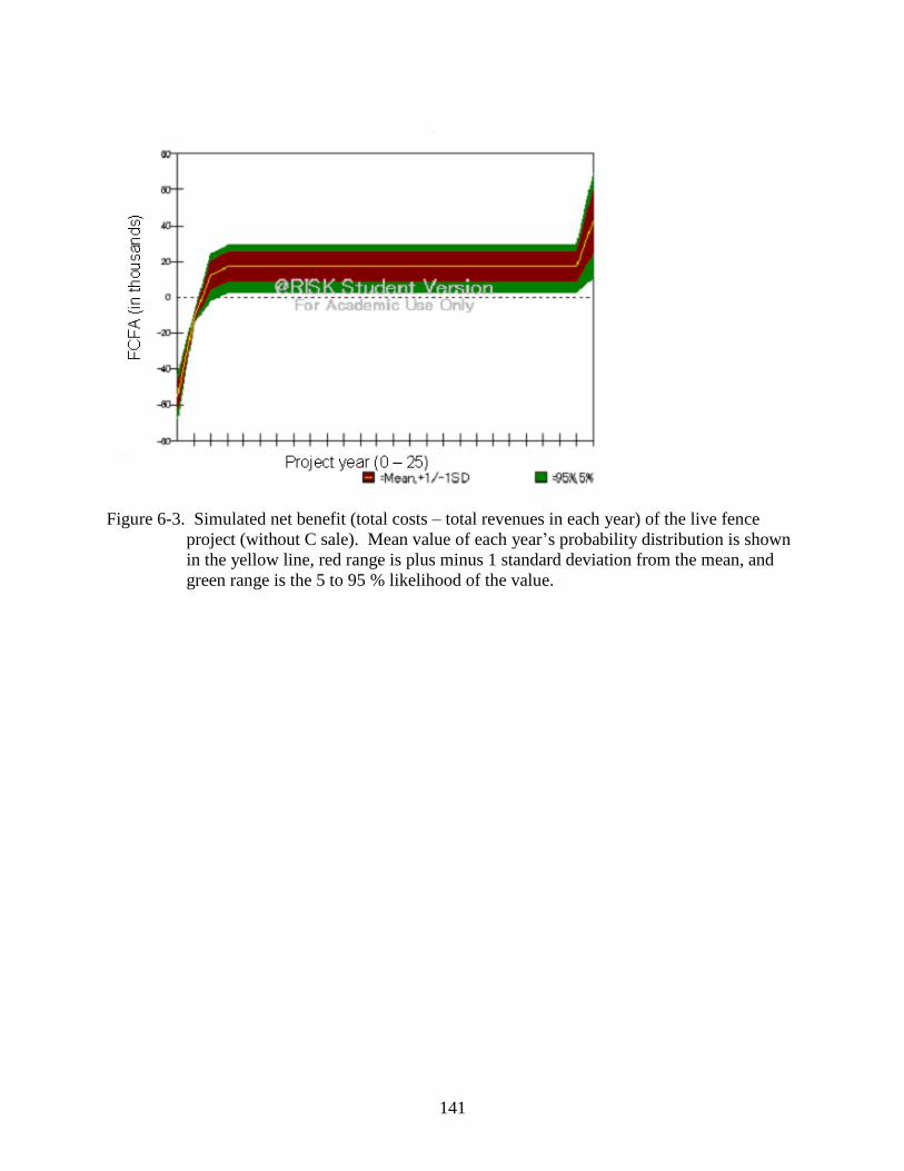
141
Figure 6-3. Simulated net benefit (total costs – total revenues in each year) of the live fence
project (without C sale). Mean value of each year‘s probability distribution is shown
in the yellow line, red range is plus minus 1 standard deviation from the mean, and
green range is the 5 to 95 % likelihood of the value.
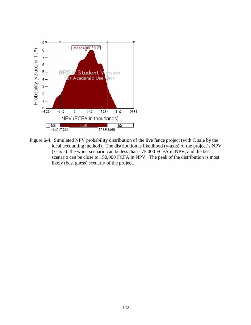
142
Figure 6-4. Simulated NPV probability distribution of the live fence project (with C sale by the
ideal accounting method). The distribution is likelihood (y-axis) of the project‘s NPV
(x-axis): the worst scenario can be less than –75,000 FCFA in NPV, and the best
scenario can be close to 150,000 FCFA in NPV. The peak of the distribution is most
likely (best guess) scenario of the project.
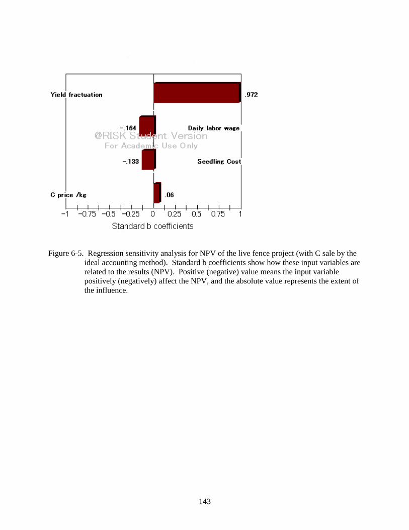
143
Figure 6-5. Regression sensitivity analysis for NPV of the live fence project (with C sale by the
ideal accounting method). Standard b coefficients show how these input variables are
related to the results (NPV). Positive (negative) value means the input variable
positively (negatively) affect the NPV, and the absolute value represents the extent of
the influence.
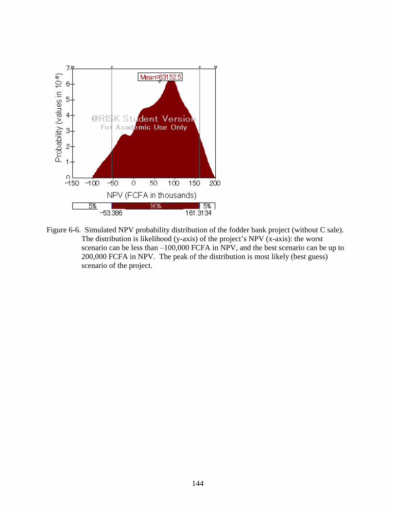
144
Figure 6-6. Simulated NPV probability distribution of the fodder bank project (without C sale).
The distribution is likelihood (y-axis) of the project‘s NPV (x-axis): the worst
scenario can be less than –100,000 FCFA in NPV, and the best scenario can be up to
200,000 FCFA in NPV. The peak of the distribution is most likely (best guess)
scenario of the project.

145
Figure 6-7. Simulated net benefit (total costs – total revenues in each year) of the fodder bank
project (without C sale). Mean value of each year‘s probability distribution is shown
in the yellow line, red range is plus minus 1 standard deviation from the mean, and
green range is the 5 to 95 % likelihood of the value.
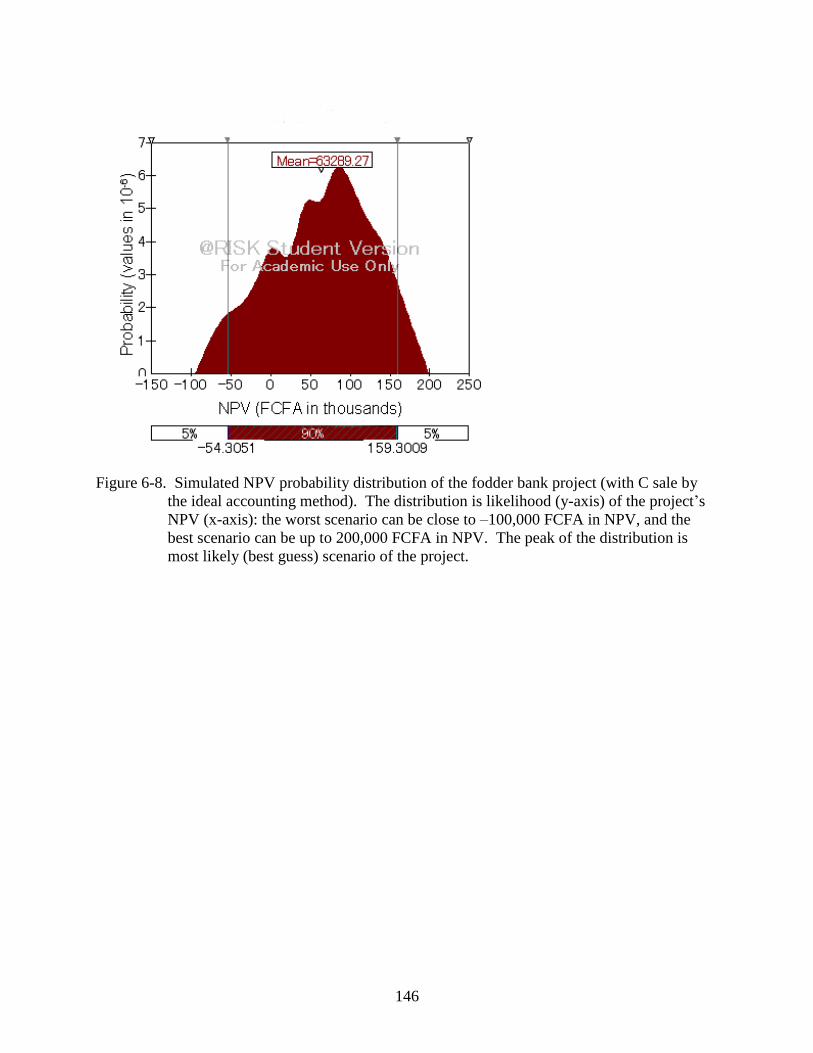
146
Figure 6-8. Simulated NPV probability distribution of the fodder bank project (with C sale by
the ideal accounting method). The distribution is likelihood (y-axis) of the project‘s
NPV (x-axis): the worst scenario can be close to –100,000 FCFA in NPV, and the
best scenario can be up to 200,000 FCFA in NPV. The peak of the distribution is
most likely (best guess) scenario of the project.
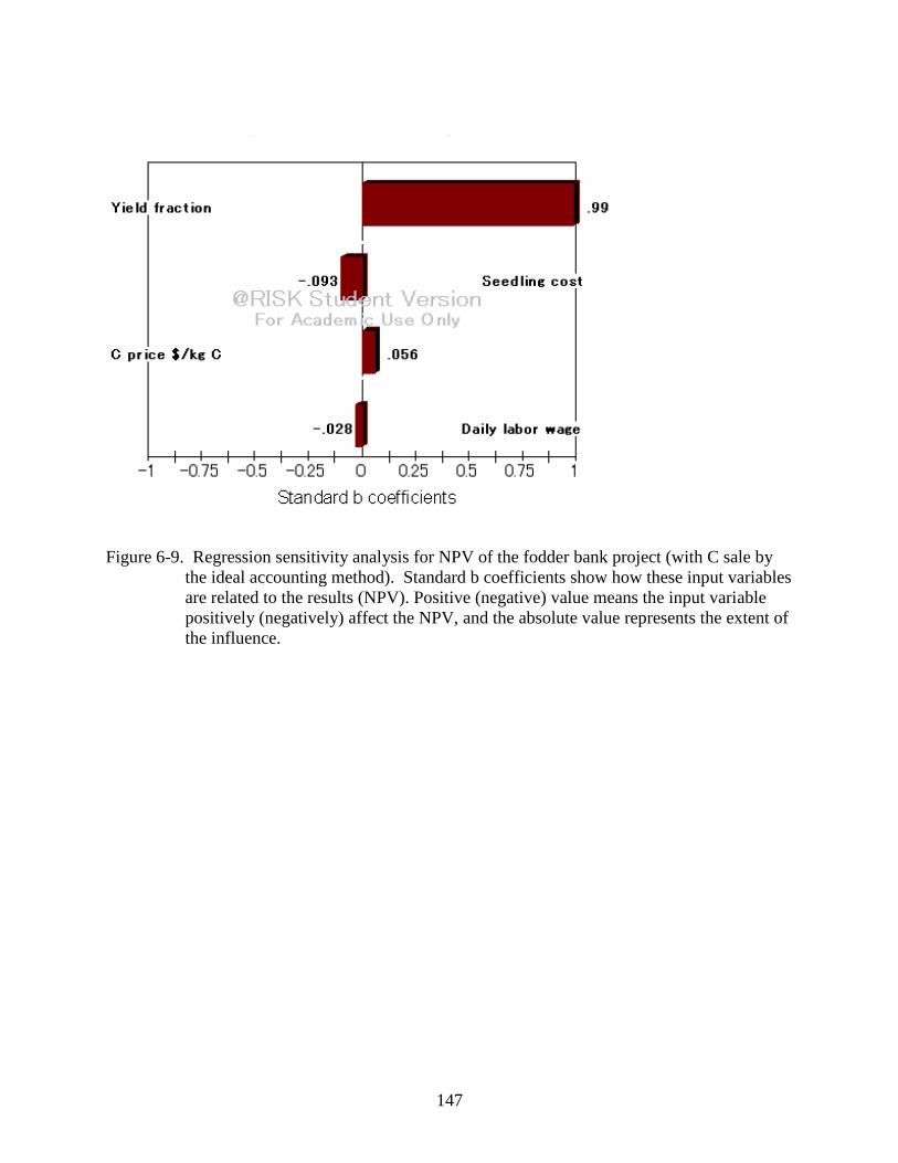
147
Figure 6-9. Regression sensitivity analysis for NPV of the fodder bank project (with C sale by
the ideal accounting method). Standard b coefficients show how these input variables
are related to the results (NPV). Positive (negative) value means the input variable
positively (negatively) affect the NPV, and the absolute value represents the extent of
the influence.
148
CHAPTER 7
SUMMARY AND CONCLUSIONS
This dissertation study examined the carbon (C) sequestration potential of major
agroforestry practices in Ségou Region, Mali, of the West African Sahel (WAS), and analyzed
the feasibility and socioeconomic characteristics of the selected agroforestry systems in the
context of C sequestration services. The selected systems were two traditional parkland
agroforestry systems with Faidherbia albida or Vitellaria paradoxa as the dominant tree species,
two newly introduced (improved) agroforestry systems (live fence and fodder bank), and a so-
called ―abandoned‖ (degraded) land. The research revolved around four major questions.
1. How much C is stored in different agroforestry systems aboveground and belowground?
2. Do trees contribute to store C in soil, and how stable is that C?
3. What is the overall relative attractiveness of each of the selected agroforestry systems in
terms of its C sequestration potential?
4. If C credit markets were available, would adopting agroforestry provide more profits to
land owners?
C Sequestration Potential
Biophysical Potential
The selected agroforestry systems proved to have potentials for sequestering more C both
above- and belowground than the tree-less cultivated land in the study region. However, the
estimated amounts of C stored in these systems and sequestered after the systems‘ establishment
are quite variable depending on the baseline (without project) status as well as the accounting
method used.
The two traditional parklands store significant amounts of C in the biomass C. Especially,
the large F. albida trees (average DBH 59.4 cm, height 13 m) store considerable amounts of C.
However, parklands are not likely to be considered for C sequestration projects anytime soon,
149
because Kyoto Protocol currently admits only C sequestered as a result of newly implemented
mitigation projects, and traditional land-use systems such as parklands and forest conservation –
sustaining parklands – are not recognized as emission-reduction activities under the Protocol at
least until 2012.
On the other hand, improved agroforestry systems (live fence and fodder bank) were found
to have a better chance to be recognized as C sequestering activities than parkland systems.
Because these systems are newly introduced, most of the biomass stored in the systems can be
counted as ―sequestered‖ C credits, although their potentials as C sequestration projects were not
as high as expected. C sequestration potential of a land-use system has to be expressed on a unit-
area basis for a given period of time. From that perspective, some improved agroforestry
systems (live fence and fodder bank, in this study) do not rank high because of the nature of their
planting configurations and/or management requirements. Live fence trees are densely planted
along rows such that the individual trees are not ―allowed‖ to grow fully; moreover, the fence
rows are on plot boundaries and therefore the area occupied or influenced by a fence row in
relation to the total area of the plot it borders is low. As far as the fodder banks are concerned,
the fodder trees that are frequently harvested for their leafy biomass cannot obviously be
expected to store large quantities of biomass C. Therefore, the absolute amounts of C stored in
these systems per unit area would not be as large as that for, say, parklands. While the amounts
of biomass C stored (calculated from general allometric equations following UNFCCC
guidelines) were 54.0 and 22.4 Mg C ha-1
respectively for 40-year or older stands of F. albida
and V. paradoxa parkland systems, the amounts were 4.7 Mg C ha-1
for a 8-year-old stand of live
fence and 2.2 Mg C ha-1
for 6 – 9 –year-old stand of fodder bank.
150
Another issue is that the initial C loss (both in biomass and soil) resulting from land
clearing and tillage for facilitating tree establishment in these improved practices is expected to
be significant; this loss may not be compensated by the planted trees any time soon, given their
slow growth rates owing to poor soil fertility and adverse climatic conditions. Therefore,
introducing these improved systems in abandoned land for land amelioration, as the World
Agroforestry Centre (ICRAF) is promoting, may not make a significant contribution to net C
sequestration in the near term; indeed it is likely to cause net negative C balance in the initial
stage of implementation.
Currently soil C is not considered to be tradable, but the relative portion of soil C in the
studied systems turned out to be comparatively large. For example, the percentages of soil C (0
– 100 cm) in total C (biomass C + soil C 0 – 100 cm) stock of the studied agroforestry systems
were 38 % in F. albida parkland, 55 % in V. paradoxa parkland, 84 % in live fence, and 94 % in
fodder bank. This cannot be ignored when the potential for long-term storage is considered.
Soil fractionation studies and isotopic ratio measurements showed that tree litter tends to
increase unprotected, relatively new C on the surface soil. In the deeper soil, the parklands that
have had trees in the system for a long time were likely to hold more protected C than the newly
introduced live fence or fodder bank systems. Also, management practices such as tillage and
litter usage seemed to have a large influence on soil C accumulation.
Socioecomic Potential
The cost-benefit analysis suggested that live fence and fodder bank were likely to be
profitable for farmers, whether with or without C sale. C sale changed the profitability: $ 13.9
more in net present value (NPV) of average-size live fence (291 m), and $ 20.5 more in NPV of
average size fodder bank (0.25 ha). These estimations are based on the assumptions of 25-year
rotation, no transaction costs on the farmers, and an accounting method ideal to C sellers
151
(farmers); all of these assumptions are subject to change. With the accounting method that is in
favor for the investors, the expected profits from C sale in the same model produced an increase
in NPV of only about $ 0.3 in both systems. Even in the local currency with farmer‘s monetary
values, $ 0.3 increase in NPV is almost nothing for a 25-year project. Thus, it is clear that the
accounting method is a very strong factor to determine whether C sale through agroforestry
should be introduced to the region.
Also, sensitivity analysis and risk analysis showed that C price did not have a major
influence on changing the cost and benefit flow of both systems. It would contribute to the
increase of profitability but had relatively small effect compared with other major variables such
as yield, labor cost, and seedling cost. On the other hand, tree growth (yield) had a strong
influence on the project‘s profitability. Regression sensitivity analysis showed that the effect of
yield was 10 times or more strong than that of other factors. Since natural environment such as
rainfall and pests greatly affects tree growth, the uncertainty (risk) regarding yield (whether tree
would grow expectedly or not) is quite difficult to control and is a major discouraging factor for
applying the improved agroforestry in general, whether with or without C sale.
Regarding relative attractiveness of live fence and fodder bank, it was difficult to compare
because the scale of the project (the land needed) was different in the simulation of two systems.
The fodder bank project that needs about three times more land (and correspondingly higher
labor cost) than live fence project showed larger range of expected NPV ($ -98.7 to $ 289.6 in
fodder bank vs. $ -95.8 to $ 65.6 in live fence). Considering that improved agroforestry systems
require ―additional‖ work for farmer‘s cultivation practices and that their resources (land, money
for buying seeds, etc.) are very limited, live fence would be easier and less risky project for them
to implement.
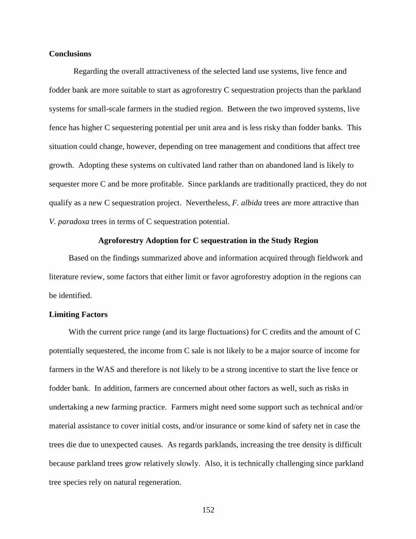
152
Conclusions
Regarding the overall attractiveness of the selected land use systems, live fence and
fodder bank are more suitable to start as agroforestry C sequestration projects than the parkland
systems for small-scale farmers in the studied region. Between the two improved systems, live
fence has higher C sequestering potential per unit area and is less risky than fodder banks. This
situation could change, however, depending on tree management and conditions that affect tree
growth. Adopting these systems on cultivated land rather than on abandoned land is likely to
sequester more C and be more profitable. Since parklands are traditionally practiced, they do not
qualify as a new C sequestration project. Nevertheless, F. albida trees are more attractive than
V. paradoxa trees in terms of C sequestration potential.
Agroforestry Adoption for C sequestration in the Study Region
Based on the findings summarized above and information acquired through fieldwork and
literature review, some factors that either limit or favor agroforestry adoption in the regions can
be identified.
Limiting Factors
With the current price range (and its large fluctuations) for C credits and the amount of C
potentially sequestered, the income from C sale is not likely to be a major source of income for
farmers in the WAS and therefore is not likely to be a strong incentive to start the live fence or
fodder bank. In addition, farmers are concerned about other factors as well, such as risks in
undertaking a new farming practice. Farmers might need some support such as technical and/or
material assistance to cover initial costs, and/or insurance or some kind of safety net in case the
trees die due to unexpected causes. As regards parklands, increasing the tree density is difficult
because parkland trees grow relatively slowly. Also, it is technically challenging since parkland
tree species rely on natural regeneration.

153
Soil C estimation is far more labor-intensive and costly than biomass C estimation, and
methods of measurements/accounting are still under discussion. Even in the same land use
system, the amount of soil C per unit area can vary depending on the depth of sampling and/or
the instruments used to measure C content. C storage is related to soil properties, which makes it
difficult to standardize soil C sequestration potential for any land use. Whether all C or only
protected C should be counted is another issue. If only protected C is to be counted, its method
and ease of determination would become an issue.
Based on farmer interviews and the researcher‘s personal observations, it appeared that
relatively rich farmers were the ones who tried the improved agroforestry systems as ICRAF
recommended, and succeeded – which is not different from the experience with many (or most)
agricultural development initiatives. In order to achieve poverty alleviation through C credit
sale, it is important that the poorest poor of the region can adopt the technology. Involving
farmers with little resources needs, naturally, extra support. Since C sale is not likely to provide
much income under current conditions, covering the cost of assistance and transaction costs for
C trade would be a large financial burden. Institutions such as international NGOs or
national/local governments will have to be encouraged to bear these costs.
Favorable Factors
Some of the successful live fence and fodder bank owners started their projects by
themselves without ICRAF‘s support. These successful projects had demonstration value too in
that farmers of other villages were interested in starting live fence and fodder bank by looking at
those pilot plots and came to request ICRAF‘s support in their villages. This strongly indicates
the local farmers‘ interests in the products and effects of live fence and/or fodder bank. As the
land degradation proceeds and more farm fields are abandoned, the ability of live fence and
154
fodder bank for protecting farmlands from free-roaming animals and producing fodder is
expected to make them even more attractive for farmers.
In the economic analysis, labor cost was converted to a monetary value using the local
labor wage. However, since there are very few employment opportunities for farmers, most
occurring only during the harvesting or planting season, the real opportunity cost (labor cost)
might be much lower than the assumed rate. This would lower the cost of live fence and fodder
bank projects than the model used in the analysis, and consequently, increase their profitability.
Thus, profitability of the improved system could be larger than the values shown in Chapter 6,
although the extent is unknown.
The situation or understandings of C sequestration project as a mitigation activity is also
changing. Climate change is a major global issue these days. Both price and amount of traded C
are rising rapidly every year. After the first commitment period (2008 – 2012) of the Kyoto
Protocol, soil C may be counted for sequestration projects, which would increase the C sale
income for the studied agroforestry projects. Also, at the international negotiation regarding
rules of the Kyoto Protocol, conservationists such as the Nature Conservancy and researchers
point out the importance of the ―forest conservation‖ effect – preventing CO2 emission from
deforestation – and suggest the conservation cost to be shared internationally. Thus, in future,
the system steadily storing certain amount of C, such as parkland systems, might also be
recognized as mitigation projects.
Implications for Agroforestry
Economic benefits of establishing the improved agroforestry practices were clearly found
in the studied region. Various social and environmental benefits were also found, such as
increasing soil organic matter and preventing soil erosion through introducing trees in the
agricultural practices (in both traditional and improved agroforestry). Some of the non-
155
marketable benefits such as C sequestration are not directly perceived by the individual farmer.
From C credit payment, farmers can at least receive some rewards for the environmental service
they provide (internalize the non-market values). In this sense, C credit sale is an option to
charge for many of the non-market services agroforestry systems provide. When the C sale
through CDM becomes more popular in the future, agroforestry systems will definitely have
potential to promote economic development of subsistence farmers as well as environmental
improvement in developing countries.
Future Research
For the biophysical aspects of the C sequestration project study, there is a strong need for
more studies on soil C dynamics. One of the reasons why soil C is not recognized as tradable C
currently is the lack of information. To start the small-scale C sequestration projects, such as
agroforestry, it is necessary to develop guidelines similar to the biomass C estimation guideline
by UNFCCC. Conducting direct soil C measurement for each small-scale project will be too
costly for the project to be attractive. Establishing guidelines or default values would, however,
be quite challenging and controversial, both academically and politically.
In order to administer agroforestry projects for C sequestration, an organization such as a
project trust fund is needed to bear the transaction costs such as costs of monitoring and
certifying the C sequestered, providing technical assistance and C payments, and selling
accumulated C credits to the buyers at the international C market. It will be worthwhile to
launch such a new pilot project, the type of which has never been attempted in the study region
or entire Africa, to understand a trust fund‘s responsibilities including designing the project,
explaining to farmers the project objectives and providing technical/material assistance,
conducting inventories related to C, and setting the baseline. Indeed, such a research project
would be essential for promoting C sequestration through agroforestry in the WAS.
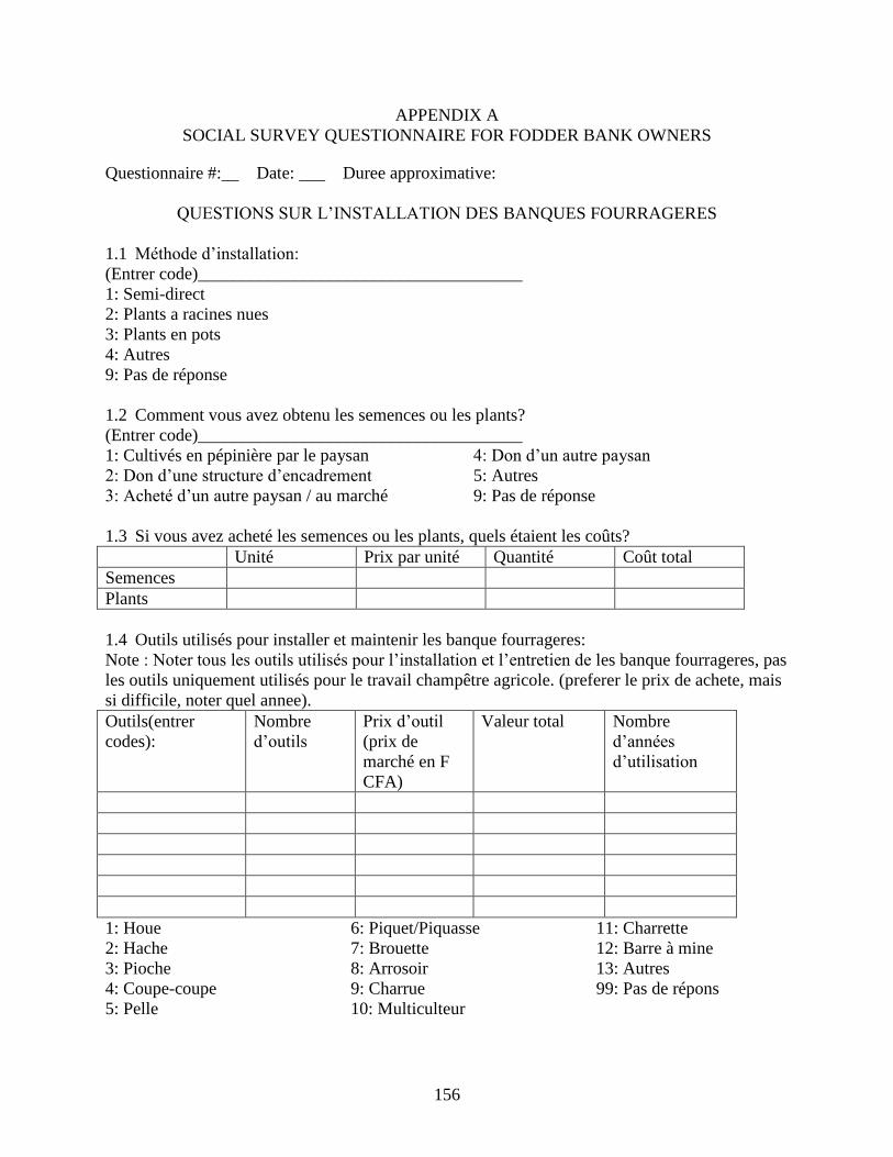
156
APPENDIX A
SOCIAL SURVEY QUESTIONNAIRE FOR FODDER BANK OWNERS
Questionnaire #: Date: Duree approximative:
QUESTIONS SUR L‘INSTALLATION DES BANQUES FOURRAGERES
1.1 Méthode d‘installation:
(Entrer code)_____________________________________
1: Semi-direct
2: Plants a racines nues
3: Plants en pots
4: Autres
9: Pas de réponse
1.2 Comment vous avez obtenu les semences ou les plants?
(Entrer code)_____________________________________
1: Cultivés en pépinière par le paysan
2: Don d‘une structure d‘encadrement
3: Acheté d‘un autre paysan / au marché
4: Don d‘un autre paysan
5: Autres
9: Pas de réponse
1.3 Si vous avez acheté les semences ou les plants, quels étaient les coûts?
Unité Prix par unité Quantité Coût total
Semences
Plants
1.4 Outils utilisés pour installer et maintenir les banque fourrageres:
Note : Noter tous les outils utilisés pour l‘installation et l‘entretien de les banque fourrageres, pas
les outils uniquement utilisés pour le travail champêtre agricole. (preferer le prix de achete, mais
si difficile, noter quel annee).
Outils(entrer
codes):
Nombre
d‘outils
Prix d‘outil
(prix de
marché en F
CFA)
Valeur total Nombre
d‘années
d‘utilisation
1: Houe
2: Hache
3: Pioche
4: Coupe-coupe
5: Pelle
6: Piquet/Piquasse
7: Brouette
8: Arrosoir
9: Charrue
10: Multiculteur
11: Charrette
12: Barre à mine
13: Autres
99: Pas de répons
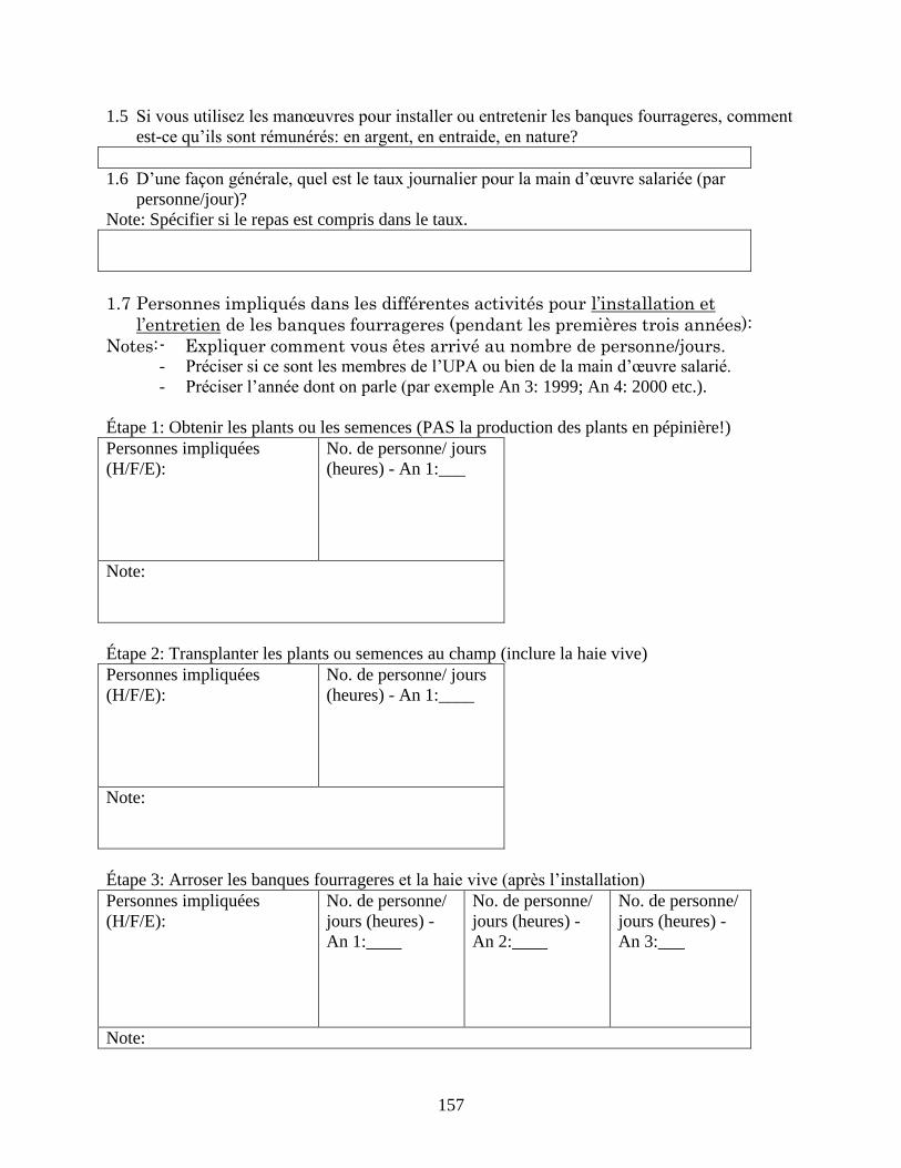
157
1.5 Si vous utilisez les manœuvres pour installer ou entretenir les banques fourrageres, comment
est-ce qu‘ils sont rémunérés: en argent, en entraide, en nature?
1.6 D‘une façon générale, quel est le taux journalier pour la main d‘œuvre salariée (par
personne/jour)?
Note: Spécifier si le repas est compris dans le taux.
1.7 Personnes impliqués dans les différentes activités pour l’installation et
l’entretien de les banques fourrageres (pendant les premières trois années):
Notes: - Expliquer comment vous êtes arrivé au nombre de personne/jours. - Préciser si ce sont les membres de l‘UPA ou bien de la main d‘œuvre salarié.
- Préciser l‘année dont on parle (par exemple An 3: 1999; An 4: 2000 etc.).
Étape 1: Obtenir les plants ou les semences (PAS la production des plants en pépinière!)
Personnes impliquées
(H/F/E):
No. de personne/ jours
(heures) - An 1:___
Note:
Étape 2: Transplanter les plants ou semences au champ (inclure la haie vive)
Personnes impliquées
(H/F/E):
No. de personne/ jours
(heures) - An 1:____
Note:
Étape 3: Arroser les banques fourrageres et la haie vive (après l‘installation)
Personnes impliquées
(H/F/E):
No. de personne/
jours (heures) -
An 1:____
No. de personne/
jours (heures) -
An 2:____
No. de personne/
jours (heures) -
An 3:___
Note:
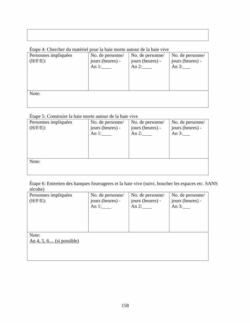
158
Étape 4: Chercher du matériel pour la haie morte autour de la haie vive
Personnes impliquées
(H/F/E):
No. de personne/
jours (heures) -
An 1:____
No. de personne/
jours (heures) -
An 2:____
No. de personne/
jours (heures) -
An 3:___
Note:
Étape 5: Construire la haie morte autour de la haie vive
Personnes impliquées
(H/F/E):
No. de personne/
jours (heures) -
An 1:____
No. de personne/
jours (heures) -
An 2:____
No. de personne/
jours (heures) -
An 3:___
Note:
Étape 6: Entretien des banques fourrageres et la haie vive (suivi, boucher les espaces etc. SANS
récolte)
Personnes impliquées
(H/F/E):
No. de personne/
jours (heures) -
An 1:____
No. de personne/
jours (heures) -
An 2:____
No. de personne/
jours (heures) -
An 3:___
Note:
An 4, 5, 6.... (si possible)
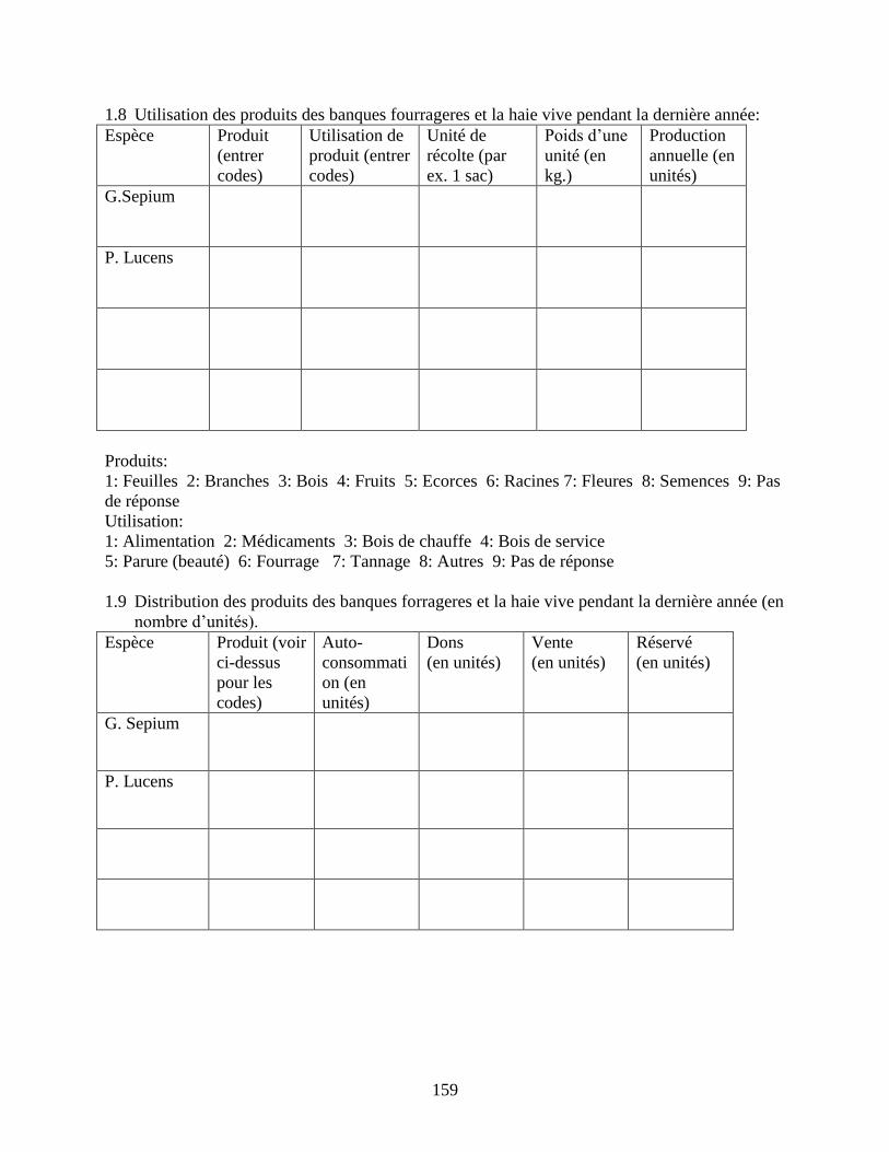
159
1.8 Utilisation des produits des banques fourrageres et la haie vive pendant la dernière année:
Espèce Produit
(entrer
codes)
Utilisation de
produit (entrer
codes)
Unité de
récolte (par
ex. 1 sac)
Poids d‘une
unité (en
kg.)
Production
annuelle (en
unités)
G.Sepium
P. Lucens
Produits:
1: Feuilles 2: Branches 3: Bois 4: Fruits 5: Ecorces 6: Racines 7: Fleures 8: Semences 9: Pas
de réponse
Utilisation:
1: Alimentation 2: Médicaments 3: Bois de chauffe 4: Bois de service
5: Parure (beauté) 6: Fourrage 7: Tannage 8: Autres 9: Pas de réponse
1.9 Distribution des produits des banques forrageres et la haie vive pendant la dernière année (en
nombre d‘unités).
Espèce Produit (voir
ci-dessus
pour les
codes)
Auto-
consommati
on (en
unités)
Dons
(en unités)
Vente
(en unités)
Réservé
(en unités)
G. Sepium
P. Lucens
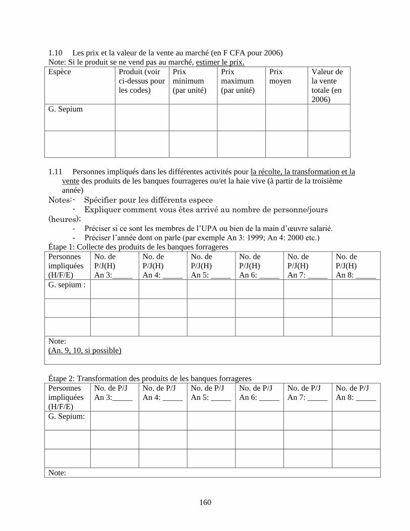
160
1.10 Les prix et la valeur de la vente au marché (en F CFA pour 2006)
Note: Si le produit se ne vend pas au marché, estimer le prix.
Espèce Produit (voir
ci-dessus pour
les codes)
Prix
minimum
(par unité)
Prix
maximum
(par unité)
Prix
moyen
Valeur de
la vente
totale (en
2006)
G. Sepium
1.11 Personnes impliqués dans les différentes activités pour la récolte, la transformation et la
vente des produits de les banques fourrageres ou/et la haie vive (à partir de la troisième
année)
Notes: - Spécifier pour les différents espece
- Expliquer comment vous êtes arrivé au nombre de personne/jours
(heures); - Préciser si ce sont les membres de l‘UPA ou bien de la main d‘œuvre salarié.
- Préciser l‘année dont on parle (par exemple An 3: 1999; An 4: 2000 etc.)
Étape 1: Collecte des produits de les banques forrageres
Personnes
impliquées
(H/F/E)
No. de
P/J(H)
An 3:_____
No. de
P/J(H)
An 4: _____
No. de
P/J(H)
An 5: _____
No. de
P/J(H)
An 6: _____
No. de
P/J(H)
An 7: _____
No. de
P/J(H)
An 8: _____
G. sepium :
Note:
(An. 9, 10, si possible)
Étape 2: Transformation des produits de les banques forrageres
Personnes
impliquées
(H/F/E)
No. de P/J
An 3:_____
No. de P/J
An 4: _____
No. de P/J
An 5: _____
No. de P/J
An 6: _____
No. de P/J
An 7: _____
No. de P/J
An 8: _____
G. Sepium:
Note:
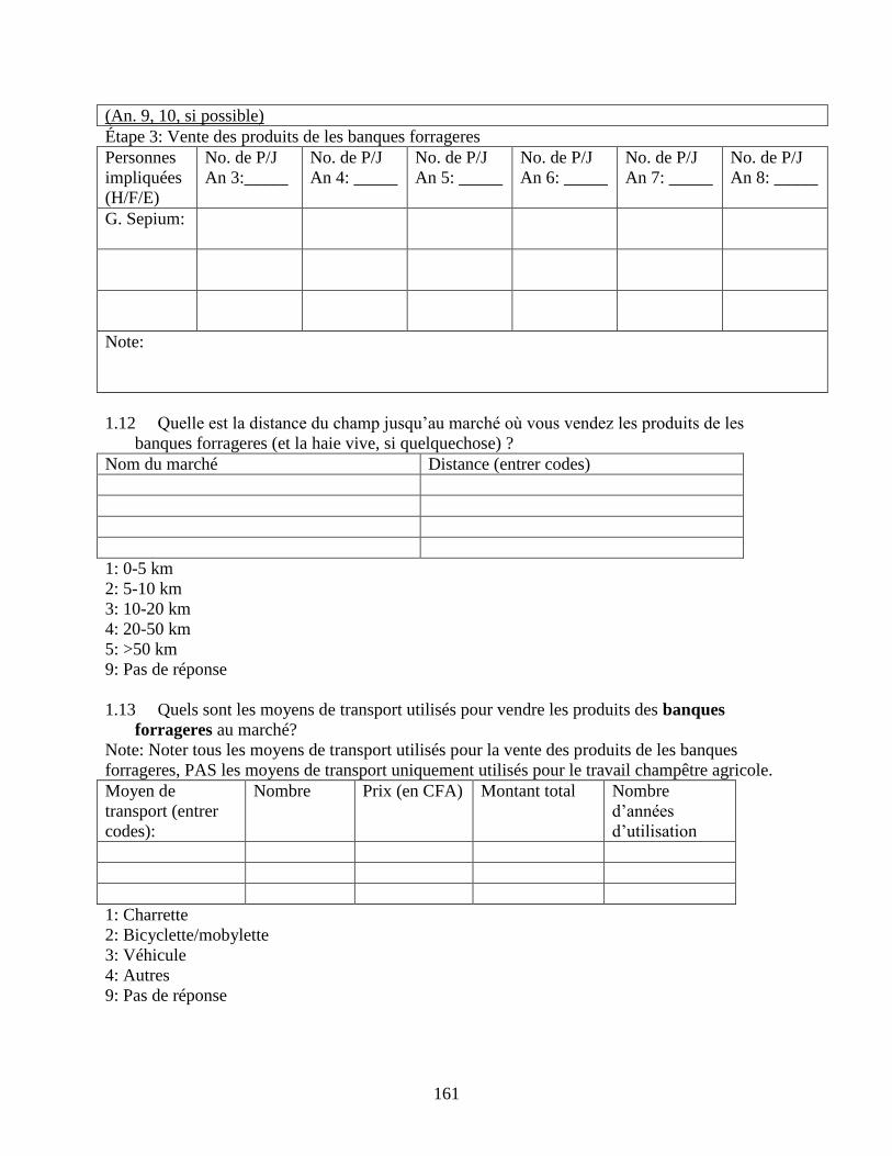
161
(An. 9, 10, si possible)
Étape 3: Vente des produits de les banques forrageres
Personnes
impliquées
(H/F/E)
No. de P/J
An 3:_____
No. de P/J
An 4: _____
No. de P/J
An 5: _____
No. de P/J
An 6: _____
No. de P/J
An 7: _____
No. de P/J
An 8: _____
G. Sepium:
Note:
1.12 Quelle est la distance du champ jusqu‘au marché où vous vendez les produits de les
banques forrageres (et la haie vive, si quelquechose) ?
Nom du marché Distance (entrer codes)
1: 0-5 km
2: 5-10 km
3: 10-20 km
4: 20-50 km
5: >50 km
9: Pas de réponse
1.13 Quels sont les moyens de transport utilisés pour vendre les produits des banques
forrageres au marché?
Note: Noter tous les moyens de transport utilisés pour la vente des produits de les banques
forrageres, PAS les moyens de transport uniquement utilisés pour le travail champêtre agricole.
Moyen de
transport (entrer
codes):
Nombre Prix (en CFA) Montant total Nombre
d‘années
d‘utilisation
1: Charrette
2: Bicyclette/mobylette
3: Véhicule
4: Autres
9: Pas de réponse
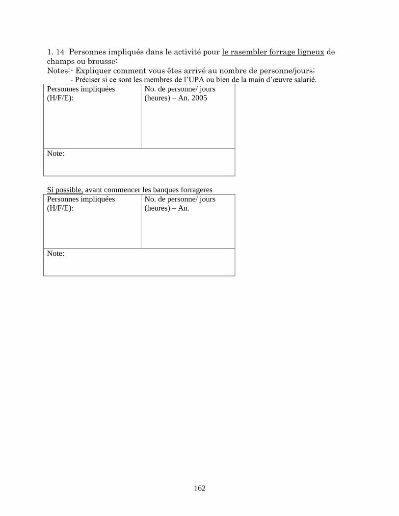
162
1. 14 Personnes impliqués dans le activité pour le rasembler forrage ligneux de
champs ou brousse:
Notes: - Expliquer comment vous êtes arrivé au nombre de personne/jours; - Préciser si ce sont les membres de l‘UPA ou bien de la main d‘œuvre salarié.
Personnes impliquées
(H/F/E):
No. de personne/ jours
(heures) – An. 2005
Note:
Si possible, avant commencer les banques forrageres
Personnes impliquées
(H/F/E):
No. de personne/ jours
(heures) – An.
Note:
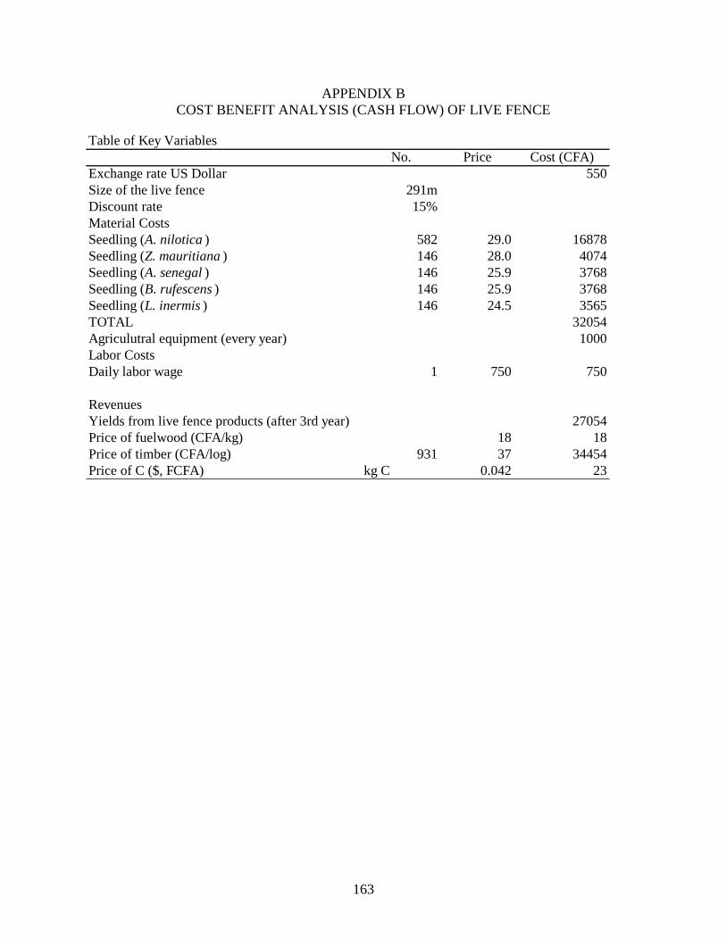
163
APPENDIX B
COST BENEFIT ANALYSIS (CASH FLOW) OF LIVE FENCE
Table of Key Variables
No. Price Cost (CFA)
Exchange rate US Dollar 550
Size of the live fence 291m
Discount rate 15%
Material Costs
Seedling (A. nilotica ) 582 29.0 16878
Seedling (Z. mauritiana ) 146 28.0 4074
Seedling (A. senegal ) 146 25.9 3768
Seedling (B. rufescens ) 146 25.9 3768
Seedling (L. inermis ) 146 24.5 3565
TOTAL 32054
Agriculutral equipment (every year) 1000
Labor Costs
Daily labor wage 1 750 750
Revenues
Yields from live fence products (after 3rd year) 27054
Price of fuelwood (CFA/kg) 18 18
Price of timber (CFA/log) 931 37 34454
Price of C ($, FCFA) kg C 0.042 23
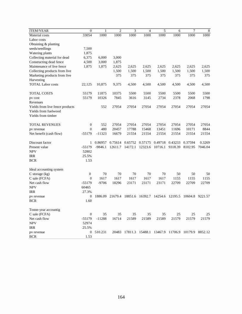
164
ITEM/YEAR 0 1 2 3 4 5 6 7 8
Material costs 33054 1000 1000 1000 1000 1000 1000 1000 1000
Labor costs
Obtaining & planting
seeds/seedlings 7,500
Watering plants 1,875
Collecting material for dead 6,375 6,000 3,000
Constructing dead fence 4,500 3,000 1,875
Maintenance of live fence 1,875 1,875 2,625 2,625 2,625 2,625 2,625 2,625 2,625
Collecting products from live 1,500 1,500 1,500 1,500 1,500 1,500 1,500
Marketing products from live 375 375 375 375 375 375 375
Harvesting
TOTAL Labor costs 22,125 10,875 9,375 4,500 4,500 4,500 4,500 4,500 4,500
TOTAL COSTS 55179 11875 10375 5500 5500 5500 5500 5500 5500
pv cost 55179 10326 7845 3616 3145 2734 2378 2068 1798
Revenues
Yields from live fence products 552 27054 27054 27054 27054 27054 27054 27054
Yields from fuelwood
Yields from timber
TOTAL REVENUES 0 552 27054 27054 27054 27054 27054 27054 27054
pv revenue 0 480 20457 17788 15468 13451 11696 10171 8844
Net benefit (cash flow) -55179 -11323 16679 21554 21554 21554 21554 21554 21554
Discount factor 1 0.86957 0.75614 0.65752 0.57175 0.49718 0.43233 0.37594 0.3269
Present value -55179 -9846.1 12611.7 14172.1 12323.6 10716.1 9318.39 8102.95 7046.04
NPV 52802
IRR 25.5%
BCR 1.53
Ideal accounting system
C storage (kg) 0 70 70 70 70 70 50 50 50
C sale (FCFA) 0 1617 1617 1617 1617 1617 1155 1155 1155
Net cash flow -55179 -9706 18296 23171 23171 23171 22709 22709 22709
NPV 60465
IRR 27.3%
pv revenue 0 1886.09 21679.4 18851.6 16392.7 14254.6 12195.5 10604.8 9221.57
BCR 1.60
Tonne-year accountig
C sale (FCFA) 0 35 35 35 35 35 25 25 25
Net cash flow -55179 -11288 16714 21589 21589 21589 21579 21579 21579
NPV 52974
IRR 25.5%
pv revenue 0 510.231 20483 17811.3 15488.1 13467.9 11706.9 10179.9 8852.12
BCR 1.53
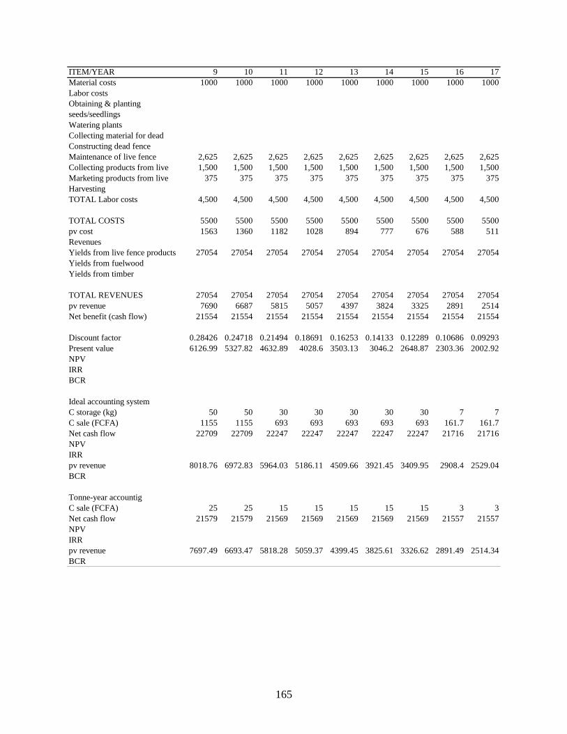
165
ITEM/YEAR 9 10 11 12 13 14 15 16 17
Material costs 1000 1000 1000 1000 1000 1000 1000 1000 1000
Labor costs
Obtaining & planting
seeds/seedlings
Watering plants
Collecting material for dead
Constructing dead fence
Maintenance of live fence 2,625 2,625 2,625 2,625 2,625 2,625 2,625 2,625 2,625
Collecting products from live 1,500 1,500 1,500 1,500 1,500 1,500 1,500 1,500 1,500
Marketing products from live 375 375 375 375 375 375 375 375 375
Harvesting
TOTAL Labor costs 4,500 4,500 4,500 4,500 4,500 4,500 4,500 4,500 4,500
TOTAL COSTS 5500 5500 5500 5500 5500 5500 5500 5500 5500
pv cost 1563 1360 1182 1028 894 777 676 588 511
Revenues
Yields from live fence products 27054 27054 27054 27054 27054 27054 27054 27054 27054
Yields from fuelwood
Yields from timber
TOTAL REVENUES 27054 27054 27054 27054 27054 27054 27054 27054 27054
pv revenue 7690 6687 5815 5057 4397 3824 3325 2891 2514
Net benefit (cash flow) 21554 21554 21554 21554 21554 21554 21554 21554 21554
Discount factor 0.28426 0.24718 0.21494 0.18691 0.16253 0.14133 0.12289 0.10686 0.09293
Present value 6126.99 5327.82 4632.89 4028.6 3503.13 3046.2 2648.87 2303.36 2002.92
NPV
IRR
BCR
Ideal accounting system
C storage (kg) 50 50 30 30 30 30 30 7 7
C sale (FCFA) 1155 1155 693 693 693 693 693 161.7 161.7
Net cash flow 22709 22709 22247 22247 22247 22247 22247 21716 21716
NPV
IRR
pv revenue 8018.76 6972.83 5964.03 5186.11 4509.66 3921.45 3409.95 2908.4 2529.04
BCR
Tonne-year accountig
C sale (FCFA) 25 25 15 15 15 15 15 3 3
Net cash flow 21579 21579 21569 21569 21569 21569 21569 21557 21557
NPV
IRR
pv revenue 7697.49 6693.47 5818.28 5059.37 4399.45 3825.61 3326.62 2891.49 2514.34
BCR
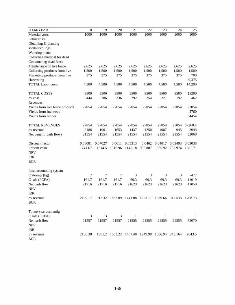
166
ITEM/YEAR 18 19 20 21 22 23 24 25
Material costs 1000 1000 1000 1000 1000 1000 1000 1000
Labor costs
Obtaining & planting
seeds/seedlings
Watering plants
Collecting material for dead
Constructing dead fence
Maintenance of live fence 2,625 2,625 2,625 2,625 2,625 2,625 2,625 2,625
Collecting products from live 1,500 1,500 1,500 1,500 1,500 1,500 1,500 1,500
Marketing products from live 375 375 375 375 375 375 375 700
Harvesting 9,375
TOTAL Labor costs 4,500 4,500 4,500 4,500 4,500 4,500 4,500 14,200
TOTAL COSTS 5500 5500 5500 5500 5500 5500 5500 15200
pv cost 444 386 336 292 254 221 192 462
Revenues
Yields from live fence products 27054 27054 27054 27054 27054 27054 27054 27054
Yields from fuelwood 5760
Yields from timber 34454
TOTAL REVENUES 27054 27054 27054 27054 27054 27054 27054 67268.4
pv revenue 2186 1901 1653 1437 1250 1087 945 2043
Net benefit (cash flow) 21554 21554 21554 21554 21554 21554 21554 52068
Discount factor 0.08081 0.07027 0.0611 0.05313 0.0462 0.04017 0.03493 0.03038
Present value 1741.67 1514.5 1316.96 1145.18 995.807 865.92 752.974 1581.71
NPV
IRR
BCR
Ideal accounting system
C storage (kg) 7 7 7 3 3 3 3 -477
C sale (FCFA) 161.7 161.7 161.7 69.3 69.3 69.3 69.3 -11019
Net cash flow 21716 21716 21716 21623 21623 21623 21623 41050
NPV
IRR
pv revenue 2199.17 1912.32 1662.89 1441.08 1253.11 1089.66 947.533 1708.73
BCR
Tonne-year accountig
C sale (FCFA) 3 3 3 1 1 1 1 1
Net cash flow 21557 21557 21557 21555 21555 21555 21555 52070
NPV
IRR
pv revenue 2186.38 1901.2 1653.22 1437.48 1249.98 1086.94 945.164 2043.5
BCR
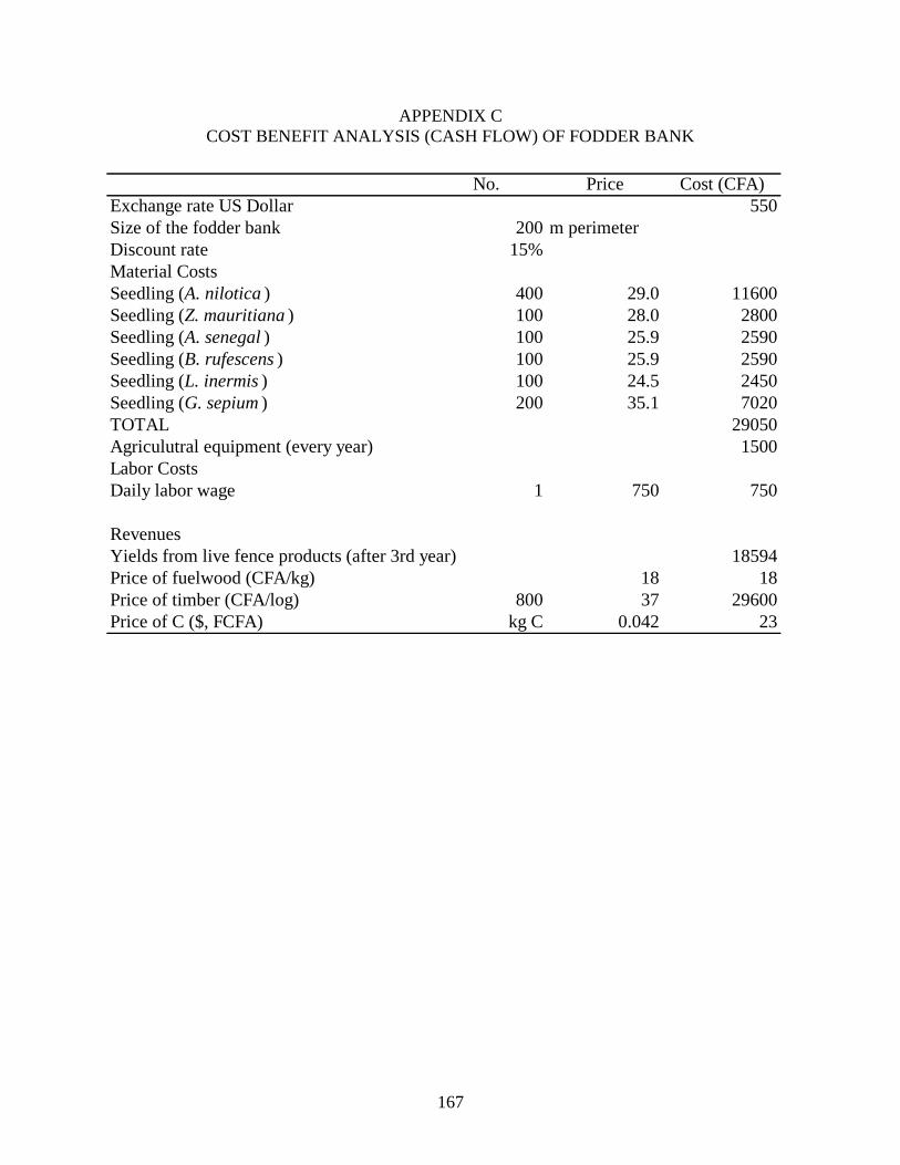
167
APPENDIX C
COST BENEFIT ANALYSIS (CASH FLOW) OF FODDER BANK
No. Price Cost (CFA)
Exchange rate US Dollar 550
Size of the fodder bank 200 m perimeter
Discount rate 15%
Material Costs
Seedling (A. nilotica ) 400 29.0 11600
Seedling (Z. mauritiana ) 100 28.0 2800
Seedling (A. senegal ) 100 25.9 2590
Seedling (B. rufescens ) 100 25.9 2590
Seedling (L. inermis ) 100 24.5 2450
Seedling (G. sepium ) 200 35.1 7020
TOTAL 29050
Agriculutral equipment (every year) 1500
Labor Costs
Daily labor wage 1 750 750
Revenues
Yields from live fence products (after 3rd year) 18594
Price of fuelwood (CFA/kg) 18 18
Price of timber (CFA/log) 800 37 29600
Price of C ($, FCFA) kg C 0.042 23
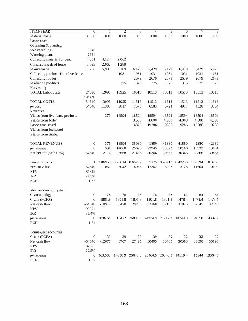
168
ITEM/YEAR 0 1 2 3 4 5 6 7 8
Material costs 30050 1000 1000 1000 1000 1000 1000 1000 1000
Labor costs
Obtaining & planting
seeds/seedlings 8946
Watering plants 2384
Collecting material for dead 4,381 4,124 2,062
Constructing dead fence 3,093 2,062 1,289
Maintenance 5,786 5,909 6,169 6,429 6,429 6,429 6,429 6,429 6,429
Collecting products from live fence 1031 1031 1031 1031 1031 1031 1031
Collecting fodder 2679 2679 2679 2679 2679 2679
Marketing products 375 375 375 375 375 375 375
Harvesting
TOTAL Labor costs 24590 12095 10925 10513 10513 10513 10513 10513 10513
94589
TOTAL COSTS 54640 13095 11925 11513 11513 11513 11513 11513 11513
pv cost 54640 11387 9017 7570 6583 5724 4977 4328 3764
Revenues
Yields from live fence products 379 18594 18594 18594 18594 18594 18594 18594
Yields from foder 3,500 4,000 4,000 4,000 4,500 4,500
Labor time saved 16875 19286 19286 19286 19286 19286
Yields from fuelwood
Yields from timber
TOTAL REVENUES 0 379 18594 38969 41880 41880 41880 42380 42380
pv revenue 0 330 14060 25623 23945 20822 18106 15932 13854
Net benefit (cash flow) -54640 -12716 6668 27456 30366 30366 30366 30866 30866
Discount factor 1 0.86957 0.75614 0.65752 0.57175 0.49718 0.43233 0.37594 0.3269
Present value -54640 -11057 5042 18053 17362 15097 13128 11604 10090
NPV 87319
IRR 29.5%
BCR 1.67
Ideal accounting system
C storage (kg) 0 78 78 78 78 78 64 64 64
C sale (FCFA) 0 1801.8 1801.8 1801.8 1801.8 1801.8 1478.4 1478.4 1478.4
Net cash flow -54640 -10914 8470 29258 32168 32168 31845 32345 32345
NPV 96394
IRR 31.4%
pv revenue 0 1896.68 15422 26807.5 24974.9 21717.3 18744.8 16487.8 14337.2
BCR 1.74
Tonne-year accountig
C sale (FCFA) 0 39 39 39 39 39 32 32 32
Net cash flow -54640 -12677 6707 27495 30405 30405 30398 30898 30898
NPV 87523
IRR 29.5%
pv revenue 0 363.583 14088.9 25648.3 23966.9 20840.8 18119.4 15944 13864.3
BCR 1.67
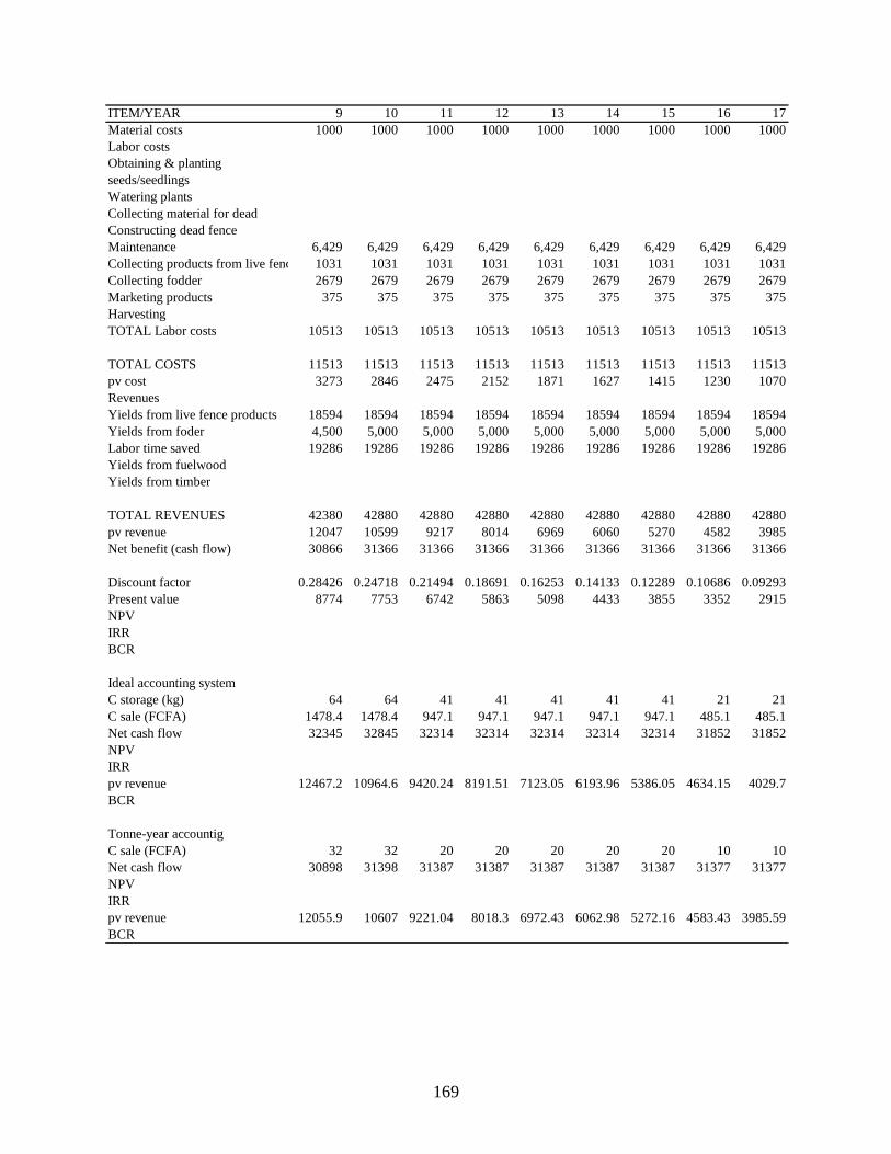
169
ITEM/YEAR 9 10 11 12 13 14 15 16 17
Material costs 1000 1000 1000 1000 1000 1000 1000 1000 1000
Labor costs
Obtaining & planting
seeds/seedlings
Watering plants
Collecting material for dead
Constructing dead fence
Maintenance 6,429 6,429 6,429 6,429 6,429 6,429 6,429 6,429 6,429
Collecting products from live fence 1031 1031 1031 1031 1031 1031 1031 1031 1031
Collecting fodder 2679 2679 2679 2679 2679 2679 2679 2679 2679
Marketing products 375 375 375 375 375 375 375 375 375
Harvesting
TOTAL Labor costs 10513 10513 10513 10513 10513 10513 10513 10513 10513
TOTAL COSTS 11513 11513 11513 11513 11513 11513 11513 11513 11513
pv cost 3273 2846 2475 2152 1871 1627 1415 1230 1070
Revenues
Yields from live fence products 18594 18594 18594 18594 18594 18594 18594 18594 18594
Yields from foder 4,500 5,000 5,000 5,000 5,000 5,000 5,000 5,000 5,000
Labor time saved 19286 19286 19286 19286 19286 19286 19286 19286 19286
Yields from fuelwood
Yields from timber
TOTAL REVENUES 42380 42880 42880 42880 42880 42880 42880 42880 42880
pv revenue 12047 10599 9217 8014 6969 6060 5270 4582 3985
Net benefit (cash flow) 30866 31366 31366 31366 31366 31366 31366 31366 31366
Discount factor 0.28426 0.24718 0.21494 0.18691 0.16253 0.14133 0.12289 0.10686 0.09293
Present value 8774 7753 6742 5863 5098 4433 3855 3352 2915
NPV
IRR
BCR
Ideal accounting system
C storage (kg) 64 64 41 41 41 41 41 21 21
C sale (FCFA) 1478.4 1478.4 947.1 947.1 947.1 947.1 947.1 485.1 485.1
Net cash flow 32345 32845 32314 32314 32314 32314 32314 31852 31852
NPV
IRR
pv revenue 12467.2 10964.6 9420.24 8191.51 7123.05 6193.96 5386.05 4634.15 4029.7
BCR
Tonne-year accountig
C sale (FCFA) 32 32 20 20 20 20 20 10 10
Net cash flow 30898 31398 31387 31387 31387 31387 31387 31377 31377
NPV
IRR
pv revenue 12055.9 10607 9221.04 8018.3 6972.43 6062.98 5272.16 4583.43 3985.59
BCR
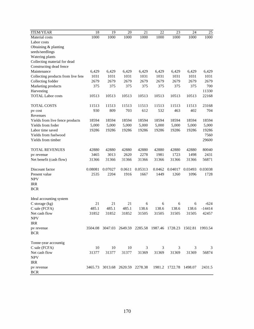
170
ITEM/YEAR 18 19 20 21 22 23 24 25
Material costs 1000 1000 1000 1000 1000 1000 1000 1000
Labor costs
Obtaining & planting
seeds/seedlings
Watering plants
Collecting material for dead
Constructing dead fence
Maintenance 6,429 6,429 6,429 6,429 6,429 6,429 6,429 6,429
Collecting products from live fence 1031 1031 1031 1031 1031 1031 1031 1031
Collecting fodder 2679 2679 2679 2679 2679 2679 2679 2679
Marketing products 375 375 375 375 375 375 375 700
Harvesting 11330
TOTAL Labor costs 10513 10513 10513 10513 10513 10513 10513 22168
TOTAL COSTS 11513 11513 11513 11513 11513 11513 11513 23168
pv cost 930 809 703 612 532 463 402 704
Revenues
Yields from live fence products 18594 18594 18594 18594 18594 18594 18594 18594
Yields from foder 5,000 5,000 5,000 5,000 5,000 5,000 5,000 5,000
Labor time saved 19286 19286 19286 19286 19286 19286 19286 19286
Yields from fuelwood 7560
Yields from timber 29600
TOTAL REVENUES 42880 42880 42880 42880 42880 42880 42880 80040
pv revenue 3465 3013 2620 2278 1981 1723 1498 2431
Net benefit (cash flow) 31366 31366 31366 31366 31366 31366 31366 56871
Discount factor 0.08081 0.07027 0.0611 0.05313 0.0462 0.04017 0.03493 0.03038
Present value 2535 2204 1916 1667 1449 1260 1096 1728
NPV
IRR
BCR
Ideal accounting system
C storage (kg) 21 21 21 6 6 6 6 -624
C sale (FCFA) 485.1 485.1 485.1 138.6 138.6 138.6 138.6 -14414
Net cash flow 31852 31852 31852 31505 31505 31505 31505 42457
NPV
IRR
pv revenue 3504.08 3047.03 2649.59 2285.58 1987.46 1728.23 1502.81 1993.54
BCR
Tonne-year accountig
C sale (FCFA) 10 10 10 3 3 3 3 3
Net cash flow 31377 31377 31377 31369 31369 31369 31369 56874
NPV
IRR
pv revenue 3465.73 3013.68 2620.59 2278.38 1981.2 1722.78 1498.07 2431.5
BCR
171
LIST OF REFERENCES
Alavalapati, J.R.R., R.K. Shrestha, G.A. Stainback, and J.R. Matta. 2004. Agroforestry
development: An environmental economic perspective. Agrofor. Syst. 61-62: 299-310.
Albrecht, A. and S.T. Kandji. 2003. Carbon sequestration in tropical agroforestry systems. Agric.
Ecosyst. Environ. 99:15-27.
Alvarez R., R.A. Diaz, N. Barbero, O.J. Santanatoglia, and L. Blotta. 1995. Soil organic carbon,
microbial biomass and CO2-C production from three tillage systems. Soil Tillage Res. 33:
17-28.
Alvarez, R. and C. R. Alvarez. 2000. Soil organic matter pools and their associations with carbon
mineralization kinetics. Soil Sci. Soc. Am. J. 64:184-189.
Balesdent, J. and A. Mariotti. 1996. Measurement of soil organic matter turnover using 13C
natural abundance. p.83-112. In T.W. Boutton and S.I. Yamasaki (ed.) Mass spectrometry
of soils. Marcel Dekker, New York.
Balesdent, J., E. Besnard, D. Arrouays, and C. Chenu. 1998. The dynamics of carbon in particle-
size fractions of soil in a forest-cultivation sequence. Plant Soil 201:49-57.
Baron, R. and A. Lanza. 2000. Kyoto commitments: macro and micro insights on trading and the
Clean Development Mechanism. Integrated Assessment 1:137-144.
Bationo, A. and B.R. Ntare. 2000. Rotation and nitrogen fertilizer effects on pearl millet, cowpea
and groundnut yield and soil chemical properties in a sandy soil in the semi-arid tropics,
West Africa. J. Agric. Sci.(Cambridge) 134:277-284.
Batjes, N.H. 2004. Estimation of soil carbon gains upon improved management within croplands
and grasslands of Africa. Environ. Dev. Sust. 6:133-143.
Batjes, N.H. 2001. Options for increasing carbon sequestration in West African soils: An
exploratory study with special focus on Senegal. Land Deg. Dev. 12:131-142.
Beare, M. H. , M. L. Cabrera, P. F. Hendrix, and D. C. Coleman. 1994. Aggregate-protected and
unprotected organic matter pools in conventional- and no-tillage soils. Soil Sci. Soc. Am.
J. 58:787-795.
Beer, J., A. Bonnemann, W. Chavez, H.W. Fassbender, A.C. Imbach, and I. Martel. 1990.
Modelling agroforestry systems of cacao (Theobroma cacao) with laurel (Cordia
alliodora) or poro (Erythrina poeppigiana) in Costa Rica. Agrofor. Syst. 12:229-249.
Blair, G.J., R.D.B. Lefroy, and L. Lisle. 1995. Soil carbon fractions based on their degree of
oxidation, and the development of a carbon management index for agricultural systems.
Aust. J. Agric. Res. 46:1459-1466.
172
Boffa, J. M. Agroforestry parklands in sub-Saharan Africa . 1999. FAO Conservation Guides 34.
FAO, Rome, Italy.
Bouliere, F. 1983. Tropical Savannas. Elsevier Scientific Publishing Co. New York, NY.
Breman, H. and J.J. Kessler. 1997. The potential benefits of agroforestry in the Sahel and other
semi-arid regions. Euro. J. Agron. 7:25-33.
Brown, S. 1997. Estimating Biomass and Biomass Change of Tropical Forests: a Primer. FAO,
Rome, Italy.
Brown, S. 1999. Guidelines for Inventorying and Monitoring Carbon Offsets in Forest-Based
Projects. Winrock International, Arlington, VA.
Brown, S. 2002. Measuring carbon in forests: current status and future challenges. Environ.
Pollut. 116:363-372.
Buresh, R.J. and G. Tian. 1997. Soil improvement by trees in sub-Saharan Africa. Agrofor. Syst.
38:51-76.
Cacho, O.J., G.R. Marshall, and M. Milne. 2003a. Smallhoder agroforestry projects: potential for
carbon sequestration and poverty alleviation. ESA Working Paper No.03-06. FAO.
www.fao.org/es/esa
Cacho, O.J., R.L. Hean, and R.M. Wise. 2003b. Carbon-accounting methods and reforestation
incentives. Aust. J. Agric. Res. Econ. 47:153-179.
Cairns, M.A., S. Brown, E.H. Helmer, and G.A. Baumgardner. 1997. Root biomass allocation in
the world's upland forests. Oecologia (Berlin) 111:1-11.
Campbell C.A., B.G. McConkey, R.P. Zentner, F. Selles, and D. Curtin.1996. Tillage and crop
rotation effects on soil organic C and N in a course-textured Typic Haploboroll in
southwestern Saskatchewan. Soil Tillage Res. 37: 3-14.
Campbell, H.A. and P.C. Brown. (ed.) 2003. Benefit-cost analysis: Financial and economic
appraisal using spreadsheets. Cambridge University Press, Port Melbourne, Australia.
Choudhary, M.A., A. Akramkhanov, and S. Saggar. 2002. Nitrous oxide emissions from a New
Zealand cropped soil: tillage effects, spatial and seasonal variability. Agric. Ecosyst.
Environ. 93:33-43.
CIA. 2007. The World Factbook: Mali.[Online] Available at
https://www.cia.gov/library/publications/the-world-factbook/geos/ml.html (verified 5 Jul.
2007). CIA, Washington, DC.
Cisseé, M.I. 1980. Production fourragre de quelques arbres saheliens: relations entre la biomasse
foliaire maximale et divers parametresphysiques. p.203-208. In H.N. Le Houerou. (ed.) Les
fourrages ligneux en Afrique, L‘etat actuel des connaissances. CiPEAA, Addis Abeba.
173
Cissé, M.I. Les parcs agroforestiers au Mali. 1995. Etat des connaissances et perspectives pour
leur amélioration. Rapport AFRENA. ICRAF, Nairobi, Kenya.
Coughenour, M.B., J.E. Ellis, and R.G. Popp. 1990. Morphometric relationships and
developmental patterns of Acacia tortilis and Acacia reficiens in Southern Turkana, Kenya.
Bull. Torrey Bot. Club 117:8-17.
Dai, A., P.J. Lamb, K.E. Trenberth, M. Hulme, P.D. Jones, and P. Xie. 2004. The recent Sahel
drought is real. Int. J. Climat. 24:1323-1331.
Dalsted, N.L. and P.H. Gutierrez. 2007. Partial budgeting. [Online]. Available at
http://www.ext.colostate.edu/PUBS/farmmgt/03760.html (verified 5 Jul. 2007). Colorado
State University Extension-Agriculture, Fort Collins, CO.
De Alwis, K.A. Recapitalization of soil productivity in sub-Saharan Africa. 1996. FAO
Investment Center, Rome, Italy.
De Jong, B.H., S.O. Gaona, S.Q. Montalvo, E.E. Bazan, and N.P. Hernandez. 2004. Economics
of agroforestry carbon sequestration: A case study from southern Mexico. Chap.4. In
J.R.R. Alavalapati and D.E. Mercer (ed.) Valuing agroforestry systems. Kluwer Academic
Publishers, Netherlands.
De Jong, B.H.J. 2001. Uncertainties in estimating the potential for carbon mitigation of forest
management. For. Ecol. Manage. 154:85-104.
Del Galdo, I., J. Six, A. Peressotti, and M.F. Cotrufo. 2003. Assessing the impact of land-use
change on soil C sequestration in agricultural soils by means of organic matter
fractionation and stable C isotopes. Glob. Chan. Bio. 9:1204-1213.
Delaney, M. and J. Roshetko. 1999. Field test of carbon monitoring methods for home gardens in
Indonesia p.45-51. In Field Tests of Carbon Monitoring Methods in Forestry Projects.
Forest Carbon Monitoring Program. Winrock International, Arlington, VA.
Denton, F., Y. Sokona, and J.P. Thomas. Climate change and sustainable development strategies
in the making: What should West African countries expect? 2001. OECD Climate Change
and Development. Environnement et Développement du Tiers Monde (ENDA-TM),
Dakar, Senegal.
Dixon, R.K. 1995. Agroforestry system: sources or sinks of greenhouse gases? Agrofor. Syst.
31:99-116.
Dixon, R.K., S Brown, R.A. Houghton, M.C. Solomon, M.C. Trexler, and J. Wisniewski. 1994a
Carbon pools and flux of global forest ecosystems. Science (Washington, DC) 263:185-
190.
Dixon, R.K., J.K. Winjum, K.J. Andrasko, J.J. Lee, and P.E. Schroeder. 1994b. Integrated land-
use systems: assessment of promising agroforest and alternative land-use practices to
enhance carbon conservation and sequestration. Clim. Change 27:71-92.
174
Doumbia, O. Final Report on the Soil Resources of the Villages Covered by the ―JICA-SEGOU
Project‖ 2000. Ségou, Mali.
Droppelmann, K.J., J. Lehmann, J.E. Ephrath, and P.R. Berliner. 2000. Water use efficiency and
uptake patterns in a runoff agroforestry system in an arid environment. Agrofor. Syst.
49:223-243.
Duguma, B., J. Gockowski, and J. Bakala. 2001. Smallholder cacao (Theobroma cacao Linn.)
cultivation in agroforestry systems of West and Central Africa: challenges and
opportunities. Agrofor. Syst. 51:177-188.
Duiker, S.W. and R. Lal. 1999. Crop residue and tillage effects on carbon sequestration in a
Luvisol in central Ohio. Soil Tillage Res. 52, 73-81.
Dzurec, R.S., T.W. Boutton, M.M. Caldwell, and B.N. Smith. 1985. Carbon isotope ratios of soil
organic matter and their use in assessing community composition changes in Curlew
Valley, Utah. Oecologia (Berlin) 66:17-24.
Eleki, K., R.M. Cruse, and K.A. Albrecht. 2005. Root segregation of C3 and C4 species using
carbon isotope composition. Crop Sci 45:879-882.
Eswaran, H., R. Almaraz, E. Berg, and P. Reich. 1996. An Assessment of the Soil Resources of
Africa in Relation to Productivity. [Online] Available at
http://soils.usda.gov/use/worldsoils/papers/africa1.html (verified 5 Jul. 2007). NRCS,
Washington, DC.
FAO. 2000. Global Forest Resources Assessment 2000. FAO Forestry Paper 140. Rome, Italy.
FAO. 1997. Estimating biomass and biomass change of tropical forests. FAO Forestry Paper
134. Rome, Italy.
FAO. 1991. Feeding dairy cows in the tropics. FAO Animal Production and Health Paper 86.
Rome, Italy.
Ferguson, W. 1983. Integrating crops and livestock in West Africa. FAO Animal Production and
Health Paper 41. Rome, Italy.
Franklin, J. and P. Hiernaux. 1991. Estimating foliage and woody biomass in Sahelian and
Sudanian woodlands using a remote sensing model. Int. J. Remote Sens.12:1387-1404.
Franzluebbers, A.J., F.M. Hons, and D.A. Zuberer. 1995. Tillage-induced seasonal changes in
soil physical properties affecting soil CO2 evolution under intensive cropping. Soil Tillage
Res. 34: 41-60.
Garcia-Oliva, F. and O.R. Masera. 2004. Assessment and measurement issues related to soil
carbon sequestration in Land-Use, Land-Use Change, and Forestry (LULUCF) projects
under the Kyoto Protocol. Clim. Change 65:347-364.
175
Gebhart, D.L., H.B. Johnson, H.S. Mayeux, and H.W. Polley. 1994. The CRP increases soil
organic carbon. 49: 488-492. J. Soil Water Conserv.
Ghani, A., M. Dexter, and K.W. Perrott. 2003. Hot-water extractable carbon in soils: a sensitive
measurement for determining impacts of fertilisation, grazing and cultivation. Soil Biol.
Biochem. 35:1231-1243.
Godal, O., Y. Ermoliev, G. Klaassen, and M. Obersteiner. 2003. Carbon trading with imperfectly
observable emissions. Environ. Res. Econ. 25:151-169.
Gonzalez, P. 2001. Desertification and a shift of forest species in the West African Sahel. Clim.
Res. 17:217-228.
Gordon, J.E., W.D. Hawthorne, G. Sandoval, and A.J. Barrance. 2003. Trees and farming in the
dry zone of southern Honduras II: the potential for tree diversity conservation. Agrofor.
Syst. 59:107-117.
Gritzner, J.A. 1988. The West African Sahel. University of Chicago, Committee on
Geographical Studies, Chicago, IL.
Hamer, A., S. Franzel, B. Mounkoro, A. Niang, and C.O. Traore. 2005. Fodder banks in Mali.
ICRAF, Bamako, Mali.
Hardner, J.J., P.C. Frumhoff, and D.C. Goetze. 2000. Prospects for mitigating carbon, conserving
biodiversity, and promoting socioeconomic development objectives through the clean
development mechanism. Mitig. Adapt. Strat. Glob. Change 5:61-80.
Harris, D., R.H. William, and C. van Kessel. 2001. Acid fumigation of soils to remove
carbonates prior to total organic carbon or CARBON-13 isotopic analysis. Soil Sci. Soc.
Am. J. 65:1853-1856.
Hassink, J. 1997. The capacity of soils to preserve organic C and N by their association with clay
and silt particles. Plant Soil 191:77-87.
ICRAF. 2007. ICRAF Position on the Clean Development Mechanism in the Land-Use, Land-
Use Change and Forestry Sector. [Online] Available at
http://www.worldagroforestry.org/climatechange/documents/ICRAFPositiononCDM.pdf
(verified 5 Jul. 2007) Nairobi, Kenya.
ICRISAT. Crops. 2007. [Online] Available at http://www.icrisat.org/ (verified 5 Jul. 2007).
Ingram, J.S.I. and E.C.M. Fernandes. 2001. Managing carbon sequestration in soils: concepts
and terminology. Agric. Ecosys. Environ. 87:111-117.
IPCC. 2007. Climate Change 2007: Mitigation of Climate Change. Working Group III
contribution to the Intergovernmental Panel on Climate Change, Fourth Assessment
Report. Bangkok, Thailand.
176
IPCC. 2000. Land use, Land-use Change, and Forestry. A Special Report of the IPCC.
Cambridge University Press Cambridge, UK.
Jeltsch, F., S.J. Milton, W.R.J. Dean, and N. van Rooyen. 1996. Tree spacing and coexistence in
semiarid savannas. J. Ecol. 84:583-595.
Jobbagy, E.G. and R.B. Jackson. 2000. The vertical distribution of soil organic carbon and its
relation to climate and vegetation. Ecol. Applic. 10:423-436.
Johnsen, K.H., D. Wear, R. Oren, R.O. Teskey, F. Sanchez, R. Will, J. Butnor, D. Markewitz, D.
Richter, T. Rials, H.L. Allen, J. Seiler, D. Ellsworth, C. Maier, G. Katul, and P.M.
Dougherty. 2001. Meeting global policy commitments: Carbon sequestration and southern
pine forests. J. For. 99:14-21.
Jones, M., M.L. Sinclair, and V.L. Grime. 1998. Effect of tree species and crown pruning on root
length and soil water content in semi-arid agroforestry. Plant Soil. 201:197-207.
Jonsson, K., C.K. Ong, and J.C.W. Odongo. 1999. Influence of scattered Nere and Karite trees
on microclimate, soil fertility and millet yield in Burkina Faso. Exp. Agric. 35:39-53.
Kang, B.T., F.E. Caveness, G. Tian, and G.O. Kolawole. 1999. Longterm alley cropping with
four hedgerow species on an Alfisol in southwestern Nigeria – effect on crop performance,
soil chemical properties and nematode population. Nutr. Cycl. Agroecosyst. 54:145-155.
Kater, L.J.M., S. Kante, and A Budelman. 1992. Karite (Vitellaria paradoxa) and nere(Parkia
biglobosa) associated with crops in South Mali. Agrofor. Syst. 18:89-105.
Kaya, B. 2000. Soil fertility regeneration through improved fallow systems in southern Mali.
Ph.D. diss.Univ. of Florida, Gainesville, FL.
Kaya, B. and P.K.R. Nair. 2004. Dynamics of Particulate Organic Matter following biomass
addition from fallow-improvement species in southern Mali. Agrofor. Syst. 60:267-276.
Kaya, B. and P.K.R. Nair. 2001. Soil fertility and crop yields under improved-fallow systems in
southern Mali. Agrofor. Syst. 52:1-11.
Klemperer, W.D. (ed.) 1996. Forest resource economics and finance. McGraw-Hill, Inc, USA.
Kursten, E. and P. Burschel. 1993. CO2-mitigation by agroforestry. Water Air Soil Pollut.
70:533-544.
Lal, R. 2004a. Carbon sequestration in dryland ecosystems. Environ. Manag. 33:528-544 .
Lal, R. 2004b. Soil carbon sequestration impacts on global climate change and food security.
Science (Washington, DC) 304:1623-1627.
177
Lal, R. 1999. Global carbon pools and fluxes and the impact of agricultural intensification and
judicious land use. p. 44-52. In Prevention of Land Degradation, Enhancement of Carbon
Sequestration and Conservation of Biodiversity through Land Use Change and Sustainable
Land Management with a Focus on Latin America and the Caribbean. FAO, Rome, Italy.
Levasseur, V., M. Djimde, and A. Olivier. 2004. Live fences in Ségou, Mali: an evaluation by
their early users. Agrofor. Syst. 60:131-136.
Littmann, T. 1991. Rainfall, temperature, and dust storm anomalities in the African Sahel.
Geogr. J 157:136-160.
MacDicken, K.G. (ed.) 1997. A guide to monitoring carbon storage in forestry and agroforestry
projects. Winrock International Institute for Agricultural Development, Forest Carbon
Monitoring Program. Arlington, VA.
Makumba, W., B. Janssen, O. Oenema, F.K. Akinnifesi, D. Mweta, and F. Kwesiga. 2006. The
long-term effects of a gliricidia-maize intercropping system in Southern Malawi, on
gliricidia and maize yields, and soil properties: Nutrient management in tropical
agroecosystems. Agric. Ecosyst. Environ. 116:85-92.
Makundi, W.R. and J.A. Sathaye. 2004. GHG Mitigation potential and cost in tropical forestry -
relative role for agroforestry. Environ. Dev. Sust. 6:235-260.
Manlay, R.J., J.L. Chotte, D. Masse, J.Y. Laurent, and C. Feller. 2002. Carbon, nitrogen and
phosphorus allocation in agro-ecosystems of a West African savanna: III. Plant and soil
components under continuous cultivation. Agric. Ecosyst. Environ. 88:249-269.
Marino, B.D. and M.B. McElroy. 1991. Isotopic composition of atmospheric CO2 inferred from
carbon in C4 plant cellulose. Nature 349:127.
Masera, O.R., J.F. Garza-Caligaris, M. Kanninen, T. Karjalainen, J. Liski, G.J. Nabuurs, A.
Pussinen, B.H.J. de Jong, and G.M.J. Mohren. 2003. Modeling carbon sequestration in
afforestation, agroforestry and forest management projects: the CO2FIX V.2 approach.
Ecol. Modell. 164:177-199.
McDonagh, J.F., T.B.Thomsen, and J. Magid. 2001. Soil organic matter decline and
compositional change associated with cereal cropping in southern Tanzania. Land Deg.
Dev. 12:13-26.
McLauchlan, K.K. and S.E. Hobbie. 2004. Comparison of labile soil organic matter fractionation
techniques. Soil Sci. Soc. Am. J. 68:1616-1625.
Mitchell, T. 2005. Sahel rainfall index (20-10N, 20W-10E), 1898 – 2004. [Online] Avaliable at
http://jisao.washington.edu/data_sets/sahel/index2.html#values (verified 5 Jul. 2007).
University of Washington, Seattle, WA.
Montagnini, F. and P.K.R. Nair. 2004. Carbon sequestration: An underexploited environmental
benefit of agroforestry systems. Agrofor. Syst. 61-62:281-295.
178
Moody, P.W., S.A. Yo, and R.L. Aitken. 1997. Soil organic carbon, permanganate fractions, and
the chemical properties of acidic soils. Aust. J. Soil Res. 35:1301-1308.
Mosier, A., R. Wassmann, L. Verchot, J. King, and C. Palm. 2004. Methane and nitrogen oxide
fluxes in tropical agricultural soils: Sources, sinks and mechanisms. Environ. Dev. Sust.
6:11-49.
Moura-Costa, P. and C. Wilson. 2000. An equivalence factor between CO2 avoidedemissions
and sequestration – description and applications in forestry. Mitig. Adapt. Strat. Glob.
Change 5:51-60.
Nair, P. K. R. and V.D. Nair. 2003. Carbon storage in North American agroforestry systems. In:
Kimble, J., Heath, L.S., Birdsey, R.A., and Lal, R. (eds). The Potential of U.S. Forest Soils
to Sequester Carbon and Mitigate the Greenhouse Effect, pp. 333-346. CRC Press LLC,
Boca Raton, FL.
Nair, P.K.R. (ed.) 1993. An Introduction to Agroforestry. Kluwer Academic Publishers,
Dordrecht, Netherlands.
Niang, A., M. Djimde, B. Kaya, E.G. Bonkoungou, and M. Macalou. 2002. Paper presented at
Improving the quantity and quality of dry season fodder availability in the Sahel. Presented
at the Regional Agroforestry Conference. Pretoria, South Africa. May 20-24, 2002.
Nierop, K.G.J., F.H. Tonneijck, B. Jansen, and J.M. Verstraten. 2007. Organic matter in volcanic
ash soils under forest and paramo along an Ecuadorian altitudinal transect. Soil Sci. Soc.
Am. J. 71:1119-1127.
Oba, N., N.C. Stenseth, and W.J. Lusigi. 2000. New perspectives on sustainable grazing
management in arid zones of sub-Saharan Africa. Bioscience 50:35-51.
Onim, J.F.M., M. Mathuva, K. Otieno, and H.A. Fitzhugh. 1990. Soil fertility changes and
response of maize and beans to green manures of leucaena, sesbania and pigeonpea.
Agrofor. Syst. 12:197-215.
Oren, R., D.S. Ellsworth, K.H. Johnsen, N. Phillips, B.E. Ewers, C. Maier, K.V.R Schafer, H.
McCarthy, G. Hendrey, S.G. McNulty, and G.G Katul. 2001. Soil fertility limits carbon
sequestration by forest ecosystems in a CO2-enriched atmosphere. Nature (London)
411:469-472.
Palm, C.A, T. Tomich, M. Van Noordwijk, S. Vosti, J. Alegre, J. Gockowski, and L. Verchot.
2004. Mitigating GHG emissions in the humid tropics: Case studies from the Alternatives
to Slash-and-Burn Program (ASB). Environ. Dev. Sust. 6:145-162.
179
Palm, C.A., P.L. Woomer, J. Alegre, L. Arevalo, C. Castilla, D.G. Cordeiro, B. Feigl, K. Hairiah,
J. Kotto-Same, A. Mendes, A. Moukam, D. Murdiyarso, R. Njomgang, W.J. Parton, A.
Ricse, V. Rodrigues, S.M. Sitompul, and M van Noordwijk. 1999. Carbon sequestration
and trace gas emissions in slash and burn and alternative land use in the humid tropics.
ASB Climate Change Working Group Final Report, Phase II. ASB Coordination Office,
ICRAF, Nairobi, Kenya.
Paustian, K., O. Andren, H.H. Janzen, R. Lal, P. Smith, G. Tian, H. Tiessen, M. van Noordwijk,
and P. L. Woomer. 1997. Agricultural soils as a sink to mitigate CO2 emissions. Soil Use
and Manage. 13: 230-244.
Pfaff, A.S.P., S. Kerr, R.F. Hughes, S. Liu, G.A. Sanchez-Azofeifa, D. Schimel, J. Tosi, and V.
Watson. 2000. The Kyoto protocol and payments for tropical forest: An interdisciplinary
method for estimating carbon-offset supply and increasing the feasibility of a carbon
market under the CDM. Ecol. Econ. 35:203-221.
Phillips, D.L., P.D. Hardin, V.W. Benson, J.V. Baglio. 1993. Nonpoint source pollution impacts
of alternative agricultural management practices in Illinois: A simulation study. J. Soil
Water Consev. 48: 449-457.
Pikul, J.L., S. Osborne, M. Ellsbury, and W. Riedell. 2007. Particulate organic matter and water-
stable aggregation of soil under contrasting management. Soil Sci. Soc. Am. J. 71:766-776.
Post, W. M. and K.C. Kwon. 2000. Soil carbon sequestration and land-use change: processes and
potential. Glob. Change Biol. 6:317-327.
Potvin, C., E. Whidden, and T. Moore. 2004. A case study of carbon pools under three different
land-uses in Panama. Clim. Change 67:291-307.
Powers, J.S. and E. Veldkamp. 2005. Regional variation in soil carbon and 13C in forests and
pastures of northeastern Costa Rica. Biogeochem. 72:315-336.
Powers, J.S. and W.H. Schlesinger. 2002. Relationships among soil carbon distributions and
biophysical factors at nested spatial scales in rain forests of northeastern Costa Rica.
Geoderma 109:165-190.
ProKarite. Projet d‘Appui Technique à la Fillière Karité 2007. [Online] Available at
http://www.prokarite.org/index-eng.html (verified 5 Jul.2007). Bamako, Mali.
Reich, P.F., S.T. Numbrem, R.A. Almaraz, and H. Eswaran. 2001. Land resource stresses and
desertification in Africa. In E.M. Bridges, I.D. Hannam, L.R. Oldeman, F.W.T. Pening de
Vries, S.J. Scherr, and S. Sompatpanit (eds.). Responses to Land Degradation. Proc. 2nd.
International Conference on Land Degradation and Desertification, Khon Kaen, Thailand.
Oxford Press, New Delhi, India.
République du Mali. 2005. Minitere du Plan et de L amenagement du Territoire and Ministere de
L agriculture de L elevage et de la Peche. Enquete Agricole de Conjoncture Campagne
2003/2004. Bamako, Mali.
180
Rhoton, F.E. 2000. Influence of time on soil response to no-till practices. Soil Sci. Soc. Am. J.
64: 700-709.
Richter, D.D., D. Markewitz, S.E. Trumbore, and C.G. Wells. 1999. Rapid accumulation and
turnover of soil carbon in a re-establishing forest. Nature (London) 400:56-58.
Ringius, L. 2002. Soil carbon sequestration and the CDM: Opportunities and challenges for
Africa. Clim. Change 54:471-495.
Roose, E., V. Kabore, and C. Guenat. 1999. Zai Practice: A west African traditional
rehabilitation system for semiarid degraded lands, a case study in Burkina Faso. Arid Soil
Res. Rehabil. 13:343-355.
Rosalina, U., Setiabudhi, and A.E. Putra. Vegetation analysis and database management system
in Lampung and Jambi. 1997. ICRAF Southeast Asia Regional Office, Bogor, Indonesia.
Rose, S., H. Ahammad, B. Eickhout, B. Fisher, A. Kurosawa, S. Rao, K. Riahi, and D. van
Vuuren. 2007. Land in climate stabilization modeling: Initial observations. [Online]
Available at http://www.stanford.edu/group/EMF/projects/group21/Landuse.pdf (verified 5
Jul. 2007). Stanford Energy Modeling Forum (EMF), Stanford University, Stanford, CA.
Roshetko, J.M., M. Delaney, K. Hairiah, and P Purnomosidhi. 2002. Carbon stocks in Indonesian
homegarden systems: Can smallholder systems be targeted for increased carbon storage?
Am. J. Alt. Agric. 17:138-148.
Sathaye, J.A., W.R. Makundi, K. Andrasko, R. Boer, N.H. Ravindranath, P. Sudha, S. Rao, R.
Lasco, F. Pulhin, O. Masera, A. Ceron, J. Ordonez, X. Deying, X. Zhang, and S. Zuomin.
2001. Carbon mitigation potential and costs of forestry options in Brazil, China, India,
Indonesia, Mexico, the Philippines and Tanzania. Mitig. Adapt. Strat. Glob. Change
6:185-211.
Schimel, D.S., B.H. Braswell, E.A. Holland, R. McKeown, D.S. Ojima, T.H. Painter, W.J.
Parton, and A.R. Townsend. 1994. Climatic, edaphic, and biotic controls over storage and
turnover of carbon in soils. Glob. Biogeochem. Cycl. 8:279-293.
Schroeder, P. 1994. Carbon storage benefits of agroforestry systems. Agrofor. Syst. 27:89-97.
Schroth, G., S.A. D'Angelo, W.G. Teixeira, D. Haag, and R. Lieberei. 2002. Conversion of
secondary forest into agroforestry and monoculture plantations in Amazonia: consequences
for biomass, litter and soil carbon stocks after 7 years. For. Ecol. Manag. 163:131-150.
Schuur, E.A.G. 2001. The effect of water on decomposition dynamics in mesic to wet Hawaiian
montane forests. Ecosystems 4:259-273.
Scolel Te. 2007. [Online] Available at http://www.eccm.uk.com/scolelte/ (verified 5 Jul. 2007).
Edinburgh, UK.
181
Seghieri, J., M. Simier, A. Mahamane, P. Hiernaux, and S. Rambal. 2005. Adaptative above-
ground biomass, stand density and leaf water potential to droughts and clearing in Guiera
senegalensis, a dominant shrub in Sahelian fallows (Niger). J. Trop. Ecol. 21:203-213.
Sharrow, S.H. and S. Ismail. 2004. Carbon and nitrogen storage in agroforests, tree plantations,
and pastures in western Oregon, USA. Agrofor. Syst. 60:123-130.
Shepherd, D. and F. Montagnini. 2001. Above ground carbon sequestration potential in mixed
and pure tree plantation in the humid tropics. J. Trop. For. Sci. 13:450-459.
Six, J., R.T. Conant, E.A. Paul, and K. Paustian. 2002a. Stabilization mechanisms of soil organic
matter: Implications for C-saturation of soils. Plant Soil 241:155-176.
Six, J., P. Callewaert, S. Lenders, S. De Gryze, S.J. Morris, E.G. Gregorich, E.A. Paul, and K.
Paustian. 2002b. Measuring and understanding carbon storage in afforested soils by
physical fractionation. Soil Sci. Soc. Am. J. 66:1981-1987.
Six, J., R. Merckx, K. Kimpe, K. Paustian, and E.T. Elliott. 2000c. A re-evaluation of the
enriched labile soil organic matter fraction. Eur. J. Soil Sci. 51: 283-293.
Six, J., E.T. Elliott, K. Paustian, and J.W. Doran. 1998. Aggregation and soil organic matter
accumulation in cultivated and native grassland soils. Soil Sci. Soc. Am. J. 62:1367-1377.
Smith, P., D.S. Powlson, M.J. Glending, and J.U. Smith. 1998. Preliminary estimates of the
potential for carbon mitigation in European soils through no-till farming. Glob. Change
Bio. 4: 679-685.
Stainback, A.G. and J.R.R. Alavalapati. 2002. Economic analysis of slash pine forest carbon
sequestration in the southern U.S. J. For. Econ. 8:105-117.
Sun, O.J., J. Campbell, B.E. Law, and V. Wolf. 2004. Dynamics of carbon stocks in soils and
detritus across chronosequences of different forest types in the Pacific Northwest, USA.
Glob. Chan. Biol.10:1470-1481.
Tan, Z.X., R. Lal, N.E. Smeck, and F.G. Calhoun. 2004. Relationships between surface soil
organic carbon pool and site variables. Geoderma 121: 187-195.
Tiepolo, G., M. Calmon, and A.R. Feretti. 2002. Paper presented at measuring and monitoring
carbon stocks at the Guaraquecaba Climate Action Project, Parana, Brazil. Proceedings of
the International Symposium on Forest Carbon Sequestration and Monitoring. 11-15
November 2002, Taipei, Taiwan. Taiwan Forestry Research Institute Winrock
International.
Tiessen, H., H.K. Hauffe, and A.R. Mermut. 1991. Deposition of Harmattan dust and its
influence on base saturation of soils in northern Ghana. Geoderma 49:285-299.
Tieszen, L.L. 1991. Natural variations in the carbon isotope values of plants: implicaations for
archaeology, ecology and paleoecology. J. Archaeol. Sci. 18: 227.
182
Tipper, R. and B.H. De Jong. 1998. Quantification and regulation of carbon offsets from
forestry: comparison of alternative methodologies, with special reference to Chiapas,
Mexico. Commonwealth For. Rev. 77:219-228.
Tomich, T.P., H. de Foresta, R. Dennis, Q. Ketterings , D. Murdiyarso, C. Palm, F. Stolle,
Suyanto, and M. van Noordwijk. 2002. Carbon offsets for conservation and development
in Indonesia? Am. J. Alt. Agric. 17:125-137.
Traore, C.O., F. Place, and A. Niang. 2002. Evaluation economique des couts de production des
plants d'especes haies vives a la pepiniere de Ségou. Mali. ICRAF, Bamako, Mali.
Tschakert, P. 2004. Carbon for farmers: Assessing the potential for soil carbon sequestration in
the Old Peanut Basin of Senegal. Clim. Change 67:273-290.
Tschakert, P. 2007. Environmental services and poverty reduction: Options for smallholders in
the Sahel: Making carbon sequestration work for Africa's rural poor - Opportunities and
constraints. Agric. Syst. 94:75-86.
UNFCCC. 2006. Revised simplified baseline and monitoring methodologies for selected small-
scale afforestation and reforestation project activities under the clean development
mechanism. [Online] Available at
http://cdm.unfccc.int/UserManagement/FileStorage/CDMWF_AM_A3II6AX6KGW5GBB
7M6AI98UD3W59X4 (verified 5 Jul.2007). Bonn, Germany.
UNFCCC 2007. [Online] Available at http://unfccc.int/2860.php (verified 5 Jul.2007). Bonn,
Germany.
USGS. 2007. International Program Sahel Land Use. [Online] Available at
http://edcintl.cr.usgs.gov/sahel.html (verified 5 Jul. 2007). Reston, VA.
Van Dorp, M., B. Mounkoro, S. Soumana, C.O. Traore, S. Franzel, F. Place, and A. Niang. 2005.
Economic analysis of improved live fences as an agroforestry technology as compared to
traditional live fences and dead fences in the Ségou Region, Mali. ICRAF, Bamako, Mali.
Van Duijl, E. 2000. Feeding livestock in the dry season: towards identifying potential adopters
for fodderbanks in Ségou, Mali. Draft Report. ICRAF, Bamako, Mali.
Van Duijl, E.C. 1999. Characterisation of potential adopters for live fences in Ségou, Mali.
ICRAF, Bamako, Mali.
Van Noordwijk, M., S. Rahayu, K. Hairiah, Y.C. Wulan, A. Farida, and B. Verbist. 2002.
Carbon stock assessment for a forest-to-coffee conversion landscape in Sumber-Jaya
(Lampung, Indonesia): from allometric equations to land use change analysis. Science
China 45:75-86.
Walker, S.M. and P.V. Desanker. 2004. The impact of land use on soil carbon in Miombo
Woodlands of Malawi. For. Ecol. Manag. 203:345-360.
183
Wise, R. and O. Cacho. 2005. Tree-crop interactions and their environmental and economic
implications in the presence of carbon-sequestration payments. Environ. Modell. Software
20:1139-1148.
Woomer, P.L., L.L. Tieszen, G. Tappan, A. Toure, and M. Sall. 2004a. Land use change and
terrestrial carbon stocks in Senegal. J. Arid Environ. 59:625-642.
Woomer, P.L., A. Toure, and M. Sall. 2004b. Carbon stocks in Senegal's Sahel transition zone. J.
Arid Environ. 59:499-510.
World Bank. 2007. Mali Country Brief. [Online] Available at www.worldbank.org/mali (verified
5 Jul. 2007). Washington, DC.
World Bank. 2006. State and trends of the carbon market 2006. World Bank, Washington DC.
Yossi, H., B. Kaya, C.O. Traore, A. Niang, I. Butare, V. Levasseur, and D. Sanogo. 2005. Les
haies vives au Sahel: Etat des connaissances et reccommandations pour la recherche et le
developpement. ICRAF Programme Regional Sahel, Bamako, Mali.
Zibilske, L.M. and J.M. Bradford. 2007. Soil aggregation, aggregate carbon and nitrogen, and
moisture retention induced by conservation tillage. Soil Sci. Soc. Am. J. 71:793-802.
Zinn, Y.L., R. Lal, J.M. Bigham, and D.V.S. Resck. 2007. Edaphic controls on soil organic
carbon retention in the Brazilian Cerrado: Texture and mineralogy. Soil Sci. Soc. Am. J.
71: 1204-1214.
184
BIOGRAPHICAL SKETCH
Asako Takimoto was born in Ashiya, Hyogo, Japan in 1975. She graduated from the
Kyoto University in Kyoto, Japan, in 1998 where she earned her B.Sc. in Agricultural Science
and Forestry. In 1997, she received the Rotary International Scholarship and entered the
graduate program of the Nicholas School of the Environment, Duke University, where she
finished her Master of Forestry. After graduation in 1999, she returned to Japan and worked for
the Japan International Cooperation Agency. In 2003, she received the Fulbright Scholarship to
start her PhD study in agroforestry at University of Florida.