Carbon Sequestration by Ocean FertilizationOverview

Andrew Watson

School of Environmental ScienceUniversity of East Anglia

Norwich NR4 7TJ, UK

History• 1980s Martin and others revive interest in iron as a limiting

nutrient for plankton.• 1988: Fe fertilization proposed as a method of “curing”

greenhouse effect (Gribbin, J., Nature 331, 570, 1988)• 1990 Martin suggests iron instrumental in causing lower

atmospheric CO2 concentrations in glacial time. • 1991: papers (Joos et al., Peng and Broecker) showing that

uptake rate is limited – not a cure.• 1993-present: small-scale iron fertilization experiments

show that iron addition enhances productivity in HNLC regions. Carbon export and sequestration potential remain unclear.

• Meanwhile…– Late 1990s – present: a few private organizations and

individuals promote fertilization, apply for patents etc…– Some scientists call for fertilization to be “dis-credited”…

United States Patent Application 20010002983Markels, Michael JR. (May 2001)

Method of sequestering carbon dioxide with a fertilizer comprising chelated iron

AbstractA method of sequestering carbon dioxide (CO2) in an ocean comprises testing an area of the surface of a deep open ocean in order to determine both the nutrients that are missing and the diffusion coefficient, applying to the area in a spiral pattern a first fertilizer that comprises a missing nutrient, and measuring the amount of carbon dioxide that has been sequestered. The fertilizer preferably comprises an iron chelate that prevents the iron from precipitating to any significant extent. The preferred chelates include lignin, and particularly lignin acid sulfonate. The method may further comprise applying additional fertilizers, and reporting the amount of carbon dioxide sequestered. The method preferably includes applying a fertilizer in pulses. Each fertilizer releases each nutrient over time in the photic zone and in a form that does not precipitate.

Iron fertilization experiments to date

Ironex IIronex IISoireeEisenex ISeedsSeriesSofexEisenex II

SOIREE patch 6 weeks after release.

Iron fertilization experiment results overview.

On Fe addition in HNLC regions:•Diatoms grow if there is sufficient silicate•Flagellates if there is not (Sofex north patch)•Variable fate of blooms: •Tropical blooms lifetime ~ 1-2 weeks•Antarctic blooms lifetime > 6 weeks

•Some heavily grazed (Eisenex I)• some ungrazed (Soiree)

• Sinking flux of carbon variable and difficult to quantify

•Seven-fold increase in flux (Ironex II)•No increase (Soiree)~25% of POC sinks from mixed layer? (SERIES, N. Pacific)

Effect of deliberate iron fertilization on atmospheric CO2

300

400

500

600

700

800

900

1000

1950 2000 2050 2100 2150

No fertilization

Equatorial fertilization

Southern oceanfertilization

High CO2releasescenario

low CO2releasescenario

Atm

osph

eric

CO

2co

ncen

trat

ion

Year

Highly model dependent

Southern Ocean more efficient than equatorial Pacific at removing CO2 from atmosphere.

Maximum rate (whole Southern Ocean) ~ 1.5Gt C yr-

1 over 100 years.

Realistically achievable rates, given environmental concerns, practical difficulties, ~ 0.15 Gt C yr-1?

Compare global fossil fuel source, 7Gt C yr-1.

Nitrate concentrations in surface water –the “HNLC” regions

0surface ocean nitrate concentration ( mol kg ) -1

5 10 15 20 25 30

Atmosphere

NADWAAIW

AABW

Main thermocline

Where is best to fertilize?

•The ocean is stratified. Most of the warm surface is separated by a nearly impenetrable thermocline from the deep ocean.

• Deep water upwelling into the warm-water regime is trapped at the surface for decades.

• Polar HNLC waters remain at the surface a relatively short time before subducting. Fertilization here can lead to net export.

•Fertilizing these waters implies a reduction in productivity “downstream”.

•Though it may initially lack iron, over time it receives it from the atmosphere.

Patchy fertilization• Most model studies have looked at massive fertilizations, --

unrealistic.• Real fertilizations will be small scale, short-time patches.• Gnanadesikan et al*. modelled results of such exercises in the

equatorial Pacific (wrong place!). They found:– Results model sensitive, particularly to remineralization profile– After 100 years, “efficiency” of removal of CO2 from atmosphere

was • 2% (for normal exponential remin. profile).• 11% (for “all export goes to bottom” scenario).

– Efficiency of macronutrient addition was much higher (~50%)– Results cannot be extrapolated to the Southern Ocean.

Gnanadesikan, A., Sarmiento, J. L., and Slater, R. D (2003). Glob. Biogeochem. Cyc. 17, art no. 1050

Where is best to fertilize?• Southern Ocean fertilization in water that is subducted in times

~ 1 year may be most efficient.– Less sensitivity to particulate export flux, remineralization depth.

```Brine rejectionbottom waterformation

NADW

AABW

AAIWCDW

Polar front Subantarctic front

Accounting for carbon uptake?• Estimating the carbon uptake from the atmosphere by a fertilization is

difficult.• The net amount of carbon taken up:

• ≠ increase in phytoplankton biomass stimulated.• ≠ increase in sinking particulate flux.• ≠ local increase in air-sea flux.

• It is the net increase in air-sea flux integrated over a large area (globally?) and long times.

• It will depend on the time horizon. • It is unlikely to be possible to measure it directly. • Could be estimated by modelling studies and checked by fairly extensive

programme of remote and in-situ autonomous measurements.

- Expensive to do it properly.

How much Fe is needed?• Open ocean diatoms have an Fe-limited C:Fe ~3 x 105

• However, the ratio of phytoplankton C sequestered to Fe added is much lower than this in Iron enrichment experiments:

• Ironex II: C:Fe = 3 x 104 (fixed, not necessarily sequestered)• SOIREE: 0.2 - 0.8 x 104

• SOFEX 0.7 x 104 (sequestered below 100m, Buessler etal)

• Fe may be used more efficiently – By larger-scale, longer time fertilizations?– By using chelated Fe?

– If not, sequestration of 0.1 Gt Fe would require ~70,000 tonnes iron.

Side effects: nitrous oxide production• Enhanced sinking flux leads to to lower O2 concentrations below

thermocline, potentially N2O production.• Law and Ling (2001) observed ~ 7% increase in N2O in pycnocline

during Soiree. They calculate that possibly 6-12% of the radiative effect of CO2 reduction might be offset by increased N2O release.

Jin and Gruber modelling study…

Jin, X., a nd N. Gruber, Offsetting the radiative benefit of ocean iron fertilization by enhancing N2O emissions, Geophysical Research Letters, 30(24), 2249, doi:10.1029/2003GL018458, 2003

Side effects: ecosystem change• The replacement of nanoplankton by microplankton constitutes a

major change in the marine ecosystem• Expect a net decrease in gross primary productivity (lower recycling

efficiency of nutrients• Effects on higher trophic levels (fisheries, marine mammals) are

completely unknown.

How much would it cost?• Estimates range from $5 to $100 per tonne C sequestered.• Cost of iron sulphate is marginal: about $450 per tonne FeSO4

• One estimate based on the science enrichments: consider a small ship (running cost $10k per day) making one Soiree-style patch per week.

• If patch efficiently sequesters carbon ~1000 tonnes C• Cost is about $70 per tonne.• Costs could probably be reduced substantially from this estimate,

but depend critically on the efficiency of sequestration.

Is it legal?• The London dumping convention prohibits dumping at sea of waste

for purposes of disposal.• This does not apply to the iron spread during a fertilization.• It is hard to argue that the CO2 taken up by increased plankton

activity constitutes “dumping”.• So, strictly, probably legal north of 60S.

Is it ethical?• The ocean is a “global commons” – owned by no-one and by everyone.• Who has the right to exploit the oceans?

– Private individuals and companies acting for profit?– Individual nations?– Nations acting in concert by international treaty?– No-one?

• It might be argued that since the industrialized nations have exploited the CO2-absorbing capacity of the atmosphere for their profit, the CO2 absorbing capacity of the oceans should be “gifted” to the non-industrialized nations.

ConclusionsPROS• Can be tailored to small or large operations.• Low tech, low startup costs and relatively cheap.

CONS• Limited capacity (though still greater than planting trees!) • Possible side effects of unknown severity.• Difficult to verify the quantity of carbon sequestered.• Public resistance to geo-engineering in general, and exploitation of

the oceans in particular.

A brief history

•1899: Brandt, (mis)applied Von Liebig’s law of the minimum to planktonic ecosystems, suggesting nitrogen supply limits plankton productivity.

•1931: Gran suggested iron is limiting in Southern Ocean.

•1920s: nitrate and phosphate shown to be limiting in large regions of the ocean, but not in Southern Ocean.

•1930-1980: attempts to measure Fe in seawater.

•1980 “Ultraclean techniques” show Fe < 1nM in open ocean.

•1985-1990 Martin shows iron enrichment in incubations leads to enhanced growth.

•1985-1989: Development of tracer method for following patches of water in the ocean, enables open ocean experiments.

A brief history

•1988: The world wakes up to global warming.

•1989: John Gribbin suggests iron fertilization could be a “cure” for global warming.•1989: Moss Landing marine labs ruined by Loma Prieta earthquake. John Martin repeats Gribbin’s idea: media take up the idea of iron fertilization.•1991: Ironex experiments proposed.

•1993: John Martin dies.

•1993: Ironex I

Why iron?

•To fertilize a patch of ocean requires a large amount of fertilizer. A patch that will last a week or more must be ~10km dimension, or >109m3

volume•Fe concentration in upwelling water is ~1 nM, Phosphate is ~2 M, Nitrate is ~30 M. Simulating these concentrations in a 10km patch...

•With phosphate would require 2 million moles P•With iron requires ~1000 moles Fe

•With nitrate would require 30 million moles N

Ironex II location and drift

0

20 N

20 S

80 W100 W120 W140 W160 W

Time (year-day)150 160155 165

N

itrat

e (m

mol

kg-

1)C

hlor

ophy

ll (m

mol

m-3

)

2

4

6

8

10

Chlorophyll

Nitrate

In patch

In patch

Out of patch

Out of patch

Ironex II Chlorophyll and nitrate

Ironex II: Comparison between tracer and fCO2

distributions after 6 days.

-10 0 20

-20 0.8

3

6

10

16

22

28

SF6 SF6

femtomolar

10

10

0

-10

km

4 4 0

4 6 0

4 7 0

4 8 0

4 9 0

4 9 5

5 0 0

5 0 5

fCO 2

fCO2

m ic r o a t m

- 2 0

1 0

0

- 1 0

- 1 0 0 2 01 0

km

SOIREE: Southern Ocean

Iron release experiment

http://tracer.env.uea.ac.uk/soiree

SOIREE; Feb 1999Location

SOIREE: Comparison of surface tracer distribution and pCO2 drawdown on day 13 of the experiment.

SF6 concentration (fmol kg-1)

Data: C. S. Law, (Plymouth Marine Laboratory).

Surface pCO2 (atm)

Data; A. Watson, D. Bakker, (UEA)

Ship’s track

0 2 4 6 8 10 12 140

1

2

3

4

↓ ↓ ↓ ↓

nmol

Fe

Dissolved iron (arrows mark infusions)

0 2 4 6 8 10 12 140.1

0.2

0.3

0.4

0.5

0.6

Fv/F

m

Photosynthetic competency

0 2 4 6 8 10 12 140

40

80

120

160

Chlorophyll (mgChla m−2 )Production × 0.1 (mgC m−2 d−1)

0 2 4 6 8 10 12 140

1

2

3

4

μmol

/l dr

awdo

wn

DRSiNO

3− + NO

2−

DRP × 10

0 2 4 6 8 10 12 14

0

10

20

30

40

μatm

dra

wdo

wn

Days since beginning of experiment

pCO2

Dissolved iron (arrows mark infusions)

Photosynthetic competence

o Prim Prod (x 0.1 mg C m-2 d-1)

ƀChlorophyll (mg C m-2)

Days from beginning of experiment

In patch

Out of patch

Major results from iron fertilization experiments

• In all the HNLC regions, diatom blooms are stimulated by addition of iron.

• The blooms become apparent after a delay (~3 days in tropics, ~1 week in Southern Ocean

• The ecosystem changes from a recycling system dominated by small-sized phytoplankton to a diatom-dominated (high export flux? system.

• Addition of iron promotes strong drawdown of surface water CO2 and important changes in the utilization ratios of silicon to carbon and other nutrients.

• Before the bloom develops, strong increases of photosynthetic competence as determined by FRRF Fv/Fm measurement are observed.

• Increased concentrations of iron-binding ligands are released into the water. These increase the effective solubility of iron (but may make it less available to plankton?)

Diffusion limitation of growth• In the HNLC regions, free iron (uncomplexed with

organic ligands and available for uptake by plankton) has concentrations ~1 picomolar.

• Growth rates of plankton may be limited by the rate at which the iron can be transported through the diffusive sub-layer surrounding the cell.

• Intracellular concentrations of iron are ~ 107 times greater.

• As surface area-to-volume decreases with increasing cell size, large cells are the most likely to suffer diffusion limitation.

Diffusion limitation of growthThis image cannot currently be displayed.

Diffusion limitation of growth

• For example, for radially symmetric cells in steady state:

2 is minimum possible doubling time of cells of radius RD is diffusivity in water, ~10-5cm2s-1

[Fe]cell and [Fe]free are intra- and extra-cellular ironconcentrations

• For 2 < 3 days, R <10m

free

cell

FeFe

DR

][][.

31.2

2

"large" phyto-plankton

meso-zoo-plankton

Large-cell system-inefficient recycling-substantial export

Strongly iron-limited

"small" phyto-plankton

micro-zoo-plankton

nut-rients

small-cell system-efficient recycling-little particle export

Weakly iron-limited

Effect of iron on HNLC ecosystems

-8-404

0 100 200 300 400

220

260

300

Age (kyr)

DeuteriumTemerature (C)o CO

(ppm)2

0 .2

0 .8

1 .4

2Dust(ppm)

Vostok core measurements

Source: Petit, J.R. et al., 1999. Nature, 399: 429-436.

Source: N. Mahowald et al.,JGR 104,15895-15916 (1999)

Mahowald et al. Modelled dust deposition (g m-2 yr-1)Present Day

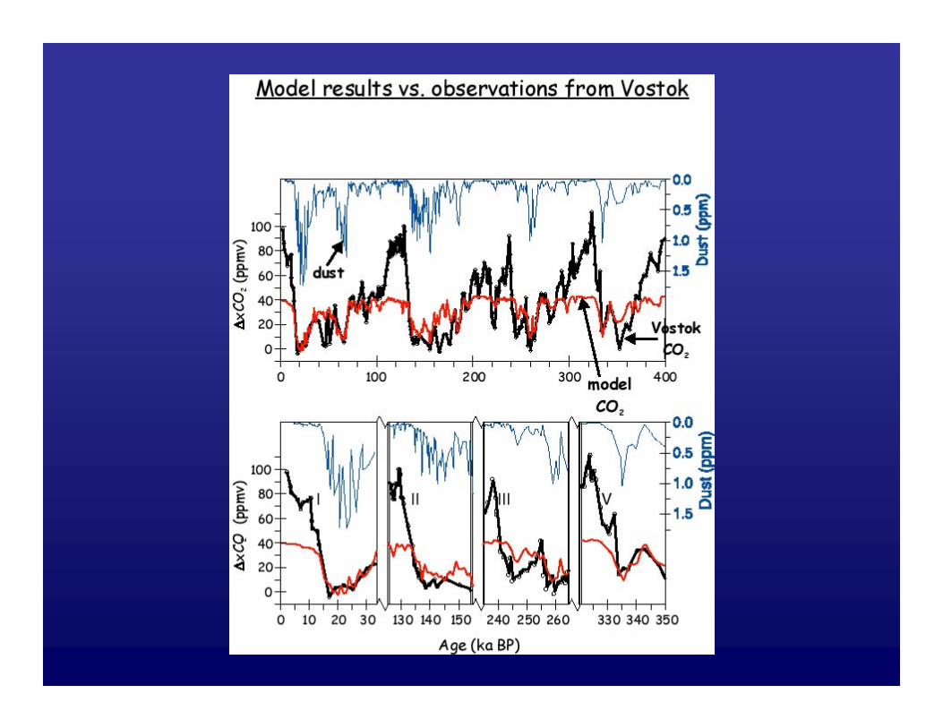
Implications for climate change• On time scales 102 - 105 years, natural concentrations of

atmospheric CO2 are largely set by CO2 balance at the ocean surface, particularly the Southern Ocean.

• There was also considerably greater supply of iron to the surface ocean as atmospheric dust.

• In glacial times the atmosphere contained substantially less CO2 than in interglacials.

• The timing and magnitude of changes in dust supply is consistent with their being the cause of a substantial part of the glacial-interglacial change in CO2

Source: N. Mahowald et al.,JGR 104,15895-15916 (1999)

Mahowald et al. Modelled dust deposition (g m-2 yr-1)Last Glacial Maximum

remineralization

gasexchange

scavenging

ocean

inter

aeoliandustdeposition

temperature + insolation

dissolution

sedimentarydiagenesis

dissolution

sedimentation

non-diatomproductivity

sediments

surfaceocean

continental

run-off

burial

e

KEY:CaCO3 C dustSiPO4Fe

diatomproductivity

Model biogeochemistry(Ridgwell, 2001)

Conclusions• In the HNLC regions of the open ocean, addition of iron

stimulates diatom blooms.

• There is depletion of inorganic nutrients and dissolved CO2 in the surface.

• The ecosystem is transformed from a low-particulate-export to a high export system.

• Models of the global marine /atmospheric carbon cycle suggest this effect is probably important in helping to explain the causes of glacial-interglacial atmospheric CO2 change.

• But the same models show that deliberate iron fertilization cannot “solve” the anthropogenic greenhouse effect.

• Realistically, it may be possible to sequester a few percent of the CO2 humans are emitting b y this method.

Fe induces decrease in silicon to carbon uptake ratio for the

ecosystem.• Measurements were made using 32Si uptake from

samples at 5m in and out of the patch, and 14C measurements made throughout the mixed layer. To obtain whole-mixed layer values, silicon uptake rates were assumed to be invariant through the mixed layer.

• Mean mixed layer Si:C = 0.18 ± 0.1 (n=11) in patch =0.36 ± 0.015 (n=2) out of

patch.Observations are in-situ confirmation of incubator

results (i.e. Hutchins and Bruland, 1998, Takeda, 1998) of effect of Fe on Si:C

1) Brief overview of history of iron limitation2) The HNLC areas – The Southern Ocean as

a key region for atmospheric CO2. (no time to explain!?)

3) Ironex II and SOIREE4) Why diatoms like iron5) Conclusions

1) Geo-engineering2) Glacial-interglacial effects.

21

0.50.25

PO4 uM:

Phosphate concentrations in surface water