carbon isotope measurements of surface seawater …ams/text bodies/hinger_et_al_2010... · carbon...

RADIOCARBON, Vol 52, Nr 1, 2010, p 69–89 © 2010 by the Arizona Board of Regents on behalf of the University of Arizona

69

CARBON ISOTOPE MEASUREMENTS OF SURFACE SEAWATER FROM A TIME-SERIES SITE OFF SOUTHERN CALIFORNIA

Elise N Hinger1 • Guaciara M Santos • Ellen R M Druffel • Sheila GriffinEarth System Science, Keck Carbon Cycle AMS Laboratory, University of California, Irvine, California 92697-3100, USA.

ABSTRACT. We report carbon isotope abundances of dissolved inorganic carbon (DIC) in surface seawater collected froma time-series site off the Newport Beach Pier in Orange County, California. These data represent the first time series of 14Cdata for a coastal southern California site. From a suite of samples collected daily from 16 October to 11 November 2004,14C values averaged 32.1 ± 4.4‰. Freshwater input from the Santa Ana River to our site caused 14C and 13C values todecrease. Since this initial set of measurements, a time-series site has been maintained from November 2004 to the present.Surface seawater has been collected bimonthly and analyzed for 14C, 13C, salinity, and CO2 concentrations. Water sam-ples from the Santa Ana River were collected during the wet season. California sea mussels and barnacle shells, ranging from4 to 6 months old, were also collected and analyzed. Results from May 2005 to January 2008 show no long-term changes in13C DIC values. 14C DIC values over the 2005–2006 period averaged 33.7‰; high 14C values were observed sporadically(every 6–7 months), suggesting the presence of open water eddies at our site. Finally, in 2007, a stronger upwelling signal wasapparent as indicated by correlations between 14C, salinity, and the Bakun index, suggesting that the 14C record is an indi-cator of upwelling in the Southern California Bight.

INTRODUCTION

Dissolved inorganic carbon (DIC) is the largest pool of carbon in ocean water and is the precursorof organic matter produced by phytoplankton in the surface ocean. Interannual DIC 14C variabilityis primarily an indicator of ocean mixing, and is an indicator of upwelling in the open ocean (Ekmanpumping; Guilderson et al. 2006) and coastal regions (Robinson 1981). Stable carbon isotope (13C)measurements of surface seawater and mollusks have also been used as a tracer of upwelling (Kill-ingley and Berger 1979; Sheu et al. 1996).

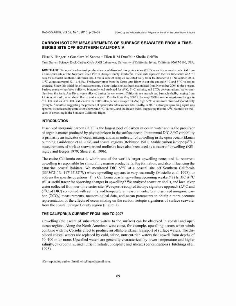
The entire California coast is within one of the world’s larger upwelling zones and its recurrentupwelling is responsible for stimulating marine productivity, fog formation, and also influencing theestuarine coastal habitats. We monitored DIC 14C at a coastal site off Southern California(333621N, 1175552W) where upwelling appears to vary seasonally (Masiello et al. 1998), toaddress the specific questions: 1) Is California coastal upwelling becoming weaker? 2) Is DIC 14Cstill a useful tracer for observing changes in upwelling? We analyzed seawater, shells, and local riverwater collected from our time-series site. We report a coupled isotope signature approach (14C and13C of DIC) combined with salinity and temperature measurements, total dissolved inorganic car-bon (CO2) measurements, meteorological data, and ocean parameters to obtain a more accuraterepresentation of the effects of ocean mixing on the carbon isotopic signatures of surface seawaterfrom the coastal Orange County region (Figure 1).

THE CALIFORNIA CURRENT FROM 1999 TO 2007

Upwelling (the ascent of subsurface waters to the surface) can be observed in coastal and openocean regions. Along the North American west coast, for example, upwelling occurs when windscombine with the Coriolis effect to produce an offshore Ekman transport of surface waters. The dis-placed coastal waters are replaced by cold, saline, nutrient-rich waters that upwell from depths of50–100 m or more. Upwelled waters are generally characterized by lower temperature and highersalinity, chlorophyll a, and nutrient (nitrate, phosphate and silicate) concentrations (Hutchings et al.1995).

1Corresponding author. Email: [email protected].

70 E N Hinger et al.

Over the past 50 yr, several programs have monitored the meteorology, oceanography, chemistry,and biology of the California Current System (CCS) from Oregon to Baja California. In these pro-grams, seasonal cruises reoccupy dozens of stations following grid lines from inshore to openwaters. Overviews of the recent state of the CCS are presented in the data reports published by theCalifornia Cooperative Oceanic Fisheries Investigations (www.calcofi.org) (Peterson et al. 2006;Goericke et al. 2007), the Climate Prediction Center (http://www.cpc.ncep.noaa.gov), and theNorthwest Fisheries Science Center (http://www.nwfsc.noaa.gov).

In general, the main observations provided by these programs along the North American west coast(36N to 57N) show that from 1999 to 2002, the CCS experienced strong summer upwelling and ashift to lower than normal sea surface temperatures (SSTs). During October 2002 to June 2005,weak El Niño conditions accompanied higher SSTs due to weak spring and summer upwelling southof Monterey Bay. In the Southern California Bight, SST anomalies were as high as 4 C above nor-mal (average seasonal temperature means from 1968–1996). In July to August 2005, upwelling ofcold, saline, nutrient-rich water returned to the Southern California coast and continued throughearly 2006 (Peterson et al. 2006). Upwelling was weak through June 2006 and above averagethrough fall (upwelling index anomalies were calculated relative to the 1948–1967 monthly means).In 2007, the CCS experienced near-to-above normal upwelling conditions from March to May andbelow average upwelling in June and July 2007 (Goericke et al. 2007). The cumulative upwellingfor 2007 was above average with a transition to higher upwelling (La Niña phase) in late 2007 toearly 2008 (http://www.cpc.ncep.noaa.gov).

Figure 1 Water collection station off Orange County in the Southern CaliforniaBight, USA (indicated by X). Bathymetry is indicated by lines of constant depth inmeters (after Bray et al. 1991).

Carbon Isotope Measurements of Surface Seawater from a Time-Series Site 71

THE SOUTHERN CALIFORNIA BIGHT

The Southern California Bight (SCB) extends from Point Conception south to Cabo Colnett, BajaCalifornia (575 km), with the California Current System (CCS) to the west. The CCS flows south-ward, between California’s shelf break to about 1000 km offshore. It is part of the clockwise geo-strophic flow of water in the North Pacific gyre, carrying relatively cold, fresh subarctic watersouthward. The eastward indentation of the Southern California coast results in a counterclockwisegyre, known as the Southern California Eddy, in which water from the CCS is carried inshore andnorthward through the center of the bight to form the Southern California Countercurrent (Figure 2).Also within the SCB is the California Undercurrent, a narrow northward-flowing current of tropicalorigin; it flows between 100 and 400 m depth along the continental slope (Tsuchiya 1975). While apoleward flow of water predominates in the SCB due to the Southern California Countercurrent (sur-face flow) and California Undercurrent (subsurface flow), there are seasonal variations in surfacewater currents. The poleward surface flow of the Southern California Countercurrent is strongestduring the summer months and continues through fall and winter. In spring, when equatorwardwinds along the southern California coast are strongest, the northward flow weakens or reverses,allowing an equatorward surface flow to prevail (Bray et al. 1991; PSCB 1990) (Figure 2).

The sea floor of the bight is characterized by a series of deep basins (610–2500 m deep), islands, andsubmerged seamounts. The numerous basins, narrow continental shelf, and steep slopes throughoutthe SCB region allow deep water to exist near shore (Bray et al. 1991; PSCB 1990).

The SCB and its mainland drainage basin experience a semi-arid Mediterranean climate. Monthlyprecipitation near our sampling site peaks during the winter months, with a 5-yr range of 30–80 mm,while summer months have near zero precipitation. Fall and spring months experience intermediatevalues of 0–40 mm/month (http://waterdata.usgs.gov). This combination of semi-arid climate andlow precipitation makes the rivers draining into the bight low flow.

Environmental changes in the SCB are linked to long-term, interannual patterns, such as El Niño-Southern Oscillation (ENSO), rather than to seasonal cycles (Bray et al. 1991). The surface waters

Figure 2 The average surface currents and salinity values in the Southern California Bight in (a) spring and (b) summer from1984–1995. Northward flow along the coast is strongest in the summer months and weakens or reverses in the spring, allow-ing equatorward surface flow to prevail. Length of arrows represents relative geostrophic velocity. Color indicates salinity and“X” indicates our NBP sampling site. High salinities along the coast are associated with upwelling (Bray et al. 1991).


in the SCB originate primarily from the CCS and are therefore more nutrient-rich, less saline, andcooler, except when periodic ENSO events occur (PSCB 1990). ENSO events cause cooler surfacewaters to be replaced with nutrient-poor, warmer waters and a deeper surface mixed layer. Changesin weather and alterations in the marine community composition of the SCB can also be observedduring ENSO events.

SAMPLING SITES

To determine a suitable sampling site for the coastal Orange County region in California, 4 seawatersamples were collected, processed, and measured (for DIC 14C, DIC 13C) from the shoreline, theNewport Beach Pier (NBP), and the Balboa Pier (BP) located 1.7 miles southeast of the NBP (Fig-ure 3). The preliminary results indicated that these sites have similar isotopic compositions, andbecause of logistical considerations, the NBP site was chosen as our sampling site.

The NBP site is located about 2 miles southeast of the mouth of the Santa Ana River. The Santa AnaRiver system is one of the largest rivers in Southern California with a watershed of ~2800 squaremiles (http://sawpa.org/about/watershed.htm). The river begins in the San Bernardino Mountains,travels through the Orange County Coastal Plain, and into the Pacific Ocean. Much of the Santa AnaRiver is a concrete-lined channel. It is characterized by near zero flow during the dry seasons andhigh surface flows through spring and early summer.

METHODOLOGY

Water Sample Collection

Surface seawater samples were collected daily from the NBP site from 16 October to 11 November2004. Following this initial collection series, samples were collected biweekly between 10:00 AM

Figure 3 Satellite photo of the coastal region of Orange County. From left to right: the Santa Ana Rivermouth (SAR), the Newport Beach Pier (NBP) and the Balboa Pier (BP) are marked. These are the 3 sitesfrom which samples were collected for this study (http://maps.google.com/).


and 1:00 PM (to assure the same tidal conditions). Surface waters were collected from a platform atthe end of the pier that was lowered down to the water for sampling. Water samples were collectedoccasionally from the Santa Ana River at the Hamilton overpass, located ~1.4 miles upriver of theSanta Ana River mouth (Figure 3).

Two types of collection bottles were used. Seawater and river water samples for DIC 14C and 13Canalyses were collected in 500-mL glass bottles with ground glass stoppers. Samples analyzed forCO2 and salinity were collected in 200-mL Kimex® bottles with plastic caps. On 20 September2007, the sampling bottles used for CO2 and salinity measurements were replaced with Pyrex® 250-mL laboratory bottles with polypropylene caps. The previous collection bottles were found to beinferior because of evaporation of water from the samples.

Several precautions were taken to avoid contamination. Bottles and stoppers were washed using adilute soap solution and water, followed by a 10% HCl solution and distilled water. The glasswarewas baked at 550 C for 2 hr and stored in plastic bags.

Four samples were collected during each sampling: 2 for 14C analysis, 1 for CO2, and 1 for salin-ity. At the sampling site, a 10-L bucket, equipped with a long piece of silicone tubing, was loweredinto the water and rinsed several times prior to sampling. Each sample bottle was then filled with thetubing placed at the bottom of each bottle and allowed to overflow twice its volume. After all watersamples were collected, the 14C and CO2 samples were poisoned with 100 L and 50 L of sat-urated HgCl2 solution, respectively. The glass stoppers were coated with Apiezon N grease using asyringe to ensure a gas-tight seal. Each stopper was secured with 2 wide rubber bands placed aroundthe cap and base of the bottle. After water collection, a thermometer (with an accuracy of ±1 C) wasplaced in the remaining water and temperature was recorded along with other meteorological data,e.g. wind speed and direction, air temperature, recent precipitation events and possible river dis-charges, and water temperature measurements made by the lifeguards.

Calcium Carbonate Collection

Live California sea mussels (Mytilus californianus) and barnacle shells (spp. unknown) were col-lected from a support post of the pier, next to the water sampling site. These 2 species were selecteddue to their abundance in Southern California and availability at our sampling station. The first col-lection was performed on 4 May 2006 and the age of the mussel was estimated to be ~6 months oldfrom its shell length of ~35 mm (Coe and Fox 1942). A second mussel shell was collected on 18June 2007 and its age was similarly ~6 months. On 31 January 2008, a third and fourth mussel werecollected and estimated to be ~5 and ~4 months old, respectively.

CO2 Extraction

Water samples for 14C and 13C analyses undergo CO2 extraction in the laboratory using a dedi-cated vacuum line. While 2 full bottles are collected for 14C analysis, only one-half bottle (~250 mL)is needed per sample. This allows us to make up to 4 measurements of the same water to assess accu-racy, if necessary.

The samples were stripped of CO2 using a modified extraction procedure of published protocols(McNichol and Jones 1991; McNichol et al. 1994). Half of the water in a DIC collection bottle wastransferred into a custom reaction apparatus in a high-purity N2 glove bag. The original bottle thatcontained the rest of the water sample was resealed, reweighed, and stored for later use. The sampleis connected to the vacuum line where it is acidified with 3 mL of 85% phosphoric acid and recircu-lated in the line with clean N2 for 10 min. Two dry ice-isopropanol slush traps collect water and a


liquid nitrogen trap collects CO2. The CO2 is cryogenically purified and transferred to a calibratedvolume for a pressure measurement, enabling us to determine the CO2 of the sample.

The CO2 sample was split into 3 aliquots and flame-sealed into Pyrex tubes. Approximately 1.75mL of CO2 gas was used to produce ~1 mg C graphite for the 14C measurement, 0.54 mL for 13Canalysis, and the excess gas was archived.

Organic matter on the shell samples was separated from the calcite shell via microwaving andremoval with a spatula. Dry, crushed calcium carbonate samples were placed in 3-mL Vacutainer®

vials (disposable blood sample vials), leached using 2 mL 0.1N HCl to remove 50% of the sample’ssurface mass, and rinsed with deionized water. Vacutainers were then evacuated through the rubberstopper using a hypodermic needle connected to a vacuum line. Following evacuation, 0.8 mL ofphosphoric acid was injected into each Vacutainer using a gas-tight syringe and hydrolyzed for 25min at 70C to generate CO2 (Santos et al. 2004).

Graphite Sample Production

Carbon dioxide samples were converted to graphite by reduction with H2 in the presence of an ironpowder catalyst at 550 C. Mg(ClO4)2 is present during the reaction for water removal (Santos et al.2004, 2007). Following graphitization, samples are pressed into aluminum target holders that aremounted into the ion-source wheel and measured in the AMS system.

14C and 13C Measurements

All 14C and 13C results (including freshwater and carbonate samples) obtained during this studyare listed in Tables 1 and 2. 14C results were obtained at the KCCAMS/UCI facility, which isequipped with a compact AMS particle accelerator from National Electrostatics Corporation (NEC0.5MV 1.5SDH-2 AMS system) dedicated to measuring 14C. This compact system measures all 3carbon isotopes (14C, 13C, and 12C), allowing us to produce high-precision measurements (Santos etal. 2007). Each sample is corrected for fractionation using its own AMS 13C value (which can dif-fer by several per mil from the 13C of the original material, if fractionation occurs during the AMSmeasurement). From general carbonaceous samples measured by this AMS system since 2002, theoverall fractional scatter from the primary standard oxalic acid I (OX-I), as well as the accuracybased on the measurement of multiple secondary standards (OX-II, FIRI-C, FIRI-D, for example)has been ~3‰ (±1 ) (Santos et al. 2007).

Table 1 Complete DIC 14C, 13C, temperature, salinity, and CO2 values from surface seawatersamples collected from sites off the coast of Southern California. Calcium carbonate results aremarked with asterisks. One result is from a freshwater sample from the Santa Ana River. The 14Cresults are reported as age-corrected 14C (‰), as defined by Stuiver and Polach (1977). Total dis-solved inorganic CO2 results were calculated from the manometric measurement of CO2 after acid-ification of seawater. Uncertainty for CO2 values is ±40 mol/kg.

Sample ID(dates in month/day/year)

Tempa

(C)Salinity (‰)

Lab nr(UCIAMS)

14C(‰) ±

13C(‰)b

CO2

(mol/kg)

8/20/2004 Near NBP - shorec 10407 37.8 2.9 — —10408 32.8 2.4 1.6 196510409 33.1 2.8 — 195910410 35.7 2.9 1.6 1953

8/20/2004 NBP Pierc 10412 31.1 2.8 1.8 194810413 35.2 2.9 1.7 193810414 32.0 2.4 1.8 1937


9/22/2004 Balboa Pierc 13359 29.7 1.6 1.9 210113367 29.2 1.9 1.8 195113361 27.1 1.5 1.8 1946

9/22/2004 NBP Pierc 13358 32.7 1.9 1.7 198013360 31.9 1.7 1.7 195113362 32.2 1.7 1.8 1975

10/16/2004 19.8 33.34 13370 25.8 1.5 1.8 199510/17/2004 20.2 30.86 13371 37.8 1.5 1.3 190710/18/2004 20.0 33.24 13356 35.2 1.7 1.6 1954

13357 32.9 1.6 — —13372 33.9 1.5 1.7 2012

10/19/2004 18.8 33.12 13373 35.5 1.5 1.7 201910/20/2004 19.6 33.17 13374 34.9 1.8 1.9 197410/21/2004 20.5 33.06 13375 37.7 1.5 1.5 1976

17053 31.6 1.7 1.5 200310/22/2004 19.4 32.87 13376 32.5 1.5 1.7 160710/23/2004 21.2 29.98 13377 32.3 1.6 0.1 192910/24/2004 22.1 28.40 13378 20.9 1.7 0.5 2008

17054 23.6 1.5 1.1 202910/25/2004 24.0 28.89 13368 28.3 1.6 0.0 195910/26/2004 18.1 31.44 13380 32.4 1.6 1.6 193410/27/2004 19.5 32.87 13381 34.6 1.5 1.8 196910/28/2004 19.8 33.12 13382 31.0 2.0 1.7 196110/29/2004 20.0 33.05 13383 36.4 1.5 1.6 198610/30/2004 21.5 33.16 13384 26.8 1.6 1.5 1805

17055 29.9 1.6 1.5 199610/31/2004 20.5 33.06 13385 34.8 1.7 1.6 198811/1/2004 19.5 33.15 13386 33.3 1.6 1.4 200511/2/2004 19.5 33.17 13363 26.8 1.7 1.6 1987

17056 31.7 1.6 1.6 200211/3/2004 19.5 33.18 13364 33.0 1.5 1.8 196411/4/2004 19.4 33.08 13365 30.0 1.6 1.2 19461/15/2005 16.5 24.45 17057 21.0 1.5 2.1 1967

17058 22.7 2.5 1.9 19192/9/2005 15.8 33.10 17059 32.0 1.5 1.3 19922/12/2005 16.2 32.75;

32.85d17060 34.4 1.9 1.5 1993

17061 31.6 1.5 1.5 19872/23/2005 16.8 31.86 17063 38.9 1.5 1.2 1976

17064 33.9 1.6 1.1 197622427 32.1 1.7 — —23542 38.7 1.5 1.1 1990

Table 1 Complete DIC 14C, 13C, temperature, salinity, and CO2 values from surface seawatersamples collected from sites off the coast of Southern California. Calcium carbonate results aremarked with asterisks. One result is from a freshwater sample from the Santa Ana River. The 14Cresults are reported as age-corrected 14C (‰), as defined by Stuiver and Polach (1977). Total dis-solved inorganic CO2 results were calculated from the manometric measurement of CO2 after acid-ification of seawater. Uncertainty for CO2 values is ±40 mol/kg. (Continued)


Tempa

(C)Salinity (‰)

Lab nr(UCIAMS)

14C(‰) ±

13C(‰)b

CO2

(mol/kg)


3/11/2005 17.5 32.54 17065 32.5 1.7 1.5 198517066 33.4 1.7 1.4 1980

3/25/2005 17.0 32.59 17068 32.5 1.7 0.8 197722428 32.1 1.8 — —23543 34.8 1.6 0.6 2065

3/25/2005 SAR — 0.36 17070 1.5 1.5 11.3 296017071 0.3 1.7 11.3 2963

4/15/2005 17.0 32.44 17073 64.6 1.7 1.3 196017074 64.8 1.8 — —17075 65.9 1.8 1.3 196517076 66.3 2.4 1.4 1938

5/9/2005 19.8 33.01 17077 40.1 1.8 1.5 198817079 33.6 1.7 1.4 196922430 32.6 1.5 — —

5/27/2005 19.5 33.44 17080 30.0 1.7 1.9 195922431 30.0 1.4 — —23544 33.3 1.7 2.0 1970

6/13/2005 22.0 33.34 17082 34.8 1.6 2.6 182222433 31.8 1.5 — —23545 30.4 1.7 2.1 —

6/27/2005 19.5 33.41 22434 39.4 1.5 1.8 196222435 43.7 1.7 3.0 196323546 44.3 1.5 1.3 187823548 45.7 1.5 — 2003

7/7/2005 21.5 33.49; 33.48d

22437 36.9 1.7 2.9 1803

22438 35.9 1.5 2.8 18127/21/2005 24.5 33.45 22439 30.7 1.6 — 1828

22440 30.7 1.5 2.8 18397/21/2005 SAR 32.76 22441 42.2 1.6 1.8 25668/4/2005 21.5 33.32 22442 20.1 1.5 3.0 1789

22443 29.3 1.8 3.6 174323549 32.0 1.5 3.1 —23550 32.6 1.6 — 1772

8/18/2005 21.0 33.32 22444 29.6 2.5 2.7 184723551 31.0 1.6 — —

9/1/2005 23.0 33.27 22446 29.9 1.9 2.4 191122447 31.5 1.5 2.6 1897

9/19/2005 20.5 33.31 22448 39.2 1.5 2.6 186022449 38.8 1.5 2.4 1892

10/7/2005 19.2 33.33 22450 35.0 1.7 — 193722451 32.0 1.6 2.0 1804



Tempa

(C)Salinity (‰)

Lab nr(UCIAMS)

14C(‰) ±

13C(‰)b

CO2

(mol/kg)


22452 31.6 1.6 — —22453 36.3 1.8 2.0 1950

10/21/2005 19.0 33.25 23552 31.7 1.5 — 191623553 35.8 1.4 2.0 1936

11/4/2005 19.0 33.30 22454 33.7 1.7 2.1 190523554 26.9 1.8 1.4 2167

11/18/2005 18.5 33.29 23555 31.1 1.5 1.7 194212/2/2005 16.5 33.29 23556 36.1 1.6 1.6 1962

31143 37.3 1.4 1.6 197412/16/2005 15.5 33.39 23557 33.5 1.4 1.2 202312/29/2005 17.5 33.27 23558 36.6 1.4 1.4 1997

31144 33.5 1.4 1.3 19681/13/2006 16.3 33.24 23559 49.9 2.0 1.5 1951

31145 52.2 1.4 1.6 19472/2/2006 15.5 33.40 23561 41.7 1.7 1.7 19612/16/2006 14.0 33.42 23560 41.1 1.5 3.3 19663/2/2006 17.0 33.22 23562 34.3 1.5 1.7 19683/20/2006 13.0 33.40 43656 25.8 1.3 0.8 20394/6/2006 15.0 30.34 31146 28.1 1.3 0.8 2064

31147 29.7 1.3 0.7 208731148 27.5 1.3 — 2075

4/20/2006 17.0 33.43 31149 27.8 1.6 1.3 19425/4/2006 18.5 32.82 31150 27.3 1.4 1.3 1948

43657 26.2 1.3 1.2 19075/4/2006 Mussel Shell* 31151 34.8 1.3 — —5/4/2006 Barnacle Shell* 31152 36.3 1.3 — —5/18/2006 18.0 33.50 31153 24.9 1.3 1.6 19546/1/2006 18.5 33.45 31154 27.8 1.3 2.2 19006/15/2006 18.0 33.42 31155 34.3 1.9 1.5 1986

31156 31.1 1.3 1.3 20097/1/2006 17.0 33.46 31157 37.7 1.4 1.2 20147/15/2006 19.5 33.43 31158 31.3 1.3 1.6 19957/29/2006 25.0 33.52 31159 28.9 1.3 1.9 1963

43658 31.3 1.8 2.0 18948/15/2006 20.0 33.40 31160 45.0 1.6 1.9 1969

43659 47.1 1.5 1.8 1975— — — 1.9 —

8/29/2006 19.0 33.44 31161 33.0 1.4 1.6 19839/14/2006 19.0 33.41 31162 32.2 1.4 1.6 20229/28/2006 18.5 33.40 31163 30.9 1.4 1.5 199010/17/2006 19.0 33.39 31164 33.7 1.4 1.6 197611/8/2006 19.0 33.34 31165 32.9 1.4 1.7 1959



Tempa

(C)Salinity (‰)

Lab nr(UCIAMS)

14C(‰) ±

13C(‰)b

CO2

(mol/kg)


11/22/2006 19.0 33.35 — — — — —12/28/2006 14.5 33.03 43660 32.1 1.4 1.5 20361/11/2007 14.0 33.54 43661 33.7 1.3 1.2 19711/11/2007 SAR/ocean mixture — 24.81 43662 12.2 1.3 4.8 27341/26/2007 15.0 33.58 43663 36.7 1.4 1.3 19732/14/2007 15.0 33.40 43664 48.4 1.3 0.7 20103/17/2007 14.5 33.60 43665 29.9 1.7 1.4 19214/2/2007 15.0 43666 27.6 1.3 1.0 1969

45399 27.7 2.1 — —4/18/2007 15.0 33.67 43667 26.4 1.3 1.2 1952

45400 27.8 2.5 — —5/3/2007 17.0 43668 22.1 1.3 1.1 20205/18/2007 15.5 33.76 43669 20.9 1.3 2.1 18845/31/2007 17.0 33.79 43670 22.7 1.3 2.1 18246/18/2007 18.0 33.75 43671 25.3 1.6 1.3 19956/18/2007 Mussel Shell* 43681 36.4 1.5 — —

45410 32.3 2.3 — —7/5/2007 22.0 33.74 43672 25.7 1.3 1.8 19267/20/2007 20.0 — 43673 26.2 1.3 1.6 19268/6/2007 23.0 — 43674 23.1 1.3 2.1 19008/21/2007 22.0 33.69,

33.69d43675 27.1 1.3 2.0 1918

9/6/2007 20.5 33.64 43676 28.9 1.6 1.7 19469/20/2007 19.0 33.63 43677 27.6 1.3 1.6 197910/5/2007 18.0 33.53 43678 29.6 1.3 1.5 192110/19/2007 17.0 33.45 43679 30.4 1.3 1.5 194311/6/2007 17.0 33.52,

33.52d43680 27.0 1.3 1.8 1913

11/20/2007 15.5 33.55 45401 29.6 2.1 1.6 195212/6/2007 16.0 33.44 45402 25.0 2.2 1.3 195112/28/2007 13.0 33.39 45403 29.5 2.2 1.4 19741/4/2008 14.0 33.43 45404 29.1 2.1 1.4 19891/31/2008 14.0 33.42,

33.42d45405 31.2 2.3 1.5 1974

1/31/2008 Mussel Shell A* 45411 29.1 2.2 — —1/31/2008 Mussel Shell B* 45412 27.4 2.2 — —

aTemperature measured from the remaining water mass after sampling.b13C values measured using continuous-flow stable isotope ratio mass spectrometer (Finnigan Delta-Plus CFIRMS).cPreliminary 14C measurements to help on the selection of the sampling station.dDuplicate measurements performed on the same water mass to evaluate procedural error.



Tempa

(C)Salinity (‰)

Lab nr(UCIAMS)

14C(‰) ±

13C(‰)b

CO2

(mol/kg)


To obtain high-precision measurements on wheels composed of DIC samples, we added to the usualsets of 6–8 OX-I primary standards: OX-II samples, 2 to 3 DIC procedural blanks, and secondarycoral standards produced in the same fashion as unknown samples (Table 2). Individual targets werecycled at least 12 times, and analyzed for 50,000 14C events. The individual statistical error barsfrom these samples were typically ±2‰ (±1 ) (Tables 1 and 2). These errors were calculated basedon counting statistics and scatter in multiple measurements of each sample, along with propagateduncertainties from normalization to standards, background subtraction, and isotopic fractionationcorrections, as mentioned above.

For proper DIC 14C background corrections, we measured the mass and the 14C AMS signatureof several procedural blank samples (Table 2). To produce these samples, ~60 mg of spar calcitecrystals (a 14C-free material with initial 14C value of 1000‰) were dissolved into a previouslystripped seawater sample (and therefore free of DIC) in the presence of a high-purity N2 environ-ment. In this case, the 14C result obtained from the procedural blank represents the amount of mod-ern carbon added to the sample during CO2 stripping, graphitization, and pressing of graphite sam-ples. The 14C AMS results from the DIC procedural blank averaged 993.6‰ (equivalent to Fm =0.0065; Table 2). This result constitutes a modern carbon contamination of <0.8% of the sample, andwas subtracted from the final DIC 14C results listed in Table 1.

Stable isotope DIC13C measurements were made using a continuous-flow isotope ratio mass spec-trometer (Delta-Plus CFIRMS), interfaced with a Gasbench II and dual inlet (for CO2 analysis). Forstandard control, the precision of the equipment was also evaluated by sets of CO2 gas from OX-Icombustion produced and measured at the same time as unknown samples. The standard deviationof these measurements was 0.09‰ (n 32, not shown in Table 2).

To verify the experimental error associated with the DIC sample procedure, we analyzed multiplesamples from the same sampling date (Table 1), in addition to the DIC blanks and coral standard

Table 2 Complete DIC 14C and 13C values from blanks and secondary standards used to back-ground-correct and evaluate precision and accuracy of the results produced. Calcium carbonateblank and secondary standard are marked with asterisks. In addition, batches of CO2 DIC samplesto be measured by the stable isotope ratio mass spectrometer were also followed by CO2 aliquots ofOX-I (oxalic acid I) produced from a large amount of gas to verify the procedural error of thisinstrument (results not shown). The standard deviation of these measurements was 0.09‰ and stan-dard error was 0.02‰ (n32).

nFma

average

aFraction modern of carbon (Stuiver and Polach 1977).

Fmst. error

14C (‰)b

average

b14C values expressed as 14C, (Stuiver and Polach 1977)

14C (‰)st. error

13Caveragec

c13C values measured using continuous-flow stable isotope ratio mass spectrometer (Finnigan Delta-Plus CFIRMS).

13Cst. errord

dProcedural error based on number of replicates.

DIC CSTDe

eDissolved coral standard produced in previously stripped seawater samples.

21 0.9440 0.0004 62.0 0.35 0.57 0.013DIC Calcitef

fDissolved mineral calcite produced in previously stripped seawater samples to determinate procedural background.

12 0.0065 0.0008 993.6 0.75 1.60 0.025Calciteg*

gSolid mineral calcite.

4 0.0017 0.0003 998.3 0.27 — —FIRI-Ch*

hFIRI-C marine turbidite, consensus value of 18,176 yr BP (Scott et al. 2004).

4 0.1036 0.0002 897.3 0.18 — —


samples (Table 2). In terms of reproducibility, the DIC 14C measurements are within the stated pre-cision of ±2.0‰ (±1 ), based on a pooled standard deviation calculation (McNaught and Wilkinson1997) of the 39 sets of replicated measurements (Tables 1 and 2). The results obtained for DIC 13Cthrough CFIRMS measurements yielded a pooled standard deviation of ±0.2‰ (±1 ; 38 datapoints). Since the nominal or statistical propagated errors from individual measurements (as shownon Tables 1 and 2) are mostly smaller than these calculated experimental uncertainties, we have cho-sen to use the larger errors during our discussion.

Calcium carbonate samples measured with the AMS system were background-corrected with theproper blank and checked by secondary standard samples (calcite crystals and FIRI-C marine tur-bidite, respectively) and their results are shown in Tables 1 and 2 (marked with asterisks).

Temperature, Salinity, and CO2

Temperature, salinity, and CO2 values from surface seawater are shown on Table 1. Temperaturemeasurements were taken in situ. The temperature values obtained were later compared with thevalues obtained by the Newport Beach lifeguards from the same station as well as a Southern Cali-fornia Coastal Ocean Observing System (http://www.sccoos.org) automated station off Balboa Pier(Figure 4). The measurements made by the Newport Beach lifeguards are performed daily usinga thermometer (with accuracy of ±0.1 F) placed at ~3 m depth (from mean tide level) below thesurface water. Temperature measurements obtained using these 3 methods show slight differences,but show the same general trend. Our temperature measurements are made in the upper 1 m, whilethe other 2 measurements are made at 3 m depth. All temperature values used in the Discussion andResults section are our measurements.

Salinity measurements of seawater were made by the Scripps Oceanographic Data Facility (http://sts.ucsd.edu/sts/chem) using a Guildline Autosal 8400A salinometer (nominal accuracy of0.002‰). To determine measurement precision, 1 unknown sample per group submitted was

Figure 4 Temperature results obtained by 3 distinct proxies: (�) from NBP at ~3 m depth, depending on the tidal conditions,recorded by the lifeguards; () from the NBP in surface seawater samples collected in this work; and (�) from Balboa Pier at~3 m depth obtained by the Southern California Coastal Observation System (SCCOOS) database (http://www.sccoos.org/).

14

16

18

20

22

24

26

Tem

pera

ture

(oC

)

10

12

14

16

18

20

22

24

26

Jan-05 Jul-05 Jan-06 Jul-06 Jan-07 Jul-07 Jan-08

Tem

pera

ture

(oC

)


selected to be remeasured, yielding a standard error calculation of 0.04‰ (±1 ), based on 5 pairs(Table 1).

CO2 values were calculated from the manometric measurement of CO2 after the acidification ofseawater. Initially, the CO2 manometric calculation assumed a room temperature of 20C (itali-cized values in Table 1). Beginning with samples from December 2006, actual room temperaturewas recorded during the CO2 extraction of each water sample. The recorded temperature was takeninto account for the CO2 manometric calculation resulting in a more accurate value. The maximumerror for these measurements is approximately ±40 mol/kg.

RESULTS AND DISCUSSION

NBP Daily Collection (October–November 2004)

Figures 5a–f show data obtained from temperature, salinity, CO2, DIC 14C, and 13C measure-ments from the NBP site, as well as Santa Ana River discharge data (obtained from the US Geolog-ical Survey database) from 10/15/04 to 11/11/04. The lines in Figures 5c–e represent the 3-pointmoving average. This experiment was designed to determine the daily variability of the carbon iso-topic ratios and other chemical and meteorological parameters at this coastal site.

The SST values averaged 20.0 C with higher values (up to 24.0 C) from 10/23/04–10/25/04 (Fig-ure 5a). Salinity values averaged 33.16‰, with lower values (28.40–32.87‰) in samples collectedon 10/17/04 and 10/23/04–10/26/04 due to admixture with Santa Ana River water (Figure 5b,f).CO2 values averaged 1975 µmol/kg and showed no significant trend (Figure 5c). The 14C valuesranged from 20.9‰ to 37.8‰, with an average value of 32.1‰ (Figure 5d). The 13C values rangedfrom –1.1‰ to +1.9‰ with an average value of 1.6‰ and a distinct low from 10/23/04–10/25/04(Figure 5e).

Three precipitation events occurred during the NBP Daily Collection series (Figure 5f). On 10/17/04, a rain event (12 mm) resulted in a decreased salinity of 30.86‰ at our site. On 10/20/04, a sec-ond rain event (50 mm) resulted in high Santa Ana River discharge from 10/20/04–10/25/04 andsalinity values as low as 28.40‰ at our site. A third rain event occurred on 10/26/04–10/27/04 (31mm), resulting in high Santa Ana River runoff from 10/27/04–10/30/04. However, the salinity at oursite remained constant at 33.10‰ during this period, indicating that the runoff from the third eventdid not reach our sampling site.

Analysis of wind patterns (not shown in Figure 5) during this period explains the lack of a thirdlower salinity signal. Typical winds at our site are of southwest origin (perpendicular to our NW-SErunning coast) that strengthen in the afternoon and weaken in the evening. However, there werestrong southerly winds (10–20 mph) on 10/26/04 and then easterly winds (10–15 mph) on 10/27/04.These atypical winds coincided with the third rain event and most likely pushed Santa Ana Riverwater towards the northwest, away from our collection site. During typical conditions (that occurredthroughout the rest of October 2004), winds from the southwest would decrease the off-coast move-ment of Santa Ana River runoff, causing the freshwater to spread along the coastline.

Freshwater input from the Santa Ana River also appears to have caused lower than average DIC14C and 13C values along with increased SST. When local river input is not present, salinity aver-aged 33.14‰. We found that salinity measurements were essential to detect the presence of fresh-water at our site.


Santa Ana River Input to the NBP Site

As mentioned earlier, the Santa Ana River system is one of the largest rivers in Southern California,and its mouth is located about 2 miles northeast of our sampling site (Figure 1). Since we observedadmixture of freshwater at our site during the end of 2004, we decided to sample river waters tomake isotopic measurements as well. Water samples were collected occasionally from upriver.

Figure 5 NBP Daily Collection (a) SST, (b) salinity, (c) CO2, (d) 14C,(e) 13C and (f) Santa Ana River discharge from 16 October to 11 Novem-ber 2004. Trend lines for 14C, 13C, and CO2 are 3-point moving aver-age determinations.


CO2 measured in 3 samples of Santa Ana River water (2960, 2566, 2734 mol/kg on 3/25/05, 7/21/05, 1/11/07, respectively—denoted by SAR in first column of Table 1) were higher than in sea-water. The salinity values of the SAR samples are 0.36‰, 32.77‰, and 24.81‰, respectively, indi-cating that the SAR channel acts as a reverse estuary, changing direction of water flow seasonally.

14C results of the SAR samples are 0.8‰ (average of 2 points), 42.2‰, and 12.2‰, on 3/25/05,7/21/05, 1/11/07, respectively, when 13C results are –11.3‰, 1.8‰, and –4.8‰. These values cor-roborate the presence of seawater in the channel. The low carbon isotopic results suggest that theSanta Ana River can also be a source of low isotopic values to the NBP site. The 13C value from 3/25/05 (11.3‰) is likely a result of remineralization of organic matter that contains low 13C values.Since the beginning of summer 2005 to January 2008, there was little to no precipitation and no sig-nificant input of water from the Santa Ana River observed at the NBP site. However, the variabilityof these 3 proxies (DIC 14C, DIC 13C, and salinity) for the few samples measured are in goodagreement, and suggests mixing of Santa Ana River water with near-shore ocean water predictablyalters the isotopic and salinity signals at the NBP site.

NBP Long-Term Collection

We present water temperature, CO2, DIC 13C, DIC 14C, and salinity values, and the Bakun index(Bakun 1973, from 33N, 119W), from 5/05 to 1/08 in Figures 6a–f. The trend lines represent the3-point moving averages. While data for all samples are listed in Table 1, only data from sampleswith salinity values 33.00‰ are shown in Figures 6a–f to ensure that the comparisons among theseproxies are from marine origin only (i.e. data from 4/6/06, 5/4/06, and 1/11/07 are not plotted in Fig-ure 6). While some 14C and 13C values between January and May 2005 are not depleted, high pre-cipitation and runoff from the Santa Ana River continued to reach the NBP site during this period,resulting in salinity values consistently lower than 33.00‰ (24.45–32.85‰). To maintain consis-tency, data from the period prior to May 2005 is not included in Figure 6.

The SST values ranged from 13–25 C and averaged 18 C over the 3-yr period. Maximum SST val-ues were reached in 7/05, 7/06, and 8/07 with values of 24 C, 25 C, and 23 C, respectively. SSTminima occurred in 3/06, 1/07, and 12/07 with values of 13 C, 14 C, and 13 C, respectively (Figure6a). Total CO2 values averaged 1947 mol/kg with no significant trend overall, though a minimumin CO2 (1743 µmol/kg) occurred in 8/05 (Figure 6b). A small decrease in 13C DIC values isobserved from 2005–2008 (~0.5‰); values averaged 1.6‰. The sample from 2/16/06 had a notice-ably high value of 3.3‰, while samples from 4/6/06 (3 replicates) were noticeably low (0.6‰)(Figure 6c).

No long-term change in DIC 14C values is observed over the 2005–2006 time series and valuesaveraged 33.7‰. High 14C values were found for 4/15/05 (see Table 1), 6/27/05, 1/13/06, 8/15/06,and 2/14/07 (65.4‰, 43.3‰, 51.0‰, 46.0‰, and 48.4‰, respectively). In 5/07, DIC 14C valuesreached a minimum of 20.9‰ (Figure 6d), then increased slightly to 1/08.

Salinity values remained somewhat constant through 11/06, averaging 33.37‰. Salinity valuessteadily increased to 33.80‰ by 5/07 and then decreased to 33.42‰ by 1/08 (Figure 6e).

The 14C values of shell samples collected from the NBP site on 05/04/06 (~6-month-old musseland barnacle shells), 1/18/07 (~6-month-old mussel), and 1/31/08 (~4- and ~5-month-old mussels)yielded 34.8‰, 36.3‰, 32.3‰, 29.1‰, and 27.4‰, respectively (asterisks in Table 1). Theseresults are within the ranges of the DIC 14C values obtained for their individual estimated ages.


Figure 6 NBP Long Term Collection (a) SST, (b) CO2, (c) 13C, (d) 14C, (e) salinity measurements of seawater sam-ples from this work, and (f) Bakun index values (Bakun 1973) for 33N, 119W from 2005 to 2008. Trend lines are 3-point moving average determinations. Results from samples with salinity values <33.00‰ were removed to assure thatthe comparisons among proxies are from marine environmental samples only. The entire data set with all measurementsand determinations obtained for this work is in Table 1.


Killingley and Berger (1979) reported a record of seasonal upwelling from the stable carbon isotopemeasurements of modern mollusks shells that showed lower 13C values from upwelled wateradvecting from depth (Kroopnick et al. 1970). Our DIC 13C values show a significant anticorrela-tion with the CO2 measurements (r 0.79) (Table 3). On 4/6/06, a very low DIC 13C value wasobtained (0.75‰, n2, Table 1). This low 13C value is coincident with a maximum CO2 value(2075 M/kg, n3) that may have been caused by decomposition of 13C-depleted organic material(Sheu et al. 1996). However, because numerous factors affect DIC 13C values and CO2 concen-trations, we cannot definitively assign a cause or causes to this correlation.

High 14C values occurred every 6–7 months from 6/05 through 2/07 (Figure 6d). Using satellitedata, DiGiacomo and Holt (2001) determined that small-scale eddies (<50 km diameter) frequentlyoccur in the SCB during winter, including a cluster of eddies near the southern coast of San Clem-ente Island and around Catalina Island (~45 km from the NBP). Throughout the rest of the year,eddies are distributed throughout the SCB but in fewer numbers and further apart. The occurrenceof nearby eddies could bring open ocean waters to our sampling site, resulting in periodic high 14Cvalues. Analysis of wind speed and direction revealed no obvious patterns. Eddy formation is a com-plex process involving not only wind but surface currents and topography. The effect of wind duringour NBP Daily Collection was easier to discern because the data was taken daily and the source oflow salinity water was clearly indicated (Santa Ana River).

While the chemical and physical parameters obtained by the CALCOFI and IMECOCAL cruises(covering a large area north and seaward of NBP) showed periods of upwelling through 2005 and2006, our DIC 14C results and other proxies did not show similar patterns of upwelling at the NBPsite (at the coastline). At the beginning of March 2007, however, our DIC 14C values decreased byabout 10‰ while salinity values increased by ~0.30‰, which can be interpreted as an increase inupwelling of deeper waters to the surface. Salinity and 14C values gradually returned to near nor-mal by the end of 2007.

Upwelling Intensity in the Southern California Bight

The Pacific Fisheries Environmental Laboratory (PFEL) regularly produces the Bakun upwellingindex, which estimates the intensity of large-scale, wind-induced coastal upwelling using geo-strophic wind approximations (Bakun 1973; Schwing et al. 1996; ftp://orpheus.pfeg.noaa.gov/out-going/upwell/monthly/upindex.mon). Positive index values indicate upwelling while negative val-ues indicate downwelling. Pickett and Schwing (2006) have evaluated these upwelling estimatesusing high-resolution satellite wind measurements combined with a global atmospheric model, andconcluded that the index is reasonably accurate for the North American west coast.

Table 3 Linear correlation coefficient r for each of the linear correlations of data from monthlyaveraged data points from NPB (n33). Correlation is significant when indicated by a significancelevel in parentheses (p).

14C 13C CO2 Salinity

14C 113C 0.2 1 CO2 0.2 0.791 (.001) 1Salinity 0.53 (.002) 0.122 0.28 1Bakun 0.385 (.05) 0.13 0.31 0.491 (.005)


Figure 7 displays the annual maxima of the Bakun index data from the area closest to our stationfrom 1974 to 2007. It shows that the second half of the Bakun index (1991–2007) is significantlylower than the first half (1974–1990) (p < 0.05), indicating a trend toward reduced coastalupwelling. This reduction may be associated with the warming of the surface ocean during thatperiod, which would trigger a decrease in wind stress as hypothesized by Gucinski et al. (1990).Roemmich and McGowan (1995) attributed the 70% decline of zooplankton populations observedin the CCS to warming of surface waters. They concluded that higher sea-surface temperatures canlead to increased stratification, a shallower mixed layer, and reduced mixing with deeper water(decreased upwelling), followed by reduced replenishment of nutrients needed for photosynthesis(McGowan et al. 1998).

Least-squares fits (Type II) were performed between each of the 5 monthly averaged (bimonthlyvalues were averaged) data sets (Bakun index, 14C, 13C, CO2, and salinity, n33) from the NBPlong time series, and the results are shown in Table 3. Correlation is significant to at least the 95%level (p = 0.05) for 4 of the least-squares fits: CO2 versus 13C (r = 0.791, p = 0.001); salinity ver-sus 14C (r = 0.530, p = 0.002); salinity versus Bakun index (r = 0.491, p = 0.005); and 14C versusBakun index (r = 0.385, p = 0.05). These results confirm that there is a relationship betweenupwelling in the SCB (Bakun index) and 2 of our measured quantities, 14C and salinity. Duringtimes when 14C is low and salinity values are high, the level of upwelling in this region is generallyhigh. In contrast, when 14C is high and salinity values are low, the level of upwelling is lower thannormal. This suggests that 14C in water from the NBP is correlated with upwelling in the SCB.

Regarding surface 14C variations as a tracer of upwelling strength, earlier observations in HalfMoon Bay (Robinson 1981) show large seasonal changes. However, these changes are attributed tothe enhanced upwelling in this northern California coastal region and to the larger gradient betweenatmosphere and surface ocean waters during the period of sample collection (1978–1979). In south-ern California, surface DIC 14C values (<30 m) had decreased systematically from 1973 to 2004(Figure 8). The lack of a discernible gradient between the 14C in surface (<30 m) and subsurface

Figure 7 Annual peak maximums in the Bakun upwelling index for coastal Orange County, California (33N, 119W). Onplot: () Bakun data points close to our station for the last 33 yr (1974–2007), (—) 3-yr moving average, and (---) lineartrend line showing a significant decrease in the upwelling signal with time.

275

325

375

425

n U

pwel

ling

Inde

x c-

1 m

-1 o

f coa

stlin

e)

175

225

275

325

375

425

1974 1978 1982 1986 1990 1994 1998 2002 2006

Bak

un U

pwel

ling

Inde

x (m

3 se

c-1

m-1

of c

oast

line)


(85–200 m) waters since the mid-1990s is associated in part due to the delayed penetration of bomb14C into the subsurface waters of the northeast Pacific (Key et al. 1996). Although there appears tobe no difference between the surface 14C values and those in upwelled subsurface waters in theSCB, our data illustrate the subtlety of the 14C difference between the 2 water masses when thisparameter was correlated with other proxies. The DIC 14C minimum/salinity maximum during2007 corresponds with an increase in the Bakun index for this period (Figure 6d–f), and coincideswith the transition to a La Niña phase in the Pacific Ocean in mid-2007. Note that the 14C historicaldata for the upper 200 m (Figure 8) is quite sparse and from a relatively large area of the northeastPacific. Since we know of no other data sets to compare with our results, this limits the conclusionsthat can be made regarding the causal link between recent 14C measurements and upwellingstrength in the SCB.

In this work, we demonstrate the importance of combining several proxies with meteorological data,to understand the onset and duration of recent coastal upwelling at a site in the SCB. Seawater sam-pling at our NBP site is ongoing and future work will involve sampling at offshore sites. We alsointend to expand our study of mollusk shells at the NBP site and other sites along the Californiacoast.

ACKNOWLEDGMENTS

We thank Rachel B Moore and Robert Beverly for help with sample preparation, and the ScrippsODF group for the salinity measurements. We also thank Ann McNichol and one anonymousreviewer for their very thoughtful comments and recommendations. We acknowledge the W MKeck Foundation, NSF Chemical Oceanography Program and UCI for financial support.

Figure 8 Historical 14C values for the Southern California region (2733N to 3450N, and 11452W to 12753W) from1973 to 2004 (Östlund and Stuiver 1980; Druffel and Williams 1991; Key et al. 1996; Masiello et al. 1998; Beaupré 2007).Squares (�) are for samples from depths 0–30 m and filled triangles (�) are for depths 85–200 m.

-50

0

50

100

150

200

Δ14C

(‰)

-100

-50

0

50

100

150

200

1971 1976 1981 1986 1991 1996 2001 2006

Δ14C

(‰)

Year


REFERENCES

Bakun A. 1973. Coastal upwelling indices, west coast ofNorth America, 1946–71. US Department of Com-merce, NOAA Technical Report, NMFS SSRF-671.

Beaupré SR. 2007. Dissolved organic carbon concentra-tions and isotope ratios in the northeast Pacific Ocean[PhD dissertation]. Earth System Science Department,University of California, Irvine. 142 p.

Bray NA, Keyes A, Morawitz WML. 1991. The Califor-nia Current system in the Southern California Bightand the Santa Barbara Channel. Journal of Geophysi-cal Research 104(C4):7695–714.

Coe WR, Fox DL. 1942. Biology of the California sea-mussel (Mytilus Californianus). I. Influence of tem-perature, food supply, sex and age on the rate ofgrowth. Journal of Experimental Zoology 90(1):1–30.

DiGiacomo PM, Holt B. 2001. Satellite observations ofsmall coastal ocean eddies in the Southern CaliforniaBight. Journal Geophysical Research 106(C10):22,521–43.

Druffel ERM, Williams PM. 1991. Radiocarbon in sea-water and organisms from the Pacific coast of BajaCalifornia. Radiocarbon 33(3):291–6.

Goericke R, Venrick E, Koslow T, Sydeman WJ,Schwing FB, Bograd SJ, Peterson WT, Emmett R,Rubén LLJ, Castro GG, Valdez JG, Hyrenbach KD,Bradley RW, Weise MJ, Harvey JT, Collins C, LoNCH. 2007. The state of the California Current, 2006–2007: regional and local processes dominate. Califor-nia Cooperative Oceanic Fisheries Investigations Re-port 48:33–66.

Gucinski HRT, Lackey RT, Spence BC. 1990. Global cli-mate change: policy implications for fisheries. Fisher-ies 15(6):33–8.

Guilderson T, Roark EB, Quay PD, Flood Page SR, MoyC. 2006. Seawater radiocarbon evolution in the Gulfof Alaska: 2002 observations. Radiocarbon 48(1):1–15.

Hutchings L, Pitcher GC, Probyn TA, Bailey GW. 1995.The chemical and biological consequences of coastalupwelling. In: Summerhayes CP, Emeis KC, AngelMV, Smith RL, Zeitzschel B, editors. Upwelling in theOcean: Modern Processes and Ancient Records. En-vironmental Science Research Report ES 18. NewYork: Wiley. p 65–83.

Key RM, Quay PD, Jones GA, Schneider RJ, McNicholAP, von Reden K, Schneider RJ. 1996. WOCE AMSradiocarbon I: Pacific Ocean results (P6, P16, andP17). Radiocarbon 38(3):425–518.

Killingley JS, Berger WH. 1979. Stable isotopes in amollusk shell: detection of upwelling events. Science205(4402):186–8.

Kroopnick P, Deuser WG, Craig H. 1970. Carbon 13measurements on dissolved inorganic carbon at theNorth Pacific (1969) Geosecs Station. Journal Geo-physical Research 75(36):7668–71.

McGowan JA, Cayan DR, Dorman LM. 1998. Climate-ocean variability and ecosystem response in theNortheast Pacific. Science 281(5374):210–7.

Masiello CA, Druffel ERM, Bauer JE. 1998. Physicalcontrols on dissolved inorganic radiocarbon variabil-ity in the California Current. Deep-Sea Research II45(4–5):617–42.

McNaught AD, Wilkinson A. 1997. Compendium ofChemical Terminology. 2nd edition. Oxford: Black-well Scientific.

McNichol AP, Jones GA. 1991. Measuring 14C in seawa-ter CO2 by accelerator mass spectrometry, WHP op-erations and methods. In: Joyce T, Corry C, Stalcup M,editors. WOCE Operations and Methods Manual.Woods Hole, Massachusetts: WHPO Publication 90–1:71.

McNichol AP, Jones GA, Hutton DL, Gagnon AR. 1994.The rapid preparation of seawater CO2 for radiocar-bon analysis at the National Ocean Sciences AMS Fa-cility. Radiocarbon 36(2):237–46.

Östlund HG, Stuiver M. 1980. GEOSECS Pacific radio-carbon. Radiocarbon 22(1):25–53.

Panel on the Southern California Bight of the Committeeon a Systems Assessment of Marine EnvironmentalMonitoring (PSCB). 1990. Monitoring Southern Cal-ifornia’s Coastal Waters. National Research Council(U.S.): Commission on Engineering and TechnicalSystems. Washington, DC: National Academy Press,Marine Board.

Peterson B, Emmett R, Goerlicke R, Venrick E, MantylaA, Bogard S, Schwing F, Ralston S, Forney K, HewittR, Lo N, Watson W, Barlow J, Lowry M, LavaniegosBE, Chavez F, Sydeman WJ, Hyrenbach D, BradleyRW, Warzybok P, Hunter K, Benson S, Weise M, Har-vey JT. 2006. The state of the California Current,2005–2006: Warm in the north, cool in the south. Cal-ifornia Cooperative Oceanographic Fisheries Investi-gation Data Report 47:30–75.

Pickett MH, Schwing FB. 2006. Evaluating upwellingestimates off the west coasts of North and SouthAmerica. Fisheries Oceanography 15(3):256–9.

Robinson SW. 1981. Natural and man-made radiocarbonas a tracer for coastal upwelling processes. In: Rich-ards FA, editor. Coastal Upwelling. Washington, DC:American Geophysical Union. p 298–302.

Roemmich D, McGowan J. 1995. Climatic warming andthe decline of zooplankton in the California Current.Science 267(5202):1324–6.

Santos GM, Southon JR, Druffel-Rodriguez KC, GriffinS, Mazon M. 2004. Magnesium perchlorate as an al-ternative water trap in AMS graphite sample prepara-tion: a report on sample preparation at the KCCAMSFacility at the University of California, Irvine. Radio-carbon 46(1):165–73.

Santos GM, Moore RB, Southon JR, Griffin S, Hinger E,


Zhang D. 2007. AMS 14C sample preparation at theKCCAMS/UCI Facility: status report and perfor-mance of small samples. Radiocarbon 49(2):255–69.

Schwing FB, O’Farrell M, Steger JM, Baltz KA. 1996.Coastal upwelling indices, west coast of North Amer-ica, 1946–95. US Department of Commerce. NOAA-TM-NMFS-SWFSC-231. p 1–32.

Scott ME, Boaretto E, Bryant C, Cook GT, Gulliksen S,Harkness DD, Heinemeier J, McGee E, Naysmith P,Possnert G, van der Plicht H, van Strydonck M. 2004.Future needs and requirements for AMS 14C standardsand reference materials. Nuclear Instruments and

Methods in Physics Research B 223–224:382–7.Sheu DD, Lee WY, Wang CH, Wei CL, Chen CTA,

Cherng C, Huang MH. 1996. Depth distribution of13C of dissolved CO2 in seawater off eastern Tai-wan: effects of Kuroshio current and its associated up-welling phenomenon. Continental Shelf Research16(12):1609–19.

Stuvier M, Polach H. 1977. Discussion: reporting of 14Cdata. Radiocarbon 19(3):355–63.

Tsuchiya M. 1975. California Undercurrent in the South-ern California Bight. California Cooperative Oceano-graphic Fisheries Investigation 18:155–8.

carbon isotope measurements of surface seawater …ams/text bodies/hinger_et_al_2010... · carbon...

Documents