carbon export mediated by mesopelagic fishes in the northeast pacific ocean

Progress in Oceanography 116 (2013) 14–30

Contents lists available at SciVerse ScienceDirect

Progress in Oceanography

journal homepage: www.elsevier .com/locate /pocean

Carbon export mediated by mesopelagic fishes in the northeast PacificOcean

0079-6611/$ - see front matter � 2013 Elsevier Ltd. All rights reserved.http://dx.doi.org/10.1016/j.pocean.2013.05.013

⇑ Corresponding author. Tel.: +1 858 822 2773.E-mail address: [email protected] (P.C. Davison).

P.C. Davison a,⇑, D.M. Checkley Jr. a, J.A. Koslow a, J. Barlow a,b

a Scripps Institution of Oceanography, University of California – San Diego, La Jolla, CA 92093-0218, USAb NOAA, National Marine Fisheries Service, Southwest Fisheries Science Center, La Jolla, CA 92037, USA

a r t i c l e i n f o a b s t r a c t

Article history:Received 13 September 2012Received in revised form 14 May 2013Accepted 14 May 2013Available online 23 May 2013

The role of fishes in the global carbon cycle is poorly known and often neglected. We show that the bio-mass of mesopelagic fishes off the continental USA west to longitude 141�W is positively related toannual net primary productivity, and averages 17 g m�2. We estimate the export of carbon out of the epi-pelagic ocean mediated by mesopelagic fishes (‘‘fish-mediated export’’; FME) with individual-based met-abolic modeling using the catch from 77 mesopelagic trawls distributed over the study area. FME was 15–17% (22–24 mg C m�2 d�1) of the total carbon exported in the study area (144 mg C m�2 d�1), as esti-mated from satellite data. FME varies spatially in both magnitude and relative importance. Althoughthe magnitude of FME increases with increasing total export, the ratio of FME to total export decreases.FME exceeds 40% of the total carbon export in the oligotrophic North Pacific Subtropical Gyre, but forms<10% of the total export in the most productive waters of the California Current. Because the daytime res-idence depth of these fishes is below the depths where most remineralization of sinking particles occurs,FME is approximately equal to the passive transport at a depth of 400 m. The active transport of carbonby mesopelagic fishes and zooplankton is similar in magnitude to the gap between estimates of carbonexport obtained with sediment traps and by other methods. FME should be considered in models of theglobal carbon cycle.

� 2013 Elsevier Ltd. All rights reserved.

1. Introduction

Interest in the global carbon cycle has been stimulated by thepredicted impact to world climate of anthropogenic CO2 releasedinto the atmosphere (IPCC, 2007). Approximately 31% of anthropo-genic CO2 (�2.2 Pg C y�1) is currently taken up by the ocean, a car-bon reservoir �50 times that of the atmosphere (Denman et al.,2007). The air-sea flux of CO2 is the result of concentration and sol-ubility gradients from the atmosphere to the ocean surface andfrom the ocean’s upper mixed layer to deeper water (Watson andOrr, 2003). About 70% of the CO2 concentration difference overthe top 1000 m of the ocean is maintained by biological processesin the form of exported production, the ‘‘biological pump’’ (Volkand Hoffert, 1985). The larger size and higher pCO2 of the deepocean carbon reservoir in comparison to the atmosphere meansthat upper ocean processes critically affect atmospheric CO2 con-centration (Falkowski et al., 2003; Watson and Orr, 2003). Quanti-fying the biological pump is a prerequisite for developing accurateglobal carbon models (Usbeck et al., 2003).

The biological pump consists of active and passive transportterms. Active transport is the flux of material physically

transported by animals as they move daily or seasonally over adepth range, often several hundred meters or more. This flux de-pends on the difference in depth between ingestion of carbonand its release by respiration, excretion, defecation, and mortality.Passive transport refers to the sinking of organic material throughthe water column, and it is often measured with sediment traps setat various depths or with the thorium disequilibrium technique(Falkowski et al., 2003). Sediment traps are believed to underesti-mate total carbon export because they undersample large, rareparticles and flux episodes on short time scales, and because theydo not sample active transport (Angel, 1985; Fowler and Knauer,1986; Silver et al., 1998; Buesseler et al., 2007a). Carbon exportestimated with the thorium disequilibrium technique also doesnot include active transport because migrating zooplankton andnekton have a lower thorium concentration than sinking particles,and also because ‘‘swimmers’’ are not included in samples used todetermine the ratio of carbon to thorium (Buesseler et al., 2007a).Estimates of epipelagic carbon export made from direct measure-ment of passive transport are indeed lower than those estimatedby other methods such as nutrient and oxygen budgets, sometimesby as much as 70% (Usbeck et al., 2003; Buesseler et al., 2007a;Martz et al., 2008). However, most estimates of export productionignore active transport and are based only upon direct measure-ments of the passive flux (Falkowski et al., 2003).

http://crossmark.dyndns.org/dialog/?doi=10.1016/j.pocean.2013.05.013&domain=pdf

http://dx.doi.org/10.1016/j.pocean.2013.05.013

mailto:[email protected]


http://www.sciencedirect.com/science/journal/00796611

http://www.elsevier.com/locate/pocean

P.C. Davison et al. / Progress in Oceanography 116 (2013) 14–30 15

The animals that actively transport carbon are mesopelagic zoo-plankton and micronekton, and they form the oceanic deep scatter-ing layer (DSL), a strong and ubiquitous sound-reflecting layer inthe open ocean. A portion of the DSL rises to the epipelagic layer

Table 1Active transport of carbon by vertically migratory taxa. ‘‘DVM’’ and ‘‘OVM’’ refer to dielly‘‘Terms’’ column, ‘‘R’’ refers to respiratory loss, ‘‘E’’ to excretion, ‘‘F’’ to fecal, and ‘‘M’’ to mor(2004) model (converted to mg C m�2 d�1 using an open ocean area of 332 � 106 km2). W

Author Location Taxa

Falkowski et al. (2003) Global n/a, global expAl-Mutairi and Landry (2001) Hawaii DVM zooplanBradford-Grieve et al. (2001) S. Ocean OVM copepodDam et al. (1995) Bermuda DVM zooplanHernandez-Leon et al. (2001) Canary Is. DVM zooplanHidaka et al. (2001) W. Eq. Pac. DVM zooplanKobari et al. (2003) N.W. Pac. OVM copepodKobari et al. (2008) N.W. Pac. OVM, DVM coLe Borgne and Rodier (1997) E. Eq. Pac. DVM zooplanLe Borgne and Rodier (1997) W. Eq. Pac. DVM zooplanLonghurst et al. (1990) Sargasso Sea, E. Trop. Pac. DVM zooplanLonghurst and Williams (1992) Bermuda OVM copepodMorales (1999) Bermuda OVM, DVM coPutzeys and Hernandez-Leon (2005) Canary Is. DVM zooplanSchnetzer and Steinberg (2002) Bermuda DVM zooplanSteinberg et al. (2000) Bermuda DVM zooplanSteinberg et al. (2008b) Hawaii DVM zooplanSteinberg et al. (2008b) N.W. Pac. DVM zooplanTakahashi et al. (2009) N.W. Pac. DVM copepodZhang and Dam (1997) Eq. Pac. DVM zooplanYebra et al. (2005) Canary Is. DVM zooplanAngel (1985) Azores Is. DVM fishesAngel and Pugh (2000) N.E. Atl. DVM fishesHidaka et al. (2001) W. Eq. Pac. DVM fishesRadchenko (2007) Bering Sea DVM fishesWilliams and Koslow (1997) Tasmania DVM fishesThis study N.E. Pac. Mesopelagic fi

a Some fishes were included.b Decapods were excluded.c Shrimp and euphausiid data were added to zooplankton.d Assumes Bering Sea basin area is 1.2 million km2.e POC flux given at greater depths than epipelagic boundary.

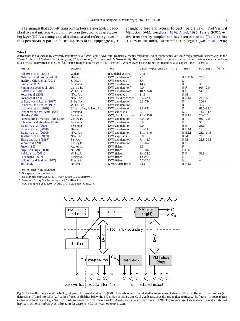
Fig. 1. Carbon flux diagram of the biological pump. Fish-mediated export (FME), the carbdefecation (Cd), and mortality (Cm) carbon fluxes of all fishes below the 150 m flux boundcarbon of detrital origin, Cdo = A(A + B)�1, is defined in terms of the fluxes marked A and Bhere. An additional carbon export flux term for excretion (Ce) is shown for zooplankton

at night to feed and returns to depth before dawn (Diel VerticalMigration, DVM; Longhurst, 1976; Angel, 1985; Pearre, 2003). Ac-tive transport by zooplankton has been estimated (Table 1), butstudies of the biological pump either neglect (Karl et al., 1996;

vertically migratory and ontogenetically vertically migratory taxa respectively. In thetality. The first row of the table is a global carbon export estimate made with the Lawshere given by the author, estimated passive export (‘‘POC’’) is listed.

Carbon export (mg C m�2 d�1) Terms POC (mg C m�2 d�1)

ort 91.6 – –ktona 7.1 R, E, F, M 23.7s 8.4 M –e

kton 14.5 R 39ktonb 4.0 R, F 9.5–12.0ktonc 10.2–24.8 R, F 54.8s 11.8 R, M –e

pepods 9.4–22.4 R, F, M 23.1–61.8kton 6.3–7.9 R 204.0kton 3.1 R 49.2ktona 2.8–8.8 R 64.0–86.0s 0.3 M 13.2–33.4pepods 7.3–133.0 R, F, M 20–315

kton 4.0–7.0 R 9.5–12.0kton 0.9 F 30kton 2.0 R, E 25.6kton 3.2–13.6 R, E, M 18kton 31.1–91.6 R, E, M 23.1–61.8s 8.0 R, M 22.3

kton 7.1–12.7 R, M 22.8–28.8kton 2.3–8.4 R, F 15.8

2.5 F –0.1–0.6 E, F, M –8.4–24.0 R, F 54.812.5d F –5.7–20.3 M –

shes 23.9 R, F, M –

on export mediated by mesopelagic fishes, is defined as the sum of respiratory (Cr),ary and Cd of VM fishes above the 150 m flux boundary. The fraction of zooplanktonand is not counted towards FME. Only mesopelagic fishes (shaded boxes) are studied.

16 P.C. Davison et al. / Progress in Oceanography 116 (2013) 14–30

Emerson et al., 1997; Falkowski et al., 2003; Buesseler et al.,2007a,b; Buesseler and Boyd, 2009) or minimize (Angel, 1989a,b;Longhurst and Harrison, 1989; Longhurst et al., 1990) the role ofmicronekton. Fishes are an important subcategory of mesopelagicmicronekton whose abundance has been underestimated byapproximately an order of magnitude due to low capture efficiency(Barkley, 1972; Koslow et al., 1997; Davison, 2011; Kaartvedt et al.,2012). Two modern point estimates of active transport by mesope-lagic fishes using abundance corrected for capture efficiency showthat carbon export by fishes can be as much as 28% of the total flux,and can exceed 20 mg C m�2 d�1 (Table 1; Williams and Koslow,1997; Hidaka et al., 2001).

We combined observations of water temperature and fish bio-mass, size distribution, and migratory behavior over a broad regionof the northeast Pacific Ocean with published physiological andecological rates to estimate the carbon export out of the epipelagicthat is mediated by mesopelagic fishes (‘‘fish-mediated export’’;FME; Fig. 1). FME was then compared to the passive flux and to to-tal carbon export estimated from satellite-derived measurementsof net primary productivity (NPP), sea surface temperature, anddepth of the euphotic zone. The regression between FME and satel-lite-derived total export was used to estimate FME for the entirestudy area.

2. Methods

2.1. Collection of fishes

Mesopelagic fishes were collected in 2008 and 2009 from 77stations on cruises of the R/V Melville (cruise P0810 of the Califor-nia Current Ecosystem Long Term Ecological Research program), R/V New Horizon (‘‘SEAPLEX’’), and the National Oceanic and

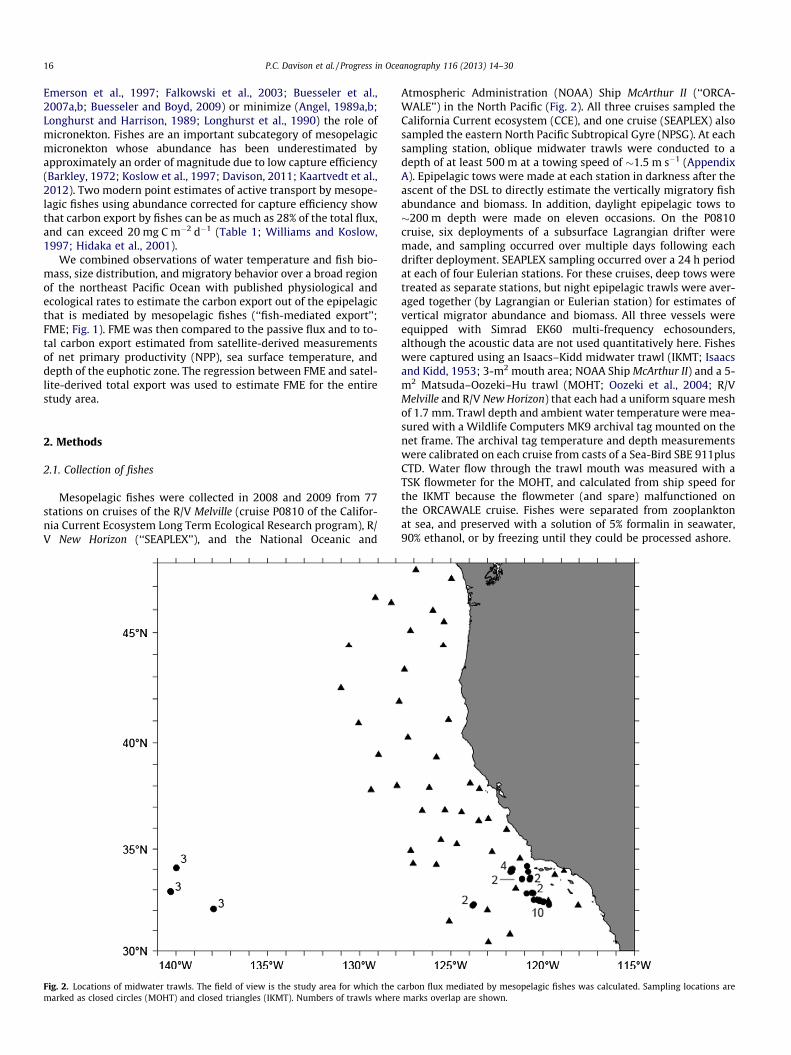
Fig. 2. Locations of midwater trawls. The field of view is the study area for which the cmarked as closed circles (MOHT) and closed triangles (IKMT). Numbers of trawls where

Atmospheric Administration (NOAA) Ship McArthur II (‘‘ORCA-WALE’’) in the North Pacific (Fig. 2). All three cruises sampled theCalifornia Current ecosystem (CCE), and one cruise (SEAPLEX) alsosampled the eastern North Pacific Subtropical Gyre (NPSG). At eachsampling station, oblique midwater trawls were conducted to adepth of at least 500 m at a towing speed of �1.5 m s�1 (AppendixA). Epipelagic tows were made at each station in darkness after theascent of the DSL to directly estimate the vertically migratory fishabundance and biomass. In addition, daylight epipelagic tows to�200 m depth were made on eleven occasions. On the P0810cruise, six deployments of a subsurface Lagrangian drifter weremade, and sampling occurred over multiple days following eachdrifter deployment. SEAPLEX sampling occurred over a 24 h periodat each of four Eulerian stations. For these cruises, deep tows weretreated as separate stations, but night epipelagic trawls were aver-aged together (by Lagrangian or Eulerian station) for estimates ofvertical migrator abundance and biomass. All three vessels wereequipped with Simrad EK60 multi-frequency echosounders,although the acoustic data are not used quantitatively here. Fisheswere captured using an Isaacs–Kidd midwater trawl (IKMT; Isaacsand Kidd, 1953; 3-m2 mouth area; NOAA Ship McArthur II) and a 5-m2 Matsuda–Oozeki–Hu trawl (MOHT; Oozeki et al., 2004; R/VMelville and R/V New Horizon) that each had a uniform square meshof 1.7 mm. Trawl depth and ambient water temperature were mea-sured with a Wildlife Computers MK9 archival tag mounted on thenet frame. The archival tag temperature and depth measurementswere calibrated on each cruise from casts of a Sea-Bird SBE 911plusCTD. Water flow through the trawl mouth was measured with aTSK flowmeter for the MOHT, and calculated from ship speed forthe IKMT because the flowmeter (and spare) malfunctioned onthe ORCAWALE cruise. Fishes were separated from zooplanktonat sea, and preserved with a solution of 5% formalin in seawater,90% ethanol, or by freezing until they could be processed ashore.

arbon flux mediated by mesopelagic fishes was calculated. Sampling locations aremarks overlap are shown.


In the laboratory, fishes were identified to species, the standardlength (LS) was measured to the nearest mm, and the wet weightwas measured to a precision of 0.01 g or calculated from alength–weight curve constructed from a subset of the material.Fishes of the genus Cyclothone were weighed in aggregate by spe-cies to save time because they often numbered several hundred pertrawl, and mean weights of Cyclothone spp. were used for meta-bolic modeling. Each fish species was classified as either ‘‘verticallymigratory’’ (VM) or ‘‘non-migratory’’ (NM) according to our owndata and references from the literature. VM fishes included Vinci-guerria spp., Scopelarchus spp., Diplophos taenia, Bregmaceros japo-nicus, all Bathylagidae (except Bathylagus pacificus andPseudobathylagus milleri), and all Myctophidae except Protomyctop-hum spp., Taaningichthys bathyphilus, Stenobrachius nannochir, Par-vilux ingens, Nannobrachium regale, Nannobrachium bristori,Nannobrachium fernae, and Nannobrachium lineatum (Childressand Nygaard, 1973; Wisner, 1976; Pearcy et al., 1977).

Most small mesopelagic fishes consume pelagic crustaceansand/or other zooplankton (Hopkins and Baird, 1977; Gjosaeterand Kawaguchi, 1980; Hopkins et al., 1996). Fishes assumed tobe piscivorous (most fishes of the family Stomiidae, plus singlelarge specimens each of Benthalbella dentata and Lamprogrammusniger) were excluded from the analysis because their ingestion ofcarbon is included in the mortality term of other mesopelagicfishes. The stomiids Tactostoma macropus, Bathophilus flemingi,Malacosteus niger, and Photostomias sp. were considered to beplanktivores (Borodulina, 1972; Clarke, 1982) and included in allanalyses. Larval and epipelagic fishes were not included in model-ing or analysis, and are not considered further.

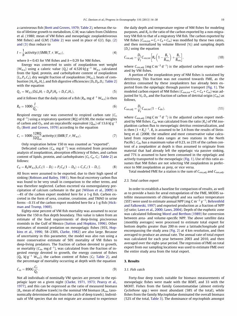
2.2. Carbon flux mediated by mesopelagic fishes (FME)

The overall carbon flux model for an individual mesopelagic fishwas constructed from an energy budget. The daily energy usage(kJ d�1) of a fish was calculated for a 24 h period in 1 min incre-ments from its size, temperature, diel activity pattern, and routinemetabolic rate. The energy budget equation was then solved foringestion rate, which was then converted to units of carbon(mg C d�1), as described below. Each fish from each deep trawlwas modeled, and then carbon flux was summed for all fisheswithin a trawl. Carbon fluxes modeled for individual trawl catcheswere adjusted for capture efficiency of the IKMT (relative to theMOHT) and the MOHT (relative to concurrent acoustic biomassestimates; Davison, 2011). The annual rate of carbon export wascalculated by multiplying the modeled daily rate by 365. Symbolsused for model terms are listed in Table 2.

VM fishes were assumed to feed in the epipelagic at night. Thecontribution of NM fishes to carbon export here is via consumptionof VM zooplankton, and thus this term is a subset of zooplanktonmortality export flux (Fig. 1).

The model estimates carbon flux across a 150-m depth horizon(chosen as a conventional depth of both sediment trap samplingand of the epipelagic layer) over a 24-h period partitioned into res-piration, fecal, and mortality categories. The most appropriatedepth to use for a flux boundary is likely variable (Buesseler andBoyd, 2009), but the model here is not sensitive to the precise loca-tion of this boundary because all fishes are assumed inhabit adepth of 400 m during the day, with the VM fishes assumed to as-cend to 50 m at night.

All fishes were assumed to inhabit a depth of 400 m during theday and to experience the measured temperature there. VM fisheswere assumed to ascend to 50 m at night where they experiencethe mean epipelagic temperature (1–150 m). Temperature is as-sumed to vary linearly between 50 m and 400 m depths. Thisassumption introduces a maximum error of �2.5 �C during DVM,and affects FME estimates by <2%. The densest portion of the

(daytime) 38 kHz DSL is at approximately 400 m in the study area,as observed from concurrently collected acoustic data. Less-denselayers were often observed both above and below the 400 m layer.Temperature changes slowly (by �0.01 �C m�1) at 400 m, and low-er metabolic rates of fishes below 400 m will be offset by highermetabolic rates of fishes above 400 m. We view the choice of400 m as the daytime depth of mesopelagic fishes to be bothappropriate and conservative for carbon export calculations be-cause the densest portion of the DSL was observed acoustically atapproximately 400 m, biomass generally decreases with depth,temperature increases more quickly from 400 to 150 m depth thanit decreases deeper than 400 m, and because the effort to verticallymigrate deeper than 400 m will offset the effect on metabolic ratefrom slowly decreasing temperatures. Because VM fishes are dis-tributed throughout the epipelagic at night (Pearcy et al., 1977),the choice of 50 m as their night depth represents a compromisebetween the observed dense acoustic layer from �10 to 50 mand the bottom of the epipelagic zone. The model is not sensitiveto this depth choice, as the mean epipelagic temperature is usedand the night depth is only used to estimate swimming effort.

VM fishes were assumed to ascend and descend at 5 cm s�1

(Table A1) from 400 m to 50 m in depth (transit time of �2 h) witha swimming speed of 2 body lengths (BL) s�1. The observed slope ofthe 38 kHz DSL was consistent with this vertical velocity assump-tion. The energetically optimal (by distance traveled) swimmingspeed for fishes of 0.1–10.0 g wet weight (Ww,f) ranges from 4.0to 2.1 BL s�1 (Videler, 1993). The amount to which VM fishes areable to manipulate buoyancy to reduce energy expenditure duringvertical migration is unknown. As energy expenditure, and thus re-spired carbon, increases exponentially with swimming speed inunits of BL s�1, selection of the lower bound in swimming speedis conservative in terms of carbon export.

The routine metabolic rate (RMR, kJ min�1) of fishes was as-sumed to be a function of fish wet weight (Ww,f) and temperature(T) following Gillooly et al. (Gillooly et al., 2001),

RMR ¼ 0:001eaW0:75w;f eð

1000c273:15þTÞ; ð1Þ

where a = 14.47 and c = �5.020. The standard metabolic rate (SMR,kJ min�1) of resting, inactive fishes is assumed to be 50% of the RMR(Winberg, 1956). The active, feeding metabolic rate (AMR, kJ min�1)is assumed to be four times the SMR (Brett and Groves, 1979; Smithand Laver, 1981). Because the metabolic rate of fishes decreaseswith the depth inhabited (in addition to temperature effects), themetabolic rates of NM fishes were reduced by an additional factorof 0.49 corresponding to the ratio of RMR between 400 and 50 mresidence depths (Torres et al., 1979). Both VM and NM fishes(Smith and Laver, 1981) were assumed to spend half of a 24 h per-iod actively feeding with a metabolic rate equivalent to the AMRand half of the day inactive with a metabolic rate equal to the SMR.

Few data are available concerning the physiological energeticsof mesopelagic fishes (Childress et al., 1980), as they are notori-ously difficult to keep alive in captivity (Robison, 1973). Giventhe lack of detailed knowledge, the annual time scale assumed be-low, the large number of mesopelagic fish species, and the widevariety of size classes considered, the use of generalized energybudgets was deemed appropriate. The general balanced energyequation for a fish can be expressed as follows (Brett and Groves,1979; Jobling, 1993):

I ¼ MðI; T;Ww;f Þ þ GðIÞ þ FðIÞ þ EðIÞ; ð2Þ

with

M ¼ activityðtÞSMRðT; r;Ww;f Þ þ SDAðIÞ; ð3Þ

where I is the ingestion rate (kJ d�1), M the metabolic rate (kJ d�1), Tthe temperature (�C), r the residence depth (m), G the growth rate

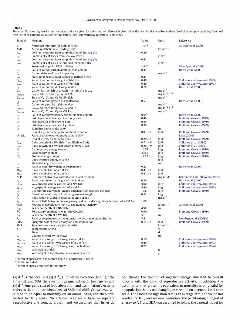
Table 2Notation. No value is given if a term varies, no units are given for ratios, and no reference is given when the term is calculated from others. Symbol subscripts containing ‘‘nm’’ and‘‘vm’’ refer to differing values for non-migratory (NM) and vertically migratory (VM) fishes.

Symbol Meaning Value Units Reference

a Regressed intercept for RMR of fishes 14.47 Gillooly et al. (2001)AMR Active metabolic rate (feeding fish) kJ min�1

bnm Constant resulting from simplification of Eqs. (2), (3) 0.29Bs Biomass of VM fishes from shallow trawls g m�2

bvm Constant resulting from simplification of Eqs. (2), (3) 0.43Bvm Biomass of VM fishes determined taxonomically g m�2

c Regressed slope for RMR of fishes �5.02 Gillooly et al. (2001)Cc Ratio of carbon:carbohydrate of zooplankton 0.44 Harris et al. (2000)Cd Carbon defecated by a fish per day mg d�1

Cdo Fraction of zooplankton carbon of detrital origin 0.23Cf,nm Ratio of carbon:wet weight of NM fish 0.40c Childress and Nygaard (1973)Cf,vm Ratio of carbon:wet weight of VM fish 0.49c Childress and Nygaard (1973)Cl Ratio of carbon:lipid of zooplankton 0.78 Harris et al. (2000)Cm Carbon lost by fish to growth (mortality) per day mg d�1

Cnm,adj Cnm,tot adjusted for Cdo, Vf, and Ds mg m�2 d�1

Cnm,tot Sum of Cm, Cr, and Cd for NM fish mg d�1

Cp Ratio of carbon:protein of zooplankton 0.53 Harris et al. (2000)Cr Carbon respired by a fish per day mg d�1

Cvm,adj Cvm,tot adjusted for Bs:Bvm, Vf, and Ds mg m�2 d�1

Cvm,tot Sum of Cm, Cr, and Cd for VM fish mg d�1

Cz Ratio of carbohydrate:dry weight of zooplankton 0.05b Harris et al. (2000)Dc Fish digestive efficiency of carbohydrate 0.40 Brett and Groves (1979)Dl Fish digestive efficiency of lipid 0.85 Brett and Groves (1979)Dp Fish digestive efficiency of protein 0.90 Brett and Groves (1979)Ds Sampling depth of the trawl mE Loss of ingested energy to non-fecal excretion 0.07 � I kJ d�1 Brett and Groves (1979)ef ratio Ratio of total exported production to NPP Laws (2004)F Loss of ingested energy to feces 0.20 � I kJ d�1 Brett and Groves (1979)Gnm Daily growth of a NM fish (from lifetime G:M) 0.71 �M kJ d�1 Childress et al. (1980)Gvm Daily growth of a VM fish (from lifetime G:M) 0.28 �M kJ d�1 Childress et al. (1980)Hc Carbohydrate energy content 16.74 kJ g�1 Brett and Groves (1979)Hl Lipid energy content 39.55 kJ g�1 Brett and Groves (1979)Hp Protein energy content 18.25 kJ g�1 Brett and Groves (1979)I Daily ingested energy of a fish kJ d�1

Ls Standard length of a fish mmLz Ratio of lipid:dry weight of zooplankton 0.22 Harris et al. (2000)Mnm Daily metabolism of a NM fish 0.43 � I kJ d�1

Mvm Daily metabolism of a VM fish 0.57 � I kJ d�1

NPP Difference between autotrophic fixed and respired C mg m2 d�1 Behrenfeld and Falkowski (1997)Pz Ratio of protein:dry weight of zooplankton 0.50 Harris et al. (2000)Qf,nm Ww,f-specific energy content of a NM fish 3.06c kJ g�1 Childress and Nygaard (1973)Qf,vm Ww,f-specific energy content of a VM fish 5.84c kJ g�1 Childress and Nygaard (1973)Qox Oxycalorific equivalent (energy obtained from respired oxygen) 13.6 kJ g�1 Brett and Groves (1979)Qz Caloric value of zooplankton per gram wet weight 4.52 kJ g�1

Rd Daily ration of a fish, expressed in units of Ww,z mg d�1

Re Ratio of FME between non-migratory and vertically migratory behavior of a VM fish 1.06RMR Routine metabolic rate (normal spontaneous activity) kJ min�1 Gillooly et al. (2001)rnm Residence depth of a NM fish 400 mRQ Respiratory quotient (molar ratio CO2:O2) 0.90 Brett and Groves (1979)rvm Residence depth of a VM fish 50 mRz Ratio of zooplankton active transport to detritus remineralization 3.4 Steinberg et al. (2008b)SDA Energetic cost of food absorption and assimilation 0.14 � I kJ d�1 Brett and Groves (1979)SMR Standard metabolic rate (torpid fish) kJ min�1

T Temperature of fish �Ct Time dVf Volume filtered by the trawl mc

Wd,f,nm Ratio of dry weight:wet weight of a NM fish 0.18c Childress and Nygaard (1973)Wd,f,vm Ratio of dry weight:wet weight of a VM fish 0.26c Childress and Nygaard (1973)Wd,z Ratio of dry weight:wet weight of zooplankton 0.21a Childress and Nygaard (1974)Ww,f Wet weight of fish gWw,z Wet weight of zooplankton consumed by a fish g

a Mean of species with minimum depth of occurrence 6400 m.b Chitin included.c Mean of species captured in this study.


(kJ d�1), F the fecal loss (kJ d�1), E non-fecal excretion (kJ d�1), t thetime (d), and SDA the specific dynamic action or heat increment(kJ d�1; energetic cost of food absorption and assimilation). Activityrefers to the time-partitioned use of SMR and AMR. Growth was as-sumed to be equal to mortality on an annual basis, and then con-verted to daily units. No attempt was made here to separatereproductive and somatic growth, and we assumed that fishes do

not change the fraction of ingested energy allocated to overallgrowth with the onset of reproductive activity. In addition, theassumption that growth is equivalent to mortality is only valid fora population that is not changing in size and on a generational timescale. The calculated ingestion rate is an average rate, and we do notresolve its daily and seasonal variation. The partitioning of ingestedenergy to F, E, and SDA was assumed to follow the general model for


a carnivorous fish (Brett and Groves, 1979; Table 2), whereas the ra-tio of lifetime growth to metabolism, G:M, was taken from Childresset al. (1980; mean of VM fishes and mesopelagic zooplanktivorousNM fishes) and G(M) (Table 2) was used in place of G(I). Eqs. (2)and (3) thus reduce to

I ¼ 1b

activityðtÞSMRðT; r;Ww;fÞ; ð4Þ

where b = 0.43 for VM fishes and b = 0.29 for NM fishes.Energy was converted to units of zooplankton wet weight

(Ww,z) using a caloric value (Qz) of 4.520 kJ g�1 Ww,z calculatedfrom the lipid, protein, and carbohydrate content of zooplankton(Lz,Pz,Cz), dry weight fraction of zooplankton (Wd,z), heats of com-bustion (Hl,Hp,Hc), and fish digestive efficiencies (Dl,Dp,Dc; Table 2)with the equation

Q z ¼Wd;zðDlLzHl þ DpPzHp þ DcCzHcÞ; ð5Þ

and it follows that the daily ration of a fish (Rd, mg d�1 Ww,z) is then

Rd ¼ 1000I

Q z: ð6Þ

Respired energy rate was converted to respired carbon rate (Cr,mg d�1) using a respiratory quotient (RQ) of 0.90, the molar weightsof carbon and O2, and an oxycalorific equivalent (Qox) of 13.6 kJ g�1

O2 (Brett and Groves, 1979) according to the equation

Cr ¼ 100012RQ32Q ox

activityðtÞSMRðT; r;Ww;f Þ: ð7Þ

Only respiration below 150 m was counted as ‘‘exported’’.Defecated carbon (Cd, mg d�1) was estimated from proximate

analysis of zooplankton, absorption efficiency of fishes, and carboncontent of lipids, protein, and carbohydrates (Cl, Cp, Cc; Table 2) asfollows:

Cd ¼ RdWd;z½LzClð1� DlÞ þ PzCpð1� DpÞ þ CzCcð1� DcÞ�: ð8Þ

All feces were assumed to be exported, due to their high speed ofsinking (Robison and Bailey, 1981). Non-fecal excretory carbon fluxwas found to be very small in comparison to the other terms, andwas therefore neglected. Carbon excreted via osmoregulatory pre-cipitation of calcium carbonate in the gut (Wilson et al., 2009) is�4% of the carbon export modeled here for a 1-g fish. Carbon ex-creted in the form of urea, creatine, creatinine, and TMAO in urineforms �0.1% of the carbon export modeled here for a 1-g fish (Hick-man and Trump, 1969).

Eighty-nine percent of VM fish mortality was assumed to occurbelow the 150 m flux depth boundary. This value is taken from anestimate of the food requirements of deep-living piscivorousstomiids in the Gulf of Mexico (Sutton and Hopkins, 1996). Otherestimates of stomiid predation on mesopelagic fishes (95%, Hop-kins et al., 1996; 58–230%, Clarke, 1982) are also large. Becauseof uncertainty in this parameter, the model was also run using amore conservative estimate of 50% mortality of VM fishes todeep-living predators. The fraction of carbon devoted to growth,or mortality (Cm, mg d�1), was calculated from the fraction of in-gested energy devoted to growth, the energy content of fishes(Qf, kJ g�1 Ww,f), the carbon content of fishes (Cf; Table 2), andthe percentage of mortality occurring at depth with the equation

Cm ¼ 890GCf

Q f: ð9Þ

Not all individuals of nominally VM species are present in the epi-pelagic layer on a given night (Clarke, 1971, 1973; Pearcy et al.,1977), and this can be expressed as the ratio of measured biomass(Bs, mean of shallow trawls) to the nominal VM biomass (Bvm, taxo-nomically determined mean from the catch of deep trawls). Individ-uals of VM species that do not migrate are assumed to experience

the daily depth and temperature regime of NM fishes for modelingpurposes, and Re is the ratio of the carbon exported by a non-migra-tory VM fish to that of a migratory VM fish. The carbon exported byVM fishes (Cvm,tot = Cr + Cd + Cm) was modified by these two ratios,and then normalized by volume filtered (Vf) and sampling depth(Ds) using the equation

Cvm;adj ¼Ds

V fCvm;tot Re 1� Bs

Bvm

� �þ Bs

Bvm

� �; ð10Þ

where Cvm,adj (mg C m�2 d�1) is the adjusted carbon export medi-ated by VM fishes.

A portion of the zooplankton prey of NM fishes is sustained bydetritivory. This fraction was not counted towards FME, as thedetritus consumed by these zooplankters has already been ex-ported from the epipelagic through passive transport (Fig. 1). Themodeled carbon export of NM fishes (Cnm,tot = Cr + Cd + Cm) was ad-justed for Vf, Ds, and the fraction of carbon of detrital origin (Cdo) asfollows,

Cnm;adj ¼Ds

V fCnm;totð1� CdoÞ; ð11Þ

where Cnm,adj (mg C m�2 d�1) is the adjusted carbon export medi-ated by NM fishes. Cdo was calculated from the ratio (Rz) of VM zoo-plankton carbon flux to mesopelagic detritus remineralization, andis then (1 + Rz)�1. Rz is assumed to be 3.4 from the results of Stein-berg et al. (2008; the smallest and most conservative value calcu-lated from reported data ranges at two stations in the NorthPacific). Cdo has a maximum value of 0.23, so 23% of the carbon con-tent of a zooplankter at depth is thus assumed to originate frommaterial that had already left the epipelagic via passive sinking,and 77% is assumed to have been consumed in the epipelagic andactively transported to the mesopelagic (Fig. 1). Use of this ratio as-sumes that NM fishes are not selecting VM zooplankton in prefer-ence to NM zooplankton as prey, or vice versa.

Total modeled FME for a station is the sum of Cvm,adj and Cnm,adj.

2.3. Total carbon export

In order to establish a baseline for comparison of results, as wellas to provide a basis for areal extrapolation of the FME, MODIS sa-tellite measurements of chlorophyll and sea surface temperature(SST) were used to estimate annual NPP (mg C m�2 y�1; Behrenfeldand Falkowski, 1997) and exported production as a fraction of NPP(ef ratio; Laws et al., 2000; Laws, 2004). Depth of the euphotic zonewas calculated following Morel and Berthon (1989) for conversionbetween area- and volume-specific NPP. The above satellite data(monthly averages) were processed to estimate total export forbottom depths greater than 200 m over a latitude/longitude gridencompassing the study area (Fig. 2) at 4 km resolution, and thenaveraged to produce an annual rate. The annual rate of total exportwas calculated for each year between 2003 and 2010, and thenaveraged over the eight-year period. The regression of FME on totalexport from our sampling locations was used to estimate FME overthe entire study area from the total export.

3. Results

3.1. Fish catch

Forty-four deep trawls suitable for biomass measurements ofmesopelagic fishes were made with the IKMT, and 33 with theMOHT. Fishes from the family Gonostomatidae (almost entirelyCyclothone spp.) were most abundant (58% of the total), whilefishes from the family Myctophidae dominated the overall biomass(52% of the total, Table 3). The dominance of myctophids amongst

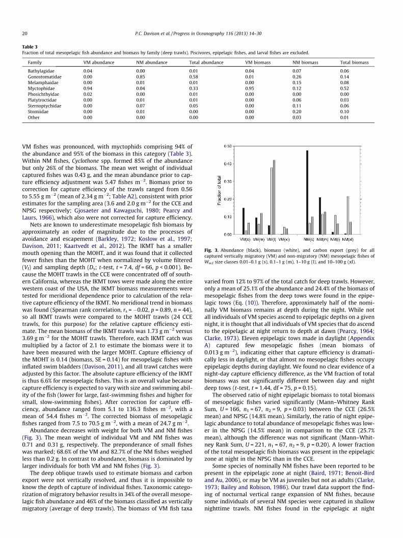
Table 3Fraction of total mesopelagic fish abundance and biomass by family (deep trawls). Piscivores, epipelagic fishes, and larval fishes are excluded.

Family VM abundance NM abundance Total abundance VM biomass NM biomass Total biomass

Bathylagidae 0.04 0.00 0.01 0.04 0.07 0.06Gonostomatidae 0.00 0.85 0.58 0.01 0.26 0.14Melamphaidae 0.00 0.01 0.01 0.00 0.15 0.08Myctophidae 0.94 0.04 0.33 0.95 0.12 0.52Phosichthyidae 0.02 0.00 0.01 0.00 0.00 0.00Platytroctidae 0.00 0.01 0.01 0.00 0.06 0.03Sternoptychidae 0.00 0.07 0.05 0.00 0.11 0.06Stomiidae 0.00 0.01 0.00 0.00 0.20 0.10Other 0.00 0.00 0.00 0.00 0.03 0.01

Fig. 3. Abundance (black), biomass (white), and carbon export (grey) for allcaptured vertically migratory (VM) and non-migratory (NM) mesopelagic fishes ofWw,f size classes 0.01–0.1 g (s), 0.1–1 g (m), 1–10 g (l), and 10–100 g (xl).


VM fishes was pronounced, with myctophids comprising 94% ofthe abundance and 95% of the biomass in this category (Table 3).Within NM fishes, Cyclothone spp. formed 85% of the abundancebut only 26% of the biomass. The mean wet weight of individualcaptured fishes was 0.43 g, and the mean abundance prior to cap-ture efficiency adjustment was 5.47 fishes m�2. Biomass prior tocorrection for capture efficiency of the trawls ranged from 0.56to 5.55 g m�2 (mean of 2.34 g m�2; Table A2), consistent with priorestimates for the sampling area (3.6 and 2.0 g m�2 for the CCE andNPSG respectively; Gjosaeter and Kawaguchi, 1980; Pearcy andLaurs, 1966), which also were not corrected for capture efficiency.

Nets are known to underestimate mesopelagic fish biomass byapproximately an order of magnitude due to the processes ofavoidance and escapement (Barkley, 1972; Koslow et al., 1997;Davison, 2011; Kaartvedt et al., 2012). The IKMT has a smallermouth opening than the MOHT, and it was found that it collectedfewer fishes than the MOHT when normalized by volume filtered(Vf) and sampling depth (Ds; t-test, t = 7.4, df = 66, p < 0.001). Be-cause the MOHT trawls in the CCE were concentrated off of south-ern California, whereas the IKMT tows were made along the entirewestern coast of the USA, the IKMT biomass measurements weretested for meridional dependence prior to calculation of the rela-tive capture efficiency of the IKMT. No meridional trend in biomasswas found (Spearman rank correlation, rs = �0.02, p = 0.89, n = 44),so all IKMT trawls were compared to the MOHT trawls (24 CCEtrawls, for this purpose) for the relative capture efficiency esti-mate. The mean biomass of the IKMT trawls was 1.73 g m�2 versus3.69 g m�2 for the MOHT trawls. Therefore, each IKMT catch wasmultiplied by a factor of 2.1 to estimate the biomass were it tohave been measured with the larger MOHT. Capture efficiency ofthe MOHT is 0.14 (biomass, SE = 0.14) for mesopelagic fishes withinflated swim bladders (Davison, 2011), and all trawl catches wereadjusted by this factor. The absolute capture efficiency of the IKMTis thus 6.6% for mesopelagic fishes. This is an overall value becausecapture efficiency is expected to vary with size and swimming abil-ity of the fish (lower for large, fast-swimming fishes and higher forsmall, slow-swimming fishes). After correction for capture effi-ciency, abundance ranged from 5.1 to 136.3 fishes m�2, with amean of 54.4 fishes m�2. The corrected biomass of mesopelagicfishes ranged from 7.5 to 70.5 g m�2, with a mean of 24.7 g m�2.

Abundance decreases with weight for both VM and NM fishes(Fig. 3). The mean weight of individual VM and NM fishes was0.71 and 0.31 g, respectively. The preponderance of small fisheswas marked; 68.6% of the VM and 82.7% of the NM fishes weighedless than 0.2 g. In contrast to abundance, biomass is dominated bylarger individuals for both VM and NM fishes (Fig. 3).

The deep oblique trawls used to estimate biomass and carbonexport were not vertically resolved, and thus it is impossible toknow the depth of capture of individual fishes. Taxonomic catego-rization of migratory behavior results in 34% of the overall mesope-lagic fish abundance and 46% of the biomass classified as verticallymigratory (average of deep trawls). The biomass of VM fish taxa

varied from 12% to 97% of the total catch for deep trawls. However,only a mean of 25.1% of the abundance and 24.4% of the biomass ofmesopelagic fishes from the deep tows were found in the epipe-lagic tows (Eq. (10)). Therefore, approximately half of the nomi-nally VM biomass remains at depth during the night. While notall individuals of VM species ascend to epipelagic depths on a givennight, it is thought that all individuals of VM species that do ascendto the epipelagic at night return to depth at dawn (Pearcy, 1964;Clarke, 1973). Eleven epipelagic tows made in daylight (AppendixA) captured few mesopelagic fishes (mean biomass of0.013 g m�2), indicating either that capture efficiency is dramati-cally less in daylight, or that almost no mesopelagic fishes occupyepipelagic depths during daylight. We found no clear evidence of anight-day capture efficiency difference, as the VM fraction of totalbiomass was not significantly different between day and nightdeep tows (t-test, t = 1.44, df = 75, p = 0.15).

The observed ratio of night epipelagic biomass to total biomassof mesopelagic fishes varied significantly (Mann–Whitney RankSum, U = 166, n1 = 67, n2 = 9, p = 0.03) between the CCE (26.5%mean) and NPSG (14.8% mean). Similarly, the ratio of night epipe-lagic abundance to total abundance of mesopelagic fishes was low-er in the NPSG (14.5% mean) in comparison to the CCE (25.7%mean), although the difference was not significant (Mann–Whit-ney Rank Sum, U = 221, n1 = 67, n2 = 9, p = 0.20). A lower fractionof the total mesopelagic fish biomass was present in the epipelagiczone at night in the NPSG than in the CCE.

Some species of nominally NM fishes have been reported to bepresent in the epipelagic zone at night (Baird, 1971; Benoit-Birdand Au, 2006), or may be VM as juveniles but not as adults (Clarke,1973; Bailey and Robison, 1986). Our trawl data support the find-ing of nocturnal vertical range expansion of NM fishes, becausesome individuals of several NM species were captured in shallownighttime trawls. NM fishes found in the epipelagic at night


formed 6.9% of the abundance and 12.7% of the biomass of the shal-low tows. These fishes were not present in shallow trawls to thesame depth conducted in daylight. For carbon export purposes,the presence of these fishes in the epipelagic zone at night partiallyoffsets the fishes from VM species that do not migrate.

The modeled FME by VM fishes was adjusted for the differencebetween taxonomic and trawl-based estimates of the verticallymigratory biomass (Eq. (10)). This adjustment is approximate, asit includes the small fraction of NM fishes found in the epipelagicwhich have (on average) lower metabolic rates, and it does not re-solve size- and species-specific differences in DVM behavior. Theadjustment is also small, as the ratio of carbon export by a non-migrating VM fish to that of a migrating VM fish is 1.06 (Table 4).

3.2. Individual FME model

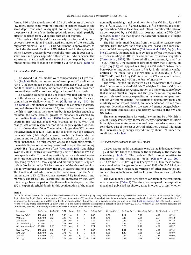
The VM and NM FME models were compared using a 1-g virtualfish (Table 4). Under a common set of assumptions (‘‘baseline sce-nario’’), the two models produce similar estimates of I, Rd, and car-bon flux (Table 4). The baseline scenario for each model was thenprogressively modified to the configuration used for analysis.

The baseline scenario of the VM model was first altered to re-flect the decreased energy available for growth by VM fishes incomparison to shallow-living fishes (Childress et al., 1980; Eq.(4); Table 2). This change directly reduces the estimated mortalityflux, and also results in decreased I, Rd, and defecation rate becausethe fish is respiring at the same rate but is not feeding enough tomaintain the same ratio of growth to metabolism assumed bythe baseline Brett and Groves (1979) budget. Second, the nightdepth in the VM fish model was changed to 50 m. With thischange, 72% of the respired carbon is no longer exported, as it oc-curs shallower than 150 m. The number is larger than 50% becausethe active metabolic rate (AMR; night) is higher than the standardmetabolic rate (SMR; day). Because thus far the temperature isconstant and vertical swimming has no metabolic cost, I and Rd re-main unchanged. The third change was to add swimming effort. Ifthe metabolic cost of swimming is assumed to equal the swimmingspeed (BL s�1) to an exponent of 2.5 (Alexander, 2003), and fishesswim at 2 BL s�1 with a vertical velocity 5 cm s�1, then the VM fishnow spends �4 h d�1 travelling vertically with an elevated meta-bolic rate equivalent to 6.7 times the SMR. This has the effect ofincreasing by 27% I, Rd, fecal export, and mortality export. Respiredcarbon flux increases by 68% because most of the elevated respira-tion for swimming occurs below the 150 m export threshold depth.The fourth and final adjustment to the model was to set the 50 mtemperature to 13 �C. This change increased I, Rd, fecal export, andmortality export by 31%. Respiratory flux increased by 10% withthis change because part of the thermocline is deeper than the150 m export threshold depth. In this configuration of the model,

Table 4Carbon flux model scenarios for a 1-g fish. The baseline scenarios for the vertically migratodepth (Dn) = day depth (Dd), night temperature (Tn) = day temperature (Td), no elevated memetabolic rate for residence depth (DE), prey detritivory fraction (Cdo) = 0, and the generaresults for daily energy requirement (I), daily ration (Rd), and carbon exported via respircumulatively modified to the configurations used to estimate FME (indicated with asteris

Scenario Dn:Dd (m) Td:Tn (�C) G:M Swim DE Cdo Cr (mg C

Baseline (VM) 400:400 7:7 0.66 No 1 0 1.42VM G:M 400:400 7:7 0.28 No 1 0 1.42Add ascent 50:400 7:7 0.28 No 1 0 0.40Add swimming 50:400 7:7 0.28 Yes 1 0 0.67Add warm surface⁄ 50:400 7:13 0.28 Yes 1 0 0.74

Baseline (NM) 400:400 7:7 0.66 No 1 0 1.42NM G:M 400:400 7:7 0.71 No 1 0 1.42Add DE 400:400 7:7 0.71 No 0.49 0 0.70Add Cdo

⁄ 400:400 7:7 0.71 No 0.49 0.23 0.54

nominally matching trawl conditions for a 1-g VM fish, Rd is 4.9%Ww,f d�1, I is 0.222 kJ d�1, and 2.12 mg C d�1 is exported, 35% as re-spired carbon, 32% as fecal flux, and 33% as mortality. The ratio ofcarbon exported by a VM fish that does not migrate (‘‘VM G:M’’scenario, Table 4) to that by one that ascends ‘‘normally’’ at night(Re, Eq. (10)) is 1.06.

The NM model modifications from the baseline scenario weresimpler. First, the G:M ratio was adjusted based upon measure-ments of NM mesopelagic fishes (Childress et al., 1980; Eq. (4), Ta-ble 2). Second, the metabolic rate by 49% to reflect the lower SMRof fishes residing at 400 m in comparison to vertical migrators(Torres et al., 1979). This lowered all export terms, Rd, and I by�50%. Third, Cdo, the fraction of consumed prey that is detrital inorigin (Eq. (11)) was applied, resulting in a 23% reduction to all car-bon export terms, but no change to I or Rd. In this nominal config-uration of the model for a 1-g NM fish, Rd is 2.2% Ww,f d�1, I is0.097 kJ d�1, and 1.29 mg C d�1 is exported, 42% as respired carbon,18% as fecal flux, and 40% in the form of mortality.

The overall carbon flux mediated by a 1-g NM fish is thus 61% ofthat from a similarly sized VM fish. The higher flux from VM fishesresults from a higher SMR, consumption of a higher fraction of preythat is non-detrital in origin, and the greater ration required tosupport elevated energy expenditures in warmer temperaturesand for vertical movement. The fractions of respiratory, fecal, andmortality carbon export (Table 4) are independent of size and tem-perature, depending wholly on the assumed energy budget, behav-ior, proximate compositions, and activity patterns of the VM andNM fishes.

The energy expenditure for vertical swimming by a VM fish is27% of its ingested energy. Increased energy expenditure resultingfrom higher temperatures encountered near the surface can also beconsidered part of the cost of vertical migration. Vertical migrationthus increases daily energy expenditure by about 67% under theconditions in Table 4.

3.3. Independent checks on the FME model

Carbon export model parameters were varied independently for1-g VM and NM fishes to determine the sensitivity of the model touncertainty (Table 5). The modeled FME is most sensitive toparameters of the respiration model (Gillooly et al., 2001;a = 14.47 and c = �5.02; Eq. (1)). Changes of ±1 SE in these param-eters resulted in changes to the estimated FME of 0.17–5.87 timesthe nominal value. Reasonable variation of other parameters re-sults in flux reductions of 24% or less and flux increases of 43%or less.

The FME model is most sensitive to variation of the respirationrate parameters (Table 5). Therefore, we compared the respirationmodel and published respiratory rates in order to assess whether

ry (VM) and non-migratory (NM) fish models use a common set of assumptions; nighttabolic rate for swimming between day and night depths (‘‘swim’’), no modification ofl growth:metabolism ratio (G:M; 0.66; Brett and Groves, 1979). The models produceation, defecation, and mortality (Cr, Cd, Cm respectively). The baseline scenarios are

ks).

d�1) Cd (mg C d�1) Cm (mg C d�1) Ctotal (mg C d�1) Rd (% Ww,f) I (kJ d�1)

0.58 1.11 3.11 4.22 0.1910.40 0.42 2.25 2.94 0.1330.40 0.42 1.23 2.94 0.1330.51 0.54 1.72 3.74 0.1690.68 0.70 2.12 4.92 0.222

0.58 1.31 3.31 4.22 0.1910.60 1.36 3.38 4.36 0.1970.30 0.67 1.67 2.15 0.0970.23 0.52 1.29 2.15 0.097

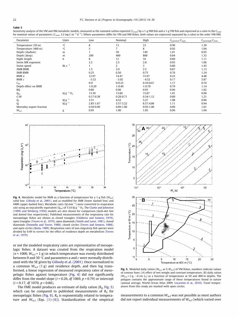
Table 5Sensitivity analysis of the VM and NM metabolic models, measured as the summed carbon exported (Ctotal) by a 1-g NM fish and a 1-g VM fish and expressed as a ratio to the Ctotal

for nominal values of parameters (Cnom, 3.2 mg C m�2 d�1). Where parameters differ for VM and NM fishes, both values are expressed separated by a colon in the order VM:NM.

Parameter Units Low Nominal High Ctotal,low:Cnom Ctotal,high:Cnom

Temperature (50 m) �C 8 13 23 0.90 1.30Temperature (400 m) �C 5 7 8 0.92 1.04Depth (shallow) m 1 50 149 1.01 0.95Depth (deep) m 200 400 800 0.84 1.33Night length h 8 12 16 0.89 1.11Swim MR exponent 2.2 2.5 2.8 0.95 1.06Swim speed BL s�1 1 2 3 0.80 1.43AMR:RMR 1.5 2.0 2.5 0.87 1.13SMR:RMR 0.25 0.50 0.75 0.76 1.24RMR a 12.97 14.47 15.97 0.22 4.48RMR c �5.52 �5.02 �4.52 0.17 5.87Cdo 0:0 0:0.23 0.10:0.67 1.17 0.76Depth effect on RMR 1:0.20 1:0.49 1:0.70 0.79 1.14RQ 0.80 0.90 0.95 0.96 1.02Qox kJ g�1 O2 13.39 13.60 15.07 1.01 0.96G:M 0.17:0.38 0.28:0.71 0.34:1.12 0.80 1.21Qz kJ g�1 3.51 4.52 5.27 1.08 0.96Qf kJ g�1 2.85:1.67 5.57:3.22 8.57:4.86 1.11 0.94Mortality export fraction 0.50:0.90 0.89:1.00 0.95:1.00 0.89 1.01Ww,f g 0.95 1.00 1.05 0.96 1.04

Fig. 4. Metabolic model for RMR as a function of temperature for a 1-g fish (Ww,f;solid line; Gillooly et al., 2001), and as modified for SMR (lower dashed line) andAMR (upper dashed line). Metabolic rates (kJ min�1) were converted to respirationrate using an oxycalorific equivalent (Qox) of 13.6 kJ g�1 O2. The Clarke and Johnston(1999) and Winberg (1956) models are also shown for comparison (dash-dot lineand dotted line respectively). Published measurements of the respiratory rate formesopelagic fishes are shown as closed triangles (Childress and Somero, 1979),open triangles (Torres et al., 1979), open diamonds (Smith and Laver, 1981), closeddiamonds (Donnelly and Torres, 1988), closed circles (Torres and Somero, 1988),and open circles (Ikeda, 1989). Respiration rates of non-migratory fish species weredivided by 0.49 to correct for the effect of residence depth on metabolism (Torreset al., 1979).

Fig. 5. Modeled daily ration (Ww,z as % Ww,f) of VM fishes, numbers indicate valuesof contour lines; (A) effect of wet weight and constant temperature, (B) daily ration(Ww,f = 2 g, �6 cm LS) as a function of temperature at 50 and 400 m depths. Thepolygon contains the approximate range of these temperatures found in nature(annual average, World Ocean Atlas 2009; Locarnini et al., 2010). Trawl temper-atures from this study are marked with open circles.


or not the modeled respiratory rates are representative of mesope-lagic fishes. A dataset was created from the respiration model(n = 1000, Ww,f = 1 g) in which temperature was evenly distributedbetween 0 and 30 �C and parameters a and c were normally distrib-uted with the SE given by Gillooly et al. (2001). Once normalized toa common Ww,f (1 g) and residence depth, and then log trans-formed, a linear regression of measured respiratory rates of meso-pelagic fishes against temperature (Fig. 4) did not significantlydiffer from the model slope (t = 0.26, df 1069, p = 0.79) or intercept(t = 0.17, df 1070, p = 0.86).

The FME model produces an estimate of daily ration (Rd, Fig. 5)which can be compared to published measurements of Rd formesopelagic fishes (Fig. 6). Rd is exponentially related to tempera-ture and Ww,f (Eqs. (1)–(6)). Standardization of the empirical

measurements to a common Ww,f was not possible as most authorsdid not report individual measurements of Ww,f (which varied over

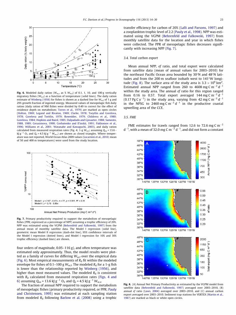
Fig. 6. Modeled daily ration (Ww,z as % Ww,f) of 0.1, 1, 10, and 100 g verticallymigratory fishes (Ww,f) as a function of temperature (solid lines). The daily rationestimate of Winberg (1956) for fishes is shown as a dashed line for Ww,f of 1 g and29% growth fraction of ingested energy. Measured values of mesopelagic fish dailyration (daily ration of NM fishes were divided by 0.49 to correct for the effect ofresidence depth on metabolism; Torres et al., 1979) are marked as open circles(Holton, 1969; Legand and Rivaton, 1969; Clarke, 1978; Tseytlin and Gorelova,1978; Gorelova and Tseitlin, 1979; Rowedder, 1979; Childress et al., 1980;Gorelova, 1984; Hopkins and Baird, 1985; Dalpadado and Gjosaeter, 1988; Sameoto,1988, 1989; Gerasimova, 1990; Gorbatenko and Il’inskii, 1991; Pakhomov et al.,1996; Williams et al., 2001; Watanabe and Kawaguchi, 2003), and daily rationcalculated from measured respiration rates (Fig. 4; 1-g Ww,f; assuming Qox = 13.6 -kJ g�1 O2 and Qz = 4.5 kJ g�1 Ww,z) are shown as closed triangles. Where temper-ature was not reported, World Ocean Atlas 2009 values (Locarnini et al., 2010; meanof 50 and 400 m temperatures) were used from the study location.

Fig. 7. Primary productivity required to support the metabolism of mesopelagicfishes (PPR; expressed as a percentage of NPP) assuming a trophic efficiency of 20%.NPP was estimated using the VGPM (Behrenfeld and Falkowski, 1997) from theannual mean of monthly satellite data. The Model I regression (solid line),geometric mean Model II regression (dash-dot line), 95% confidence intervals ofthe Model I regression (dotted lines), and Model I regression for 10% and 30%trophic efficiency (dashed lines) are shown.

Fig. 8. (A) Annual Net Primary Productivity as estimated by the VGPM model fromsatellite data (Behrenfeld and Falkowski, 1997) averaged over 2003–2010, (B)annual ef ratio (Laws, 2004) averaged over 2003–2010, and (C) annual carbonexport averaged over 2003–2010. Sediment trap stations for VERTEX (Martin et al.,1987) are marked as black or white open circles.


four orders of magnitude, 0.05–116 g), and often temperature wasestimated only approximately. Thus, the model results were plot-ted as a family of curves for differing Ww,f over the empirical data(Fig. 6). Most empirical measurements of Rd fit within the modeledenvelope for fishes of 0.1–100 g Ww,f. The modeled Rd for a 1-g fishis lower than the relationship reported by Winberg (1956), andhigher than most measured values. The modeled Rd is consistentwith Rd calculated from measured respiration rates (Figs. 4 and6) assuming Qox = 13.6 kJ g�1 O2 and Qz = 4.5 kJ g�1 Ww,z.

The fraction of annual NPP required to support the metabolismof mesopelagic fishes (primary productivity required, or PPR; Paulyand Christensen, 1995) was estimated at each sampling stationfrom modeled Rd following Barlow et al. (2008) using a trophic

transfer efficiency for carbon of 20% (Lalli and Parsons, 1997) anda zooplankton trophic level of 2.2 (Pauly et al., 1998). NPP was esti-mated using the VGPM (Behrenfeld and Falkowski, 1997) frommonthly satellite data for the location and year in which fisheswere collected. The PPR of mesopelagic fishes decreases signifi-cantly with increasing NPP (Fig. 7).

3.4. Total carbon export

Mean annual NPP, ef ratio, and total export were calculatedfrom satellite data (mean of annual values for 2003–2010) forthe northeast Pacific Ocean area bounded by 30�N and 48�N lati-tudes and from the 200 m seafloor isobath west to 141�W longi-tude (Fig. 8). The surface area of the study area is 3.3 � 106 km2.Estimated annual NPP ranged from 260 to 4608 mg C m�2 d�1

within the study area. The annual ef ratio for this region rangedfrom 0.16 to 0.57. Total export averaged 144 mg C m�2 d�1

(0.17 Pg C y�1) in the study area, varying from 42 mg C m�2 d�1

in the NPSG to 2460 mg C m�2 d�1 in the productive coastalupwelling area of the CCE.

3.5. FME

FME estimates for trawls ranged from 12.6 to 72.6 mg C m�2

d�1, with a mean of 32.0 mg C m�2 d�1, and did not form a constant

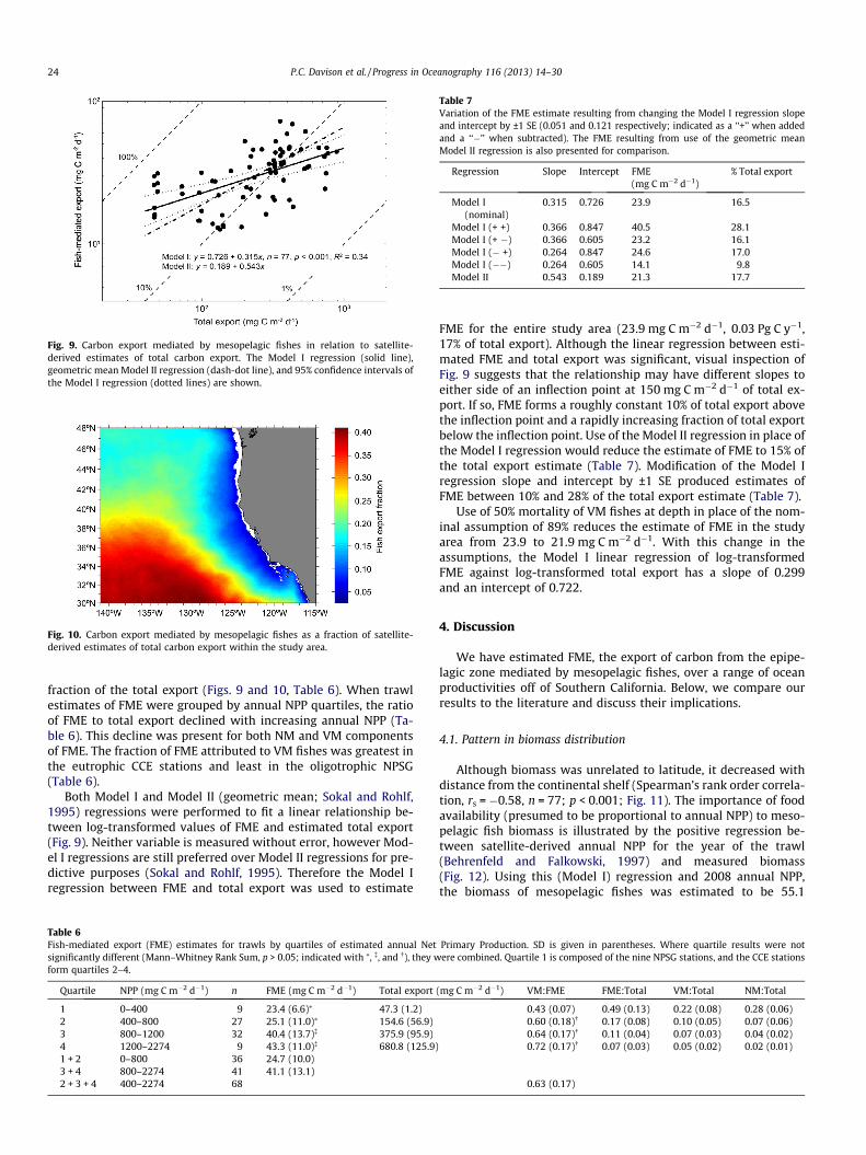
Fig. 9. Carbon export mediated by mesopelagic fishes in relation to satellite-derived estimates of total carbon export. The Model I regression (solid line),geometric mean Model II regression (dash-dot line), and 95% confidence intervals ofthe Model I regression (dotted lines) are shown.

Fig. 10. Carbon export mediated by mesopelagic fishes as a fraction of satellite-derived estimates of total carbon export within the study area.

Table 7Variation of the FME estimate resulting from changing the Model I regression slopeand intercept by ±1 SE (0.051 and 0.121 respectively; indicated as a ‘‘+’’ when addedand a ‘‘�’’ when subtracted). The FME resulting from use of the geometric meanModel II regression is also presented for comparison.

Regression Slope Intercept FME(mg C m�2 d�1)

% Total export

Model I(nominal)

0.315 0.726 23.9 16.5

Model I (+ +) 0.366 0.847 40.5 28.1Model I (+ �) 0.366 0.605 23.2 16.1Model I (� +) 0.264 0.847 24.6 17.0Model I (��) 0.264 0.605 14.1 9.8Model II 0.543 0.189 21.3 17.7


fraction of the total export (Figs. 9 and 10, Table 6). When trawlestimates of FME were grouped by annual NPP quartiles, the ratioof FME to total export declined with increasing annual NPP (Ta-ble 6). This decline was present for both NM and VM componentsof FME. The fraction of FME attributed to VM fishes was greatest inthe eutrophic CCE stations and least in the oligotrophic NPSG(Table 6).

Both Model I and Model II (geometric mean; Sokal and Rohlf,1995) regressions were performed to fit a linear relationship be-tween log-transformed values of FME and estimated total export(Fig. 9). Neither variable is measured without error, however Mod-el I regressions are still preferred over Model II regressions for pre-dictive purposes (Sokal and Rohlf, 1995). Therefore the Model Iregression between FME and total export was used to estimate

Table 6Fish-mediated export (FME) estimates for trawls by quartiles of estimated annual Netsignificantly different (Mann–Whitney Rank Sum, p > 0.05; indicated with ⁄, �, and �), they wform quartiles 2–4.

Quartile NPP (mg C m�2 d�1) n FME (mg C m�2 d�1) Total export

1 0–400 9 23.4 (6.6)⁄ 47.3 (1.2)2 400–800 27 25.1 (11.0)⁄ 154.6 (56.9)3 800–1200 32 40.4 (13.7)� 375.9 (95.9)4 1200–2274 9 43.3 (11.0)� 680.8 (125.9)1 + 2 0–800 36 24.7 (10.0)3 + 4 800–2274 41 41.1 (13.1)2 + 3 + 4 400–2274 68

FME for the entire study area (23.9 mg C m�2 d�1, 0.03 Pg C y�1,17% of total export). Although the linear regression between esti-mated FME and total export was significant, visual inspection ofFig. 9 suggests that the relationship may have different slopes toeither side of an inflection point at 150 mg C m�2 d�1 of total ex-port. If so, FME forms a roughly constant 10% of total export abovethe inflection point and a rapidly increasing fraction of total exportbelow the inflection point. Use of the Model II regression in place ofthe Model I regression would reduce the estimate of FME to 15% ofthe total export estimate (Table 7). Modification of the Model Iregression slope and intercept by ±1 SE produced estimates ofFME between 10% and 28% of the total export estimate (Table 7).

Use of 50% mortality of VM fishes at depth in place of the nom-inal assumption of 89% reduces the estimate of FME in the studyarea from 23.9 to 21.9 mg C m�2 d�1. With this change in theassumptions, the Model I linear regression of log-transformedFME against log-transformed total export has a slope of 0.299and an intercept of 0.722.

4. Discussion

We have estimated FME, the export of carbon from the epipe-lagic zone mediated by mesopelagic fishes, over a range of oceanproductivities off of Southern California. Below, we compare ourresults to the literature and discuss their implications.

4.1. Pattern in biomass distribution

Although biomass was unrelated to latitude, it decreased withdistance from the continental shelf (Spearman’s rank order correla-tion, rs = �0.58, n = 77; p < 0.001; Fig. 11). The importance of foodavailability (presumed to be proportional to annual NPP) to meso-pelagic fish biomass is illustrated by the positive regression be-tween satellite-derived annual NPP for the year of the trawl(Behrenfeld and Falkowski, 1997) and measured biomass(Fig. 12). Using this (Model I) regression and 2008 annual NPP,the biomass of mesopelagic fishes was estimated to be 55.1

Primary Production. SD is given in parentheses. Where quartile results were notere combined. Quartile 1 is composed of the nine NPSG stations, and the CCE stations

(mg C m�2 d�1) VM:FME FME:Total VM:Total NM:Total

0.43 (0.07) 0.49 (0.13) 0.22 (0.08) 0.28 (0.06)0.60 (0.18)� 0.17 (0.08) 0.10 (0.05) 0.07 (0.06)0.64 (0.17)� 0.11 (0.04) 0.07 (0.03) 0.04 (0.02)0.72 (0.17)� 0.07 (0.03) 0.05 (0.02) 0.02 (0.01)

0.63 (0.17)

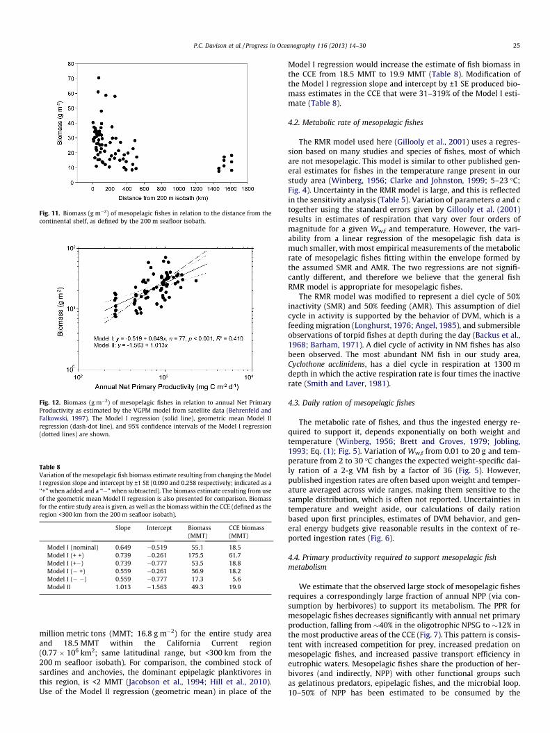
Fig. 11. Biomass (g m�2) of mesopelagic fishes in relation to the distance from thecontinental shelf, as defined by the 200 m seafloor isobath.

Fig. 12. Biomass (g m�2) of mesopelagic fishes in relation to annual Net PrimaryProductivity as estimated by the VGPM model from satellite data (Behrenfeld andFalkowski, 1997). The Model I regression (solid line), geometric mean Model IIregression (dash-dot line), and 95% confidence intervals of the Model I regression(dotted lines) are shown.

Table 8Variation of the mesopelagic fish biomass estimate resulting from changing the ModelI regression slope and intercept by ±1 SE (0.090 and 0.258 respectively; indicated as a‘‘+’’ when added and a ‘‘�’’ when subtracted). The biomass estimate resulting from useof the geometric mean Model II regression is also presented for comparison. Biomassfor the entire study area is given, as well as the biomass within the CCE (defined as theregion <300 km from the 200 m seafloor isobath).

Slope Intercept Biomass(MMT)

CCE biomass(MMT)

Model I (nominal) 0.649 �0.519 55.1 18.5Model I (+ +) 0.739 �0.261 175.5 61.7Model I (+�) 0.739 �0.777 53.5 18.8Model I (� +) 0.559 �0.261 56.9 18.2Model I (� �) 0.559 �0.777 17.3 5.6Model II 1.013 �1.563 49.3 19.9


million metric tons (MMT; 16.8 g m�2) for the entire study areaand 18.5 MMT within the California Current region(0.77 � 106 km2; same latitudinal range, but <300 km from the200 m seafloor isobath). For comparison, the combined stock ofsardines and anchovies, the dominant epipelagic planktivores inthis region, is <2 MMT (Jacobson et al., 1994; Hill et al., 2010).Use of the Model II regression (geometric mean) in place of the

Model I regression would increase the estimate of fish biomass inthe CCE from 18.5 MMT to 19.9 MMT (Table 8). Modification ofthe Model I regression slope and intercept by ±1 SE produced bio-mass estimates in the CCE that were 31–319% of the Model I esti-mate (Table 8).

4.2. Metabolic rate of mesopelagic fishes

The RMR model used here (Gillooly et al., 2001) uses a regres-sion based on many studies and species of fishes, most of whichare not mesopelagic. This model is similar to other published gen-eral estimates for fishes in the temperature range present in ourstudy area (Winberg, 1956; Clarke and Johnston, 1999; 5–23 �C;Fig. 4). Uncertainty in the RMR model is large, and this is reflectedin the sensitivity analysis (Table 5). Variation of parameters a and ctogether using the standard errors given by Gillooly et al. (2001)results in estimates of respiration that vary over four orders ofmagnitude for a given Ww,f and temperature. However, the vari-ability from a linear regression of the mesopelagic fish data ismuch smaller, with most empirical measurements of the metabolicrate of mesopelagic fishes fitting within the envelope formed bythe assumed SMR and AMR. The two regressions are not signifi-cantly different, and therefore we believe that the general fishRMR model is appropriate for mesopelagic fishes.

The RMR model was modified to represent a diel cycle of 50%inactivity (SMR) and 50% feeding (AMR). This assumption of dielcycle in activity is supported by the behavior of DVM, which is afeeding migration (Longhurst, 1976; Angel, 1985), and submersibleobservations of torpid fishes at depth during the day (Backus et al.,1968; Barham, 1971). A diel cycle of activity in NM fishes has alsobeen observed. The most abundant NM fish in our study area,Cyclothone acclinidens, has a diel cycle in respiration at 1300 mdepth in which the active respiration rate is four times the inactiverate (Smith and Laver, 1981).

4.3. Daily ration of mesopelagic fishes

The metabolic rate of fishes, and thus the ingested energy re-quired to support it, depends exponentially on both weight andtemperature (Winberg, 1956; Brett and Groves, 1979; Jobling,1993; Eq. (1); Fig. 5). Variation of Ww,f from 0.01 to 20 g and tem-perature from 2 to 30 �C changes the expected weight-specific dai-ly ration of a 2-g VM fish by a factor of 36 (Fig. 5). However,published ingestion rates are often based upon weight and temper-ature averaged across wide ranges, making them sensitive to thesample distribution, which is often not reported. Uncertainties intemperature and weight aside, our calculations of daily rationbased upon first principles, estimates of DVM behavior, and gen-eral energy budgets give reasonable results in the context of re-ported ingestion rates (Fig. 6).

4.4. Primary productivity required to support mesopelagic fishmetabolism

We estimate that the observed large stock of mesopelagic fishesrequires a correspondingly large fraction of annual NPP (via con-sumption by herbivores) to support its metabolism. The PPR formesopelagic fishes decreases significantly with annual net primaryproduction, falling from �40% in the oligotrophic NPSG to �12% inthe most productive areas of the CCE (Fig. 7). This pattern is consis-tent with increased competition for prey, increased predation onmesopelagic fishes, and increased passive transport efficiency ineutrophic waters. Mesopelagic fishes share the production of her-bivores (and indirectly, NPP) with other functional groups suchas gelatinous predators, epipelagic fishes, and the microbial loop.10–50% of NPP has been estimated to be consumed by the


microbial loop alone (Azam et al., 1983), and is not available tomesopelagic fishes. Possible confounding factors to the PPR esti-mate include an increase in capture efficiency offshore (fishes tendto be smaller offshore, and perhaps less able to avoid the net), tro-phic efficiency uncertainty, possible variation in trophic efficiencybetween the NPSG and the CCE, a reduction in trophic level ofmesopelagic fishes in the NPSG, and underestimation of annualNPP by the VGPM model.

Compound-specific isotope analysis (CSIA) indicates that myc-tophids in the NPSG may feed at a slightly lower trophic level thanthose in the CCE. Trophic level is �3.2 based upon stomach con-tents, but �2.9 based upon CSIA for myctophids from the NPSGand CCE respectively (Choy et al., 2012). A reduction of trophic le-vel below 3.0 (our assumed value was 3.2 for both the NPSG andCCE) requires some herbivory. This has only been observed oncein mesopelagic fishes (Robison, 1984), but it was for Ceratoscopeluswarmingii, one of the dominant myctophid species of the NPSG.

Trophic (or ecologic) efficiency has been estimated to be 10–20% for marine ecosystems (Peterson and Wroblewski, 1984; Paulyand Christensen, 1995; Lalli and Parsons, 1997), and has a maximalpossible value equivalent to the gross growth efficiency (GGE; G/I).GGE has been estimated to be 16–42% for marine poikilotherms(Brett and Groves, 1979; Childress et al., 1980; Ross, 1982; Jobling,1994; Harris et al., 2000). The difference between trophic efficiencyand GGE is production consumed by the microbial loop or ex-ported. Approximately 90% of the sediment sinking through themesopelagic (150–1000 m depth) is consumed there (Martinet al., 1987). Thus, if the consumption by microbial and detritalfood webs is explicitly considered, GGE (�30%) is perhaps a betterefficiency to use, whereas lower efficiencies are more appropriatewhen detrital and microbial losses are not quantified (�10%). Thus,we use an intermediate value of trophic efficiency for PPR calcula-tion and present results for a 10–30% range (Fig. 7). Previous at-tempts to reconcile the productivity of subtropical mesopelagicfishes with NPP have concluded that there is not enough NPP tosupport them if trophic level is >3 and trophic transfer efficiencyis 10% (Clarke, 1973; Mann, 1984). It has also been found that iftrophic efficiency is less than 13% there is not enough NPP in thewestern subarctic Pacific to support Neocalanus spp., copepods thatare important prey of mesopelagic fishes (Kobari et al., 2003). Ourdata are not consistent with 10% trophic efficiency in the NPSG, be-cause if true, �90% of NPP would be required to support the herbi-vores consumed by mesopelagic fishes.

Recent evidence suggests that global gross primary productionhas been underestimated (Welp et al., 2011; but the authors attri-bute it to terrestrial sources), and that nitrogen fixation at depthsbelow those observed by satellites plays a larger role in the oligo-trophic eastern North Pacific than previously believed (Montoyaet al., 2004), supporting the possibility that NPP is underestimatedhere. Satellite measurements of surface ocean color can be poorpredictor of integrated NPP in the NPSG (Letelier and Karl, 1996;Falkowski et al., 2003). Reconciliation of these diverse fields ofecology will require more research.

4.5. Cost of DVM

We found that approximately half of the taxonomically deter-mined VM biomass remains below 150 m during the night (Bs:-Bvm = 54.1%). The reasons for this are unknown, but may berelated to foraging success and predation risk. Vertical migrationwas estimated to comprise 67% of the total daily energy budgetof a VM fish. Looked at another way, if a VM fish can meet 60%of its normal daily energy requirement at depth, or if it consumed160% of Rd the previous night in the epipelagic, it would not needto ascend to the surface to feed. Non-migration may be advanta-geous to a fish if vertical migration elevates predation risk, either

in transit or at the surface. There is evidence of partial populationmigration and feeding at depth by VM fishes that supports condi-tional vertical migration (Pearcy et al., 1977, 1979; Gorbatenko andIl’inskii, 1991). It remains unclear whether or not VM fishes make adaily decision to migrate based upon hunger.

4.6. Carbon export

Annual NPP, exported production as a fraction of NPP (ef ratio;Laws et al., 2000), total carbon export, and estimated FME all hadsimilar areal patterns, i.e., high in the coastal upwelling zone,low in the NPSG, and moderate offshore from 40 to 48�N in theNorth Pacific Current (Fig. 8). However, the ratio of FME to total ex-port had an inverted pattern in relation to those ecological quanti-ties (Fig. 10). This inverted pattern occurs because the rationumerator (FME, proportional to biomass) is a function of NPP,whereas the denominator (total export, ef ratio times NPP) is afunction of the square of NPP. The occurrence of relatively highFME in subtropical regions (Fig. 3) is important because these oli-gotrophic waters form �60% of overall ocean area and are the siteof approximately half of oceanic carbon export (Emerson et al.,1997). FME is likely to be high in ocean regions that have warmwater at mesopelagic depths due to elevated metabolic rates, butno such conditions were present in our study area.

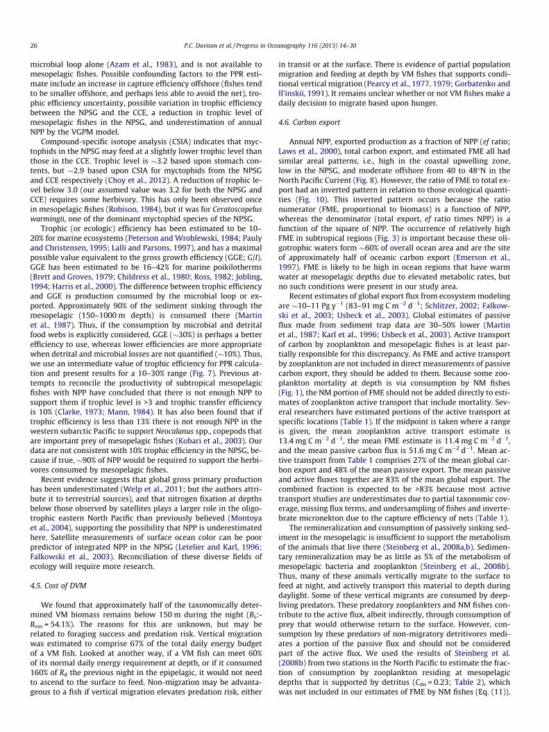
Recent estimates of global export flux from ecosystem modelingare �10–11 Pg y�1 (83–91 mg C m�2 d�1; Schlitzer, 2002; Falkow-ski et al., 2003; Usbeck et al., 2003). Global estimates of passiveflux made from sediment trap data are 30–50% lower (Martinet al., 1987; Karl et al., 1996; Usbeck et al., 2003). Active transportof carbon by zooplankton and mesopelagic fishes is at least par-tially responsible for this discrepancy. As FME and active transportby zooplankton are not included in direct measurements of passivecarbon export, they should be added to them. Because some zoo-plankton mortality at depth is via consumption by NM fishes(Fig. 1), the NM portion of FME should not be added directly to esti-mates of zooplankton active transport that include mortality. Sev-eral researchers have estimated portions of the active transport atspecific locations (Table 1). If the midpoint is taken where a rangeis given, the mean zooplankton active transport estimate is13.4 mg C m�2 d�1, the mean FME estimate is 11.4 mg C m�2 d�1,and the mean passive carbon flux is 51.6 mg C m�2 d�1. Mean ac-tive transport from Table 1 comprises 27% of the mean global car-bon export and 48% of the mean passive export. The mean passiveand active fluxes together are 83% of the mean global export. Thecombined fraction is expected to be >83% because most activetransport studies are underestimates due to partial taxonomic cov-erage, missing flux terms, and undersampling of fishes and inverte-brate micronekton due to the capture efficiency of nets (Table 1).

The remineralization and consumption of passively sinking sed-iment in the mesopelagic is insufficient to support the metabolismof the animals that live there (Steinberg et al., 2008a,b). Sedimen-tary remineralization may be as little as 5% of the metabolism ofmesopelagic bacteria and zooplankton (Steinberg et al., 2008b).Thus, many of these animals vertically migrate to the surface tofeed at night, and actively transport this material to depth duringdaylight. Some of these vertical migrants are consumed by deep-living predators. These predatory zooplankters and NM fishes con-tribute to the active flux, albeit indirectly, through consumption ofprey that would otherwise return to the surface. However, con-sumption by these predators of non-migratory detritivores medi-ates a portion of the passive flux and should not be consideredpart of the active flux. We used the results of Steinberg et al.(2008b) from two stations in the North Pacific to estimate the frac-tion of consumption by zooplankton residing at mesopelagicdepths that is supported by detritus (Cdo = 0.23; Table 2), whichwas not included in our estimates of FME by NM fishes (Eq. (11)).


NM export is 43% of FME in the NPSG, and 63% in the CCE (Ta-ble 6). This difference is likely due to the larger fraction of VM fishbiomass in the CCE compared to the NPSG (26% and 15% of totalbiomass respectively). Thus, vertical migration of fishes is less pre-valent and less important to active transport in the oligotrophicNPSG than it is in the more productive CCE. A possible explanationfor this pattern may be greater foraging success of fishes at depthand/or greater near-surface predation risk at night in the moretransparent waters of the NPSG. A similar pattern was observedby Steinberg et al. (2008a) for vertically migratory zooplankton(Table 1), in which the more productive station (K2) had a higherincidence of DVM and more efficient active transport by zooplank-ton than was observed at the oligotrophic station (ALOHA).

4.7. Sources of error

Singly varying the FME model parameters (excluding those formetabolic rate) resulted in an individual carbon flux range of0.76–1.43 times that predicted from the nominal values (Table 5).Error in respiration rate has a much stronger effect on estimates ofFME, however mesopelagic fishes do not differ from a general rela-tionship developed for fishes (Gillooly et al., 2001), and the nomi-nal values of metabolic model and respiration rate parametersproduce estimates of Rd for individual fishes that are consistentwith empirical measurements (Fig. 6).

There are few estimates of the consumption of VM fishes bydeep-living piscivores. The fraction of mesopelagic fish productionconsumed by deep-living piscivores (or its complement, consump-tion by epipelagic piscivores) is unknown in our study area. We usea nominal assumption of 89% mortality at depth from dragonfishesfrom the Gulf of Mexico (Sutton and Hopkins, 1996). This has alsobeen estimated to be 95% (Hopkins et al., 1996) and 58–230%(Clarke, 1982). Aggregated bottom-associated predators may con-sume so much VM fish production that they rely on advection ofthe DSL to support their metabolism (Koslow, 1996). This is consis-tent with studies showing that mesopelagic fish production is lar-gely isolated from epipelagic piscivores (Roger and Grandperrin,1976; Mann, 1984). Nevertheless, many epipelagic predators feedon mesopelagic fishes, and some piscivores predominantly con-sume them. By difference, this predation rate is assumed to be11% here. Studies of the consumption by individual piscivorousspecies inhabiting our study area are consistent with this whencompared to our biomass estimates (mesopelagic fishes comprise<5% of albacore diet, Glaser, 2010; 2% of the standing stock ofmesopelagic fishes are consumed annually by cetaceans in theCCE, Barlow et al., 2008; 2–8% of the standing stock of myctophidsare consumed annually by neon flying squid in the North Pacifictransition zone, Watanabe et al., 2004). However, because thesum of predation by epipelagic piscivores is unknown, as is thecomplementary consumption by deep-living piscivores, the frac-tion of VM fish mortality at depth is better expressed as a range.We used a conservative estimate of stomiid predation (50%) nearthe low estimate of Clarke (1982; 58%) with our FME model toput a lower bound on our estimate of FME due to reasonable var-iation in this parameter. Thus, we estimate FME to be 21.9–23.9 mg C m�2 d�1 in the study area. The use of 50% mortality atdepth in place of 89% decreases our estimate of FME by 8%. Mortal-ity rate at depth was also varied as part of the sensitivity analysis,and this decreased FME by only 11% under the conditions de-scribed in Table 5. Large variation in this parameter has little effecton the results of our study, or to our overall conclusions.

Error in the capture efficiency estimate for the MOHT and IKMT(14% and 6.6% respectively) will have a multiplicative impact onestimated FME. Our capture efficiency estimates for mesopelagicfishes are consistent with published estimates for similar nets(Barkley, 1972; Baird et al., 1974; Kaartvedt et al., 2012), and the

2.1-fold difference in capture efficiency between the IKMT andMOHT is almost identical to the difference reported by Yamamuraet al. (2010) for the same net designs and age-0 walleye pollock.

It is known that trawl-based estimates of the biomass of meso-pelagic micronekton biomass are highly variable, with the catchfrom repeated trawls varying by a factor of two from the mean (At-satt and Seapy, 1974; Angel and Baker, 1982). Our biomass esti-mates were consistent with this finding in the CCE (withoccasional very large catches), but less variable in the NPSG(Fig. 11). The reduction in biomass variability with distance off-shore suggests that mesoscale habitat patchiness may contributemore error to trawl-based biomass estimates than smaller-scalepatchiness in abundance does, although community differencescannot be excluded. Our sampling was appropriate for the studyregion, with 68 stations in the highly variable CCE waters, and 9stations in the less-variable NPSG (Fig. 2).

Variation in the denominator (total export) may affect our esti-mate of the relative importance of FME. We use the VGPM (Behren-feld and Falkowski, 1997) model to estimate NPP and the Laws(2004) model to estimate total export. The VGPM has been shownto overestimate NPP in the CCE (Kahru et al., 2009). An overesti-mate of NPP produces an overestimate of ef ratio by the Laws(2004) model, and thus an overestimate of total export. In theNPSG, the combination of the Laws (2004) and VGPM models hasbeen shown to produce a total export that is consistent with air-sea CO2 flux (Takahashi et al., 2002). The ratio of FME to total ex-port is then expected to be biased low in the CCE and unbiasedin the NPSG.

A Model I regression of the estimated FME to estimated total ex-port at the sampling stations was used to estimate FME for the en-tire study area (Fig. 10). The use of the geometric mean Model IIregression produces a similar regional FME estimate to the ModelI regression (Table 7), but it de-emphasizes the observed differencein FME between the NPSG and CCE and poorly fits the data fromthe NPSG stations (Fig. 9). Variation of the Model I regression slopeand intercept by ±1 SE produced FME estimates 59–170% of thenominal estimate (Table 7).

There are many sources of stochastic variation and potential er-ror in the estimate of FME presented here. However, unless errorsin parameter estimation, total export, and the regression of FME ontotal export are systematically biased, they are not likely to greatlychange our overall conclusion that FME is an appreciable fractionof total export in the study area.

4.8. Vertical distribution of exported carbon

The respiratory fraction of overall FME will be to shallow depths(150–400 m) with moderate ventilation times. Most of the respiredcarbon will be at the daytime depth of the DSL (400 m here), as res-piration during vertical movement is small in comparison the total(Table 4). The fecal fraction will be exported quickly to greaterdepths (mesopelagic fish feces sink at �1000 m d�1; Robison andBailey, 1981), and may be sequestered from the atmosphere on atime scale of centuries. Although not counted as export here, Cdo

is repackaged as rapidly sinking feces by NM fishes. NM fishes thusplay a role in the transformation of slowly sinking detritus atmesopelagic depths to fast-sinking detritus that may reach thesea floor. The fate of the mortality export term is predator-specific.Given the assumption that 89% of mesopelagic zooplanktivore pro-duction is consumed by dragonfishes (Sutton and Hopkins, 1996),it is likely that carbon lost to mortality will be transformed at asimilar depth and in similar ratios as the forage of NM fishes(42% respired, 18% defecated, and 40% passed on to the next pred-ator). Thus, most FME is to depths of 400 m or more. Conversely, asmuch as 80% of the passive flux is remineralized between 150 and

Table 9Comparison of total carbon export (2008; Laws, 2004), passive flux from sediment traps (150 m; 400 m; Martin et al., 1987), and fish-mediated export (FME) at the four VERTEXsediment trap stations in the study area (Fig. 8c). ‘‘VM’’ refers to the estimated FME contributed by VM fishes (Table 6).

PREVTX 37.0�N, 123.0�W(mg C m�2 d�1)

Station 1 36.1�N, 122.6�W(mg C m�2 d�1)

Station 2 35.0�N, 128.2�W(mg C m�2 d�1)

Station 4 33.3�N, 139.2�W(mg C m�2 d�1)

Total export 666.1 557.0 80.7 47.0Sed. trap (150 m) 80.4 166.0 54.6 45.5Sed. trap (400 m) 34.5 73.4 23.1 17.6FME 42.8 40.5 22.0 18.6VM 30.8 25.9 9.5 8.0


500 m (Buesseler et al., 2007b). At a depth of 400 m, FME is approx-imately equal to the passive flux (Table 9).

5. Conclusions

Quantifying the efficiency of the biological pump is a prerequi-site for forming accurate global carbon models (Usbeck et al.,2003). Few studies of the biological pump to date have quantifiedthe role of mesopelagic fishes in the export of carbon from the epi-pelagic. Our results indicate that not only is the FME large in com-parison to mean zooplankton flux estimates (Table 1), but that it isapproximately equal to the passive flux at 400 m depth (Table 9),and that it varies spatially in both magnitude and relative impor-tance (Figs. 9 and 10). The size, swimming ability, and abundanceof mesopelagic fishes serve to elevate their importance to the bio-logical pump. Their feces sink rapidly, and they are isolated fromepipelagic predators. Their daily vertical movements, or those oftheir prey, take them through the upper thermocline, and they re-lease carbon in the form of defecation, respiration, and mortalitybelow the depth zone in which most remineralization occurs.Mesopelagic fishes require a greater proportion of NPP in the oligo-trophic NPSG than in the more productive CCE (Fig. 7). We esti-mate that mesopelagic fishes mediate a mean of 15–17% (21.9–23.9 mg C m�2 d�1) of the total carbon export in the study area.Approximately half of this export passes through VM fishes ofWw,f > 1 g (Fig. 3), over 90% of which are myctophids (Table 3).The magnitude of FME is estimated to exceed 40% of the total ex-port in the oligotrophic NPSG, where remineralization of passivecarbon flux is most efficient (Figs. 9 and 10). FME is larger in pro-ductive coastal upwelling areas, but forms a smaller fraction of thetotal export (Fig. 9). VM fishes contribute a smaller fraction (43%)to FME in the NPSG than in the more productive CCE (63%; Table 6).FME is likely to be high in ocean regions that have warm water atmesopelagic depths due to elevated metabolic rates, but no suchconditions were present in our study area. As FME largely bypassesdirect measurements of passive carbon export, it is additive to esti-mates of the biological pump made with them. This often-neglected component of the biological pump is large enough toaffect global biogeochemical models that are currently fit to sedi-ment trap data.

Acknowledgements

Funding for the MOHT was provided by the Moore Foundation.P. Davison was supported by a NASA Earth and Space Science Fel-lowship. Funding for the SEAPLEX cruise was provided by Univer-sity of California Ship Funds, Project Kaisei/Ocean VoyagesInstitute, and NSF IGERT Grant #0333444. Wire time for midwatertrawling was provided by the California Current Ecosystem LTERsite, supported by NSF, and by NOAA. Chemicals, equipment, andlaboratory space were provided by the SIO Marine Vertebrateand Pelagic Invertebrate Collections. The authors thank the cap-tains, crews, and science parties of the R/V Melville, R/V New Hori-zon, and NOAA Ship McArthur II for assistance deploying the trawls

and processing the samples. G. Watters, A. Henry, and D. Griffithprovided gear and assistance for the ORCAWALE cruise. A. Suntsovperformed�40% of the ORCAWALE IKMT trawls. J. Cox, I. Ionescu, J.Blackburn, S. Lyday, and L. Carswell assisted with ORCAWALE IKMTtrawling. C. Klepadlo from the Scripps Institution of OceanographyMarine Vertebrate Collection helped with the identification ofmesopelagic fishes. R. Raymond provided assistance processingsome of the samples. J. Liu and A. Lara-Lopez assisted the CCE-LTERMOHT trawling. A. Netburn provided helpful feedback on themanuscript.

Appendix A. Supplementary material

Supplementary data associated with this article can be found inthe online version, at http://dx.doi.org/10.1016/j.pocean.2013.05.013.

References

Alexander, R.M., 2003. Principles of Animal Locomotion. Princeton University Press,Princeton.

Al-Mutairi, H., Landry, M.R., 2001. Active export of carbon and nitrogen at StationALOHA by diel migrant zooplankton. Deep-Sea Research Part II 48, 2083–2103.

Angel, M.V., 1985. Vertical migrations in the oceanic realm: possible causes andprobable effects. In M.A. Rankin (Ed.), Migration: Mechanisms and adaptivesignificance, Contributions in Marine Science, 27 (Supplement) (pp. 45–70).Port Aransas: Marine Science Institute.

Angel, M.V., 1989a. Does mesopelagic biology affect the vertical flux? In: Berger,W.H., Smetacek, V.S., Wefer, G. (Eds.), Productivity of the Ocean: Present andPast. John Wiley & Sons Limited, New York, pp. 155–173.

Angel, M.V., 1989b. Vertical profiles of pelagic communities in the vicinity of theAzores Front and their implications to deep ocean ecology. Progress inOceanography 22, 1–46.

Angel, M.V., Baker, A.d.C., 1982. Vertical distribution of the standing crop ofplankton and micronekton at three stations in the Northeast Atlantic. BiologicalOceanography 2, 1.

Angel, M.V., Pugh, P.R., 2000. Quantification of diel vertical migration bymicronektonic taxa in the northeast Atlantic. Hydrobiologia 440, 161–179.

Atsatt, L.H., Seapy, R.R., 1974. Analysis of sampling variability in replicatedmidwater trawls off southern-California. Journal of Experimental MarineBiology and Ecology 14, 261–273.

Azam, F., Fenchel, T., Field, J.G., Gray, J.S., Meyerreil, L.A., Thingstad, F., 1983. Theecological role of water-column microbes in the sea. Marine Ecology ProgressSeries 10, 257–263.

Backus, R.H., Craddock, J.E., Haedrich, R.L., Shores, D.L., Teal, J.M., Wing, A.S., Mead,G.W., Clarke, W.D., 1968. Ceratoscopelus maderensis: peculiar sound-scatteringlayer identified with this myctophid fish. Science 160, 991–993.

Bailey, T.G., Robison, B.H., 1986. Food availability as a selective factor on thechemical compositions of midwater fishes in the eastern North Pacific. MarineBiology 91, 131–141.

Baird, R.C., 1971. The systematics, distribution, and zoogeography of the marinehatchetfishes (family Sternoptychidae). Bulletin of the Museum of ComparativeZoology 142, 1–128.

Baird, R.C., Wilson, D.F., Beckett, R.C., Hopkins, T.L., 1974. Diaphus taaningi Norman,principal component of a shallow sound-scattering layer in the Cariaco Trench,Venezuela. Journal of Marine Research 32, 301–312.

Barham, E.G., 1971. Deep-sea fishes: lethargy and vertical orientation. In: Farquhar,G.B. (Ed.), Proceedings of an International Symposium on Biological SoundScattering in the Ocean. Maury Center for Ocean Science Report 005. U.S.Government Printing Office, Washington, DC, pp. 100–118.

Barkley, R.A., 1972. Selectivity of towed-net samplers. Fishery Bulletin 70, 799–820.Barlow, J., Kahru, M., Mitchell, B.G., 2008. Cetacean biomass, prey consumption, and

primary production requirements in the California Current ecosystem. MarineEcology Progress Series 371, 285–295.



http://refhub.elsevier.com/S0079-6611(13)00055-4/h0010






































Behrenfeld, M.J., Falkowski, P.G., 1997. Photosynthetic rates derived from satellite-based chlorophyll concentration. Limnology and Oceanography 42, 1–20.

Benoit-Bird, K.J., Au, W.W.L., 2006. Extreme diel horizontal migrations by a tropicalnearshore resident micronekton community. Marine Ecology Progress Series319, 1–14.

Borodulina, O.D., 1972. The feeding of mesopelagic predatory fish in the open ocean.Journal of Ichthyology 12, 692–703.

Bradford-Grieve, J.M., Nodder, S.D., Jillett, J.B., Currie, K., Lassey, K.R., 2001. Potentialcontribution that the copepod Neocalanus tonsus makes to downward carbonflux in the Southern Ocean. Journal of Plankton Research 23, 963–975.

Brett, J.R., Groves, T.D.D., 1979. Physiological energetics. In: Hoar, W.S., Randall, D.J.(Eds.), Bioenergetics and Growth, vol. 8. Academic Press, New York, pp. 279–351.

Buesseler, K.O., Boyd, P.W., 2009. Shedding light on processes that control particleexport and flux attenuation in the twilight zone of the open ocean. Limnologyand Oceanography 54, 1210–1232.

Buesseler, K.O., Antia, A.N., Chen, M., Fowler, S.W., Gardner, W.D., Gustafsson, O.,Harada, K., Michaels, A.F., van der Loeff, M.R., Sarin, M., Steinberg, D.K., Trull, T.,2007a. An assessment of the use of sediment traps for estimating upper oceanparticle fluxes. Journal of Marine Research 65, 345–416.

Buesseler, K.O., Lamborg, C.H., Boyd, P.W., Lam, P.J., Trull, T.W., Bidigare, R.R.,Bishop, J.K.B., Casciotti, K.L., Dehairs, F., Elskens, M., Honda, M., Karl, D.M., Siegel,D.A., Silver, M.W., Steinberg, D.K., Valdes, J., Van Mooy, B., Wilson, S., 2007b.Revisiting carbon flux through the ocean’s twilight zone. Science 316, 567–570.

Childress, J.J., Nygaard, M.H., 1973. Chemical composition of midwater fishes as afunction of depth of occurrence off southern California. Deep-Sea Research 20,1093–1109.

Childress, J.J., Nygaard, M., 1974. Chemical composition and buoyancy of midwatercrustaceans as function of depth of occurrence off southern California. MarineBiology 27, 225–238.

Childress, J.J., Somero, G.N., 1979. Depth-related enzymic activities in muscle, brainand heart of deep-living pelagic marine teleosts. Marine Biology 52, 273–283.

Childress, J.J., Taylor, S.M., Cailliet, G.M., Price, M.H., 1980. Patterns of growth,energy utilization and reproduction in some meso- and bathypelagic fishes offsouthern California. Marine Biology 61, 27–40.

Choy, A.C., Davison, P.C., Drazen, J.C., Flynn, A., Gier, E.J., Hoffman, J.C., McClain-Counts, J.P., Miller, T.W., Popp, B.N., Ross, S.W., Sutton, T.T., 2012. Global trophicposition comparison of two dominant mesopelagic fish families (Myctophidae,Stomiidae) using amino acid nitrogen isotopic analyses. Plos One 7, 1–8.

Clarke, W.D., 1971. Comparison of different investigative techniques for studyingthe deep scattering layers. In: Farquhar, G.B. (Ed.), Proceedings of anInternational Symposium on Biological Sound Scattering in the Ocean. MauryCenter for Ocean Sciences Report 005. U.S. Government Printing Office,Washington, DC, pp. 550–562.

Clarke, T.A., 1973. Some aspects of the ecology of lanternfishes (Myctophidae) in thePacific Ocean near Hawaii. Fishery Bulletin 71, 401–434.

Clarke, T.A., 1978. Diel feeding patterns of 16 species of mesopelagic fishes fromHawaiian waters. Fishery Bulletin 76, 495–513.

Clarke, T.A., 1982. Feeding habits of stomiatoid fishes from Hawaiian waters.Fishery Bulletin 80, 287–304.

Clarke, A., Johnston, N.M., 1999. Scaling of metabolic rate with body mass andtemperature in teleost fish. Journal of Animal Ecology 68, 893–905.

Dalpadado, P., Gjosaeter, J., 1988. Feeding ecology of the lanternfish Benthosemapterotum from the Indian Ocean. Marine Biology 99, 555–567.

Dam, H.G., Roman, M.R., Youngbluth, M.J., 1995. Downward export of respiratorycarbon and dissolved inorganic nitrogen by diel-migrant mesozooplankton atthe JGOFS Bermuda time-series station. Deep-Sea Research 42, 1187–1197.

Davison, P., 2011. The Export of Carbon Mediated by Mesopelagic Fishes in theNortheast Pacific Ocean. PhD Thesis, University of California, San Diego.

Denman, K.L., Brasseur, G., Chidthaisong, A., Ciais, P., Cox, P.M., Dickinson, R.E.,Hauglustaine, D., Heinze, C., Holland, E., Jacob, D., Lohmann, U., Ramachandran,S., da Silva Dias, P.L., Wofsy, S.C., Zhang, X., 2007. Couplings between changes inthe climate system and biogeochemistry. In: Solomon, S., Qin, D., Manning, M.,Chen, Z., Marquis, M., Averyt, K.B., Tignor, M., Miller, H.L. (Eds.), Climate Change2007: The Physical Science Basis. Cambridge University Press, New York, pp.499–587.

Donnelly, J., Torres, J.J., 1988. Oxygen consumption of midwater fishes andcrustaceans from the eastern Gulf of Mexico. Marine Biology 97, 483–494.

Emerson, S., Quay, P., Karl, D., Winn, C., Tupas, L., Landry, M., 1997. Experimentaldetermination of the organic carbon flux from open-ocean surface waters.Nature 389, 951–954.

Falkowski, P.G., Laws, E.A., Barber, R.T., Murray, J.W., 2003. Phytoplankton and theirrole in primary, new, and export production. In: Fasham, M.J.R. (Ed.), OceanBiogeochemistry. Springer-Verlag, Berlin, pp. 99–121.

Fowler, S.W., Knauer, G.A., 1986. Role of large particles in the transport of elementsand organic compounds through the oceanic water column. Progress inOceanography 16, 147–194.

Gerasimova, O., 1990. Feeding and food intake of Electrona carlsbergi (Taning, 1932)Myctophidae. Selected Science Paper CCAMLR 7, 411–416.

Gillooly, J.F., Brown, J.H., West, G.B., Savage, V.M., Charnov, E.L., 2001. Effects of sizeand temperature on metabolic rate. Science 293, 2248–2251.

Gjosaeter, J., Kawaguchi, K., 1980. A review of the world resources of mesopelagicfish. FAO Fisheries Technical Paper 193, 1–151.

Glaser, S.M., 2010. Interdecadal variability in predator–prey interactions of juvenileNorth Pacific albacore in the California Current System. Marine EcologyProgress Series 414, 209–221.

Gorbatenko, K.M., Il’inskii, E.N., 1991. Feeding behavior of the most commonmesopelagic fishes in the Bering Sea. Journal of Ichthyology 31, 816–821.

Gorelova, T.A., 1984. A quantitative assessment of consumption of zooplankton byepipelagic lanternfishes (family Myctophidae) in the equatorial Pacific Ocean.Journal of Ichthyology 23, 106–113.

Gorelova, T.A., Tseitlin, V.B., 1979. Feeding of mesopelagic fish of the genusCyclothone. Okeanologiya 19, 1110–1115.

Harris, R.P., Wiebe, P.H., Lenz, J., Skjoldal, H.R., Huntley, M., 2000. ZooplanktonMethodology Manual. Academic Press, London.

Hernandez-Leon, S., Gomez, M., Pagazaurtundua, M., Portillo-Hahnefeld, A.,Montero, I., Almeida, C., 2001. Vertical distribution of zooplankton in CanaryIsland waters: implications for export flux. Deep-Sea Research 48, 1071–1092.

Hickman, C.P., Trump, B.F., 1969. The kidney. In: Hoar, W.S., Randall, D.J. (Eds.), FishPhysiology, vol. 1. Academic Press, New York, pp. 91–239.

Hidaka, K., Kawaguchi, K., Murakami, M., Takahashi, M., 2001. Downward transportof organic carbon by diel migratory micronekton in the western equatorialPacific: its quantitative and qualitative importance. Deep-Sea Research 48,1923–1939.

Hill, K.T., Lo, N.C.H., Macewiz, B.J., Crone, P.R., Felix-Uraga, R., 2010. Assessment ofthe Pacific Sardine Resource in 2010 for U.S. Management in 2011. NOAATechnical Memorandum NMFS SWFSC-469, pp. 1–142.

Holton, A.A., 1969. Feeding behavior of a vertically migrating lanternfish. PacificScience 23, 325–331.

Hopkins, T.L., Baird, R.C., 1977. Aspects of the feeding ecology of oceanic midwaterfishes. In: Anderson, N.R., Zahuranec, B.J. (Eds.), Oceanic Sound ScatteringPrediction. Plenum Press, New York, pp. 325–360.

Hopkins, T.L., Baird, R.C., 1985. Feeding ecology of four hatchetfishes(Sternoptychidae) in the eastern Gulf of Mexico. Bulletin of Marine Science36, 260–277.

Hopkins, T.L., Sutton, T.T., Lancraft, T.M., 1996. The trophic structure and predationimpact of a low latitude midwater fish assemblage. Progress in Oceanography38, 205–239.

Ikeda, T., 1989. Estimated respiration rate of myctophid fish from the enzymeactivity of the electron-transport-system. Journal of the OceanographicalSociety of Japan 45, 167–173.

IPCC, 2007. Summary for policymakers. In: Solomon, S., Qin, D., Manning, M., Chen,Z., Marquis, M., Averyt, K.B., Tignor, M., Miller, H.L. (Eds.), Climate change 2007:The Physical Science Basis. Cambridge University Press, New York, pp. 1–18.

Isaacs, J.D., Kidd, L.W., 1953. Isaacs–Kidd midwater trawl final report. ScrippsInstitution of Oceanography Oceanographic Equipment Report 1, 1–21.

Jacobson, L.D., Lo, N.C.H., Barnes, J.T., 1994. A biomass-based assessment model fornorthern anchovy, Engraulis mordax. Fishery Bulletin 92, 711–724.

Jobling, M., 1993. Bioenergetics: feed intake and energy partitioning. In: Rankin, J.C.,Jensen, F.B. (Eds.), Fish Ecophysiology. Chapman and Hall, London, pp. 1–44.

Jobling, M., 1994. Fish Bioenergetics. Chapman and Hall, New York.Kaartvedt, S., Staby, A., Aksnes, D.L., 2012. Efficient trawl avoidance by mesopelagic

fishes causes large underestimation of their biomass. Marine Ecology ProgressSeries 456, 1–6.

Kahru, M., Kudela, R., Manzano-Sarabia, M., Mitchell, B.G., 2009. Trends in primaryproduction in the California Current detected with satellite data. Journal ofGeophysical Research, 114.

Karl, D.M., Christian, J.R., Dore, J.E., Hebel, D.V., Letelier, R.M., Tupas, L.M., Winn, C.D.,1996. Seasonal and interannual variability in primary production and particleflux at Station ALOHA. Deep-Sea Research Part II 43, 539–568.

Kobari, T., Shinada, A., Tsuda, A., 2003. Functional roles of interzonal migratingmesozooplankton in the western subarctic Pacific. Progress in Oceanography57, 279–298.

Kobari, T., Steinberg, D.K., Ueda, A., Tsuda, A., Silver, M.W., Kitamura, M., 2008.Impacts of ontogenetically migrating copepods on downward carbon flux in thewestern subarctic Pacific Ocean. Deep-Sea Research Part II 55, 1648–1660.

Koslow, J.A., 1996. Energetic and life-history patterns of deep-sea benthic,benthopelagic and seamount-associated fish. Journal of Fish Biology 49,54–74.

Koslow, J.A., Kloser, R.J., Williams, A., 1997. Pelagic biomass and communitystructure over the mid-continental slope off southeastern Australia based uponacoustic and midwater trawl sampling. Marine Ecology Progress Series 146, 21–35.

Lalli, C.M., Parsons, T.R., 1997. Biological Oceanography an Introduction.Butterworth-Heinemann, Oxford.

Laws, E., 2004. Export flux and stability as regulators of community composition inpelagic marine biological communities: implications for regime shifts. Progressin Oceanography 60, 343–354.

Laws, E.A., Falkowski, P.G., Smith, W.O., Ducklow, H., McCarthy, J.J., 2000.Temperature effects on export production in the open ocean. GlobalBiogeochemical Cycles 14, 1231–1246.

Le Borgne, R., Rodier, M., 1997. Net zooplankton and the biological pump: acomparison between the oligotrophic and mesotrophic equatorial Pacific. Deep-Sea Research Part II 44, 2003–2023.

Legand, M., Rivaton, J., 1969. Biological cycles of mesopelagic fishes of easternIndian Ocean 3: predatory activity of micronektonic fishes. Cahiers OrstomOceanographie 7, 29–45.

Letelier, R.M., Karl, D.M., 1996. Role of Trichodesmium spp. in the productivity of thesubtropical North Pacific Ocean. Marine Ecology Progress Series 133, 263–273.

Locarnini, R.A., Mishonov, A.V., Antonov, J.I., Boyer, T.P., Garcia, H.E., Baranova, H.A.,Zweng, M.M., Johnson, D.R., 2010. World Ocean Atlas 2009, vol. 1. Temperature.U.S. Government Printing Office, Washington, DC.




































































































































































Longhurst, A.R., 1976. Vertical migration. In: Cushing, D.H., Walsh, J.J. (Eds.), TheEcology of the Sea. Blackwell, Oxford, pp. 116–137.

Longhurst, A.R., Harrison, W.G., 1989. The biological pump: profiles of planktonproduction and consumption in the upper ocean. Progress in Oceanography 22,47–123.

Longhurst, A., Williams, R., 1992. Carbon flux by seasonal vertical migrant copepodsis a small number. Journal of Plankton Research 14, 1495–1509.

Longhurst, A.R., Bedo, A.W., Harrison, W.G., Head, E.J.H., Sameoto, D.D., 1990.Vertical flux of respiratory carbon by oceanic diel migrant biota. Deep-SeaResearch 37, 685–694.

Mann, K.H., 1984. Fish production in open ocean ecosystems. In: Fasham, M.J.R.(Ed.), Flows of Energy and Materials in Marine Ecosystems. Plenum Press, NewYork, pp. 435–458.

Martin, J.H., Knauer, G.A., Karl, D.M., Broenkow, W.W., 1987. VERTEX: carboncycling in the northeast Pacific. Deep-Sea Research 34, 267–285.

Martz, T.R., Johnson, K.S., Riser, S.C., 2008. Ocean metabolism observed with oxygensensors on profiling floats in the South Pacific. Limnology and Oceanography 53,2094–2111.

Montoya, J.P., Holl, C.M., Zehr, J.P., Hansen, A., Villareal, T.A., Capone, D.G., 2004.High rates of N2 fixation by unicellular diazotrophs in the oligotrophic PacificOcean. Nature 430, 1027–1031.

Morales, C.E., 1999. Carbon and nitrogen fluxes in the oceans: the contribution byzooplankton migrants to active transport in the North Atlantic during the JointGlobal Ocean Flux Study. Journal of Plankton Research 21, 1799–1808.

Morel, A., Berthon, J.F., 1989. Surface pigments, algal biomass profiles, and potentialproduction of the euphotic layer: relationships reinvestigated in view ofremote-sensing applications. Limnology and Oceanography 34, 1545–1562.

Oozeki, Y., Hu, F.X., Kubota, H., Sugisaki, H., Kimura, R., 2004. Newly designedquantitative frame trawl for sampling larval and juvenile pelagic fish. FisheriesScience 70, 223–232.

Pakhomov, E.A., Perissinotto, R., McQuaid, C.D., 1996. Prey composition and dailyrations of myctophid fishes in the Southern Ocean. Marine Ecology ProgressSeries 134, 1–14.

Pauly, D., Christensen, V., 1995. Primary production required to sustain globalfisheries. Nature 374, 255–257.

Pauly, D., Trites, A.W., Capuli, E., Christensen, V., 1998. Diet composition and trophiclevels of marine mammals. ICES Journal of Marine Science 55, 467–481.

Pearcy, W.G., 1964. Some distributional features of mesopelagic fishes off Oregon.Journal of Marine Research 22, 83–102.

Pearcy, W.G., Laurs, R.M., 1966. Vertical migration and distribution of mesopelagicfishes off Oregon. Deep-Sea Research 13, 153–165.

Pearcy, W.G., Krygier, E.E., Mesecar, R., Ramsey, F., 1977. Vertical distribution andmigration of oceanic micronekton off Oregon. Deep-Sea Research 24, 223–245.

Pearcy, W.G., Lorz, H.V., Peterson, W., 1979. Comparison of the feeding habits ofmigratory and non-migratory Stenobrachius leucopsarus (Myctophidae). MarineBiology 51, 1–8.

Pearre, S., 2003. Eat and run? The hunger/satiation hypothesis in vertical migration:history, evidence and consequences. Biological Reviews 78, 1–79.

Peterson, I., Wroblewski, J.S., 1984. Mortality rate of fishes in the pelagic ecosystem.Canadian Journal of Fisheries and Aquatic Sciences 41, 1117–1120.

Putzeys, S., Hernandez-Leon, S., 2005. A model of zooplankton diel verticalmigration off the Canary Islands: implication for active carbon flux. Journal ofSea Research 53, 213–222.

Radchenko, V.I., 2007. Mesopelagic fish community supplies ‘‘biological pump’’.Raffles Bulletin of Zoology, 265–271.

Robison, B.H., 1973. System for maintaining midwater fishes in captivity. Journal ofthe Fisheries Research Board of Canada 30, 126–128.

Robison, B.H., 1984. Herbivory by the myctophid fish Ceratoscopelus warmingii.Marine Biology 84, 119–123.

Robison, B.H., Bailey, T.G., 1981. Sinking rates and dissolution of midwater fish fecalmatter. Marine Biology 65, 135–142.

Roger, C., Grandperrin, R., 1976. Pelagic food webs in the tropical Pacific. Limnologyand Oceanography 21, 731–735.

Ross, R.M., 1982. Energetics of Euphausia pacifica. II. Complete carbon and nitrogenbudgets at 8 and 12 C throughout the life span. Marine Biology 68, 15–23.

Rowedder, U., 1979. Feeding ecology of the Myctophid Electrona antarctica(Gunther, 1878) (Teleostei). Meeresforschung – Reports on Marine Research27, 252–263.

Sameoto, D.D., 1988. Feeding of lantern fish Benthosema glaciale off the Nova Scotiashelf. Marine Ecology Progress Series 44, 113–129.

Sameoto, D., 1989. Feeding ecology of the lantern fish Benthosema glaciale in asubarctic region. Polar Biology 9, 169–178.

Schlitzer, R., 2002. Carbon export fluxes in the Southern Ocean: results from inversemodeling and comparison with satellite-based estimates. Deep-Sea ResearchPart II 49, 1623–1644.

Schnetzer, A., Steinberg, D.K., 2002. Active transport of particulate organic carbonand nitrogen by vertically migrating zooplankton in the Sargasso Sea. MarineEcology Progress Series 234, 71–84.

Silver, M.W., Coale, S.L., Pilskaln, C.H., Steinberg, D.R., 1998. Giant aggregates:importance as microbial centers and agents of material flux in the mesopelagiczone. Limnology and Oceanography 43, 498–507.

Smith, K.L., Laver, M.B., 1981. Respiration of the bathypelagic fish Cyclothoneacclinidens. Marine Biology 61, 261–266.

Sokal, R.R., Rohlf, F.J., 1995. Biometry. W. H. Freeman and Company, New York.Steinberg, D.K., Carlson, C.A., Bates, N.R., Goldthwait, S.A., Madin, L.P., Michaels, A.F.,

2000. Zooplankton vertical migration and the active transport of dissolvedorganic and inorganic carbon in the Sargasso Sea. Deep-Sea Research 47, 137–158.

Steinberg, D.K., Cope, J.S., Wilson, S.E., Kobari, T., 2008a. A comparison ofmesopelagic mesozooplankton community structure in the subtropical andsubarctic North Pacific Ocean. Deep-Sea Research Part II 55, 1615–1635.

Steinberg, D.K., Van Mooy, B.A.S., Buesseler, K.O., Boyd, P.W., Kobari, T., Karl, D.M.,2008b. Bacterial vs. zooplankton control of sinking particle flux in the ocean’stwilight zone. Limnology and Oceanography 53, 1327–1338.

Sutton, T.T., Hopkins, T.L., 1996. Trophic ecology of the stomiid (Pisces: Stomiidae)fish assemblage of the eastern Gulf of Mexico: Strategies, selectivity and impactof a top mesopelagic predator group. Marine Biology 127, 179–192.

Takahashi, T., Sutherland, S.C., Sweeney, C., Poisson, A., Metzl, N., Tilbrook, B., Bates,N., Wanninkhof, R., Feely, R.A., Sabine, C., Olafsson, J., Nojiri, Y., 2002. Globalsea–air CO2 flux based on climatological surface ocean pCO2, and seasonalbiological and temperature effects. Deep-Sea Research Part II 49, 1601–1622.

Takahashi, K., Kuwata, A., Sugisaki, H., Uchikawa, K., Saito, H., 2009. Downwardcarbon transport by diel vertical migration of the copepods Metridia pacifica andMetridia okhotensis in the Oyashio region of the western subarctic Pacific Ocean.Deep-Sea Research 56, 1777–1791.

Torres, J.J., Somero, G.N., 1988. Metabolism, enzymic activities and cold adaptationin Antarctic mesopelagic fishes. Marine Biology 98, 169–180.

Torres, J.J., Belman, B.W., Childress, J.J., 1979. Oxygen consumption rates ofmidwater fishes as a function of depth of occurrence. Deep-Sea Research 26,185–197.

Tseytlin, V.B., Gorelova, T.A., 1978. Studies of the feeding of the lanternfishMyctophum nitidulum (Myctophidae, Pisces). Oceanology 18, 488–492.

Usbeck, R., Schlitzer, R., Fischer, G., Wefer, G., 2003. Particle fluxes in the ocean:comparison of sediment trap data with results from inverse modeling. Journalof Marine Systems 39, 167–183.

Videler, J.J., 1993. Fish Swimming. Chapman and Hall, New York.Volk, T., Hoffert, M.I., 1985. Ocean carbon pumps: analysis of relative strengths and

efficiencies in ocean-driven atmospheric CO2 changes. In E. Sundquist, W.S.Broecker (Eds.), The carbon cycle and atmospheric CO2: natural variationsarchean to present. Geophysical Monograph, vol 32, American GeophysicalUnion.

Watanabe, H., Kawaguchi, K., 2003. Decadal change in the diets of the surfacemigratory myctophid fish Myctophum nitidulum in the Kuroshio region of thewestern North Pacific: predation on sardine larvae by myctophids. FisheriesScience 69, 716–721.

Watanabe, H., Kubodera, T., Ichii, T., Kawahara, S., 2004. Feeding habits of neonflying squid Ommastrephes bartramii in the transitional region of the centralNorth Pacific. Marine Ecology Progress Series 266, 173–184.

Watson, A.J., Orr, J.C., 2003. Carbon dioxide fluxes in the global ocean. In: Fasham,M.J.R. (Ed.), Ocean Biogeochemistry. Springer-Verlag, Berlin, pp. 123–143.

Welp, L.R., Keeling, R.F., Meijer, H.A.J., Bollenbacher, A.F., Piper, S.C., Yoshimura, K.,Francey, R.J., Allison, C.E., Wahlen, M., 2011. Interannual variability in theoxygen isotopes of atmospheric CO2 driven by El Nino. Nature 477, 579–582.

Williams, A., Koslow, J.A., 1997. Species composition, biomass and verticaldistribution of micronekton over the mid-slope region off southern Tasmania,Australia. Marine Biology 130, 259–276.

Williams, A., Koslow, J.A., Terauds, A., Haskard, K., 2001. Feeding ecology of fivefishes from the mid-slope micronekton community off southern Tasmania,Australia. Marine Biology 139, 1177–1192.

Wilson, R.W., Millero, F.J., Taylor, J.R., Walsh, P.J., Christensen, V., Jennings, S.,Grosell, M., 2009. Contribution of fish to the marine inorganic carbon cycle.Science 323, 359–362.

Winberg, G.G., 1956. Rate of Metabolism and Food Requirements of Fishes.Belorussian State University, Minsk.

Wisner, R.L., 1976. The Taxonomy and Distribution of Lanternfishes (FamilyMyctophidae) of the Eastern Pacific Ocean. Navy Ocean Research andDevelopment Activity, Bay St. Louis.

Yamamura, O., Suntsov, A.V., Yasuma, H., 2010. Third micronekton inter-calibrationexpoeriment, MIE-3. In: E.A. Pakhomov, O. Yamamura (Eds.), Report of theadvisory panel on micronekton sampling inter-calibration experiment, Vol.PICES Scientific Report No. 38. North Pacific Marine Science Organization(PICES), Sidney, pp. 59–65.

Yebra, L., Almeida, C., Hernandez-Leon, S., 2005. Vertical distribution of zooplanktonand active flux across an anticyclonic eddy in the Canary Island waters. Deep-Sea Research 52, 69–83.

Zhang, X.S., Dam, H.G., 1997. Downward export of carbon by diel migrantmesozooplankton in the central equatorial Pacific. Deep-Sea Research Part II44, 2191–2202.

























































































































































carbon export mediated by mesopelagic fishes in the northeast pacific ocean

Documents