capital asset prices: a theory of market equilibrium under ... · capital asset prices 427 asset....

Capital Asset Prices: A Theory of Market Equilibrium under Conditions of Risk

William F. Sharpe

The Journal of Finance, Vol. 19, No. 3. (Sep., 1964), pp. 425-442.

Stable URL:

http://links.jstor.org/sici?sici=0022-1082%28196409%2919%3A3%3C425%3ACAPATO%3E2.0.CO%3B2-O

The Journal of Finance is currently published by American Finance Association.

Your use of the JSTOR archive indicates your acceptance of JSTOR's Terms and Conditions of Use, available athttp://www.jstor.org/about/terms.html. JSTOR's Terms and Conditions of Use provides, in part, that unless you have obtainedprior permission, you may not download an entire issue of a journal or multiple copies of articles, and you may use content inthe JSTOR archive only for your personal, non-commercial use.

Please contact the publisher regarding any further use of this work. Publisher contact information may be obtained athttp://www.jstor.org/journals/afina.html.

Each copy of any part of a JSTOR transmission must contain the same copyright notice that appears on the screen or printedpage of such transmission.

JSTOR is an independent not-for-profit organization dedicated to and preserving a digital archive of scholarly journals. Formore information regarding JSTOR, please contact [email protected].

http://www.jstor.orgWed Apr 4 21:16:03 2007

http://links.jstor.org/sici?sici=0022-1082%28196409%2919%3A3%3C425%3ACAPATO%3E2.0.CO%3B2-O

http://www.jstor.org/about/terms.html

http://www.jstor.org/journals/afina.html

The Jaurnal of FINANCE

VOL.XIX SEPTEMBER1964 No. 3

CAPITAL ASSET PRICES: A THEORY O F MARKET EQUILIBRIUM UNDER CONDITIONS O F RISK*

ONEOF THE PROBLEMS which has plagued those attempting to predict the behavior of capital markets is the absence of a body of positive micro- economic theory dealing with conditions of risk. Although many useful insights can be obtained from the traditional models of investment under conditions of certainty, the pervasive influence of risk in financial trans- actions has forced those working in this area to adopt models of price behavior which are little more than assertions. A typical classroom explanation of the determination of capital asset prices, for example, usually begins with a careful and relatively rigorous description of the process through which individual preferences and physical relationships interact to determine an equilibrium pure interest rate. This is generally followed by the assertion that somehow a market risk-premium is also determined, with the prices of assets adjusting accordingly to account for differences in their risk.

A useful representation of the view of the capital market implied in such discussions is illustrated in Figure 1. In equilibrium, capital asset prices have adjusted so that the investor, if he follows rational procedures (primarily diversification), is able to attain any desired point along a capital market 1ine.l He may obtain a higher expected rate of return on his holdings only by incurring additional risk. I n effect, the market presents him with two prices: the price of time, or the pure interest rate (shown by the intersection of the line with the horizontal axis) and the price of risk, the additional expected return per unit of risk borne (the reciprocal of the slope of the line).

* A great many people provided comments on early versions of this paper which led to major improvements in the exposition. In addition to the referees, who were most helpful, the author wishes to express his appreciation to Dr. Harry Markowitz of the RAND Corporation, Professor Jack Hirshleifer of the University of California a t Los Angeles, and to Professors Yoram Barzel, George Brabb, Bruce Johnson, Walter Oi and R. Haney Scott of the University of Washington.

7 Associate Professor of Operations Research, University of Washington. 1. Although some discussions are also consistent with a non-linear (but monotonic) curve.

426 The Journal of Finance

At present there is no theory describing the manner in which the price of risk results from the basic influences of investor preferences, the physical attributes of capital assets, etc. Moreover, lacking such a theory, it is difficult to give any real meaning to the relationship between the price of a single asset and its risk. Through diversification, some of the risk inherent in an asset can be avoided so that its total risk is obviously not the relevant influence on its price; unfortunately little has been said concerning the particular risk component which is relevant.

R i s k 1

*- Expected R a t e of R e t u r n

Pure I n t e r e s t ' R a t e FIGURE1

In the last ten years a number of economists have developed normative models dealing with asset choice under conditions of risk. Markowitz? following Von Neumann and Morgenstern, developed an analysis based on the expected utility maxim and proposed a general solution for the portfolio selection problem. Tobin3 showed that under certain conditions Markowitz's model implies that the process of investment choice can be broken down into two phases: first, the choice of a unique optimum combination of risky assets; and second, a separate choice concerning the allocation of funds between such a combination and a single riskless

2. Harry M. Markowitz, Portfolio Selection, Eficient Diversification of Investments (New York: John Wiley and Sons, Inc., 1959). The major elements of the theory first appeared in his article ''Portfolio Selection," The Journal of Finance, XI1 (March 1952), 77-91.

3. James Tobin, "Liquidity Preference as Behavior Towards Risk," The Review of Economic Studies, XXV (February, 1958), 65-86.

427 Capital Asset Prices

asset. Recently, Hicks4 has used a model similar to that proposed by Tobin to derive corresponding conclusions about individual investor behavior, dealing somewhat more explicitly with the nature of the conditions under which the process of investment choice can be dichotomized. An even more detailed discussion of this process, including a rigorous proof in the context of a choice among lotteries has been presented by Gordon and Gang~l l i .~

Although all the authors cited use virtually the same model of investor beha~ io r ,~none has yet attempted to extend it to construct a market equilibrium theory of asset prices under conditions of risk.7 We will show that such an extension provides a theory with implications consistent with the assertions of traditional financial theory described above. Moreover, it sheds considerable light on the relationship between the price of an asset and the various components of its overall risk. For these reasons it warrants consideration as a model of the determination of capital asset prices.

Part I1 provides the model of individual investor behavior under conditions of risk. In Part I11 the equilibrium conditions for the capital market are considered and the capital market line derived. The implications for the relationship between the prices of individual capital assets and the various components of risk are described in Part IV.

T h e Investor's Preference Function Assume that an individual views the outcome of any investment in

probabilistic terms; that is, he thinks of the possible results in terms of some probability distribution. In assessing the desirability of a particular investment, however, he is willing to act on the basis of only two para-

4. John R. Hicks, "Liquidity," The Economic Journal, LXXII (December, 1962), 787- 802.

5. M. J. Gordon and Ramesh Gangolli, "Choice Among and Scale of Play on Lottery Type Alternatives," College of Business Administration, University of Rochester, 1962. For another discussion of this relationship see W. F. Sharpe, "A Simplified Model for Portfolio Analysis," Management Science, Vol. 9, No. 2 (January 1963), 277-293. A related discussion can be found in F. Modigliani and M. H. Miller, ''The Cost of Capital, Corporation Finance, and the Theory of Investment," The American Economic Review, XLVIII (June 1958), 261-297.

6. Recently Hirshleifer has suggested that the mean-variance approach used in the articles cited is best regarded as a special case of a more general formulation due to Arrow. See Hirshleifer's "Investment Decision Under Uncertainty," Papers and Proceedings of the Seventy-Sixth Annual Meeting of the American Economic Association, Dec. 1963, or Arrow's "Le Role des Valeurs Boursieres pour la Repartition la Meilleure des Risques," International Colloquium on Econometrics, 1952.

7. After preparing this paper the author learned that Mr. Jack L. Treynor, of Arthur D. Little, Inc., had independently developed a model similar in many respects to the one described here. Unfortunately Mr. Treynor's excellent work on this subject is, a t present, unpublished.


meters of this distribution-its expected value and standard deviation.' This can be represented by a total utility function of the form:

U = f(Ew ow)

where Ew indicates expected future wealth and o, the predicted standard deviation of the possible divergence of actual future wealth from E,.

Investors are assumed to prefer a higher expected future wealth to a lower value, ceteris paribus (dU/dEw > 0). Moreover, they exhibit risk-aversion, choosing an investment offering a lower value of a, to one with a greater level, given the level of Ew (dU/dow < 0). These assumptions imply that indifference curves relating Ew and ow will be upward-sloping?

To simplify the analysis, we assume that an investor has decided to commit a given amount (Wi) of his present wealth to investment. Letting Wt be his terminal wealth and R the rate of return on his investment:

we have Wt = R W* + Wi.

This relationship makes it possible to express the investor's utility in terms of R, since terminal wealth is directly related to the rate of return:

U = CR).~ ( E R , Figure 2 summarizes the model of investor preferences in a family of indifference curves; successive curves indicate higher levels of utility as one moves down and/or to the right.1°

8. Under certain conditions the mean-variance approach can be shown to lead to unsatisfactory predictions of behavior. Markowitz suggests that a model based on the semi-variance (the average of the squared deviations below the mean) would be preferable; in light of the formidable computational problems, however, he bases his analysis on the variance and standard deviation.

9. While only these characteristics are required for the analysis, it is generally assumed that the curves have the property of diminishing marginal rates of substitution between E, and a,, as do those in our diagrams.

10. Such indifference curves can also be derived by assuming that the investor wishes to maximize expected utility and that his total utility can be represented by a quadratic function of R with decreasing marginal utility. Both Markowitz and Tobin present such a derivation. A similar approach is used by Donald E. Farrar in The Investment Decision Under Uncertainty (Prentice-Hall, 1 9 6 2 ) . Unfortunately Farrar makes an error in his derivation; he appeals to the Von-Neumann-Morgenstern cardinal utility axioms to trans-form a function of the form:

E(U) = a+ bER - cER2 - caR2 into one of the form:

E(U) =klER -k2aR2.

That such a transformation is not consistent with the axioms can readily be seen in this form, since the first equation implies non-linear indifference curves in the ER, aR2 plane while the second implies a linear relationship. Obviously no three (different) points can lie on both a line and a non-linear curve (with a monotonic derivative). Thus the two functions must imply different orderings among alternative choices in at least some instance.

Capital Asset Prices

The Investment Opportunity Curve The model of investor behavior considers the investor as choosing from

a set of investment opportunities that one which maximizes his utility. Every investment plan available to him may be represented by a point in the ER, OR plane. If all such plans involve some risk, the area composed of such points will have an appearance similar to that shown in Figure 2. The investor will choose from among all possible plans the one placing him on the indifference curve representing the highest level of utility (point F) . The decision can be made in two stages: first, find the set of efficient investment plans and, second choose one from among this set. A plan is said to be efficient if (and only if) there is no alternative with either (1) the same ERand a lower OR, ( 2 ) the same OR and a higher EB or (3) a higher Ea and a lower OR. Thus investment Z is inefficient since investments B, C, and D (among others) dominate it. The only plans which would be chosen must lie along the lower right-hand boundary (AFBDCX)--the investment opportunity curve.

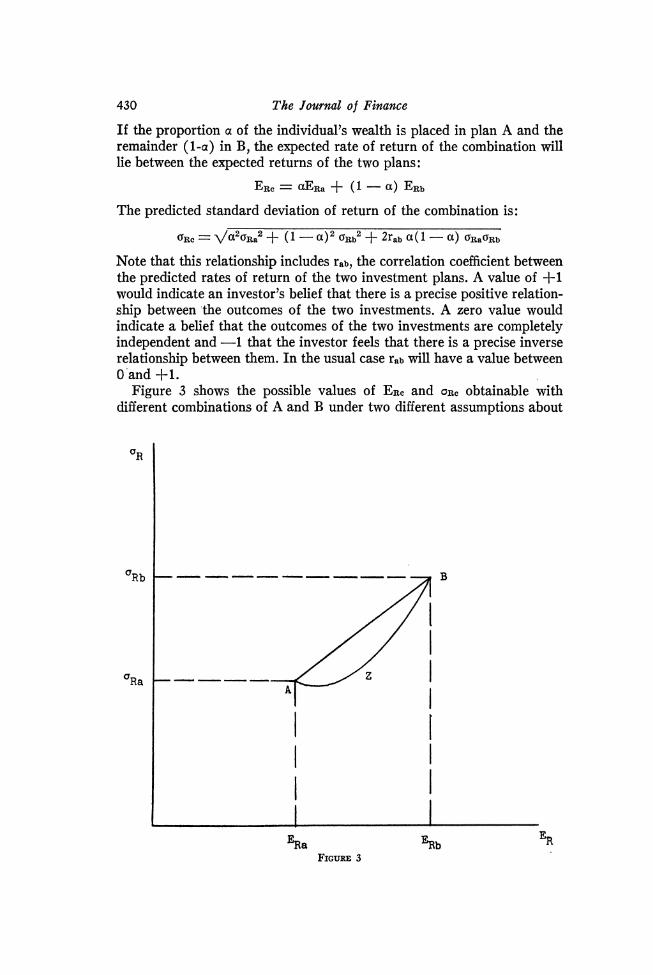
To understand the nature of this curve, consider two investment plans -A and B, each including one or more assets. Their predicted expected values and standard deviations of rate of return are shown in Figure 3.


If the proportion a of the individual's wealth is placed in plan A and the remainder (1-a) in B, the expected rate of return of the combination will lie between the expected returns of the two plans:

The predicted standard deviation of return of the combination is:

Note that this relationship includes lab , the correlation coefficient between the predicted rates of return of the two investment plans. A value of +l would indicate an investor's belief that there is a precise positive relationship between the outcomes of the two investments. A zero value would indicate a belief that the outcomes of the two investments are completely independent and -1 that the investor feels that there is a precise inverse relationship between them. In the usual case rab will have a value between 0 and +l.

Figure 3 shows the possible values of E R ~and OR, obtainable with different combinations of A and B under two different assumptions about

Capital Asset Prices 431

the value of lab . If the two investments are perfectly correlated, the combinations will lie along a straight line between the two points, since in this case both E R ~ and ORC will be linearly related to the proportions invested in the two plans.ll If they are less than perfectly positively correlated, the standard deviation of any combination must be less than that obtained with perfect correlation (since Tab will be less) ; thus the combinations must lie along a curve below the line AB.12 AZB shows such a curve for the case of complete independence (raa = 0) ; with negative correlation the locus is even more U-shaped.13

The manner in which the investment opportunity curve is formed is relatively simple conceptually, although exact solutions are usually quite difficult.14 One first traces curves indicating ER, OR values available with simple combinations of individual assets, then considers combinations of combinations of assets. The lower right-hand boundary must be either linear or increasing a t an increasing rate (d2 O R / ~ E ~ R > 0). AS suggested earlier, the complexity of the relationship between the characteristics of individual assets and the location of the investment opportunity curve makes it difficult to provide a simple rule for assessing the desirability of individual assets, since the effect of an asset on an investor's over-all investment opportunity curve depends not only on its expected rate of return ( E R ~ ) and risk (ON), but also on its correlations with the other available opportunities (ril, riz, . .. . ,ri,). However, such a rule is implied by the equilibrium conditions for the model, as we will show in part IV.

T h e Pure R a t e of Interest

We have not yet dealt with riskless assets. Let P be such an asset; its risk is zero OR^ = 0) and its expected rate of return, E R ~ , is equal (by definition) to the pure interest rate. If an investor places a of his wealth

11. ERc= aERa+ (1-a) ERb= ERb+ (ERa-ERb)a

oRc=da20R,2+ (1-a)2 oRb2+ 2rab a ( l -a) oRa oRb

but rab = 1, therefore the expression under the square root sign can be factored:

oRc= d[aoRa+ (1 - a) oRb12 = a bRa+ (1-a) ORb

= + (oRa-oRb)a 12. This curvature is, in essence, the rationale for diversification.

'Ra 13. When rab = 0, the slope of the curve a t point A is - , a t point B it is

E ~ b-E ~ a GRb . When rab=-1, the curve degenerates to two straight lines to a point

E ~ b-E ~ a on the horizontal axis.

14. Markowitz has shown that this is a problem in parametric quadratic programming. An efficient solution technique is described in his article, "The Optimization of a Quadratic Function Subject to Linear Constraints," Naval Research Logistics Quarterly, Vol. 3 (March and June, 1956), 111-133. A solution method for a special case is given in the author's "A Simplified Model for Portfolio Analysis," op. cit.

432 The Jourtsal of Finance

in P and the remainder in some risky asset A, he would obtain an expected rate of return:

E R ~= a E ~ p+ (1-a) E R ~

The standard deviation of such a combination would be:

but since OR, =0,this reduces to:

This implies that all combinations involving any risky asset or combination of assets plus the riskless asset must have values of ERCand OB,

which lie along a straight line between the points representing the two components. Thus in Figure 4 all combinations of ERand OR lying along

the line PA are attainable if some money is loaned a t the pure rate and some placed in A. Similarly, by lending a t the pure rate and investing in B, combinations along PB can be attained. Of all such possibilities, however, one will dominate: that investment plan lying a t the point of the original investment opportunity curve where a ray from point P is tangent to the curve. I n Figure 4 all investments lying along the original curve


from X to + are dominated by some combination of investment in 4 and lending a t the pure interest rate.

Consider next the possibility of borrowing. If the investor can borrow at the pure rate of interest, this is equivalent to disinvesting in P. The effect of borrowing to purchase more of any given investment than is possible with the given amount of wealth can be found simply by letting a take on negative values in the equations derived for the case of lending. This will obviously give points lying along the extension of line PA if borrowing is used to purchase more of A; points lying along the extension of PB if the funds are used to purchase B, etc.

As in the case of lending, however, one investment plan will dominate all others when borrowing is possible. When the rate a t which funds can be borrowed equals the lending rate, this plan will be the same one which is dominant if lending is to take place. Under these conditions, the investment opportunity curve becomes a line (P+Z in Figure 4). Moreover, if the original investment opportunity curve is not linear at point +,the process of investment choice can be dichotomized as follows: first select the (unique) optimum combination of risky assets (point +), and second borrow or lend to obtain the particular point on PZ at which an indifference curve is tangent to the line.16

Before proceeding with the analysis, it may be useful to consider alternative assumptions under which only a combination of assets lying at the point of tangency between the original investment opportunity curve and a ray from P can be efficient. Even if borrowing is impossible, the investor will choose 4 (and lending) if his risk-aversion leads him to a point below + on the line P+. Since a large number of investors choose to place some of their funds in relatively risk-free investments, this is not an un- likely possibility. Alternatively, if borrowing is possible but only up to some limit, the choice of + would be made by all but those investors willing to undertake considerable risk. These alternative paths lead to the main conclusion, thus making the assumption of borrowing or lending a t the pure interest rate less onerous than it might initially appear to be.

In order to derive conditions for equilibrium in the capital market we invoke two assumptions. First, we assume a common pure rate of interest, with all investors able to borrow or lend funds on equal terms. Second, we assume homogeneity of investor expectations:16 investors are assumed

15. This proof was first presented by Tobin for the case in which the pure rate of interest is zero (cash). Hicks considers the lending situation under comparable conditions but does not allow borrowing. Both authors present their analysis using maximization subject to constraints expressed as equalities. Hicks' analysis assumes independence and thus insures that the solution will include no negative holdings of risky assets; Tobin's covers the general case, thus his solution would generally include negative holdings of some assets. The discussion in this paper is based on Markowitz' formulation, which includes non-negativity constraints on the holdings of all assets.

16. A term suggested by one of the referees.


to agree on the prospects of various investments-the expected values, standard deviations and correlation coefficients described in Part 11. Needless to say, these are highly restrictive and undoubtedly unrealistic assumptions. However, since the proper test of a theory is not the realism of its assumptions but the acceptability of its implications, and since these assumptions imply equilibrium conditions which form a major part of classical financial doctrine, it is far from clear that this formulation should be rejected--especially in view of the dearth of alternative models leading to similar results.

Under these assumptions, given some set of capital asset prices, each investor will view his alternatives in the same manner. For one set of prices the alternatives might appear as shown in Figure 5. In this situa-

tion, an investor with the preferences indicated by indifference curves A1 through A4 would seek to lend some of his funds a t the pure interest rate and to invest the remainder in the combination of assets shown by point 4, since this would give him the preferred over-all position A*. An investor with the preferences indicated by curves BI through B4 would seek to in-vest all his funds in combination +, while an investor with indifference curves CI through C would invest all his funds plus additional (borrowed)


funds in combination 9 in order to reach his preferred position (C*). In any event, all would attempt to purchase only those risky assets which enter combination 9.

The attempts by investors to purchase the assets in combination 9 and their lack of interest in holding assets not in combination 9 would, of course, lead to a revision of prices. The prices of assets in + will rise and, since an asset's expected return relates future income to present price, their expected returns will fall. This will reduce the attractiveness of combinations which include such assets; thus point 9 (among others) will move to the left of its initial position.17 On the other hand, the prices of assets not in 9will fall, causing an increase in their expected returns and a rightward movement of points representing combinations which include them. Such price changes will lead to a revision of investors7 actions; some new combination or combinations will become attractive, leading to different demands and thus to further revisions in prices. As the process con- tinues, the investment opportunity curve will tend to become more linear, with points such as 9 moving to the left and formerly inefficient points (such as F and G) moving to the right.

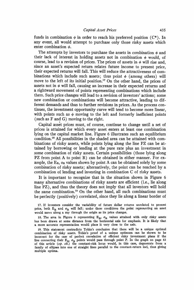
Capital assit prices must, of course, continue to change until a set of prices is attained for which every asset enters a t least one combination lying on the capital market line. Figure 6 illustrates such an equilibrium condition.'' All possibilities in the shaded area can be attained with combinations of risky assets, while points lying along the line PZ can be attained by borrowing or lending at the pure rate plus an investment in some combination of risky assets. Certain possibilities (those lying along PZ from point A to point B) can be obtained in either manner. For example, the ER, OR values shown by point A can be obtained solely by some combination of risky assets; alternatively, the point can be reached by a combination of lending and investing in combination C of risky assets.

I t is important to recognize that in the situation shown in Figure 6 many alternative combinations of risky assets are efficient (i.e., lie along line PZ), and thus the theory does not imply that all investors will hold the same combination.lQ On the other hand, all such combinations must be perfectly (positively) correlated, since they lie along a linear border of

17. If investors consider the variability of future dollar returns unrelated to present price, both E R and aR will fall; under these conditions the point representing an asset would move along a ray through the origin as its price changes.

18. The area in Figure 6 representing ER, crR values attained with only risky assets has been drawn at some distance from the horizontal axis for emphasis. I t is'likely that a more accurate representation would place it very close to the axis.

19. This statement contradicts Tobin's conclusion that there will be a unique optimal combination of risky assets. Tobin's proof of a unique optimum can be shown to be incorrect for the case of perfect correlation of efficient risky investment plans if the line connecting their ER, crR points would pass through point P. In the graph on page 83 of this article (09. cit.) the constant-risk locus would, in this case, degenerate from a family of ellipses into one of straight lines parallel to the constant-return loci, thus giving multiple optima.


the ER, OR region.20 This provides a key to the relationship between the prices of capital assets and different types of risk.

IV. THE PRICES OF CAPITALASSETS We have argued that in equilibrium there will be a simple linear rela-

tionship between the expected return and standard deviation of return for efficient combinations of risky assets. Thus far nothing has been said about such a relationship for individual assets. Typically the ER,QR values associated with single assets will lie above the capital market line, reflect- ing the inefficiency of undiversified holdings. Moreover, such points may be scattered throughout the feasible region, with no consistent relationship between their expected return and total risk (OR). However, there will be a consistent relationship between their expected returns and what might best be called systematic risk,as we will now show.

Figure 7 illustrates the typical relationship between a single capital

20. ER, uR values given by combinations of any two combinations must lie within the region and cannot plot above a straight line joining the points. In this case they cannot plot below such a straight line. But since only in the case of perfect correlation will they plot along a straight line, the two combinations must be perfectly correlated. As shown in Part IV, this does not necessarily imply that the individual securities they contain are perfectly correlated.

Capital Asset Prices 43 7

asset (point i) and an efficient combination of assets (point g) of which it is a part. The curve igg' indicates all ER, OR values which can be obtained with feasible combinations of asset i and combination g. As before, we denote such a combination in terms of a proportion a of asset i and (1 -a) of combination g. A value of a = 1 would indicate pure invest-

ment in asset i while a =0 would imply investment in combination g. Note, however, that a = .5 implies a total investment of more than half the funds in asset i, since half would be invested in i itself and the other half used to purchase combination g, which also includes some of asset i. This means that a combination in which asset i does not appear at all must be represented by some negative value of a. Point g' indicates such a combination.

In Figure 7 the curve igg' has been drawn tangent to the capital market line (PZ) a t point g. This is no accident. All such curves must be tangent to the capital market line in equilibrium, since (1) they must touch it at the point representing the efficient combination and (2) they are con- tinuous a t that point.'l Under these conditions a lack of tangency would

21. Only if rig =-1 will the curve be discontinuous over the range in question.

--


imply that the curve intersects PZ. But then some feasible combination of assets would lie to the right of the capital market line, an obvious impos- sibility since the capital market line represents the efficient boundary of feasible values of ERand aR.

The requirement that curves such as igg' be tangent to the capital market line can be shown to lead to a relatively simple formula which relates the expected rate of return to various elements of risk for all assets which are included in combination g.22Its economic meaning can best be seen if the relationship between the return of asset i and that of combination g is viewed in a manner similar to that used in regression analy- ~ i s . ~ ~Imagine that we were given a number of (ex post) observations of the return of the two investments. The points might plot as shown in Fig. 8. The scatter of the Ri observations around their mean (which will ap- proximate ERI)is, of course, evidence of the total risk of the asset - OR^.

But part of the scatter is due to an underlying relationship with the return on combination g, shown by Big, the slope of the regression line. The response of Ri to changes in R, (and variations in Rg itself) account for

22. The standard deviation of a combination of g and i will be:

= du2oR.,iz+ (1 -aI2uR,2 f 2rig a (1 - a ) aRiuRg a t u = 0:

but a = aRga t a = 0. Thus:

The expected return of a combination will be:

E = aERi + (1 - a ) ERg

Thus, a t all values of a:

and, a t u = 0:

Let the equation of the capital market line be:

aR = s(ER - P) where P is the pure interest rate. Since igg' is tangent to the line when a = 0, and since (ERg, aRg) lies on the line:

URP -=igURi u~€!-

E R ~ E R ~ -PA E R ~ or:

23. This model has been called the diagonal model since its portfolio analysis solution can be facilitated by re-arranging the data so that the variance-covariance matrix becomes diagonal. The method is described in the author's article, cited earlier.

Capital Asset Prices

Return on Asset i (Ri)

Return on Combination g (Rg)

much of the variation in Ri. I t is this component of the asset's total risk which we term the systematic risk. The being uncorrelated with Rg, is the unsystematic component. This formulation of the relationship between Ri and R, can be employed ex ante as a predictive model. Big

becomes the predicted response of Ri to changes in R,. Then, given (the predicted risk of R,), the systematic portion of the predicted risk of each asset can be determined.

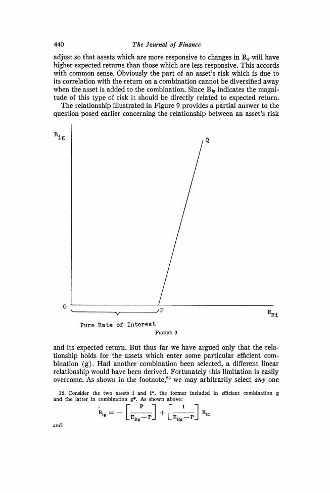
This interpretation allows us to state the relationship derived from the tangency of curves such as igg' with the capital market line in the form shown in Figure 9. All assets entering efficient combination g must have (predicted) Big and ERIvalues lying on the line PQ.26 Prices will

24. ex post, the standard error. 25.

B,,~R,rig = {- = -

~ R I and:

'igb~iBig = -.

~ R P The expression on the right is the expression on the left-hand side of the last equation in footnote 22. Thus:

P 1

ER, -P


adjust so that assets which are more responsive to changes in Rgwill have higher expected returns than those which are less responsive. This accords with common sense. Obviously the part of an asset's risk which is due to its correlation with the return on a combination cannot be diversified away when the asset is added to the combination. Since Bigindicates the magnitude of this type of risk it should be directly related to expected return.

The relationship illustrated in Figure 9 provides a partial answer to the question posed earlier concerning the relationship between an asset's risk

Pure Rate of I n t e r e s t FIGURE9

and its expected return. But thus far we have argued only that the relationship holds for the assets which enter some particular efficient combination (g). Had another combination been selected, a different linear relationship would have been derived. Fortunately this limitation is easily overcome. As shown in the we may arbitrarily select any one

26. Consider the two assets i and i*, the former included in efficient combination g and the latter in combination g*. As shown above:

P 1

~ i .= - -P[-I + [-I ER,

Capital Asset Prices 441

of the efficient combinations, then measure the predicted responsiveness of every asset's rate of return to that of the combination selected; and these coefficients will be related to the expected rates of return of the assets in exactly the manner pictured in Figure 9.

The fact that rates of return from all efficient combinations will be perfectly correlated provides the justification for arbitrarily selecting any one of them. Alternatively we may choose instead any variable perfectly correlated with the rate of return of such combinations. The vertical axis in Figure 9 would then indicate alternative levels of a coefficient measur-ing the sensitivity of the rate of return of a capital asset to changes in the variable chosen.

This possibility suggests both a plausible explanation for the implica-tion that all efficient combinations will be perfectly correlated and a use-ful interpretation of the relationship between an individual asset's ex-pected return and its risk. Although the theory itself implies only that rates of return from efficient combinations will be perfectly correlated, we might expect that this would be due to their common dependence on the over-all level of economic activity. If so, diversification enables the investor to escape all but the risk resulting from swings in economic ac-tivity-this type of risk remains even in efficient combinations. And, since all other types can be avoided by diversification, only the responsiveness of an asset's rate of return to the level of economic activity is relevant in

P 1

' i e g * = - [ E ~ g *-p ] ' [ E R g e - P ] E R i * '

Since Rg and Rgr are perfectly correlated: -- riag

Thus:

Bi*g*%g* Bi*gO,g--'=~i* b ~ i *

and:

Since both g and g* lie on a line which intercepts the E-axis a t P :

-ORe: -- E,g-P

dRgr ERgr-P and:

Thus: P 1 -

ER,* -from which we have the desired relationship between Rie and g:

Bieg must therefore plot on the same line as does Big.


assessing its risk. Prices will adjust until there is a linear relationship between the magnitude of such responsiveness and expected return. As-sets which are unaffected by changes in economic activity will return the pure interest rate; those which move with economic activity will promise appropriately higher expected rates of return.

This discussion provides an answer to the second of the two questions posed in this paper. In Part I11 it was shown that with respect to equilibrium conditions in the capital market as a whole, the theory leads to results consistent with classical doctrine (i.e., the capital market line). We have now shown that with regard to capital assets considered in- dividually, it also yields implications consistent with traditional concepts: it is common practice for investment counselors to accept a lower expected return from defensive securities (those which respond little to changes in the economy) than they require from aggressive securities (which exhibit significant response). As suggested earlier, the familiarity of the implications need not be considered a drawback. The provision of a logical frame- work for producing some of the major elements of traditional financial theory should be a useful contribution in its own right.

capital asset prices: a theory of market equilibrium under ... · capital asset prices 427 asset....

Documents