capital accumulation and unemployment: new insights on the
TRANSCRIPT

IZA DP No. 3066
Capital Accumulation and Unemployment:New Insights on the Nordic Experience
Marika KaranassouHector SalaPablo F. Salvador
DI
SC
US
SI
ON
PA
PE
R S
ER
IE
S
Forschungsinstitutzur Zukunft der ArbeitInstitute for the Studyof Labor
September 2007

Capital Accumulation and Unemployment:
New Insights on the Nordic Experience
Marika Karanassou Queen Mary, University of London
and IZA
Hector Sala Universitat Autònoma de Barcelona
and IZA
Pablo F. Salvador Universitat Autònoma de Barcelona
and Universitat Pompeu Fabra
Discussion Paper No. 3066 September 2007
IZA
P.O. Box 7240 53072 Bonn
Germany
Phone: +49-228-3894-0 Fax: +49-228-3894-180
E-mail: [email protected]
Any opinions expressed here are those of the author(s) and not those of the institute. Research disseminated by IZA may include views on policy, but the institute itself takes no institutional policy positions. The Institute for the Study of Labor (IZA) in Bonn is a local and virtual international research center and a place of communication between science, politics and business. IZA is an independent nonprofit company supported by Deutsche Post World Net. The center is associated with the University of Bonn and offers a stimulating research environment through its research networks, research support, and visitors and doctoral programs. IZA engages in (i) original and internationally competitive research in all fields of labor economics, (ii) development of policy concepts, and (iii) dissemination of research results and concepts to the interested public. IZA Discussion Papers often represent preliminary work and are circulated to encourage discussion. Citation of such a paper should account for its provisional character. A revised version may be available directly from the author.

IZA Discussion Paper No. 3066 September 2007
ABSTRACT
Capital Accumulation and Unemployment: New Insights on the Nordic Experience*
This paper takes a fresh look at the analysis of labour market dynamics and argues that capital accumulation plays a fundamental role in shaping unemployment movements. This role has generally been examined by considering indirect transmission channels of the capital stock effects, i.e. using variables like interest rates or investment ratios in the estimation of single-equation unemployment rate models. Here we advocate a different approach. We directly estimate the effects of capital stock in the labour market by applying the chain reaction theory of unemployment, and we find that capital stock is a major determinant of unemployment in the Nordic countries. In particular, the different unemployment experiences of these economies derive from the temporary (albeit prolonged) negative shocks to capital stock growth in Denmark and Sweden, and the permanent downturn of capital stock growth in Finland. We are thus able to explain why the crisis of the early 1990s had a more acute impact in Finland than in its twin economy, Sweden. JEL Classification: E22, E24, J21 Keywords: unemployment dynamics, chain reaction theory, capital accumulation,
Nordic countries Corresponding author: Hector Sala Departament d’Economia Aplicada Universitat Autònoma de Barcelona 08193 Bellaterra Spain E-mail: [email protected]
* We are grateful to Jaakko Pehkonen for his valuable comments on earlier versions of this paper. Hector Sala is grateful to the Spanish Ministry of Education and Science for financial support through grant SEJ2006-14849/ECON.

1 Introduction
The interest in the capital-unemployment relationship has been revived over the recent
years.1 In this paper we examine the proposition that the slowdown in the growth rate
of capital is responsible for the rise in the unemployment rate. We argue that capital
stock is a determinant of unemployment, both in the short- and the long-run, and show
that capital accumulation can explain the diverse unemployment experiences of the
Nordic countries.
These economies are normally grouped together due to their well developed welfare
state system, low levels of income inequality and successful performance vis-à-vis con-
tinental Europe. Nevertheless, the unemployment trajectories of the three countries in
Figure 1 display significant disparities which are usually overlooked. While Sweden and
Finland came out of the oil crises with hardly any damage, Denmark witnessed a sub-
stantial increase in its unemployment over the late 1970s and early 1980s. In contrast,
although the 1990s crisis first hit Denmark, it did so less intensively than in Sweden
and Finland. We should also note the remarkable similarity in shape, and disparity in
magnitude, of the unemployment paths in these two economies.
The contribution of our work is a country-specific analysis of the Nordic economies
where the evolution of capital accumulation accounts for the above heterogeneities.
A bird’s-eye view of the capital-unemployment relationship in the three countries is
depicted in Figure 2: the correlation between the rates of unemployment and capital
stock growth is -0.67 in Denmark, -0.52 in Sweden, and -0.91 in Finland.
0
2
4
6
8
10
12
74 76 78 80 82 84 86 88 90 92 94 96 98 00 02 04
a. Denmark
0
2
4
6
8
10
70 75 80 85 90 95 00 05
b. Sweden
0
2
4
6
8
10
12
14
16
18
76 78 80 82 84 86 88 90 92 94 96 98 00 02 04
c. Finland
Figure 1. Unemployment rate
There is a tendency in the literature to examine the influence of capital stock on
unemployment by using single unemployment rate equations and proxy variables such
as real interest rates, real balances or investment ratios. There are reasonable doubts1See, among others, Rowthorn (1999), Malley and Moutos (2001), Karanassou and Snower (2004),
and Arestis, Baddeley and Sawyer (2007). A summary documentation of this macro-labour literatureis given in Section 2.
2

as to whether these proxies can capture the effects of capital accumulation net of other
influences.2 Quite often the influence of capital stock is hidden behind non-controversial
accounts of the unemployment upturns due to rises in interest rates or financial crises.
Furthermore, single-equation unemployment rate models cannot take full account of
the transmission channels of the unemployment effects of capital stock (e.g. its effect
on labour demand).
1.5
2.0
2.5
3.0
3.5
4.0
4.5
0 2 4 6 8 10 12
Unemployment rate
Gro
wth
rate
of c
apita
l sto
ck
a. Denmark
0
1
2
3
4
5
0 2 4 6 8 10
Unemployment rate
.b. Sweden
-1
0
1
2
3
4
5
0 5 10 15 20
Unemployment rate
.
c. Finland
Figure 2. Correlation of unemployment and capital accumulation
To explain the unemployment hikes of the 1970s and early 1980s in Denmark, Green-
Pedersen (2001) and Green-Pedersen and Lindbom (2005) point to interest rates as one
of the main driving forces under the deteriorated international wage competitiveness
and the decrease in the terms of trade that pushed unemployment upwards.
Honkapohja and Koskela (1999) attribute the unemployment problem in Finland to
the financial crisis resulting from the pre-1992 overheating of the economy, the collapse
of asset prices and the subsequent high indebtedness of firms and households, which
were worsened with an interest rate rise to defend the exchange rate of the Markka.
We believe that the main manifestation of the Finnish financial crisis is the permanent
drop in its growth rate of capital stock that we identify in Section 5.3
Fregert and Pehkonen (2006) provide a comparative review of some of the most in-
fluential studies analysing the Finnish and Swedish labour markets in the 1990s. Based
2For example, it is certainly true that a fall in interest rates (or a rise in real balances) maycause higher investment and, thereby, larger capital availability and new hirings, but it may also becapturing positive employment effects on account of the enhanced private consumption brought bythis fall (rise). In this case it would be appropriate to include consumption as an explanatory variablein the estimation.
3The fact that Denmark did not suffer a similar banking crisis is attributed by Edey and Hviding(1995) to a more prudential supervision of Danish banks and tighter capital standards.
3

on the combined evidence of the surveyed works and their own estimates they conclude
that the main driving forces of the Finnish unemployment were the rise in interest
rates, productivity shocks and tax changes. Productivity shocks and tax changes were
also significant in Sweden, but with a smaller impact, while interest rates seem to have
played no role.4
This paper measures the unemployment effects of capital accumulation by apply-
ing the Chain Reaction Theory (CRT) of unemployment and estimating a dynamic
multi-equation labour market model with spillover effects (i.e. an interactive dynamics
model).5
Since the unemployment rate is a nontrended variable, single-equation unemploy-
ment models have to use exogenous variables that do not display a trend. This is not
the case with multi-equation labour market models - the only requirement is that each
trended endogenous variable (e.g. employment, real wage, labour force) is balanced
with the set of its explanatory variables. Thus the CRT allows us to evaluate the role
of capital stock on the evolution of unemployment via its influence on labour demand.
The CRT views macroeconomic activity as the result of the interplay between lagged
adjustment processes and changes in the exogenous variables feeding through the labour
market system.6 The lagged adjustment processes are well documented in the literature
and refer, among others, to: (i) employment adjustments arising from labour turnover
costs (hiring, training and firing costs), (ii) wage/price staggering, and (iii) labour force
adjustments.
Within the CRT framework, we focus on the episodes of "high unemployment" in the
Nordic countries and evaluate the extent to which capital accumulation is responsible for
their diverse unemployment upturns over the last decades. Specifically, we examine the
rise in Danish unemployment in the aftermath of the oil price shocks and the substantial
unemployment increases in the early 1990s in all three economies. To establish a link
between these unemployment upturns and the evolution of capital stock, we first identify
the downturns in the growth rate of capital stock using kernel density analysis, and
then conduct dynamic simulations to measure the contributions of capital stock to
unemployment movements. These contributions quantify the unemployment effects of
capital accumulation.
In Denmark, we find that capital stock explains around 30% of the increase in
4Kiander and Pehkonen (1999) point to the rise in interest rates (caused by the high Europeaninterest rates, the speculative attacks against the fixed exchange rate of the Finnish Markka and fasterthan expected disinflation) as the main factor behind the Finnish unemployment increase in the early1990s. For Sweden, Holmlund (2006) argues that the relationship between real interest rates andunemployment is difficult to assess quantitatively and the empirical evidence not conclusive.
5See, for example, Karanassou and Snower (1998), and Karanassou, Sala and Snower (2006a).6The interplay between lagged adjustment processes and growing exogenous variables gives rise to
the phenomenon of frictional growth. For a detailed analysis of the implications of frictional growthsee Karanassou, Sala, and Salvador (2006), and Karanassou and Snower (2007).
4

unemployment in the aftermath of the oil price shocks and near 15% of the increase in
the crisis of the early 1990s. In Sweden, capital accumulation contributes to 50% of the
unemployment upsurge during the 1990s. Finally, the unemployment rate in Finland
would have been 5 percentage points lower in the absence of the 1992 permanent drop
in its capital stock growth rate.
The rest of the paper is structured as follows. Section 2 outlines the macro labour
literature on the effects of capital on unemployment. Section 3 uses an analytic labour
market model to highlight the capital stock-unemployment relationship according to
the chain reaction theory. Section 4 presents the estimated equations for the Nordic
economies. Section 5 associates the episodes of high unemployment in these countries
with the slowdown in the growth rate of their capital stocks. Section 6 concludes.
2 An Overview of the Capital-Unemployment Re-
lationship
The role of capital accumulation in the evolution of the unemployment rate has grad-
ually regained the interest of macro-labour economists and the resulting literature is
extensive and fast growing. We present a selection of papers in chronological order,
and then briefly discuss the labour market doctrine that capital accumulation does not
affect unemployment in the long-run.
Bean and Dréze (1991) focus on the sluggish wage response to the productivity
growth slowdown in Europe in the aftermath of the oil price shocks and show that
wage stickiness reduced employment and, hence, the capital stock profit rate. In turn,
this prompted a decline in investment and capital accumulation that further increased
unemployment.
Phelps (1994, ch. 17) empirically asserts that the unemployment rate is influenced
by trendless transformations of the capital stock such as the ratio of capital to labour
(in efficiency units).
Gordon (1997) argues that the unemployment-productivity tradeoff (UPT) schedule
shifts with movements in capital relative to a fixed level of employment, and finds that
“countries with the largest increases in unemployment had the largest slowdowns in the
growth rate of capital per potential labour hour,” p. 459. However, the UPT schedule
is flat in the long-run, implying no relationship between changes in productivity and
changes in unemployment beyond the medium-term.
Rowthorn (1999) shows that the capital labour ratio affects unemployment in the
long-run when the elasticity of substitution between capital and labour is less than
unity - he finds that this elasticity is, typically, between 0.6 and 0.8.
5

Modigliani (2000) shows that there is a strong negative correlation between the
investment and unemployment rates - this was dubbed the "Modigliani puzzle" by
Blanchard (2000, p. 140).
Arestis and Biefang-Frisancho Mariscal (2000) claim that capital formation is an
important variable in the determination of unemployment and wages. Their model
shows that the NAIRU is a declining function of capital stock and they find significant
effects of capital accumulation on unemployment in the UK and Germany.
Malley and Moutos (2001) show that the unemployment rate is affected in the long-
run when domestic and foreign capital stocks grow at unequal rates.
Karanassou Sala and Snower (2003, 2004) find that the decline in capital formation
is crucial for understanding the EU unemployment experience in the 1970s and 1980s.
Stockhammer (2004) finds that capital accumulation is significantly related to the
unemployment rate in the core European economies and the US. In contrast, he finds
no robust support for the influence of wage-push factors on unemployment.
Karanassou and Snower (2004) show that the long-run unemployment rate depends
on the size of capital stock and that restrictions on the relationships between the long-
run growth rates (as opposed to the levels) of capital stock and other growing exogenous
variables are sufficient for ensuring that the unemployment rate is trendless in the long-
run.
Kapadia (2005) provides an analytic model the link between capital stock and equi-
librium unemployment.
Blanchard (2005) claims that capital accumulation has influenced the evolution of
European unemployment rate over three decades.
Smith and Zoega (2005) find that investment (as a ratio of GDP) has been the
driving force of unemployment in the OECD countries since the 1960s.
Arestis, Baddeley and Sawyer (2007) find a robust negative relationship between
capital accumulation and unemployment in nine EMU countries.
Bande and Karanassou (2007) document the importance of capital stock in explain-
ing the Spanish regional labour market performance.
At the other end of the spectrum lies an influential strand of the literature (see
the prominent work of Layard, Nickel, and Jackman, 1991, hereafter LNJ) arguing
that upward shifts in the time path of capital stock lead to countervailing shifts in the
wage-setting curve so as to restore unemployment to its original long-run equilibrium.
In fact, this hypothesis is the outcome of a specific wage bargaining process charac-
terised by the following two conditions:7 (i) enhanced efficiency - resulting from higher
levels of productivity, quicker capital accumulation or technological change - is trans-
lated into a wage rise by the workers (or their representatives, the unions), and (ii) the
7Wage bargaining processes are modelled via insider-outsider, union or efficiency wage models.
6

reservation wage is a constant proportion of income and changes in line with wages.8
These conditions imply that efficiency gains are absorbed by wage rises and not trans-
lated into employment gains.
The above framework is summarised by the wage setting equation in Blanchard and
Katz (1999, p.69):
(wt − pet) = µbt + (1− µ) yt − βut + εt, (1)
where w is the wage, pe expected prices, b unemployment benefits (proxy of the reserva-
tion wage), y labour productivity, and µ is a parameter such that 0 < µ < 1. Observe
that any increase in y rises real wages by some proportion (1− µ). This could still gen-
erate some employment gains, but these are absorbed by the unemployment benefits.
Combined with the assumption of a unit elasticity of substitution between capital and
labour - typically by assuming a Cobb-Douglas production function - this framework
guarantees that any wage rise due to efficiency gains is translated into higher capital
stock leaving (un)employment unchanged.
The LNJ model forms the basis of the economic policies that claim to reduce un-
employment by suppressing wage-push factors such as unemployment benefits, firing
restrictions, minimum wages, union power or taxes. On one hand, workers’ bargaining
power absorbs productivity gains, and on the other, unemployment benefits lower the
possibility that efficiency gains translate into employment ones. Since the LNJ frame-
work of analysis does not accommodate any influence of capital accumulation on the
unemployment rate, it isolates the labour market from the business cycle and economic
growth branches of macroeconomics.
In contrast, the labour market framework presented below draws from the chain
reaction theory and allows the movements in capital stock to feed through to the un-
employment rate.
3 Capital Stock and the Chain Reaction Theory
The Chain Reaction Theory (CRT) postulates that the evolution of unemployment can
be explained by an interactive dynamics labour market model, i.e. a system of dynamic
equations with spillover effects. Unlike single-unemployment rate models, the CRT
models can also include trended exogenous variables - the only requirement is that each
growing endogenous variable (e.g. employment, real wage, labour force) is balanced
with the set of its explanatory variables.
The analytical model below offers an exposition of the CRT and is in line with the
8It is important to note that unemployment benefits are commonly used as a measure of thereservation wage. Assuming that the latter is a constant proportion of income implies a constantreplacement rate.
7

estimated labour market model presented in the next Section. In particular, we consider
the following labour demand, real wage, and labour supply equations:9
nt = α1nt−1 + β1kt − γ1wt, (2)
wt = α2wt−1 + β2xt − γ2ut, (3)
lt = β3zt + γ3wt, (4)
where nt, wt, and lt denote employment, real wage, and labour force, respectively; kt is
real capital stock, xt represents a wage-push factor, and zt is working-age population; the
β’s, and γ’s are positive constants. The autoregressive parameters α1 and α2 are positive
and less than unity, and can be justified as employment adjustment and wage/price
staggering effects, respectively. All variables are in logs and we ignore the error terms
for ease of exposition. The unemployment rate (not in logs) is10
ut = lt − nt. (5)
We generally refer to lags of the endogenous variables in the labour market model
as the "lagged adjustment processes". Observe that the γ’s generate spillover effects,
since changes in an exogenous variable, say capital stock, can also affect the real wage
and labour supply equations. Thus, in the presence of spillover effects, the short-run
elasticities of the dependent variables with respect to the exogenous ones can no longer
be adequately captured by the β’s. It is worth pointing out that the existence of spillover
effects in a multi-equation model allows us to call it "interactive".
Let us rewrite the demand, wage, and supply equations (2)-(4) as
(1− α1B) (1− α2B)nt = β1 (1− α2B) kt − γ1 (1− α2B)wt, (6)
(1− α2B)wt = β2xt − γ2ut, (7)
(1− α1B) (1− α2B) lt = β3 (1− α1B) (1− α2B) zt + γ3 (1− α1B) (1− α2B)wt,
(8)
where B is the backshift operator, and substitute (7) into (6) and (8) to obtain the
9It can be shown that the labour market model (2)-(4) is compatible with standard microeconomicfoundations. See, for example, Karanassou, Sala, and Snower (2006b).10Since labour force and employment are in logs, the unemployment rate can be approximated by
their difference.
8
following equations for employment and labour force:
(1− α1B) (1− α2B)nt = β1 (1− α2B) kt − γ1β2xt + γ1γ2ut, (9)
(1− α1B) (1− α2B) lt = β3 (1− α1B) (1− α2B) zt + (10)
γ3β2 (1− α1B)xt − γ3γ2 (1− α1B)ut,
respectively.
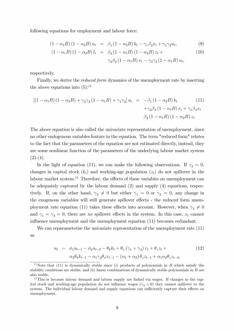
Finally, we derive the reduced form dynamics of the unemployment rate by inserting
the above equations into (5):11
[(1− α1B) (1− α2B) + γ3γ2 (1− α1B) + γ1γ2]ut = −β1 (1− α2B) kt (11)
+γ3β2 (1− α1B)xt + γ1β2xt
β3 (1− α1B) (1− α2B) zt.
The above equation is also called the univariate representation of unemployment, since
no other endogenous variables feature in the equation. The term "reduced form" relates
to the fact that the parameters of the equation are not estimated directly, instead, they
are some nonlinear function of the parameters of the underlying labour market system
(2)-(4).
In the light of equation (11), we can make the following observations. If γ2 = 0,
changes in capital stock (kt) and working-age population (zt) do not spillover in the
labour market system.12 Therefore, the effects of these variables on unemployment can
be adequately captured by the labour demand (2) and supply (4) equations, respec-
tively. If, on the other hand, γ2 6= 0 but either γ1 = 0 or γ3 = 0, any change in
the exogenous variables will still generate spillover effects - the reduced form unem-
ployment rate equation (11) takes these effects into account. However, when γ2 6= 0
and γ1 = γ3 = 0, there are no spillover effects in the system. In this case, xt cannot
influence unemployment and the unemployment equation (11) becomes redundant.
We can reparameterise the univariate representation of the unemployment rate (11)
as
ut = φ1ut−1 − φ2ut−2 − θkkt + θx (γ1 + γ2)xt + θzzt + (12)
α2θkkt−1 − α1γ3θxxt−1 − (α1 + α2) θzzt−1 + α1α2θzzt−2,
11Note that (11) is dynamically stable since (i) products of polynomials in B which satisfy thestability conditions are stable, and (ii) linear combinations of dynamically stable polynomials in B arealso stable.12This is because labour demand and labour supply are linked via wages. If changes in the cap-
ital stock and working-age population do not influence wages (γ2 = 0) they cannot spillover to thesystem. The individual labour demand and supply equations can sufficiently capture their effects onunemployment.
9

where φ1 =α1+α2+α1γ2γ31+γ1γ2+γ2γ3
, φ2 =α1α2
1+γ1γ2+γ2γ3, θk =
β11+γ1γ2+γ2γ3
, θx =β2
1+γ1γ2+γ2γ3, and
θz =β3
1+γ1γ2+γ2γ3.
The reduced form unemployment rate equation (12) displays the following key ele-
ments of the CRT. First, the autoregressive coefficients φ1 and φ2 represent the inter-
actions of the employment adjustment (α1) and wage-price staggering (α2) processes.
Second, the short-run coefficients of the exogenous variables embody the feedback mech-
anisms built in the system, since they are a function of the short-run elasticities/slopes
of the individual equations (2)-(4), i.e. the β’s, and the spillover effects (γ’s). Third,
the interplay of the employment adjustment and wage-price staggering effects, on the
one hand, and the spillover effects, on the other, gives rise to the lags of the exogenous
variables. In time-series jargon, these lags are moving-average terms in (12).
Finally, the capital stock, a trended variable, features as a driving force of the
unemployment rate, a stationary variable. This is a controversial and hotly debated
result that we can justify as follows. Capital stock initially enters the system as a
determinant of employment, a trended variable. Labour demand (2) is a balanced
equation since it is dynamically stable (|α1| < 1) . Similarly, the trended labour forceis driven by working-age population (also a trended variable), and the static labour
supply (4) is itself a balanced equation. According to (9)-(10), the labour demand and
supply equations remain balanced once the wage (3) has been substituted into them.13
Therefore, the "reduced" unemployment rate equation is itself balanced, since (by
(5)) it is given by the difference of the dynamically stable labour supply and demand
equations. As mentioned in Section 2, Karanassou and Snower (2004) show that equili-
brating mechanisms in the labour market and other markets jointly act to ensure that
the unemployment rate is trendless in the long-run. These mechanisms can be expressed
in the form of restrictions on the relationships between the long-run growth rates of
capital stock and other growing exogenous variables.14
13Note that (9) and (10) are dynamically stable since the products of polynomials in B which satisfythe stability conditions are also stable.14Given the labour market model (2)-(5), it can be shown that the unemployment rate stabilises in
the long-run if
β1 (1− α2) gk = β3 (1− α1) (1− α2) gz +
[β2γ1 + β2γ3 (1− α1)] gx,
where gk, gz, and gx denote the long-run growth rates of capital stock, working-age population, andthe wage-push factor, respectively. If xt does not grow in the long-run, the restriction simplifies toµ
β11− α1
¶gk = β3gz.
10

4 Econometric Analysis
The empirical models presented below are in line with the consensus view of the labour
market, according to which (i) labour demand is negative along the real wage and shifts
with changes in capital stock, (ii) rises in capital deepening (a proxy for productivity)
increase real wages, and (iii) labour supply is positive along the real wage. Furthermore,
the common structure shared by the estimated equations facilitates comparisons among
the three countries.
4.1 Data and Methodology
The dataset is obtained from the OECDEconomic Outlook and the sample period of our
analysis is 1973-2005 for Denmark, 1976-2005 for Finland, and 1966-2005 for Sweden.
Table 1 gives the definitions of the variables included in the selected equations.15
Table 1: Definitions of variables.n employment (log) r real long-term interest ratel labour supply (log) fd exports-imports (% of GDP)w real compensation per employee (log) τd direct tax rates (% of GDP)u unemployment rate (l − n) τ i indirect tax rates (% of GDP)k real capital stock (log) g public expenditures (% of GDP)kn capital stock per employee (k − n) τw fiscal wedge16
z participation rate³
labour forceworking-age population
´o real oil prices (log)
Source: OECD, Economic Outlook.
The estimation strategy involves the Autoregressive Distributed Lagged (ARDL)
approach developed by Pesaran (1997), Pesaran and Shin (1999) and Pesaran, Shin
and Smith (2001). The justification of this choice can be summarised as follows. It
has been shown that the ARDL yields consistent estimates both in the short- and long-
run, and can be reliably used in small samples for hypothesis testing irrespective of
whether the regressors are I(1) or I(0). Therefore, the ARDL offers an alternative to the
popular cointegration/error-correction methodology that avoids the pretesting problem
implicit in the standard cointegration techniques - the Johansen maximum likelihood,
and the Phillips-Hansen semi-parametric, fully-modified OLS procedures. Furthermore,
Pesaran and Shin (1999) argue that the Phillips-Hansen and ARDL approaches are
directly comparable, and the estimator of the former is outperformed by the ARDL
estimator, especially when the sample size is relatively small (as in our case).
15Note that we have experimented with a wider set of exogenous variables - social security benefitsand contributions, measures of competitiveness, financial wealth, real money balances, and consump-tion - but these were found to have no explanatory power on the endogenous variables.16The fiscal wedge is the sum of direct, indirect and payroll taxes as a ratio of total compensation
of employees.
11

Our dynamic labour market model comprises labour demand, wage setting, and
labour supply equations:17
A0yt =2X
i=1
Aiyt−i +2X
i=0
Dixt−i + εt, (13)
where yt is a (3× 1) vector of endogenous variables (employment, real wage, and labourforce) xt is a (9× 1) vector of exogenous variables, the Ai’s and Di’s are (3× 3) and(9× 9), respectively, coefficient matrices, and εt is a (3× 1) vector of strict white noiseerror terms.
Each equation of the labour market system (13) is estimated following the ARDL
approach and the selected specifications pass a battery of diagnostic tests for serial
correlation, linearity, normality, heteroskedasticity and autoregressive conditional het-
eroskedasticity, and structural stability. Finally, to account for potential endogeneity
and cross equation correlation we estimate the labour market model for each country
with 3SLS. These estimated equations, together with the definition (5), are then used
to obtain the "reduced form" unemployment rate equation underlying the rest of our
empirical analysis.
In what follows we discuss our estimation results and provide an overall evaluation
of the selected labour market models.18
4.2 Labour demand
Table 2 reports the 3SLS estimates of the employment equation for the three countries.
It is worth observing the different employment persistence across countries. Labour
demand in Denmark displays the lowest persistence coefficient, 0.18, indicating a quick
speed of adjustment to economic disturbances. This may reflect the high degree of
flexibility which characterises the Danish labour market (the employment protection
legislation is among the less strict in the OECD countries). In turn, the persistence
coefficients in Sweden and Finland are substantially higher and amount to 0.66 and
0.64, respectively. Note that in Sweden the multiplicative dummies, nd1t−1 and nd2t−1,
take into account the significant decrease in employment persistence over 1991-2005.19
17The dynamic system (13) is stable if, for given values of the exogenous variables, all the roots ofthe determinantal equation ¯̄
A0 −A1B −A2B2¯̄= 0
lie outside the unit circle. Note that the estimated equations given below satisfy this condition.18Although Tables 2-4 below only give the 3SLS results, the OLS estimates together with the results
on the misspecification tests are available upon request.19We believe the decrease in persistence over that period is related to the boost in the active labour
market programmes (ALMPs) - with increases in the volume of training programmes and expansion ofsubsidised employment and youth practice programmes - and the extension of the maximum permittedduration for probationary contracts from 6 to 12 months. Note that ndit−1 = di × nt−1, for i = 1, 2,
12

Table 2: Labour demand equations - Dependent variable: nt.
Denmark (1973-2005) Sweden (1966-2005) Finland (1976-2005)const. 11.6 [0.000] const. 2.88 [0.046] const. 2.95 [0.004]nt−1 0.18 [0.144] nt−1 0.66 [0.000] nt−1 0.64 [0.000]∆nt−1 0.61 [0.000] nd1t−1 -0.001 [0.140] ∆nt−1 0.19 [0.046]wt -0.58 [0.009] nd2t−1 -0.003 [0.005] wt 0.71 [0.000]wt−1 -0.30 [0.052] wt -0.78 [0.000] wt−1 -0.95 [0.000]kt 0.48 [0.000] wt−1 0.67 [0.000] kt 0.28 [0.001]∆kt 1.78 [0.000] kt 0.22 [0.002] ∆kt 1.87 [0.001]∆kt−1 1.14 [0.082] ∆kt 2.56 [0.000] rt -0.34 [0.009]gt 1.02 [0.001] τ it -1.08 [0.004] fdt 0.34 [0.007]∆gt -0.89 [0.011]∆gt−1 0.95 [0.003]
R2 0.981 0.935 0.971∆ denotes the difference operator; p-values in square brackets.
The effect of capital stock is significant in all three economies, with a long-run
elasticity of 0.6 in Denmark (i.e. a 1% rise in k boosts employment by 0.6%), 0.7
in Sweden, and 0.8 in Finland. Note that all these values are in the range given by
Rowthorn (1999).
Furthermore, employment in Denmark is very sensitive to wage variations; the long-
run elasticity of almost negative unity comes as no surprise in such a flexible labour
market. The long-run wage elasticities in Sweden and Finland are -0.3 and -0.7, respec-
tively. The latter is in line with Kiander and Pehkonen (1999) who show that wages
affect the Finnish labour demand with an elasticity between -0.3 and -0.8, depending
on the sample period.
Further to the above common determinants, we have also identified idiosyncratic
influences. Government expenditures in Denmark, indirect taxes in Sweden, and real
interest rates and foreign demand in Finland.
The strong influence of government expenditures on the Danish economy relates to
the fact that its public sector is responsible for the production of the vast majority of
services and accounts for almost a third of total employment.20 The role of interest
rates in the Finnish unemployment rate has been extensively studied by Kiander and
Pehkonen (1999), Honkapohja and Koskela (1999) and Fregert and Pehkonen (2006). In
turn, the presence of foreign demand captures the important export-led recovery of the
Finnish economy during the last decades, a phenomenon that Kiander and Pehkonen
(1999) found significant in explaining the unemployment trajectory.
where the dummy d1 takes the value 1 over the period 1991-1994, zero otherwise, and the dummy d2takes the value 1 over the period 1995-2005, zero otherwise.20See Karanassou, Sala and Salvador (2006) for a detailed analysis of the Danish labour market.
13

4.3 Wage setting
Table 3 below presents the 3SLS estimates of the real wage equation for the three
countries.
Similarly to the labour demand, wage setting exhibits different degrees of persistence
across countries. As expected, the quickest adjustment takes place in Denmark, where
the inertia coefficient is 0.32, with Sweden, 0.62, and Finland, 0.80, displaying more
sluggishness.
Table 3: Wage setting equations - Dependent variable: wt.
Denmark (1973-2005) Sweden (1966-2005) Finland (1976-2005)const. 5.34 [0.000] const. 3.24 [0.000] const. 1.52 [0.037]wt−1 0.32 [0.003] wt−1 0.62 [0.000] wt−1 0.80 [0.000]∆wt−1 0.44 [0.000] ∆wt−1 0.21 [0.046]ut -0.60 [0.000] ut -0.67 [0.004] ut -0.59 [0.000]knt 0.31 [0.000] knt 0.31 [0.000] knt 0.22 [0.039]rt 0.38 [0.000] τdt 0.63 [0.004] τwt 0.27 [0.008]
τdt−1 -0.46 [0.056] ot 0.02 [0.003]τ it -0.78 [0.003]
R2 0.995 0.995 0.995∆ denotes the difference operator; p-values in square brackets.
Furthermore, wages in all three countries are influenced by unemployment and capi-
tal deepening with the expected negative and positive signs, respectively. It is important
to note that capital deepening (defined as the log of capital stock per employee) is a
standard proxy of (the log of) labour productivity and several studies document its
significance in the Nordic economies - Hansen and Warne (2001) in Denmark, Hjelm
(2006) in Sweden, and Kiander and Pehkonen (1999) in Finland. In particular, the
latter find that capital deepening is the most important factor in wage setting with
a long-run elasticity close to unity. In our estimations, the long-run "productivity"
elasticity of wage is close to unity in Sweden and Finland (0.82 and 1.10, respectively),
while in Denmark it is only 0.46.
The absence of social security benefits and contributions from our estimations may
appear striking, at first sight, given the important role usually assigned to these institu-
tional variables. Note, however, that wage setting in Finland is influenced by the fiscal
wedge, while wages in Sweden are affected by direct and indirect taxes. These results
are consistent with other findings in the literature. Pehkonen (1999), and Kiander and
Pehkonen (1999) outline the harmful employment effects of the steady growth in the
fiscal wedge via the increasing wage pressure brought by the higher income and payroll
14

taxes used to finance the Finnish pension and unemployment insurance systems. Re-
garding Sweden, the significance of taxes is also acknowledged by Forslund (1995), and
Fregert and Pehkonen (2006), among others. We can thus argue that taxes and fiscal
wedge capture the effect of wage push factors, such as benefits and contributions, in
wage setting.
In Denmark, real interest rates contribute positively to real wages due to their
downward pressure on prices.21 Finally, the sensitivity of wages to oil prices, in Finland,
signifies the exposure of this labour market to external shocks (see also Honkapohja and
Koskela, 1999).
4.4 Labour supply
Table 4 below gives the 3SLS estimates of the labour force equation for the three
countries.
In contrast with labour demand and wage setting, labour supply in Denmark features
the highest persistence among the three economies. Note also that, while in Sweden
and Finland stickiness in labour supply decisions does not differ substantially from that
of labour demand and wage setting, in Denmark labour market flexibility is attained
via quick labour demand and wage adjustments.
Table 4: Labour supply equations - Dependent variable: lt.
Denmark (1973-2005) Sweden (1966-2005) Finland (1976-2005)const. 1.24 [0.000] const. 4.55 [0.000] const. 3.76 [0.000]
lt−1 0.90 [0.000] lt−1 0.64 [0.000] lt−1 0.70 [0.000]∆lt−1 0.76 [0.000] ∆lt−1 1.33 [0.000]
∆lt−2 -0.33 [0.000] ∆lt−2 0.03 [0.053]∆ut -0.04 [0.031] ut -0.32 [0.000] ∆ut -0.08 [0.000]
∆ut−1 -0.04 [0.035] ∆ut−1 -0.01 [0.444]wt 0.02 [0.004] wt 0.08 [0.000] wt 0.05 [0.000]
∆wt -0.03 [0.035] ∆wt -0.03 [0.027]zt 0.18 [0.000] zt 0.32 [0.000] zt 0.42 [0.000]
∆zt 1.09 [0.000] ∆zt 0.85 [0.000]∆zt−1 -1.04 [0.000] ∆zt−1 -1.86 [0.000]
R2 0.999 0.995 0.999∆ denotes the difference operator; p-values in square brackets.
The role of wages and unemployment in labour supply decisions of the three countries
is as expected. Wages exert an overall positive influence, while unemployment has a
21Note that the effect of interest rates on unemployment is the expected negative one, since wagesenter negatively in labour demand.
15

negative effect (in Denmark and Finland via a discouraged workers effect, in Sweden
through the level of unemployment).
Finally, it is through the participation rate instead of the working age population
that we can capture demographic influences on the labour supply movements. We
explain this finding by recognising that the participation rate reflects both cultural -
the society’s attitude towards the labour market - and institutional features that have
led the Nordic countries to have the highest (female and youth) participation rates in
the OECD.
In particular, Denmark is the sole country where participation rates have stayed
above 80% - the highest in the OECD countries - since the mid 1980s that the economy
had recovered from the oil price crises. This is due to the system of Active Labour Mar-
ket Policies characterising the Danish labour market that dates back to 1979. Its main
objective is to promote labour market participation, thus avoiding labour shortages and
ensuring the sustainability of public finances (see Andersen, 2006, and Plougmann and
Madsen, 2005).
4.5 Evaluation of the Models
We further evaluate our empirical models with two auxiliary diagnostics. First, we
test whether the long-run relationships implied by our estimations comprise cointegrat-
ing vectors within the Johansen framework. Once the maximal eigenvalue and trace
statistics confirm that the variables involved in each equation are cointegrated, the Jo-
hansen’s cointegrating vectors are restricted to take the corresponding long-run values
of our estimated equations. Table 5 displays the LR tests following a χ2 (·) distribu-tion.22 Observe that the restrictions cannot be rejected at conventional sizes of the test,
indicating that the estimation methodology we followed conforms with the Johansen
procedure.
Table 5: Testing the long-run relationships in the Johansen framework
Labour demand Wage setting Labour force
Denmark χ2 (2) =8.79 [0.012] χ2 (2) =1.87 [0.393] χ2 (1) =0.24 [0.622]Finland χ2 (2) =1.08 [0.582] χ2 (2) =2.78 [0.249] χ2 (1) =2.90 [0.089]Sweden χ2 (2) =1.89 [0.388] χ2 (2) =1.05 [0.591] χ2 (1) =2.52 [0.113]
p-values in square brackets.
22It should be noted that we only consider the I(1) variables in our models: nt, wt, lt, and kt (recallthat knt = kt−nt). Therefore, we test two restrictions in the labour demand and wage setting equationsand one in the labour suply equation. To conserve space, we do not report the results of the underlyingunit root tests and the details of the cointegration analysis - these are available upon request.
16

Second, we check the model’s ability to replicate the actual facts. As Figure 3 shows,
the estimated labour market models track actual unemployment very closely in all three
countries - the only exception is the early part of the sample for Sweden. However, we
do not find this discrepancy unsettling, since it is probably due to shocks affecting the
foreign sector of the Swedish economy (e.g. devaluations) that dissipated by the late
1970s. In addition, the 1990s slump which is the central focus of our analysis is tracked
very precisely.
0
2
4
6
8
10
12
75 80 85 90 95 00 05
ActualFitted
a. Denmark
0
2
4
6
8
10
70 75 80 85 90 95 00 05
ActualFitted
b. Sweden
0
2
4
6
8
10
12
14
16
18
80 85 90 95 00 05
ActualFitted
c. Finland
Figure 3. Unemployment rate: actual and fitted values
5 Contributions of Capital Accumulation to Unem-
ployment
The Nordic countries are generally treated as a relatively homogenous area which is
compared with other groups such as the Continental European or the Anglo-Saxon
economies. However, the plots in Figure 3 evidence the significant disparities in the
unemployment trajectories of the three countries.
17
In the last decades Denmark has experienced two periods of rising unemployment,
the first one in the aftermath of the oil price shocks with a rise of 8 percentage points
(from 0.8% in 1973 to 8.8% in 1983), and the second one in the late 1980s and early
1990s with the unemployment rate doubling from 5.1% in 1987 to 10.0% in 1993.
In contrast, the Finnish and Swedish experiences are characterised by a long period
of low unemployment lasting until the end of the 1980s, which was abruptly terminated
in the early 1990s. For this, and other reasons, these two countries are sometimes
referred to as the "twin economies," even though their unemployment trajectories dis-
play clear differences in terms of magnitudes. For example, the rate of unemployment
in Sweden was on average 2.5-3 percentage points lower than that in Finland during
the "full-employment" period. In the recession of the early 1990s, the Swedish unem-
ployment rate never exceeded 8.6%, while the Finnish unemployment rate was pushed
to a high of 18.2%. Finally, in the subsequent recovery, the difference between the two
unemployment rates remained above 5 percentage points until 2003.
In what follows we argue that the evolution of capital stock accumulation can ac-
count for the disparities in the unemployment trajectories of the Nordic economies. In
particular, we show that, feeding through the labour market system, the investment
downturns give rise to the unemployment rate upturns and drive their intensity and
longevity.
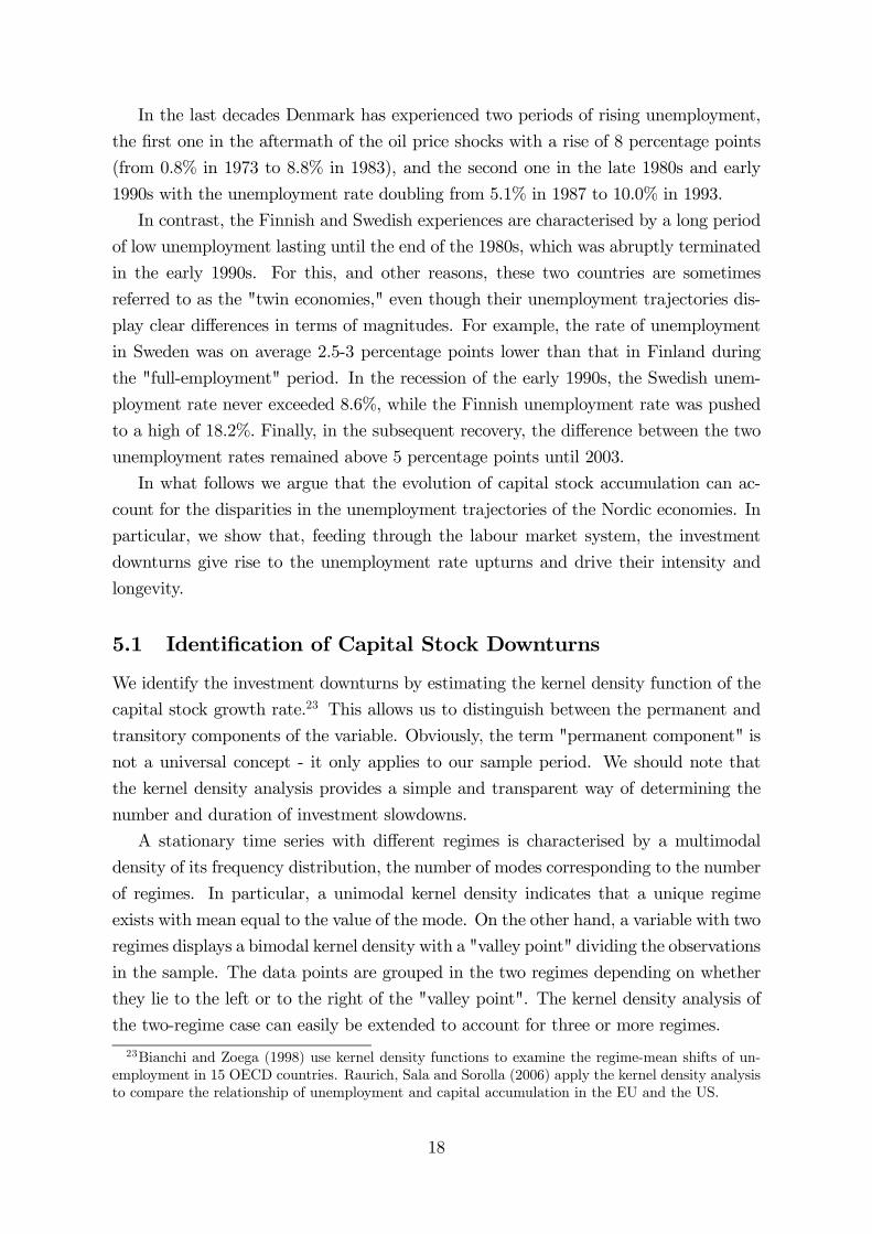
5.1 Identification of Capital Stock Downturns
We identify the investment downturns by estimating the kernel density function of the
capital stock growth rate.23 This allows us to distinguish between the permanent and
transitory components of the variable. Obviously, the term "permanent component" is
not a universal concept - it only applies to our sample period. We should note that
the kernel density analysis provides a simple and transparent way of determining the
number and duration of investment slowdowns.
A stationary time series with different regimes is characterised by a multimodal
density of its frequency distribution, the number of modes corresponding to the number
of regimes. In particular, a unimodal kernel density indicates that a unique regime
exists with mean equal to the value of the mode. On the other hand, a variable with two
regimes displays a bimodal kernel density with a "valley point" dividing the observations
in the sample. The data points are grouped in the two regimes depending on whether
they lie to the left or to the right of the "valley point". The kernel density analysis of
the two-regime case can easily be extended to account for three or more regimes.
23Bianchi and Zoega (1998) use kernel density functions to examine the regime-mean shifts of un-employment in 15 OECD countries. Raurich, Sala and Sorolla (2006) apply the kernel density analysisto compare the relationship of unemployment and capital accumulation in the EU and the US.
18

Naturally, when the variable is characterised by one regime, this is taken to be
permanent. For multimodal kernel densities we distinguish between permanent and
temporary regimes and identify them as follows. The variable starts in one regime (say,
A) in the beginning of the sample, and then moves to another regime (say, B) at some
later point in time. If the variable reverses to regime A before the end of the sample,
then regime B is temporary and regime A is permanent. On the other hand, if the
variable stays in regime B by the end of the sample then both regimes are permanent
ones.
0.0
0.2
0.4
0.6
0.8
2.0 2.5 3.0 3.5 4.0 4.5
a. Kernel density analysis
Permanent regime,mean = 3.6%
1.5
2.0
2.5
3.0
3.5
4.0
4.5
75 80 85 90 95 00 05
b. Capital accumulation
Actual trajectory (solid line)Permanent component (dotted line)Temporary downturns (shadded areas)
0.0
0.1
0.2
0.3
0.4
1 2 3 4 5
c. Kernel density analysis
Permanent regime,mean = 3.3%
0
1
2
3
4
5
70 75 80 85 90 95 00 05
d. Capital accumulation
Actual trajectory (solid line)Permanent component (dotted line)Temporary downturn (shadded area)
0.00
0.05
0.10
0.15
0.20
0.25
0.30
-1 0 1 2 3 4 5
e. Kernel density analysis
Permanent regime,mean = 0.8%
Permanent regime,mean = 2.9%
Regime changeat 1.9%
-1
0
1
2
3
4
5
80 85 90 95 00 05
f. Capital accumulation
Low regimemean at 0.8%
High regime mean at 2.9%
Actual trajectory (solid line)Permanent components (dotted lines)
Figure 4. Capital accumulation in the Nordic countries
Denmark
Sweden
Finland
19

The plots of the kernel density functions in the first column of Figure 4 reveal the
number of regimes for the capital stock growth rates of the Nordic economies. The
plots in the second column of Figure 4 display the actual series (solid lines) and the
mean values of their permanent regimes (dotted lines).
According to Figure 4a, the growth rate of capital stock in Denmark displays a single
regime with mean 3.6%. Figure 4b shows that Denmark experienced two downturns in
investment over the 1978-1985 and 1989-1997 periods with the growth rate of capital
stock reaching a low of 2.0% in 1981 and 2.6% in 1993.
Figure 4c shows that the growth rate of capital stock in Sweden is also characterised
by one regime with mean 3.3%. A temporary but prolonged downturn took place from
1991 to 1997 (see Figure 4d). In 1990 capital accumulation declined sharply from 3.9%
to 1.0% in 1993; it slowly recovered afterwards to reach its structural level by 1998.
In contrast to Denmark and Sweden, capital accumulation in Finland displays two
regimes (see Figure 4e-f). While the growth rate of capital stock fluctuates around 2.9%
until 1991, it hovers around 0.8% after 1992. The slowdown in investment that persists
after the 1992 structural break accompanies, strikingly well, the high unemployment
era in Finland with rates between 9% and 18%. Thus, the kernel density analysis helps
us to understand the extremely high negative correlation between the unemployment
and capital stock growth rates documented in Figure 2c.
To evaluate the unemployment contributions of the above identified downturns in
capital accumulation we simulate the estimated labour market model with a capital
stock series that we construct by using the permanent component of capital accumula-
tion (dotted line in Figures 4b, 4d, 4f), instead of the actual series (solid line in Figures
4b, 4d, 4f).
5.2 Denmark: the ‘Anglo-Saxon’ Nordic Economy
In Denmark, we measure the unemployment effects of capital accumulation as follows.
First, we simulate the Danish labour market model over the period of the first slowdown
in the growth rate of capital stock, 1978-1985, using a capital stock series constructed
by the 1978-1985 segment of the dotted line in Figure 4b. As shown Figure 5a, the
persistent shock of the second half of the 1970s and first half of the 1980s accounts
for a substantial part of the increase in Danish unemployment during this period. The
unemployment rate would have been, on average, 2 percentage points lower: 5.0%
instead of 7.0%. Therefore, almost 30% of unemployment in the 1978-1985 period can
be explained by the decline in capital formation.
Second, we run an analogous simulation for the labour market model over the 1989-
1997 capital accumulation slowdown. Figure 5b shows that, had the growth rate of
20

capital stock remained at its structural path (dotted line in Figure 4b), unemployment
would have been relatively stable (around 7%) in the early 1990s, reaching a maximum
in 1993 of 7.5% instead of its actual 10% peak. In addition, the average rate of un-
employment during the 1989-1997 period would have been 6.6%, one percentage point
lower than its actual value.
0
2
4
6
8
10
74 76 78 80 82 84 86
a. Early 1980s downturn
Actualtrajectory
Simulated (in the absence of the1978-1985 prolonged shock)
4
5
6
7
8
9
10
11
88 90 92 94 96 98 00 02 04
b. Early 1990s downturn
Actualtrajectory
Simulated (in theabsence of the1989-1997prolonged shock)
Figure 5. Unemployment effects of capital accumulation in Denmark
8787
According to Honkapohja and Koskela (1999), and Koskela and Uusitalo (2006),
among others, the second upturn in unemployment was prompted by the international
recession and the 1989 German unification which raised interest rates all around Europe.
Hence, real interest rates were a major contributor to the onset of this crisis. This
meshes well with our own analysis since it is plausible to argue that the rise in interest
rates is manifested in the investment slowdown after 1989.
5.3 The ‘Twin Economies’ and the 1990s Slump
The message conveyed by the plots in Figure 1 is that the unemployment rate time
paths of Sweden and Finland are rescaled versions of one another. Hence the reference
to the two countries as the ‘twin economies’. Below we argue that the much higher
unemployment rates experienced by Finland after 1992 are due to the permanent decline
in the growth rate of its capital stock occurring in 1992 (see Figures 4e-f). By contrast,
in Sweden, the substantial slowdown in capital accumulation in 1991 has been reversed
by 1997 (see Figures 4c-d).
In other words, the capital accumulation downturn in Sweden is transitory and we
measure its effects on unemployment similarly to Denmark. We simulate the Swedish
labour market model over the 1991-1997 period of the slowdown in investment, using a
21

capital stock series constructed by the 1991-1997 segment of the dotted line in Figure
4d. Therefore, the dotted line in Figure 6a gives the time path that the unemployment
rate would have followed had capital stock continued to grow at 3.2% from 1991 to
1997. Note that while actual unemployment sharply rises to a maximum of 8.6% in
1993 and then stabilises at values above 8%, the simulated series reaches its peak of
6.3% in 1998. Furthermore, the average unemployment rate would have been of 3.6%
instead of 7.2%, and so the capital accumulation downturn accounts for 50% of the
unemployment problem over the 1991-1997 period.
0
2
4
6
8
10
70 75 80 85 90 95 00 05
a. Impact of the prolonged downturn in Sweden
Actualtrajectory
Simulated (in theabsence of the1990-1997prolonged shock)
0
2
4
6
8
10
12
14
16
18
76 78 80 82 84 86 88 90 92 94 96 98 00 02 04
Actual trajectory
Simulated (incidenceof the permanent regimechange removed fromactual unemployment)
b. Impact of the permanent downturn in Finland
Figure 6. Unemployment effects of capital accumulation in Sweden and Finland
The kernel density analysis in Figures 4e-f shows that the 1992 structural break
pushed the growth rate of capital stock in Finland from a high regime with mean 2.9%
to a low regime with mean 0.8%. We evaluate the impact of the permanent decrease in
capital accumulation after 1992 as follows.
We simulate the steady state of the Finnish labour market model under two scenarios
1992 onwards: (i) a capital stock growing at 2.9%, and (ii) a capital stock growing at
0.8%. The reason for simulating the steady-state of the model is that we want to
measure the effect of the permanent shift in the growth rate of the capital stock net
of the lagged adjustments present in the labour market. The difference between the
two simulated time paths of the unemployment rate is around 5 percentage points and
is our measure of the unemployment contribution of the permanent decline in capital
accumulation after 1992. We subtract this contribution from the actual unemployment
rate and plot the resulting series in Figure 6b (dotted line).
Figure 6b shows that had capital growth remained at its high regime mean, unem-
ployment would have peaked at 13.4% in 1994 instead of the actual 18.2%. In turn, the
actual subsequent fall to around 9% in 2005 would have ended up near 4.0%. This result
22

has two important implications. First, the magnitudes of the Finnish unemployment
trajectory would have been much closer to the Swedish ones. We have thus identified
a crucial factor explaining the disparity in the intensity of the early 1990s crisis in the
so-called twin economies. Second, in the absence of the permanent slowdown in in-
vestment after 1992, Finland would have recovered the full-employment levels that had
historically characterised its labour market.
Our analysis is consistent with the view of Honkapohja and Koskela (1999) that
external shocks (the collapse of trade with the Soviet Union, the western recession and
the rise in German interest rates) are not the main driving forces of the unemployment
rate in Finland.
6 Conclusions
In this paper we showed that capital accumulation plays a significant role in explaining
the diverse unemployment experiences of the Nordic countries.
Following the chain reaction theory (CRT) of unemployment, we estimated a dy-
namic labour market model with spillover effects that allows the interplay of the move-
ments in capital stock and lagged adjustment processes to feed through to the unemploy-
ment rate. Using kernel density analysis, we identified the temporary and permanent
slowdowns in capital accumulation and, focusing on the relatively high unemployment
periods, we performed dynamic simulations and showed that the downturns in capital
accumulation drive the intensity and longevity of the upturns in unemployment.
In particular, the unemployment swings in Denmark resemble those of the US, with
peaks in the early 1980s and 1990s, hence the reference to it as the ‘Anglo-Saxon’
Nordic economy. We found that the persistent capital stock shocks of 1978-1985 and
1989-1997 account for approximately 30% and 15% of the rise in unemployment during
these periods, respectively.
Finland and Sweden are labelled the ‘twin economies’ due to the similarity in their
unemployment trajectories: they came out of the oil price shocks with no serious damage
and faced unprecedented unemployment increases in the early 1990s. Nevertheless, the
gap in the unemployment rates of the two countries in the aftermath of the 1990s crisis
was substantial, reaching almost 10 percentage points. In Sweden, we found that the
1991-1997 slowdown in capital accumulation contributes to 50% of the unemployment
increase during this period. Finland, unlike Denmark and Sweden, is characterised
by a permanent drop in capital accumulation since 1992. Had capital accumulation
remained at its high-regime mean, unemployment would have been 5 percentage points
lower and the unemployment gap in the twin economies would have been substantially
reduced 1992 onwards.
23
Our results shift the emphasis in the determinants of unemployment from wage-
push factors to capital accumulation. Instead of following the conventional policy recipe
attempting to reduce unemployment by suppressing wage-push factors (such as unem-
ployment benefits, firing restrictions, minimum wages, union power, taxes), our analysis
offers a way of explaining the unemployment problem by recognising the interaction of
growth and dynamics in the labour market. The significant unemployment contribu-
tions of capital accumulation imply that policies related to R&D activities, policies
promoting innovations and productivity growth, or policies directly fostering invest-
ment and capital accumulation, can enhance the performance of the labour market.
References[1] Andersen, T. (2006): “From Excess to Shortage — Recent Developments in the Danish
Labour Market,” in M. Werding (ed.) Structural Unemployment in Western Europe:Reasons and Remedies, The MIT Press, Cambridge MA, pp. 75-102.
[2] Arestis, P. and I. Biefang-Frisancho Mariscal (2000): “Capital Stock, Unemploymentand Wages in the UK and Germany,” Scottish Journal of Political Economy, 47 (5), pp.487—503.
[3] Arestis, P., M. Baddeley and M. Sawyer (2007): “The relationship between capital stock,unemployment and wages in nine EMU countries,” Bulletin of Economic Research, forth-coming.
[4] Bande, R. and M. Karanassou (2007): “Labour Market Flexibility and Regional Unem-ployment Rate Dynamics: Spain 1980-1995,” IZA Discussion Paper 2593, Bonn.
[5] Bean, Ch. and J. Dréze (1991): Europe’s Unemployment Problem, The MIT Press, Cam-bridge, MA.
[6] Bianchi, M. and G. Zoega (1998): “Unemployment Persistence: Does the size of theshock matter?,” Journal of Applied Econometrics, 13 (3), pp. 283-304.
[7] Blanchard, O. (2000): “The Economics of Unemployment: Shocks, Institutions andInteractions,” Lionel Robins Lectures.
[8] Blanchard, O. (2005): “Monetary Policy and Unemployment,” in W. Semmler (ed.)Monetary Policy and Unemployment - US, Euro-Area, and Japan, Routledge, London.
[9] Blanchard, O.J. and L.F. Katz (1999): “Wage Dynamics: Reconciling Theory and Evi-dence,” The American Economic Review Papers and Proceedings, 89 (2), pp. 69-74.
[10] Blanchard, O.J. and J. Wolfers (2000): “The Role of Shocks and Institutions in the Riseof European Unemployment: The Aggregate Evidence,” The Economic Journal, 110(462), pp. C1-C33.
[11] Edey, M. and K. Hviding (1995): “An Assessment of Financial Reform in OECD Coun-tries,” OECD Economic Studies, 25, OECD Publishing.
[12] Fregert, K. and Pehkonen, J. (2006): “The Crises of the 1990s and the Evolution ofUnemployment in Finland and Sweden,” in L. Jonung and P. Vartia (eds.) Depressionin the North, forthcoming.
24

[13] Forslund, A. (1995): “Unemployment-Is Sweden Still Different?,” Swedish EconomicPolicy Review, 2, 25-58.
[14] Gordon, R.J. (1997): “Is there a trade-off between unemployment and productivitygrowth,” in D.J. Snower and G. de la Dehesa (eds), Unemployment Policy: Govern-ment Options for the Labour Market, CU Press, Cambridge.
[15] Green-Pedersen, C. (2001): “Minority Governments and Party Politics: The Politicaland Institutional Background to the “Danish Miracle”,” Journal of Public Policy, 21(1), pp. 63-80.
[16] Green-Pedersen, C. and A. Lindbom (2005): “Employment and Unemployment in Den-mark and Sweden: Success or Failure for the Universal Welfare Model,” pp. 65-85, inU. Becker and H. Schwartz (eds.) Employment ‘Miracles’ in Critical Comparison. TheDutch, Scandinavian, Swiss, Australian and Irish Cases versus Germany and the USA,Amsterdam: Amsterdam University Press.
[17] Hansen, H. and Warne, A. (2001): “The Cause of Danish Unemployment: Demand orSupply Shocks?,” Empirical Economics, 26, pp. 461-486.
[18] Hjelm, G. (2006): “Simultaneous determination of NAIRU, output gaps and structuralbudget balances: Swedish evidence,” in G.L. Mazzi and G. Savio (eds.) Growth and Cyclein the Eurozone, Palgrave, Mcmillan.
[19] Honkapohja, S. and E. Koskela (1999): “Finland’s depression: A tale of bad luck and badpolicies,” Economic Policy, 14 (29), pp. 400-436.
[20] Holmlund, B. (2006): “The Rise and Fall of Swedish Unemployment,” in M. Werding(ed.) Structural Unemployment in Western Europe: Reasons and Remedies, The MITPress, Cambridge MA, pp. 103-132.
[21] Kapadia, S. (2005): “The capital stock and equilibrium unemployment: a new theoreticalperspective,” Discussion Paper Series 181, Department of Economics, University ofOxford.
[22] Karanassou, M. and D.J. Snower (1998): “How Labor Market Flexibility Affects Un-employment: Long-Term Implications of the Chain Reaction Theory,” The EconomicJournal, 108, pp. 832-849.
[23] Karanassou, M. and D.J. Snower (2004): “Unemployment Invariance,” The GermanEconomic Review, 5 (3), pp. 297-317.
[24] Karanassou, M. and D.J. Snower (2007): “Inflation Persistence and the Phillips CurveRevisited,” IZA Discussion Paper 2600, Bonn.
[25] Karanassou, M., H. Sala and P.F. Salvador (2006): “The (IR)relevance of the NRU forpolicy making: The case of Denmark,” IZA Discussion Paper 2397, Bonn.
[26] Karanassou, M., H. Sala and D.J. Snower (2003): “Unemployment in the EuropeanUnion: A Dynamic Reappraisal,” Economic Modelling, 20 (2), pp. 237-273.
[27] Karanassou, M., H. Sala and D.J. Snower (2004): “Unemployment in the EuropeanUnion: Institutions, Prices and Growth,” CESifo Working Paper Series 1247, Munich.
[28] Karanassou, M., H. Sala and D.J. Snower (2006a): “Phillips Curves and UnemploymentDynamics: A Critique and a Holistic Perspective,” IZA Discussion Paper, 2265, Bonn.
25

[29] Karanassou, M., H. Sala and D.J. Snower (2006b): “The macroeconomics of the labormarket: Three fundamental views,” IZA Discussion Paper 2480, Bonn.
[30] Kiander, J. and Pehkonen, J. (1999): “Finnish Unemployment: Observations and Con-jectures,” Finnish Economic Papers, 12 (2), pp. 94-108.
[31] Koskela, E. and R. Uusitalo (2006): “The Unintended Convergence: How Finnish Unem-ployment Reached the European Level,” in M. Werding (ed.) Structural Unemploymentin Western Europe: Reasons and Remedies, the MIT Press, Cambridge MA, pp. 159-185.
[32] Layard, R., S. Nickell and R. Jackman (1991), Unemployment: Macroeconomic Perfor-mance and the Labour Market, Oxford: Oxford University Press.
[33] Malley, J. and T. Moutos (2001): “Capital Accumulation and Unemployment: A Taleof Two Continents,” The Scandinavian Journal of Economics, 103 (1), pp. 79-99.
[34] Modigliani, F. (2000): “Europe’s economic problems,” Prepared for testimony before theMonetary Committee of the European Parliament.
[35] Pehkonen, J. (1999): “Wage formation in Finland, 1960-1994,” Finnish Economic Pa-pers, 12 (2), pp. 82-93.
[36] Pesaran, M.H. (1997): “The Role of Economic Theory in Modelling the Long-run,” TheEconomic Journal, 107 (440), pp. 178-191.
[37] Pesaran, M.H. and Y. Shin (1999): “An Autoregressive Distributed-Lag Modelling Ap-proach to Cointegration Analysis” in Econometrics and Economic Theory in the Twenti-eth Century: The Ragnar Frisch Centennial Symposium, edited by Strom, S., CambridgeUniversity Press, pp. 371-413.
[38] Pesaran, M.H., Shin, Y. and Smith, R.J. (2001) Bounds testing approaches to the analysisof level relationships, Journal of Applied Econometrics, 16, pp. 289-326.
[39] Phelps, E. S. (1994): Structural Booms: The Modern Equilibrium Theory of Unemploy-ment, Interest and Assets, Harvard University Press, Cambridge (MA).
[40] Plougmann, P. and P.K. Madsen (2005): “Labor market policy, flexibility and employ-ment performance: Denmark and Sweden in the 1990s” in D.R. Howell (ed.) Fightingunemployment: The limits of free market orthodoxy, Oxford University Press.
[41] Raurich, X., H. Sala and V. Sorolla (2006): “Unemployment, Growth and Fiscal Policy:New Insights on the Hysteresis Hypotheses”, Macroeconomic Dynamics, 10 (3), pp.285-316.
[42] Rowthorn, R. (1999): “Unemployment,wage bargaining and capital-labour substitution,”Cambridge Journal of Economics, 23, pp. 413-425.
[43] Smith, R. and G. Zoega (2005): “Unemployment, Investment and Global ExpectedReturns: A Panel FAVAR Approach,” Birkbeck Working Papers in Economics & Finance0524, Birkbeck College, London.
[44] Stockhammer, E. (2004): “Explaining European Unemployment: Testing the NAIRUTheory and a Keynesian Approach,” International Review of Applied Economics, 18(1), pp. 3-23.
26