capability of convection–dispersion transport models to predict transient water and solute...
TRANSCRIPT
Ž .Journal of Contaminant Hydrology 30 1998 101–128
Capability of convection–dispersion transportmodels to predict transient water and solute
movement in undisturbed soil columns
Torsten Zurmuhl )¨Institute of Soil Science, UniÕersity of Hohenheim, D-70593 Stuttgart, Germany
Received 16 January 1997; revised 11 April 1997; accepted 11 April 1997
Abstract
The capability of the convection–dispersion model coupled with the Richards equation topredict transient transport of water and solutes in porous media is studied in a laboratory soilcolumn. The solutes used are 3H O as a conservative tracer and 14C-labeled dibutylphthalate2Ž .DBP as a sorbing solute. To account for multiple nonideal transport processes, a model wasdeveloped that may consider hysteresis of the water retention curve, sorption nonequilibriumŽ .sorption kinetics and sorption hysteresis and mobile and immobile water domains during solutetransport. The model parameters were determined independently from the transient experiments,but on the same soil column to avoid uncertainty in transferring results from one sample toanother. The hydraulic properties of the soil column were estimated by a multistep outflowexperiment using inverse modeling. Transport parameters were estimated form breakthroughcurves of 3H O measured under steady-state flow conditions. The sorption parameters of DBP2
were determined using batch techniques. Matrix potentials in the soil could not be predicted usinga simple hysteresis model. Whereas the prediction of the tracer transport was satisfactory, it wasnot successful for DBP, inspite taking all nonequilibrium processes into account. DBP showed anearly breakthrough and fluctuations in the outflow concentrations, which were induced by changesin the hydraulic boundary conditions. These fluctuations are caused by exchange processes duringredistribution. The results suggest that models based on equilibrium assumptions may not alwaysbe suitable to predict the observed transport patterns. A calibration of the multinonequilibrium
) Corresponding author. Tel.: q49-711-4594066; fax: q49-711-4594067; e-mail: [email protected]
0169-7722r98r$19.00 q 1998 Elsevier Science B.V. All rights reserved.Ž .PII S0169-7722 97 00034-X
( )T. ZurmuhlrJournal of Contaminant Hydrology 30 1998 101–128¨102
convective–dispersive model with the measured data, however, was possible. q 1998 ElsevierScience B.V.
Keywords: Transient solute transport; Multinonequilibrium model; Adsorptionrdesorption; Model prediction
1. Introduction
In the last years, unsaturated zone models have become a major tool to predict thetransfer of pollutants to groundwater. Although widely used, the convection–dispersionmodel coupled with the Richards equation for water flow has not gained broad
Ž .acceptance as a suitable process model for solute transport in the field Hillel, 1991 .The ultimate goal of all research on water and solute transport is to predict the transferof harmful substances through the unsaturated zone into groundwater. A successfulcalibration, i.e., adjusting model parameters to obtain the best agreement between modelsolutions and measured data, does not prove the model’s ability to simulate solutetransport under boundary conditions which were changed from the calibration condi-tions. The capability of prediction requires that the model parameters used for thecomparison between simulations and measurements were determined by independent
Ž .measurements Jones and Rao, 1988 .The traditional model for describing solute transport in porous media is the convec-
Žtion–dispersion concept coupled with the Richards equation for water flow Nielsen et.al., 1986 . In its classical form, this concept views the soil as a single domain. Sorbing
solutes often are taken into account by specifying a unique adsorption and desorptionŽ .isotherm Nielsen et al., 1986; Brusseau and Rao, 1989 . Inherent in the convection
dispersion model for transient flow is the assumption that the infiltrating water frontŽ .replaces the ‘old’ water in the soil, so that no bypass of solutes can occur Roth, 1996 .
Laboratory experiments and especially field experiments, however, have shown thatŽbypass of some regions during transport is the rule rather than the exception Flury et
.al., 1993 . Furthermore, there is evidence that the assumption of a sorption process beingalways in equilibrium may not be an adequate description of adsorption and desorption
Ž .behaviour Brusseau and Rao, 1989; Weber et al., 1991 . Thus deviations of measure-ments from predictions have to be expected when important transport processes areneglected.
Another problem is the uncertainty of input parameters. Measurements on soilsamples in the laboratory are not necessarily adequate under field conditions and theresults may differ substantially from one sample to another due to spatial heterogeneityŽ .Goltz and Roberts, 1988; Pennell et al., 1990; van Wesenbeeck and Kachanoski, 1991 .Thus, a test of a transport model based on erroneous input parameters would not test the
Ž .theories on which the model is based Glass et al., 1988 .The aim of this study is to compare transient transport of a sorbing solute in a soil
column with model predictions using parameters from independent experiments on theŽ .same column. A transport model is developed which includes 1 hysteresis in the water
Ž . Ž .retention curve, 2 mobile and immobile water during solute transport and 3 nonequi-librium sorption behaviour. A similar multinonequilibrium transport model was previ-
Ž .ously proposed by Brusseau et al. 1989 , but only for steady flow.
( )T. ZurmuhlrJournal of Contaminant Hydrology 30 1998 101–128¨ 103
2. Theory
2.1. Flow and transport models
Transient one-dimensional water flow without sinks and sources is described by theRichards equation
Eu E Ecs K u y1 , 1Ž . Ž .ž /Et Ez Ez
w x w x Žwhere u y is the volumetric water content, z L is the vertical direction positive. Ž . w y1 x w xdownwards , K u LT is the hydraulic conductivity, c L is the matrix potential
w x Ž . Ž .and t T is time. The model of van Genuchten 1980 and Mualem 1976 is used todescribe the water retention curve
zy1q1rnnuyu < <r 1q a c for c-0Ž .S c s s 2Ž . Ž .e ½u yu 1 for cG0s r
and the hydraulic conductivity21y1rnt n rŽny1.K S sK K sK S 1y 1yS , 3Ž . Ž .Ž .e s r s e e
w x w 3 y3 x w 3 y3 x w y1 x w x w xwhere S y is the water saturation, u L L , u L L , a L , n y , m ye s rw xand t y are assumed to be fitting parameters.
Ž Ž ..Hysteresis on the water retention curve Eq. 2 was included in the model.Hysteresis is thought to exist only for the water retention curve and not for theŽ . Ž .K S -function, and is implemented by using different a-values for wetting a ande w
Ž . Ž .drying a scanning paths Kool and Parker, 1987 . Details of the hysteresis model candŽ .be found in the study of Kool and Parker 1987 . For solute transport a distinction
between equilibrium and nonequilibrium is being made. The equilibrium model corre-Ž .sponds to the convection–dispersion equation CDE in conjunction with instantaneous,
linear and reversible sorption. The nonequilibrium model considers multiple mechanismsŽ .for possible nonequilibrium transport: 1 presence of mobile and immobile water
Ž . Ž .domains, 2 instantaneous and kinetically controlled sorption sites, 3 different adsorp-Ž .tion and desorption rate parameters and 4 irreversible adsorption.
The CDE with linear equilibrium sorption and without sources and sinks is given by
E c uqrK E Ec EŽ .ps Du y qc 4Ž . Ž .ž /Et Ez Ez Ez
w y3 x w y3 xwhere c ML is the resident solute concentration in the water phase, r ML is thew 3 y1 xsoil bulk density, K L M is the distribution coefficient between the water and thep
w y1 x w 2 y1 xsolid phase, and q LT is the Darcy velocity. The dispersion coefficient D, L Tis assumed to be given by
DslÕ 5Ž .w xwhere l, L , is the dispersivity and Õ is the pore water velocity given by Õsqru ,
thereby neglecting molecular diffusion.
( )T. ZurmuhlrJournal of Contaminant Hydrology 30 1998 101–128¨104
To develop the multinonequilibrium model we start with the mobile–immobileŽ .MIM concept, which assumes that the porous medium contains a mobile water phasein which convective–dispersive transport of solutes occurs, and an immobile water
Žphase with which the solutes can exchange Coats and Smith, 1964; van Genuchten and.Wierenga, 1976 . The governing equations are given by
E u c E r s E Ec EŽ . Ž .m m m m)q s D u y Õ u c ya c ycŽ . Ž .m m m m m m imž /Et Et Ez Ez Ez
E u c E r sŽ . Ž .im im im)= q sa c yc 6Ž . Ž .m im
Et Et
where the subscripts m and im indicate the mobile and the immobile region, respec-w y1 x ) w y1 xtively, s MM is the mass sorbed per mass of soil and a T is the mass transfer
parameter between the mobile and the immobile region. As before let the dispersioncoefficient D be linearly dependent on the average flow velocity Õ in the mobilem m
water phase, yielding
< <D sl Õ . 7Ž .m m
The mobile–immobile concept is widely used for steady-state transport experiments. Fortransient conditions the relation between u and u , and between a ) and the totalm im
water content u has to be specified. As a first guess u can be treated as a constantimŽ .value independent of the actual water content Russo et al., 1989 ,
u sgsconst. 8Ž .im
Another possibility is to treat u as a dynamic variable which changes with the actualim
water content in a way that depends on the shape of the hydraulic conductivity function.Ž .Zurmuhl and Durner 1996 defined for this purpose a constant ratio of conductivities,¨
g , which specifies the mobile water content u as a function of the actual water contentim
u according to
K uŽ .imsgsconst. 9Ž .
K uŽ .
The value of g can be determined by a steady-state calibration experiment.) Ž . Ž .No unique functional relationship exists for a u . Brusseau and Rao 1989
reviewed methods to determine a ) from independent measurements based on thegeometry of single aggregates. However this approach requires detailed knowledge ofthe physical structure of the porous medium, i.e., the size and shape of the soil
Ž .aggregates. This is not possible for undisturbed soil columns. Nkedi-Kizza et al. 1983 ,Ž . Ž . )de Smedt and Wierenga 1984 and Herr et al. 1989 showed a linear increase of a
Ž .with Õ and Õ , respectively. On the other hand, Khan and Jury 1990 did not find anym
clear dependence of the mass transfer rate on water flow in soil columns with differentlengths and sizes. In this work, we therefore regard a ) as a constant as was suggested
Ž .by Russo et al. 1989 for modeling transient solute transport with the mobile–immobileconcept.
( )T. ZurmuhlrJournal of Contaminant Hydrology 30 1998 101–128¨ 105
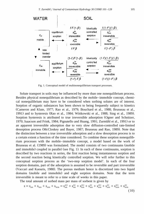
Fig. 1. Conceptual model of multinonequilibrium transport processes.
Solute transport in soils may be influenced by more than one nonequilibrium process.Besides physical nonequilibrium as described by the mobile–immobile concept, chemi-cal nonequilibrium may have to be considered when sorbing solutes are of interest.Sorption of organic substances has been shown to being frequently subject to kineticsŽCameron and Klute, 1977; Rao et al., 1979; Bouchard et al., 1988; Brusseau et al.,
. Ž .1991 and to hysteresis Rao et al., 1984; Wittkowski et al., 1988; Sing et al., 1989 .ŽSorption hysteresis is attributed to true irreversible adsorption Ogner and Schnitzer,
.1970; Isaacson and Frink, 1984; Pignatello and Huang, 1991; Zurmuhl et al., 1991 or to¨an apparent irreversible adsorption due to very slow diffusion-controlled rate-limited
Ž .desorption process McCloskey and Bayer, 1987; Brusseau and Rao, 1989 . Note thatthe distinction between a true irreversible adsorption and a slow desorption process is toa certain extent a function of the time considered. To combine these sorption nonequilib-rium processes with the mobile–immobile concept, a model based on the work of
Ž . ŽBrusseau et al. 1989 was formulated. The model consists of two continuums mobile. Ž .and immobile coupled in parallel see Fig. 1 . In each of these continuums, sorption is
described by two reactions in series, the first reaction being instantaneous sorption andthe second reaction being kinetically controlled sorption. We will refer further to thisconceptual sorption process as the ‘two-step sorption model’. In each of the foursorption domains, part of the adsorption is assumed to be reversible and part irreversibleŽ .Vaccari and Kaouris, 1988 . The porous medium hence is discretized into two liquid
Ž .domains mobile and immobile and eight sorption domains. Note that the termirreversible is meant to refer to a time scale of weeks in this paper.
The total amount of sorbed mass per mass of sorbent is given by
sss qs qs qs ss rev qs irr qs rev qs irr qs rev qs irr qs rev qs irrsm km sim kim sm sm km km sim sim kim kim
10Ž .
( )T. ZurmuhlrJournal of Contaminant Hydrology 30 1998 101–128¨106
w y3 x Ž .where s MM is the total sorbed mass divided by the mass of sorbent i.e., soil , ssmw y3 xand s MM are the masses of sorbate subject to instantaneous sorption in thesim
mobile and immobile region, respectively, divided by the total mass of sorbent, and skmw y3 xand s MM are the masses of sorbate subject to kinetic sorption in the mobile andkim
immobile region, respectively, divided by the total mass of sorbent. The superscripts revand irr indicate reversible or irreversible subdomains. At equilibrium, sorption in eachreversible subdomain is represented by the following linear equations:
s rev s fbFK c s rev s 1y f FbK cŽ .sm p m sim p im11Ž .rev revs s f 1yF bK c s s 1y f 1yF bK cŽ . Ž . Ž .km p m kim p im
w xwhere f y is the mass fraction of sorbent comprising the mobile region, fsu ru , Fmw x w xy is the fraction of sorbent for which sorption is instantaneous, and b y is thefraction of sorption sites for which sorption is reversible. Because the partitioning of thesoil water into a mobile and an immobile region should be regarded in a conceptual and
Ž Ž . Ž ..not strictly physical sense, F, b , k and k see Eqs. 17 and 18 are assumed to bead de
constant. Furthermore these parameters cannot be determined for the mobile andimmobile regions by independent experiments. For the irreversible domains, one has todistinguish whether adsorption or desorption takes place, and whether the concentrationin the reversible domains and in the water phase during adsorption exceeds any previousconcentration. The amount of mass in the irreversible domains at any time depends onthe maximum concentration in the corresponding reversible domain during the history ofthe experiment. If the concentration exceeds the previous concentration, adsorption takesplace and the reversible and irreversible domains are not distinguished anymore. If theconcentration decreases, the maximum concentration is stored and then sorption kineticsoccurs only between the different reversible sorption domains. The irreversible sorbedconcentration therefore can either be expressed by the corresponding reversible concen-
Ž .trations if the corresponding maximum concentration is exceeded or by the storedŽ .maximal concentration if the concentration is less then the maximum :
1yb°max rev maxs for s -si j i j i j
birr ~s s 12Ž .i j 1yb
rev rev maxs for s Gsi j i j i j¢ b
where smax is the maximum sorbed concentration in the reversible instantaneous ori,jŽ Ž . Ž ..kinetic mobile or immobile sorption domains, respectively, ig s,k ; jg m,im .
Assuming that f is constant for one-time step, sorption dynamics for each of thedifferent domains is described by the following set of equations:
Ec° m rev maxfFK for s Gsp sm smEs Etsm ~s 13Ž .EcEt m rev maxfFbK for s -s¢ p sm smEt
( )T. ZurmuhlrJournal of Contaminant Hydrology 30 1998 101–128¨ 107
Ec° im rev max1y f FK for s GsŽ . p sim simEs Etsim ~s 14Ž .EcEt im rev max1y f FbK for s -sŽ .¢ p sim simEt
1°) rev rev maxk f 1yF K c y s for s GsŽ .Es m p m km km kmkm ~ bs 15Ž .
Et) rev rev max¢k f 1yF bK c ys for s -sŽ .m p m km km km
1°) rev rev maxk 1y f 1yF K c y s for s GsŽ . Ž .Es im p im kim kim kimkim ~ bs 16Ž .
Et) rev rev max¢k 1y f 1yF bK c ys for s -sŽ . Ž .im p im kim kim kim
As different adsorption and desorption rate coefficients may exist, the following caseshave to be considered for the sorption rate constants in the mobile and immobile region,k ) and k ) :m im
k for f 1yF bK c Gs revŽ .ad p m km)k s 17Ž .m rev½k for f 1yF bK c -sŽ .de p m km
k for 1y f 1yF bK c Gs revŽ . Ž .ad p im kim)k s 18Ž .im rev½k for 1y f 1yF bK c -sŽ . Ž .de p im kim
w y1 x w y1 xwhere k T and k T are the adsorption and desorption rate constants,ad deŽ . Ž . Ž .respectively. Combining Eq. 6 with Eq. 13 to Eq. 16 leads to the final set of four
partial differential equations for the four unknowns c , c , s rev and s rev :m im km kim
)E u qr fFb K c E Ec EŽ .m sm p m m)s D u y Õ u c ya c ycŽ . Ž .m m m m m m imž /Et Ez Ez Ez
rk )
m revy f 1yF bK c ys 19Ž . Ž .p m km)bkm
)E u qr 1y f Fb K cŽ .Ž .im sim p im)sa c ycŽ .m im
Et
rk )
im revy 1y f 1yF bK c ysŽ . Ž . p im kim)bkim
20Ž .Es rev
km) revsk f 1yF bK c ys 21Ž . Ž .m p m km
Et
Es revkim
) revsk 1y f 1yF bK c ys 22Ž . Ž . Ž .im p im kimEt
( )T. ZurmuhlrJournal of Contaminant Hydrology 30 1998 101–128¨108
where b ) and b ) are given bysm,sim km,kim
1 for s rev Gsmaxsm ,sim sm ,sim
)b s 23Ž .rev maxsm ,sim ½b for s -ssm ,sim sm ,sim
b for s rev Gsmaxkm ,kim km ,kim
)b s 24Ž .rev maxkm ,kim ½ 1 for s -skm ,kim km ,kim
Ž . Ž . Ž . Ž . Ž . Ž . Ž .Eqs. 19 – 21 Eq. 22 together with Eqs. 17 , 18 , 23 and 24 in combination withŽ Ž .. Ž . Ž .the Richards equation Eq. 1 and the constitutive relationships, Eqs. 2 and 3 form
the basis to model unsaturated transient multinonequilibrium transport of solutes inporous media.
2.2. Numerical implementation
To complete the set of equations, initial and boundary conditions have to be given.For water flow the initial water content or matrix potential distribution in the region of
Ž . Ž .interest must be known. First Dirichlet and second-type Neumann boundary condi-tions can be specified for the upper and lower boundary. For the transport equations theinitial values for c , c , s rev and s rev have to be known throughout the region ofm im km kim
interest. For the upper boundary, a mixed form or third-type boundary is given.Ž .Following Celia et al. 1990 , the Richards equation is solved numerically using a fully
implicit finite-difference scheme with stable mass balance.The CDE and the multinonequilibrium model are solved numerically by modifying
Ž .the Euler–Lagrange method given by Yeh 1990 . For the multinonequilibrium modelthis method is possible only if the immobile water content, and therefore the fraction ofsorption sites in the mobile region, is assumed to be constant during the one-time step.
Ž . Ž .Eqs. 19 – 22 are discretized and combined. After some rearrangement the onlyŽ .unknowns in Eq. 19 are the new mobile concentrations at the different nodes. Thus Eq.
Ž .19 can be solved with a tridiagonal equation solver. The new mobile concentrations arethen used to successively calculate s rev, c and s rev . After computing the four differentkm im kim
Ž . Ž .concentrations the new immobile water content is calculated using Eq. 8 or Eq. 9 andthe fraction f tqD t is determined by f tqD t su tqD tru tqD t. Subsequently a mass ex-m
change between the mobile and immobile water phase and the mobile and immobileŽ .solid phase is carried out to guarantee an accurate mass balance see Appendix A . The
Fortran-code MUNETOS was written for numerical solution of the multinonequilibriumtransport model and tested against some analytical solutions for steady flow. The
Ž .software package CXTFIT Parker and van Genuchten, 1984 was used to obtain theŽ y1 .analytical solution for the transport of a linearly sorbing solute K s0.2 ml g whichp
Ž ) y1.is influenced either by physical nonequilibrium fsu rus0.4; a s0.05 h ormŽ y1 .chemical nonequilibrium Fs0.5, k sk s0.05 h . The flow velocity, Õ, was setad de
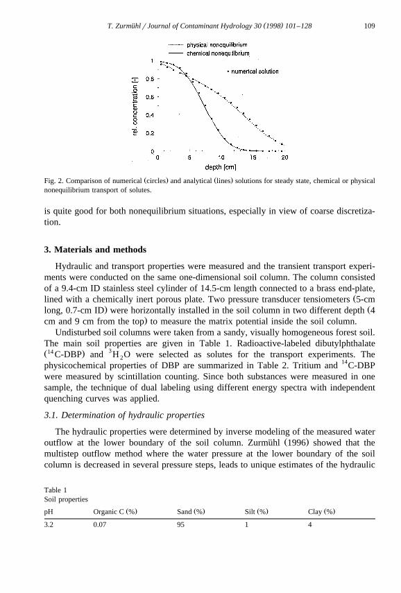
to 2.0 cm hy1 and a dispersivity ls0.5 cm was chosen. Fig. 2 shows the residentconcentrations in the soil profile after 5 h, calculated with the numerical model and theanalytical solution. Time and space were discretized by constant intervals D ts0.5 hand D zs1 cm, respectively. The agreement between analytical and numerical solution
( )T. ZurmuhlrJournal of Contaminant Hydrology 30 1998 101–128¨ 109
Ž . Ž .Fig. 2. Comparison of numerical circles and analytical lines solutions for steady state, chemical or physicalnonequilibrium transport of solutes.
is quite good for both nonequilibrium situations, especially in view of coarse discretiza-tion.
3. Materials and methods
Hydraulic and transport properties were measured and the transient transport experi-ments were conducted on the same one-dimensional soil column. The column consistedof a 9.4-cm ID stainless steel cylinder of 14.5-cm length connected to a brass end-plate,
Žlined with a chemically inert porous plate. Two pressure transducer tensiometers 5-cm. Žlong, 0.7-cm ID were horizontally installed in the soil column in two different depth 4
.cm and 9 cm from the top to measure the matrix potential inside the soil column.Undisturbed soil columns were taken from a sandy, visually homogeneous forest soil.
The main soil properties are given in Table 1. Radioactive-labeled dibutylphthalateŽ14 . 3C-DBP and H O were selected as solutes for the transport experiments. The2
physicochemical properties of DBP are summarized in Table 2. Tritium and 14C-DBPwere measured by scintillation counting. Since both substances were measured in onesample, the technique of dual labeling using different energy spectra with independentquenching curves was applied.
3.1. Determination of hydraulic properties
The hydraulic properties were determined by inverse modeling of the measured waterŽ .outflow at the lower boundary of the soil column. Zurmuhl 1996 showed that the¨
multistep outflow method where the water pressure at the lower boundary of the soilcolumn is decreased in several pressure steps, leads to unique estimates of the hydraulic
Table 1Soil properties
Ž . Ž . Ž . Ž .pH Organic C % Sand % Silt % Clay %
3.2 0.07 95 1 4
( )T. ZurmuhlrJournal of Contaminant Hydrology 30 1998 101–128¨110
Table 2Physicochemical properties of dibutylphthalate
y1 y1Ž . Ž . Ž .Molecular weight g mol Aqueous solubility mg l Log K Vapor pressure Pa, 258Cow
278.4 10.1 2.57 0.004
parameters. In order to measure hysteresis in the water retention curve, the pressure atthe lower boundary of the soil column was first decreased and then increased again toobtain drainage and imbibition curves.
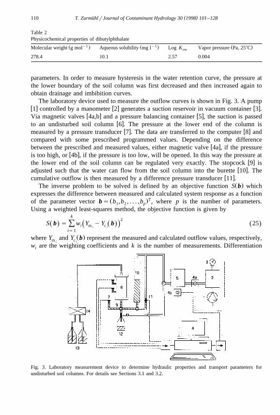
The laboratory device used to measure the outflow curves is shown in Fig. 3. A pumpw x w x w x1 controlled by a manometer 2 generates a suction reservoir in vacuum container 3 .
w x w xVia magnetic valves 4a,b and a pressure balancing container 5 , the suction is passedw xto an undisturbed soil column 6 . The pressure at the lower end of the column is
w x w xmeasured by a pressure transducer 7 . The data are transferred to the computer 8 andcompared with some prescribed programmed values. Depending on the difference
w xbetween the prescribed and measured values, either magnetic valve 4a , if the pressurew xis too high, or 4b , if the pressure is too low, will be opened. In this way the pressure at
w xthe lower end of the soil column can be regulated very exactly. The stopcock 9 isw xadjusted such that the water can flow from the soil column into the burette 10 . The
w xcumulative outflow is then measured by a difference pressure transducer 11 .Ž .The inverse problem to be solved is defined by an objective function S b which
expresses the difference between measured and calculated system response as a functionŽ .Tof the parameter vector bs b ,b , . . . ,b , where p is the number of parameters.1 2 p
Using a weighted least-squares method, the objective function is given byk
2S b s w Y yY b 25Ž . Ž . Ž .Ž .Ý i m ci i
is1
Ž .where Y and Y b represent the measured and calculated outflow values, respectively,m ci i
w are the weighting coefficients and k is the number of measurements. Differentiationi
Fig. 3. Laboratory measurement device to determine hydraulic properties and transport parameters forundisturbed soil columns. For details see Sections 3.1 and 3.2.
( )T. ZurmuhlrJournal of Contaminant Hydrology 30 1998 101–128¨ 111
of the objective function with respect to the parameter vector leads to a set of pnonlinear equations for the p unknown parameters, which has to be solved iteratively. AFortran program was written to solve this system of nonlinear equations with the methodof Levenberg–Marquardt. Details of the solution procedure can be found in Draper and
Ž . Ž .Smith 1981 and Kool and Parker 1988 . The value of u was independently measureds
by weighting the soil column after it was saturated at the end of the experiments. K s
was determined by measuring the saturated water flux for several hydraulic gradients.
3.2. Determination of transport properties
Ž .The laboratory equipment Fig. 3 was slightly modified to enable measurements ofw xthe transport parameters for the conservative tracer. The stopcock 9 was adjusted such
w xthat the solution leached from the soil column flowed into the sample bottle 12 . Thew x w xinput solution 13 was applied on the soil column with a syringe pump 14 and
dispersed over the soil surface by a teflon plate with 20 holes of diameter 0.5 mm. Thebreakthrough of solute was monitored as a function of time during steady flow. Aconstant water content throughout the soil column was achieved by adjusting thepressure at the lower boundary. The transport parameters were obtained by fitting the
Ž .CDE or MIM model to the measured breakthrough curves BTC’s using the softwareŽ .package CXTFIT Parker and van Genuchten, 1984 . The input solution consisted of a
0.01 M CaCl solution with and without 3H O as a conservative tracer. Breakthrough2 2
curves were measured for two different flow rates: qs2.6 cm hy1 and qs1.0 cm hy1.
3.3. Determination of sorption parameters
Sorption parameters for DBP were determined by batch experiments, measuringadsorption and desorption kinetics and adsorption and desorption isotherms. The sam-ples for all experiments were measured in triplicate.
3.3.1. Sorption isothermsFor the isotherms, six 14C-DBP-spiked DBP solutions having initial concentrations in
the range of 16 to 1040 mg ly1 were used in a background solution of 0.01 M CaCl .2
Additionally some NaN was added to the solutions to prevent microbiological degrada-3
tion. Sorption was initiated by mixing 4 g of dry soil with 15 ml of solution in 20 mlcentrifuge tubes. The slurries were shaken for 80 h to achieve equilibrium andcentrifuged at 2000 rpm for 15 min. A 5-ml sample of the supernatant of every slurrywas removed and analyzed by liquid scintillation. The amount of DBP sorbed by the soilwas calculated from the difference between the initial and final concentration of DBP insolution. On completion of the initial adsorption, 12 ml of the supernatant was removedand replaced by a DBP-free 0.01 M CaCl solution. The slurries were shaken for at least2
80 h and after centrifugation, an aliquot was removed for analysis. This procedure wasrepeated resulting in three successive desorption steps for every adsorption measurementpoint. To obtain the distribution coefficient K , adsorption isotherm data were fitted to ap
linear and a Freundlich-type adsorption isotherm. In order to determine the fraction ofŽreversible sorption, b , the data of all desorption isotherms were normalized Rao et al.,
( )T. ZurmuhlrJournal of Contaminant Hydrology 30 1998 101–128¨112
.1984 . Assuming a linear sorption isotherm, the sorbed equilibrium concentration, s ,de i j
after a desorption step is given by
s ss rev qs irr sK bc q 1yb s 26Ž . Ž .de de de p de adi j i j i j i j j
where c is the concentration in the water after a desorption step, s is the sorbedde adi j j
Ž .concentration after the adsorption step, i 1F iF3 is the number of the desorption stepŽ . Ž .for adsorption measurement point j 1F jF6 . Dividing Eq. 26 by s and recogniz-ad j
ing that s sK c yieldsad p adj j
s cde dei j i jsb q 1yb 27Ž . Ž .s cad adj j
where c is the concentration in the water after the adsorption step. Plotting s rsad de adj i j j
as a function of c rc gives an estimate for the parameter b.de adi j j
3.3.2. Sorption kineticsFor the adsorption and desorption kinetic experiments, the soil and the 0.01 M CaCl2
solution with an initial DBP concentration of 140 mg ly1 were equilibrated for differenttime durations. Concentrations in the solution and the soil were determined as describedabove. For the desorption experiment, a preliminary adsorption step was initiated.Assuming that during the experiments the total mass of solute is constant, the change ofthe concentration in the water is given by
Ec Essyr 28Ž .b
Et Et
w xwhere r smrV is the ratio of the mass m M of soil in the batch system, and thebw 3 xvolume V L of water during the experiment. Based on a linear sorption isotherm, the
two-step adsorption equation can be written as
Ec Es Es Ecs ksyr yr syr K F yr k K 1yF cys . 29Ž . Ž .b b b p b ad p k
Et Et Et Et
For the adsorption kinetics, the mass conservation equation reads
c VscVqms qms scVqmK Fcqms 30Ž .0 s k p k
w y3 xwhere c ML is the initial concentration in the water before the soil is added to the0Ž . Ž .experiment bottle. Combining Eqs. 29 and 30 gives the final equation for the kinetics
of the two-step adsorption model
Ec 1qr K cb p 0sk yc . 31Ž .ad ž /ž /Et 1qr K F 1qr Kb p b p
( )T. ZurmuhlrJournal of Contaminant Hydrology 30 1998 101–128¨ 113
For desorption kinetics, the irreversible fraction has to be considered, yielding
Ec Es rev qs irr qsr eÕqs irrŽ .k k s ssyr b
Et Et
Ecrevsyr K Fb yr k K 1yF bcys 32Ž . Ž .b p b de p k
Et
The mass balance for desorption reads
c VqmK yc V scVqmK Fbcqms rev qm 1yb K c 33Ž . Ž .Ž .ad p ad e p k p ad
w 3 xwhere V L is the volume of water, which is replaced by solute free 0.01 M CaCle 2
solution after the adsorption step and c is the concentration in the water after theadŽ . rev Ž .adsorption step. Solving Eq. 33 for s and inserting it into Eq. 32 , yields after somek
rearrangement
Ec 1qr K b 1yV rVqr K b cŽ .b p e b p adsk yc 34Ž .de ž / ž /Et 1qr K Fb 1qr K bb p b p
which describes the two-step desorption kinetics with irreversible adsorption for a batchŽ . Ž .experiment. The analytical solutions of Eqs. 31 and 34 are given in Appendix B.
3.4. Transient transport experiments
Transient transport experiments were carried out with a 0.01 M CaCl solution2
containing both 3H O together with 14C-DBP. The solutes were applied at the top of the2
soil column as finite pulse and the concentration in the effluent was measured as afunction of time for the given transient boundary conditions. The column was brought tohydraulic equilibrium at the start of the experiment.
4. Results and discussion
First the results of the parameter determination are discussed. Subsequently, mea-sured transient water and solute transport are compared with prediction using either theequilibrium or the multinonequilibrium model.
4.1. Hydraulic properties
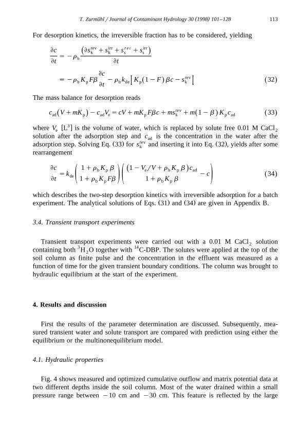
Fig. 4 shows measured and optimized cumulative outflow and matrix potential data attwo different depths inside the soil column. Most of the water drained within a smallpressure range between y10 cm and y30 cm. This feature is reflected by the large
( )T. ZurmuhlrJournal of Contaminant Hydrology 30 1998 101–128¨114
Ž . Ž . Ž .Fig. 4. Measured open symbols and optimized cumulative outflow bottom and matrix potential top dataŽ . Ž .for drying and wetting, including hysteresis solid line or only drying dotted line . The pressure at the lower
Ž .boundary is given as the dashed line bottom .
value of the parameter n, as can be seen from Table 3. Hysteresis can be recognized bycomparing the cumulative outflow values during the drainage and wetting cycles atequal pressure of the lower boundary. During the parameter determination, u and Ks s
were fixed and a , a , n, u and t were optimized simultaneously. Different initialw d r
parameter guesses lead to nearly the same parameter values indicating a global mini-mum. The fitted outflow and inflow data agree reasonably well with the measured data.However, some systematic deviations occur. These deviations are likely due in part to
Ž .the hysteresis model of Kool and Parker 1987 , which introduces only one additionalparameter to describe the main wetting and drying curves. A slightly better fit isachieved when only the drainage outflow curve is optimized. Another discrepancy canbe observed between the measured water pressures and the outflow values. Whereas the
Žtensiometers indicate hydraulic equilibrium, water is still leaving the soil column e.g.,
Table 3Hydraulic parameters from multistep outflow experiment
y1 y1 y1Ž . Ž . Ž .a cm a cm n u u K cm h tw d r s s
0.0568 0.0420 4.44 0.165 0.387 10.4 0.358"0.0004 "0.0002 "0.0073 "0.002 y y "0.041
( )T. ZurmuhlrJournal of Contaminant Hydrology 30 1998 101–128¨ 115
.between ts35 h and ts55 h . This discrepancy can be explained by a dynamicŽ . Ž .component of the water retention curve. Smiles et al. 1971 and Vachaud et al. 1972
Ž .demonstrated that a transient u c curve obtained by rapidly changing the matrixŽ .potential, i.e., EcrEt40, at one side of a soil column, may be different from a u c
curve obtained from static measurements, i.e., EcrEtf0. They observed that transientwater retention curves always showed higher water contents than the static curve for thesame pressure and that this effect is most pronounced in the range with the steepest
Ž .slope of the u c curve. These findings are in agreement with our measurements. Thecumulative outflow is too low at the beginning of the pressure step, leading to a too highwater content in the soil column. Furthermore the effect is limited to a pressure rangefrom csy10 cm to csy20 cm in which u changes significantly.
4.2. Transport parameters
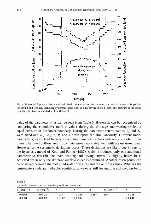
Ž .To determine transport parameters, the equilibrium CDE and the nonequilibriumŽ . 3MIM models were fitted to measured breakthrough curves of H O for two different2
flow velocities. Note that the only nonequilibrium process for 3H O can be the physical2
mobile–immobile concept, because the tracer does not interact with the soil matrix. TheŽ . ) Ž .parameters Õ and D CDE and additionally a and fsu ru MIM were optimizedm
independently for both flow velocities. Since the model considers l and a ) asconstants, only mean values for these parameters were calculated. The fitting wassubsequently repeated with l and a ) fixed at their mean values. The results are shownin Fig. 5 and the transport parameters are given in Table 4. Tailing of the experimentalBTC’s is obvious for both flow velocities close to the peak maximum and when theconcentration approaches zero. As expected this tailing can be described with the MIM
Ž .model but not with CDE. To obtain u or g from the value of f using Eq. 8 or Eq.imŽ .9 , the water content during the BTC experiments has to be known. This value can be
Ž . Ž .calculated 1 by usqrÕ with the values from Table 4 or 2 by determining the waterŽ . Ž .content from K u assuming gravity flow, i.e., K u sq. The two methods yield water
contents of 0.234 and 0.261 for qs2.63 cm hy1, and 0.207 and 0.235 for qs1.02 cm
Ž . 3Fig. 5. Measured solid symbols and optimized breakthrough curves for H O at two different flow velocities.2
The measured data were fitted with the CDE or the mobile–immobile model. l and a ) for the MIM modelwere fixed at the same value for both flow velocities.
( )T. ZurmuhlrJournal of Contaminant Hydrology 30 1998 101–128¨116
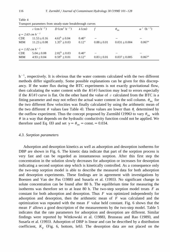
Table 4Transport parameters from steady-state breakthrough curves
y1 2 y1 ) y1Ž . Ž . Ž . Ž .Õ cm h D cm h l cm f u a him
y 1qs 2.63 cm hb aCDE 11.53"0.16 4.61 "0.04 0.40 y y yb a aMIM 11.23"0.08 1.35 "0.03 0.12 0.88"0.01 0.031"0.004 0.067
y 1qs1.02 cm hb aCDE 5.04"0.08 2.02 "0.03 0.40 y y yb a aMIM 4.93"0.04 0.59 "0.01 0.12 0.83"0.01 0.037"0.005 0.067
hy1, respectively. It is obvious that the water contents calculated with the two differentmethods differ significantly. Some possible explanations can be given for this discrep-ancy. If the water flux during the BTC experiments is not exactly gravitational flow,
Ž .then calculating the water content with the K u function may lead to errors especiallyŽ .if the K u curve is flat. On the other hand the value of Õ calculated from the BTC is a
fitting parameter and may not reflect the actual water content in the soil column. u forim
the two different flow velocities was finally calculated by using the arithmetic mean ofŽ .the two different u values see Table 4 . These values are lower than u determined byr
Ž .the outflow experiment. Thus the concept proposed by Zurmuhl 1996 to vary u with¨ im
u in a way that depends on the hydraulic conductivity function could not be applied. WeŽ .therefore used Eq. 8 and set gsu sconst.s0.034.im
4.3. Sorption parameters
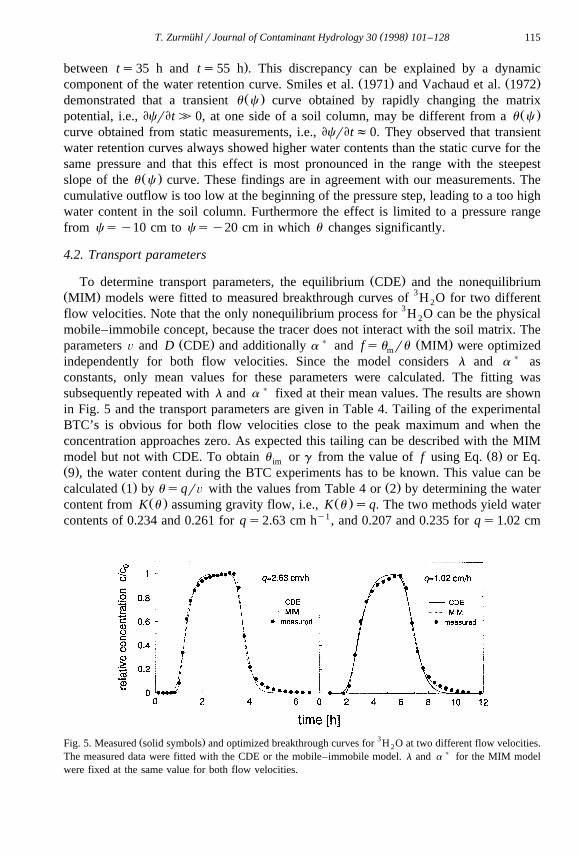
Adsorption and desorption kinetics as well as adsorption and desorption isotherms forDBP are shown in Fig. 6. The kinetic data indicate that part of the sorption process isvery fast and can be regarded as instantaneous sorption. After this first step theconcentration in the solution slowly decreases for adsorption or increases for desorptionindicating a second sorption step which is kinetically controlled. As a consequence onlythe two-step sorption model is able to describe the measured data for both adsorptionand desorption experiments. These findings are in agreement with investigations by
Ž . Ž .Boesten and Van der Pas 1988 and Susarla et al. 1993 . No significant change insolute concentration can be found after 80 h. The equilibrium time for measuring theisotherms was therefore set to at least 80 h. The two-step sorption model treats F asconstant for both adsorption and desorption. Thus F was optimized independently foradsorption and desorption, then the arithmetic mean of F was calculated and theoptimization was repeated with the mean F value held constant. Fig. 6 shows that themean F allows a good description of the measurements by the two-step model. Table 5indicates that the rate parameters for adsorption and desorption are different. Similar
Ž . Ž .findings were reported by Wittkowski et al. 1988 , Brusseau and Rao 1989 , andŽ .Susarla et al. 1993 . Adsorption of DBP is linear and can be described by a distribution
Ž .coefficient, K Fig. 6, bottom, left . The desorption data are not placed on thep
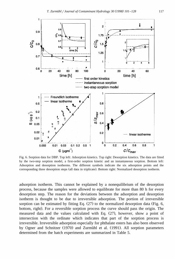
( )T. ZurmuhlrJournal of Contaminant Hydrology 30 1998 101–128¨ 117
Fig. 6. Sorption data for DBP. Top left: Adsorption kinetics. Top right: Desorption kinetics. The data are fittedby the two-step sorption model, a first-order sorption kinetic and an instantaneous sorption. Bottom left:Adsorption and desorption isotherms. The different symbols indicate the six adsorption points and the
Ž .corresponding three desorption steps all data in triplicate . Bottom right: Normalized desorption isotherm.
adsorption isotherm. This cannot be explained by a nonequilibrium of the desorptionprocess, because the samples were allowed to equilibrate for more than 80 h for everydesorption step. The reason for the deviations between the adsorption and desorptionisotherm is thought to be due to irreversible adsorption. The portion of irreversible
Ž . Žsorption can be estimated by fitting Eq. 27 to the normalized desorption data Fig. 6,.bottom, right . For a reversible sorption process the curve should pass the origin. The
Ž .measured data and the values calculated with Eq. 27 , however, show a point ofintersection with the ordinate which indicates that part of the sorption process isirreversible. Irreversible adsorption especially for phthalate esters has also been observed
Ž . Ž .by Ogner and Schnitzer 1970 and Zurmuhl et al. 1991 . All sorption parameters¨determined from the batch experiments are summarized in Table 5.
( )T. ZurmuhlrJournal of Contaminant Hydrology 30 1998 101–128¨118
Table 5Sorption parameters from batch experiments
y1 y1 y1Ž . Ž . Ž .K ml g F k h k h bp ad de
1.49"0.02 0.52 0.031"0.018 0.069"0.060 0.67"0.01
4.4. Transient water flow
In the next part the results of the transient water and solute transport experiments willbe discussed together with the predictions of the equilibrium and the nonequilibriummodel using the independently determined parameters. No calibration or parameterfitting is used to calculate the model outputs, unless mentioned explicitly.
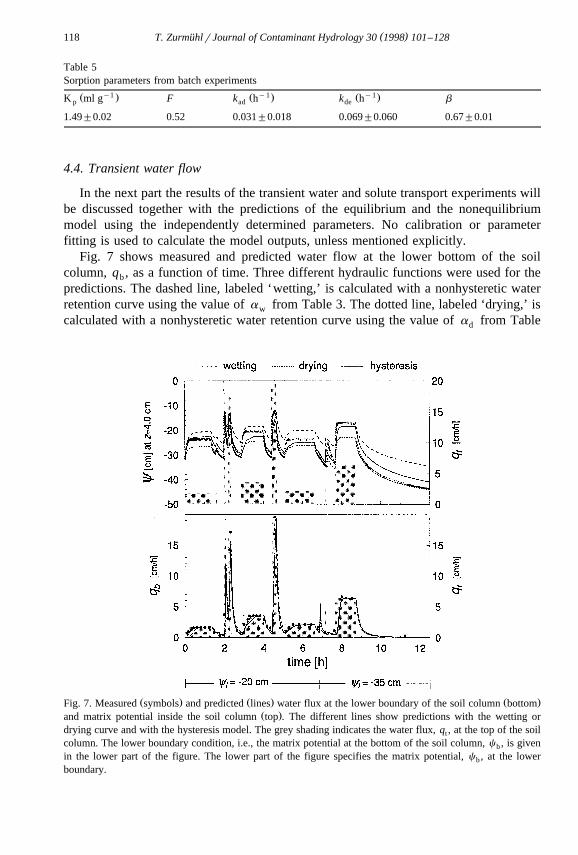
Fig. 7 shows measured and predicted water flow at the lower bottom of the soilcolumn, q , as a function of time. Three different hydraulic functions were used for theb
predictions. The dashed line, labeled ‘wetting,’ is calculated with a nonhysteretic waterretention curve using the value of a from Table 3. The dotted line, labeled ‘drying,’ isw
calculated with a nonhysteretic water retention curve using the value of a from Tabled
Ž . Ž . Ž .Fig. 7. Measured symbols and predicted lines water flux at the lower boundary of the soil column bottomŽ .and matrix potential inside the soil column top . The different lines show predictions with the wetting or
drying curve and with the hysteresis model. The grey shading indicates the water flux, q , at the top of the soilt
column. The lower boundary condition, i.e., the matrix potential at the bottom of the soil column, c , is givenb
in the lower part of the figure. The lower part of the figure specifies the matrix potential, c , at the lowerb
boundary.
( )T. ZurmuhlrJournal of Contaminant Hydrology 30 1998 101–128¨ 119
Ž .3. The third line is calculated using the hysteresis model of Kool and Parker 1987 witha and a from Table 3. The water flux is nearly perfectly predicted with all of thew d
different calculations. The outflow therefore is insensitive on hysteretic water retentioncurves for the chosen boundary conditions. This low sensitivity can be explained bycomparing the outflow with the upper boundary condition. A given flux will adjust awater content inside the soil which allows the drainage of the infiltrating water to thebottom of the soil. Thus, a quasi steady-state water flux is rapidly established. Thisconstant water flux is influenced only by the flux across the upper boundary and not bythe form of the water retention curve.
The results for the matrix potential inside the soil column at 4-cm depth from the topare shown in the upper part of Fig. 7. The measured data follow changes in the boundaryconditions. During infiltration the potentials rapidly increase whereas during redistribu-tion, with no inflow at the top of the column, the potentials only decrease slowly due tothe decrease in hydraulic conductivity. None of the predictions agrees well with themeasured data for the total time considered. The prediction with hysteresis shows thesmallest overall deviation between measurement and prediction. The nonhystereticsimulations with the wetting curve poorly matches the measured matrix potentials duringredistribution periods but yield good agreement with the measured data during infiltra-tion events. On the other hand, the calculations with the drying curve cannot predict thematrix potential during infiltration but will lead to an excellent agreement betweenmeasurements and predictions for phases of redistribution. This phenomenon is mostpronounced at ts7.8 h to ts12.5 h. Therefore, hysteresis should be considered formodeling transient water flow to get reliable predictions of matrix head in soils.
Ž .However, the hysteresis model of Kool and Parker 1987 cannot describe the observedhysteretic behaviour since the scanning loops between the main drying and imbibitioncurves are too smooth. A better prediction of the measured data probably could byobtained if the scanning paths go directly from the point of reflection to the mainimbibition or drying branches.
4.5. Transient solute transport
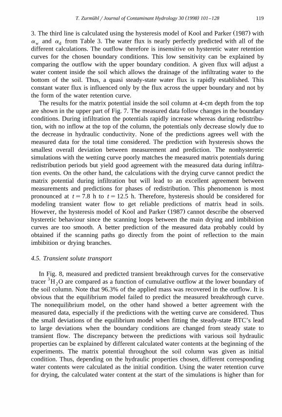
In Fig. 8, measured and predicted transient breakthrough curves for the conservativetracer 3H O are compared as a function of cumulative outflow at the lower boundary of2
the soil column. Note that 96.3% of the applied mass was recovered in the outflow. It isobvious that the equilibrium model failed to predict the measured breakthrough curve.The nonequilibrium model, on the other hand showed a better agreement with themeasured data, especially if the predictions with the wetting curve are considered. Thusthe small deviations of the equilibrium model when fitting the steady-state BTC’s leadto large deviations when the boundary conditions are changed from steady state totransient flow. The discrepancy between the predictions with various soil hydraulicproperties can be explained by different calculated water contents at the beginning of theexperiments. The matrix potential throughout the soil column was given as initialcondition. Thus, depending on the hydraulic properties chosen, different correspondingwater contents were calculated as the initial condition. Using the water retention curvefor drying, the calculated water content at the start of the simulations is higher than for
( )T. ZurmuhlrJournal of Contaminant Hydrology 30 1998 101–128¨120
Ž .Fig. 8. Measured filled circles and predicted transient tracer BTC using the nonequilibrium mobile–immobileŽ . Ž .top and the equilibrium bottom models. The different lines show predictions with wetting or drying curveand with the hysteresis model. The grey shading indicates the water flux, q , at the top of the soil column.t
the wetting curve. The water front therefore moves somewhat faster when using thedrying curve, leading to slightly higher values of cumulative outflow at the same time.These small differences can only hardly be seen in Fig. 7. Solute transport is controlled
Ž .by the mean mobile pore water velocity which is given by the infiltration rate dividedŽ . Ž .by the mobile water content. Since the K u -function is assumed not to be hysteretic,
the water content in the soil column behind the different infiltration fronts will be nearlythe same for drying and wetting water retention curves. As the infiltration rate is also thesame for drying and wetting, solute transport is not affected by the different hydraulicproperties. If these findings are related to the different cumulative outflow values, then itbecomes comprehensible that calculations with the wetting curve lead to an earlierbreakthrough if the concentration is depicted as a function of cumulative outflow.
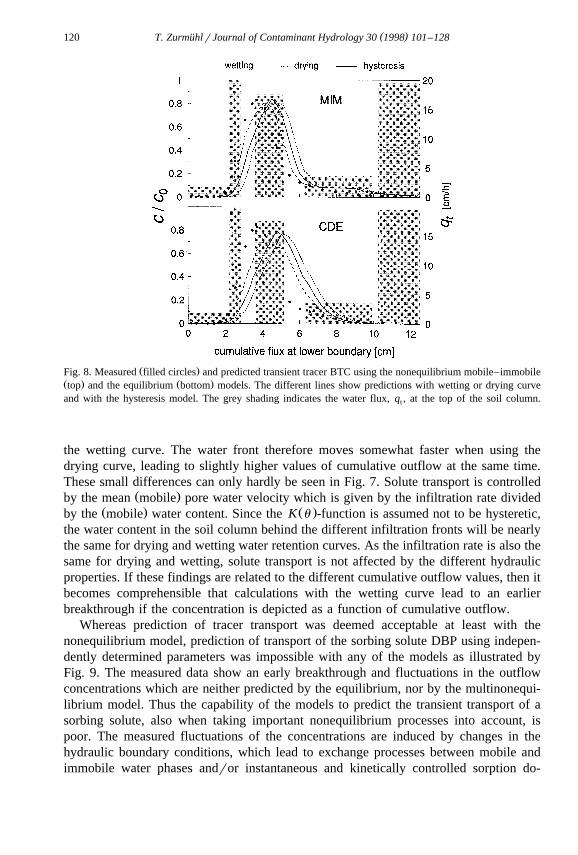
Whereas prediction of tracer transport was deemed acceptable at least with thenonequilibrium model, prediction of transport of the sorbing solute DBP using indepen-dently determined parameters was impossible with any of the models as illustrated byFig. 9. The measured data show an early breakthrough and fluctuations in the outflowconcentrations which are neither predicted by the equilibrium, nor by the multinonequi-librium model. Thus the capability of the models to predict the transient transport of asorbing solute, also when taking important nonequilibrium processes into account, ispoor. The measured fluctuations of the concentrations are induced by changes in thehydraulic boundary conditions, which lead to exchange processes between mobile andimmobile water phases andror instantaneous and kinetically controlled sorption do-
( )T. ZurmuhlrJournal of Contaminant Hydrology 30 1998 101–128¨ 121
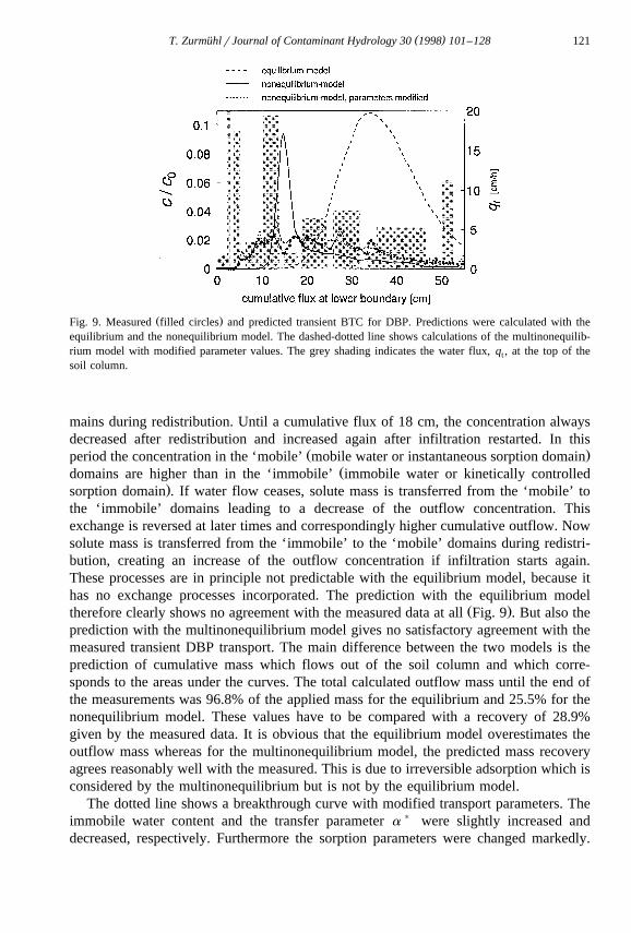
Ž .Fig. 9. Measured filled circles and predicted transient BTC for DBP. Predictions were calculated with theequilibrium and the nonequilibrium model. The dashed-dotted line shows calculations of the multinonequilib-rium model with modified parameter values. The grey shading indicates the water flux, q , at the top of thet
soil column.
mains during redistribution. Until a cumulative flux of 18 cm, the concentration alwaysdecreased after redistribution and increased again after infiltration restarted. In this
Ž .period the concentration in the ‘mobile’ mobile water or instantaneous sorption domainŽdomains are higher than in the ‘immobile’ immobile water or kinetically controlled
.sorption domain . If water flow ceases, solute mass is transferred from the ‘mobile’ tothe ‘immobile’ domains leading to a decrease of the outflow concentration. Thisexchange is reversed at later times and correspondingly higher cumulative outflow. Nowsolute mass is transferred from the ‘immobile’ to the ‘mobile’ domains during redistri-bution, creating an increase of the outflow concentration if infiltration starts again.These processes are in principle not predictable with the equilibrium model, because ithas no exchange processes incorporated. The prediction with the equilibrium model
Ž .therefore clearly shows no agreement with the measured data at all Fig. 9 . But also theprediction with the multinonequilibrium model gives no satisfactory agreement with themeasured transient DBP transport. The main difference between the two models is theprediction of cumulative mass which flows out of the soil column and which corre-sponds to the areas under the curves. The total calculated outflow mass until the end ofthe measurements was 96.8% of the applied mass for the equilibrium and 25.5% for thenonequilibrium model. These values have to be compared with a recovery of 28.9%given by the measured data. It is obvious that the equilibrium model overestimates theoutflow mass whereas for the multinonequilibrium model, the predicted mass recoveryagrees reasonably well with the measured. This is due to irreversible adsorption which isconsidered by the multinonequilibrium but is not by the equilibrium model.
The dotted line shows a breakthrough curve with modified transport parameters. Theimmobile water content and the transfer parameter a ) were slightly increased anddecreased, respectively. Furthermore the sorption parameters were changed markedly.
( )T. ZurmuhlrJournal of Contaminant Hydrology 30 1998 101–128¨122
The fraction of instantaneous sorption, F, was decreased from its originating valueFs0.52 to Fs0.1 and the adsorption and desorption rate parameters were increasedfrom k s0.031 to k s1.0 and k s0.069 to k s1.5. With these modifiedad ad de de
parameters, a much better agreement between measurements and model calculationscould be obtained. Note that no optimization algorithm was used and that the parameterswere modified by the method of trial-and-error. The early breakthrough and the massexchange processes can now be reproduced by the simulations. The low value of Findicates that the sorption parameters obtained from the batch experiments are of limitedapplicability to model sorption behaviour in an undisturbed soil under transient flowconditions. Whereas all possible sorption site are accessible during batch experimentsdue to shaking of the soil suspension, in flow experiments part of the sorption sites maybe accessible only by diffusion. Thus especially for high flow velocities, this diffusion-limited sorption capacity leads to an early breakthrough as can be observed by themeasured data. Furthermore the model assumption of a homogeneous distribution oforganic carbon in the soil may not be fulfilled. A negative correlation of pore size andorganic carbon content will also lead to an early breakthrough of the sorbing solute.
5. Summary and conclusions
In this work the capability of an equilibrium and a multi nonequilibrium convection-dispersion-model to predict transient movement of a conservative and a sorbing solute inan undisturbed soil column was investigated.
The multistep outflow measurements, as well as the transient experiments, showedthat the water retention curve is hysteretic. The data indicated, however, that the
Ž .hysteresis model of Kool and Parker 1987 is only partly successful to predict thematrix potential in the soil column. The measured data were best modeled using thewetting curve during infiltration and the drying curve during drainage or redistribution.
The transport of the tracer could be predicted more or less satisfactorily using themultinonequilibrium model. The equilibrium model calculated a breakthrough whichlagged behind the measured data. It is shown that both physical and chemical nonequi-librium processes are involved in the transport of the sorbing compound. Modelsassuming equilibrium sorption reactions and the infiltrating water to completely replacethe ‘old’ water in the soil are therefore not suitable to predict the observed transportpatterns in a homogeneous medium. The multinonequilibrium model also failed topredict the measured transient BTC using the independently determined input parame-ters. The measured data showed an earlier breakthrough and more fluctuations in theoutflow concentration caused by exchange processes between domains of differentmobility. A calibration of the multinonequilibrium model, however, seemed possible.Changing particularly, the sorption parameters led to model calculations which were ingood agreement with the measured data. It is concluded that sorption parameters frombatch experiments may not always be appropriate to model sorption phenomena inundisturbed soils with high water flow rates. The accessibility of possible sorption sitesmay become diffusion-controlled and then can not be compared with batch experiments.This has implications especially on common methods to predict solute transport in the
( )T. ZurmuhlrJournal of Contaminant Hydrology 30 1998 101–128¨ 123
field using batch sorption parameters. If the heterogeneity of the organic carbondistribution in the field is neglected and the reduced accessibility of sorption sites is notconsidered in the model, then the prediction of solute transport in the field may lead togross errors compared to the actual solute transport.
Acknowledgements
Ž .This work was funded by the Deutsche Forschungsgemeinschaft DFG undercontract number He 482r22-1. I express my appreciation to R. Herrmann from theDepartment of Hydrology at the University of Bayreuth for giving me the opportunity toperform the laboratory experiments at his institute and to W. Durner and K. Roth forfruitful discussions.
Appendix A
Solving the multinonequilibrium model using a modified Euler–Lagrange methodrequires the mobile water content, u , and the fraction of sorbent in contact with theim
mobile water, f , to be constant for one-time step. Because u and f may have changedim
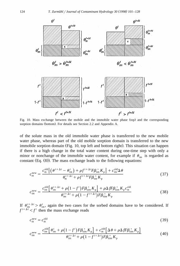
during the time step, a mass exchange between the new mobile and the immobile waterphase and between the four reversible sorption domains has to be carried out. Thechange of concentration for the instantaneous reacting sorption domains are given inconjunction with the exchange of the water phase concentration. As can be seen fromFig. 10, four cases have to be considered.
Ž .First, if the immobile water content decreases Fig. 10, top left and f increasesŽ . Ž tqD t t tqD t.during one-time step, Fig. 10, bottom left u -u n f then part of the soluteim im
Ž .mass marked by ‘x’ , actually attached to the old immobile region, is transferred to theŽ .new mobile domain and part of the sorbed mass marked by ‘x’ in the old immobile,
Ž t.instantaneous and kinetic sorption domains 1y f is transferred to the new correspond-Ž tqD t.ing mobile domains f . In this case, the mass balance for the mobile and immobile
water phases and the corresponding instantaneous reacting sorption domains before andafter the mass exchange yields:
old tqD t t t ) old )c u yu qr f Fb K qc DuqrD fFb KŽ .m im sm p im sm pnewc s 35Ž .m tqD t tqD t )u qr f Fb Km sm p
cnew scold 36Ž .im im
where
< t tqD t <Dus u yuim im
< tqD t t <D fs f y f
and cold,new, are the mobile and immobile concentration before and after the massm,im
exchange, respectively. If u tqD t -u t n f tqD t - f t, then the situation arises where partim im
( )T. ZurmuhlrJournal of Contaminant Hydrology 30 1998 101–128¨124
Ž .Fig. 10. Mass exchange between the mobile and the immobile water phase top and the correspondingŽ .sorption domains bottom . For details see Section 2.2 and Appendix A.
of the solute mass in the old immobile water phase is transferred to the new mobilewater phase, whereas part of the old mobile sorption domain is transferred to the new
Ž .immobile sorption domain Fig. 10, top left and bottom right . This situation can happenif there is a high change in the total water content during one-time step with only aminor or nonchange of the immobile water content, for example if u is regarded asim
Ž Ž ..constant Eq. 8 . The mass exchange leads to the following equations:
old tqD t t tqD t ) oldc u yu qr f Fb K qc DuŽ .m im sm p imnewc s 37Ž .m tqD t tqD t )u qr f Fb Km sm p
old tqD t t ) ) oldc u qr 1y f Fb K qrD fFb K cŽ .im im sim p sim p mnewc s 38Ž .im tqD t tqD t )u qr 1y f Fb KŽ .im sim p
If u tqD t )u t , again the two cases for the sorbed domains have to be considered. Ifim im
f tqD t - f t then the mass exchange reads
cnew scold 39Ž .m m
old t t ) old )c u qr 1y f Fb K qc DuqrD fFb KŽ .im im sim p m sim pnewc s 40Ž .im tqD t tqD t )u qr 1y f Fb KŽ .im sim p
( )T. ZurmuhlrJournal of Contaminant Hydrology 30 1998 101–128¨ 125
and for the case f tqD t ) f t one gets:
old tqD t t ) ) oldc u qr f Fb K qrD fFb K cm m sm p sm p imnewc s 41Ž .m tqD t tqD t )u qr f Fb Km sm p
old t tqD t ) oldc u qr 1y f Fb K qc DuŽ .im im sim p mnewc s 42Ž .im tqD t tqD t )u qr 1y f Fb KŽ .im sim p
For the kinetically controlled reversible sorption domains, only two cases have to beconsidered. If f tqD t - f t, then the mass exchange is given by
D fnew old olds ss q s 43Ž .km km kimt1y f
and
1y f tqD tnew olds s s 44Ž .kim kimt1y f
tqD t t Ž . Ž .For situations where f - f , Eqs. 43 and 44 can be used with all subscripts kmreplaced by kim and vice versa and with 1y f tqD t and 1y f t replaced by f tqD t and f t,respectively. The mass exchange between the irreversible domains is carried out in thesame way as for the reversible domains.
Appendix B
Ž . Ž .Eqs. 31 and 34 can be written in a general form with coefficients A and B as
EcsAcqB 45Ž .
Et
with the solution
c t sexp tA c qBrA yBrA 46Ž . Ž . Ž . Ž .b
where c is the concentration at the begin of the batch experiment. As the fraction F ofb
the soil reacts instantaneously with the solute in the water, the concentration at thebeginning of the adsorption study has to be calculated assuming that the instantaneousfraction of the soil is in equilibrium with the concentration in the water and that thekinetic fraction is free of sorbent:
c Vsc Vqm s qs sc VqmK Fc ´c sc r 1qr K F 47Ž . Ž .Ž .0 b s k b p b b 0 b p
For the desorption process, the concentration at the start of the desorption kinetics canbe calculated in an analogous way and is given by
c 1yV rVqr K FbŽ .ad e b pc s 48Ž .b 1qr K Fbb p
( )T. ZurmuhlrJournal of Contaminant Hydrology 30 1998 101–128¨126
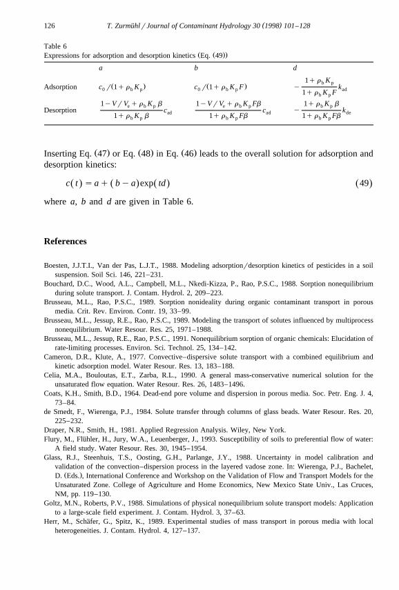
Table 6Ž Ž ..Expressions for adsorption and desorption kinetics Eq. 49
a b d
1q r Kb pŽ . Ž .Adsorption c r 1q r K c r 1q r K F y k0 b p 0 b p ad1q r K Fb p
1yVr V q r K b 1yVr V q r K Fb 1q r K be b p e b p b pDesorption c c y kad ad de1q r K b 1q r K Fb 1q r K Fbb p b p b p
Ž . Ž . Ž .Inserting Eq. 47 or Eq. 48 in Eq. 46 leads to the overall solution for adsorption anddesorption kinetics:
c t saq bya exp td 49Ž . Ž . Ž . Ž .
where a, b and d are given in Table 6.
References
Boesten, J.J.T.I., Van der Pas, L.J.T., 1988. Modeling adsorptionrdesorption kinetics of pesticides in a soilsuspension. Soil Sci. 146, 221–231.
Bouchard, D.C., Wood, A.L., Campbell, M.L., Nkedi-Kizza, P., Rao, P.S.C., 1988. Sorption nonequilibriumduring solute transport. J. Contam. Hydrol. 2, 209–223.
Brusseau, M.L., Rao, P.S.C., 1989. Sorption nonideality during organic contaminant transport in porousmedia. Crit. Rev. Environ. Contr. 19, 33–99.
Brusseau, M.L., Jessup, R.E., Rao, P.S.C., 1989. Modeling the transport of solutes influenced by multiprocessnonequilibrium. Water Resour. Res. 25, 1971–1988.
Brusseau, M.L., Jessup, R.E., Rao, P.S.C., 1991. Nonequilibrium sorption of organic chemicals: Elucidation ofrate-limiting processes. Environ. Sci. Technol. 25, 134–142.
Cameron, D.R., Klute, A., 1977. Convective–dispersive solute transport with a combined equilibrium andkinetic adsorption model. Water Resour. Res. 13, 183–188.
Celia, M.A., Bouloutas, E.T., Zarba, R.L., 1990. A general mass-conservative numerical solution for theunsaturated flow equation. Water Resour. Res. 26, 1483–1496.
Coats, K.H., Smith, B.D., 1964. Dead-end pore volume and dispersion in porous media. Soc. Petr. Eng. J. 4,73–84.
de Smedt, F., Wierenga, P.J., 1984. Solute transfer through columns of glass beads. Water Resour. Res. 20,225–232.
Draper, N.R., Smith, H., 1981. Applied Regression Analysis. Wiley, New York.Flury, M., Fluhler, H., Jury, W.A., Leuenberger, J., 1993. Susceptibility of soils to preferential flow of water:¨
A field study. Water Resour. Res. 30, 1945–1954.Glass, R.J., Steenhuis, T.S., Oosting, G.H., Parlange, J.Y., 1988. Uncertainty in model calibration and
validation of the convection–dispersion process in the layered vadose zone. In: Wierenga, P.J., Bachelet,Ž .D. Eds. , International Conference and Workshop on the Validation of Flow and Transport Models for the
Unsaturated Zone. College of Agriculture and Home Economics, New Mexico State Univ., Las Cruces,NM, pp. 119–130.
Goltz, M.N., Roberts, P.V., 1988. Simulations of physical nonequilibrium solute transport models: Applicationto a large-scale field experiment. J. Contam. Hydrol. 3, 37–63.
Herr, M., Schafer, G., Spitz, K., 1989. Experimental studies of mass transport in porous media with local¨heterogeneities. J. Contam. Hydrol. 4, 127–137.
( )T. ZurmuhlrJournal of Contaminant Hydrology 30 1998 101–128¨ 127
Hillel, D., 1991. Research in soil physics: A review. Soil Sci. 151, 30–34.Isaacson, P.J., Frink, C.R., 1984. Nonreversible sorption of phenolic compounds by sediment fractions: Role
of sediment organic matter. Environ. Sci. Technol. 18, 43–48.Jones, R.L., Rao, P.S.C., 1988. Reflections on validation and applications of unsaturated zone models. In:
Ž .Wierenga, P.J., Bachelet, D. Eds. , International Conference and Workshop on the Validation of Flow andTransport Models for the Unsaturated Zone. College of Agriculture and Home Economics, New MexicoState Univ., Las Cruces, NM, pp. 197–205.
Khan, A.U.H., Jury, W.A., 1990. A laboratory test of the dispersion scale effect. J. Contam. Hydrol. 5,119–132.
Kool, J.B., Parker, J.C., 1987. Development and evaluation of closed-form expressions for hysteretic soilhydraulic properties. Water Resour. Res. 23, 105–114.
Kool, J.B., Parker, J.C., 1988. Analysis of the inverse problem for transient unsaturated flow. Water Resour.Res. 24, 817–830.
McCloskey, W.B., Bayer, D.E., 1987. Thermodynamics of fluridone adsorption and desorption on threeCalifornia soils. Soil Sci. Soc. Am. J. 51, 605–612.
Mualem, Y., 1976. A new model for predicting the hydraulic conductivity of unsaturated porous media. WaterResour. Res. 12, 513–522.
Nielsen, D.R., van Genuchten, M.T., Biggar, J.W., 1986. Water flow and solute transport processes in theunsaturated zone. Water Resour. Res. 22, 895–1085.
Nkedi-Kizza, P., Biggar, J.W., van Genuchten, M.T., Wierenga, P.J., Selim, H.M., Davidson, J.M., Nielsen,D.R., 1983. Modeling tritium and chloride-36 transport through an aggregated oxisol. Water Resour. Res.19, 691–700.
Ogner, G., Schnitzer, M., 1970. Humic substances: Fulvic acid–dialkyl phthalate complexes and their role inpollution. Science 170, 317–318.
Parker, J.C., van Genuchten, M.T., 1984. Determining transport parameters from laboratory and field tracerexperiments. Bulletin 84-3, Virginia Agricultural Experiment Station, VA.
Pennell, K.D., Hornsby, A.G., Jessup, R.E., Rao, P.S.C., 1990. Evaluation of five simulation models forpredicting aldicarb and bromide behaviour under field conditions. Water Resour. Res. 26, 2679–2693.
Pignatello, J.J., Huang, L.Q., 1991. Sorptive reversibility of atrazine and metachlor residues in field soilsamples. J. Environ. Qual. 20, 222–228.
Rao, P.S.C., Davidson, J.M., Jessup, R.E., Selim, H.M., 1979. Evaluation of conceptual models for describingnonequilibrium adsorption–desorption of pesticides during steady flow in soils. Soil Sci. Soc. Am. J. 43,22–28.
Rao, P.S.C., Berkheiser, V.E., Ou, L.T., 1984. Estimation of parameters for modeling the behaviour ofselected andorthophosphate pesticides. Report 600r3-84-019, Environment Protection Agency, USA.
Roth, K., 1996. The role of modeling and simulation in soil physical research. Z. F. KulturtechnikLandentwicklung 37, 32–39.
Russo, D., Jury, W.A., Butters, G.L., 1989. Numerical analysis of solute transport during transient irrigation.2. The effect of immobile water. Water Resour. Res. 25, 2119–2127.
Sing, R., Gerritse, R.G., Aylmore, L.A.G., 1989. Adsorption–desorption behaviour of selected pesticides insome Western Australian soils. Aust. J. Soil Res. 28, 227–243.
Smiles, D.E., Vachaud, G., Vauclin, M., 1971. A test of the uniqueness of the soil moisture characteristicduring transient. Nonhysteretic flow of water in a rigid soil. Soil Sci. Soc. Am. Proc. 35, 534–539.
Susarla, S., Bhaskar, G.V., Bhamidimarri, S.M.R., 1993. Adsorption–desorption characteristics of somephenoxyacetic acids and chlorophenols in a volcanic soil. I. Equilibrium and kinetics. Environ. Technol.14, 159–166.
Vaccari, D.A., Kaouris, M., 1988. A model for irreversible adsorption hysteresis. J. Environ. Sci. Health A23,797–822.
Vachaud, G., Vauclin, M., Wakil, M., 1972. A study of the uniqueness of the soil moisture characteristicduring desorption by vertical drainage. Soil Sci. Soc. Am. Proc. 36, 531–532.
van Genuchten, M.T., Wierenga, P.J., 1976. Mass transfer studies in sorbing porous media. 1. Analyticalsolutions. Soil Sci. Soc. Am. J. 40, 473–480.
van Genuchten, M.T., 1980. A closed-form equation for predicting the hydraulic conductivity of unsaturatedsoils. Soil Sci. Soc. Am. J. 44, 892–898.

( )T. ZurmuhlrJournal of Contaminant Hydrology 30 1998 101–128¨128
van Wesenbeeck, I.J., Kachanoski, R.G., 1991. Spatial scale dependence of in situ solute transport. Soil Sci.Soc. Am. J. 55, 3–7.
Weber, W.J. Jr., McGinley, P.M., Katz, L.E., 1991. Sorption phenomena in subsurface systems: Concepts,models and effects on contaminant fate and transport. Water Res. 25, 499–528.
Wittkowski, P.J., Jaffe, P.R., Ferrara, R.A., 1988. Sorption and desorption dynamics of aroclor 1242 to naturalsediment. J. Contam. Hydrol. 2, 249–269.
Yeh, G.T., 1990. A Lagrangian–Eulerian method with zoomable hidden fine-mesh approach to solvingadvection–dispersion equations. Water Resour. Res. 26, 1133–1144.
Zurmuhl, T., Durner, W., 1996. Modelling transient water and solute transport in a biporous soil. Water¨Resour. Res. 32, 819–829.
Zurmuhl, T., Durner, W., Herrmann, R., 1991. Transport of phthalate esters in undisturbed and unsaturated¨soil columns. J. Contam. Hydrol. 8, 111–131.
Zurmuhl, T., 1996. Evaluation of different boundary conditions for independent determination of hydraulic¨Ž .parameters using outflow methods. In: Gottlieb, J., DuChateau, P. Eds. , Parameter Identification and
Inverse Problems in Hydrology, Geology and Ecology. Water Science and Technology Library, vol. 23,Kluwer, Dordrecht, pp. 165–184.