capabilies of autobox
TRANSCRIPT

Capabilities of Autobox
2
2© Automatic Forecasting Systems 2012
Agenda
�Our Company & Awards
�Autobox Functionality
�Outliers will skew your model and forecast if not addressed
�Using Causal Variables
�Three Examples
�Questions
3
3© Automatic Forecasting Systems 2012
Our Company�Incorporated in 1975
�First-to-market Forecasting package
�“AutoBJ” available in 1976 on Mainframe Time-sharing Services – IDC, CSC and Compuserve
�Autobox 1.0 launched DOS version on the PC in 1982
�Windows Version in 1991
�Batch Version 1996
�UNIX/AIX/SUN Version in 1999
�Callable DLL Version in 1999 for “plug and play” into ERP systems
�Java bean success in 2004
�.NET DLL version in 2013
�Launched AutoboxDB and Cloud Collaborative Forecasting Products in 2014
4
4© Automatic Forecasting Systems 2009
�Picked as the “Best Dedicated Forecasting” Software in the “Principles of Forecasting” textbook (Go to page 671 for overall results)
�Placed 12th in the “NN5” 2008 Forecasting Competition on “Daily data” (See www.neural-forecasting-competition.com results), but 1st among Automatedsoftware.
�Placed 2nd in the “NN3” 2007 Forecasting Competition on “Monthly data” (See www.neural-forecasting-competition.com), but 1st on more difficult data sets.
Awards
5
5© Automatic Forecasting Systems 2008
Some Recent Customers
6
6© Automatic Forecasting Systems 2009
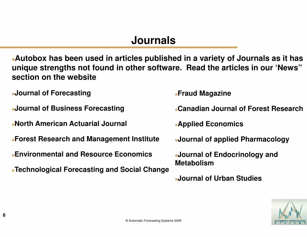
�Autobox has been used in articles published in a variety of Journals as it has unique strengths not found in other software. Read the articles in our ‘News” section on the website
�Journal of Forecasting
�Journal of Business Forecasting
�North American Actuarial Journal
�Forest Research and Management Institute
�Environmental and Resource Economics
�Technological Forecasting and Social Change
Journals
�Fraud Magazine
�Canadian Journal of Forest Research
�Applied Economics
�Journal of applied Pharmacology
�Journal of Endocrinology and Metabolism
�Journal of Urban Studies
Autobox Functionality
8
8© Automatic Forecasting Systems 2009
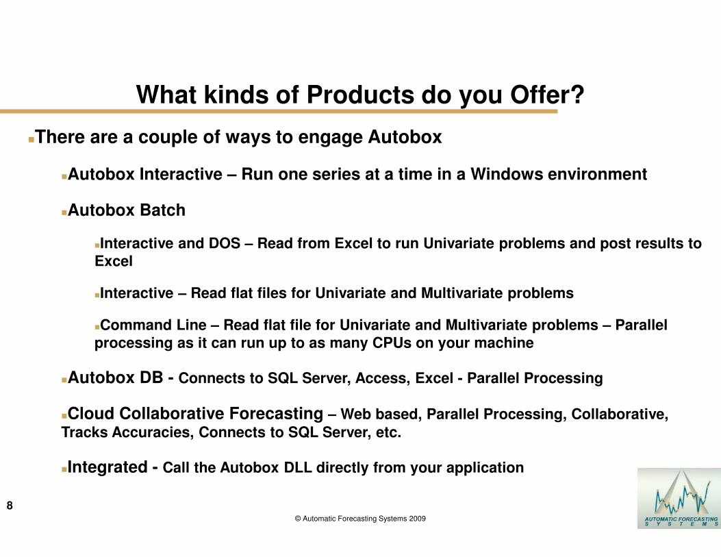
�There are a couple of ways to engage Autobox
�Autobox Interactive – Run one series at a time in a Windows environment
�Autobox Batch
�Interactive and DOS – Read from Excel to run Univariate problems and post results to
Excel
�Interactive – Read flat files for Univariate and Multivariate problems
�Command Line – Read flat file for Univariate and Multivariate problems – Parallel
processing as it can run up to as many CPUs on your machine
�Autobox DB - Connects to SQL Server, Access, Excel - Parallel Processing
�Cloud Collaborative Forecasting – Web based, Parallel Processing, Collaborative,
Tracks Accuracies, Connects to SQL Server, etc.
�Integrated - Call the Autobox DLL directly from your application
What kinds of Products do you Offer?
9
9© Automatic Forecasting Systems 2012
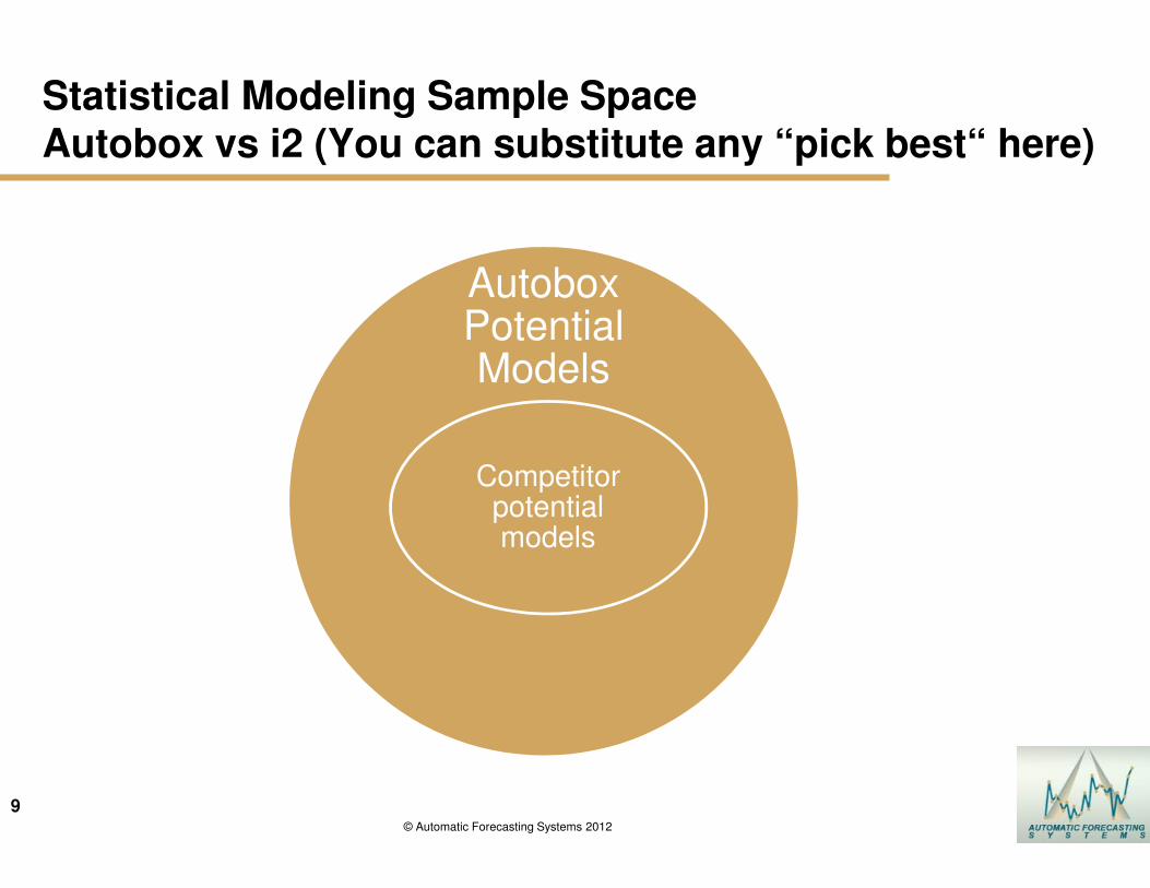
Statistical Modeling Sample Space Autobox vs i2 (You can substitute any “pick best“ here)
Autobox Potential Models
Competitor potential models
10
10© Automatic Forecasting Systems 2012
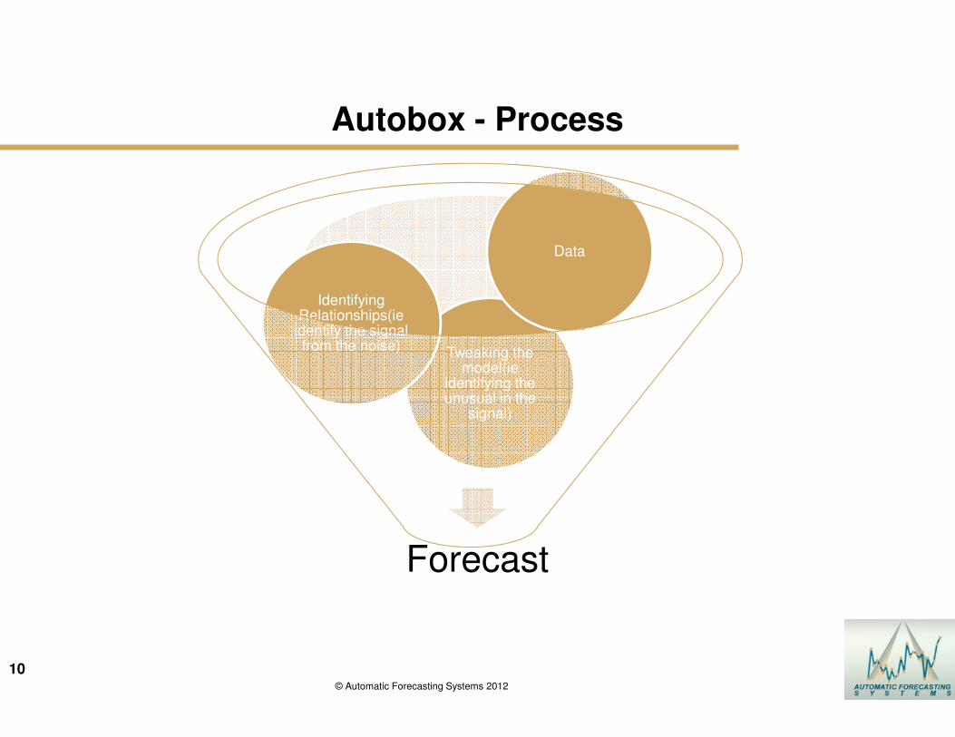
Autobox - Process
Forecast
Tweaking the model(ie
identifying the unusual in the
signal)
Identifying Relationships(ie
identify the signal from the noise)
Data
11
11© Automatic Forecasting Systems 2012
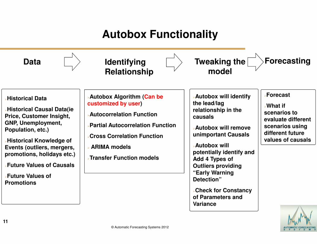
Autobox Functionality
�Autobox Algorithm (Can be customized by user)
�Autocorrelation Function
�Partial Autocorrelation Function
�Cross Correlation Function
� ARIMA models
�Transfer Function models
Identifying Relationship
ForecastingData
�Historical Data
�Historical Causal Data(ie Price, Customer Insight, GNP, Unemployment, Population, etc.)
�Historical Knowledge of Events (outliers, mergers, promotions, holidays etc.)
�Future Values of Causals
�Future Values of Promotions
�Autobox will identify the lead/lag relationship in the causals
�Autobox will remove unimportant Causals
�Autobox will potentially identify and Add 4 Types of
Outliers providing “Early Warning Detection”
�Check for Constancy of Parameters and Variance
Tweaking the model
�Forecast
�What if scenarios to evaluate different scenarios using different future values of causals
12
1212
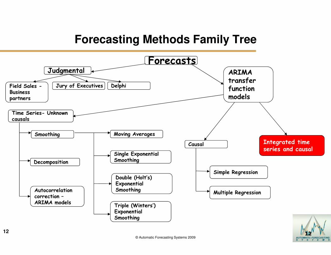
Forecasting Methods Family Tree
ForecastsJudgmental ARIMA
transfer function models
Causal
Time Series- Unknown causals
Integrated time series and causal
Autocorrelation correction –ARIMA models
Decomposition
Smoothing
DelphiJury of ExecutivesField Sales -Business partners
Moving Averages
Single Exponential Smoothing
Double (Holt’s) Exponential Smoothing
Triple (Winters’) Exponential Smoothing
Simple Regression
Multiple Regression
© Automatic Forecasting Systems 2009
13
13© Automatic Forecasting Systems 2009
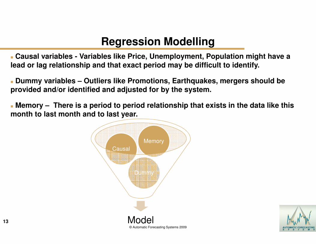
Regression Modelling
� Causal variables - Variables like Price, Unemployment, Population might have a
lead or lag relationship and that exact period may be difficult to identify.
� Dummy variables – Outliers like Promotions, Earthquakes, mergers should be provided and/or identified and adjusted for by the system.
� Memory – There is a period to period relationship that exists in the data like this
month to last month and to last year.
Model
Dummy
Causal
Memory
14© Automatic Forecasting Systems 2012
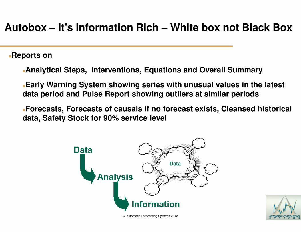
Autobox – It’s information Rich – White box not Black Box
�Reports on
�Analytical Steps, Interventions, Equations and Overall Summary
�Early Warning System showing series with unusual values in the latest data period and Pulse Report showing outliers at similar periods
�Forecasts, Forecasts of causals if no forecast exists, Cleansed historical data, Safety Stock for 90% service level
15
15© Automatic Forecasting Systems 2012
Specific ApplicationsWhat Can Autobox Be Used For?
�Data Cleansing - Correct historical data to what it should have been due to
misreporting or removing the impact of unexpected events(ie outliers)
�Causation – Does my advertising generate sales? Is Unemployment important?
Evaluate historical data to determine if a variable is important and what is the exact
time delay or lead?
�Forecasting – Forecast incorporating future expected events
�Short-Term and Long-Term Demand
�Daily Call Center Planning
�Intermittent Demand Data
�Financial - Probability of Hitting the Monthly # - Using Daily Data
�What-if Analysis – Forecast using different scenarios to assess expected impact by changing future causal values (ie 1% increase in unemployment)
�Early Warning System – Where are we underperforming/performing? Identify “most
unusual” SKU’s based on latest observation, trends, level
�Price Elasticities, but calculated with a robust model!© Automatic Forecasting Systems 2012
16
16© Automatic Forecasting Systems 2012
Why is Autobox’s Methodology Different?
�Automatically creates a customized model for every data set. Not “pick best”
�Automatically identifies and corrects outliers in the historical data and for the causal variables to keep the model used to forecast unaffected (Pulses, seasonal pulses, level shifts, local time trends)
�Automatically will identify and incorporate the time lead and lag relationship between the causal variables the variable being predicted
�Automatically will delete older data that behaves in a different “model” than the more recent data (i.e. Parameter Change detection via Chow Test)
�Automatically will weight observations based on their variance if there has been changes in historical volatility (i.e. Variance Change detection via Tsay Test)
�Automatically will identify intermittent demand data and use a special modelling approach to forecast the lumpy demand
17
17© Automatic Forecasting Systems 2009
How Autobox Treats Different Data Intervals You can (optionally) let the system do it all by itself!
�Incorporates variables for Hourly Data - Brings in Daily History and Forecast as a Causal Variable for the 24 separate regressions
�Incorporates variables for Daily data Automatically:
— Day of the week (i.e. Sundays are low)
— Special Days of the month (i.e. Social Security checks are delivered on the 3rd of the month)
— Week of the Year (i.e. 51 dummies Capturing seasonal variations) or Month of the Year (i.e. 11 dummies Capturing seasonal variations)
— Adds in holiday variables (including “Fridays before” holidays that fall on Mondays and Monday after a Friday Holiday AND a separate effect “long weekends”)
— End of the Month Effect – when last day of month is a Friday, Saturday or Sunday
�Incorporates variables for Weekly data:
— Trading Days (i.e. 19,19,22,20,21,21, etc.)
— Week of the Year (i.e. Capturing seasonal variations) Automatically
�Incorporates variables for Monthly data:
— Trading Days (i.e. 19,19,22,20,21,21, etc.)
— Month of the Year (i.e. 11 dummies Capturing seasonal variations)
— Accounting effect (i.e. 4/4/5)
– Accounting practice of uneven grouping of weeks into monthly buckets where there is a 4/4/5 pattern that is repeated
�Incorporates variables for Quarterly data:
— Quarterly effect (i.e. High in Q2)
Outliers will skew your model and forecast if not addressed
19
19© Automatic Forecasting Systems 2009
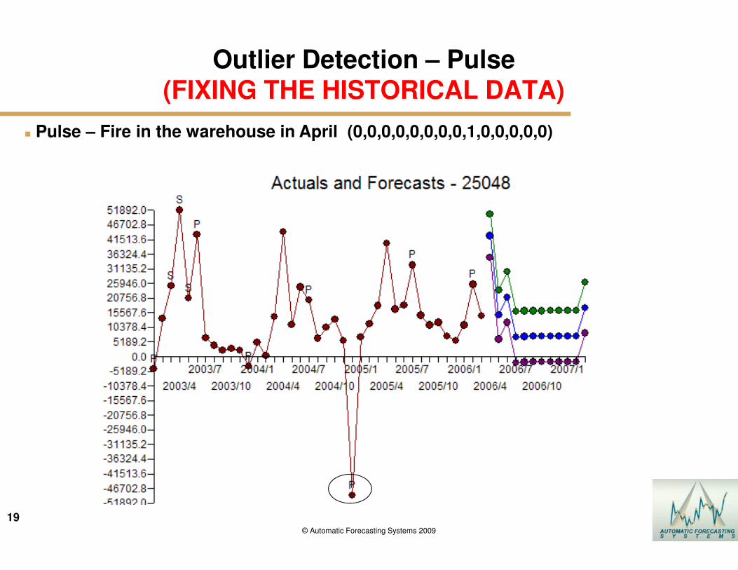
Outlier Detection – Pulse (FIXING THE HISTORICAL DATA)
� Pulse – Fire in the warehouse in April (0,0,0,0,0,0,0,0,1,0,0,0,0,0)
20
20© Automatic Forecasting Systems 2009
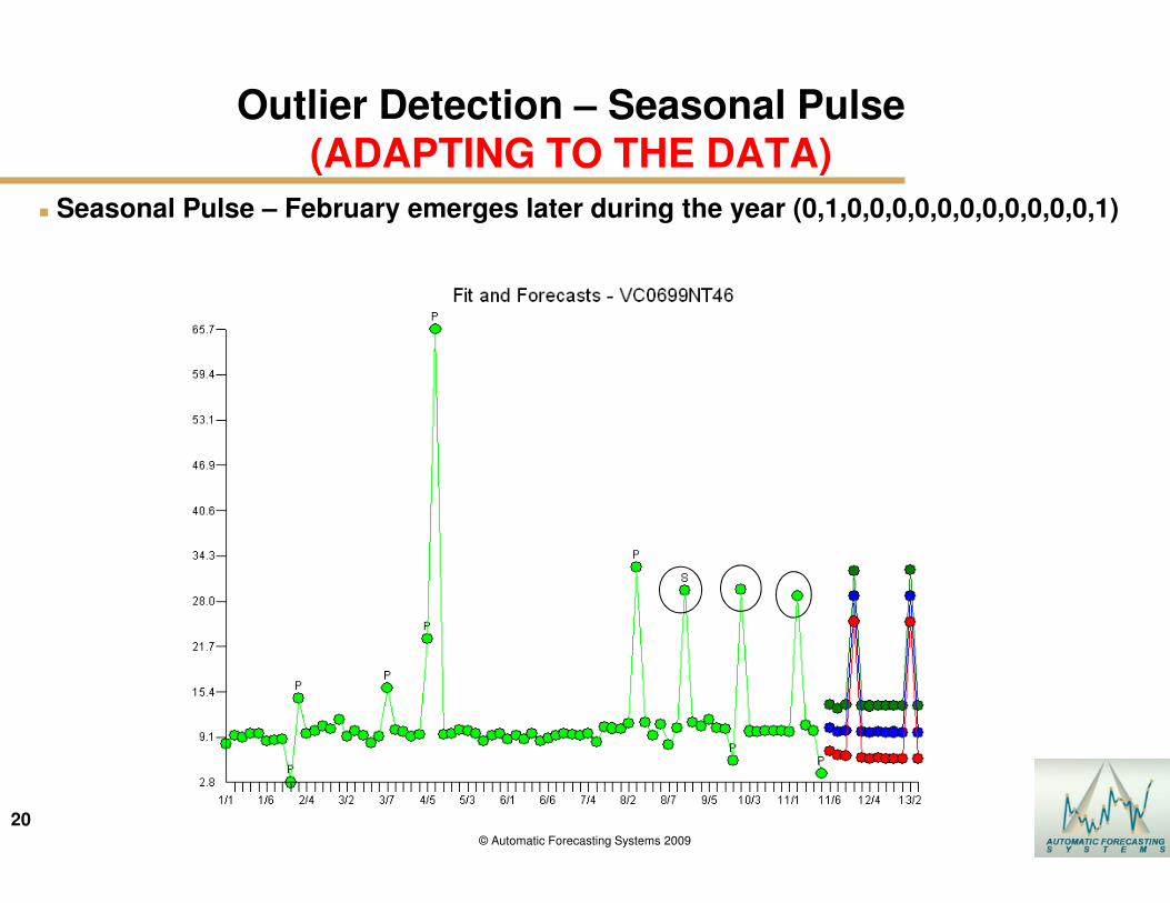
Outlier Detection – Seasonal Pulse (ADAPTING TO THE DATA)
� Seasonal Pulse – February emerges later during the year (0,1,0,0,0,0,0,0,0,0,0,0,0,1)
21
21© Automatic Forecasting Systems 2009
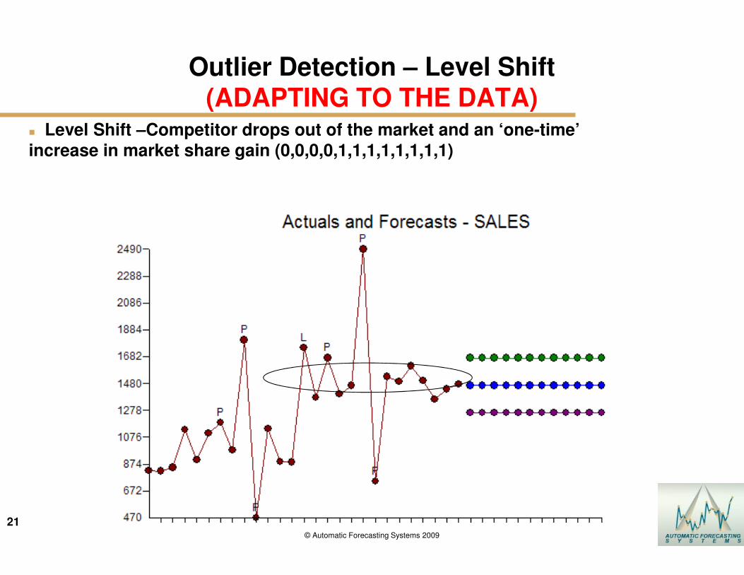
Outlier Detection – Level Shift(ADAPTING TO THE DATA)
� Level Shift –Competitor drops out of the market and an ‘one-time’
increase in market share gain (0,0,0,0,1,1,1,1,1,1,1,1)
22
22© Automatic Forecasting Systems 2009
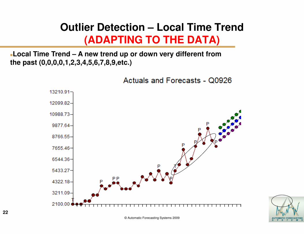
Outlier Detection – Local Time Trend(ADAPTING TO THE DATA)
�Local Time Trend – A new trend up or down very different from
the past (0,0,0,0,1,2,3,4,5,6,7,8,9,etc.)
23
23© Automatic Forecasting Systems 2009
What is unusual?
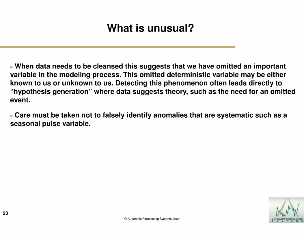
� When data needs to be cleansed this suggests that we have omitted an important
variable in the modeling process. This omitted deterministic variable may be either known to us or unknown to us. Detecting this phenomenon often leads directly to
“hypothesis generation” where data suggests theory, such as the need for an omitted
event.
� Care must be taken not to falsely identify anomalies that are systematic such as a seasonal pulse variable.
24
24© Automatic Forecasting Systems 2009
What is unusual?
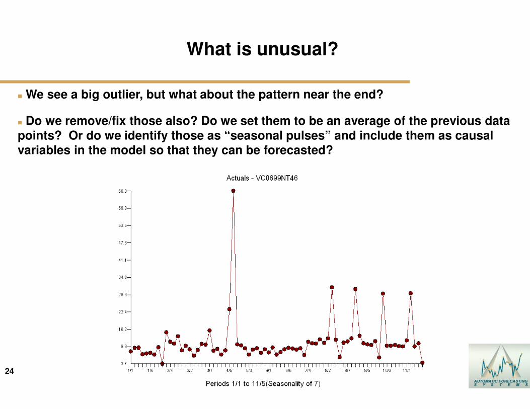
� We see a big outlier, but what about the pattern near the end?
� Do we remove/fix those also? Do we set them to be an average of the previous data
points? Or do we identify those as “seasonal pulses” and include them as causal variables in the model so that they can be forecasted?
25
25© Automatic Forecasting Systems 2009
What is unusual?
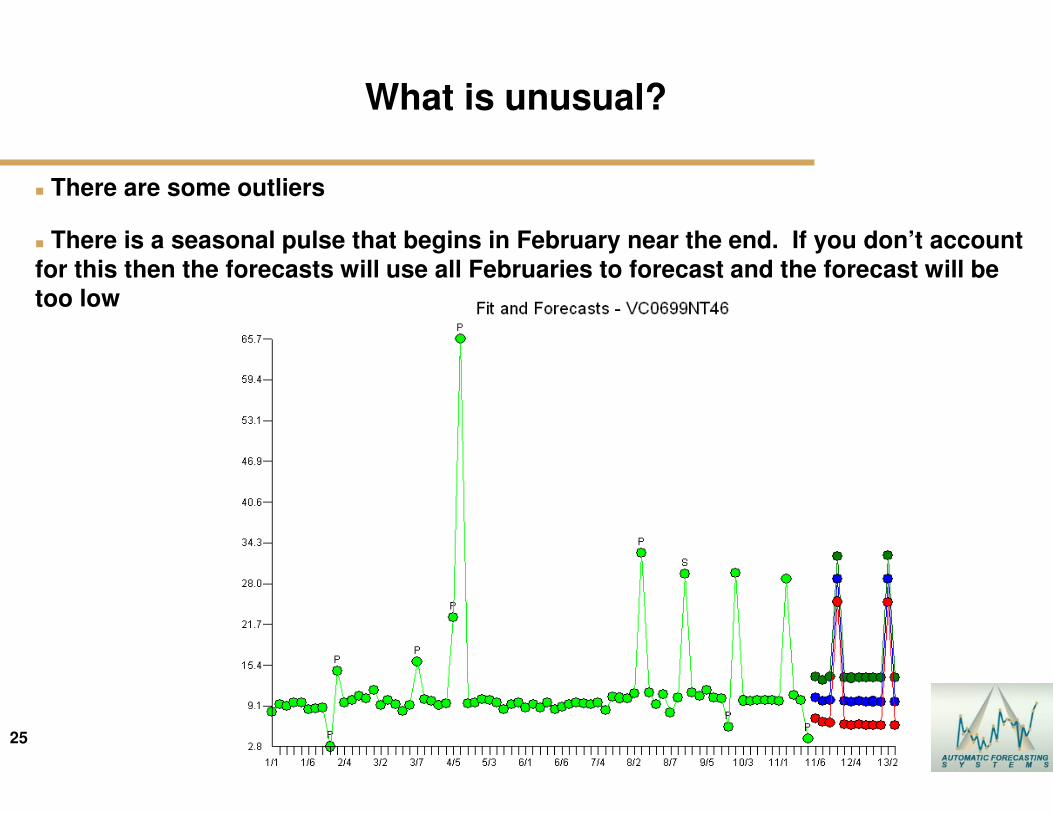
� There are some outliers
� There is a seasonal pulse that begins in February near the end. If you don’t account
for this then the forecasts will use all Februaries to forecast and the forecast will be too low
26
26© Automatic Forecasting Systems 2009
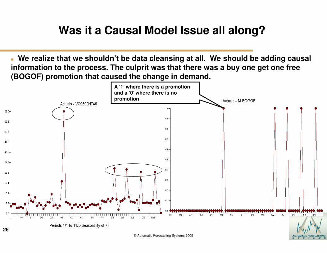
Was it a Causal Model Issue all along?
� We realize that we shouldn’t be data cleansing at all. We should be adding causal
information to the process. The culprit was that there was a buy one get one free (BOGOF) promotion that caused the change in demand.
A ‘1’ where there is a promotion and a ‘0’ where there is no promotion
27
27© Automatic Forecasting Systems 2009
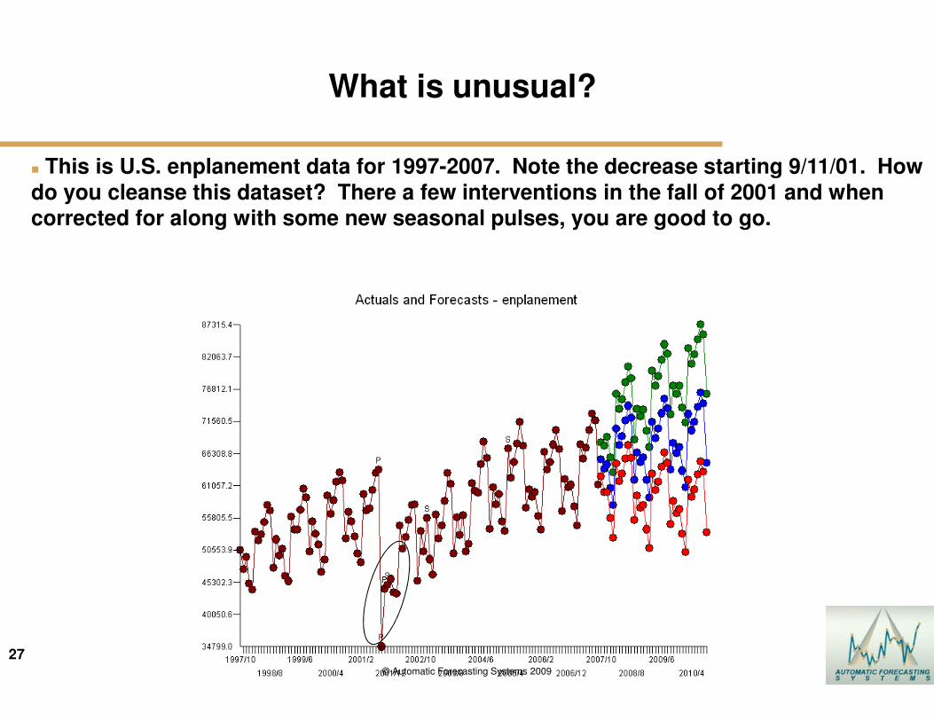
What is unusual?
� This is U.S. enplanement data for 1997-2007. Note the decrease starting 9/11/01. How
do you cleanse this dataset? There a few interventions in the fall of 2001 and when corrected for along with some new seasonal pulses, you are good to go.
28
28© Automatic Forecasting Systems 2009
What is unusual?
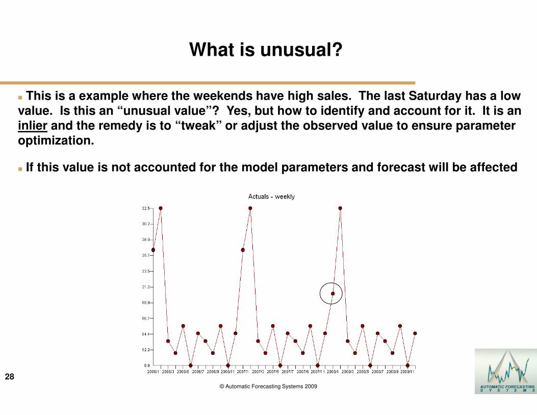
� This is a example where the weekends have high sales. The last Saturday has a low
value. Is this an “unusual value”? Yes, but how to identify and account for it. It is an inlier and the remedy is to “tweak” or adjust the observed value to ensure parameter
optimization.
� If this value is not accounted for the model parameters and forecast will be affected
29
29© Automatic Forecasting Systems 2009
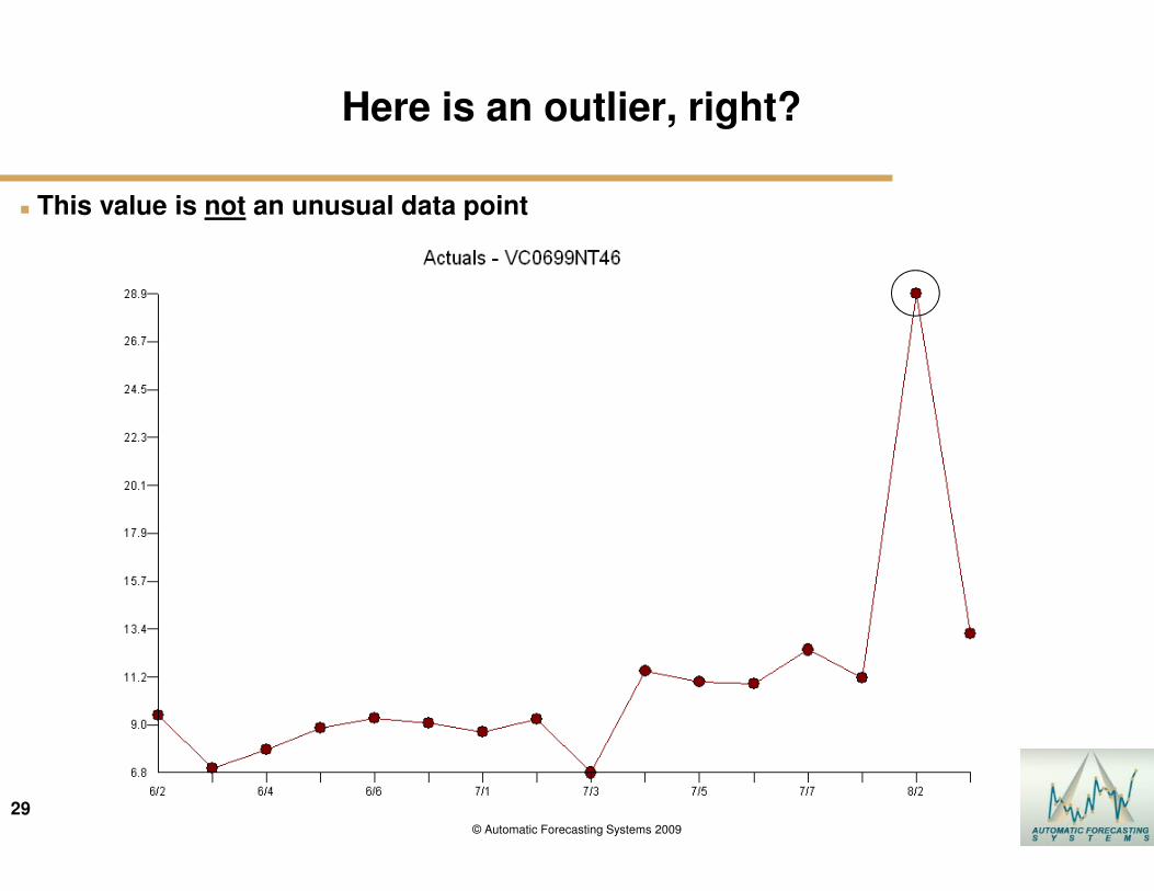
Here is an outlier, right?
� This value is not an unusual data point
30
30© Automatic Forecasting Systems 2009
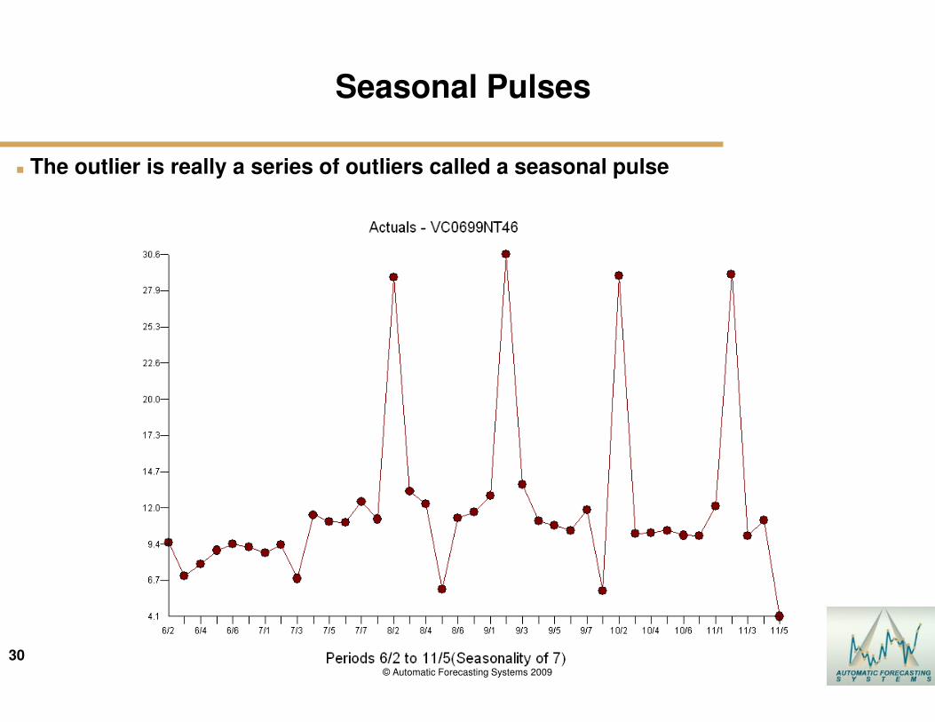
Seasonal Pulses
� The outlier is really a series of outliers called a seasonal pulse
31
31© Automatic Forecasting Systems 2012
Autobox and Inliers
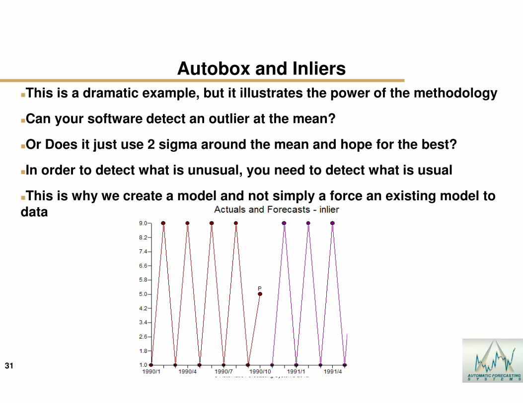
�This is a dramatic example, but it illustrates the power of the methodology
�Can your software detect an outlier at the mean?
�Or Does it just use 2 sigma around the mean and hope for the best?
�In order to detect what is unusual, you need to detect what is usual
�This is why we create a model and not simply a force an existing model to data
32
32© Automatic Forecasting Systems 2009
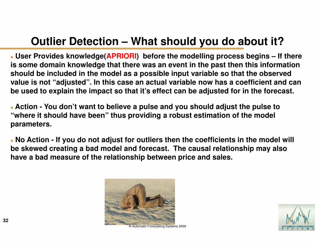
Outlier Detection – What should you do about it?
� User Provides knowledge(APRIORI) before the modelling process begins – If there
is some domain knowledge that there was an event in the past then this information should be included in the model as a possible input variable so that the observed
value is not “adjusted”. In this case an actual variable now has a coefficient and can
be used to explain the impact so that it’s effect can be adjusted for in the forecast.
� Action - You don’t want to believe a pulse and you should adjust the pulse to “where it should have been” thus providing a robust estimation of the model
parameters.
� No Action - If you do not adjust for outliers then the coefficients in the model will
be skewed creating a bad model and forecast. The causal relationship may also have a bad measure of the relationship between price and sales.
33
33© Automatic Forecasting Systems 2012
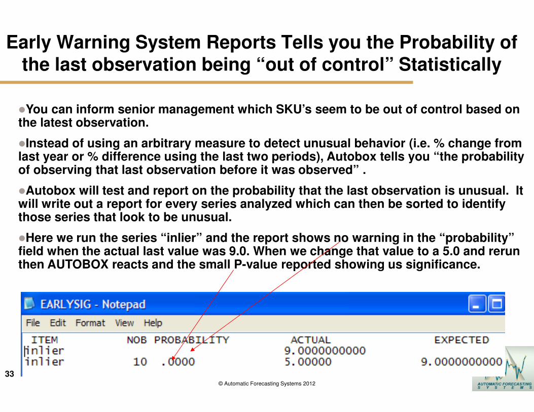
Early Warning System Reports Tells you the Probability of the last observation being “out of control” Statistically
�You can inform senior management which SKU’s seem to be out of control based on the latest observation.
�Instead of using an arbitrary measure to detect unusual behavior (i.e. % change from last year or % difference using the last two periods), Autobox tells you “the probability of observing that last observation before it was observed” .
�Autobox will test and report on the probability that the last observation is unusual. It will write out a report for every series analyzed which can then be sorted to identify those series that look to be unusual.
�Here we run the series “inlier” and the report shows no warning in the “probability” field when the actual last value was 9.0. When we change that value to a 5.0 and rerun then AUTOBOX reacts and the small P-value reported showing us significance.
34
34© Automatic Forecasting Systems 2008
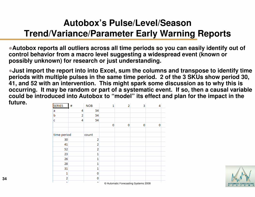
Autobox’s Pulse/Level/Season Trend/Variance/Parameter Early Warning Reports
�Autobox reports all outliers across all time periods so you can easily identify out of control behavior from a macro level suggesting a widespread event (known or possibly unknown) for research or just understanding.
�Just import the report into into Excel, sum the columns and transpose to identify time periods with multiple pulses in the same time period. 2 of the 3 SKUs show period 30, 41, and 52 with an intervention. This might spark some discussion as to why this is occurring. It may be random or part of a systematic event. If so, then a causal variable could be introduced into Autobox to “model” its effect and plan for the impact in the future.
35
35© Automatic Forecasting Systems 2012
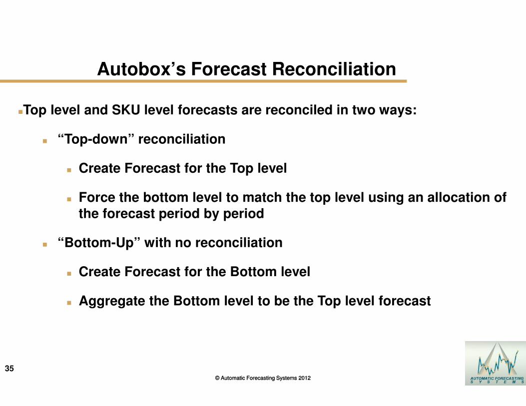
Autobox’s Forecast Reconciliation
�Top level and SKU level forecasts are reconciled in two ways:
� “Top-down” reconciliation
� Create Forecast for the Top level
� Force the bottom level to match the top level using an allocation of the forecast period by period
� “Bottom-Up” with no reconciliation
� Create Forecast for the Bottom level
� Aggregate the Bottom level to be the Top level forecast
© Automatic Forecasting Systems 2012

Using Causal Variables

37
37© Automatic Forecasting Systems 2009
Two Types of Users Rear View Mirror vs. Rear and Front Windshield
�Use the History of the data only
�Use the History of the data AND causal variables (i.e. holidays, price, marketing promotions, advertising) and the future values of these variables.
+
38
Case Study – What-if Analysis
© Automatic Forecasting Systems 2011
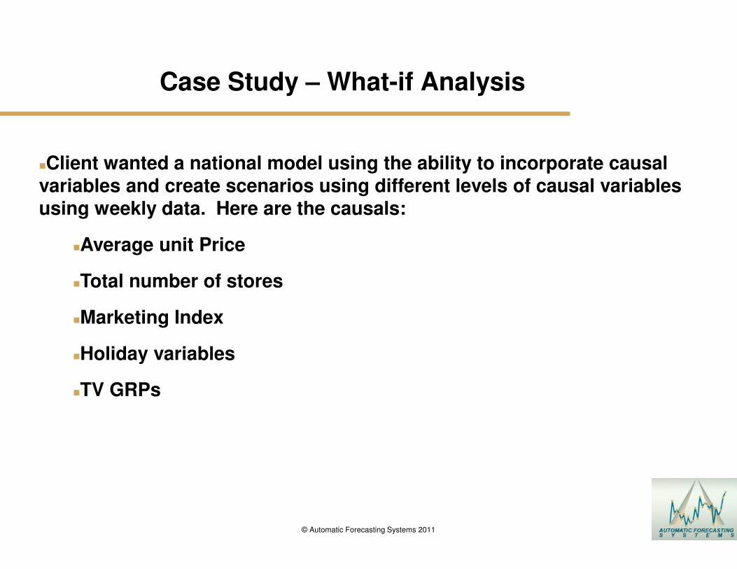
�Client wanted a national model using the ability to incorporate causal variables and create scenarios using different levels of causal variables using weekly data. Here are the causals:
�Average unit Price
�Total number of stores
�Marketing Index
�Holiday variables
�TV GRPs

39
39© Automatic Forecasting Systems 2012
Case Study – What-if Analysis Baseline Forecast
© Automatic Forecasting Systems 2012
40
40© Automatic Forecasting Systems 2012
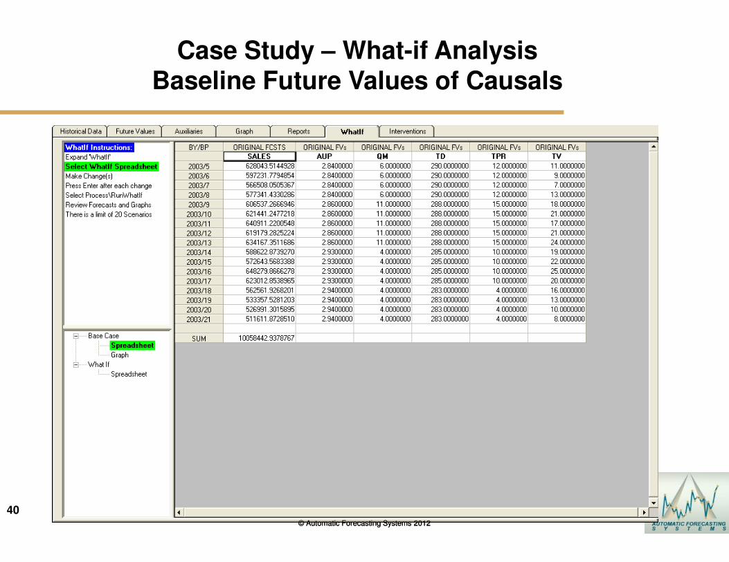
Case Study – What-if Analysis Baseline Future Values of Causals
© Automatic Forecasting Systems 2012

41
41
Case Study – What-if Analysis Scenario #1 Adjust Price and TV Spots Up
© Automatic Forecasting Systems 2012© Automatic Forecasting Systems 2012
42
42© Automatic Forecasting Systems 2012
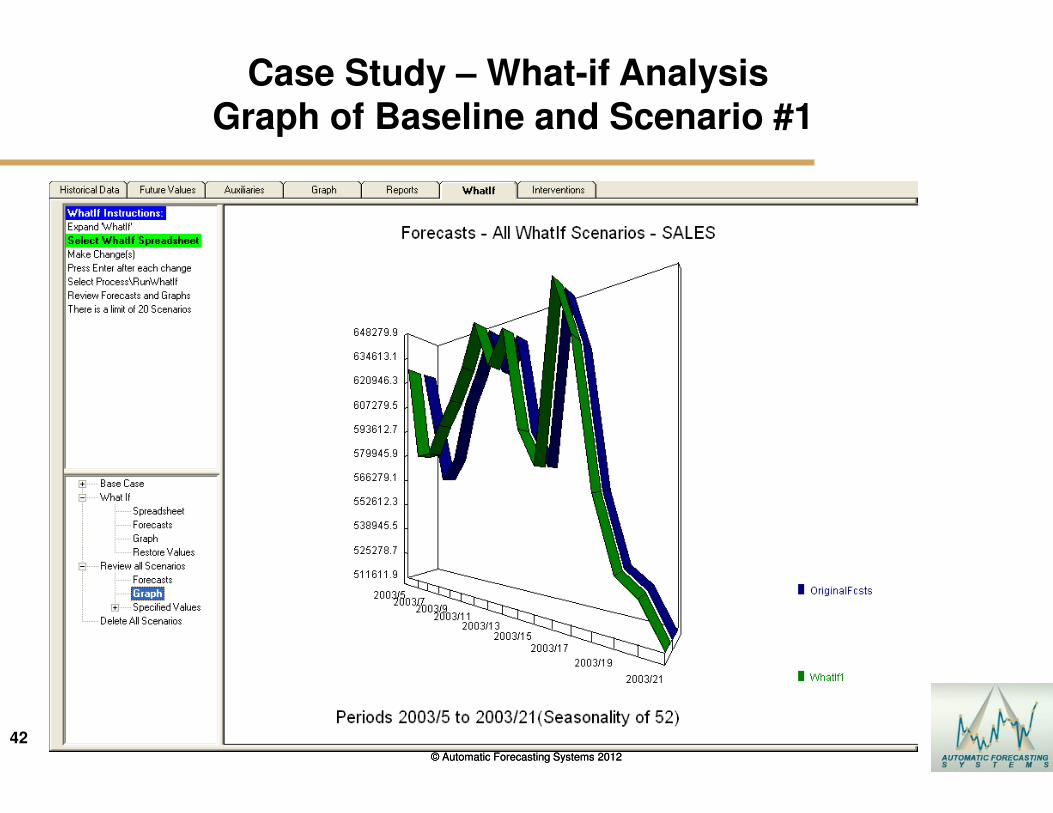
Case Study – What-if AnalysisGraph of Baseline and Scenario #1
© Automatic Forecasting Systems 2012
Three Examples
44
44© Automatic Forecasting Systems 2012
Financial Forecasting ExampleHow is your Finance Team doing this now?
� The 2008 financial crises caught a few companies unable to quickly identify when month end numbers were not going to be met.
�Simplistic approaches use a ratio estimate (ie 5 days into the month 30/5 so multiply current month total by 6 to get month end estimate) are simplistic and incorrect. Promotions and day of the week effects are not considered using ratio estimates and need to be modeled at a DAILY level as part of a comprehensive model and forecast which can then be used to determine probabilities of making the month end number.
� Autobox reports out a variety of Probabilities which the target can be evaluated against. A summary report can then be used to identify which SKU’s are likely NOT to make the month end number.
What's the probability of making the month end targeted number given the most recent daily observation?
45
45© Automatic Forecasting Systems 2012
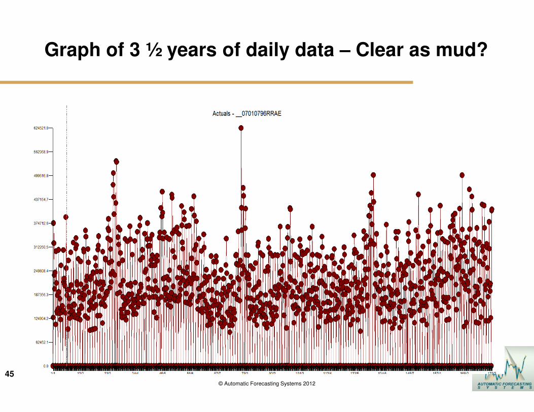
Graph of 3 ½ years of daily data – Clear as mud?
46
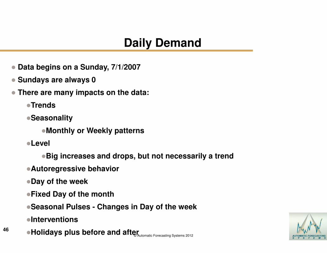
46© Automatic Forecasting Systems 2012
Daily Demand
� Data begins on a Sunday, 7/1/2007
� Sundays are always 0
� There are many impacts on the data:
�Trends
�Seasonality
�Monthly or Weekly patterns
�Level
�Big increases and drops, but not necessarily a trend
�Autoregressive behavior
�Day of the week
�Fixed Day of the month
�Seasonal Pulses - Changes in Day of the week
�Interventions
�Holidays plus before and after
47
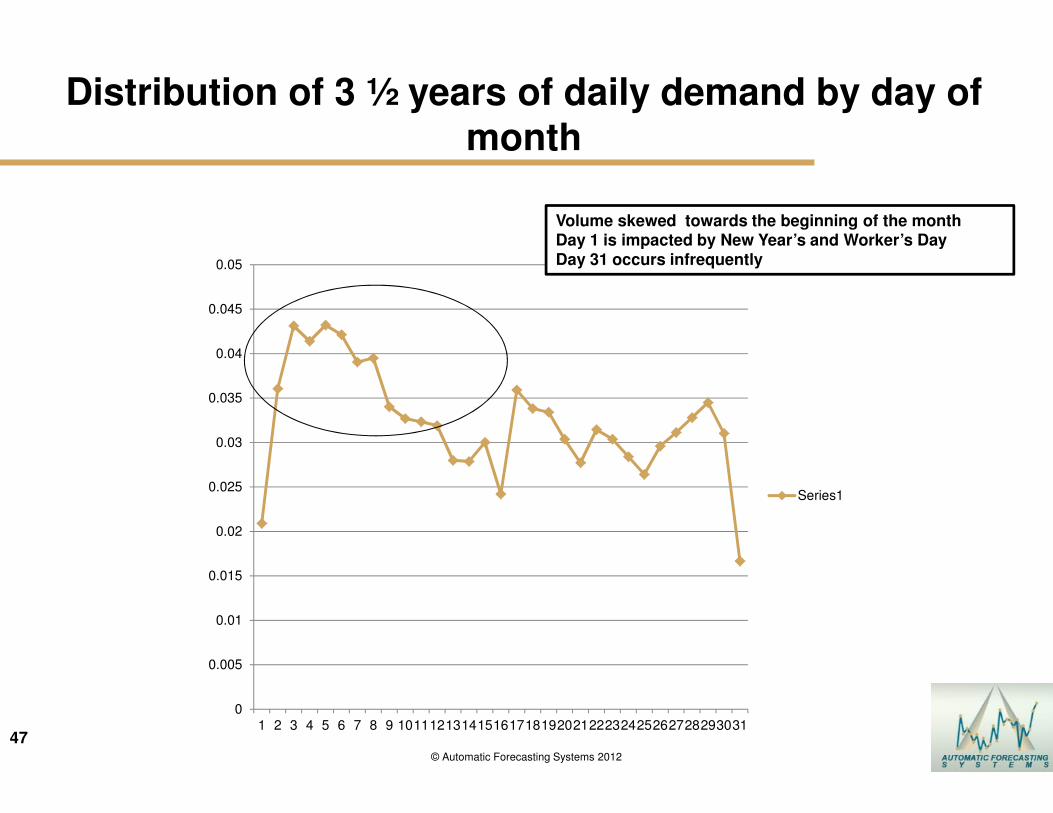
47© Automatic Forecasting Systems 2012
Distribution of 3 ½ years of daily demand by day of month
0
0.005
0.01
0.015
0.02
0.025
0.03
0.035
0.04
0.045
0.05
1 2 3 4 5 6 7 8 9 10111213141516171819202122232425262728293031
Series1
Volume skewed towards the beginning of the month Day 1 is impacted by New Year’s and Worker’s DayDay 31 occurs infrequently
48
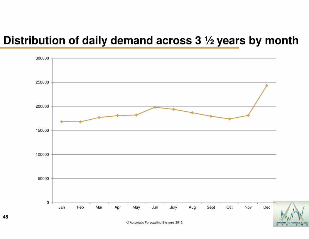
48© Automatic Forecasting Systems 2012
Distribution of daily demand across 3 ½ years by month
0
50000
100000
150000
200000
250000
300000
Jan Feb Mar Apr May Jun July Aug Sept Oct Nov Dec
49
49© Automatic Forecasting Systems 2012
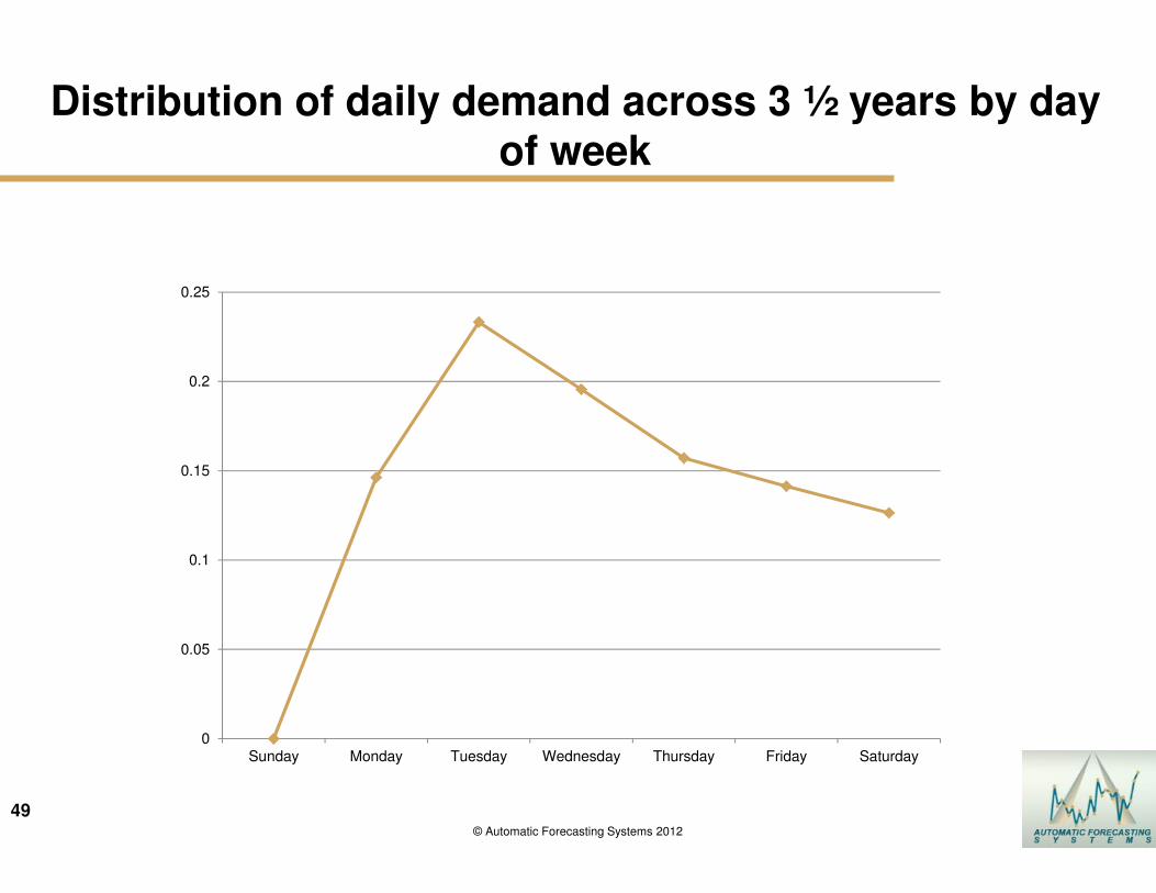
Distribution of daily demand across 3 ½ years by day of week
0
0.05
0.1
0.15
0.2
0.25
Sunday Monday Tuesday Wednesday Thursday Friday Saturday
50
50© Automatic Forecasting Systems 2012
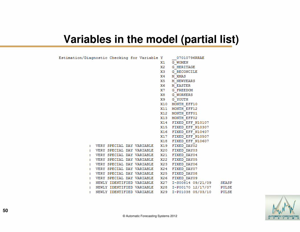
Variables in the model (partial list)
51
51© Automatic Forecasting Systems 2012
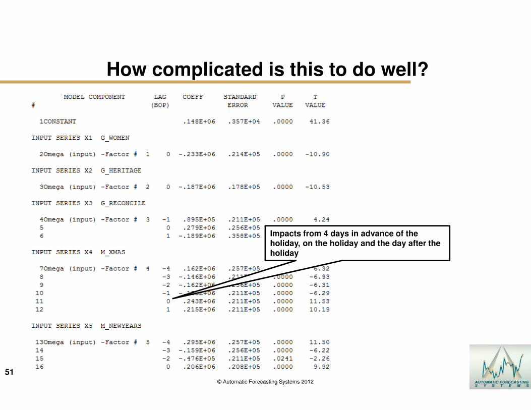
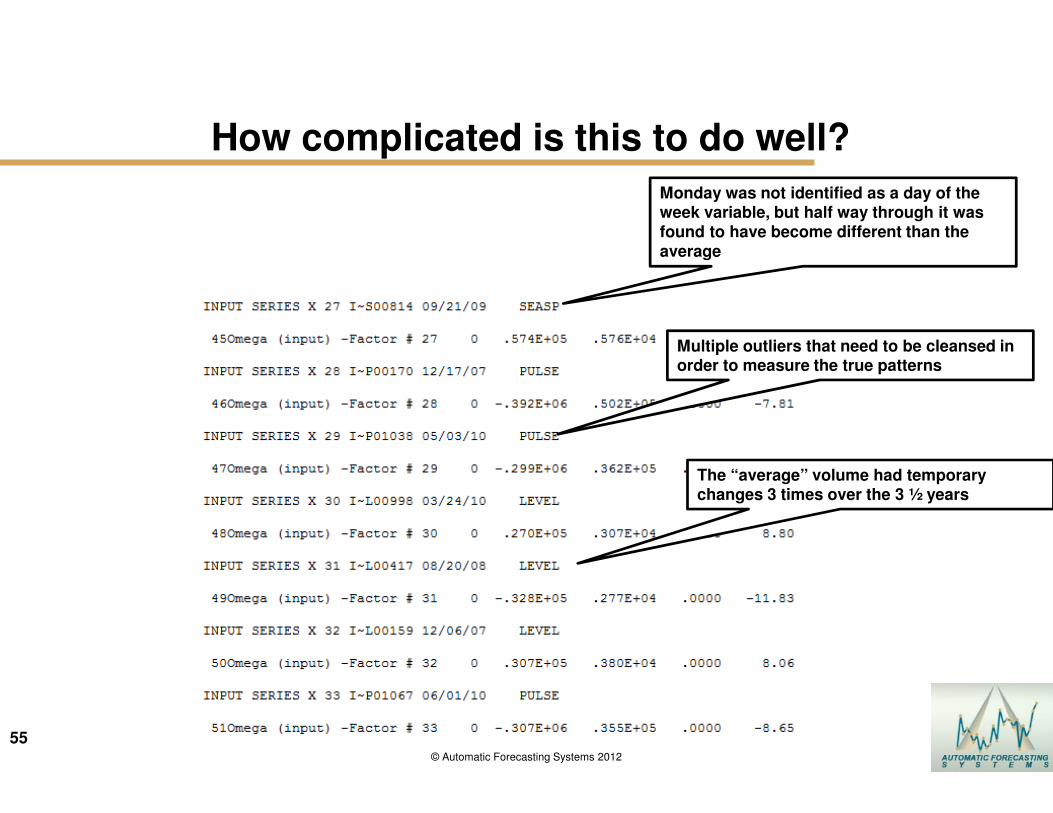
How complicated is this to do well?
Impacts from 4 days in advance of the holiday, on the holiday and the day after the holiday
52
52© Automatic Forecasting Systems 2012
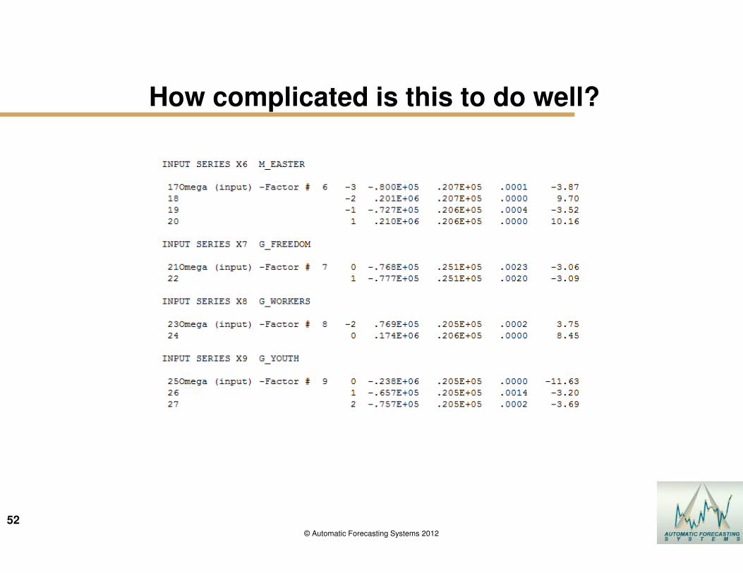
How complicated is this to do well?
53
53© Automatic Forecasting Systems 2012
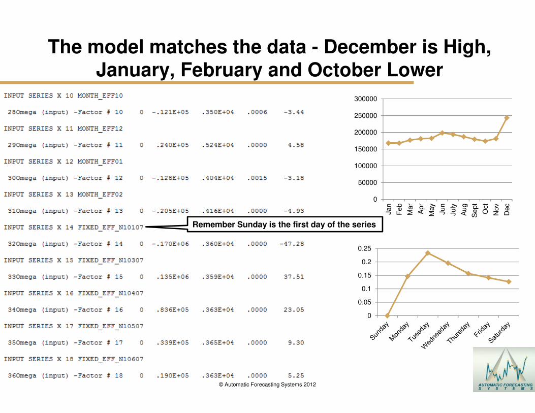
The model matches the data - December is High, January, February and October Lower
0
50000
100000
150000
200000
250000
300000
Jan
Feb
Mar
Ap
r
May
Jun
July
Au
g
Se
pt
Oct
Nov
Dec
0
0.05
0.1
0.15
0.2
0.25
Remember Sunday is the first day of the series
54
54© Automatic Forecasting Systems 2012
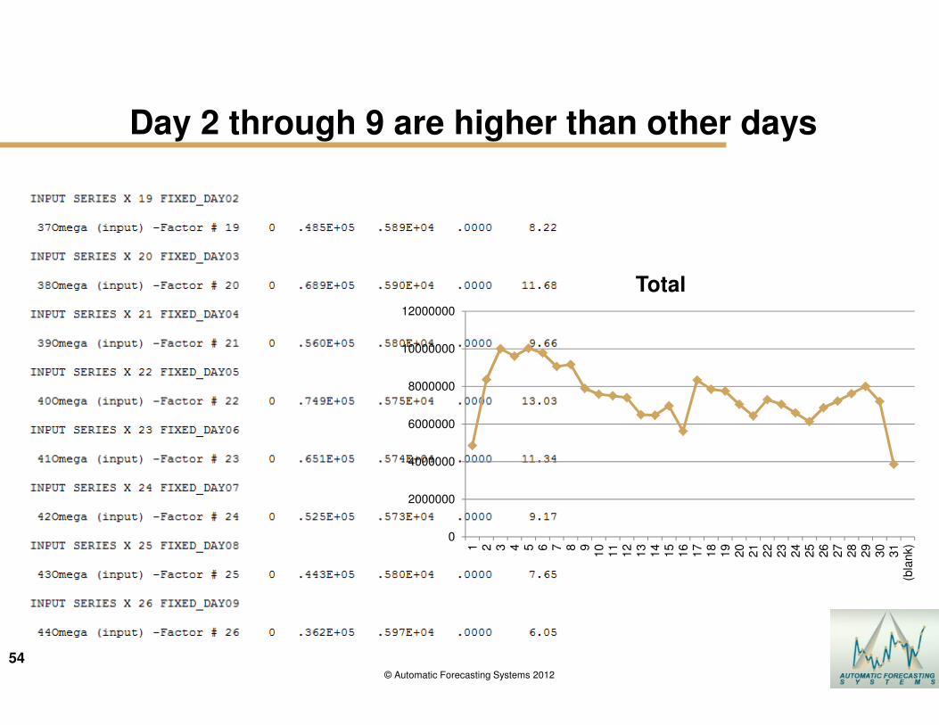
Day 2 through 9 are higher than other days
0
2000000
4000000
6000000
8000000
10000000
12000000
1 2 3 4 5 6 7 8 910
11
12
13
14
15
16
17
18
19
20
21
22
23
24
25
26
27
28
29
30
31
(bla
nk)
Total
55
55© Automatic Forecasting Systems 2012
How complicated is this to do well?
Monday was not identified as a day of the week variable, but half way through it was found to have become different than the average
Multiple outliers that need to be cleansed in order to measure the true patterns
The “average” volume had temporary changes 3 times over the 3 ½ years
56
56© Automatic Forecasting Systems 2012
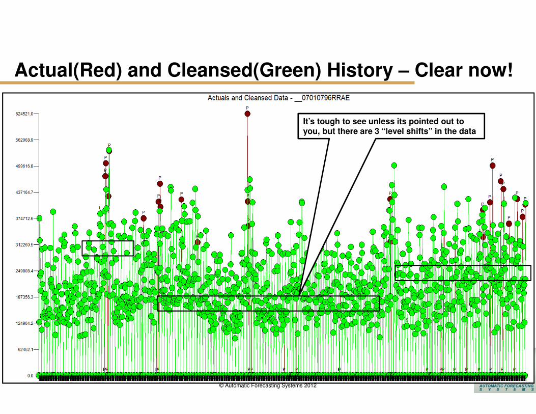
Actual(Red) and Cleansed(Green) History – Clear now!
It’s tough to see unless its pointed out to you, but there are 3 “level shifts” in the data
57
57© Automatic Forecasting Systems 2009
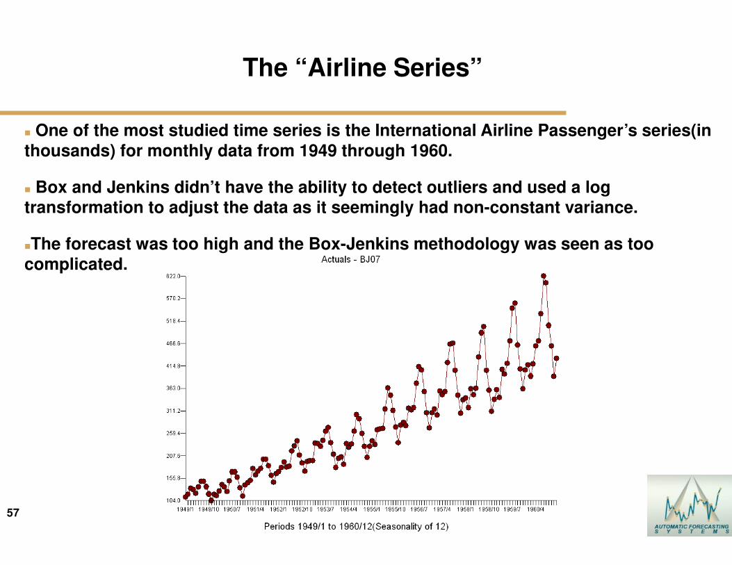
The “Airline Series”
� One of the most studied time series is the International Airline Passenger’s series(in
thousands) for monthly data from 1949 through 1960.
� Box and Jenkins didn’t have the ability to detect outliers and used a log transformation to adjust the data as it seemingly had non-constant variance.
�The forecast was too high and the Box-Jenkins methodology was seen as too
complicated.
58
58© Automatic Forecasting Systems 2009
The “Airline Series”
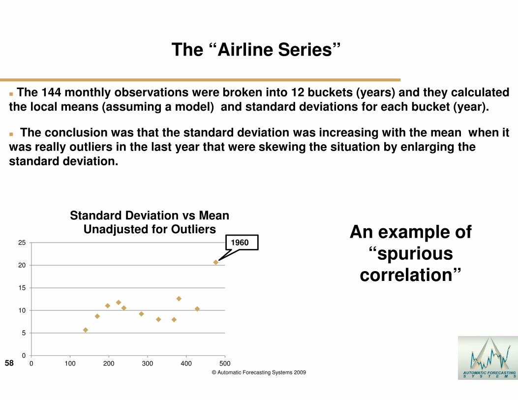
� The 144 monthly observations were broken into 12 buckets (years) and they calculated
the local means (assuming a model) and standard deviations for each bucket (year).
� The conclusion was that the standard deviation was increasing with the mean when it was really outliers in the last year that were skewing the situation by enlarging the
standard deviation.
0
5
10
15
20
25
0 100 200 300 400 500
Standard Deviation vs Mean Unadjusted for Outliers
1960An example of
“spurious correlation”
59
59© Automatic Forecasting Systems 2009
The “Airline Series”
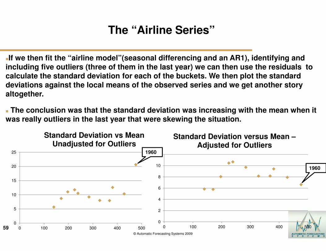
�If we then fit the “airline model”(seasonal differencing and an AR1), identifying and
including five outliers (three of them in the last year) we can then use the residuals to calculate the standard deviation for each of the buckets. We then plot the standard
deviations against the local means of the observed series and we get another story
altogether.
� The conclusion was that the standard deviation was increasing with the mean when it was really outliers in the last year that were skewing the situation.
0
2
4
6
8
10
12
0 100 200 300 400 500
Standard Deviation versus Mean –Adjusted for Outliers
1960
1960
0
5
10
15
20
25
0 100 200 300 400 500
Standard Deviation vs Mean Unadjusted for Outliers
60
60© Automatic Forecasting Systems 2009
Did you spot the outliers in 1960?
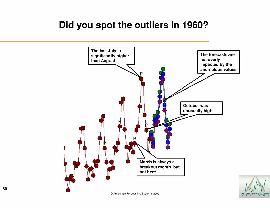
The last July is significantly higher than August
October was unusually high
March is always a breakout month, but not here
The forecasts are not overly impacted by the anomolous values
61
61© Automatic Forecasting Systems 2012
SAP APO in the International Journal of Applied Forecasting Foresight Issue Fall 2006 – p 52
The Standard Forecasting Tools in APO
�Moving Averages and weighted moving averages
�A portion of the family of exponential smoothing methods (a notable exclusion being the set of procedures that assume multiplicative seasonality)
�Automatic model selection in which the system chooses among included members of the exponential smoothing family
�Croston’s model for intermittent demand (without the Syntetos and Boylan(2005) corrections)
�Simple and multiple regressions
© Automatic Forecasting Systems 2012
62
62© Automatic Forecasting Systems 2012
SAP APO in the International Journal of Applied Forecasting Foresight Issue Fall 2006 – p 54
Summary
SAP APO is focusing on the whole supply chain and also on planning and process consistency. The mathematical accuracy of its forecasts may be worse than that of a stand-alone forecasting package, but the benefits to our company in terms of worldwide network planning and control more than compensate for this.
© Automatic Forecasting Systems 2012
63
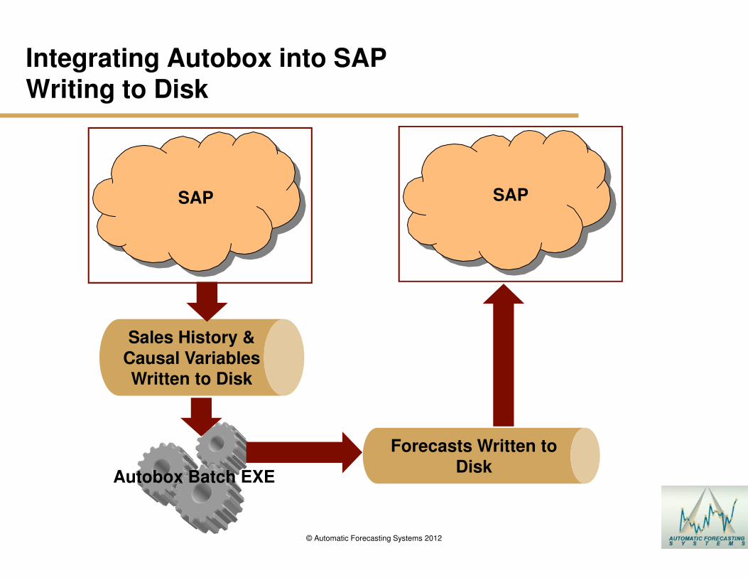
Integrating Autobox into SAPWriting to Disk
Sales History &
Causal Variables Written to Disk
SAP
Autobox Batch EXE
Forecasts Written to
Disk
SAP
© Automatic Forecasting Systems 2012

64
Integrating Autobox into SAPCalling a DLL and What-if Scenario
SAP
Autobox DLL
SAP
Forecasts Written or Passed
to an application to do What-if Scenarios.
Forecasts Passed to
Autobox in memory.
© Automatic Forecasting Systems 2012

65
65© Automatic Forecasting Systems 2012
Linkedin.com
Make sure to join the Autobox discussion group on linkedin.com