Can You Spot the Fakes? On the Limitations ofUser Feedback in Online Social Networks

David Mandell FreemanLinkedIn Corporation, USA

dfreeman@linkedin.com

ABSTRACTOnline social networks (OSNs) are appealing platforms forspammers and fraudsters, who typically use fake or compro-mised accounts to connect with and defraud real users. Tocombat such abuse, OSNs allow users to report fraudulentprofiles or activity. The OSN can then use reporting datato review and/or limit activity of reported accounts.

Previous authors have suggested that an OSN can aug-ment its takedown algorithms by identifying a “trusted set”of users whose reports are weighted more heavily in the dis-position of flagged accounts. Such identification would allowthe OSN to improve both speed and accuracy of fake accountdetection and thus reduce the impact of spam on users.

In this work we provide the first public, data-driven as-sessment of whether the above assumption is true: are someusers better at reporting than others? Specifically, is re-porting skill both measurable, i.e., possible to distinguishfrom random guessing; and repeatable, i.e., persistent overrepeated sampling?

Our main contributions are to develop a statistical frame-work that describes these properties and to apply this frame-work to data from LinkedIn, the professional social network.Our data includes member reports of fake profiles as wellas the more voluminous, albeit weaker, signal of memberresponses to connection requests. We find that membersdemonstrating measurable, repeatable skill in identifyingfake profiles do exist but are rare: at most 2.4% of thosereporting fakes and at most 1.3% of those rejecting connec-tion requests. We conclude that any reliable “trusted set”of members will be too small to have noticeable impact onspam metrics.

Keywords: Social networks; spam detection; online trust;fake accounts; reputation systems.

1. INTRODUCTIONOnline social networks’ ubiquity and popularity make them

appealing platforms for spammers and fraudsters to exe-cute their dirty deeds. Since most large OSNs (e.g. Face-

c©2017 International World Wide Web Conference Committee(IW3C2), published under Creative Commons CC BY 4.0 License.WWW 2017, April 3–7, 2017, Perth, Australia.ACM 978-1-4503-4913-0/17/04.http://dx.doi.org/10.1145/3038912.3052706

.

book [11, §4] and LinkedIn [16, §8]) require user accountsto reflect a real identity, malicious actors use fake or com-promised accounts to connect with and defraud real, unsus-pecting users of the platform. Combatting fake accounts(also known as sybils) and preventing unauthorized accesshave thus received much attention from both researchers andpractitioners, and there is a large body of work on fake ac-count detection [5,6,9,19,24,26,28,29] and account takeoverprevention [2–4,13] in the literature.

To help combat this abuse, OSNs make available to usersa variety of mechanisms for reporting fraudulent profiles oractivity, such as“flag”or“report spam” interfaces. The OSNcan then review and/or limit activity of accounts that havebeen reported, for example if a user receives too many re-ports in a given time period. In addition, there may bemechanisms for users to take positive action on real accounts(e.g., accept an invitation request), which can also serve asa form of reporting.

It seems reasonable to assume that some users are moreadept at distinguishing fake profiles from real ones; indeed,several previous works on identifying spam or fake accountshave made use of this assumption [6, 7, 25, 30]. If this as-sumption is true, then the OSN can augment its takedownalgorithms by identifying a “trusted set” of users whose feed-back is weighted more heavily in the disposition of flaggedaccounts. Such identification would allow the OSN to im-prove both speed and accuracy of fake account detection andthus reduce the impact of spam on users.1

While the potential for leveraging high-quality reportersseems high, to date there has been no rigorous publishedstudy of reporting ability in real-life social networks. Thegoal of this paper is thus to test the following hypothesis:There are some social network users who are good at iden-tifying fake accounts.

1.1 Our contributionIn this work we provide the first public, data-driven as-

sessment of user feedback signals in the context of reportingfake accounts in online social networks. In particular:

• We provide a statistical framework for assessing userreporting skill. If flagging is a real skill, it must be mea-surable; that is, we should be able to determine whichusers are particularly skilled at flagging and quantifyhow skilled they are. Furthermore, flagging skill must

1To prevent manipulation of the flagging signal, any“trusted” label should not be exposed to the end user (ei-ther directly or indirectly).

be repeatable; that is, a user who demonstrates supe-rior flagging ability in one data set should be able todemonstrate the same ability on a different sample orat a different point in time. If flagging is measurablebut not repeatable then even once we identify goodflaggers, the OSN cannot use their future flagging ac-tivity to help catch fake accounts.

• We apply our framework to data from LinkedIn, theprofessional social network. We consider three differ-ent signals: flagging of fake profiles, accepting connec-tion requests, and rejecting connection requests. Wefind that members demonstrating measurable, repeat-able skill in identifying fake profiles exist but are rare:at most 2.4% of members reporting fake accounts overa six-month period, and at most 1.3% of members re-jecting connection requests over a one-month period.We also find that up to 3.8% of members acceptingconnection requests show skill in identifying real ac-counts.

We note that our analysis is concerned with aggregatingreporting signals by reporter. LinkedIn and many othersocial networks also aggregate signals by reportee; indeed,a primary motivation for this work is to explore whetherreporter-based signals might be effectively incorporated intoexisting reportee-based systems.

We note further that all signals in our data set were col-lected organically, without specifically instructing users tolook out for fake accounts. This leaves open the question ofwhether targeted user prompting or some other offical spam-finding program would increase the prevalence of skilled re-porters.

1.2 Related workZheleva et al. [30] describe a system for email spam fil-

tering that uses the very kind of reporter reputation whoseexistence we are trying to establish, and Chen et al. [7] de-velop a similar system for fighting SMS spam. Both pa-pers propose a framework in which reports of reliable usersare weighted more highly in classifying spam, and providea mechanism for evolving reporter reputation over time asnew reports come in. However, the system of Zheleva et al.requires “an initial set of users who have proven to be re-liable in the past,” and the authors implicitly assume thatsuch a set both (a) can be identified and (b) will continue tobe reliable in the future. Our work calls into question thisassumption, at least in the domain of social networks.

Wang et al. [25] describe a crowdsourcing study in whichworkers are shown accounts and asked to label them as realor fake. They find that in this artificial setting, “peoplecan identify differences between Sybil and legitimate pro-files, but most individual testers are not accurate enoughto be reliable.” They quantify this reliability only in termsof accuracy and do not attempt to test repeatability of theworkers’ labeling.

Moore and Clayton [20] and Chia and Knapskog [8] havestudied the “wisdom of crowds” in reporting phishing andweb vulnerabilities, respectively. Both studies find a power-law distribution in participation rates, and the former findsthat more frequent reporters achieve higher accuracy andrecommend that “the views of inexperienced users shouldperhaps be assigned less weight when compared to highlyexperienced users.” However, Moore and Clayton do not

suggest how such a weight should be determined algorith-mically, nor do they consider repeatability.

Cao et al. [6] use negative feedback such as invitation re-jection and spam reporting to downweight graph edges in theSybilRank algorithm [5], but they do not consider quality ortrustworthiness of the reporters.

More generally, our work is related to the wide body ofresearch on peer-to-peer reputation systems [17,23], as prac-ticed for example in online auction houses such as eBay. Insuch systems parties leave publicly visible feedback on eachother, which is aggregated per recipient to produce a repu-tation score. Guha et al. [14] describe how this reputationcan propagate through a network and be used to predicttrust between two nodes. Our situation is slightly differentin that we are aggregating on the user leaving feedback andthe feedback is not public.

2. EVALUATING REPORTING ABILITYTo assess whether the ability to identify fake accounts is

a real skill, we quantify the ability along two axes: whetherit is measurable, and whether it is repeatable. Certainly ifwe cannot determine which members are better or worse atidentifying fakes, then it will be impossible to leverage thisability in those members for whom it exists. Furthermore,even if we can identify some members as being particularlygood at identifying fakes, this ability is of no use if it istransient.

We begin by setting some notation to model social net-work interaction and reporting events. Let U be the set ofusers in a social network. We let u ∈ U be a (real) userof the social network and let x(u) = {x1, . . . , xn} ∈ Un bea set of users to which user u is exposed during time pe-riod [t1, t2]. For example, these could be users who inviteu to connect, whose profile u views, or who appear in u’snews feed. Each of the users xi has a truth label yi ∈ {0, 1}indicating whether this user is real (1) or fake (0).

At any given time t′ ∈ [t1, t2], user u may emit a reportingaction R for any of the users xi ∈ x. The action R maybe positive, designed to apply to real accounts (e.g. acceptconnection request), or negative, designed to apply to fakeaccounts (e.g. flag as spam). We define σ(R) to be 1 forpositive actions and 0 for negative actions. For each i wedefine

ri =

{1 if u reports xi,0 if u does not report xi.

We assume that the reporting action R is fixed for any givendata set (i.e., we do not analyze data sets with mixed ac-tions) and thus σ(R) is well-defined for the entire data set.

Given this notation, we now have four possible outcomesfor each user xi ∈ x: the user can be real or fake, and theuser can be reported or ignored. We denote the quantitiesof each outcome by au, bu, cu, du, defined as follows:

Reported Ignored

Real au =∑

i riyi bu =∑

i(1− ri)yiFake cu =

∑i ri(1− yi) du =

∑i(1− ri)(1− yi)

(1)We now use these quantities to develop scores that mea-

sure reporting ability.

2.1 MeasurabilityWe start by defining reporter precision; i.e., the probabil-

ity that a given report will be correct. Concretely, if r′ is areporting event from u on a new member x′ with truth labely′, then we define the precision score to be

P (u) = Pr[y′ = σ(R) | r′ = 1]. (2)

We can estimate this probability as follows:

P (u) =auσ(R) + cu(1− σ(R))

au + cu. (3)

Our definition guarantees that a score of 1 corresponds tothe best reporter regardless of whether the reporting actionis designed to identify real or fake accounts.

We observe that the precision score P does not distinguisha reporter who flagged once and was correct from one whoflagged 50 times and was always correct. To make this dis-tinction we smooth the precision score by adding α correctand α incorrect flags to the user’s data, and denote the re-sulting function by Ps(u). Now for α = 1, the user flaggingonly once correctly has Ps(u) = 0.67 while the user flagging50 times correctly has Ps(u) = 0.98. For each data set weanalyze, we determine the optimal value of α by evaluatingarea under the precision-recall curve [10] on a test set.

Informedness. The precision score P has an additionaldrawback in terms of measuring reporting ability: it is in-sensitive to the relative proportion of real and fake accountsthat user u has interacted with, and in particular does nottake into account the users that u ignores. To see why thisis a problem, consider two users u and u′ in Table 1. User uhas reported 50% of both the real and the fake accounts hesaw, while user u′ has reported 50% of the fakes and only5% of the real accounts she saw. It is clear that in this caseu′ is the better flagger, but the score P (u) = P (u′) = 0.5does not help us draw this conclusion.

u Report Ignore u′ Report IgnoreReal 5 5 Real 5 95Fake 5 5 Fake 5 5

Table 1: If R is negative (e.g. report spam), u′ is moreskilled at identifying fakes than u.

A more robust metric will take into account a user’s base-line propensity for reporting; this is especially relevant for asignal like invitation accept, where some users may acceptall or none of their incoming invitations. To measure thiswe use informedness, also known as Youden’s J-statistic [27],which “quantifies how informed a predictor is for the speci-fied condition, and specifies the probability that a predictionis informed in relation to the condition” [21]. Informednessis defined to be true positive rate minus false positive rate,which in our case is

I(u) = Pr[r′ = 1 | y′ = σ(R)]− Pr[r′ = 1 | y′ = 1− σ(R)].(4)

(Note that I(u) can take values in [−1, 1]; negative quaniti-ties indicate quality of the signal as a predictor of the inverseclasses.) We estimate I(u) by computing

I(u) =

(au

au + bu− cucu + du

)(2σ(R)− 1). (5)

If either of the denominators au + bu, cu +du is zero, then uhas interacted with either only real or only fake accounts andI(u) is undefined. Now our two users u, u′ from Table 1 havescores I(u) = 0 and I(u′) = 0.45, respectively, reflecting ourintuition that u′ is more skilled at reporting.

Hypothesis Testing. While the informedness I(u) takesinto account all the information we have about user u, itdoes not do a good job of distinguishing skilled users fromlucky ones. Consider for example the two users v and v′ ofTable 2, again with a negative reporting signal R. We haveI(v) = I(v′) = 0.5, but it may be the case that v reportshalf of all users, whether real or fake; for v′ the differencebetween actions on real and fake users is unambiguous.

v Report Ignore v′ Report IgnoreReal 2 2 Real 20 20Fake 1 0 Fake 10 0

Table 2: If R is negative (e.g. report spam), v′ shows skillat identifying fakes, while v may have gotten lucky.

To distinguish these two cases we undertake a statisticalhypothesis test, with the null hypothesis being that the useris equally likely to report real and fake accounts, i.e.:

H0 :Pr[r′ = 1 | y′ = σ(R)]

Pr[r′ = 1 | y′ = 1− σ(R)]= 1. (6)

For a good flagger the odds ratio in (6) will be greater than1, so we wish to compute a one-sided p-value that givesthe probability of obtaining data at least as extreme as theobserved data, conditioned on H0. Our test of choice isFisher’s exact test on 2 × 2 contingency tables [12], as im-plemented in the R statistical computing program [22]. Ifwe let M = ( a b

c d ), Fisher’s test computes a p-value pF (M)which is defined to be the proportion of 2× 2 matrices thathave the same row and column sums as M and are “at leastas extreme” as M as defined by the Wald statistic [18]. Theadvantage of the Fisher test is that it is accurate even withsmall sample sizes, as opposed to, e.g., a χ2-test.2 We thusdefine the Fisher score to be

F (u) = 1− pF(au bucu du

), (7)

where we subtract from 1 so that good scores are close to 1.Using this metric, the two users of Table 2 have F (v) = 0.4

and F (v′) = 0.997, reflecting our intuition that v′ truly doeshave different flagging behaviors on real vs. fake accounts.

One drawback to the Fisher score is that it rewards a sta-tistically significant difference between reports on real andfake accounts even if precision and recall are low. For ex-ample, consider the following user w:

w Report IgnoreReal 20 80Fake 5 5

2Mehta and Senchaudhuri [18] suggest that Barnard’stest [1] may be more appropriate for this situation, but wecould not find an implementation that would compute thetest statistic on thousands of samples in a reasonable amountof time.

This user has P (w) = 0.2 and I(w) = 0.3 but F (w) = 0.95— she acts differently on real and fake accounts but is notparticularly good at identifying either.

2.2 RepeatabilityIn the previous section we developed several metrics to

measure reporting ability of social network users. However,if true ability exists then it must persist upon repeated sam-pling — knowing that a user has been skilled at reportingin the past is of no use if that user will not continue to beskilled in the future. We now develop metrics to measurethis property.

We start with some notation. Let U be a set of users asabove and let D be the set of all possible observations abouta user u ∈ U (e.g., the profiles viewed and profiles flaggedby the user u). Let m : D → R be a scoring function onthe observed data for a user u. Suppose that for each useru1, . . . , uk, we have two sets of observations d1, . . . , dk andd′1, . . . , d

′k. We wish to determine how the two sets of scores

s = {m(d1), . . . ,m(dk)} and s′ = {m(d′1), . . . ,m(d′k)} arerelated, and in particular to assess how much informationone set can give us about the other.

Correlation. The most straightforward measure of thisrelation is the Pearson correlation coefficient [15], whichmeasures linear correlation between the two vectors s ands′. If the correlation is close to zero then we can con-clude that flagging ability is not repeatable; however a scoreclose to 1 does not necessarily indicate the opposite. To seethis, consider ten users u1, . . . , u10, where m(di) = i/10 andm(d′i) = i/20. These scores are perfectly linearly correlatedbut clearly the second set shows much poorer ability thanthe first set, and we would not want to claim that these usersdemonstrated repeatability.

We also can compute the Spearman correlation coefficient,which is the Pearson coefficient of the two vectors of rankscomputed from s and s′. The Spearman coefficient is morerobust to nonlinear effects [15], but the example above stillgets a perfect score.

Persistence. Correlation gives a single measure of whetherscores “match up” between two different samples. However,to identify which users are skilled at any given score thresh-old we need a continuous measure. Specifically, we wantto determine the following: suppose that a score of β indi-cates a “good” flagger. If user u has a good score on oneset of observations, what is the probability that u also hasa good score on a second set of observations? We estimatethis probability by defining the persistence at score β to be

π(β) =|{ui : m(di) ≥ β ∧m(d′i) ≥ β}||{ui : m(di) ≥ β ∨m(d′i) ≥ β}|

. (8)

The symmetry of this definition makes it suitable for situ-ations such as A/B testing where observations are placedrandomly into one of two buckets.

The persistence score clearly shows that our sample of tenusers described above does not demonstrate good repeata-bility despite the correlation. If we assume 0.5 is a “good”score, the sample has π(0.5) = 0.17 since out of the six userswith good scores in either set, only u10 has a good score inboth sets.

2.3 Evaluating ScoresThe measurements discussed in Section 2.1 output real-

numbered scores between 0 and 1, which we can then useto define an ordering on reporters that reflects their rela-tive flagging ability. If we want to use these scores to label“skilled reporters” then we must choose a score threshold.This choice is necessarily a business decision to be made byweighting the relative costs of false positives and false nega-tives and picking an operating point. Estimating such costsis outside the scope of this work; therefore when possiblewe present complete curves so the reader can view the dataacross the full range of possibilities.

However, we also wish to offer a concrete assessment of ourfindings, rather than only presenting curves, which necessi-tates picking a specific score cutoff. We choose our cutoffs asfollows: let ρ be the average flagging precision for the entiredata set. For each of our metrics we divide the score rangeinto buckets of width 0.05 and choose the threshold t to bethe smallest bucket lower bound that satisfies the following:

a) The cumulative precision of all buckets with scores ≥ tis at least (1 + ρ)/2, and

b) The bucket with scores in [t, t + .05) has precision atleast (1 + ρ)/2.

Condition (a) requires us to choose a threshold that de-creases the error rate (i.e., 1 − precision) by at least halfover an average flagger. We include condition (b) to main-tain high quality across all scores within the “skilled” range.For example, suppose the following hold over our data set:ρ = 0.6, reporters with scores in [0.75, 1] have precision 0.9,and reporters with scores in [0.7, 0.75) have precision 0.5 butare not numerous enough to bring the cumulative averagefor the bucket [0.7, 1] below (1 +ρ)/2 = 0.8. In this case, wewould not want to label the [0.7, 0.75) reporters as skilled,so we choose t ≥ 0.75.

Combining scores. Given the limitations of each of ourmetrics, we do not feel confident labeling a user as “skilled”based on only a single metric. We thus define a skilled re-porter u to be one that has at least two of the three measuresPs(u), I(u), F (u) greater than the appropriate threshold tP ,tI , tF (computed as described above) on two different datasets. In other words, we define skill to mean that two of thethree following characterstics can be repeated over time:

• The user flags with sufficient precision;

• The user flags real and fake accounts in different pro-portion;

• The difference between flagging behavior on real andfake accounts is statistically significant.

3. USER FLAGGINGWe now apply the framework of Section 2 to real data,

beginning with user flagging. Most social networks containan option to flag profiles or content for being inappropriateand/or violating the terms of service. This flagging datathen feeds into the back end, where it can be used to takedown content or remove offending members from the site. Itcan also provide a measure of recall for classifiers or be usedto label training data.

In this section we investigate whether some members showa measurable, repeatable skill in flagging fake profiles. Ifsuch a skill existed, the social network could, for example,

5 10 15

1e+0

11e

+03

1e+0

5

Number of flags per member

Num

ber

of m

embe

rs

5 10 15

0.0

0.2

0.4

Number of flags per member

Pre

cisi

on

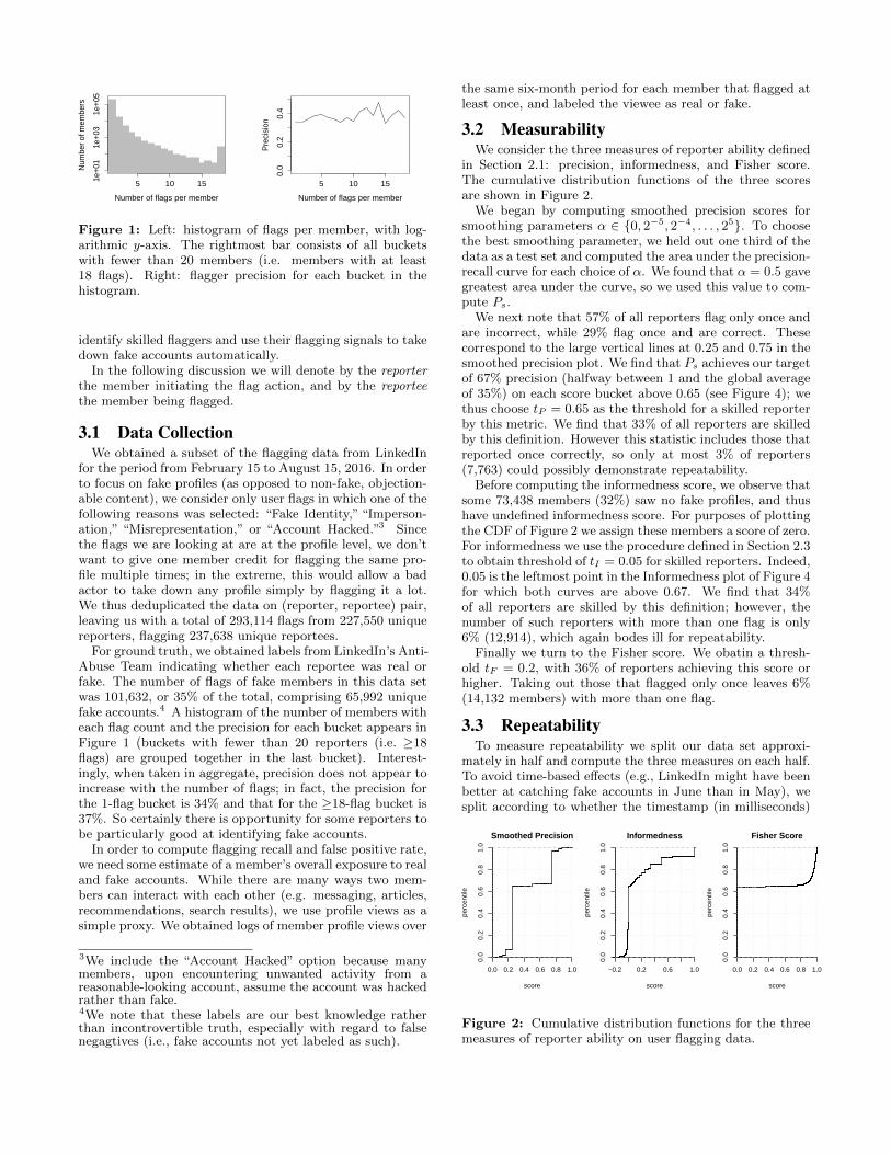
Figure 1: Left: histogram of flags per member, with log-arithmic y-axis. The rightmost bar consists of all bucketswith fewer than 20 members (i.e. members with at least18 flags). Right: flagger precision for each bucket in thehistogram.

identify skilled flaggers and use their flagging signals to takedown fake accounts automatically.

In the following discussion we will denote by the reporterthe member initiating the flag action, and by the reporteethe member being flagged.

3.1 Data CollectionWe obtained a subset of the flagging data from LinkedIn

for the period from February 15 to August 15, 2016. In orderto focus on fake profiles (as opposed to non-fake, objection-able content), we consider only user flags in which one of thefollowing reasons was selected: “Fake Identity,” “Imperson-ation,” “Misrepresentation,” or “Account Hacked.”3 Sincethe flags we are looking at are at the profile level, we don’twant to give one member credit for flagging the same pro-file multiple times; in the extreme, this would allow a badactor to take down any profile simply by flagging it a lot.We thus deduplicated the data on (reporter, reportee) pair,leaving us with a total of 293,114 flags from 227,550 uniquereporters, flagging 237,638 unique reportees.

For ground truth, we obtained labels from LinkedIn’s Anti-Abuse Team indicating whether each reportee was real orfake. The number of flags of fake members in this data setwas 101,632, or 35% of the total, comprising 65,992 uniquefake accounts.4 A histogram of the number of members witheach flag count and the precision for each bucket appears inFigure 1 (buckets with fewer than 20 reporters (i.e. ≥18flags) are grouped together in the last bucket). Interest-ingly, when taken in aggregate, precision does not appear toincrease with the number of flags; in fact, the precision forthe 1-flag bucket is 34% and that for the ≥18-flag bucket is37%. So certainly there is opportunity for some reporters tobe particularly good at identifying fake accounts.

In order to compute flagging recall and false positive rate,we need some estimate of a member’s overall exposure to realand fake accounts. While there are many ways two mem-bers can interact with each other (e.g. messaging, articles,recommendations, search results), we use profile views as asimple proxy. We obtained logs of member profile views over

3We include the “Account Hacked” option because manymembers, upon encountering unwanted activity from areasonable-looking account, assume the account was hackedrather than fake.4We note that these labels are our best knowledge ratherthan incontrovertible truth, especially with regard to falsenegagtives (i.e., fake accounts not yet labeled as such).

the same six-month period for each member that flagged atleast once, and labeled the viewee as real or fake.

3.2 MeasurabilityWe consider the three measures of reporter ability defined

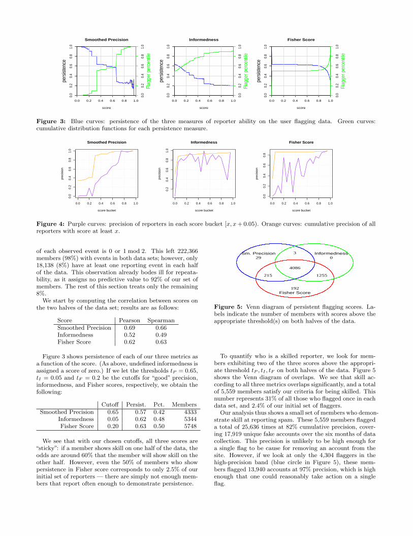
in Section 2.1: precision, informedness, and Fisher score.The cumulative distribution functions of the three scoresare shown in Figure 2.

We began by computing smoothed precision scores forsmoothing parameters α ∈ {0, 2−5, 2−4, . . . , 25}. To choosethe best smoothing parameter, we held out one third of thedata as a test set and computed the area under the precision-recall curve for each choice of α. We found that α = 0.5 gavegreatest area under the curve, so we used this value to com-pute Ps.

We next note that 57% of all reporters flag only once andare incorrect, while 29% flag once and are correct. Thesecorrespond to the large vertical lines at 0.25 and 0.75 in thesmoothed precision plot. We find that Ps achieves our targetof 67% precision (halfway between 1 and the global averageof 35%) on each score bucket above 0.65 (see Figure 4); wethus choose tP = 0.65 as the threshold for a skilled reporterby this metric. We find that 33% of all reporters are skilledby this definition. However this statistic includes those thatreported once correctly, so only at most 3% of reporters(7,763) could possibly demonstrate repeatability.

Before computing the informedness score, we observe thatsome 73,438 members (32%) saw no fake profiles, and thushave undefined informedness score. For purposes of plottingthe CDF of Figure 2 we assign these members a score of zero.For informedness we use the procedure defined in Section 2.3to obtain threshold of tI = 0.05 for skilled reporters. Indeed,0.05 is the leftmost point in the Informedness plot of Figure 4for which both curves are above 0.67. We find that 34%of all reporters are skilled by this definition; however, thenumber of such reporters with more than one flag is only6% (12,914), which again bodes ill for repeatability.

Finally we turn to the Fisher score. We obatin a thresh-old tF = 0.2, with 36% of reporters achieving this score orhigher. Taking out those that flagged only once leaves 6%(14,132 members) with more than one flag.

3.3 RepeatabilityTo measure repeatability we split our data set approxi-

mately in half and compute the three measures on each half.To avoid time-based effects (e.g., LinkedIn might have beenbetter at catching fake accounts in June than in May), wesplit according to whether the timestamp (in milliseconds)

0.0 0.2 0.4 0.6 0.8 1.0

0.0

0.2

0.4

0.6

0.8

1.0

Smoothed Precision

score

perc

entil

e

−0.2 0.2 0.6 1.0

0.0

0.2

0.4

0.6

0.8

1.0

Informedness

score

perc

entil

e

0.0 0.2 0.4 0.6 0.8 1.0

0.0

0.2

0.4

0.6

0.8

1.0

Fisher Score

score

perc

entil

e

Figure 2: Cumulative distribution functions for the threemeasures of reporter ability on user flagging data.

0.0 0.2 0.4 0.6 0.8 1.0

0.0

0.2

0.4

0.6

0.8

1.0

Smoothed Precision

score

pers

iste

nce

0.0

0.2

0.4

0.6

0.8

1.0

Flag

ger p

erce

ntile

0.0 0.2 0.4 0.6 0.8 1.0

0.0

0.2

0.4

0.6

0.8

1.0

Informedness

score

pers

iste

nce

0.0

0.2

0.4

0.6

0.8

1.0

Flag

ger p

erce

ntile

0.0 0.2 0.4 0.6 0.8 1.0

0.0

0.2

0.4

0.6

0.8

1.0

Fisher Score

score

pers

iste

nce

0.0

0.2

0.4

0.6

0.8

1.0

Flag

ger p

erce

ntile

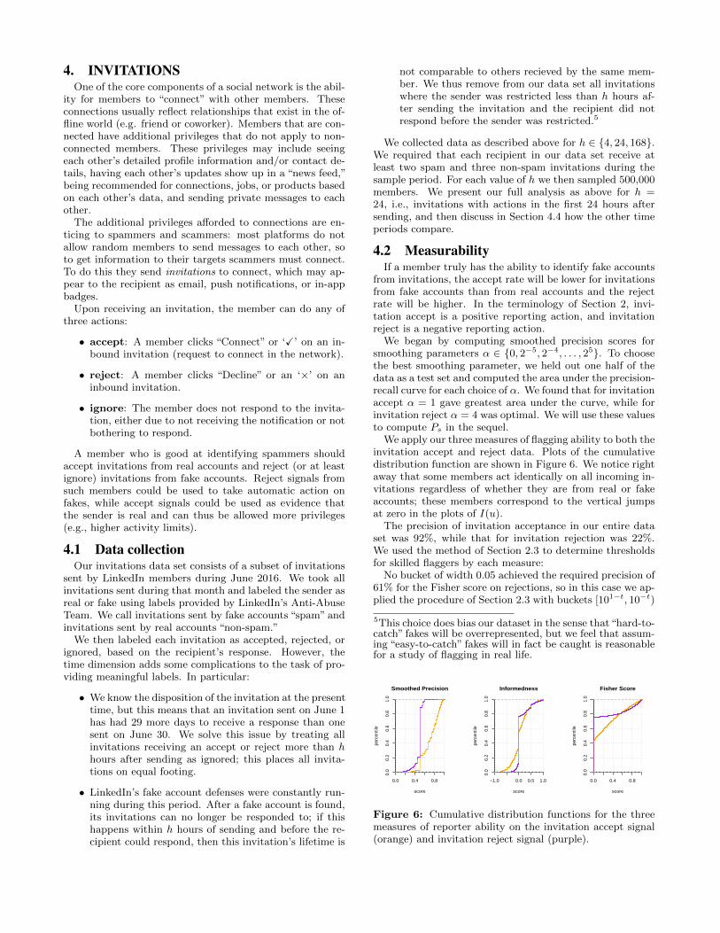
Figure 3: Blue curves: persistence of the three measures of reporter ability on the user flagging data. Green curves:cumulative distribution functions for each persistence measure.

0.0 0.2 0.4 0.6 0.8 1.0

0.0

0.2

0.4

0.6

0.8

1.0

Smoothed Precision

score bucket

prec

isio

n

0.0 0.2 0.4 0.6 0.8 1.0

0.2

0.4

0.6

0.8

1.0

Informedness

score bucket

prec

isio

n

0.0 0.2 0.4 0.6 0.8 1.0

0.0

0.2

0.4

0.6

0.8

Fisher Score

score bucket

prec

isio

n

Figure 4: Purple curves: precision of reporters in each score bucket [x, x+ 0.05). Orange curves: cumulative precision of allreporters with score at least x.

of each observed event is 0 or 1 mod 2. This left 222,366members (98%) with events in both data sets; however, only18,138 (8%) have at least one reporting event in each halfof the data. This observation already bodes ill for repeata-bility, as it assigns no predictive value to 92% of our set ofmembers. The rest of this section treats only the remaining8%.

We start by computing the correlation between scores onthe two halves of the data set; results are as follows:

Score Pearson SpearmanSmoothed Precision 0.69 0.66Informedness 0.52 0.49Fisher Score 0.62 0.63

Figure 3 shows persistence of each of our three metrics asa function of the score. (As above, undefined informedness isassigned a score of zero.) If we let the thresholds tP = 0.65,tI = 0.05 and tF = 0.2 be the cutoffs for “good” precision,informedness, and Fisher scores, respectively, we obtain thefollowing:

Cutoff Persist. Pct. MembersSmoothed Precision 0.65 0.57 0.42 4333

Informedness 0.05 0.62 0.48 5344Fisher Score 0.20 0.63 0.50 5748

We see that with our chosen cutoffs, all three scores are“sticky”: if a member shows skill on one half of the data, theodds are around 60% that the member will show skill on theother half. However, even the 50% of members who showpersistence in Fisher score corresponds to only 2.5% of ourinitial set of reporters — there are simply not enough mem-bers that report often enough to demonstrate persistence.

293

0

215

4086

1255

192

Sm. Precision Informedness

Fisher Score

Figure 5: Venn diagram of persistent flagging scores. La-bels indicate the number of members with scores above theappropriate threshold(s) on both halves of the data.

To quantify who is a skilled reporter, we look for mem-bers exhibiting two of the three scores above the appropri-ate threshold tP , tI , tF on both halves of the data. Figure 5shows the Venn diagram of overlaps. We see that skill ac-cording to all three metrics overlaps significantly, and a totalof 5,559 members satisfy our criteria for being skilled. Thisnumber represents 31% of all those who flagged once in eachdata set, and 2.4% of our initial set of flaggers.

Our analysis thus shows a small set of members who demon-strate skill at reporting spam. These 5,559 members flaggeda total of 25,636 times at 82% cumulative precision, cover-ing 17,919 unique fake accounts over the six months of datacollection. This precision is unlikely to be high enough fora single flag to be cause for removing an account from thesite. However, if we look at only the 4,304 flaggers in thehigh-precision band (blue circle in Figure 5), these mem-bers flagged 13,940 accounts at 97% precision, which is highenough that one could reasonably take action on a singleflag.

4. INVITATIONSOne of the core components of a social network is the abil-

ity for members to “connect” with other members. Theseconnections usually reflect relationships that exist in the of-fline world (e.g. friend or coworker). Members that are con-nected have additional privileges that do not apply to non-connected members. These privileges may include seeingeach other’s detailed profile information and/or contact de-tails, having each other’s updates show up in a “news feed,”being recommended for connections, jobs, or products basedon each other’s data, and sending private messages to eachother.

The additional privileges afforded to connections are en-ticing to spammers and scammers: most platforms do notallow random members to send messages to each other, soto get information to their targets scammers must connect.To do this they send invitations to connect, which may ap-pear to the recipient as email, push notifications, or in-appbadges.

Upon receiving an invitation, the member can do any ofthree actions:

• accept: A member clicks “Connect” or ‘X’ on an in-bound invitation (request to connect in the network).

• reject: A member clicks “Decline” or an ‘×’ on aninbound invitation.

• ignore: The member does not respond to the invita-tion, either due to not receiving the notification or notbothering to respond.

A member who is good at identifying spammers shouldaccept invitations from real accounts and reject (or at leastignore) invitations from fake accounts. Reject signals fromsuch members could be used to take automatic action onfakes, while accept signals could be used as evidence thatthe sender is real and can thus be allowed more privileges(e.g., higher activity limits).

4.1 Data collectionOur invitations data set consists of a subset of invitations

sent by LinkedIn members during June 2016. We took allinvitations sent during that month and labeled the sender asreal or fake using labels provided by LinkedIn’s Anti-AbuseTeam. We call invitations sent by fake accounts “spam” andinvitations sent by real accounts “non-spam.”

We then labeled each invitation as accepted, rejected, orignored, based on the recipient’s response. However, thetime dimension adds some complications to the task of pro-viding meaningful labels. In particular:

• We know the disposition of the invitation at the presenttime, but this means that an invitation sent on June 1has had 29 more days to receive a response than onesent on June 30. We solve this issue by treating allinvitations receiving an accept or reject more than hhours after sending as ignored; this places all invita-tions on equal footing.

• LinkedIn’s fake account defenses were constantly run-ning during this period. After a fake account is found,its invitations can no longer be responded to; if thishappens within h hours of sending and before the re-cipient could respond, then this invitation’s lifetime is

not comparable to others recieved by the same mem-ber. We thus remove from our data set all invitationswhere the sender was restricted less than h hours af-ter sending the invitation and the recipient did notrespond before the sender was restricted.5

We collected data as described above for h ∈ {4, 24, 168}.We required that each recipient in our data set receive atleast two spam and three non-spam invitations during thesample period. For each value of h we then sampled 500,000members. We present our full analysis as above for h =24, i.e., invitations with actions in the first 24 hours aftersending, and then discuss in Section 4.4 how the other timeperiods compare.

4.2 MeasurabilityIf a member truly has the ability to identify fake accounts

from invitations, the accept rate will be lower for invitationsfrom fake accounts than from real accounts and the rejectrate will be higher. In the terminology of Section 2, invi-tation accept is a positive reporting action, and invitationreject is a negative reporting action.

We began by computing smoothed precision scores forsmoothing parameters α ∈ {0, 2−5, 2−4, . . . , 25}. To choosethe best smoothing parameter, we held out one half of thedata as a test set and computed the area under the precision-recall curve for each choice of α. We found that for invitationaccept α = 1 gave greatest area under the curve, while forinvitation reject α = 4 was optimal. We will use these valuesto compute Ps in the sequel.

We apply our three measures of flagging ability to both theinvitation accept and reject data. Plots of the cumulativedistribution function are shown in Figure 6. We notice rightaway that some members act identically on all incoming in-vitations regardless of whether they are from real or fakeaccounts; these members correspond to the vertical jumpsat zero in the plots of I(u).

The precision of invitation acceptance in our entire dataset was 92%, while that for invitation rejection was 22%.We used the method of Section 2.3 to determine thresholdsfor skilled flaggers by each measure:

No bucket of width 0.05 achieved the required precision of61% for the Fisher score on rejections, so in this case we ap-plied the procedure of Section 2.3 with buckets [101−t, 10−t)

5This choice does bias our dataset in the sense that“hard-to-catch” fakes will be overrepresented, but we feel that assum-ing “easy-to-catch” fakes will in fact be caught is reasonablefor a study of flagging in real life.

0.0 0.4 0.8

0.0

0.2

0.4

0.6

0.8

1.0

Smoothed Precision

score

perc

entil

e

−1.0 0.0 0.5 1.0

0.0

0.2

0.4

0.6

0.8

1.0

Informedness

score

perc

entil

e

0.0 0.4 0.8

0.0

0.2

0.4

0.6

0.8

1.0

Fisher Score

score

perc

entil

e

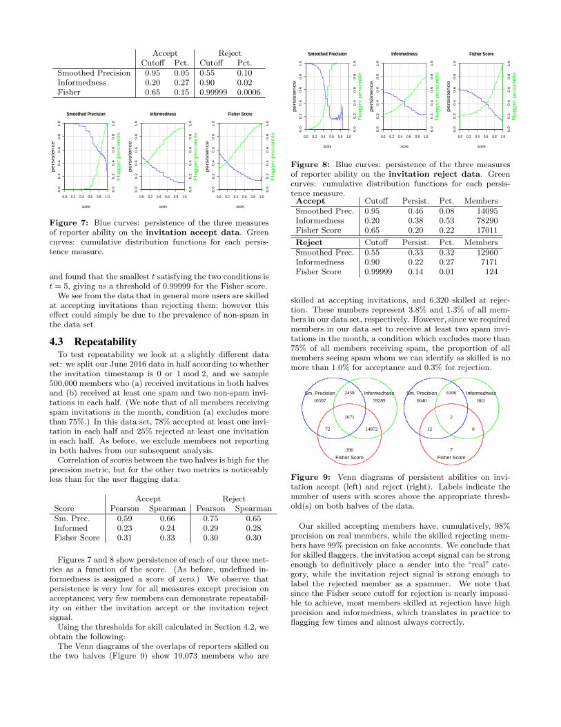
Figure 6: Cumulative distribution functions for the threemeasures of reporter ability on the invitation accept signal(orange) and invitation reject signal (purple).

Accept RejectCutoff Pct. Cutoff Pct.

Smoothed Precision 0.95 0.05 0.55 0.10Informedness 0.20 0.27 0.90 0.02Fisher 0.65 0.15 0.99999 0.0006

0.0 0.2 0.4 0.6 0.8 1.0

0.0

0.2

0.4

0.6

0.8

1.0

Smoothed Precision

score

pe

rsis

ten

ce

0.0

0.2

0.4

0.6

0.8

1.0

Fla

gg

er

pe

rce

ntile

0.0 0.2 0.4 0.6 0.8 1.0

0.0

0.2

0.4

0.6

0.8

1.0

Informedness

score

pe

rsis

ten

ce

0.0

0.2

0.4

0.6

0.8

1.0

Fla

gg

er

pe

rce

ntile

0.0 0.2 0.4 0.6 0.8 1.0

0.0

0.2

0.4

0.6

0.8

1.0

Fisher Score

scorep

ers

iste

nce

0.0

0.2

0.4

0.6

0.8

1.0

Fla

gg

er

pe

rce

ntile

Figure 7: Blue curves: persistence of the three measuresof reporter ability on the invitation accept data. Greencurves: cumulative distribution functions for each persis-tence measure.

and found that the smallest t satisfying the two conditions ist = 5, giving us a threshold of 0.99999 for the Fisher score.

We see from the data that in general more users are skilledat accepting invitations than rejecting them; however thiseffect could simply be due to the prevalence of non-spam inthe data set.

4.3 RepeatabilityTo test repeatability we look at a slightly different data

set: we split our June 2016 data in half according to whetherthe invitation timestamp is 0 or 1 mod 2, and we sample500,000 members who (a) received invitations in both halvesand (b) received at least one spam and two non-spam invi-tations in each half. (We note that of all members receivingspam invitations in the month, condition (a) excludes morethan 75%.) In this data set, 78% accepted at least one invi-tation in each half and 25% rejected at least one invitationin each half. As before, we exclude members not reportingin both halves from our subsequent analysis.

Correlation of scores between the two halves is high for theprecision metric, but for the other two metrics is noticeablyless than for the user flagging data:

Accept RejectScore Pearson Spearman Pearson SpearmanSm. Prec. 0.59 0.66 0.75 0.65Informed 0.23 0.24 0.29 0.28Fisher Score 0.31 0.33 0.30 0.30

Figures 7 and 8 show persistence of each of our three met-rics as a function of the score. (As before, undefined in-formedness is assigned a score of zero.) We observe thatpersistence is very low for all measures except precision onacceptances; very few members can demonstrate repeatabil-ity on either the invitation accept or the invitation rejectsignal.

Using the thresholds for skill calculated in Section 4.2, weobtain the following:

The Venn diagrams of the overlaps of reporters skilled onthe two halves (Figure 9) show 19,073 members who are

0.0 0.2 0.4 0.6 0.8 1.0

0.0

0.2

0.4

0.6

0.8

1.0

Smoothed Precision

score

pe

rsis

ten

ce

0.0

0.2

0.4

0.6

0.8

1.0

Fla

gg

er

pe

rce

ntile

0.0 0.2 0.4 0.6 0.8 1.0

0.0

0.2

0.4

0.6

0.8

1.0

Informedness

score

pe

rsis

ten

ce

0.0

0.2

0.4

0.6

0.8

1.0

Fla

gg

er

pe

rce

ntile

0.0 0.2 0.4 0.6 0.8 1.0

0.0

0.2

0.4

0.6

0.8

1.0

Fisher Score

score

pe

rsis

ten

ce

0.0

0.2

0.4

0.6

0.8

1.0

Fla

gg

er

pe

rce

ntile

Figure 8: Blue curves: persistence of the three measuresof reporter ability on the invitation reject data. Greencurves: cumulative distribution functions for each persis-tence measure.Accept Cutoff Persist. Pct. MembersSmoothed Prec. 0.95 0.46 0.08 14095Informedness 0.20 0.38 0.53 78290Fisher Score 0.65 0.20 0.22 17011

Reject Cutoff Persist. Pct. MembersSmoothed Prec. 0.55 0.33 0.32 12960Informedness 0.90 0.22 0.27 7171Fisher Score 0.99999 0.14 0.01 124

skilled at accepting invitations, and 6,320 skilled at rejec-tion. These numbers represent 3.8% and 1.3% of all mem-bers in our data set, respectively. However, since we requiredmembers in our data set to receive at least two spam invi-tations in the month, a condition which excludes more than75% of all members receiving spam, the proportion of allmembers seeing spam whom we can identify as skilled is nomore than 1.0% for acceptance and 0.3% for rejection.

10597

2458

59289

72

1671

14872

396

Sm. Precision Informedness

Fisher Score

6640

6306

863

12

2

0

7

Sm. Precision Informedness

Fisher Score

Figure 9: Venn diagrams of persistent abilities on invi-tation accept (left) and reject (right). Labels indicate thenumber of users with scores above the appropriate thresh-old(s) on both halves of the data.

Our skilled accepting members have, cumulatively, 98%precision on real members, while the skilled rejecting mem-bers have 99% precision on fake accounts. We conclude thatfor skilled flaggers, the invitation accept signal can be strongenough to definitively place a sender into the “real” cate-gory, while the invitation reject signal is strong enough tolabel the rejected member as a spammer. We note thatsince the Fisher score cutoff for rejection is nearly impossi-ble to achieve, most members skilled at rejection have highprecision and informedness, which translates in practice toflagging few times and almost always correctly.

0.0 0.2 0.4 0.6 0.8 1.0

0.0

0.2

0.4

0.6

0.8

1.0

Invitation Accept

score

perc

entil

e

0.0 0.2 0.4 0.6 0.8 1.0

0.0

0.2

0.4

0.6

0.8

1.0

Invitation Reject

score

perc

entil

e

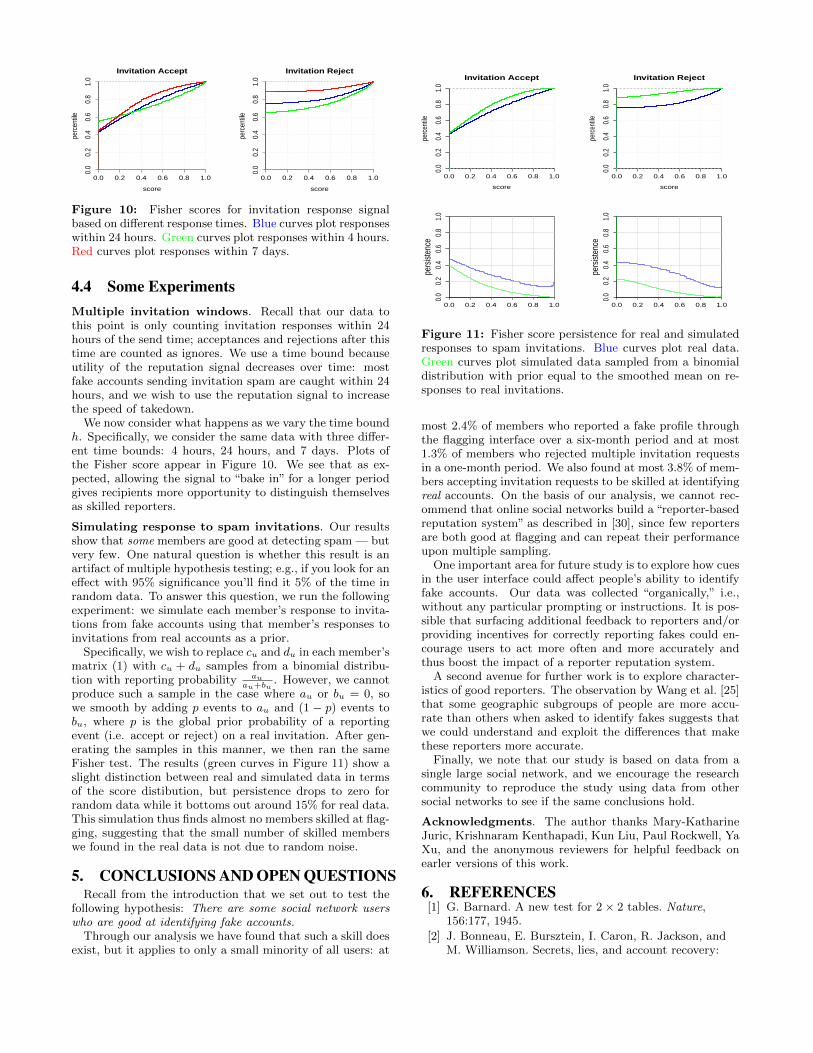
Figure 10: Fisher scores for invitation response signalbased on different response times. Blue curves plot responseswithin 24 hours. Green curves plot responses within 4 hours.Red curves plot responses within 7 days.

4.4 Some ExperimentsMultiple invitation windows. Recall that our data tothis point is only counting invitation responses within 24hours of the send time; acceptances and rejections after thistime are counted as ignores. We use a time bound becauseutility of the reputation signal decreases over time: mostfake accounts sending invitation spam are caught within 24hours, and we wish to use the reputation signal to increasethe speed of takedown.

We now consider what happens as we vary the time boundh. Specifically, we consider the same data with three differ-ent time bounds: 4 hours, 24 hours, and 7 days. Plots ofthe Fisher score appear in Figure 10. We see that as ex-pected, allowing the signal to “bake in” for a longer periodgives recipients more opportunity to distinguish themselvesas skilled reporters.

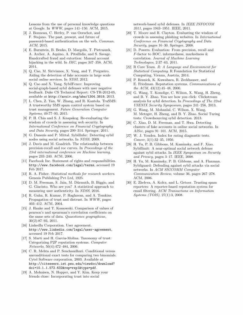
Simulating response to spam invitations. Our resultsshow that some members are good at detecting spam — butvery few. One natural question is whether this result is anartifact of multiple hypothesis testing; e.g., if you look for aneffect with 95% significance you’ll find it 5% of the time inrandom data. To answer this question, we run the followingexperiment: we simulate each member’s response to invita-tions from fake accounts using that member’s responses toinvitations from real accounts as a prior.

Specifically, we wish to replace cu and du in each member’smatrix (1) with cu + du samples from a binomial distribu-tion with reporting probability au

au+bu. However, we cannot

produce such a sample in the case where au or bu = 0, sowe smooth by adding p events to au and (1 − p) events tobu, where p is the global prior probability of a reportingevent (i.e. accept or reject) on a real invitation. After gen-erating the samples in this manner, we then ran the sameFisher test. The results (green curves in Figure 11) show aslight distinction between real and simulated data in termsof the score distibution, but persistence drops to zero forrandom data while it bottoms out around 15% for real data.This simulation thus finds almost no members skilled at flag-ging, suggesting that the small number of skilled memberswe found in the real data is not due to random noise.

5. CONCLUSIONS AND OPEN QUESTIONSRecall from the introduction that we set out to test the

following hypothesis: There are some social network userswho are good at identifying fake accounts.

Through our analysis we have found that such a skill doesexist, but it applies to only a small minority of all users: at

0.0 0.2 0.4 0.6 0.8 1.0

0.0

0.2

0.4

0.6

0.8

1.0

Invitation Accept

score

perc

entile

0.0 0.2 0.4 0.6 0.8 1.0

0.0

0.2

0.4

0.6

0.8

1.0

Invitation Reject

score

perc

entile

0.0 0.2 0.4 0.6 0.8 1.0

0.0

0.2

0.4

0.6

0.8

1.0

score

pers

isten

ce

0.0 0.2 0.4 0.6 0.8 1.0

0.0

0.2

0.4

0.6

0.8

1.0

score

pers

isten

ce

Figure 11: Fisher score persistence for real and simulatedresponses to spam invitations. Blue curves plot real data.Green curves plot simulated data sampled from a binomialdistribution with prior equal to the smoothed mean on re-sponses to real invitations.

most 2.4% of members who reported a fake profile throughthe flagging interface over a six-month period and at most1.3% of members who rejected multiple invitation requestsin a one-month period. We also found at most 3.8% of mem-bers accepting invitation requests to be skilled at identifyingreal accounts. On the basis of our analysis, we cannot rec-ommend that online social networks build a “reporter-basedreputation system” as described in [30], since few reportersare both good at flagging and can repeat their performanceupon multiple sampling.

One important area for future study is to explore how cuesin the user interface could affect people’s ability to identifyfake accounts. Our data was collected “organically,” i.e.,without any particular prompting or instructions. It is pos-sible that surfacing additional feedback to reporters and/orproviding incentives for correctly reporting fakes could en-courage users to act more often and more accurately andthus boost the impact of a reporter reputation system.

A second avenue for further work is to explore character-istics of good reporters. The observation by Wang et al. [25]that some geographic subgroups of people are more accu-rate than others when asked to identify fakes suggests thatwe could understand and exploit the differences that makethese reporters more accurate.

Finally, we note that our study is based on data from asingle large social network, and we encourage the researchcommunity to reproduce the study using data from othersocial networks to see if the same conclusions hold.

Acknowledgments. The author thanks Mary-KatharineJuric, Krishnaram Kenthapadi, Kun Liu, Paul Rockwell, YaXu, and the anonymous reviewers for helpful feedback onearler versions of this work.

6. REFERENCES[1] G. Barnard. A new test for 2× 2 tables. Nature,

156:177, 1945.

[2] J. Bonneau, E. Bursztein, I. Caron, R. Jackson, andM. Williamson. Secrets, lies, and account recovery:

Lessons from the use of personal knowledge questionsat Google. In WWW, pages 141–150. ACM, 2015.

[3] J. Bonneau, C. Herley, P. van Oorschot, andF. Stajano. The past, present, and future ofpassword-based authentication on the web. Commun.ACM, 2015.

[4] E. Bursztein, B. Benko, D. Margolis, T. Pietraszek,A. Archer, A. Aquino, A. Pitsillidis, and S. Savage.Handcrafted fraud and extortion: Manual accounthijacking in the wild. In IMC, pages 347–358. ACM,2014.

[5] Q. Cao, M. Sirivianos, X. Yang, and T. Pregueiro.Aiding the detection of fake accounts in large scalesocial online services. In NDSI, 2012.

[6] Q. Cao and X. Yang. SybilFence: Improvingsocial-graph-based sybil defenses with user negativefeedback. Duke CS Technical Report: CS-TR-2012-05,available at http://arxiv.org/abs/1304.3819, 2013.

[7] L. Chen, Z. Yan, W. Zhang, and R. Kantola. TruSMS:A trustworthy SMS spam control system based ontrust management. Future Generation ComputerSystems, 49:77–93, 2015.

[8] P. H. Chia and S. J. Knapskog. Re-evaluating thewisdom of crowds in assessing web security. InInternational Conference on Financial Cryptographyand Data Security, pages 299–314. Springer, 2011.

[9] G. Danezis and P. Mittal. SybilInfer: Detecting sybilnodes using social networks. In NDSS, 2009.

[10] J. Davis and M. Goadrich. The relationship betweenprecision-recall and roc curves. In Proceedings of the23rd international conference on Machine learning,pages 233–240. ACM, 2006.

[11] Facebook Inc. Statement of rights and responsibilities.http://www.facebook.com/legal/terms, accessed 19Feb 2017.

[12] R. A. Fisher. Statistical methods for research workers.Genesis Publishing Pvt Ltd, 1925.

[13] D. M. Freeman, S. Jain, M. Durmuth, B. Biggio, andG. Giacinto. Who are you? A statistical approach tomeasuring user authenticity. In NDSS, 2016.

[14] R. Guha, R. Kumar, P. Raghavan, and A. Tomkins.Propagation of trust and distrust. In WWW, pages403–412. ACM, 2004.

[15] J. Hauke and T. Kossowski. Comparison of values ofpearson’s and spearman’s correlation coefficients onthe same sets of data. Quaestiones geographicae,30(2):87–93, 2011.

[16] LinkedIn Corporation. User agreement.http://www.linkedin.com/legal/user-agreement,accessed 19 Feb 2017.

[17] S. Marti and H. Garcia-Molina. Taxonomy of trust:Categorizing P2P reputation systems. ComputerNetworks, 50(4):472–484, 2006.

[18] C. R. Mehta and P. Senchaudhuri. Conditional versusunconditional exact tests for comparing two binomials.Cytel Software corporation, 2003. Available athttp://citeseerx.ist.psu.edu/viewdoc/download?

doi=10.1.1.572.632&rep=rep1&type=pdf.

[19] A. Mohaisen, N. Hopper, and Y. Kim. Keep yourfriends close: Incorporating trust into social

network-based sybil defenses. In IEEE INFOCOM2011, pages 1943–1951. IEEE, 2011.

[20] T. Moore and R. Clayton. Evaluating the wisdom ofcrowds in assessing phishing websites. In InternationalConference on Financial Cryptography and DataSecurity, pages 16–30. Springer, 2008.

[21] D. Powers. Evaluation: From precision, recall andF -factor to ROC, informedness, markedness &correlation. Journal of Machine LearningTechnologies, 2:37–63, 2011.

[22] R Core Team. R: A Language and Environment forStatistical Computing. R Foundation for StatisticalComputing, Vienna, Austria, 2014.

[23] P. Resnick, K. Kuwabara, R. Zeckhauser, andE. Friedman. Reputation systems. Communications ofthe ACM, 43(12):45–48, 2000.

[24] G. Wang, T. Konolige, C. Wilson, X. Wang, H. Zheng,and B. Y. Zhao. You are how you click: Clickstreamanalysis for sybil detection. In Proceedings of The 22ndUSENIX Security Symposium, pages 241–256, 2013.

[25] G. Wang, M. Mohanlal, C. Wilson, X. Wang,M. Metzger, H. Zheng, and B. Y. Zhao. Social Turingtests: Crowdsourcing sybil detection. 2013.

[26] C. Xiao, D. M. Freeman, and T. Hwa. Detectingclusters of fake accounts in online social networks. InAISec, pages 91–101. ACM, 2015.

[27] W. J. Youden. Index for rating diagnostic tests.Cancer, 3(1):32–35, 1950.

[28] H. Yu, P. B. Gibbons, M. Kaminsky, and F. Xiao.Sybillimit: A near-optimal social network defenseagainst sybil attacks. In IEEE Symposium on Securityand Privacy, pages 3–17. IEEE, 2008.

[29] H. Yu, M. Kaminsky, P. B. Gibbons, and A. Flaxman.Sybilguard: Defending against sybil attacks via socialnetworks. In ACM SIGCOMM ComputerCommunication Review, volume 36, pages 267–278.ACM, 2006.

[30] E. Zheleva, A. Kolcz, and L. Getoor. Trusting spamreporters: A reporter-based reputation system foremail filtering. ACM Transactions on InformationSystems (TOIS), 27(1):3, 2008.