can we reach the zeptouniverse with rare and s;d decays? · can we reach the zeptouniverse with...
TRANSCRIPT
FLAVOUR(267104)-ERC-75
Can we reach the Zeptouniverse withrare K and Bs,d decays?
Andrzej J. Buras, Dario Buttazzo,Jennifer Girrbach-Noe and Robert Knegjens
TUM Institute for Advanced Study, Lichtenbergstraße 2a, 85748 Garching, Germany
Physik Department TUM, James-Franck-Straße, 85748 Garching, Germany
Abstract
The Large Hadron Collider (LHC) will directly probe distance scales as short as10−19 m, corresponding to energy scales at the level of a few TeV. In order toreach even higher resolutions before the advent of future high-energy colliders, itis necessary to consider indirect probes of New Physics (NP), a prime examplebeing ∆F = 2 neutral meson mixing processes, which are sensitive to much shorterdistance scales. However ∆F = 2 processes alone cannot tell us much about thestructure of NP beyond the LHC scales. To identify for instance the presence ofnew quark flavour-changing dynamics of a left-handed (LH) or right-handed (RH)nature, complementary results from ∆F = 1 rare decay processes are vital. Wetherefore address the important question of whether NP could be seen up to energyscales as high as 200 TeV, corresponding to distances as small as O(10−21) – theZeptouniverse – in rare K and Bs,d decays, subject to present ∆F = 2 constraintsand perturbativity. We focus in particular on a heavy Z ′ gauge boson. If restrictedto purely LH or RH Z ′ couplings to quarks, we find that rare K decays, in particularK+ → π+νν̄ and KL → π0νν̄, allow us to probe the Zeptouniverse. On the otherhand rare Bs and Bd decays, which receive stronger ∆F = 2 constraints, allow usto reach about 15 TeV. Allowing for both LH and RH couplings a loosening of the∆F = 2 constraints is possible, and we find that the maximal values of MZ′ atwhich NP effects could be found that are consistent with perturbative couplings areapproximately 2000 TeV for K decays and 160 TeV for rare Bs,d decays. Because Z ′
exchanges in the Bs,d → µ+µ− rare decays are helicity suppressed, we also considertree-level scalar exchanges for these decays, for which we find that scales close to1000 TeV can be probed for the analogous pure and combined LH and RH scenarios.We further present a simple idea for an indirect determination of MZ′ that couldbe realised at the next linear e+e− or µ+µ− collider and with future precise flavourdata.
arX
iv:1
408.
0728
v2 [
hep-
ph]
29
Oct
201
4
1 Introduction 1
Contents
1 Introduction 1
2 Setup and strategy 3
3 Left-handed and right-handed Z′ scenarios 53.1 Left-handed scenario . . . . . . . . . . . . . . . . . . . . . . . . 53.2 Right-handed scenario . . . . . . . . . . . . . . . . . . . . . . . . 113.3 Numerical analysis . . . . . . . . . . . . . . . . . . . . . . . . . 11
4 Left-Right operators at work 154.1 Basic idea . . . . . . . . . . . . . . . . . . . . . . . . . . . . . . 154.2 L+R scenario . . . . . . . . . . . . . . . . . . . . . . . . . . . . 164.3 Numerical analysis . . . . . . . . . . . . . . . . . . . . . . . . . 20
5 The case of a neutral scalar or pseudoscalar 225.1 Preliminaries . . . . . . . . . . . . . . . . . . . . . . . . . . . . 225.2 General formulae . . . . . . . . . . . . . . . . . . . . . . . . . . 235.3 Left-handed and right-handed scalar scenarios . . . . . . . . . . . 255.4 L+R scalar scenario . . . . . . . . . . . . . . . . . . . . . . . . . 26
6 Other New Physics scenarios 276.1 Preliminaries . . . . . . . . . . . . . . . . . . . . . . . . . . . . 276.2 The case of two gauge bosons . . . . . . . . . . . . . . . . . . . . 276.3 The case of a degenerate scalar and pseudo-scalar pair . . . . . . . 286.4 GIM case . . . . . . . . . . . . . . . . . . . . . . . . . . . . . . 29
7 Can we determine MZ′ beyond the LHC scales? 29
8 Conclusions 30
A ∆F = 1 master functions 32
B Basic formulae for observables 33
References 35
1 Introduction
Through the recent discovery of the Higgs particle the Standard Model (SM) ofstrong and electroweak interactions is now complete, with the masses of all its par-ticles being below 200 GeV, corresponding to scales above one Attometer (10−18 m).With the help of the Large Hadron Collider (LHC) the second half of this decade,together with the next decade, should allow us to probe directly the existence ofother particles present in nature with masses up to a few TeV. Many models con-sidered in the literature predict new gauge bosons, new fermions and new scalarsin this mass range, but until now no clear signal of these new particles has beenseen at the LHC. It is still possible that with the increased energy at the LHC new
1 Introduction 2
discoveries will be made in the coming years. But what if the lightest new particlein nature is in the multi-TeV range and out of the direct reach of the LHC?
The past successes of flavour physics in predicting new particles prior to theirdiscovery may again help us in such a case, in particular in view of significantimprovements on the precision of experiments and significant reduction of hadronicuncertainties through lattice QCD. But the question arises whether we will everreach the energy scales as high as 200 TeV corresponding to short distances in theballpark of 10−21 m – the Zeptouniverse – in this manner and learn about the natureof New Physics (NP) at these very short distances.1 The scale of 200 TeV is givenhere only as an example, and learning about NP at any scale above the LHC scalein this manner would be very important. Recent reviews on flavour physics beyondthe SM can be found in [1, 2].
Some readers may ask why we are readdressing this question in view of the com-prehensive analyses in the framework of effective theories in [3–5]. These analyses,which dealt dominantly with ∆F = 2 observables, have already shown that in thepresence of left-right operators one could be in principle sensitive to scales as highas 104 TeV, or even higher scales. Here we would like to point out that the study ofsuch processes alone will not really give us significant information about the partic-ular nature of this NP. To this end also ∆F = 1 processes, in particular rare K andBs,d decays, have to be considered. As left-right operators involving four quarks arenot the driving force in these decays, which generally contain operators built out ofone quark current and one lepton current, it is not evident that these decays canhelp us in reaching the Zeptouniverse even in the flavour precision era. In fact aswill be evident from our analysis below, NP at scales well above 1000 TeV cannotbe probed by rare meson decays.2
In this paper we address this question primarily in the context of one of thesimplest extensions of the SM, a Z ′ model in which a heavy neutral gauge bosonmediates FCNC processes in the quark sector at tree-level and has left-handed (LH)and/or right-handed (RH) couplings to quarks and leptons. This model has beenstudied recently for the general case in [16, 17] and in [18–20] in the context of 331models. However, in these papers MZ′ has been chosen in the reach of the LHC,typically in the ballpark of 3 TeV. Here the philosophy will be to focus on thehighest mass scales possibly accessible through flavour measurements. It is evidentfrom [20] that in 331 models NP effects for MZ′ ≥ 10 TeV are too small to bemeasured in rare K and Bs,d decays even in the flavour precision era. On the otherhand, as we will see, this is still possible in a general Z ′ model. References to otheranalyses in Z ′ models are collected in [1].
The Z ′ model that we will analyze is only one possible NP scenario and shouldthereby be considered as a useful concrete example in which our questions canbe answered in explicit terms. It is nevertheless important to investigate whetherother NP scenarios could also give sufficiently strong signals from very short distancescales so that they could be detected in future measurements. If fact we find thattree-level scalar exchanges could also give us informations about these very shortscales through Bs,d → µ+µ− decays.
1We consider scales in the same ballpark, for example 50 TeV and 1000 TeV, which correspondrespectively to 4 and 0.2 zeptometers and also belong to the Zeptouniverse.
2In principle this could be achieved in the future with the help of lepton flavour violating decays suchas µ→ eγ and µ→ 3e, µ→ e conversion in nuclei, and electric dipole moments [6–15].
2 Setup and strategy 3
Our paper is organised as follows. In Section 2 we outline the strategy for findingthe maximal possible resolution of short distance scales with the help of rare mesondecays. This depends on the maximal value of the Z ′ couplings to fermions thatare allowed by perturbativity and present experimental constraints. It also dependson the minimal deviations from SM expectations that in the flavour precision eracould be considered as a clear signal of NP. In Section 3 we perform the analysisfor Z ′ scenarios with only LH or only RH flavour violating couplings to quarks.In Section 4 the case of Z ′ with LH and RH flavour violating couplings to quarksis analysed. In Section 5 we repeat the analysis of previous sections for tree-level(pseudo-)scalar contributions restricting the discussion to the decays Bs,d → µ+µ−.In Section 6 we discuss briefly other NP scenarios. In Section 7 we present a simpleidea for a rough indirect determination of MZ′ by means of the next linear e+e− orµ+µ− collider and flavour data. We conclude in Section 8.
2 Setup and strategy
The virtue of the Z ′ scenarios is the paucity of their parameters that enter allflavour observables in a given meson system, which should be contrasted with mostNP scenarios outside the Minimal Flavour Violation (MFV) framework. Indeed, the∆F = 2 and ∆F = 1 transitions in the K, Bd and Bs systems are fully describedby the following ratios of the Z ′ couplings to SM fermions over its mass MZ′ ,
∆sdL,R/MZ′ , ∆bd
L,R/MZ′ , ∆bsL,R/MZ′ , (1)
and
∆νν̄L /MZ′ , ∆µµ̄
A /MZ′ , ∆µµ̄V = 2∆νν̄
L + ∆µµ̄A , (2)
where the last formula follows from the SU(2)L symmetry relation ∆νν̄L = ∆µµ̄
L .These couplings are defined as in [16,17] through
LquarksFCNC =
[q̄i γµ PL qj ∆ij
L + q̄i γµ PR qj ∆ijR + h.c.
]Z ′µ, (3)
with i, j = d, s, b and i 6= j throughout the rest of the paper. The analogousdefinition applies to the lepton sector where only flavour conserving couplings areconsidered,
Lleptons =[µ̄ γµ PL µ∆µµ̄
L + µ̄ γµ PR µ∆µµ̄R + ν̄ γµ PL ∆νν̄
L
]Z ′µ . (4)
We recall that the couplings ∆µµ̄A,V are defined as
∆µµ̄V = ∆µµ̄
R + ∆µµ̄L , ∆µµ̄
A = ∆µµ̄R −∆µµ̄
L . (5)
Other definitions and normalisation of couplings can be found in [16]. The quarkcouplings are in general complex whereas the leptonic ones are assumed to be real.
It is evident from these expressions that in order to find out the maximal value ofMZ′ for which measurable NP effects in ∆F = 2 and ∆F = 1 exist one has to knowthe maximal values of the couplings ∆ij
L,R and ∆µµ̄L,R allowed by perturbativity. From
the ∆F = 2 analyses in [3–5] it follows that by choosing these couplings to be O(1)
2 Setup and strategy 4
the lower bound on the scale of new physics ΛNP could be in the range of 105 TeVfor the case of K0 − K̄0 mixing. On the other hand, choosing sufficiently smallcouplings by means of a suitable flavour symmetry it is possible to suppress theFCNCs related to NP with the NP scale ΛNP in the ballpark of a few TeV [21–28].
In view of the fact that flavour physics in the rest of this decade and in the nextdecade will be dominated by new precise measurements of rare K and rare Bs,ddecays and not ∆F = 2 transitions, our strategy will differ from the one in [3–5].We will assume that future measurements will be precise enough to identify conclu-sively the presence of NP in rare decays when the deviations from SM predictionsfor various branching ratios will be larger than 10 – 30% of the SM branching ratio.The precise value of the detectable deviation will depend on the decay consideredand will be smaller for the ones with smaller experimental, hadronic and parametricuncertainties. We will be more specific about this in the next section. The frame-work considered here goes beyond MFV, where even for ΛNP in the ballpark of a fewTeV only moderate departures from the SM in ∆F = 1 observables are predicted.A model independent analysis of b→ s transitions in this framework can be foundin [29] and in a recent review in [30].
In order to proceed we have to make assumptions about the size of the couplingsinvolved. There is in general a lot of freedom here, but as we are searching for themaximal values of MZ′ which could still provide measurable NP effects in rare mesondecays, we will choose maximal couplings that are consistent with perturbativity.Subsequently we will check whether such couplings are also consistent with ∆F = 2constraints for a given MZ′ . An estimate of the perturbativity upper bound on∆sdL,R was made in [31], in the context of a study of the isospin amplitude A0 in
K → ππ decays, by considering the loop expansion parameter
L = Nc
(∆sdL,R
4π
)2
, (6)
where Nc = 3 is the number of colours. For ∆sdL,R = 3.0 we find L = 0.17, a coupling
strength that is certainly allowed. The same estimate can be made for other LH andRH couplings considered by us. However, as we will see below, the correlation of∆F = 1 and ∆F = 2 processes in the case of Z ′ exchange, derived in [16], will givesome additional insight on the allowed size of the quark couplings and will generallynot allow us to reach the perturbativity bounds on quark couplings. On the otherhand, large values of the leptonic couplings ∆νν̄
L and ∆µµ̄V,A at the perturbativity
upper bound will give an estimate of the maximal MZ′ for which measurable effectsin rare K and Bs,d decays could be obtained.
In the case of a U(1) gauge symmetry with large gauge couplings at a given scaleit is difficult to avoid a Landau pole at still higher scales. However, for the couplingvalues used in our paper, this happens at much higher scales than MZ′ . Moreover,if Z ′ is associated with a non-abelian gauge symmetry that is asymptotically freethis problem does not exist.
Projections for the coming years
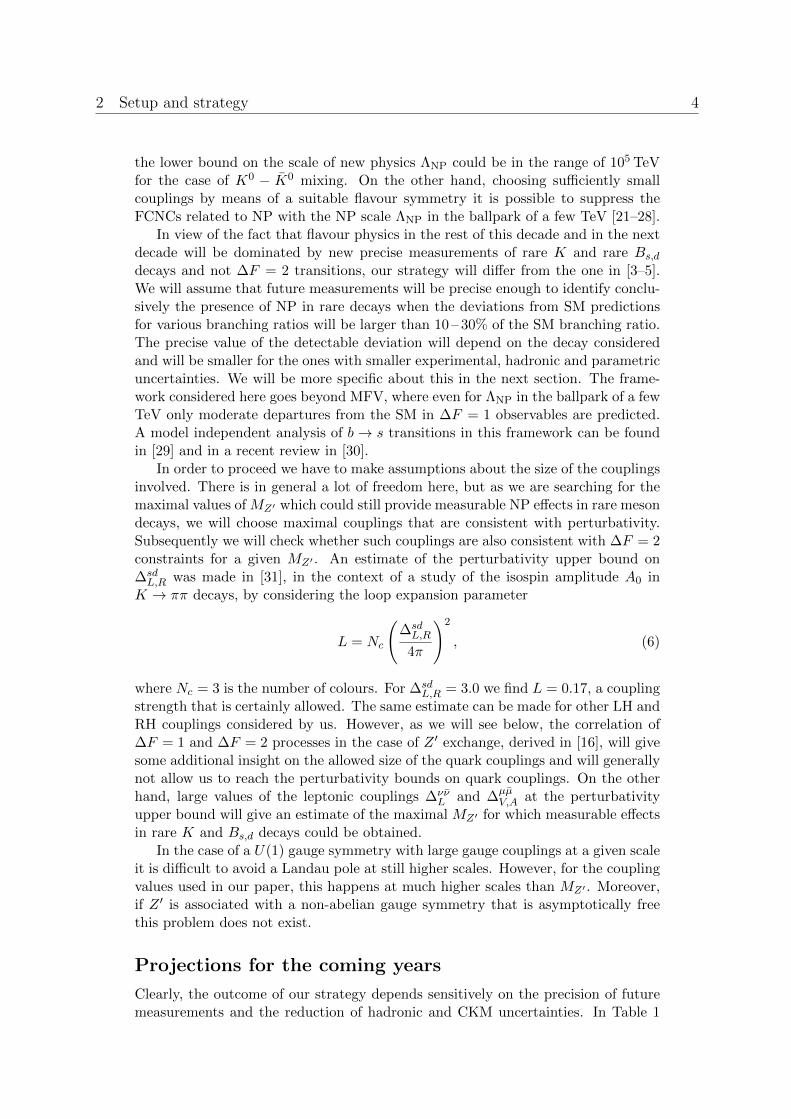
Clearly, the outcome of our strategy depends sensitively on the precision of futuremeasurements and the reduction of hadronic and CKM uncertainties. In Table 1
3 Left-handed and right-handed Z ′ scenarios 5
Observable 2014 2019 2024 2030
B(K+ → π+νν̄)(17.3+11.5
−10.5
)× 10−11 [32] 10% [33] 5% [34]
B(KL → π0νν̄) < 2.6× 10⁻⁸ (90% CL)[35] 5% [34]
B(B+ → K+νν̄) < 1.3× 10⁻⁵ (90% CL)[36] 30%[37]
B(B0d → K∗0νν̄) < 5.5× 10⁻⁵ (90% CL)[38] 35%[37]
B(Bs → µ+µ−) (2.9± 0.7)× 10−9 [39–41] 15%[42,43] 12%[42] 10–12%[42,43]
B(Bd → µ+µ−)(3.6+1.6−1.4
)× 10−10 † [39–41] 66% [42] 45%[42] 18% [42]
B(Bd → µ+µ−)/B(Bs → µ+µ−) 71% [42] 47%[42] 21–35%[42,43]
Table 1. The current best experimental measurements (2014) together with the precision ex-pected in 5, 10 and 15 years for the rare decay observables studied in this paper. The percentagesare relative to SM predictions. †The statistical significance of this measurement is less than 3σi.e. there is still no evidence for this process. B(Bs → µ+µ−) denotes the corrected branchingratio as defined in Appendix B.6.
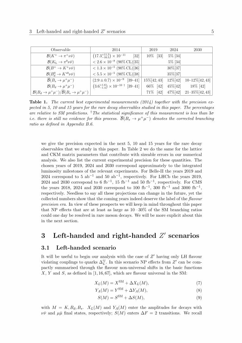
we give the precision expected in the next 5, 10 and 15 years for the rare decayobservables that we study in this paper. In Table 2 we do the same for the latticeand CKM matrix parameters that contribute with sizeable errors in our numericalanalysis. We also list the current experimental precision for these quantities. Thechosen years of 2019, 2024 and 2030 correspond approximately to the integratedluminosity milestones of the relevant experiments. For Belle-II the years 2019 and2024 correspond to 5 ab−1 and 50 ab−1, respectively. For LHCb the years 2019,2024 and 2030 correspond to 6 fb−1, 15 fb−1 and 50 fb−1, respectively. For CMSthe years 2018, 2024 and 2030 correspond to 100 fb−1, 300 fb−1 and 3000 fb−1,respectively. Needless to say all these projections can change in the future, yet thecollected numbers show that the coming years indeed deserve the label of the flavourprecision era. In view of these prospects we will keep in mind throughout this paperthat NP effects that are at least as large as 10 – 30% of the SM branching ratioscould one day be resolved in rare meson decays. We will be more explicit about thisin the next section.
3 Left-handed and right-handed Z ′ scenarios
3.1 Left-handed scenario
It will be useful to begin our analysis with the case of Z ′ having only LH flavourviolating couplings to quarks ∆ij
L . In this scenario NP effects from Z ′ can be com-pactly summarised through the flavour non-universal shifts in the basic functionsX, Y and S, as defined in [1, 16,67], which are flavour universal in the SM:
XL(M) = XSM + ∆XL(M), (7)
YA(M) = Y SM + ∆YA(M), (8)
S(M) = SSM + ∆S(M), (9)
with M = K,Bd, Bs. XL(M) and YA(M) enter the amplitudes for decays withνν̄ and µµ̄ final states, respectively; S(M) enters ∆F = 2 transitions. We recall
3 Left-handed and right-handed Z ′ scenarios 6
2014 2019 2024 2030
FBs (227.7± 4.5) MeV [44] < 1% [45]
FBd(190.5± 4.2) MeV [44] < 1% [45]
FBs
√B̂Bs (266± 18) MeV [44] 2.5% [45] < 1% [46]
FBd
√B̂Bd
(216± 15) MeV [44] 2.5% [45] < 1% [46]
B̂K 0.766± 0.010 [44] < 1% [45]
|Vub|incl (4.40± 0.25)× 10−3[44] 5% [37] 3% [37]
|Vub|excl (3.42± 0.31)× 10−3[44] 12% †† [37] 5% †† [37]
|Vcb|incl (42.4± 0.9)× 10−3 [47] 1% [48] < 1% [48]
|Vcb|excl (39.4± 0.6)× 10−3 [44] 1% [48] < 1% [48]
γ (70.1± 7.1)◦ † [49] 6% [37] 1.5% [37] 1.3%[43]
φSMd = 2β (43.0+1.6
−1.4)◦ [50] ∼ 1◦ ‡[51, 52]
φSMs = −2βs (0± 4)◦ [50] 1.4◦ [43] ∼ 1◦ ‡[53]
Table 2. Current best determinations and future forecasts for the precision of lattice and CKMmatrix parameters that contribute with sizeable errors in our numerical analysis. †Combinedfit from charmed B decay modes. ††These predictions assume dominant lattice errors. ‡At thisprecision the theoretical uncertainty due to penguin pollution in the dominant decay modes usedto extract these phases starts to dominate.
that the functions XSM, Y SM and SSM enter the top quark contributions to thecorresponding amplitudes in the SM. We suppressed here for simplicity the functionsrelated to vector (V ) couplings. We will return to them later on.
In what follows we will concentrate our discussion mainly on the functions∆XL(M), since in the left-handed scenario (LHS) ∆YA(M) are given by [16]
∆YA(K) = ∆XL(K)∆µµ̄A
∆νν̄L
, ∆YA(Bq) = ∆XL(Bq)∆µµ̄A
∆νν̄L
, (10)
as follows from the definitions of these functions given in Appendix A.The fundamental equations for the next steps of our analysis are the correlations
in the LHS between ∆X(M) and ∆S(M) derived in [16]. Rewriting them in a formsuitable for our applications we find
∆XL(K)√∆S(K)
=∆XL(Bq)√
∆S(Bq)∗=
∆νν̄L
2MZ′gSM
√r̃
= 0.25
[∆νν̄L
3.0
] [15 TeV
MZ′
], (11)
where r̃ is a QCD correction which depends on the Z ′ mass [16] (r̃ ≈ 0.90 forMZ′ = 50 TeV, but its dependence on MZ′ is very weak), and
g2SM = 4
M2WG
2F
2π2= 1.78137× 10⁻⁷ GeV−2 , (12)
where GF is the Fermi constant.Now comes an important observation: in the limit where the Z ′ coupling ∆sd
L
is approximately real and the εK constraint is easily satisfied, the allowed rangefor ∆S(K) can be much larger than the ones for ∆S(Bq) even if the ratios in (11)
3 Left-handed and right-handed Z ′ scenarios 7
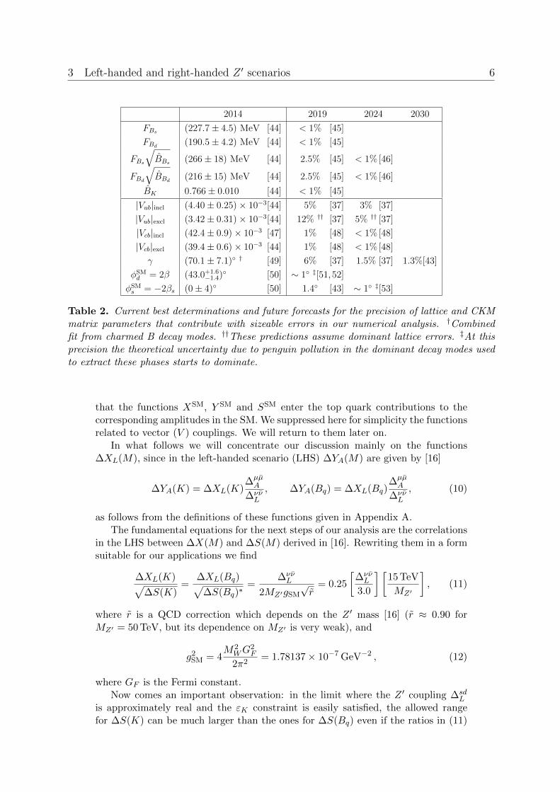
|εK | = 2.228(11)× 10−3 [54] αs(MZ) = 0.1185(6) [55]
∆MK = 0.5292(9)× 10−2 ps−1[54] ms(2 GeV) = 93.8(24) MeV [44]
∆Md = 0.507(4) ps−1 [56] mc(mc) = 1.279(13) GeV [57]
∆Ms = 17.72(4) ps−1 [56] mb(mb) = 4.19+0.18−0.06 GeV [54]
|Vus| = 0.2252(9) [56] mt(mt) = 163(1) GeV [58,59]
∆Γs/Γs = 0.123(17) [56] FK = 156.1(11) MeV [58]
mK = 497.614(24) MeV [54] FB+ = 185(3) MeV [60]
mBd= mB+ = 5279.2(2) MeV [55] κε = 0.94(2) [61,62]
mBs = 5366.8(2) MeV [55] ηcc = 1.87(76) [63]
τB± = 1.642(8) ps [56] ηtt = 0.5765(65) [64]
τBd= 1.519(7) ps [56] ηct = 0.496(47) [65]
τBs = 1.509(11) ps [56] ηB = 0.55(1) [64,66]
Table 3. Values of other experimental and theoretical quantities used as input parameters. Forfuture updates see PDG [55], FLAG [44] and HFAG [56].
are flavour universal. Indeed the ∆S(Bq) are directly constrained by the B0q − B̄0
q
mass differences ∆Mq because the function SSM enters the top quark contribution to∆Mq, which is by far dominant in the SM. On the other hand ∆MK is dominated inthe SM by charm quark contribution and the function S is multiplied there by smallCKM factors. Consequently, the shift ∆S(K) is allowed to be much larger than theshifts in ∆S(Bq), with interesting consequences for rareK decays as discussed below.Of course this assumes that the SM gives a good description of the experimentalvalues of εK and ε′/ε. We will relax this assumption later.
Let us first illustrate the case of ∆S(Bs) in the simplified scenario where ∆bsL is
real, in accordance with the small CP violation observed in the Bs system. Assumingthen that a NP contribution to ∆Ms at the level of 15% is still allowed, the resultof taking into account all the experimental and hadronic uncertainties implies thatonly |∆S(Bs)| ≤ 0.36 is allowed by present data. This gives
|∆XL(Bq)| ≤ 0.16
√|∆S(Bq)|
0.36
[∆νν̄L
3.0
] [15 TeV
MZ′
]. (13)
Since XSM ≈ 1.46, the shift |∆XL(Bq)| = 0.16 amounts to about 11% at thelevel of the amplitude and 22% for the branching ratios. Such NP effects could inprinciple one day be measured in b→ sνν̄ transitions such as Bd → K(K∗)νν̄ andB → Xsνν̄, and can still be increased by increasing slightly ∆νν̄
L or lowering MZ′ .However, this analysis shows that with the help of a Z ′ with only LH couplings onecannot reach the Zeptouniverse using Bs decays, although distance scales in theballpark of 10−20m, corresponding to 15 TeV, could be resolved. A similar analysiscan be performed for the function YA(Bs) relevant for Bs → µ+µ−: as Y SM ≈ 0.96,a shift of |∆YA(Bs)| = 0.16 results in a 33% modification in the branching ratio.
For Bd the discussion is complicated by the significant phase of Vtd. Because|Vtd| ≈ 0.25|Vts|, at first sight one may expect the shortest distance scales that canbe resolved with rare Bd decays to be about two times higher than the ones forBs. But, as seen in (11) for fixed lepton couplings, only MZ′ and the ∆F = 2constraints on S determine the maximal size of ∆F = 1 effects, independently ofthe CKM matrix elements. Similar effects to the ones allowed for rare Bs decays
3 Left-handed and right-handed Z ′ scenarios 8
-0.2 -0.1 0.0 0.1 0.2- Π
2
- Π
4
0
Π
4
Π
2
DLbs
ΦLbs
-0.15 -0.10 -0.05 0.00 0.05 0.10 0.15- Π
2
- Π
4
0
Π
4
Π
2
DLbd
ΦLbd
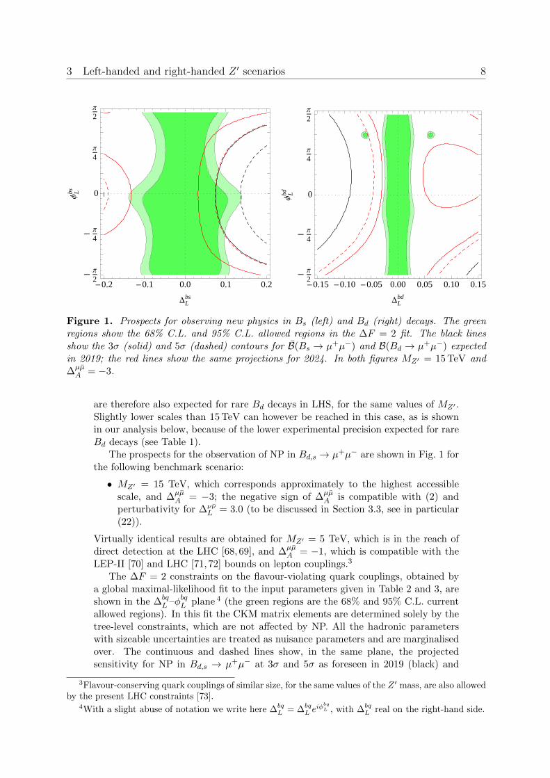
Figure 1. Prospects for observing new physics in Bs (left) and Bd (right) decays. The greenregions show the 68% C.L. and 95% C.L. allowed regions in the ∆F = 2 fit. The black linesshow the 3σ (solid) and 5σ (dashed) contours for B̄(Bs → µ+µ−) and B(Bd → µ+µ−) expectedin 2019; the red lines show the same projections for 2024. In both figures MZ′ = 15 TeV and∆µµ̄A = −3.
are therefore also expected for rare Bd decays in LHS, for the same values of MZ′ .Slightly lower scales than 15 TeV can however be reached in this case, as is shownin our analysis below, because of the lower experimental precision expected for rareBd decays (see Table 1).
The prospects for the observation of NP in Bd,s → µ+µ− are shown in Fig. 1 forthe following benchmark scenario:
• MZ′ = 15 TeV, which corresponds approximately to the highest accessiblescale, and ∆µµ̄
A = −3; the negative sign of ∆µµ̄A is compatible with (2) and
perturbativity for ∆νν̄L = 3.0 (to be discussed in Section 3.3, see in particular
(22)).
Virtually identical results are obtained for MZ′ = 5 TeV, which is in the reach ofdirect detection at the LHC [68, 69], and ∆µµ̄
A = −1, which is compatible with theLEP-II [70] and LHC [71,72] bounds on lepton couplings.3
The ∆F = 2 constraints on the flavour-violating quark couplings, obtained bya global maximal-likelihood fit to the input parameters given in Table 2 and 3, areshown in the ∆bq
L –φbqL plane 4 (the green regions are the 68% and 95% C.L. currentallowed regions). In this fit the CKM matrix elements are determined solely by thetree-level constraints, which are not affected by NP. All the hadronic parameterswith sizeable uncertainties are treated as nuisance parameters and are marginalisedover. The continuous and dashed lines show, in the same plane, the projectedsensitivity for NP in Bd,s → µ+µ− at 3σ and 5σ as foreseen in 2019 (black) and
3Flavour-conserving quark couplings of similar size, for the same values of the Z ′ mass, are also allowedby the present LHC constraints [73].
4With a slight abuse of notation we write here ∆bqL = ∆bq
L eiφbq
L , with ∆bqL real on the right-hand side.
3 Left-handed and right-handed Z ′ scenarios 9
2024 (red), using the estimates of Table 1. In all these projections we assume nodeviations in the ∆F = 2 observables in order to give the most optimistic predictionfor the sensitivity of rare decays. We therefore use the future errors also for theCKM matrix elements and for the hadronic parameters, assuming SM-like centralvalues. The impact of this choice on the ∆F = 1 projections is however moderate.
These figures show that already in five years from now it could be possible toprobe scales of 15 TeV with rare Bs decays by observing deviations from the SMpredictions at the level of 3σ, and reaching a 5σ discovery with more data in thefollowing years. On the other hand, for Bd a 3σ effect can be achieved only withthe full sensitivity in about ten years from now, for the same value of MZ′ .
The corrections from NP to the Wilson coefficients C9 and C10, which weightthe semileptonic operators in the effective Hamiltonian relevant for b → sµ+µ−
transitions (see Appendix B.5) as used in the recent literature (see e.g. [17,19,74–78])are given as follows [16]
sin2 θWCNP9 = − 1
g2SMM
2Z′
∆sbL ∆µµ̄
V
V ∗tsVtb, (14)
sin2 θWCNP10 = − 1
g2SMM
2Z′
∆sbL ∆µµ̄
A
V ∗tsVtb= −∆YA(Bs), (15)
where CNP9 involves the leptonic vector coupling of Z ′ and CNP
10 the axial-vector one.CNP
9 plays a crucial role in Bd → K∗µ+µ− transitions, CNP10 for Bs → µ+µ tran-
sitions and both coefficients are relevant for Bd → Kµ+µ−. The SU(2)L relationbetween the leptonic couplings in (2) implies the following important relation [17]
− sin2 θWCNP9 = 2∆XL(Bs) + ∆YA(Bs) (16)
which leads to a triple correlation between b → sνν̄ transitions, Bs → µµ̄ and thecoefficient CNP
9 or equivalently Bd → K∗µ+µ−. Thus even if ∆νν̄L and ∆µµ̄
A areindependent of each other, once they are fixed the values of the coupling ∆µµ̄
V andof CNP
9 are known. We will use these relations in the next section.Our study of the K system is eased by the analysis in [31], where an upper
bound on the coupling ∆sdL from ∆MK has been derived, assuming conservatively
that the NP contribution is at most as large as the short distance SM contributionto ∆MK . Assuming that the NP contribution to ∆MK is at most 30% of its SMvalue, and rescaling the formula (70) in [31], we find the upper limit
|∆sdL | ≤ 0.1
[MZ′
100 TeV
], (17)
which is clearly in the perturbative regime, and is still the case for an MZ′ aslarge as 2000 TeV. With |Vtd| = 8.5 × 10⁻³ and |Vts| = 0.040 this corresponds to|∆S(K)| ≤ 137. Then, again from (11), one has, for real ∆sd
L ,
|∆XL(K)| ≤ 0.44
√|∆S(K)|
137
[∆νν̄L
3.0
] [100 TeV
MZ′
]. (18)
This shift for MZ′ in the ballpark of 100 TeV implies a correction of approximately50% to the branching ratio for K+ → π+νν̄ but no contribution to KL → π0νν̄ sincewe are assuming ∆sd
L to be real. This clearly shows a non-MFV structure of NP
3 Left-handed and right-handed Z ′ scenarios 10
-6 -4 -2 0 2 4 6- Π
2
- Π
4
0
Π
2
Π
2
DLsd � 103
ΦLsd
-0.06 -0.04 -0.02 0.00 0.02 0.04 0.06- Π
2
- Π
4
0
Π
4
Π
2
DLsd
ΦLsd
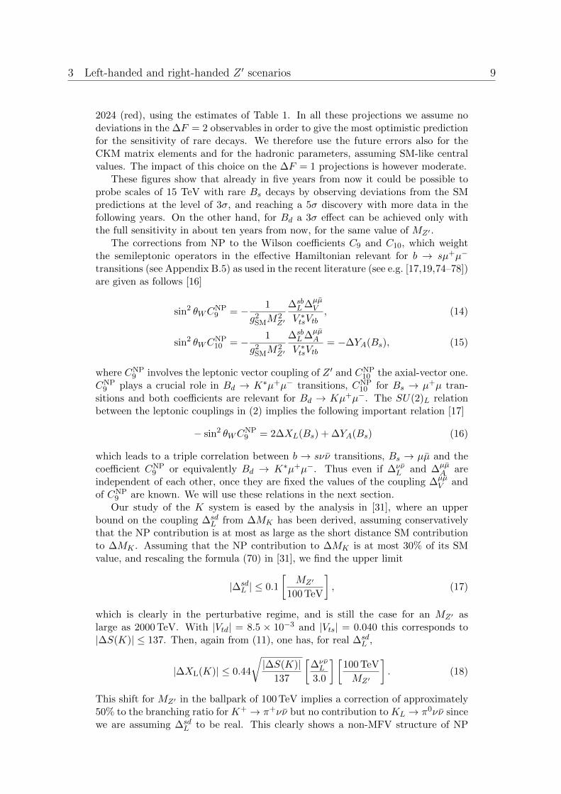
Figure 2. Prospects for observing new physics in K decays. The green regions show the 68%C.L. and 95% C.L. allowed regions in the ∆F = 2 fit. The contours show the 3σ and 5σ projec-tions for B(K+ → π+νν̄) in 2019 and 2024, the colours are as in Fig. 1. Left: MZ′ = 5 TeVand ∆νν̄
L = 1. Right: MZ′ = 50 TeV and ∆νν̄L = 3.
because in models with MFV the branching ratio for KL → π0νν̄ is automaticallymodified when the one for K+ → π+νν̄ is modified. If on the other hand ∆sd
L ismade complex, significant NP contributions to KL → π0νν̄ are in general subjectto severe constraints from εK and ε′/ε, unless ∆sd
L is purely imaginary, in whichcase the NP contributions to εK vanish and the effects in B(K+ → π+νν̄) andB(KL → π0νν̄) are correlated as in MFV. We will perform a more detailed analysisof these two decays and their correlation in Section 3.3. Let us discuss here justK+ → π+νν̄, as this decay will be the first to be measured precisely.
Fig. 2 shows the prospects for K+ → π+νν̄, together with the ∆S = 2 con-straints, in the ∆sd
L –φsdL plane. We show two different scenarios:
• a beyond-LHC scale of MZ′ = 50 TeV with ∆νν̄L = 3;
• an LHC scale of MZ′ = 5 TeV with ∆νν̄L = 1.
The conventions and colours are the same as in Fig. 1. Notice the strong boundfrom εK for large values of the phase φsdL , which implies that for NP at high scaleswith generic CP structure at most a 3σ effect can be expected with the precisionattainable at the end of the next decade. For real or imaginary couplings, on thecontrary, it is evident that scales of 50–100 TeV or even higher may be accessiblethrough K decays.
The overall message that emerges from the plots in Figs. 1 and 2 is that throughrare meson decays one can resolve energy scales beyond those directly accessible atthe LHC: at least in the LHS with suitable values of the Z ′ couplings one can stillexpect deviations from the SM at the level of 3 – 5σ with the experimental progressof the next few years that are consistent with perturbativity and the meson mixingconstraints, for MZ′ in the ranges described above.
We want to stress once more that the results discussed here correspond to the
3 Left-handed and right-handed Z ′ scenarios 11
most optimistic scenarios and to the largest couplings compatible with all consideredconstraints. Needless to say, in the case of smaller couplings, or in the presence ofsome approximate flavour symmetry, the scales that may eventually be accessiblethrough rare meson decays are much lower.
3.2 Right-handed scenario
If only RH couplings are present the results of the ∆F = 2 LHS analysis remainunchanged as the relevant hadronic matrix elements – calculated in lattice QCD– are insensitive to the sign of γ5. Therefore, as far as ∆F = 2 processes areconcerned, it is impossible to state whether in the presence of couplings of only onechirality the deviations from SM expectations are caused by LH or RH currents [16].In order to make this distinction one has to study ∆F = 1 processes. In particularin the right-handed scenario (RHS) the relations (10) are modified to
∆YA(K) = −∆XR(K)∆µµ̄A
∆νν̄L
, ∆YA(Bq) = −∆XR(Bq)∆µµ̄A
∆νν̄L
, (19)
where the sign flip plays a crucial role. The functions ∆XR(M) are obtained from∆XL(M) by replacing the LH quark couplings by the RH ones. We also find forthe coefficient of the primed operator C ′9
− sin2 θWC′9 = 2∆XR(Bs) + ∆YA(Bs). (20)
We refer to the Appendix A for explicit formulae for all the involved functions.Therefore the correlations between decays with νν̄ and µµ̄ in the final state
are different in LH and RH scenarios. In particular angular observables in Bd →K∗µ+µ− and also the decay Bd → Kµ+µ− can help in the distinction betweenLHS and RHS, as the presence of RH currents is signalled by the effects of primedoperators. In the future the correlation between the decays Bd → K∗νν̄ and Bd →Kνν̄ will be able by itself to identify RH currents at work [74,79–84]. We will showthis explicitly in the following sections.
3.3 Numerical analysis
We will now perform a numerical study of the ∆F = 1 effects that can be expectedfor MZ′ close to its maximal value, and of their correlations. As already indicatedby our preceding analysis, the ∆F = 2 constraints in these scenarios will not allowlarge Z ′ couplings to quarks, but the lepton couplings could be significantly largerthan the SM Z boson couplings, which read 5
∆νν̄L (Z) = −0.372, ∆µµ̄
A (Z) = 0.372, ∆µµ̄V (Z) = −0.028 . (21)
Working with MZ′ ≥ 15 TeV we will set
∆νν̄L = ±3.0, ∆µµ̄
A = ∓3.0, ∆µµ̄V = ±3.0 . (22)
where the signs are chosen in order to satisfy the SU(2)L relation (2) in the perturba-tivity regime. At MZ′ = 15 TeV, as well as for the higher masses considered below,
3 Left-handed and right-handed Z ′ scenarios 12
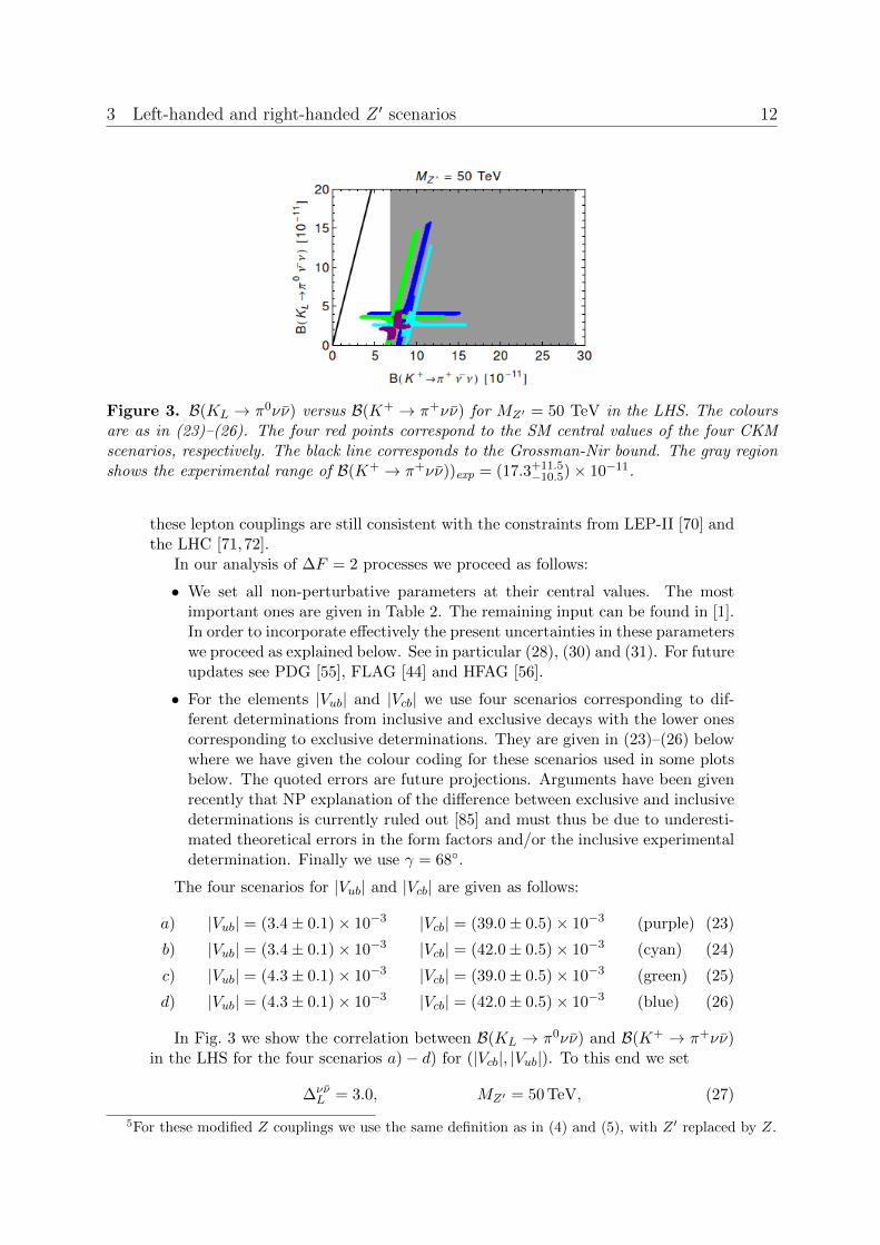
Figure 3. B(KL → π0νν̄) versus B(K+ → π+νν̄) for MZ′ = 50 TeV in the LHS. The coloursare as in (23)–(26). The four red points correspond to the SM central values of the four CKMscenarios, respectively. The black line corresponds to the Grossman-Nir bound. The gray regionshows the experimental range of B(K+ → π+νν̄))exp = (17.3+11.5
−10.5)× 10−11.
these lepton couplings are still consistent with the constraints from LEP-II [70] andthe LHC [71,72].
In our analysis of ∆F = 2 processes we proceed as follows:
• We set all non-perturbative parameters at their central values. The mostimportant ones are given in Table 2. The remaining input can be found in [1].In order to incorporate effectively the present uncertainties in these parameterswe proceed as explained below. See in particular (28), (30) and (31). For futureupdates see PDG [55], FLAG [44] and HFAG [56].
• For the elements |Vub| and |Vcb| we use four scenarios corresponding to dif-ferent determinations from inclusive and exclusive decays with the lower onescorresponding to exclusive determinations. They are given in (23)–(26) belowwhere we have given the colour coding for these scenarios used in some plotsbelow. The quoted errors are future projections. Arguments have been givenrecently that NP explanation of the difference between exclusive and inclusivedeterminations is currently ruled out [85] and must thus be due to underesti-mated theoretical errors in the form factors and/or the inclusive experimentaldetermination. Finally we use γ = 68◦.
The four scenarios for |Vub| and |Vcb| are given as follows:
a) |Vub| = (3.4± 0.1)× 10−3 |Vcb| = (39.0± 0.5)× 10−3 (purple) (23)
b) |Vub| = (3.4± 0.1)× 10−3 |Vcb| = (42.0± 0.5)× 10−3 (cyan) (24)
c) |Vub| = (4.3± 0.1)× 10−3 |Vcb| = (39.0± 0.5)× 10−3 (green) (25)
d) |Vub| = (4.3± 0.1)× 10−3 |Vcb| = (42.0± 0.5)× 10−3 (blue) (26)
In Fig. 3 we show the correlation between B(KL → π0νν̄) and B(K+ → π+νν̄)in the LHS for the four scenarios a)− d) for (|Vcb|, |Vub|). To this end we set
∆νν̄L = 3.0, MZ′ = 50 TeV, (27)
5For these modified Z couplings we use the same definition as in (4) and (5), with Z ′ replaced by Z.
3 Left-handed and right-handed Z ′ scenarios 13
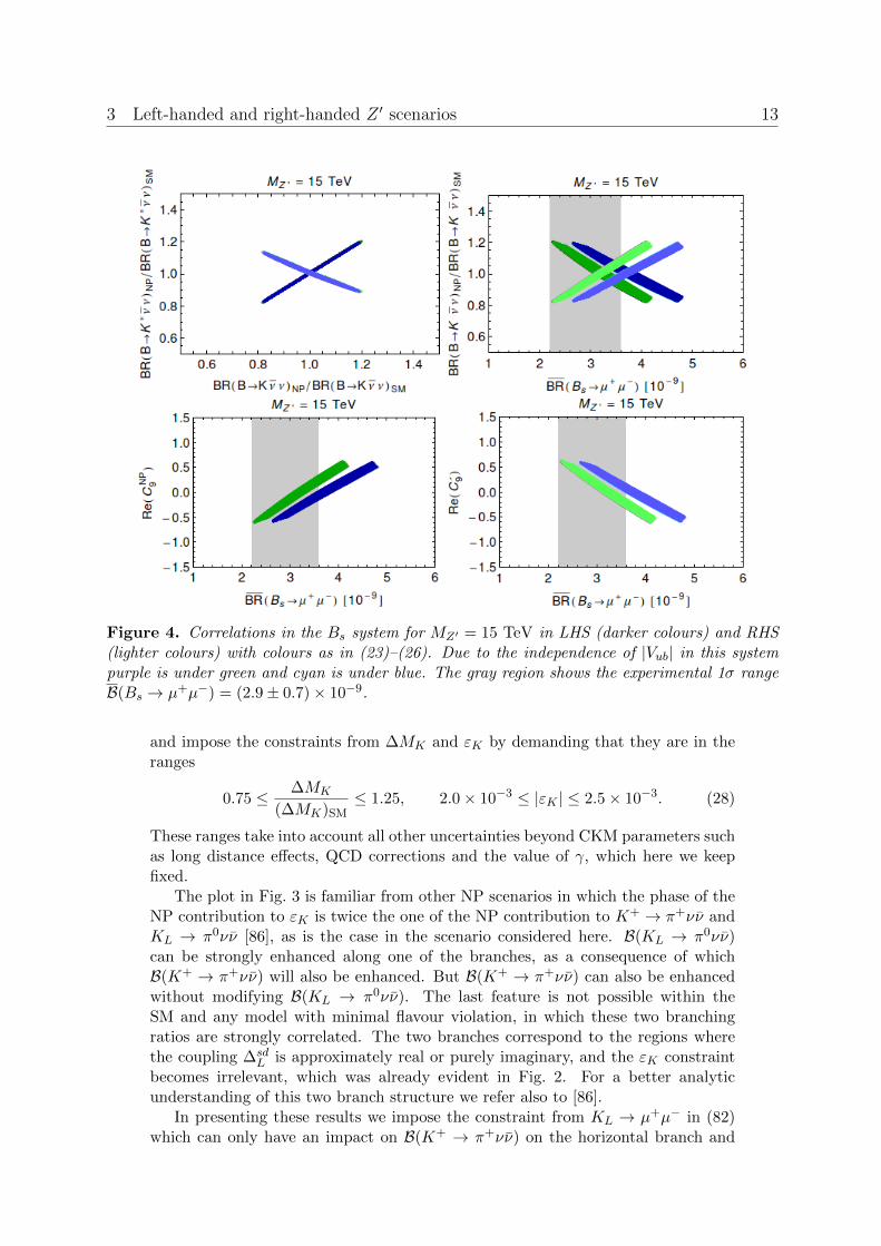
Figure 4. Correlations in the Bs system for MZ′ = 15 TeV in LHS (darker colours) and RHS(lighter colours) with colours as in (23)–(26). Due to the independence of |Vub| in this systempurple is under green and cyan is under blue. The gray region shows the experimental 1σ rangeB(Bs → µ+µ−) = (2.9± 0.7)× 10−9.
and impose the constraints from ∆MK and εK by demanding that they are in theranges
0.75 ≤ ∆MK
(∆MK)SM≤ 1.25, 2.0× 10⁻³ ≤ |εK | ≤ 2.5× 10⁻³. (28)
These ranges take into account all other uncertainties beyond CKM parameters suchas long distance effects, QCD corrections and the value of γ, which here we keepfixed.
The plot in Fig. 3 is familiar from other NP scenarios in which the phase of theNP contribution to εK is twice the one of the NP contribution to K+ → π+νν̄ andKL → π0νν̄ [86], as is the case in the scenario considered here. B(KL → π0νν̄)can be strongly enhanced along one of the branches, as a consequence of whichB(K+ → π+νν̄) will also be enhanced. But B(K+ → π+νν̄) can also be enhancedwithout modifying B(KL → π0νν̄). The last feature is not possible within theSM and any model with minimal flavour violation, in which these two branchingratios are strongly correlated. The two branches correspond to the regions wherethe coupling ∆sd
L is approximately real or purely imaginary, and the εK constraintbecomes irrelevant, which was already evident in Fig. 2. For a better analyticunderstanding of this two branch structure we refer also to [86].
In presenting these results we impose the constraint from KL → µ+µ− in (82)which can only have an impact on B(K+ → π+νν̄) on the horizontal branch and
3 Left-handed and right-handed Z ′ scenarios 14
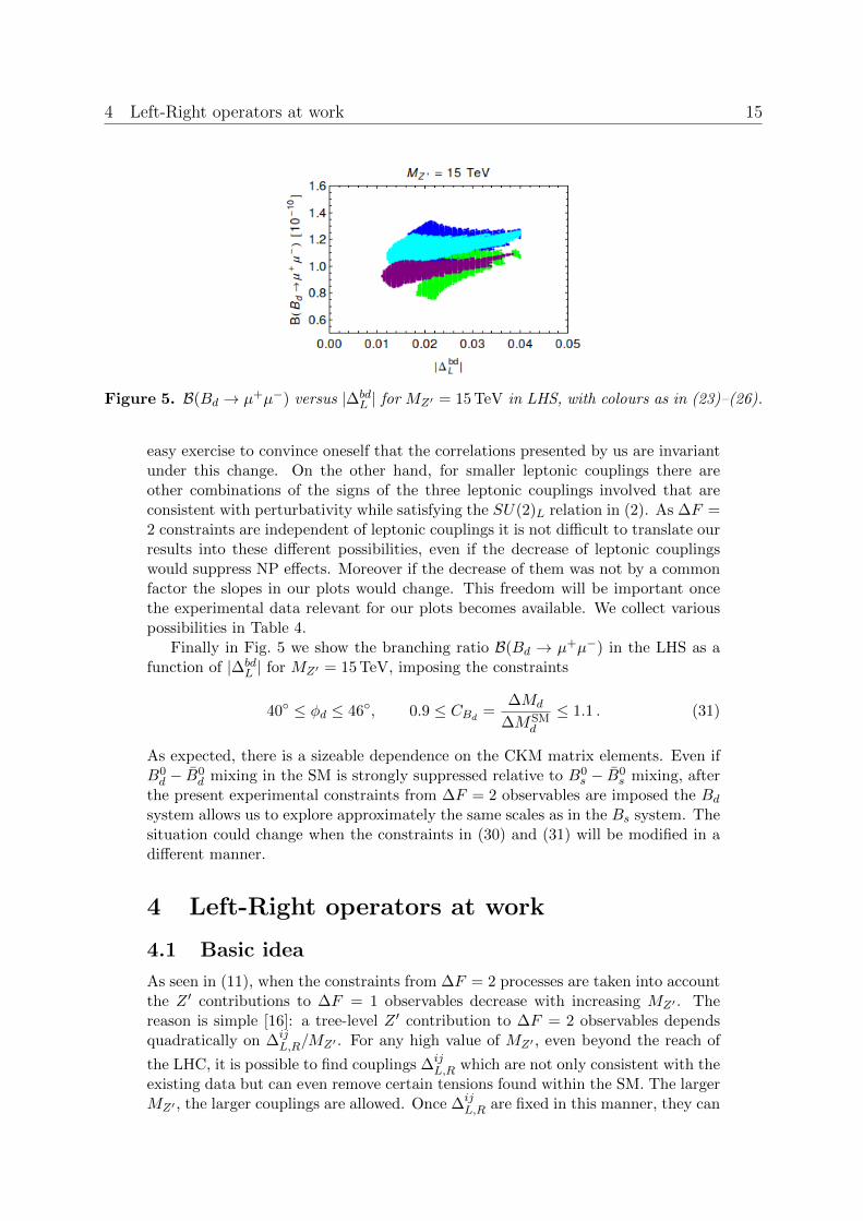
∆νν̄L ∆µµ̄
A ∆µµ̄A (1, 1) (1, 2) (2, 1) (2, 2)
+ + + +(−) +(−) − +
+ − + +(−) −(+) + −+ − − +(−) −(+) − +
Table 4. Correlations (+) and anti-correlations (−) between various observables for differentsigns of the couplings. (n,m) denotes the entry in the 2× 2 matrix in Fig. 4. For the elements(1, 1) and (1, 2) the signs correspond to LHS (RHS). Flipping simultaneously the signs of allcouplings does not change the correlations.
not on B(KL → π0νν̄). Because in this scenario the couplings ∆νν̄L and ∆µµ̄
A haveopposite signs, in the LHS B(K+ → π+νν̄) and B(KL → µ+µ−) are anti-correlatedso that the constraint in (82) has no impact on the upper bound on B(K+ → π+νν̄).On the other hand, for the chosen signs of leptonic couplings these two branchingratios are correlated in the RH scenario and the maximal values of B(K+ → π+νν̄)on the horizontal branch could in principle be smaller than the ones shown in Fig. 3due to the bound in (82). However, for the chosen parameters this turns out not tobe the case.
As far as the second branch is concerned, as recently analysed in [31] and knownfrom previous literature, the ratio ε′/ε can in principle have a large impact on thelargest allowed values of B(KL → π0νν̄) and B(K+ → π+νν̄) on the branch wherethese branching ratios are correlated. Unfortunately, the present large uncertaintiesin QCD penguin contributions to ε′/ε do not allow for firm conclusions and we donot show this constraint here.
We observe that large deviations from the SM can be measured even at suchhigh scales. Increasing MZ′ to 100 TeV would reduce NP effects by a factor of two,which could still be measured in the flavour precision era. We conclude thereforethat K+ → π+νν̄ and KL → π0νν̄ decays can probe the Zeptouniverse even if onlyLH or RH Z ′ couplings to quarks are present.
In Fig. 4 we show the correlations for decays sensitive to b → s transitions. Tothis end we set in accordance with the signs in (22)
∆νν̄L = 3.0, ∆µµ̄
A = −3.0, ∆µµ̄V = 3.0, MZ′ = 15 TeV . (29)
The ∆F = 2 constraint has been incorporated through the conditions
− 8◦ ≤ φs ≤ 8◦, 0.9 ≤ CBs ≡∆Ms
∆MSMs
≤ 1.1 (30)
As we have already shown, measurable NP effects are still present at 15 TeV providedthe lepton couplings are as large as assumed here, but for larger values of MZ′
the detection of NP would be hard. We consider therefore MZ′ = 15 TeV as anapproximate upper value in LHS and RHS that can still be probed in the flavourprecision era. It will be interesting to monitor the development of the values ofφs and CBs in the future. If they will depart significantly from their SM values,φs ≈ −2◦ and CBs = 1.0, NP effects could be observed in rare decays.
In presenting these results we have chosen the leptonic couplings in (29), but(22) admits a second possibility in which all the couplings are reversed. It is an
4 Left-Right operators at work 15
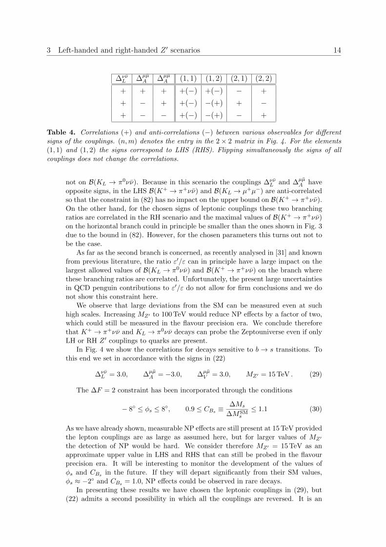
Figure 5. B(Bd → µ+µ−) versus |∆bdL | for MZ′ = 15 TeV in LHS, with colours as in (23)–(26).
easy exercise to convince oneself that the correlations presented by us are invariantunder this change. On the other hand, for smaller leptonic couplings there areother combinations of the signs of the three leptonic couplings involved that areconsistent with perturbativity while satisfying the SU(2)L relation in (2). As ∆F =2 constraints are independent of leptonic couplings it is not difficult to translate ourresults into these different possibilities, even if the decrease of leptonic couplingswould suppress NP effects. Moreover if the decrease of them was not by a commonfactor the slopes in our plots would change. This freedom will be important oncethe experimental data relevant for our plots becomes available. We collect variouspossibilities in Table 4.
Finally in Fig. 5 we show the branching ratio B(Bd → µ+µ−) in the LHS as afunction of |∆bd
L | for MZ′ = 15 TeV, imposing the constraints
40◦ ≤ φd ≤ 46◦, 0.9 ≤ CBd=
∆Md
∆MSMd
≤ 1.1 . (31)
As expected, there is a sizeable dependence on the CKM matrix elements. Even ifB0d − B̄0
d mixing in the SM is strongly suppressed relative to B0s − B̄0
s mixing, afterthe present experimental constraints from ∆F = 2 observables are imposed the Bdsystem allows us to explore approximately the same scales as in the Bs system. Thesituation could change when the constraints in (30) and (31) will be modified in adifferent manner.
4 Left-Right operators at work
4.1 Basic idea
As seen in (11), when the constraints from ∆F = 2 processes are taken into accountthe Z ′ contributions to ∆F = 1 observables decrease with increasing MZ′ . Thereason is simple [16]: a tree-level Z ′ contribution to ∆F = 2 observables dependsquadratically on ∆ij
L,R/MZ′ . For any high value of MZ′ , even beyond the reach of
the LHC, it is possible to find couplings ∆ijL,R which are not only consistent with the
existing data but can even remove certain tensions found within the SM. The largerMZ′ , the larger couplings are allowed. Once ∆ij
L,R are fixed in this manner, they can
4 Left-Right operators at work 16
be used to predict Z ′ effects in ∆F = 1 observables. However here NP contributionsto the amplitudes are proportional to ∆ij
L,R/M2Z′ and with the couplings proportional
to MZ′ , the Z ′ contributions to ∆F = 1 observables decrease with increasing MZ′ .But this stringent correlation is only present in the LHS and RHS considered
until now. If both couplings are present this correlation can be broken, simplybecause we then have four parameters instead of two in the Z ′ couplings to quarks ofeach meson system. As we will soon see, this will allow us to increase the resolutionof short distance scales and allow one to reach Zeptouniverse sensitivities also withthe help of Bs,d decays while satisfying their ∆F = 2 constraints.
4.2 L+R scenario
In the presence of both LH and RH couplings of a Z ′ gauge boson to SM quarksleft-right (LR) ∆F = 2 operators are generated whose contributions to the mixing
amplitudes M bq12 and M sd
12 in all three mesonic systems are enhanced through renor-malisation group effects relative to left-left (VLL) and right-right (VRR) operators.Moreover in the case of M sd
12 additional chiral enhancements of the hadronic matrixelements of LR operators are present. As pointed out in [31] this fact can be used tosuppress NP contributions to ∆MK through some fine-tuning between VLL, VRRand LR contributions, thereby allowing for larger contributions to K → ππ ampli-tudes while satisfying the ∆MK constraint in the limit of small NP phases. Here wegeneralise this idea to all three systems and NP phases in Z ′ contributions. Whilethe fine-tuning required in the case of K → ππ turned out to be rather large, it willbe more modest in the case at hand.6
To this end we write the Z ′ contributions to the mixing amplitudes as follows [16]:
(M∗12)sdZ′ =(∆sd
L )2
2M2Z′〈Q̂VLL
1 (MZ′)〉sdzsd, (32)
and
(M∗12)bqZ′ =(∆bq
L )2
2M2Z′〈Q̂VLL
1 (MZ′)〉bqzbq, (33)
where zsd and zbq are generally complex. We have
zsd =
[1 +
(∆sdR
∆sdL
)2
+ 2κsd∆sdR
∆sdL
], κsd =
〈Q̂LR1 (MZ′)〉sd
〈Q̂VLL1 (MZ′)〉sd
(34)
with an analogous expressions for zbq.Here using the technology of [87, 88] we have expressed zsd in terms of the
renormalisation scheme independent matrix elements
〈Q̂VLL1 (MZ′)〉sd = 〈QVLL
1 (MZ′)〉sd(
1 +11
3
αs(MZ′)
4π
), (35)
〈Q̂LR1 (MZ′)〉sd = 〈QLR
1 (MZ′)〉sd(
1− 1
6
αs(MZ′)
4π
)− αs(MZ′)
4π〈QLR
2 (MZ′)〉sd . (36)
6In order to distinguish this more general scenario from the LRS and ALRS in [16], where the LH andRH couplings were either equal or differed by sign, we denote it simply by L+R.
4 Left-Right operators at work 17
MZ′ 5 TeV 10 TeV 20 TeV 50 TeV 100 TeV 200 TeV
〈Q̂VLL1 (MZ′)〉sd 0.00158 0.00156 0.00153 0.00150 0.00148 0.00146
〈Q̂LR1 (MZ′)〉sd −0.183 −0.197 −0.211 −0.230 −0.244 −0.259
κsd(MZ′) −115.46 −126.51 −137.84 −153.24 −165.20 −177.41
〈Q̂VLL1 (MZ′)〉bd 0.0423 0.0416 0.0409 0.0401 0.0395 0.0390
〈Q̂LR1 (MZ′)〉bd −0.183 −0.195 −0.206 −0.222 −0.234 −0.246
κbd(MZ′) −4.33 −4.68 −5.04 −5.53 −5.92 −6.30
〈Q̂VLL1 (MZ′)〉bs 0.0622 0.0611 0.0601 0.0589 0.0581 0.0573
〈Q̂LR1 (MZ′)〉bs −0.268 −0.284 −0.301 −0.323 −0.340 −0.357
κbs(MZ′) −4.31 −4.66 −5.01 −5.48 −5.85 −6.23
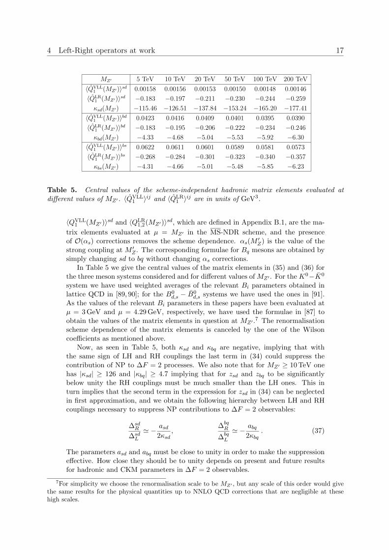
Table 5. Central values of the scheme-independent hadronic matrix elements evaluated atdifferent values of MZ′. 〈Q̂VLL
1 〉ij and 〈Q̂LR1 〉ij are in units of GeV3.
〈QVLL1 (MZ′)〉sd and 〈QLR
1,2(MZ′)〉sd, which are defined in Appendix B.1, are the ma-
trix elements evaluated at µ = MZ′ in the MS-NDR scheme, and the presenceof O(αs) corrections removes the scheme dependence. αs(M
′Z) is the value of the
strong coupling at M ′Z . The corresponding formulae for Bq mesons are obtained bysimply changing sd to bq without changing αs corrections.
In Table 5 we give the central values of the matrix elements in (35) and (36) forthe three meson systems considered and for different values of MZ′ . For the K0−K̄0
system we have used weighted averages of the relevant Bi parameters obtained inlattice QCD in [89, 90]; for the B0
d,s − B̄0d,s systems we have used the ones in [91].
As the values of the relevant Bi parameters in these papers have been evaluated atµ = 3 GeV and µ = 4.29 GeV, respectively, we have used the formulae in [87] toobtain the values of the matrix elements in question at MZ′ .
7 The renormalisationscheme dependence of the matrix elements is canceled by the one of the Wilsoncoefficients as mentioned above.
Now, as seen in Table 5, both κsd and κbq are negative, implying that withthe same sign of LH and RH couplings the last term in (34) could suppress thecontribution of NP to ∆F = 2 processes. We also note that for MZ′ ≥ 10 TeV onehas |κsd| ≥ 126 and |κbq| ≥ 4.7 implying that for zsd and zbq to be significantlybelow unity the RH couplings must be much smaller than the LH ones. This inturn implies that the second term in the expression for zsd in (34) can be neglectedin first approximation, and we obtain the following hierarchy between LH and RHcouplings necessary to suppress NP contributions to ∆F = 2 observables:
∆sdR
∆sdL
' − asd2κsd
,∆bqR
∆bqL
' −abq2κbq
. (37)
The parameters asd and abq must be close to unity in order to make the suppressioneffective. How close they should be to unity depends on present and future resultsfor hadronic and CKM parameters in ∆F = 2 observables.
7For simplicity we choose the renormalisation scale to be MZ′ , but any scale of this order would givethe same results for the physical quantities up to NNLO QCD corrections that are negligible at thesehigh scales.
4 Left-Right operators at work 18
0 500 1000 1500 200010-5
10-4
10-3
10-2
MZ' @TeVD
∆a s
d
50 100 150 20010-3
10-2
10-1
MZ' @TeVD
∆a b
s
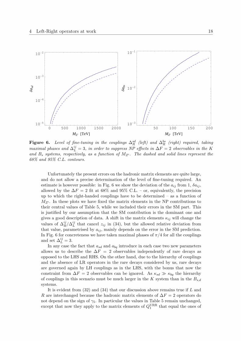
Figure 6. Level of fine-tuning in the couplings ∆sdR (left) and ∆bs
R (right) required, taking
maximal phases and ∆ijL = 3, in order to suppress NP effects in ∆F = 2 observables in the K
and Bs systems, respectively, as a function of MZ′. The dashed and solid lines represent the68% and 95% C.L. contours.
Unfortunately the present errors on the hadronic matrix elements are quite large,and do not allow a precise determination of the level of fine-tuning required. Anestimate is however possible: in Fig. 6 we show the deviation of the aij from 1, δaij ,allowed by the ∆F = 2 fit at 68% and 95% C.L. – or, equivalently, the precisionup to which the right-handed couplings have to be determined – as a function ofMZ′ . In these plots we have fixed the matrix elements in the NP contributions totheir central values of Table 5, while we included their errors in the SM part. Thisis justified by our assumption that the SM contribution is the dominant one andgives a good description of data. A shift in the matrix elements κij will change the
values of ∆ijR/∆
ijL that cancel zij in (34), but the allowed relative deviation from
that value, parametrised by aij , mainly depends on the error in the SM prediction.In Fig. 6 for concreteness we have taken maximal phases of π/4 for all the couplingsand set ∆ij
L = 3.In any case the fact that asd and abq introduce in each case two new parameters
allows us to describe the ∆F = 2 observables independently of rare decays asopposed to the LHS and RHS. On the other hand, due to the hierarchy of couplingsand the absence of LR operators in the rare decays considered by us, rare decaysare governed again by LH couplings as in the LHS, with the bonus that now theconstraint from ∆F = 2 observables can be ignored. As κsd � κbq the hierarchyof couplings in this scenario must be much larger in the K system than in the Bs,dsystems.
It is evident from (32) and (34) that our discussion above remains true if L andR are interchanged because the hadronic matrix elements of ∆F = 2 operators donot depend on the sign of γ5. In particular the values in Table 5 remain unchanged,except that now they apply to the matrix elements of QVRR
1 that equal the ones of
4 Left-Right operators at work 19
QVLL1 . In turn L and R are interchanged in (37) and consequently rare decays are
governed by RH couplings in this case. While these two opposite hierarchies cannotbe distinguished through ∆F = 2 observables they can be distinguished throughrare decays as we will demonstrate below.
This picture of short distances should be contrasted with the LR and ALRscenarios analysed in [16–19, 92–95], in which the LH and RH couplings were ofthe same size. In that case the LR operators dominate NP contributions to ∆F =2 observables, which implies significantly smaller allowed couplings, and in turnstronger constraints on the ∆F = 1 observables. Even if also there the signals fromLH or RH currents could in principle be observed in rare K and Bsd decays, theireffects will only be measurable for scales below 10 TeV.
The main message of this section is the following one: by appropriately choosingthe hierarchy between LH and RH flavour violating Z ′ couplings to quarks one caneliminate to a large extent the constraints from ∆F = 2 transitions even in thepresence of large CP-violating phases, and in this manner increase the resolution ofshort distance scales, which now would be probed solely by rare K and Bs,d decays.While in the Bd,s systems this can be done at the price of a mild fine-tuning, andallows one to reach the Zeptouniverse, in the K system it requires a fine-tuningof the couplings at the level of 1% – 1h because of the strong εK constraint (seeFig. 6). Notice however that K decays already allowed us to reach 100 TeV in theLHS without the need of right-handed couplings.
The implications of this are rather profound. Even if in the future SM wouldagree perfectly with all ∆F = 2 observables, this would not necessarily imply thatno NP effects can be seen in rare decays, even if the Z ′ is very heavy. The maximalvalue of the Z ′ mass, Mmax
Z′ , for which measurable effects in rare decays could inprinciple still be found, and perturbativity of couplings is respected, is again ratherdifferent in different systems, and depends on the assumed perturbativity upperbounds on Z ′ couplings and on the sensitivity of future experiments.
In Appendix B we give expressions for the rare decay branching ratio observ-ables B given in Table 1, which depend on the functions XL,R and YL,R listed inAppendix A. Combining these formulae gives the following relation for a non-zero∆XL(M) (as defined in (9))
MmaxZ′ = K(M)
√∣∣∣∣∆νν̄L
3.0
∣∣∣∣√√√√∣∣∣∣∣∆ij
L
3.0
∣∣∣∣∣√∣∣∣∣ 10%
δexp(M)
∣∣∣∣, (38)
where ij = sd, db, sb for M = K,Bd, Bs, respectively, and δexp(M) ≡ δB/B is theexperimental sensitivity that can be reached in M decays, as listed in Table 1. Forthe present CKM parameters the factors K(M) are as follows:
K(K) ≈ 1400 TeV, K(Bd) ≈ 280 TeV, K(Bs) ≈ 140 TeV. (39)
One has similar formulae for YA(M), but as Y SM ≈ 0.65XSM one can reach slightlyhigher values of MZ′ for the same experimental sensitivity. We note that this timethere is a difference between the Bd and Bs system, which was not the case inSection 3. We also note that, although these maximal values depend on the assumedmaximal values of the Z ′ couplings to SM fermions and the assumed sensitivity toNP, this is not a strong dependence due to the square roots involved. Using the
4 Left-Right operators at work 20
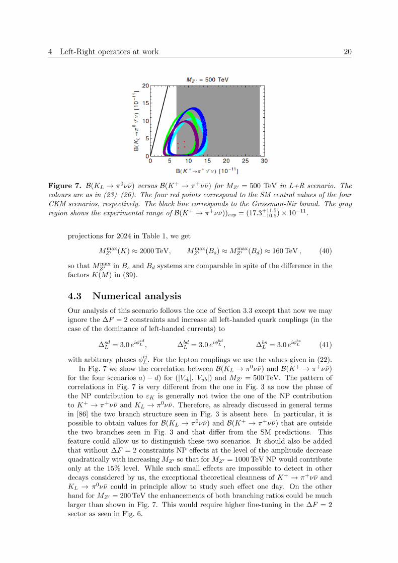
Figure 7. B(KL → π0νν̄) versus B(K+ → π+νν̄) for MZ′ = 500 TeV in L+R scenario. Thecolours are as in (23)–(26). The four red points correspond to the SM central values of the fourCKM scenarios, respectively. The black line corresponds to the Grossman-Nir bound. The grayregion shows the experimental range of B(K+ → π+νν̄))exp = (17.3+11.5
−10.5)× 10−11.
projections for 2024 in Table 1, we get
MmaxZ′ (K) ≈ 2000 TeV, Mmax
Z′ (Bs) ≈MmaxZ′ (Bd) ≈ 160 TeV , (40)
so that MmaxZ′ in Bs and Bd systems are comparable in spite of the difference in the
factors K(M) in (39).
4.3 Numerical analysis
Our analysis of this scenario follows the one of Section 3.3 except that now we mayignore the ∆F = 2 constraints and increase all left-handed quark couplings (in thecase of the dominance of left-handed currents) to
∆sdL = 3.0 eiφ
sdL , ∆bd
L = 3.0 eiφbdL , ∆bs
L = 3.0 eiφbsL (41)
with arbitrary phases φijL . For the lepton couplings we use the values given in (22).In Fig. 7 we show the correlation between B(KL → π0νν̄) and B(K+ → π+νν̄)
for the four scenarios a) − d) for (|Vcb|, |Vub|) and MZ′ = 500 TeV. The pattern ofcorrelations in Fig. 7 is very different from the one in Fig. 3 as now the phase ofthe NP contribution to εK is generally not twice the one of the NP contributionto K+ → π+νν̄ and KL → π0νν̄. Therefore, as already discussed in general termsin [86] the two branch structure seen in Fig. 3 is absent here. In particular, it ispossible to obtain values for B(KL → π0νν̄) and B(K+ → π+νν̄) that are outsidethe two branches seen in Fig. 3 and that differ from the SM predictions. Thisfeature could allow us to distinguish these two scenarios. It should also be addedthat without ∆F = 2 constraints NP effects at the level of the amplitude decreasequadratically with increasing MZ′ so that for MZ′ = 1000 TeV NP would contributeonly at the 15% level. While such small effects are impossible to detect in otherdecays considered by us, the exceptional theoretical cleanness of K+ → π+νν̄ andKL → π0νν̄ could in principle allow to study such effect one day. On the otherhand for MZ′ = 200 TeV the enhancements of both branching ratios could be muchlarger than shown in Fig. 7. This would require higher fine-tuning in the ∆F = 2sector as seen in Fig. 6.
4 Left-Right operators at work 21
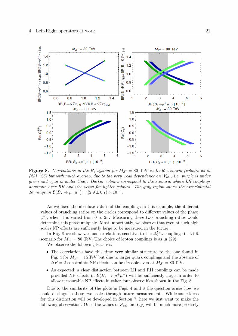
Figure 8. Correlations in the Bs system for MZ′ = 80 TeV in L+R scenario (colours as in(23)–(26) but with much overlap, due to the very weak dependence on |Vub|, i.e. purple is undergreen and cyan is under blue). Darker colours correspond to the scenario where LH couplingsdominate over RH and vice versa for lighter colours. The gray region shows the experimental1σ range in B(Bs → µ+µ−) = (2.9± 0.7)× 10−9.
As we fixed the absolute values of the couplings in this example, the differentvalues of branching ratios on the circles correspond to different values of the phaseφsdL , when it is varied from 0 to 2π. Measuring these two branching ratios woulddetermine this phase uniquely. Most importantly, we observe that even at such highscales NP effects are sufficiently large to be measured in the future.
In Fig. 8 we show various correlations sensitive to the ∆bsL,R couplings in L+R
scenario for MZ′ = 80 TeV. The choice of lepton couplings is as in (29).We observe the following features:
• The correlations have this time very similar structure to the one found inFig. 4 for MZ′ = 15 TeV but due to larger quark couplings and the absence of∆F = 2 constraints NP effects can be sizeable even at MZ′ = 80 TeV.
• As expected, a clear distinction between LH and RH couplings can be madeprovided NP effects in B(Bs → µ+µ−) will be sufficiently large in order toallow measurable NP effects in other four observables shown in the Fig. 8.
Due to the similarity of the plots in Figs. 4 and 8 the question arises how wecould distinguish these two scales through future measurements. While some ideasfor this distinction will be developed in Section 7, here we just want to make thefollowing observation. Once the values of Sψφ and CBs will be much more precisely
5 The case of a neutral scalar or pseudoscalar 22
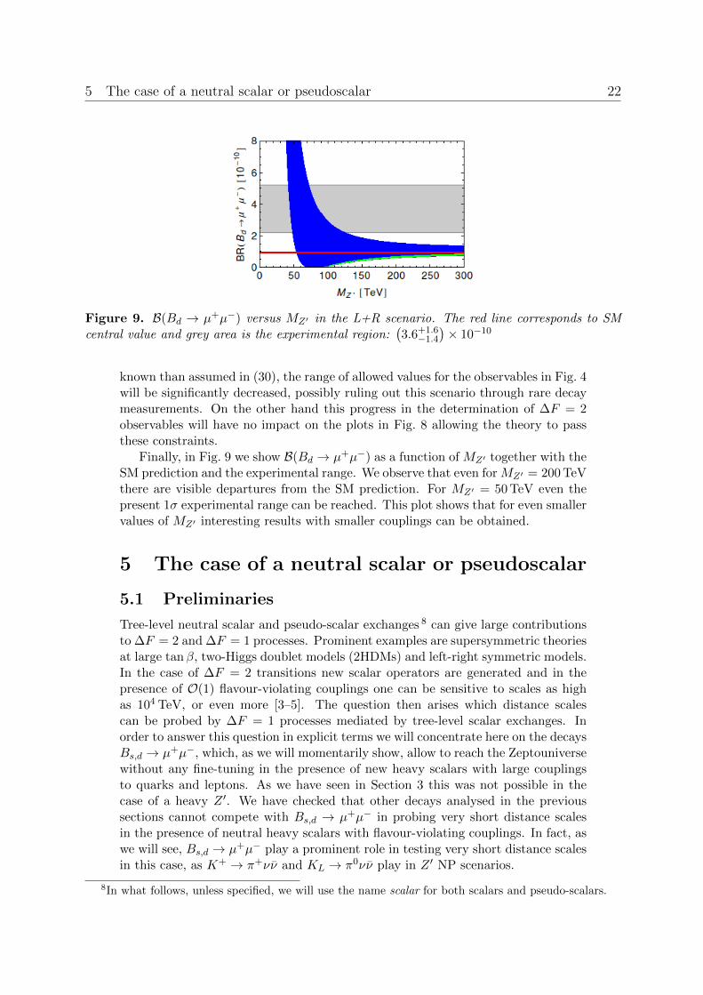
Figure 9. B(Bd → µ+µ−) versus MZ′ in the L+R scenario. The red line corresponds to SMcentral value and grey area is the experimental region:
(3.6+1.6−1.4
)× 10−10
known than assumed in (30), the range of allowed values for the observables in Fig. 4will be significantly decreased, possibly ruling out this scenario through rare decaymeasurements. On the other hand this progress in the determination of ∆F = 2observables will have no impact on the plots in Fig. 8 allowing the theory to passthese constraints.
Finally, in Fig. 9 we show B(Bd → µ+µ−) as a function of MZ′ together with theSM prediction and the experimental range. We observe that even for MZ′ = 200 TeVthere are visible departures from the SM prediction. For MZ′ = 50 TeV even thepresent 1σ experimental range can be reached. This plot shows that for even smallervalues of MZ′ interesting results with smaller couplings can be obtained.
5 The case of a neutral scalar or pseudoscalar
5.1 Preliminaries
Tree-level neutral scalar and pseudo-scalar exchanges 8 can give large contributionsto ∆F = 2 and ∆F = 1 processes. Prominent examples are supersymmetric theoriesat large tanβ, two-Higgs doublet models (2HDMs) and left-right symmetric models.In the case of ∆F = 2 transitions new scalar operators are generated and in thepresence of O(1) flavour-violating couplings one can be sensitive to scales as highas 104 TeV, or even more [3–5]. The question then arises which distance scalescan be probed by ∆F = 1 processes mediated by tree-level scalar exchanges. Inorder to answer this question in explicit terms we will concentrate here on the decaysBs,d → µ+µ−, which, as we will momentarily show, allow to reach the Zeptouniversewithout any fine-tuning in the presence of new heavy scalars with large couplingsto quarks and leptons. As we have seen in Section 3 this was not possible in thecase of a heavy Z ′. We have checked that other decays analysed in the previoussections cannot compete with Bs,d → µ+µ− in probing very short distance scalesin the presence of neutral heavy scalars with flavour-violating couplings. In fact, aswe will see, Bs,d → µ+µ− play a prominent role in testing very short distance scalesin this case, as K+ → π+νν̄ and KL → π0νν̄ play in Z ′ NP scenarios.
8In what follows, unless specified, we will use the name scalar for both scalars and pseudo-scalars.
5 The case of a neutral scalar or pseudoscalar 23
A very detailed analysis of generic scalar tree-level contributions to ∆F = 2and ∆F = 1 processes has been presented in [93, 94]. In particular in [94] generalformulae for various observables have been presented. We will not repeat theseformulae here but we will use them to derive a number of expressions that willallow us a direct comparison of this NP scenario with the Z ′ one.
Our goal then is to find out what is the highest energy scale which can beprobed by Bs,d → µ+µ− when the dominant NP contributions are tree-level scalarexchanges subject to present ∆F = 2 constraints and perturbativity. We will firstpresent general expressions and subsequently we will discuss in turn the cases anal-ogous to the Z ′ scenarios of Sections 3 and 4.
5.2 General formulae
Denoting by H a neutral scalar with mass MH the mixing amplitudes are given asfollows (q = s, d)
(M∗12)bqH = −
[(∆bq
L (H))2
2M2H
+(∆bq
R (H))2
2M2H
]〈Q̂SLL
1 (MH)〉bq−∆bqL (H)∆bq
R (H)
M2H
〈Q̂LR2 (MH)〉bq.
(42)
Here ∆bqL,R(H) are the left-handed and right-handed scalar couplings and the renor-
malisation scheme independent matrix elements are given as follows [88]
〈Q̂SLL1 (MH)〉bq = 〈QSLL
1 (MH)〉bq(
1 +9
2
αs(MH)
4π
)+
1
8
αs(MH)
4π〈QSLL
2 (MH)〉bq,
(43)
〈Q̂LR2 (MH)〉bq = 〈QLR
2 (MH)〉bq(
1− αs(MH)
4π
)− 3
2
αs(MH)
4π〈QLR
1 (MH)〉bq . (44)
The operators QSLL1,2 are defined in Appendix B.1. The operators QLR
1,2 were already
present in the case of Z ′ but now, as seen from (44), the operator QLR2 plays the
dominant role. In writing (42) we have used the fact that the matrix elements of theRH scalar operators QSRR
1,2 equal those of QSLL1,2 operators. The Wilson coefficients
of QSRR1,2 are represented in (42) by the term involving (∆bq
R (H))2.In analogy to (33) we can rewrite (42)
(M∗12)bqH = −(∆bq
L (H))2
2M2H
〈Q̂SLL1 (MH)〉bq z̃bq(MH), (45)
where z̃bq(MH) is generally complex, and is given by
z̃bq(MH) =
1 +
(∆bqR (H)
∆sdL (H)
)2
+ 2κ̃bq(MH)∆bqR (H)
∆bqL (H)
, (46)
κ̃bq(MH) =〈Q̂LR
2 (MH)〉sd
〈Q̂SLL1 (MH)〉sd
. (47)
In Table 6 we give the central values of the renormalization scheme independentmatrix elements of (43) and (44) for the three meson systems and for different valuesof MH , using the lattice results of [89–91] as in Table 5. For simplicity we set the
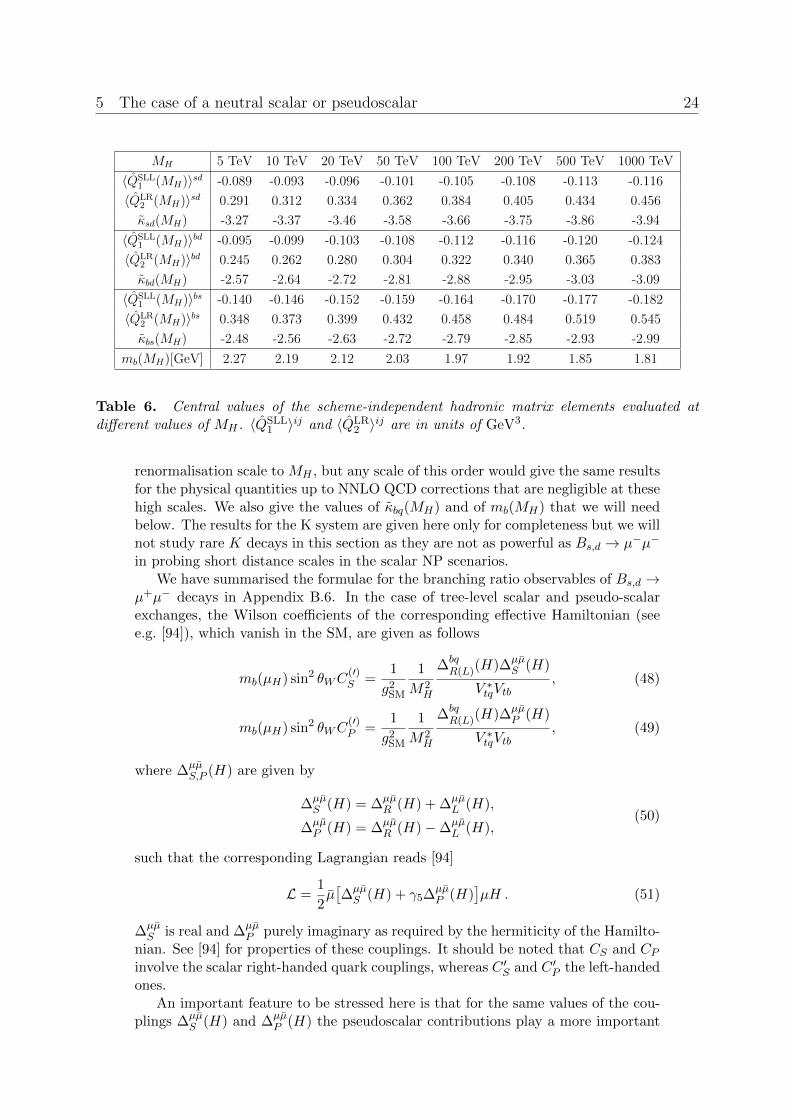
5 The case of a neutral scalar or pseudoscalar 24
MH 5 TeV 10 TeV 20 TeV 50 TeV 100 TeV 200 TeV 500 TeV 1000 TeV
〈Q̂SLL1 (MH)〉sd -0.089 -0.093 -0.096 -0.101 -0.105 -0.108 -0.113 -0.116
〈Q̂LR2 (MH)〉sd 0.291 0.312 0.334 0.362 0.384 0.405 0.434 0.456
κ̃sd(MH) -3.27 -3.37 -3.46 -3.58 -3.66 -3.75 -3.86 -3.94
〈Q̂SLL1 (MH)〉bd -0.095 -0.099 -0.103 -0.108 -0.112 -0.116 -0.120 -0.124
〈Q̂LR2 (MH)〉bd 0.245 0.262 0.280 0.304 0.322 0.340 0.365 0.383
κ̃bd(MH) -2.57 -2.64 -2.72 -2.81 -2.88 -2.95 -3.03 -3.09
〈Q̂SLL1 (MH)〉bs -0.140 -0.146 -0.152 -0.159 -0.164 -0.170 -0.177 -0.182
〈Q̂LR2 (MH)〉bs 0.348 0.373 0.399 0.432 0.458 0.484 0.519 0.545
κ̃bs(MH) -2.48 -2.56 -2.63 -2.72 -2.79 -2.85 -2.93 -2.99
mb(MH)[GeV] 2.27 2.19 2.12 2.03 1.97 1.92 1.85 1.81
Table 6. Central values of the scheme-independent hadronic matrix elements evaluated atdifferent values of MH . 〈Q̂SLL
1 〉ij and 〈Q̂LR2 〉ij are in units of GeV3.
renormalisation scale to MH , but any scale of this order would give the same resultsfor the physical quantities up to NNLO QCD corrections that are negligible at thesehigh scales. We also give the values of κ̃bq(MH) and of mb(MH) that we will needbelow. The results for the K system are given here only for completeness but we willnot study rare K decays in this section as they are not as powerful as Bs,d → µ−µ−
in probing short distance scales in the scalar NP scenarios.We have summarised the formulae for the branching ratio observables of Bs,d →
µ+µ− decays in Appendix B.6. In the case of tree-level scalar and pseudo-scalarexchanges, the Wilson coefficients of the corresponding effective Hamiltonian (seee.g. [94]), which vanish in the SM, are given as follows
mb(µH) sin2 θWC(′)S =
1
g2SM
1
M2H
∆bqR(L)(H)∆µµ̄
S (H)
V ∗tqVtb, (48)
mb(µH) sin2 θWC(′)P =
1
g2SM
1
M2H
∆bqR(L)(H)∆µµ̄
P (H)
V ∗tqVtb, (49)
where ∆µµ̄S,P (H) are given by
∆µµ̄S (H) = ∆µµ̄
R (H) + ∆µµ̄L (H),
∆µµ̄P (H) = ∆µµ̄
R (H)−∆µµ̄L (H),
(50)
such that the corresponding Lagrangian reads [94]
L =1
2µ̄[∆µµ̄S (H) + γ5∆µµ̄
P (H)]µH . (51)
∆µµ̄S is real and ∆µµ̄
P purely imaginary as required by the hermiticity of the Hamilto-nian. See [94] for properties of these couplings. It should be noted that CS and CPinvolve the scalar right-handed quark couplings, whereas C ′S and C ′P the left-handedones.
An important feature to be stressed here is that for the same values of the cou-plings ∆µµ̄
S (H) and ∆µµ̄P (H) the pseudoscalar contributions play a more important
5 The case of a neutral scalar or pseudoscalar 25
role because they interfere with the SM contributions (see (89)). Therefore, in or-der to find the maximal values of MH that can be tested by Bs,d → µ+µ−, it isin principle sufficient to consider only the pseudoscalar contributions P . But forcompleteness we will also show the results for the scalar case.
5.3 Left-handed and right-handed scalar scenarios
These two scenarios correspond to the ones considered in Section 3 and involverespectively either only LH scalar currents (SLL scenario) or RH ones (SRR sce-nario). In these simple cases it is straightforward to derive the correlations betweenpseudoscalar contributions to ∆F = 2 observables and the values of the Wilsoncoefficients CP and C ′P . One finds
mb(µH) sin2 θWC
(′)P (Bq)√
[∆S(Bq)]?RR(LL)
=∆µµ̄P (H)
2MH gSM
√〈QVLL
1 (mt)〉bq
−〈Q̂SLL1 (MH)〉bq
= 0.0015 ∆µµ̄P (H)
[500 TeV
MH
], (52)
where [∆S(Bq)]LL and [∆S(Bq)]RR are the shifts in the SM one-loop ∆F = 2 func-tion SSM caused by the pseudoscalar tree-level exchanges in SLL and SRR scenariosrespectively. The matrix elements 〈Q̂SLL
1 (MH)〉bq are given for various values of MH
in Table 6, while the 〈QVLL1 (mt)〉bq evaluate to 0.046 GeV3 and 0.067 GeV3 for q = d
and q = s, respectively.In order to find the maximal values of MH that can be tested by future mea-
surements we assume
∆µµ̄P (H) = 3.0 i,
∣∣[∆S(Bq)]LL∣∣ ≤ 0.36. (53)
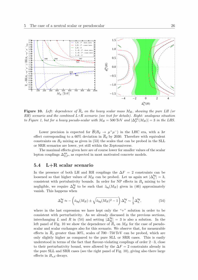
Then by using the formulae listed above we can calculate the ratio Rq of B̄(Bq →µ+µ−) to its SM expectation, given in (88), as a function of MH . From Table 1we see that in 2024 a deviation of 3σ from the SM estimate of B(Bs → µ+µ−) willcorrespond to a 30% deviation in Rs from one. In the left panel of Fig. 10 we showthe dependence of Rs on MH for the case of pseudo-scalar and scalar exchanges. Weobserve that measurable effects of pseudo-scalar exchanges can be obtained at MH
as high as 600 – 700 TeV for the large couplings considered, which is also dependenton constructive or destructive interference with the SM. Because scalars do notinterfere with the SM contributions, they only just approach the Zeptouniversescale of 200 TeV.
In the right panel of Fig. 10 we show the result of a fit of all the ∆F = 2constraints for an arbitrary phase of the ∆bs
L (H) coupling – i.e. allowing for CPviolation in the scalar sector – together with the projections for B̄(Bs → µ+µ−)in 2019 and 2024, in the plane 9 ∆bs
L (H)–φbsL (H). The notation is the same as inFig. 1, with the green regions being allowed by the ∆F = 2 fit at 68% and 95% C.L.,and the continuous and dashed lines indicating 3σ and 5σ effects in Bs → µ+µ−,respectively. We fixed MH = 500 TeV and |∆µµ
P | = 3. The effects are maximal forreal, positive values of the coupling, where there is maximal constructive interferencewith the SM contribution.
9Writing the ∆bqL (H) coupling as i∆bq
L (H)eiφbqL (H)
5 The case of a neutral scalar or pseudoscalar 26
0 100 200 300 400 500 600 700 800 900 1000
MH [TeV]
0.00.10.20.30.40.50.60.70.80.91.01.11.21.31.41.51.61.71.81.92.02.12.2
Rs=
BR
(Bs→µ
+µ−
)/B
R(B
s→µ
+µ−
) SM
619
723
168
691
747358
L/R : P −destr. inter.
L/R : P −const. inter.
L/R : S
L +R : P −destr. inter.
L +R : P −const. inter.
L +R : S
-4 -2 0 2 4
-1.5
-1.0
-0.5
0.0
0.5
1.0
1.5
DLbsHHL
ΦLbs
HHL
Figure 10. Left: dependence of Rs on the heavy scalar mass MH , showing the pure LH (orRH) scenario and the combined L+R scenario (see text for details). Right: analogous situationto Figure 1, but for a heavy pseudo-scalar with MH = 500 TeV and |∆µµ
P (MH)| = 3 in the LHS.
Lower precision is expected for B(Bd → µ+µ−) in the LHC era, with a 3σeffect corresponding to a 60% deviation in Rd by 2030. Therefore with equivalentconstraints on Bd mixing as given in (53) the scales that can be probed in the SLLor SRR scenarios are lower, yet still within the Zeptouniverse.
The maximal effects given here are of course lower for smaller values of the scalarlepton couplings ∆µµ
S,P , as expected in most motivated concrete models.
5.4 L+R scalar scenario
In the presence of both LH and RH couplings the ∆F = 2 constraints can beloosened so that higher values of MH can be probed. Let us again set |∆bq
L | = 3,consistent with pertubativity bounds. In order for NP effects in Bq mixing to be
negligible, we require ∆bqR to be such that z̃bq(MH) given in (46) approximately
vanish. This happens when
∆bqR ≈ −
(κ̃bq(MH)±
√κ̃bq(MH)2 − 1
)∆bqL ∼
1
5∆bqL , (54)
where in the last expression we have kept only the “+” solution in order to beconsistent with perturbativity. As we already discussed in the previous sections,interchanging L and R in (54) and setting |∆bq
R | = 3 is also a solution. In theleft panel of Fig. 10 we show the dependence of Rs on MH for the case of pseudo-scalar and scalar exchanges also for this scenario. We observe that, for measurableeffects in Rs greater than 30%, scales of 700 – 750 TeV can be probed, which areonly slightly higher as compared to the pure SLL or SRR cases. This is easilyunderstood in terms of the fact that flavour-violating couplings of order 2 – 3, closeto their perturbativity bound, were allowed by the ∆F = 2 constraints already inthe pure SLL and SRR cases (see the right panel of Fig. 10), giving also there largeeffects in Bs,d decays.
6 Other New Physics scenarios 27
In contrast, for NP effects that give a Rd greater than 60%, which could beobservable at 3σ in 2030, the additional smallness of the B(Bd → µ+µ−) SM esti-mate (due to |Vtd| � |Vts|) allows scales up to 1200 TeV to be probed for the largecouplings we consider.
6 Other New Physics scenarios
6.1 Preliminaries
We would like now to address the question whether our findings can be generalisedto other NP scenarios while keeping in mind that we would like to obtain the highestpossible resolution of short distance scales with the help of ∆F = 1 processes andstaying consistent with the constraints from ∆F = 2 processes and perturbativity.After all our NP scenarios up till now have been very simple: one heavy gaugeboson or (pseudo-)scalar contributing to both ∆F = 1 and ∆F = 2 transitions attree-level. In general one could have several new particles and, moreover, there isthe possibility of a GIM mechanism at work protecting against FCNCs at tree-level.Before discussing various possibilities let us make a few general observations:
• If a gauge boson or scalar (pseudoscalar) contributes at tree-level to ∆F = 1transitions it will necessarily contribute also to ∆F = 2 transitions.
• On the other hand a gauge boson or a scalar (pseudoscalar) can contributeto ∆F = 2 transitions at tree-level without having any impact on ∆F = 1transitions. This is the case, for instance, for a heavy gluon G′, which, carryingcolour, does not couple to leptons, or for a leptophobic Z ′. In the case of ascalar (pseudoscalar) this could be realised if the coupling of these bosons toleptons is suppressed through small lepton masses, which is the case if thesebosons take part in electroweak symmetry breaking.
We will now briefly discuss two large classes of NP models, reaching the followingconclusions:
• In order to achieve a high resolution of short-distance scales in the presence oftree-level FCNCs that satisfy ∆F = 2 constraints, one generally has to breakthe correlation between ∆F = 1 and ∆F = 2 transitions. In the case of asingle Z ′ or (pseudo-)scalar this can be done via the L+R scenario, or by theintroduction of multiple such NP particles.10
• If the GIM mechanism is at work and there are no tree-level FCNCs thepattern of correlations between ∆F = 1 and ∆F = 2 transitions could bedifferent than in the case of tree-level FCNCs. Yet, as we will show, in thiscase the energy scales which can be explored by rare K and Bs,d decays aresignificantly lower than the ones found by us in the previous sections.
6.2 The case of two gauge bosons
Let us assume that there are two gauge bosons Z ′1 and Z ′2 but only Z ′1 couples toleptons i.e. Z ′2 could be colourless or an octet of SU(3)c. In such a model it is
10 In special cases such as the decays K+ → π+νν̄ and KL → π0νν̄ in Z ′ scenarios, and Bs,d → µ+µ−
in the scalar case, the Zeptouniverse can be reached even in the presence of ∆F = 2 constraints.
6 Other New Physics scenarios 28
possible to reach very high scales with only LH or RH couplings to quarks. Indeed,let us assume that these two bosons have only LH flavour violating couplings. OnlyZ ′1 is relevant for ∆F = 1 transitions and if Z ′2 were absent we would have the LHscenario of Section 3, which does not allow measurable effects in Bs,d decays above20 TeV due to ∆F = 2 constraints.
On the contrary, with two gauge bosons we can suppress NP contributions to∆F = 2 transitions by choosing their couplings and masses such that their contri-butions to ∆Ms,d approximately cancel. This is clearly a tuned scenario. Assumingthat the masses of these bosons are of the same order so that we can ignore thedifferences in RG QCD effects, a straightforward calculation allows us to derive therelation [
∆ijL (Z ′1)
∆ijL (Z ′2)
]2
= − 1
Nc
[MZ′1
MZ′2
]2
(55)
which should be approximately satisfied. Here Nc is equal to 3 or 1 for Z ′2 with orwithout colour, respectively. This in turn implies
∆ijL (Z ′2) = i
√Nc ∆ij
L (Z ′1)
[MZ′2
MZ′1
](56)
so that the phases of these couplings must differ by π.The same argument can be made for RH couplings. Moreover, it is not required
that both gauge bosons have LH or RH couplings and the relation in (56) assurescancellation of NP contributions to ∆F = 2 processes for the four possibilities ofchoosing different couplings. The two scenarios for Z ′1 can be distinguished by raredecays. One can of course also consider L+R scenario but it is not necessary here.
In the case of two gauge bosons with comparable masses also scenarios could beconsidered in which these bosons have LH and RH couplings of roughly the samesize properly tuned to minimise constraints from ∆F = 2 observables. However, ifperturbativity for their couplings is assumed the highest resolution of short distancescales will still be comparable to the one found in the previous section. On theother hand with two gauge bosons having LH and RH couplings of the same size,the correlations between ∆F = 1 observables could be modified with respect to theones presented in our paper. We will return to this possibility in the future.
6.3 The case of a degenerate scalar and pseudo-scalarpair
We proceed to consider a model consisting of a scalar H0 and a pseudo-scalar A0
with equal (or nearly degenerate) mass MH0 = MA0 = MH . This is, for example,essentially realised for 2HDMs in a decoupling regime, where H0 and A0 are muchheavier than the SM Higgs h0 and almost degenerate in mass. Allowing for a scalarH0 and pseudo-scalar A0 with equal couplings to quarks, i.e.
L 3 DL∆̃DR(H0 + iA0) + h.c, (57)
where D = (d, s, b) and ∆̃ is a matrix in flavour space, gives the couplings
∆qbR (H0) = ∆̃qb, ∆qb
R (A0) = i∆̃qb, ∆qbL (H0) =
(∆̃bq
)∗, ∆qb
L (A0) = −i(∆̃bq
)∗.
(58)
7 Can we determine MZ′ beyond the LHC scales? 29
Restricting the couplings to be purely LH or RH and assuming a degenerate mass,we see from inspection of (42) that the contributions to (M∗12)bqH will automaticallycancel, without fine-tuning in the couplings. However, if both LH and RH couplingsare present, the LR operator will contribute to the mixing. In 2HDMs with MFV,for example, the ∆qb
L couplings are suppressed by mq/mb relative to ∆qbR , which will
give small but non-zero contributions to the mixing even in the limit of a degenerateheavy neutral scalar and pseudoscalar.
Let us consider the case of only LH (or RH) couplings, and set |∆sbL | = |∆
µµP | =
3.0 as before. Then, for observable deviations in Rs greater than 30%, we find thatthis model can probe scales up to MH = 850 TeV, which is comparable to the twoscenarios discussed in Sections 5.3 and 5.4.
6.4 GIM case
If there are no FCNCs at the tree-level, then new particles entering various boxand penguin diagrams enter the game, making the correlations between ∆F = 1and ∆F = 2 processes more difficult to analyse. However, it is evident that for thesame couplings NP effects in this case will be significantly suppressed relative tothe scenarios discussed until now. This is good for suppressing NP contributions atrelative low scales but it does not allow us to reach energy scales as high as in thecase of FCNCs at the tree level.
Assuming that the involved one-loop functions are O(1) and comparing tree-levelexpressions for ∆F = 2 and ∆F = 1 effective Hamiltonians with those one wouldtypically get by calculating box and penguin diagrams we find that NP contributionsfrom loop diagrams are suppressed relative to tree diagrams by the additional factors
κ(∆F = 2) =∆2L,R
32π2, κ(∆F = 1) =
∆2L,R
8π2. (59)
For couplings ∆L,R ≈ 3 these suppressions amount approximately to 1/40 and 1/10respectively. This in turn implies that at the same precision as in the previoussections the maximal scales at which NP could be studied are reduced by roughlyfactors of 6 and 3 for ∆F = 2 and ∆F = 1, respectively. For smaller couplings thisreduction is larger. Detail numbers are not possible without the study of a concretemodel.
7 Can we determine MZ′ beyond the LHC
scales?
We have seen that all observables considered in Z ′ scenarios depend on the ratiosof the Z ′ couplings over the Z ′ mass MZ′ as listed in (1) and (2). By assuming thelargest couplings consistent with perturbativity we have succeeded to give an ideaabout the highest values of MZ′ that could still allow us to study the structure ofthe NP involved. However it is not guaranteed that the Z ′ couplings are that largeand MZ′ could also be smaller, yet still significantly higher than the LHC scales.
Let us therefore assume that in the future all observables considered in our paperhave been measured with high precision and all CKM and hadronic uncertainties
8 Conclusions 30
have been reduced to a few percent level. Moreover, let us assume significant depar-tures from SM predictions have been identified with the pattern of deviations fromthe SM pointing towards the existence of a heavy Z ′. We then ask the questionwhether in this situation we could determine at least approximately the value ofMZ′ on the basis of flavour observables.
Before we answer this question let us recall that the masses of the SM gaugebosons Z and W± were predicted in the 1970’s, several years before their discov-ery, due to the knowledge of GF , αem and sin2 θW - all determined in low energyprocesses. Similarly also the masses of the charm quark and top quark could beapproximately predicted. Yet, this was only possible because it was done within aconcrete theory, the SM, which allowed one to use all measured low energy processesat that time. Thus within a specific theory with not too many free parameters, onecould imagine that also the mass of Z ′ could be indirectly determined. But what ifthe only information about Z ′ comes from the processes considered by us?
Here we would like to point out the possibility of determining MZ′ from flavourobservables provided the next e+e− or µ+µ− collider, still with center of massenergies well below MZ′ , could determine indirectly the leptonic ratios in (2). Thiswill only be possible if in these collisions some departures from SM expectationswill also be found. Only the determination of the ratios involving muon couplingsis necessary as the one involving neutrino couplings could be obtained throughthe SU(2)L relation in (2). These ratios could of course be obtained from theupgraded LHC, but the presence of protons in the initial state will complicate thisdetermination.
Knowing the values of the ratios in (2), one could determine all ratios in (1)through rare K and Bs,d decays. Here the decays governed by b → s transitionsare superior to the other decays as there are many of them, yet if the decays KL →π0`+`− could be measured and the hadronic matrix elements entering ε′/ε broughtunder control also the K system would be of interest here.
What is crucial for the idea that follows is that ∆F = 2 transitions have notyet been used for the determination of the ratios in (1), that both LH and RH arepresent, and that both are relevant for rare decays to the extent that the ratios in(1) can be measured. This would not allow the resolution of the highest scales butwould still provide interesting results.
Now for the main point. With the ratios in (1) determined by rare decays,the dependence of the right-hand sides of (32) and (33) on MZ′ is only throughthe hadronic matrix elements of the involved operators. Although this dependence,as given in Table 5, is only logarithmic, it is sufficiently strong in the presence ofLR operators to allow one to estimate the value of MZ′ with the help of ∆F = 2observables. To this end precise knowledge of the relevant hadronic matrix elementsis necessary. This also applies to CKM parameters entering SM contributions. Inprinciple the same discussions can be made for scalars but it is unlikely that theycan play a prominent role in e+e− collisions.
8 Conclusions
In this paper we have addressed the question of whether we could learn somethingabout the very short distance scales that are beyond the reach of the LHC on thebasis of quark flavour observables alone. Certainly this depends on the size of
8 Conclusions 31
NP, its nature and in particular on the available precision of the SM predictionsfor flavour observables. The latter precision depends on the extraction of CKMparameters from the data and on the theoretical uncertainties. Both are expectedto be reduced in this decade down to 1 – 2%, which should allow NP to be identifiedeven if it contributed only at the level of 10 – 30% to the branching ratios.
Answering this question in the context of Z ′ models and assuming that all itscouplings to SM fermions take values of at most 3.0, our main findings are as follows:
• ∆F = 2 processes alone cannot give us any concrete information about thenature of NP at short distance scales beyond the reach of the LHC. In par-ticular if some deviations from SM expectations will be observed, it will notbe possible to find out whether they come from LH currents, RH currents orboth.
• On the other hand future precise measurements of several ∆F = 1 observ-ables and in particular correlations between them can distinguish between LHand RH currents, but the maximal resolution consistent with perturbativitystrongly depends on whether only LH or only RH or both LH and RH flavourchanging Z ′ couplings to quarks are present in nature.
• If only LH or RH couplings are present in nature we can in principle reach scalesof 200 TeV and 15 TeV for K and Bs,d, respectively. These numbers depend onthe room left for NP in ∆F = 2 observables, which have an important impacton the resolution available in these NP scenarios.
• Smaller distance scales can only be resolved if both RH and LH couplings arepresent in order to cancel the NP effects on the ∆F = 2 observables. Moreover,to achieve the necessary tuning, the couplings should differ considerably fromeach other. This large hierarchy of couplings is dictated primarily by the ratioof hadronic matrix elements of LR ∆F = 2 operators and those for LL and RRoperators and by the room left for NP in ∆F = 2 processes. We find that inthis case the scales as high as 2000 TeV and 160 TeV for K and Bs,d systems,respectively, could be in principle resolved.
• A study of tree-level (pseudo-)scalar exchanges shows that Bs,d → µ+µ− canprobe scales close to 1000 TeV, both for scenarios with purely LH or RH scalarcouplings to quarks and for scenarios allowing for both LH and RH couplings.For the limit of a degenerate scalar and pseudoscalar NP effects in ∆F = 2observables can cancel even without imposing a tuning on the couplings.
• We have discussed models with several gauge bosons. Also in this case thebasic strategy for being able to explore very high energy scales is to break thestringent correlation between ∆F = 1 and ∆F = 2 processes and to suppressNP contributions to the latter without suppressing NP contributions to raredecays. The presence of a second heavy neutral gauge boson allows us toachieve the goal with only LH or RH currents by applying an appropriatetuning.
• While the highest achievable resolution in the presence of several gauge bosonsis comparable to the case of a single gauge boson because of the perturbativitybound, the correlations between ∆F = 1 observables could differ from the onespresented here. This would be in particular the case if LH and RH couplingsof these bosons where of similar size. A detailed study of such scenarios wouldrequire the formulation of concrete models.
A ∆F = 1 master functions 32
• If FCNCs only occur at one loop level the highest energy scales that can beresolved for maximal couplings are typically reduced relative to the case oftree-level FCNCs by a factor of at least 3 and 6 for ∆F = 1 and ∆F = 2processes, respectively.
• We have also presented a simple idea for a rough indirect determination of MZ′
by means of the next linear e+e− or µ+µ− collider and precision flavour data.It uses the fact that the LR operators present in ∆F = 2 transitions have largeanomalous dimensions so that MZ′ can be determined through renormalisationgroup effects provided it is well above the LHC scales.
In summary we have demonstrated that NP with a particular pattern of dynam-ics could be investigated through rare K and Bs,d decays even if the scale of thisNP would be close to the Zeptouniverse. As expected from other studies it is inprinciple easier to reach the Zeptouniverse with the help of rare K decays than Bs,ddecays. However, this assumes the same maximal couplings in these three systemsand this could be not the case. Moreover, in the presence of tree-level pseudoscalarexchanges very short distance scales can be probed by Bs,d → µ+µ− decays.
We should also emphasise that although our main goal was to reach the highestenergy scales with the help of rare decays, it will of course be exciting to explore anyscale of NP above the LHC scales in this decade. Moreover, we still hope that highenergy proton-proton collisions at the LHC will exhibit at least some foot prints ofnew particles and forces. This would greatly facilitate flavour analyses as the onepresented here.
Acknowledgements
This research was done and financed in the context of the ERC Advanced Grantproject “FLAVOUR”(267104) and was partially supported by the DFG cluster ofexcellence “Origin and Structure of the Universe”.
A ∆F = 1 master functions
Here we collect the ∆F = 1 functions that enter the various rare K and Bs,ddecays discussed in this paper. We do not give the more complicated expressionsfor NP contributions to ∆F = 2 observables. They can be found in Section 3.2.1of [16]. Note that we have updated the relevant hadronic matrix elements, as givenin Table 5.
The master functions in question that enter our analysis are given as follows [16]:
XL(K) = ηXX0(xt) +∆νν̄L
g2SMM
2Z′
∆sdL
V ∗tsVtd, (60)
XR(K) =∆νν̄L
g2SMM
2Z′
∆sdR
V ∗tsVtd, (61)
XL(Bq) = ηXX0(xt) +
[∆ννL
M2Z′g
2SM
]∆qbL
V ∗tqVtb, (62)
XR(Bq) =
[∆ννL
M2Z′g
2SM
]∆qbR
V ∗tqVtb, (63)
B Basic formulae for observables 33
YA(K) = ηY Y0(xt) +
[∆µµ̄A
]M2Z′g
2SM
[∆sdL −∆sd
R
V ?tsVtd
]≡ |YA(K)|eiθKY , (64)
YA(Bq) = ηY Y0(xt) +
[∆µµ̄A
]M2Z′g
2SM
[∆qbL −∆qb
R
V ?tqVtb
]≡ |YA(Bq)|eiθ
BqY . (65)
Here ηX,Y are factors which include both QCD corrections [96–98] and NLO elec-troweak correction [99–101]. For mt = mt(mt) they are close to unity ,
ηX = 0.994, ηY = 0.9982 . (66)
gSM is defined in (12). Explicit expressions for the SM functions X0(xt) and Y0(xt)can be found in [1].
B Basic formulae for observables
B.1 Operators
We list here the operators that contribute to ∆F = 2 observables. Specifically, forthe B0
q − B̄0q system the full basis is given as follows [1, 87,88]:
QVLL1 =
(b̄γµPLq
) (b̄γµPLq
), QVRR
1 =(b̄γµPRq
) (b̄γµPRq
), (67)
QLR1 =
(b̄γµPLq
) (b̄γµPRq
), QLR
2 =(b̄PLq
) (b̄PRq
), (68)
QSLL1 =
(b̄PLq
) (b̄PLq
), QSRR
1 =(b̄PRq
) (b̄PRq
), (69)
QSLL2 =
(b̄σµνPLq
) (b̄σµνPLq
), QSRR
2 =(b̄σµνPRq
) (b̄σµνPRq
), (70)
where PR,L = (1± γ5)/2. Colour indices are suppressed as they are summed up ineach factor. For K0 − K̄0 mixing b↔ s and q ↔ d have to be interchanged.
B.2 K+ → π+νν̄ and KL → π0νν̄
The branching ratios for these two modes can be written in the general form
B(K+ → π+νν̄) = κ+
[(ImXeff
λ5
)2
+
(ReXeff
λ5− P̄c(X)
)2], (71)
B(KL → π0νν̄) = κL
(ImXeff
λ5
)2
, (72)
with the Cabibbo angle λ = 0.2252(9) and where [102]
κ+ = (5.21±0.025)·10−11
(λ
0.2252
)8
, κL = (2.25±0.01)·10−10
(λ
0.2252
)8
, (73)
and [102–106]
P̄c(X) =
(1− λ2
2
)Pc(X), Pc(X) = (0.42± 0.03)
(0.2252
λ
)4
. (74)
The short distance contributions are described by
Xeff = V ∗tsVtd(XL(K) +XR(K)
), (75)
where XL,R(K) are given in (60) and (61).
B Basic formulae for observables 34
B.3 B → {Xs,K,K∗}νν̄
The branching ratios of the B → {K,K∗}νν̄ modes in the presence of RH currentscan be written as follows [81]
B(B → Kνν̄)
B(B → Kνν̄)SM= [1− 2η] ε2 , (76)
B(B → K∗νν̄)
B(B → K∗νν̄)SM= [1 + 1.31η] ε2 , (77)
where
ε2 =|XL(Bs)|2 + |XR(Bs)|2
|ηXX0(xt)|2, η =
−Re (XL(Bs)X∗R(Bs))
|XL(Bs)|2 + |XR(Bs)|2, (78)
with XL,R(Bs) defined in (62) and (63).
B.4 KL → µ+µ−
Only the so-called short distance (SD) part to a dispersive contribution to KL →µ+µ− can be reliably calculated but it serves as a useful constraint on NP contribut-ing to K+ → π+νν̄. It is given by
B(KL → µ+µ−)SD = κµ
(ReYeff
λ5− P̄c(Y )
)2
. (79)
Here
κµ = (2.01± 0.02) · 10−9
(λ
0.2252
)8
, Yeff = V ∗tsVtdYA(K), (80)
where YA(K) is given in (64) and
P̄c (Y ) =
(1− λ2
2
)Pc (Y ) , Pc (Y ) = (0.115± 0.018)
(0.2252
λ
)4
, (81)
with Pc (Y ) at NNLO [107]. The extraction of the short distance part from the datais subject to considerable uncertainties. The most recent estimate gives [108]
B(KL → µ+µ−)SD ≤ 2.5 · 10−9 , (82)
to be compared with (0.8± 0.1) · 10−9 in the SM [107].
B.5 B → K(∗)`+`−
The effective Hamiltonian for b → s`+`− transitions, such as B → K∗`+`−, B →K`+`− and B → Xs`
+`−, is given as (see e.g. also [94])
Heff(b→ s`¯̀) = Heff(b→ sγ)−4GF√2
α
4πV ∗tsVtb
∑i=9,10,S,P
[Ci(µ)Qi(µ)+C ′i(µ)Q′i(µ)] (83)
where
Q9 = (s̄γµPLb)(¯̀γµ`), Q′9 = (s̄γµPRb)(¯̀γµ`), (84)
Q10 = (s̄γµPLb)(¯̀γµγ5`), Q′10 = (s̄γµPRb)(¯̀γµγ5`), (85)
QS = mb(s̄PRb)(¯̀̀ ), Q′S = mb(s̄PLb)(¯̀̀ ), (86)
QP = mb(s̄PRb)(¯̀γ5`), Q′P = mb(s̄PLb)(¯̀γ5`). (87)
References 35
B.6 Bd,s → µ+µ−
The ratio of the Bq → µ+µ− branching ratio, with q = s, d, relative to its SMestimate is given by [94,109]
Rq ≡B(Bq → µ+µ−)
B(Bq → µ+µ−)SM
=
[1 +Aµµ∆Γ(Bq → µ+µ−) yq
1 + yq
] (|P |2 + |S|2
), (88)
where
P ≡ −YA(Bq)
sin2 θWCSM10
+m2Bq
2mµ
mb
mb +mq
CP − C ′PCSM
10
, (89)
S ≡
√1−
4m2µ
m2Bq
m2Bq
2mµ
mb
mb +mq
CS − C ′SCSM
10
, (90)
with CSM10 = −ηY sin−2 θWY0(xt) the only relevant coefficient in the SM and YA(Bq)
given in (65). The coefficients C(′)P and C
(′)S correspond to the effective (pseudo-
)scalar operators given in (87) and (86), respectively. Aµµ∆Γ(Bq → µ+µ−) is themass-eigenstate rate asymmetry for this decay, which is relevant in the case of anon-zero Bq lifetime difference yq = (τq,H − τq,L)/(τq,H + τq,L) [110] i.e. for the Bsdecay where ys is non-zero.
In the SM only the heavy mass-eigenstate contributes to these decays, giving amaximal asymmetry, Aµµ∆Γ = 1, and thereby a maximal correction to the branchingratio. In Z ′ models this asymmetry only differs from its SM value in the presenceof new CP violating phases, whereas in models with new scalars it can deviate fromone also in the absence of such phases [93,109].
References
[1] A. J. Buras and J. Girrbach, Towards the Identification of New Physicsthrough Quark Flavour Violating Processes, Rept.Prog.Phys. 77 (2014)086201, [arXiv:1306.3775].
[2] G. Isidori and F. Teubert, Status of indirect searches for New Physics withheavy flavour decays after the initial LHC run, Eur.Phys.J.Plus 129 (2014)40, [arXiv:1402.2844].
[3] UTfit Collaboration, M. Bona et. al., Model-independent constraints on ∆F=2 operators and the scale of new physics, JHEP 0803 (2008) 049,[arXiv:0707.0636]. Updates available on http://www.utfit.org.
[4] G. Isidori, Y. Nir, and G. Perez, Flavor Physics Constraints for PhysicsBeyond the Standard Model, Ann.Rev.Nucl.Part.Sci. 60 (2010) 355,[arXiv:1002.0900].
[5] J. Charles, S. Descotes-Genon, Z. Ligeti, S. Monteil, M. Papucci, et. al.,Future sensitivity to new physics in Bd, Bs and K mixings, Phys.Rev. D89(2014) 033016, [arXiv:1309.2293].
[6] J. Hewett, H. Weerts, R. Brock, J. Butler, B. Casey, et. al., FundamentalPhysics at the Intensity Frontier, arXiv:1205.2671.
References 36
[7] J. Engel, M. J. Ramsey-Musolf, and U. van Kolck, Electric Dipole Momentsof Nucleons, Nuclei, and Atoms: The Standard Model and Beyond,Prog.Part.Nucl.Phys. 71 (2013) 21–74, [arXiv:1303.2371].
[8] D. McKeen, M. Pospelov, and A. Ritz, Electric dipole moment signatures ofPeV-scale superpartners, Phys.Rev. D87 (2013), no. 11 113002,[arXiv:1303.1172].
[9] T. Moroi and M. Nagai, Probing Supersymmetric Model with HeavySfermions Using Leptonic Flavor and CP Violations, Phys.Lett. B723(2013) 107–112, [arXiv:1303.0668].
[10] T. Moroi, M. Nagai, and T. T. Yanagida, Lepton Flavor Violations inHigh-Scale SUSY with Right-Handed Neutrinos, Phys.Lett. B728 (2014)342–346, [arXiv:1305.7357].
[11] L. Eliaz, A. Giveon, S. B. Gudnason, and E. Tsuk, Mild-split SUSY withflavor, JHEP 1310 (2013) 136, [arXiv:1306.2956].
[12] A. S. Kronfeld, R. S. Tschirhart, U. Al-Binni, W. Altmannshofer,C. Ankenbrandt, et. al., Project X: Physics Opportunities,arXiv:1306.5009.
[13] A. de Gouvea and P. Vogel, Lepton Flavor and Number Conservation, andPhysics Beyond the Standard Model, Prog.Part.Nucl.Phys. 71 (2013) 75–92,[arXiv:1303.4097].
[14] R. H. Bernstein and P. S. Cooper, Charged Lepton Flavor Violation: AnExperimenter’s Guide, Phys.Rept. 532 (2013) 27–64, [arXiv:1307.5787].
[15] W. Altmannshofer, R. Harnik, and J. Zupan, Low Energy Probes of PeVScale Sfermions, JHEP 1311 (2013) 202, [arXiv:1308.3653].
[16] A. J. Buras, F. De Fazio, and J. Girrbach, The Anatomy of Z’ and Z withFlavour Changing Neutral Currents in the Flavour Precision Era, JHEP1302 (2013) 116, [arXiv:1211.1896].
[17] A. J. Buras and J. Girrbach, Left-handed Z’ and Z FCNC quark couplingsfacing new b→ sµ+µ− data, JHEP 1312 (2013) 009, [arXiv:1309.2466].
[18] A. J. Buras, F. De Fazio, J. Girrbach, and M. V. Carlucci, The Anatomy ofQuark Flavour Observables in 331 Models in the Flavour Precision Era,JHEP 1302 (2013) 023, [arXiv:1211.1237].
[19] A. J. Buras, F. De Fazio, and J. Girrbach, 331 models facing newb→ sµ+µ− data, JHEP 1402 (2014) 112, [arXiv:1311.6729].
[20] A. J. Buras, F. De Fazio, and J. Girrbach-Noe, Z-Z’ mixing and Z-mediatedFCNCs in SU(3)C × SU(3)L × U(1)X Models, JHEP 1408 (2014) 039,[arXiv:1405.3850].
[21] R. S. Chivukula and H. Georgi, Composite technicolor standard model, Phys.Lett. B188 (1987) 99.
[22] L. J. Hall and L. Randall, Weak scale effective supersymmetry, Phys. Rev.Lett. 65 (1990) 2939–2942.
[23] G. D’Ambrosio, G. F. Giudice, G. Isidori, and A. Strumia, Minimal flavourviolation: An effective field theory approach, Nucl. Phys. B645 (2002)155–187, [hep-ph/0207036].
References 37
[24] R. Barbieri, G. Isidori, J. Jones-Perez, P. Lodone, and D. M. Straub, U(2)and Minimal Flavour Violation in Supersymmetry, Eur.Phys.J. C71 (2011)1725, [arXiv:1105.2296].
[25] R. Barbieri, D. Buttazzo, F. Sala, and D. M. Straub, Flavour physics froman approximate U(2)3 symmetry, JHEP 1207 (2012) 181,[arXiv:1203.4218].
[26] R. Barbieri, D. Buttazzo, F. Sala, and D. M. Straub, Less Minimal FlavourViolation, JHEP 1210 (2012) 040, [arXiv:1206.1327].
[27] R. Barbieri, D. Buttazzo, F. Sala, D. M. Straub, and A. Tesi, A 125 GeVcomposite Higgs boson versus flavour and electroweak precision tests, JHEP1305 (2013) 069, [arXiv:1211.5085].
[28] T. Feldmann and T. Mannel, Minimal Flavour Violation and Beyond, JHEP0702 (2007) 067, [hep-ph/0611095].
[29] T. Hurth, G. Isidori, J. F. Kamenik, and F. Mescia, Constraints on NewPhysics in MFV models: A Model-independent analysis of ∆F =1 processes,Nucl. Phys. B808 (2009) 326–346, [arXiv:0807.5039].
[30] G. Isidori and D. M. Straub, Minimal Flavour Violation and Beyond,Eur.Phys.J. C72 (2012) 2103, [arXiv:1202.0464].
[31] A. J. Buras, F. De Fazio, and J. Girrbach, ∆I = 1/2 rule, ε′/ε andK → πνν̄ in Z ′(Z) and G′ models with FCNC quark couplings, Eur.Phys.J.C74 (2014) 2950, [arXiv:1404.3824].
[32] E949 Collaboration, A. V. Artamonov et. al., New measurement of theK+ → π+νν̄ branching ratio, Phys. Rev. Lett. 101 (2008) 191802,[arXiv:0808.2459].
[33] G. Anelli, A. Ceccucci, V. Falaleev, F. Formenti, A. Gonidec, et. al.,Proposal to measure the rare decay K+ → π+νν̄ at the CERN SPS, .
[34] Quark Flavor Physics Working Group Collaboration, J. Butler et. al.,Report of the Quark Flavor Physics Working Group, arXiv:1311.1076.
[35] E391a Collaboration, J. Ahn et. al., Experimental study of the decayK0L → π0νν̄, Phys.Rev. D81 (2010) 072004, [arXiv:0911.4789].
[36] BaBar Collaboration, P. del Amo Sanchez et. al., Search for the Rare DecayB → Kνν̄, Phys.Rev. D82 (2010) 112002, [arXiv:1009.1529].
[37] T. Aushev, W. Bartel, A. Bondar, J. Brodzicka, T. Browder, et. al., Physicsat Super B Factory, arXiv:1002.5012.
[38] Belle Collaboration, O. Lutz et. al., Search for B → h(∗)νν̄ with the fullBelle Y(4S) data sample, Phys.Rev. D87 (2013) 111103, [arXiv:1303.3719].
[39] LHCb Collaboration, R. Aaij et. al., Measurement of the B0s → µ+µ−
branching fraction and search for B0 → µ+µ− decays at the LHCbexperiment, Phys.Rev.Lett. 111 (2013) 101805, [arXiv:1307.5024].
[40] CMS Collaboration, S. Chatrchyan et. al., Measurement of the Bs → µµbranching fraction and search for B0 → µµ with the CMS Experiment,Phys.Rev.Lett. 111 (2013) 101804, [arXiv:1307.5025].
References 38
[41] CMS and LHCb Collaboration, Combination of results on the rare decaysB0
(s) → µ+µ− from the CMS and LHCb experiments,
CMS-PAS-BPH-13-007, LHCb-CONF-2013-012 (2013).
[42] CMS Collaboration, CMS reach in B[s] to dimuon and B to dimuonbranching fractions for the new LHC runs, .http://cds.cern.ch/record/1605250.
[43] LHCb Collaboration, R. Aaij et. al., Implications of LHCb measurementsand future prospects, EPJ C 73 (2013) 2373, [arXiv:1208.3355].
[44] S. Aoki, Y. Aoki, C. Bernard, T. Blum, G. Colangelo, et. al., Review oflattice results concerning low energy particle physics, arXiv:1310.8555.
[45] USQCD Collaboration, T. Blum, M. Bucho, N. Christ, A. Kronfeld,P. Mackenzie, S. Sharpe, R. Sugar, and R. Van de Water, Lattice QCD atthe Intensity Frontier, . http://usqcd.org/documents/13flavor.pdf.
[46] T. Blum, R. Van de Water, D. Holmgren, R. Brower, S. Catterall, et. al.,Working Group Report: Lattice Field Theory, arXiv:1310.6087.
[47] P. Gambino and C. Schwanda, Inclusive semileptonic fits, heavy quarkmasses, and Vcb, Phys.Rev. D89 (2014) 014022, [arXiv:1307.4551].
[48] G. Ricciardi, Determination of the CKM matrix elements —V(xb)—,Mod.Phys.Lett. A28 (2013) 1330016, [arXiv:1305.2844].
[49] UTfit Collaboration. http://www.utfit.org.
[50] Heavy Flavor Averaging Group (HFAG) Collaboration, E. Barberioet. al., Averages of b−hadron properties at the end of 2006,arXiv:0704.3575.
[51] S. Faller, M. Jung, R. Fleischer, and T. Mannel, The Golden ModesB0 → J/ψKS,L in the Era of Precision Flavour Physics, Phys.Rev. D79(2009) 014030, [arXiv:0809.0842].
[52] M. Ciuchini, M. Pierini, and L. Silvestrini, Theoretical uncertainty in sin 2β:An Update, arXiv:1102.0392.
[53] S. Faller, R. Fleischer, and T. Mannel, Precision Physics with B0s → J/ψφ at
the LHC: The Quest for New Physics, Phys.Rev. D79 (2009) 014005,[arXiv:0810.4248].
[54] Particle Data Group Collaboration, K. Nakamura et. al., Review ofparticle physics, J.Phys.G G37 (2010) 075021.
[55] Particle Data Group Collaboration, J. Beringer et. al., Review of ParticlePhysics (RPP), Phys.Rev. D86 (2012) 010001.
[56] Heavy Flavor Averaging Group Collaboration, Y. Amhis et. al.,Averages of B-Hadron, C-Hadron, and tau-lepton properties as of early 2012,arXiv:1207.1158. http://www.slac.stanford.edu/xorg/hfag.
[57] K. Chetyrkin, J. Kuhn, A. Maier, P. Maierhofer, P. Marquard, et. al.,Charm and Bottom Quark Masses: An Update, Phys.Rev. D80 (2009)074010, [arXiv:0907.2110].
[58] J. Laiho, E. Lunghi, and R. S. Van de Water, Lattice QCD inputs to theCKM unitarity triangle analysis, Phys. Rev. D81 (2010) 034503,[arXiv:0910.2928]. Updates available on http://latticeaverages.org/.
References 39
[59] HPQCD Collaboration, I. Allison et. al., High-Precision Charm-QuarkMass from Current-Current Correlators in Lattice and Continuum QCD,Phys.Rev. D78 (2008) 054513, [arXiv:0805.2999].
[60] HPQCD Collaboration, R. Dowdall, C. Davies, R. Horgan, C. Monahan,and J. Shigemitsu, B-meson decay constants from improved lattice NRQCDand physical u, d, s and c sea quarks, Phys.Rev.Lett. 110 (2013) 222003,[arXiv:1302.2644].
[61] A. J. Buras and D. Guadagnoli, Correlations among new CP violating effectsin ∆F = 2 observables, Phys. Rev. D78 (2008) 033005, [arXiv:0805.3887].
[62] A. J. Buras, D. Guadagnoli, and G. Isidori, On εK beyond lowest order inthe Operator Product Expansion, Phys.Lett. B688 (2010) 309–313,[arXiv:1002.3612].
[63] J. Brod and M. Gorbahn, Next-to-Next-to-Leading-Order Charm-QuarkContribution to the CP Violation Parameter εK and ∆MK , Phys.Rev.Lett.108 (2012) 121801, [arXiv:1108.2036].
[64] A. J. Buras, M. Jamin, and P. H. Weisz, Leading and next-to-leading QCDcorrections to ε parameter and B0 − B̄0 mixing in the presence of a heavytop quark, Nucl. Phys. B347 (1990) 491–536.
[65] J. Brod and M. Gorbahn, εK at Next-to-Next-to-Leading Order: TheCharm-Top-Quark Contribution, Phys.Rev. D82 (2010) 094026,[arXiv:1007.0684].
[66] J. Urban, F. Krauss, U. Jentschura, and G. Soff, Next-to-leading order QCDcorrections for the B0 − B̄0 mixing with an extended Higgs sector, Nucl.Phys. B523 (1998) 40–58, [hep-ph/9710245].
[67] G. Buchalla, A. J. Buras, and M. E. Lautenbacher, Weak decays beyondleading logarithms, Rev.Mod.Phys. 68 (1996) 1125–1144, [hep-ph/9512380].
[68] G. Salam and A. Weiler, to appear, 2014.
[69] G. Salam and A. Weiler, http://cern.ch/collider-reach.
[70] ALEPH Collaboration, DELPHI Collaboration, L3 Collaboration,OPAL Collaboration, LEP Electroweak Working GroupCollaboration, S. Schael et. al., Electroweak Measurements inElectron-Positron Collisions at W-Boson-Pair Energies at LEP,arXiv:1302.3415.
[71] ATLAS Collaboration Collaboration, G. Aad et. al., Search for high-massdilepton resonances in pp collisions at
√s = 8 TeV with the ATLAS
detector, arXiv:1405.4123.
[72] CMS Collaboration Collaboration, C. Collaboration, Search forResonances in the Dilepton Mass Distribution in pp Collisions at√s = 8 TeV , .
[73] M. de Vries, Four-Quark Effective Operators at Hadron Colliders,arXiv:1409.4657.
[74] A. J. Buras, J. Girrbach-Noe, C. Niehoff, and D. M. Straub, B → K(∗)νν̄decays in the Standard Model and beyond, arXiv:1409.4557.
References 40
[75] W. Altmannshofer, P. Paradisi, and D. M. Straub, Model-IndependentConstraints on New Physics in b→ sγ Transitions, JHEP 1204 (2012) 008,[arXiv:1111.1257].
[76] W. Altmannshofer and D. M. Straub, New physics in B → K∗µµ?,arXiv:1308.1501.
[77] S. Descotes-Genon, J. Matias, and J. Virto, Understanding theB → K∗µ+µ− Anomaly, Phys. Rev. D 88, 074002 (2013)[arXiv:1307.5683].
[78] F. Beaujean, C. Bobeth, and D. van Dyk, Comprehensive Bayesian Analysisof Rare (Semi)leptonic and Radiative B Decays, arXiv:1310.2478.
[79] P. Colangelo, F. De Fazio, P. Santorelli, and E. Scrimieri, Rare B → K(∗)νν̄decays at B factories, Phys.Lett. B395 (1997) 339–344, [hep-ph/9610297].
[80] G. Buchalla, G. Hiller, and G. Isidori, Phenomenology of non-standard Zcouplings in exclusive semileptonic b→ s transitions, Phys. Rev. D63 (2001)014015, [hep-ph/0006136].
[81] W. Altmannshofer, A. J. Buras, D. M. Straub, and M. Wick, New strategiesfor New Physics search in B → K∗νν̄, B → Kνν̄ and B → Xsνν̄ decays,JHEP 04 (2009) 022, [arXiv:0902.0160].
[82] A. J. Buras, K. Gemmler, and G. Isidori, Quark flavour mixing withright-handed currents: an effective theory approach, Nucl.Phys. B843 (2011)107–142, [arXiv:1007.1993].
[83] P. Biancofiore, P. Colangelo, F. De Fazio, and E. Scrimieri, Exclusiveb→ sνν̄ induced transitions in RSc model, arXiv:1408.5614.
[84] J. Girrbach-Noe, News on B → K(∗)νν̄ in the Standard Model and beyond,arXiv:1410.3367.
[85] A. Crivellin and S. Pokorski, Can the differences in the determinations ofVub and Vcb be explained by New Physics?, arXiv:1407.1320.
[86] M. Blanke, Insights from the Interplay of K → πνν and εK on the NewPhysics Flavour Structure, Acta Phys.Polon. B41 (2010) 127,[arXiv:0904.2528].
[87] A. J. Buras, S. Jager, and J. Urban, Master formulae for ∆F = 2 NLOQCD factors in the standard model and beyond, Nucl.Phys. B605 (2001)600–624, [hep-ph/0102316].
[88] A. J. Buras and J. Girrbach, Complete NLO QCD Corrections for Tree LevelDelta F = 2 FCNC Processes, JHEP 1203 (2012) 052, [arXiv:1201.1302].
[89] RBC and UKQCD Collaboration, P. Boyle, N. Garron, and R. Hudspith,Neutral kaon mixing beyond the standard model with nf = 2 + 1 chiralfermions, Phys.Rev. D86 (2012) 054028, [arXiv:1206.5737].
[90] ETM Collaboration, V. Bertone et. al., Kaon Mixing Beyond the SM fromNf=2 tmQCD and model independent constraints from the UTA, JHEP1303 (2013) 089, [arXiv:1207.1287].
[91] ETM Collaboration, N. Carrasco et. al., B-physics from Nf = 2 tmQCD:the Standard Model and beyond, JHEP 1403 (2014) 016, [arXiv:1308.1851].
References 41
[92] A. J. Buras and J. Girrbach, On the Correlations between FlavourObservables in Minimal U(2)3 Models, JHEP 1301 (2013) 007,[arXiv:1206.3878].
[93] A. J. Buras, R. Fleischer, J. Girrbach, and R. Knegjens, Probing NewPhysics with the Bs → µ+µ− Time-Dependent Rate, JHEP 1307 (2013) 77,[arXiv:1303.3820].
[94] A. J. Buras, F. De Fazio, J. Girrbach, R. Knegjens, and M. Nagai, TheAnatomy of Neutral Scalars with FCNCs in the Flavour Precision Era,JHEP 1306 (2013) 111, [arXiv:1303.3723].
[95] A. J. Buras and J. Girrbach, Stringent Tests of Constrained MinimalFlavour Violation through ∆F = 2 Transitions, The European PhysicalJournal C 9 (73) 2013, [arXiv:1304.6835].
[96] G. Buchalla and A. J. Buras, The rare decays K → πνν̄, B → Xνν̄ andB → `+`−: An Update, Nucl.Phys. B548 (1999) 309–327, [hep-ph/9901288].
[97] M. Misiak and J. Urban, QCD corrections to FCNC decays mediated by Zpenguins and W boxes, Phys.Lett. B451 (1999) 161–169, [hep-ph/9901278].
[98] T. Hermann, M. Misiak, and M. Steinhauser, Three-loop QCD corrections toBs → µ+µ−, JHEP 1312 (2013) 097, [arXiv:1311.1347].
[99] J. Brod, M. Gorbahn, and E. Stamou, Two-Loop Electroweak Corrections forthe K → πνn̄u Decays, Phys.Rev. D83 (2011) 034030, [arXiv:1009.0947].
[100] C. Bobeth, M. Gorbahn, and E. Stamou, Electroweak Corrections toBs,d → `+`−, Phys.Rev. D89 (2014) 034023, [arXiv:1311.1348].
[101] C. Bobeth, M. Gorbahn, T. Hermann, M. Misiak, E. Stamou, et. al.,Bs,d → `+`− in the Standard Model with Reduced Theoretical Uncertainty,Phys.Rev.Lett. 112 (2014) 101801, [arXiv:1311.0903].
[102] F. Mescia and C. Smith, Improved estimates of rare K decay matrix-elementsfrom K`3 decays, Phys. Rev. D76 (2007) 034017, [arXiv:0705.2025].
[103] A. J. Buras, M. Gorbahn, U. Haisch, and U. Nierste, The rare decayK+ → π+νν̄ at the next-to-next-to-leading order in QCD, Phys. Rev. Lett.95 (2005) 261805, [hep-ph/0508165].
[104] A. J. Buras, M. Gorbahn, U. Haisch, and U. Nierste, Charm quarkcontribution to K+ → π+νν̄ at next-to-next-to-leading order, JHEP 11(2006) 002, [hep-ph/0603079].
[105] J. Brod and M. Gorbahn, Electroweak Corrections to the Charm QuarkContribution to K+ → π+νν̄, Phys. Rev. D78 (2008) 034006,[arXiv:0805.4119].
[106] G. Isidori, F. Mescia, and C. Smith, Light-quark loops in K → πνν̄, Nucl.Phys. B718 (2005) 319–338, [hep-ph/0503107].
[107] M. Gorbahn and U. Haisch, Charm quark contribution to KL → µ+µ− atnext-to-next-to-leading order, Phys. Rev. Lett. 97 (2006) 122002,[hep-ph/0605203].
[108] G. Isidori and R. Unterdorfer, On the short-distance constraints fromKL,S → µ+µ− , JHEP 01 (2004) 009, [hep-ph/0311084].

References 42
[109] K. De Bruyn, R. Fleischer, R. Knegjens, P. Koppenburg, M. Merk, et. al.,Probing New Physics via the B0
s → µ+µ− Effective Lifetime, Phys.Rev.Lett.109 (2012) 041801, [arXiv:1204.1737].
[110] K. De Bruyn, R. Fleischer, R. Knegjens, P. Koppenburg, M. Merk, et. al.,Branching Ratio Measurements of Bs Decays, Phys.Rev. D86 (2012) 014027,[arXiv:1204.1735].