Can Government-Controlled Media Cause SocialChange? Television and Fertility in India∗

Rikhil R. Bhavnani†

University of Wisconsin–MadisonGareth Nellis‡

Yale University

May 31, 2016

Abstract

Can government-controlled media affect fertility preferences and behaviors? In devel-oping countries, such efforts to bring about social change might be undermined by gov-ernments’ tendency to use state media for partisan purposes. If propaganda efforts leadcitizens to discount or disregard programming from government-controlled media, de-velopmental communications might fail. To evaluate whether this is the case, we turnto India. Exploiting plausibly random variation in TV ownership due to electromag-netic wave refraction, we find that exposure to India’s monopolistic state broadcaster,Doordarshan, caused women to desire fewer children—especially fewer girls—whileincreasing family planning discussions and contraceptive use. Our findings under-score the potential for government-controlled media to engender far-reaching societaltransformation, even in contexts where citizens distrust state broadcasting.

∗We thank Jennifer Alix-Garcia, Sarah Bouchat, Jeremy Foltz, Scott Gehlbach, Miriam Golden,Ken Kollman, Malliga Och, Jonathan Rodden, Steven Rosenzweig, Nadav Shelef and participantsat the Accountability and Development conference at University of Michigan, the University ofWisconsin–Madison’s Comparative Politics Colloquium and Development Economics Workshop,Yale University’s Leitner Political Economy Seminar, and the 2015 Midwest Political ScienceAssociation conference for feedback, Ben Olken for the Irregular Terrain Model program, andAdam Auerbach and Zach Warner for excellent research assistance.

†Assistant Professor of Political Science and Trice Faculty Fellow. bhavnani@wisc.edu.‡Ph.D. candidate, Department of Political Science. gareth.nellis@yale.edu.

Governments across the globe have sought to shape the size and gender composition of their

citizenry. In the global South, these interventions have been spurred by the Malthusian worry that

fast-growing populations will outstrip countries’ carrying capacity, and by a rise in son preference

so extreme that 3.9 million women are thought to go “missing” each year (World Bank 2012,

xxi).1 States have enlisted a range of strategies in a bid to forestall these trends, including one-

child policies, campaigns to encourage contraceptive use, subsidies and tax incentives, and forced

migration.

But of all the tools wielded by governments seeking to effect demographic change, state-owned

media is perhaps the most common. In Rwanda, for example, the Ministry of Health’s Family Plan-

ning Policy claims that “disseminating appropriate F[amily] P[lanning] messages for mass media”

is its utmost priority (Government of Rwanda 2014, 19), while the World Health Organization ex-

pounds the “legitimisation of the idea of smaller families ... through mass media” as one of the

“keys to effective and sustainable family-planning programmes” (Cleland et al. 2006, 2). Beyond

explicit public health broadcasts, recent decades have witnessed the emergence of entertainment-

education programming. For example, a Swahili radio serial titled Twende na Wakati, or “Let’s Be

Modern,” aired in Tanzania in 1993. It featured two main characters, Fundi Mitindo and Mama

Waridi, who “provide positive models for spousal communication, joint decisionmaking, and fam-

ily planning adoption” (Rogers et al. 1999, 195). Micro-data indicate that an average of 20% of

women surveyed in 73 developing countries report having been exposed to a family planning mes-

sage on radio or television in the past week, pointing to the considerable reach of these campaigns.2

How effective are states’ attempts at bringing about demographic transformation? In particu-

lar, can government-controlled television impact citizens’ fertility preferences and behaviors? To

date, scholarly evidence provides limited guidance on this question. Existing work suffers from

three shortcomings. First, the political science literature on media effects has largely neglected

1See Anderson and Ray (2010) for a contrary view. Missing women may be counted as the dif-ference between the expected number of women in a given country or region—typically calculatedusing natural male/female sex ratio of 1.05–1.07—and the actual number. Estimates of the stockof missing women place the figure at between 60–100 million (Klasen and Wink 2003; Sen 1990).

2Data are from the latest round of the Demographic and Health Surveys.

1

to investigate social attitudes and behaviors, emphasizing instead voting preferences and turnout

(e.g. Green, Calfano and Aronow 2014; Gentzkow 2006; though see Paluck and Green 2009a for

a prominent exception).3 Second, even for this circumscribed set of political outcomes, research

reaches contradictory conclusions about the media’s efficacy. On the one hand, recent studies of

political advertising have tended to corroborate the “minimal effects” thesis advanced by an earlier

generation of communications scholars, suggesting that the media either have a negligible impact

on voters (Huber and Arceneaux 2007), or display effects that decay rapidly (Gerber et al. 2011).

On the other hand, long-term media exposure has been shown to shift the distribution of citizen

preferences over politics in diverse contexts (Clinton and Enamorado 2014; DellaVigna and Kaplan

2007; Durante et al. 2015; Enikolopov, Petrova and Zhuravskaya 2011).

Last, and most importantly, studies of media effects have focused on the persuasive impacts

of private media outlets.4 The lack of attention paid to state-owned media represents a significant

gap. Public broadcasters differ from their private counterparts in a key respect. Where few insti-

tutional barriers exist to prevent government interference in programming decisions, state media

routinely disseminate content that is biased in favor of the ruling party or regime (Besley and Prat

2006; Gehlbach and Sonin 2014; Petrova 2011). Pervasive bias is liable to depress the credibil-

ity of state media channels. We argue that this may, in turn, lead viewers to discount—or ignore

altogether—pro-development messaging transmitted through the public airwaves.5 Whether or not

this phenomenon obtains in practice, however—that is, whether there exist “credibility spillovers”

3Prima facie, social attitudes and behaviors might be thought to be resistant to interventionsthat seek to alter them. Paluck and Green 2009b make this point strongly with regard to prejudice-reduction studies, noting that only 11% of these are field experiments that focus on estimating thecausal effect of interventions.

4Notably, all media-related studies in a review by DellaVigna and Gentzkow 2010 are focusedon private-media outlets; for example, Fox News in the U.S. (DellaVigna and Kaplan 2007), NTVin Russia (Enikolopov, Petrova and Zhuravskaya 2011). This is despite the fact that, by one esti-mate, state broadcasters enjoy monopoly status in at least 44% of countries (Djankov et al. 2001).

5State-operated media are frequently charged with responsibility for development program-ming, including content geared toward fertility. For example, the Netherlands requires that public-service broadcasting must have significant shares of news (25%), culture (20%) and education(5%) (Djankov et al. 2001). This follows from Reith’s dictum that the role of the BBC was to“entertain, inform and educate.”

2

across content types—remains an open empirical question.

To test these claims, we look to India, a country whose fertility rates have declined markedly

in recent decades, from 5.9 births per woman in 1961 to 2.6 in 2011. This steep drop is partly

attributable to increases in contraceptive use: while only 13% of married Indian women reported

having used contraceptives in 1971, that figure had jumped to 56% in 2006. However, the decrease

in India’s fertility rate has been accompanied by a parallel decline in the girl/boy sex ratio. Accord-

ing to India’s 2011 census, there are now just 914 girls for every 1,000 boys among children aged

six and under.6 This figure almost certainly reflects widespread sex-selective abortion, and the de-

liberate channeling of resources—including nourishment and healthcare—toward boys rather than

girls. India is presently home to 1.3 billion people and is projected become the world’s largest

country by 2028; thus it is a vital case in its own right. More than that, its tripartite experience of

declining fertility, increased contraceptive uptake, and worsening son preference mirrors patterns

seen across the developing world.

Our analysis focuses on India’s state-run television channel, Doordarshan, which has played

a lead role in India’s attempts to rein in population growth.7 For two decades prior to the early

1990s, Doordarshan retained a monopoly on all television broadcasting in India. The station ex-

tolled a “modern” worldview, propagating messages about the need for family planning on a daily,

and sometimes hourly, basis. At the same time, Doordarshan’s content, and above all its news

coverage, was heavily slanted toward the ruling party of the day. Memoirs and interviews, taken in

conjunction with new evidence on the rollout of Doordarshan’s transmitter network, demonstrate

that incumbent politicians perceived favorable television coverage to be a powerful device for gar-

nering electoral support. Politicization of news content appears to have eroded public confidence

in Indian state television, raising the possibility that government-sponsored campaigns to promote

6This gap far exceeds the natural human sex ratio, which is approximately 1.05–1.07 males forevery female among newborns.

7India’s democratic institutions have largely precluded draconian approaches to family plan-ning, exemplified by China’s one-child policy. Instead, the state’s options have been limited tosofter policy levers such as education and public service messaging. This is especially true givenIndia’s experience with forced sterilizations during the authoritarian Emergency of 1975–77.

3

family planning fell on deaf ears.

Inferring the causal impact of TV on women’s fertility preferences and behaviors is a chal-

lenging empirical enterprise. To overcome the selection bias that plagues attempts to estimate the

impact of media exposure—consider, for example, that richer households are both more likely to

have smaller families and to own television sets—we exploit exogenous variation in TV ownership

due to electromagnetic wave refraction. We compiled a new, detailed dataset on the location and

technical specifications of all Doordarshan transmitters, which we combine with individual-level

survey data on women’s fertility preferences and behaviors. Employing an instrumental variables

strategy, we find sizable impacts. For a given Indian subdistrict, local average treatment effect

estimates reveal that a standard deviation (SD) increase in the proportion of households owning

television sets (from 0.16 to 0.36) causes women to express a preference for 0.47 or 17% fewer

births. We also find that women are more likely to report having discussed family planning with

their husband—a 1SD increase in TV ownership causes a 42 percentage point increase in these

discussions—and are more likely to use contraception, with a 1SD increase in TV ownership gen-

erating a 20 percentage point boost in contraceptive use. Running counter to this positive story,

however, we show that the reduction in the ideal number of children is driven by a decrease in the

desired number of girls. Notably, the micro-level effects that we identify comport with macro-level

trends plotted in Figure 1. Overall, our results indicate that Doordarshan—despite its checkered

reputation as an uncritical mouthpiece for the Prime Minister’s party—left a substantial mark on

the fertility preferences and behaviors of Indian women.

[Insert Figure 1 about here]

This paper connects to canonical theories of modernization, which placed faith in technology

and government-controlled media as engines of social development (Lerner 1958; Lipset 1960).

As suggested previously, the paper also builds on recent literatures on media bias and the media’s

persuasive effects. The link between the television and gender has received particular attention of

late. Our paper closely relates to two existing studies in this regard. Using a panel dataset, La Fer-

rara, Chong and Duryea (2012) find that the gradual expansion of Globo, a telenovela production

4

company whose popular soap operas portrayed families with few children, led to fewer births in

Brazil’s municipalities between 1979 and 1991. In a similar vein, Jensen and Oster (2009) draw

on individual-level panel data in a sample of 180 villages in Tamil Nadu, India, showing that the

introduction of cable television instilled more positive attitudes toward women among television

viewers; this included a reduction in son preference. Our study differs from these papers in its

focus on public media, its empirical approach and—in important respects—its substantive conclu-

sions. Whereas these studies rely on strong assumptions about the conditional unconfoundedness

of television’s introduction, our empirical strategy makes use of plausibly exogenous variation in

television access, thereby allowing us to make stronger causal claims about the effects of TV. Sub-

stantively, our results corroborate those of La Ferrara, Chong and Duryea (2012) in Brazil insofar

as television access depresses fertility. However, they counter those of Jensen and Oster (2009).

We find that television ownership produced an increase in son preference among subdistricts as-if

randomly exposed to Doordarshan.8 Our paper also goes beyond these prior studies by investigat-

ing TV’s impact on family-planning discussions and contraceptive use.

Government-Controlled Media in Developing Countries: Con-

flicting Aims

The notion that states might use the media to engender progressive social change has a distin-

guished history. During the 1950s—the heyday of technological optimism—modernization the-

orists heralded mass communications as an efficient, top-down means of transforming traditional

societies (Lerner 1958; Lipset 1960). It was thought that exposure to different worldviews, through

radio and television, would facilitate the growth of a “mobile personality” characterized by ratio-

8Heterogeneous effects from our analysis reveal a possible reason for this discrepancy. Jensenand Oster (2009) investigate television’s impact in Tamil Nadu, one of India’s most developedstates. Looking at India in its entirety, we show that television disproportionately exacerbatesson preference among poorer individuals. Therefore, Jensen and Oster (2009)’s conclusion, whilecorrect, may be sample-dependent.

5

nalism and empathy. The media were cast as “magic multipliers, able to accelerate and magnify

the benefits of development” (Servaes and Malikhao 2007, 1). Governments in the newly decol-

onized states of Asia and Africa seized the opportunity afforded by new technologies. Struggling

with low agricultural productivity, fast population growth, ethnic conflict, and a raft of other chal-

lenges, government planners were now able to reach into citizens’ homes and workplaces, and

instruct individuals on how to improve their lives. Proponents of so-called development commu-

nications crafted persuasive marketing campaigns meant to address pressing social issues. Family

planning proved to be a particular focus. By the 1970s, direct messaging was supplemented with

entertainment-education: pedagogic messages woven into popular films and soap operas (Singhal

et al. 2003). Uniting these efforts was the belief that governments could draft the media in service

of their development agendas.

Despite their prevalence, state-backed attempts to inculcate “modern” attitudes and behaviors

using the media have largely eluded the attention of political scientists. While a substantial body

of work investigates the media’s role, extant studies focus on the impacts of privately-owned media

on political and (to a much lesser extent) social outcomes. But public broadcasters have served,

and continue to serve, as conduits for the majority of developmental programming worldwide.

Indeed, private media markets were largely absent from countries in the global South prior to

economic liberalization in the late-1980s and 1990s. Even post-liberalization, media pluralization

has proceeded at a slow pace in most regions (Jakubowicz 1995).

This scholarly neglect is significant. Contrary to the optimistic predictions of modernization

theory, political economy perspectives cast doubt on the claim that government development com-

munications can engineer progressive social change. Two insights from the literature are germane

in this regard. Regime survival considerations, and politicians’ desire for re-election, cause incum-

bent parties, where possible, to exploit state-run media as venues for propaganda. At the same

time, research on media effects demonstrates that viewers are apt to discount messaging perceived

to originate from biased sources. It follows, therefore, that development communications prop-

agated by non-credible state media outlets might be met with skepticism by citizens, and thus

6

produce little or no impact on attitudes and behaviors.

In both autocratic contexts and weakly institutionalized democracies alike, ruling parties face

incentives to harness state media to sway political and electoral outcomes. By projecting positive

accounts of their performance across the airwaves, governments hope to bolster their reputation

and ensure their continuation in office. Extensive case-study evidence reveals that government-

controlled media are prone to relaying slanted news coverage, particularly in countries that lack

key institutional constraints such as parliamentary oversight committees and independent media

ombudsmen (Djankov et al. 2001). Based on detailed content analysis around the time of Mexico’s

2000 presidential election, for example, Lawson and Hughes (2004) find that public broadcasters

exhibited much greater ruling-party bias than privately-owned outlets. In China, state media oper-

ate as uncritical spokesmen for the Communist party (Stockmann and Gallagher 2011). Moreover,

there is broad consensus that governments are loath to relinquish powers over state broadcasting,

save in exceptional circumstances (Egorov, Guriev and Sonin 2009). The 2014 Freedom of the

Press Index underscores the ubiquity of government control in this domain. Only 32 percent of

countries were rated as having a “free” press, while 36 percent and 32 percent of countries were

classified as “partly free” and “not free,” respectively. In short, the temptation for incumbents to

maintain a tight grip on the media is often too strong to resist.

Broadcasts systematically distorted to favor the ruling party are unlikely to be met by wholly

credulous consumers. In such scenarios, research suggests that citizens may either discount the

messages they receive, or disengage altogether. Political economy models posit that, “excessive

media bias works against the government’s desire for social mobilization” because “citizens who

ignore the news cannot be influenced by it” (Gehlbach and Sonin 2014). Validating this insight,

viewers exposed to biased, opinionated programming in laboratory studies “tune out” rather than

continue watching programs perceived as partisan or distortionary—attributes for which they fre-

quently express distaste. In the United States, Arceneaux, Johnson and Cryderman (2013) find that

while the spread of partisan news outlets “has the potential to polarize the mass public,” they often

fail gain traction, owing to viewers’ propensity to switch over to entertainment channels whenever

7

lopsided news items appear. Bray and Kreps (1987) suggest that awareness of bias causes viewers

to selectively filter out biased messages while processing them. Unsurprisingly, bias also adversely

affects credibility and trust. As noted, state owned media are generally perceived to be more biased

than their privately owned counterparts. Consistent with this, Tsfati and Ariely (2013) identify a

negative relationship between trust in the media and the share of publicly owned broadcasting in

less democratic contexts.

Citizens’ propensity to discount messaging originating from biased sources might attenuate

the persuasive potential of state-media, since one-sided programming is endemic to these outlets.

If correct, the question arises as to whether government-led development communications trans-

mitted through the same channels can have any persuasive effects. The central concern is that

assessments of bias made on the basis of news coverage spill over to contaminate citizens’ as-

sessments of other messaging put out via state television, radio, and newsprint. Put differently,

does the transmission of biased news coverage tarnish all government messaging in the minds of

viewers, causing state-led development communications campaigns to fail? Or are there ways in

which these campaigns retain their persuasive power, even in the presence of imblanced political

programming?

Several considerations suggest that development messages disseminated by state media may

still impact popular attitudes and behaviors. First, the structure of the overall media environment—

in particular the availability of competing outlets—is likely to be an important mediating factor

affecting viewers’ receptiveness to state development communications. In the extreme case, mo-

nopolistic media markets hinder viewers’ ability discern fact from fiction. Gauging the degree of

state-broadcaster bias is near-impossible without access to reliable alternative sources of informa-

tion. Hence, where states maintain a total lock on information flows, state broadcasting—along

with its developmental communications—may be presumed trustworthy by citizens. In practice,

of course, such complete control is rare. More realistically, media consumers with few outside

options might knowingly consume biased media, both because it contains at least some factual

information, or because it is entertaining—a non-trivial concern in places where entertainment is

8

scarce.

A second possibility is that individuals’ prior support for the incumbent party conditions per-

ceptions of bias. It is well-established that media consumers gravitate toward media sources that

reflect their own views—a phenomenon dubbed “selective exposure” (Arceneaux, Johnson and

Murphy 2012). Having located outlets that match their partisan orientations, media consumers

are also less likely to perceive such outlets as tendentious, since to do so would be to admit that

one’s own initial positions are ill-grounded (e.g. Gunther et al. 2001).9 Thus, where there exists

widespread government support, the average citizen may be motivated to see state media as neutral

and fair. Studying public opinion data from Africa, Moehler and Singh (2009) find that respondents

who back the ruling party express greater levels of relative trust in government-owned broadcast

media compared to ruling-party detractors.

Third, research documents heterogeneity in levels of consumer sophistication. Digesting media

content is not a passive activity; rather, it entails critical engagement. Sophisticated consumers of

state-owned media may discriminate between media content that is clearly propagandistic on the

one hand, and that which is focused on entertainment or the transmission of valuable information

and commentary on the other. Put differently, discerning citizens “bracket” what they watch and

hear—discounting pro-incumbent news broadcasts, but taking cognizance of higher-quality pro-

gramming, including (potentially) content targeted toward developmental ends like fertility. To

be sure, this prediction is far from watertight, since sophisticates might plausibly be more highly

sensitive to media quality, granting a bigger penalty to outlets of ill repute.

Finally, on the supply side, broadcasters themselves may seek to enhance the persuasive im-

pacts of developmental campaigns by delivering a mix of explicit and implicit messages promoting

social change. Explicit messaging strategies may involve the production of short, information-rich

segments on apolitical topics—ones that are cleanly demarcated from politicized programming.

Implicit messaging campaigns, whereby instructive messages are embedded in popular entertain-

ment programs such as soap operas, might avoid perceptions of heavy-handedness, though possi-

9This tendency is often referred to as the “hostile media phenomenon.”

9

bly at the cost of making it harder for viewers to discern the underlying message. Whether these

strategies do indeed boost the efficacy of development communications is an important question.

In the next section, we introduce the context in which we test these claims.

Public broadcasting television and fertility in India

Television came relatively late to India. An experimental television station was launched under the

auspices of All India Radio (AIR) in 1959, yet viewership was minuscule, and for two decades the

service was restricted to the major metropolitan centers of Delhi and Bombay (Jeffrey 2008). Tele-

vision was detached from AIR in 1976, and a separate unit dedicated to TV, named Doordarshan,

was established within the Ministry of Information and Broadcasting. The Asian Games, hosted

in New Delhi in 1982, proved a major fillip to Doordarshan’s operations, leading to dramatic im-

provements in technological capabilities. New satellite links now allowed regions outside Delhi

and Bombay to be incorporated into the Doordarshan network. Regional kendras (centers) were

set up in the major state capitals beginning in the late 1980s. Their purpose was to provide local

language broadcasting to supplement the Hindi and English shows produced in New Delhi. How-

ever, the so-called National Programme continued to occupy the prime time slot between 8:30pm

and 11:00pm.

Private cable and satellite television operators, like the now-dominant STAR, were prevented

from entering the Indian market until the sweeping economic reforms of 1991–92. Prior to that

time, Doordarshan retained a complete monopoly on television broadcasting throughout the coun-

try; no other television channels were available. Watching television during that period therefore

depended on a household’s proximity to a terrestrial Doordarshan transmitter. Only 18 transmit-

ters existed in 1979; this figure had jumped to 176 by 1985. Television ownership grew steadily

through the late 1980s and 1990s. By 1992—the year we focus on—37% of India’s population

reported watching television at least once a week.10

10Note that this is higher than the 16% of female respondents in our data who reported living ina household with a TV since groups of households and even villages oftentimes shared TVs.

10

As we now elaborate, Doordarshan operated, in effect, under a dual mandate. Formally, its pur-

pose was educative, but in practice, it was deeply bound up in partisan politics. The politicization of

Doordarshan occurred along two dimensions, affecting the content of the channel’s programming,

and the rollout of its transmitter network. Such politicization was possible because Doordarshan

enjoyed no formal autonomy from government until 1997, and there existed no semblance of a

“cushion between government and broadcaster,” as exists, say, for the BBC (Jeffrey 2008, 218).

Moreover, bureaucrats who did not heed the desires of elected officials were quickly transferred

to less attractive positions. Politicization occurred because ruling-party politicians saw television

as a potent medium. They believed that exposing voters in their area to government propaganda

was a good way to boost their electoral prospects. Bhaskar Ghose, the former Director General

of Doordarshan, notes that “it was the usual fallacy of a ruling party or coalition—television ap-

pears to them to be a sure way of getting votes, or at least, that’s what their media advisers tell

them” (Ghose 2005, 227).

India’s politicians exercised strict control over Doordarshan’s programming. Even entertain-

ment content was produced in order to raise incumbent popularity. (For example, Rajiv Gandhi,

the Prime Minister from 1984–89, directed Doordarshan to serialize Hindu epics on TV; see Ghose

2005, 38.) When it came to news broadcasts, acute pressure was brought to bear, through “peremp-

tory orders from the minister’s office[, ] messages from other ministers, secretaries and powerful

people in the Congress” (Ghose 2005, 60). The net result was that “nothing could be shown that

didn’t play up the virtues of [the] government” (Ghose 2005, 23). In fact, the Congress party was

accused of treating Doordarshan as “an arm of the [party’s] election organization,” so much so

that “Doordarshan was mocked as ‘Rajivdarshan’ ” (Rudolph 1992, 1491).

The politicization of the Doordarshan also fed into the rollout of its transmitters.11 For hard

evidence of Doordarshan’s politicization, we combine electoral returns with newly-collected data

11In a revealing anecdote, Ghose (2005, 179) notes that “Singh Deo [the Congress Minister ofInformation and Broadcasting] had made it his mission to please as many of his MP friends andministers from his party as he could by acceding to their every request, no matter how absurd ...Usually these requests involved the installation of transmitters in their constituencies.”

11

on the placement of transmitters, described below. Using a constituency-year panel dataset, we

regress a dummy set to 1 when a transmitter is built on a dummy set to 1 when a district’s Member

of Parliament(s) are from the party of the Prime Minister,12 controlling for possible confounds, in-

cluding extant transmitters, the size of the electorate, distance to the state capital, and constituency

fixed effects. Across specifications, shown in Table 1, we find that a constituency’s alignment with

the party of the ruling Prime Minister is highly predictive of Doordarshan transmitter construc-

tion. In the most demanding specification (regression 4), the election of an MP aligned with the

Prime Minister’s party is associated with a 6 percentage point increase in the likelihood of a new

transmitter being erected in his/her constituency during that Lok Sabha term. Since the baseline

probability of a new transmitter being built in a given constituency-election year was 17%, align-

ment with the ruling party equates to a substantial 35% boost in a constituency’s chances of gaining

a new transmitter. This analysis lends clear support to the notion that Doordarshan was politicized.

Both viewers and opposition-party politicians appear to have been acutely aware of this fact.

The 1990 World Values Survey in India found that (excluding “don’t knows”) 67% of respondents

had not very much or no confidence in TV, 27% had quite a lot of confidence, and only 5% had

a lot of confidence. Partly as a result, all but one political party included the need for state-

media autonomy in their 1989 election manifestos. Underlining our point, Rudolph (1992, 1491)

argues that “the partisan and inept exploitation of the state’s television monopoly destroyed ...

credibility, a failure that was compounded by over-exposure ... Over-exposure produced boredom

or indifference; lack of credibility produced disbelief or anger.”

Yet Doordarshan was conceived above all with an educative purpose in mind.13 The government-

commissioned Chanda Report lauded television for “the role it can play in social and economic

development” (Chanda 1966, 247) while the Citizen’s Charter of Doordarshan enjoins that the

station “pay special attention to the fields of education, and spread of literacy, agriculture, rural

development, environment, health and family welfare, and science and technology.”14 For data on

12Elections are held for these single-member districts under first-past-the-post rules.13Indeed, Doordarshan was much like other public broadcasters in this regard.14http://prasarbharati.gov.in/Corporate/Mission/Pages/default.aspx. Accessed

12

Doordarshan’s social subject matter, we selected a week at random from the year 1992 and con-

ducted a media content analysis using daily TV schedules published in the Times of India (Bombay

edition).15 We classify programs into seven major categories. The analysis indicates that Doordar-

shan adhered to the guiding principles of its charter: 30% of broadcasting time was occupied by

educational programs, 19% by news or current affairs, and 7% by pubic service broadcasts. In all,

therefore, 56% of programming was pedagogic in tenor. By contrast, entertainment and film ac-

counted for 16% of showtime, while songs, dance, and cultural performances (many of which were

folk or classical rather than popular) made up 10%. Sports (7%) and serials (8%) accounted for the

remainder.16 It is perhaps unsurprising that Doordarshan gained a reputation among many citizens

for being aloof and dull. In the words of one journalist, “Doordarshan is addicted to preaching—on

fuel conservation, on basic sanitation, on family planning, on preventing pollution and on much

else” (Ninan 1992).

Explicit messages promoting smaller family sizes, contraceptive use and discouraging sex se-

lection were conveyed either in full-length daytime programs or as shorts or “quickies”—two-

minute segments aired during prime time, slotted in between serials and films. An audience re-

search officer studying the impact of television on life in two villages in Ghaziabad, Uttar Pradesh,

in 1988 tallied the remarkable frequency with which these micro-messages appeared on screens.

Over the course of a single week, thirteen prime-time segments, including seven shorts, directly

tackled issues of health and family welfare. These included shorts on the legal marriage age

(7:30pm and 9:30pm), “Capsules on contraceptives” (7:30pm), “Equality between son and daugh-

ter” (9:01pm) and “Family welfare” (8:59pm) (Malik 1989, 473). In the households Malik (1989)

tracked, anywhere between 4 and 19 people on average were congregated around each television set

in the village while these segments were playing, usually waiting for their favorite shows to begin.

The success of Doordarshan in spreading the word about family planning is attested by responses

April 10, 2015.15Our research revealed that Doordarshan’s weekly programming was very stable over time.16We were unable to reliably categorize 3% of programming. Our analysis accords in its basic

conclusion with two other content analyses of Doordarshan: Johnson (2001) and Monteiro andJayasankar (1994).

13

to the 1992 National Family Health Survey. Of those female respondents whose households owned

a television set, 83% reported having watched a family planning message on television.

Concentrating only on these overtly paternalistic broadcasts, however, would lead us to under-

state the true extent of social-content messages propagated by Doordarshan. For even nominally

“pure” entertainment serials—which commanded the largest audiences—routinely incorporated

developmental messages, with fertility and gender taking center stage. Inspired by Mexican te-

lenovelas, Doordarshan produced a “pro-development” soap opera titled Hum Log (“We People”)

which aired three times a week between 1984 and 1985, and was re-run many times thereafter.

The first television soap opera of its kind on the subcontinent, Hum Log’s story lines explored the

lowly status of women in Indian society. Episodes drew attention to domestic abuse, women’s

employment, and, more generally, female autonomy in household decision-making. The program

also pressed the need for responsible family planning. Ashok Kumar, a popular Bollywood actor,

delivered a short epilogue to each program encouraging viewers to reflect on the issues raised.

In response, an unprecedented 400,000 individuals penned letters to Doordarshan, as well as to

the stars of the program, “stating their views on the issues being dealt with or asking for help

and advice” (Ryerson 1994, 259). Using a sample survey, Singhal and Rogers (1989) found that

the watching the program was associated with a preference for smaller family sizes and improved

gender parity on a number of dimensions. The show’s success spurred Doordarshan to produce

a follow-up, Hum Raahi (“co-travelers”). Again looking at matters of women’s status and family

planning, it proved an even bigger sensation, racking up audience figures of 230 million people at

its peak in 1992, and capturing 78% of television viewership in the Hindi-speaking belt (Ryerson

1994).

Apart from the deliberate policy of trying to inculcate progressive social attitudes through im-

plicit and explicit messaging, it is conceivable that Doordarshan’s depictions of modern urban life

more subtly shaped audiences’ worldviews. India was still an overwhelmingly rural in 1991, with

61% of the population living in the countryside. Most were engaged in agricultural occupations as

smallholders, tenant farmers, or landless laborers. By contrast, the films and entertainment soaps

14

aired by Doordarshan typically depicted the modern, consumerist lives of middle-class joint fam-

ilies residing in cities—a far cry from the conservatism of the villages. Moreover, Doordarshan’s

funding structure was such that it generated 70% of its operating revenue from commercial adver-

tising (Raboy 1995, 218). A content analysis conducted in 1991 coded the kinds of cultural values

being transmitted in 200 randomly selected Doordarshan ads. According to this study, the plural-

ity of ads were associated with “fun, youth and adventure”; “there is a serious attempt to portray

high-technology and modernization as having positive valences” (Srikandath 1991, 174).

To sum up, a regular viewer of Doordarshan in the period we investigate was bombarded daily

with messages that both directly and indirectly promoted smaller families and gender equality.

Whether these influenced viewers, however, remains an open question because viewers had reason

to be—and were—skeptical of the medium. Is heavily politicized state media capable of effecting

progressive social change? We now detail the data and empirical strategy that we use to answer

this question.

Data and empirical strategy

Our main analysis makes use of three data sources: a nationally representative survey of Indian

women, newly-gathered administrative data on Doordarshan transmitters, and GIS data on India’s

topography. The data are summarized in Online Appendix Table 1.

Data on fertility-related attitudes and behaviors are taken from the first round of the National

Family Health Survey (NFHS–1), commissioned by the Indian government. Three features of the

survey make it well-suited for the purposes of this paper. First, the survey asked women about

their fertility preferences and behaviors.17 The second valuable feature of the survey is that it

probed respondents about whether their household owned television sets. This provides our main

independent variable. Finally, the timing of the survey is significant. It was conducted between

April 1992 and September 1993. This was the pinnacle of Doordarshan in many respects—the

17To improve the survey response rate, the quality of answers, and for cultural reasons, surveyenumerators were women.

15

station had reached a peak in terms of its output and coverage, and had not yet been eclipsed by

satellite and cable operators. (At this time, only 5% of television-owning households had access

to cable or satellite.) Since for the vast majority of citizens in 1992–93 Doordarshan was the only

television station they could access, the placement of Doordarshan transmitters strongly predicts

television ownership, forming the basis for our identification strategy.18

The second dataset used in the analysis is newly gathered administrative records on Doordar-

shan transmitters. We used a Right to Information request, the annual reports of the Ministry of

Information and Broadcasting, and discussions with Doordarshan officials, to compile compre-

hensive and detailed data on all Doordarshan transmitters constructed in India between 1980 and

2009. This includes information about the transmitters’ location, date of construction, height, and

signal strength. We had earlier (in the background section and Table 1) exploited panel data on

the location and construction of Doordarshan transmitters to show that their rollout conformed to

a pork-barrel-type political logic. In the main analysis, however, we take a single cross-section

of this dataset: the placement of transmitters as they existed on April 1, 1992, the time when the

NFHS–1 survey was launched. Specifically, we use transmitter information, supplemented with

data on India’s topography, to generate a plausibly valid instrument for television ownership at the

subdistrict level.

Note that the paper’s central empirical challenge stems from the fact that television ownership

is not randomly assigned. Wealthier, urban households, or those with progressive social attitudes,

for example, might be more likely to own television sets than poorer, rural, and conservative house-

holds. Also, as we earlier established, those in constituencies aligned with the Prime Minister are

more likely to have access to television signals, even as alignment likely affects fertility through

other channels, such as increased fiscal transfers (Rao and Singh 2001; Rodden and Wilkinson

2004).19 In the ideal experiment, we would exogenously manipulate the availability of television

18This predictive power was much weaker in 1997, when the second round of the NFHS wasconducted. The third round of the NFHS provides no district identifiers and therefore could not beanalyzed.

19Fiscal transfers might affect fertility through government spending on population control mea-sures, or through their effect on income.

16

sets for a sample of individuals, households, or villages, and then compare the subsequent prefer-

ences and behaviors of subjects assigned to “treatment” and “control” conditions. The advantage

of this design is that it eliminates all observed and unobserved confounding influences in expecta-

tion, yielding an unbiased estimate of television’s causal effect. Unfortunately, to our knowledge,

no such field experiment has ever been carried out. And given the near-universal uptake of televi-

sion across the world today, even among very poor households (Banerjee and Duflo 2011, 36), it

is doubtful whether such an experiment would now be feasible.

Lacking a true experiment, we exploit a naturally occurring source of randomness in television

ownership, induced by the unintended variation in Doordarshan television signal strength across

India’s subdistricts due to electromagnetic wave refraction. Our identification strategy hews closely

to that of recent papers in economics (Enikolopov, Petrova and Zhuravskaya 2011; Olken 2009;

Yanigazawa-Drott 2014), and is based on a property of the electromagnetic signals emitted by

analog television transmitters. When unobstructed, these signals travel in a straight line and decay

at a known rate. However, when a signal runs into an opaque body, like a mountain or hilltop,

refraction occurs, leading the signal to be thrown off course. In the presence of multiple mountains

and hills, these patterns of refraction quickly become very elaborate. This means that there will be

considerable variation in TV signal strength even among households that are in direct line of sight

of a TV transmitter, and also that others will receive a TV signal even though they are not in the

direct path of a transmitter. Online Appendix Figure 1 illustrates this process. Engineers working in

the 1970s developed the Irregular Terrain Model (ITM) capable of predicting the signal strength an

antenna could expect to receive from a transmitter, given technical details about the transmitter (its

location, broadcast power, and frequency), the receiver (its location) and the topography between

the transmitter and receiver (Hufford 1995).

Using GIS software and our newly-compiled dataset from the Ministry of Information and

Broadcasting, we plot the location of all Doordarshan transmitters in India as they existed at the

start of NFHS–1. On the same map, we also plot the centroid of each subdistrict in India. We

then calculate the effective signal loss for every possible subdistrict centroid-transmitter pair—of

17

which there are millions—using the ITM model. Subtracting the effective signal loss from the

transmitter’s actual power yields the predicted signal strength received by an antenna located at

that subdistrict centroid. For each subdistrict, we take the maximum predicted signal power from

among all these transmitter-subdistrict pair calculations. The effective signal loss for the chosen

subdistrict-transmitter dyads serves as our instrumental variable for TV ownership.20 Figure 2

plots the first stage relationship, while Online Appendix Figure 2 maps geographic variation in the

instrument. These figures informally suggest that the instrument is both strongly positively related

to TV ownership, and that there is considerable, seemingly-random variation across space, even

across adjoining subdistricts.

[Insert Figure 2 about here]

By itself, the ITM model estimate of effective signal loss does not supply the exogenous varia-

tion we require, since effective signal losses are caused by electromagnetic wave refraction, which

is plausibly exogenous and which we would like to isolate, but also by topography and the endoge-

nous placement of transmitters (for example, their placement close to urban centers). In order to

separate out the “pure,” as-if random Doordarshan signals due to electromagnetic wave refraction,

we control for elevation, the standard proxy for topography (Enikolopov, Petrova and Zhuravskaya

2011), and for free-space signal loss, which accounts for the placement of transmitters, in all

regressions. Free-space signal loss is the signal loss that a subdistrict suffers due to its direct-line-

of-sight distance from the Doordarshan transmitter and the power of the transmitter. This quantity

is straightforwardly calculated using a modified version of the ITM algorithm. After partialing out

the variation due to topography and the endogenous placement of transmitters, what is left, then,

is the unintended, quasi-random exposure to TV signals caused by wave refraction.

Effective signal loss, conditional on free-space signal loss and elevation, meets the two require-

ments of a good instrument. First, as Figure 2 suggested and as we will formally show, effective

signal loss is a consistently strong predictor of television ownership across specifications. Second,

20See Online Appendix for details on the construction of the instrument.

18

the exclusion restriction holds in that television signals born of wave refraction can evidently only

affect a women’s family-planning preferences via their influence on the availability of Doordar-

shan. They are incapable of affecting anything else.21

The subdistrict is the main unit of analysis in the statistical models that follow, since it is

the smallest geographical unit to which we can pinpoint respondents, and since signal losses are

assigned to areas and not to individuals. This conservative approach follows Dunning (2012, 184),

who cautions against inflating the number of observations in an analysis without a concomitant

increase in variation. In robustness tests, we re-run the analysis using the disaggregated, individual-

level data.

Given this discussion, the two-stage least squares model that we employ takes the following

form:

First stage:

TVi = γ1 + γ2EFLi + γ3Xi +νi (1)

Second stage:

Yi = β1 +β2TVi +β3Xi + εi (2)

where i indexes subdistricts, Y denotes our dependent variables, TV is the proportion of households

in the subdistrict which own TVs, EFL represents effective signal loss, X is a vector of controls

that includes free-space signal loss, elevation, and regional fixed effects, and ν and ε are the id-

iosyncratic error terms. Our parameter of interest is β2, the causal effect of television ownership

on our outcome variables.21The exclusion restriction can naturally never be tested. That said, we can conduct placebo

tests to ensure that effective signal losses (conditional on elevation and free-space signal losses)do not predict possible observable confounds. We present such tests in Online Appendix Table 2.Effective signal losses are indeed orthogonal to age, schooling, number of children, and proportionminorities, although they do appear to be statistically associated with the Economic Status Index(ESI). However, this effect is substantively very small, with a 1 standard deviation change in effec-tive signal loss predicting less than a .05 SD change in the ESI. To correct for this slight imbalance,and to improve statistical precision, we control for these factors in our analysis.

19

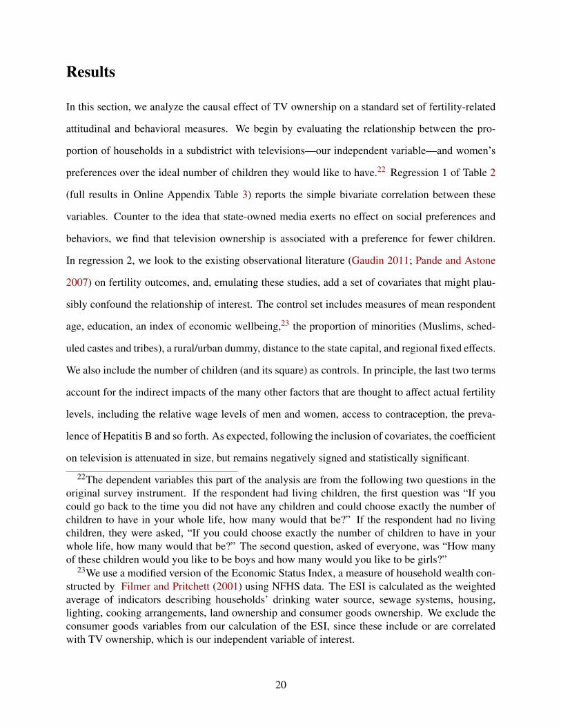
Results

In this section, we analyze the causal effect of TV ownership on a standard set of fertility-related

attitudinal and behavioral measures. We begin by evaluating the relationship between the pro-

portion of households in a subdistrict with televisions—our independent variable—and women’s

preferences over the ideal number of children they would like to have.22 Regression 1 of Table 2

(full results in Online Appendix Table 3) reports the simple bivariate correlation between these

variables. Counter to the idea that state-owned media exerts no effect on social preferences and

behaviors, we find that television ownership is associated with a preference for fewer children.

In regression 2, we look to the existing observational literature (Gaudin 2011; Pande and Astone

2007) on fertility outcomes, and, emulating these studies, add a set of covariates that might plau-

sibly confound the relationship of interest. The control set includes measures of mean respondent

age, education, an index of economic wellbeing,23 the proportion of minorities (Muslims, sched-

uled castes and tribes), a rural/urban dummy, distance to the state capital, and regional fixed effects.

We also include the number of children (and its square) as controls. In principle, the last two terms

account for the indirect impacts of the many other factors that are thought to affect actual fertility

levels, including the relative wage levels of men and women, access to contraception, the preva-

lence of Hepatitis B and so forth. As expected, following the inclusion of covariates, the coefficient

on television is attenuated in size, but remains negatively signed and statistically significant.

22The dependent variables this part of the analysis are from the following two questions in theoriginal survey instrument. If the respondent had living children, the first question was “If youcould go back to the time you did not have any children and could choose exactly the number ofchildren to have in your whole life, how many would that be?” If the respondent had no livingchildren, they were asked, “If you could choose exactly the number of children to have in yourwhole life, how many would that be?” The second question, asked of everyone, was “How manyof these children would you like to be boys and how many would you like to be girls?”

23We use a modified version of the Economic Status Index, a measure of household wealth con-structed by Filmer and Pritchett (2001) using NFHS data. The ESI is calculated as the weightedaverage of indicators describing households’ drinking water source, sewage systems, housing,lighting, cooking arrangements, land ownership and consumer goods ownership. We exclude theconsumer goods variables from our calculation of the ESI, since these include or are correlatedwith TV ownership, which is our independent variable of interest.

20

[Insert Table 2 about here]

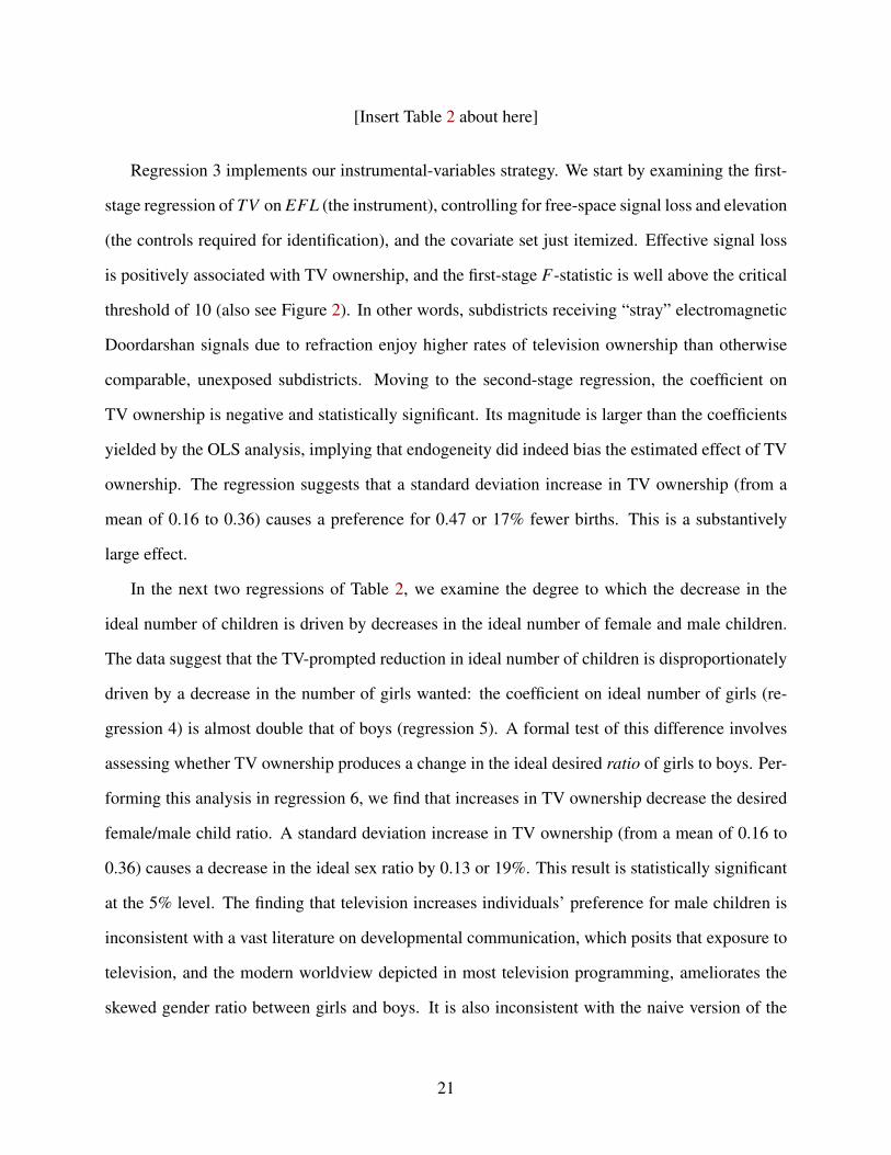
Regression 3 implements our instrumental-variables strategy. We start by examining the first-

stage regression of TV on EFL (the instrument), controlling for free-space signal loss and elevation

(the controls required for identification), and the covariate set just itemized. Effective signal loss

is positively associated with TV ownership, and the first-stage F-statistic is well above the critical

threshold of 10 (also see Figure 2). In other words, subdistricts receiving “stray” electromagnetic

Doordarshan signals due to refraction enjoy higher rates of television ownership than otherwise

comparable, unexposed subdistricts. Moving to the second-stage regression, the coefficient on

TV ownership is negative and statistically significant. Its magnitude is larger than the coefficients

yielded by the OLS analysis, implying that endogeneity did indeed bias the estimated effect of TV

ownership. The regression suggests that a standard deviation increase in TV ownership (from a

mean of 0.16 to 0.36) causes a preference for 0.47 or 17% fewer births. This is a substantively

large effect.

In the next two regressions of Table 2, we examine the degree to which the decrease in the

ideal number of children is driven by decreases in the ideal number of female and male children.

The data suggest that the TV-prompted reduction in ideal number of children is disproportionately

driven by a decrease in the number of girls wanted: the coefficient on ideal number of girls (re-

gression 4) is almost double that of boys (regression 5). A formal test of this difference involves

assessing whether TV ownership produces a change in the ideal desired ratio of girls to boys. Per-

forming this analysis in regression 6, we find that increases in TV ownership decrease the desired

female/male child ratio. A standard deviation increase in TV ownership (from a mean of 0.16 to

0.36) causes a decrease in the ideal sex ratio by 0.13 or 19%. This result is statistically significant

at the 5% level. The finding that television increases individuals’ preference for male children is

inconsistent with a vast literature on developmental communication, which posits that exposure to

television, and the modern worldview depicted in most television programming, ameliorates the

skewed gender ratio between girls and boys. It is also inconsistent with the naive version of the

21

modernization hypothesis, which posits “all good things go together” (Huntington 1968, 5).24

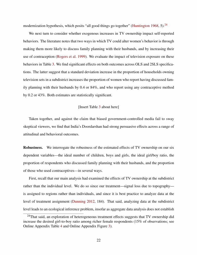
We next turn to consider whether exogenous increases in TV ownership impact self-reported

behaviors. The literature notes that two ways in which TV could alter women’s behavior is through

making them more likely to discuss family planning with their husbands, and by increasing their

use of contraception (Rogers et al. 1999). We evaluate the impact of television exposure on these

behaviors in Table 3. We find significant effects on both outcomes across OLS and 2SLS specifica-

tions. The latter suggest that a standard deviation increase in the proportion of households owning

television sets in a subdistrict increases the proportion of women who report having discussed fam-

ily planning with their husbands by 0.4 or 84%, and who report using any contraceptive method

by 0.2 or 43%. Both estimates are statistically significant.

[Insert Table 3 about here]

Taken together, and against the claim that biased government-controlled media fail to sway

skeptical viewers, we find that India’s Doordarshan had strong persuasive effects across a range of

attitudinal and behavioral outcomes.

Robustness. We interrogate the robustness of the estimated effects of TV ownership on our six

dependent variables—the ideal number of children, boys and girls, the ideal girl/boy ratio, the

proportion of respondents who discussed family planning with their husbands, and the proportion

of those who used contraceptives—in several ways.

First, recall that our main analysis had examined the effects of TV ownership at the subdistrict

rather than the individual level. We do so since our treatment—signal loss due to topography—

is assigned to regions rather than individuals, and since it is best practice to analyze data at the

level of treatment assignment (Dunning 2012, 184). That said, analyzing data at the subdistrict

level leads to an ecological inference problem, insofar as aggregate data analysis does not establish

24That said, an exploration of heterogeneous treatment effects suggests that TV ownership didincrease the desired girl-to-boy ratio among richer female respondents (15% of observations; seeOnline Appendix Table 4 and Online Appendix Figure 3).

22

whether those with TVs in their households are themselves affected by the treatment. We therefore

re-run the regressions using individual-level data, clustering standard errors by subdistrict (the unit

at which we calculate signal losses). Our results are fully robust to this change in the level of

analysis (see Online Appendix Table 6).

Second, Online Appendix Table 7 shows that the main findings remain essentially unaltered

after incorporating survey weights (regressions 1–6), which allow us to assess the effects of TV in

India as a whole. Lastly, the table also shows that the results remain robust to taking the natural

log of the ideal number of children, boys and girls (regressions 7–9), which might be a more

appropriate functional form for these dependent variables.

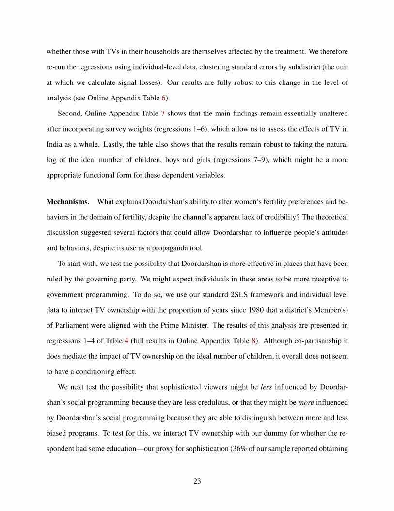
Mechanisms. What explains Doordarshan’s ability to alter women’s fertility preferences and be-

haviors in the domain of fertility, despite the channel’s apparent lack of credibility? The theoretical

discussion suggested several factors that could allow Doordarshan to influence people’s attitudes

and behaviors, despite its use as a propaganda tool.

To start with, we test the possibility that Doordarshan is more effective in places that have been

ruled by the governing party. We might expect individuals in these areas to be more receptive to

government programming. To do so, we use our standard 2SLS framework and individual level

data to interact TV ownership with the proportion of years since 1980 that a district’s Member(s)

of Parliament were aligned with the Prime Minister. The results of this analysis are presented in

regressions 1–4 of Table 4 (full results in Online Appendix Table 8). Although co-partisanship it

does mediate the impact of TV ownership on the ideal number of children, it overall does not seem

to have a conditioning effect.

We next test the possibility that sophisticated viewers might be less influenced by Doordar-

shan’s social programming because they are less credulous, or that they might be more influenced

by Doordarshan’s social programming because they are able to distinguish between more and less

biased programs. To test for this, we interact TV ownership with our dummy for whether the re-

spondent had some education—our proxy for sophistication (36% of our sample reported obtaining

23

some schooling; see regressions 5–8 of Table 4; full results in Online Appendix Table 9). The in-

teraction of the dummy for schooling and TV ownership is negative and statistically significant

on the dependent variables for discussing family planning and contraceptive use, suggesting that

educated viewers are less likely to be swayed by TV with regard to these outcomes.

Were Doordarshan’s explicit or implicit messaging campaigns more effective with regards to

fertility? Here, we leverage the fact that the NFHS asked respondents whether they had heard

a family planning message on TV in the past month. OLS is employed for this analysis (2SLS

is no longer possible, since we have one instrumental variable, and two endogenous independent

variables). These results ought be interpreted with caution due to endogeneity concerns, and thus

we only discuss the relative rather than the absolute magnitudes of the regression coefficients. Al-

though both TV ownership and exposure to family planning messages are separately associated

with a desire for fewer children (regressions 1 and 2 of Table 5), once both variables are included

in the model (regression 3), the magnitude and significance of TV ownership—now a proxy for

general programming—diminishes, whereas the coefficient on family planning messages remains

substantively and statistically significant. This indicates that Doordarshan’s explicit family plan-

ning messages may have played an important role in reducing ideal family sizes. The same is true

with regards to the proportion of women who discuss family planning with their husbands (re-

gression 4). Lastly, a similar analysis with the proportion of respondents that used contraception

specified as the dependent variable suggests that both explicit and implicit messaging increased

contraceptive use.25 Overall, these results suggest that explicit family planning messages worked

better than implicit ones.

[Insert Table 5 about here]

Perhaps our most puzzling result is the unexpected decrease in the desired girl/boy ratio. We

advance two possible mechanisms by which this might obtain. First, the increase in son preference

25Regrettably, we are unable to carry out a parallel analysis for son preference, since the NFHSsurvey did not ask women about their exposure to public service messages discouraging sex selec-tion and advocating gender equality.

24

might be symptomatic of an “intensification” of son preference caused by the reduction in the

number of desired children. In many contexts, including China and parts of sub-Saharan Africa,

women are thought to have a strong preference to give birth to at least one son. In India, this

preference might stem from the Hindu requirement that male heirs perform funeral rights (Arnold,

Choe and Roy 1998), as well as patrilineal inheritance rules (Dyson and Moore 1983). Assume

that for any one pregnancy the probability of giving birth to a boy is 0.5 (in fact it is somewhat

higher). For a woman wishing to give birth to 5 children, the probability of not having a single

boy is (0.5)5, a negligible 0.03125. Yet, as the total number of children desired goes down, the

probability of not producing a single son increases exponentially: it is 0.0625 for 4 children, 0.125

for 3 children, 0.25 for 2 children, and, of course, 0.5 for one child. All else equal, therefore, a

decrease in ideal family size could lead to an intensification in a woman’s desire that her next child

be a son.26 While intuitively appealing, fully validating the operation of the intensification effect

would require experimentally manipulating the hypothetical number of children without changing

son preference (see Jayachandran 2014 for an exercise along these lines), which is an exercise

beyond the scope of this paper.27

Second, we argue that Doordarshan’s depiction of modern urban lifestyles may have inadver-

tently increased son preference by raising the price of girls relative to boys. In particular, we

argue that Doordarshan increased consumerism, which increased the cost of raising girls relative

to boys given the institution of dowry and the practice of women moving to their in-laws’ home,

26A number of other studies have posited the existence of an “intensification” effect, along theseexact lines. Some have found supporting evidence (Basu 2000; Jayachandran 2014), while othershave disputed it (Dreze and Murthi 2001; Klasen 2008).

27That said, we have prima facie reasons to doubt that the decrease in the desired number ofchildren explains the decrease in the ideal girl/boy ratio that we observe. First, the negative effectof instrumented TV ownership on the ideal girl/boy ratio survives controlling for the ideal numberof children that a family desires (regression 2 of Online Appendix Table 11). Since the the idealnumber of children is an obvious post-treatment variable, we improve upon this research designby calculating the “controlled direct effect” of TV on the desired sex ratio while holding the idealnumber of children constant (Acharya, Blackwell and Sen Forthcoming; Vansteelandt 2009). Theresults of this so-called sequential g-estimation (Online Appendix Table 11, regression 3) suggestthat TV mainly affects the desired ratio through means other than the effect of TV on the desirednumber of children.

25

and thereby worsened sex selection.

Considerable evidence suggests that TV encouraged consumerism in India. For example,

Mankekar (1999) draws on fieldwork conducted with lower- and middle-class women in north-

ern India between 1990 and 1992 to argue that television helped promote a consumerist culture.

According to one of Mankekar’s interviewees, “these days people lead more ostentatious lives.

Earlier, people lived more simply. Even if they were rich, they didn’t know where to spend

money. Now, with TV, they know” (87). Another claimed that Doordarshan had promoted “greed”

(laalach) (100). Our data support the idea that TV increased consumerism. Using the same instru-

mental variables framework as our main analysis, we examine whether TV ownership increased

the consumption of two consumer goods that embodied upward mobility in India at this time. In

regressions 6 and 7 of Table 5 we see that a standard deviation increase in TV ownership due to

signal loss causes a 0.8 standard deviation increase in refrigerator ownership and a 0.7 standard de-

viation increase in the ownership of scooters. Admittedly, these are imperfect tests of consumerist

preferences—both because refrigerators and scooters might be thought of as investment goods,

and because we cannot be sure that these purchases were made after TV exposure. Nevertheless,

the data suggest that plausibly exogenous exposure to TV causes respondents to be more likely to

purchase these goods, even after controlling for income.

The increase in consumerism in India generated by exposure to TV could have exacerbated son

preference for reasons we now explain. Parents looking to increase their consumption faced pos-

itive incentives to have sons. Employment in India was—and remains—male-dominated, hence

men were the primary source of household income. Moreover, the tradition of women moving to

their in-laws’ home (susral) immediately following marriage means that male wealth is internal-

ized to the son’s family, whereas daughters’ wealth is lost. Further, the escalating costs of dowries,

which many attributed to consumerism, made having daughters an increasingly expensive propo-

sition. Describing the upcoming marriage of her daughter, one mother commented that “We were

so relieved when they [the groom’s family] didn’t ask for anything. We would have been ruined

if they had” (Mankekar 1999, 87). Dowry demands “evoked a very tangible fear in many of the

26

men and women I worked with, and in fact dominated our discussion about [television] serials”

(125). We corroborate this claim with NFHS data from Bihar, in which average dowry demands

(in Rupee amounts) are strongly correlated with TV ownership (r = .27, p = .003).28 Together,

the evidence suggests that TV has increased consumerism and therefore the relative cost of raising

girls as compared with boys. Sex discrimination could plausibly have resulted from these trends.29

Discussion

Many governments across the world employ public broadcasting as a propaganda tool to boost their

electoral prospects. Partly as a result, popular distrust in state-owned media runs high in numerous

developing nations. Yet, at the same time, governments continue to invest great hopes in state-

run radio and television as instruments of social change. Development communication programs

intended to tackle major development challenges—from improving agricultural productivity, to

mitigating inter-ethnic discord—flood the airwaves in low-income countries. Are these campaigns

successful? Or do citizens disregard instructive messaging that originates from biased official

media outlets? We suggest the latter is not the case. Marshaling evidence from India, we show that

exposure to India’s monopolistic state broadcaster, Doordarshan, had a large, measurable impact on

women’s fertility preferences and behaviors. Doordarshan’s messaging on family planning matters

28The dowry-related questions were only asked in Bihar.29A third means by which Doordarshan’s general programming could have inadvertently wors-

ened son preference is through the transmission of traditional social mores. The producers ofDoordarshan’s serials had to walk a tightrope, between making programs socially progressive,on the one hand, but easily relatable, on the other. To draw audiences, serials incorporated thetropes and conventions characteristic of everyday Indian life. By sometimes reproducing prevail-ing norms, Doordarshan serials may have unwittingly reinforced attitudes about women’s subor-dinate status in family and society, which could have worsened son preference.The extent of thedifficulties in crafting didactic yet popular programming is suggested by the charge that even thepro-development soap, Hum Log, introduced earlier, “reinforces a nostalgia for the benevolent pa-triarchy, order, and harmony supposedly represented by the extended family of the past” (Mankekar1999, 111). Although this is the case, the fact that the TV does not increase son preference amongthe rich (see Online Appendix Table 4 and Online Appendix Figure 3) suggests that TV messagingper se was not the problem.

27

proved persuasive to citizens, despite extensive evidence that a major fraction of Doordarshan

coverage, as well as the station’s rollout, was beset by political interference.

An important contribution of these findings is to provide new, well-identified evidence on a

central tenet of modernization theory: namely, the idea that governments can transform traditional

societies via the media. Recent growth in access to information technology—including television,

smartphones, and the internet—present fresh opportunities for governments to transmit educative

messages to citizens. Encouragingly, our results highlight the force of these communications. But

the substantive findings also sound a warning. In our sample, anti-female bias, which is a seem-

ingly age-old phenomenon, is worsened by the advent of television. We take this as micro-level

evidence for the surprising “modernity of tradition” (Rudolph 1984). In practical terms, govern-

ments looking to impart family planning messages through the media must be careful to counteract

a possibly attendant increase in son preference, perhaps by producing televised messages that more

effectively advance gender equality.

The paper’s findings have implications for two additional areas of active research. We lend

a new perspective to the institutionalist literature on media bias. Studies in this field typically

converge in portraying government-run media in low-income settings as little more than ruling-

party puppets—widely discredited and ignored, and supplying little meaningful content. Yet this

overlooks the parallel, and arguably more significant day-to-day operation of state media as a

source of rich, non-political information for citizens. Addressing when and why governments

enlist the media to pursue developmental, as opposed to purely party-political, ends represents an

important question going forward.

We also contribute to work on the persuasive effects of the media. Our paper extends this line

of inquiry both by investigating the impact of public (rather than private) broadcasting, and by

focusing on a set of social outcomes neglected by political scientists. More deeply, our findings

enrich our understanding of when, and in what areas, partisan or slanted media outlets register

an impact. One interpretation of the results is that citizens in government-controlled media en-

vironments engage in “partitioned viewing:” potentially discounting biased news coverage while

28

retaining interest in non-political programming broadcast on the same channels. This possibility is

consistent with recent work on China and Russia which finds that citizens, though fully cognizant

of state-media biases, continue to express trust in these sources (Mickiewicz 2004; Truex 2016).

Nevertheless, much remains to be determined about the mechanisms by which developmen-

tal media shifts citizen attitudes and behavior. Do campaigns work principally through changing

underlying attitudes, or through knowledge diffusion? To what extent are individuals influenced

through communities and social networks? And do transitions toward greater independence for

state broadcasters amplify the effects of development communications? In examining these top-

ics, researchers should capitalize on new data sources and identification strategies, of the kind

leveraged here.

Before finishing, it is important to consider the generalizability of these findings to countries

beyond India. Demographic control remains a mainstay of government policy the world over,

particularly in developing states. At the London Summit on Family Planning in 2012, for exam-

ple, over 150 country- and donor-leaders pledged to extend access to family planning services to

120 million more women and girls globally. Further, state-owned public service broadcasting is

ubiquitous, and is common to both democracies and non-democratic regimes. It seems quite pos-

sible, therefore, that the results we identify would replicate in other parts of South Asia, China and

Sub-Saharan Africa, which have recently witnessed surges in media penetration and concomitant

changes in fertility.

References

Acharya, Avidit, Matthew Blackwell and Maya Sen. Forthcoming. “Explaining Causal Findings

Without Bias: Detecting and Assessing Direct Effects.” American Political Science Review .

Anderson, Siwan and Debraj Ray. 2010. “Missing Women: Age and Disease.” The Review of

Economic Studies 77(4):1262–1300.

Arceneaux, Kevin, Martin Johnson and Chad Murphy. 2012. “Polarized political communication,

29

oppositional media hostility, and selective exposure.” The Journal of Politics 74(01):174–186.

Arceneaux, Kevin, Martin Johnson and John Cryderman. 2013. “Communication, persuasion, and

the conditioning value of selective exposure: Like minds may unite and divide but they mostly

tune out.” Political communication 30(2):213–231.

Arnold, Fred, Minja Kim Choe and TK Roy. 1998. “Son preference, the family-building process

and child mortality in India.” Population studies 52(3):301–315.

Banerjee, Abhijit and Esther Duflo. 2011. Poor economics: A radical rethinking of the way to fight

global poverty. New York: Public Affairs.

Basu, Alaka. 2000. “Fertility decline and worsening gender bias in India: A response to S. Irudaya

Rajan et al.” Development and Change 31(5):1093–1095.

Besley, Timothy and Andrea Prat. 2006. “Handcuffs for the grabbing hand? The role of the media

in political accountability.” American Economic Review 96(3):720–736.

Bray, Margaret and David M Kreps. 1987. Rational learning and rational expectations. Springer.

Chanda, Ashok. 1966. Radio and Television: Report of the Committee on Broadcasting and Infor-

mation Media. New Delhi: Government of India.

Cleland, John, Stan Bernstein, Alex Ezeh, Anibal Faundes, Anna Glasier and Jolene Innis. 2006.

“Family planning: the unfinished agenda.” The Lancet 368(9549):1810–1827.

Clinton, Joshua D and Ted Enamorado. 2014. “The national news medias effect on Congress: How

Fox News affected elites in Congress.” The Journal of Politics 76(04):928–943.

Datta, Amal. 2007. Effects of Television and the Viewers. New Delhi: Mittal Publications.

DellaVigna, Stefano and Ethan Kaplan. 2007. “The Fox News Effect: Media Bias and Voting.”

The Quarterly Journal of Economics 122(3):1187–1234.

DellaVigna, Stefano and Matthew Gentzkow. 2010. “Persuasion: Empirical Evidence.” Annual

Review of Economics 2(1):643–669.

Djankov, Simeon, Caralee McLiesh, Tatiana Nenova and Andrei Shleifer. 2001. Who owns the

media? Technical report National Bureau of Economic Research.

Dreze, Jean and Mamta Murthi. 2001. “Fertility, Education, and Development: Evidence from

30

India.” Population and development review 27(1):33–63.

Dunning, Thad. 2012. Natural experiments in the social sciences: A design-based approach. New

York: Cambridge University Press.

Durante, Ruben, Paolo Pinotti, Andrea Tesei et al. 2015. The Political Legacy of Entertainment

TV. Technical report.

Dyson, Tim and Mick Moore. 1983. “On kinship structure, female autonomy, and demographic

behavior in India.” Population and development review 9(1):35–60.

Egorov, Georgy, Sergei Guriev and Konstantin Sonin. 2009. “Why resource-poor dictators al-

low freer media: A theory and evidence from panel data.” American political science Review

103(04):645–668.

Enikolopov, Ruben, Maria Petrova and Ekaterina Zhuravskaya. 2011. “Media and Political Per-

suasion: Evidence from Russia.” American Economic Review 101(7):3253–3285.

Filmer, Deon and Lant H. Pritchett. 2001. “Estimating Wealth Effects without Expenditure

Data—or Tears: An Application to Educational Enrollments in States of India.” Demography

38(1):115–132.

Gaudin, Sylvestre. 2011. “Son preference in Indian families: Absolute versus relative wealth

effects.” Demography 48(1):343–370.

Gehlbach, Scott and Konstantin Sonin. 2014. “Government control of the media.” Journal of

Public Economics 118:163–171.

Gentzkow, Matthew. 2006. “Television and voter turnout.” The Quarterly Journal of Economics

pp. 931–972.

Gentzkow, Matthew and Jesse M Shapiro. 2010. “What drives media slant? Evidence from US

daily newspapers.” Econometrica 78(1):35–71.

Gerber, Alan S, James G Gimpel, Donald P Green and Daron R Shaw. 2011. “How large and

long-lasting are the persuasive effects of televised campaign ads? Results from a randomized

field experiment.” American Political Science Review 105(01):135–150.

Ghose, Bhaskar. 2005. Doordarshan days. New Delhi: Penguin, Viking.

31

Government of Rwanda. 2014. “Family Planning in Rwanda: A Review of National and District

Policies and Budgets.” Ministry of Health .

Green, Donald P, Brian R Calfano and Peter M Aronow. 2014. “Field experimental designs for the

study of media effects.” Political Communication 31(1):168–180.

Gunther, Albert C, Cindy T Christen, Janice L Liebhart and Stella Chih-Yun Chia. 2001. “Con-

genial public, contrary press, and biased estimates of the climate of opinion.” Public Opinion

Quarterly 65(3):295–320.

Huber, Gregory A and Kevin Arceneaux. 2007. “Identifying the persuasive effects of presidential

advertising.” American Journal of Political Science 51(4):957–977.

Hufford, G. A. 1995. “The ITS Irregular Terrain Model, version 1.2.2 The Algorithm.”.

Huntington, Samuel P. 1968. Political order in changing societies. Yale University Press.

Jakubowicz, Karol. 1995. “Media within and without the state: Press freedom in Eastern Europe.”

Journal of communication 45(4):125–139.

Jayachandran, Seema. 2014. Fertility Decline and Missing Women. Technical report National

Bureau of Economic Research.

Jeffrey, Robin. 2008. The Mahatma didn’t like the movies and why it matters. In Television in

India: Satellites, Politics and Cultural Change, ed. N. Mehta. London: Routledge.

Jensen, Robert and Emily Oster. 2009. “The Power of TV: Cable Television and Women’s Status

in India.” Quarterly Journal of Economics 124(3):1057–1094.

Johnson, Kirk. 2001. “Media and social change: the modernizing influences of television in rural

India.” Media, Culture & Society 23(2):147–169.

Klasen, Stephan. 2008. Missing women: some recent controversies on levels and trends in gender

bias in mortality. Technical report Ibero America Institute for Economic Research.

Klasen, Stephan and Claudia Wink. 2003. “”Missing women”: Revisiting the debate.” Feminist

Economics 9(2-3):263–299.

La Ferrara, Eliana, Alberto Chong and Suzanne Duryea. 2012. “Soap Operas and Fertility: Evi-

dence from Brazil.” American Economic Journal: Applied Economics 4(4):1–31.

32

Lawson, Chappell H and Sallie Hughes. 2004. “Propaganda and crony capitalism: Partisan bias in

Mexican television news.” Latin American Research Review 39(3):81–105.

Lerner, Daniel. 1958. “The passing of traditional society: Modernizing the Middle East.”.

Lipset, Seymour Martin. 1960. Political Man. The Social Bases of Politics Garden City. Double-

day.

Malik, Saroj. 1989. “Television and rural India.” Media, Culture & Society 11(4):459–484.

Mankekar, Purnima. 1999. Screening culture, viewing politics: An ethnography of television,

womanhood, and nation in postcolonial India. Duke University Press.

Mickiewicz, Ellen. 2004. “Does trustmean attention, comprehension and acceptance?” Mass

media and political communication in new democracies p. 163.

Moehler, Devra C and Naunihal Singh. 2009. “Whose news do you trust? Explaining trust in

private versus public media in Africa.” Political Research Quarterly .

Monteiro, Anjali and KP Jayasankar. 1994. “The spectator-Indian: an exploratory study on the

reception of news.” Cultural studies 8(1):162–182.

Ninan, Sevati. 1992. “DD social service ads preach, but rarely convert.” Down to Earth December

15.

Olken, Benjamin A. 2009. “Do Television and Radio Destroy Social Capital? Evidence from

Indonesian Villages.” American Economic Journal: Applied Economics 1(4):1–33.

Paluck, Elizabeth Levy and Donald P Green. 2009a. “Deference, dissent, and dispute resolution:

An experimental intervention using mass media to change norms and behavior in Rwanda.”

American Political Science Review 103(4):622.

Paluck, Elizabeth Levy and Donald P Green. 2009b. “Prejudice reduction: What works? A review

and assessment of research and practice.” Annual review of psychology 60:339–367.

Pande, Rohini P and Nan Marie Astone. 2007. “Explaining son preference in rural India: the

independent role of structural versus individual factors.” Population Research and Policy Review

26(1):1–29.

Petrova, Maria. 2011. “Newspapers and parties: How advertising revenues created an independent

33

press.” American Political Science Review 105(04):790–808.

Raboy, Marc. 1995. Public broadcasting for the 21st century. Vol. 17 Indiana University Press.

Rao, M. Govinda and Nirvikar Singh. 2001. “The Political Economy of Center-State Fiscal Trans-

fers in India.”.

Rodden, Jonathan and Steven Wilkinson. 2004. “The Shifting Political Economy of Redistribution

in the Indian Federation.”.

Rogers, Everett M, Peter W Vaughan, Ramadhan Swalehe, Nagesh Rao, Peer Svenkerud and Su-

ruchi Sood. 1999. “Effects of an entertainment-education radio soap opera on family planning

behavior in Tanzania.” Studies in family planning 30(3):193–211.

Rudolph, Lloyd I. 1984. The modernity of tradition: Political development in India. University of

Chicago Press.

Rudolph, Lloyd I. 1992. “The media and cultural politics.” Economic and political weekly

pp. 1489–1496.

Ryerson, William N. 1994. “Population communications international: Its role in family planning

soap operas.” Population & Environment 15(4):255–264.

Sen, Amartya. 1990. “More than 100 million women are missing.” The New York Review of Books

37.

Servaes, Jan and Patchanee Malikhao. 2007. “Communication and sustainable development.”

COMMUNICATION AND SUSTAINABLE DEVELOPMENT p. 1.

Singhal, Arvind and Everett M Rogers. 1989. Prosocial television for development in India. New-

bury Park, CA: Sage Publications pp. 331–350.

Singhal, Arvind, Michael J Cody, Everett M Rogers and Miguel Sabido. 2003. Entertainment-

education and social change: History, research, and practice. Routledge.

Srikandath, Sivaram. 1991. “Cultural Values Depicted in Indian Television Advertising.” Interna-

tional Communication Gazette 48(3):165–176.

Stockmann, Daniela and Mary E Gallagher. 2011. “Remote control: How the media sustain au-

thoritarian rule in China.” Comparative Political Studies p. 0010414010394773.

34

Truex, Rory. 2016. “Bias and Trust in Authoritarian Media.”.

Tsfati, Yariv and Gal Ariely. 2013. “Individual and contextual correlates of trust in media across

44 countries.” Communication Research p. 0093650213485972.

Vansteelandt, Stijn. 2009. “Estimating direct effects in cohort and case–control studies.” Epidemi-

ology 20(6):851–860.

World Bank. 2012. World Development Report 2012 : Gender Equality and Development.

Yanigazawa-Drott, David. 2014. “Propaganda and conflict: Theory and evidence from the Rwanda

genocide.” Quarterly Journal of Economics 129(4).

35

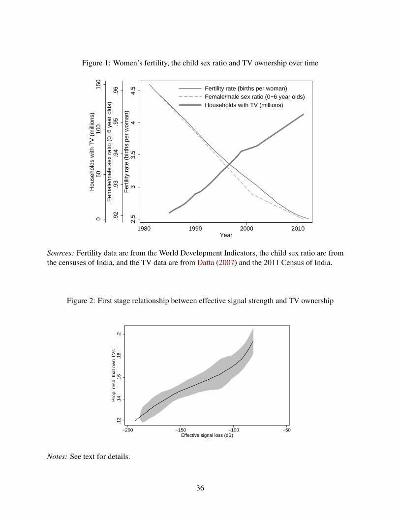
Figure 1: Women’s fertility, the child sex ratio and TV ownership over time

050

100

150

Hou

seho

lds

with

TV

(m

illio

ns)

.92

.93

.94

.95

.96

Fem

ale/

mal

e se

x ra

tio (

0−6

year

old

s)

2.5

33.

54

4.5

Fer

tility

rat

e (b

irths

per

wom

an)

1980 1990 2000 2010Year

Fertility rate (births per woman)Female/male sex ratio (0−6 year olds)Households with TV (millions)

Sources: Fertility data are from the World Development Indicators, the child sex ratio are fromthe censuses of India, and the TV data are from Datta (2007) and the 2011 Census of India.

Figure 2: First stage relationship between effective signal strength and TV ownership

.12

.14

.16

.18

.2P

rop.

res

p. th

at o

wn

TV

s

−200 −150 −100 −50Effective signal loss (dB)

Notes: See text for details.

36

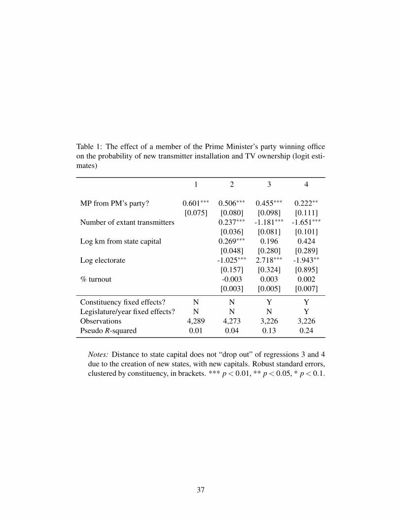
Table 1: The effect of a member of the Prime Minister’s party winning officeon the probability of new transmitter installation and TV ownership (logit esti-mates)

1 2 3 4

MP from PM’s party? 0.601∗∗∗ 0.506∗∗∗ 0.455∗∗∗ 0.222∗∗

[0.075] [0.080] [0.098] [0.111]Number of extant transmitters 0.237∗∗∗ -1.181∗∗∗ -1.651∗∗∗

[0.036] [0.081] [0.101]Log km from state capital 0.269∗∗∗ 0.196 0.424

[0.048] [0.280] [0.289]Log electorate -1.025∗∗∗ 2.718∗∗∗ -1.943∗∗

[0.157] [0.324] [0.895]% turnout -0.003 0.003 0.002

[0.003] [0.005] [0.007]

Constituency fixed effects? N N Y YLegislature/year fixed effects? N N N YObservations 4,289 4,273 3,226 3,226Pseudo R-squared 0.01 0.04 0.13 0.24

Notes: Distance to state capital does not “drop out” of regressions 3 and 4due to the creation of new states, with new capitals. Robust standard errors,clustered by constituency, in brackets. *** p < 0.01, ** p < 0.05, * p < 0.1.

37

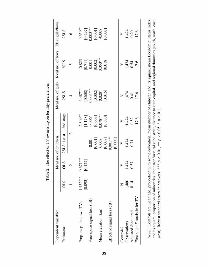
Tabl

e2:

The

effe

ctof

TV

owne

rshi

pon

fert

ility

pref

eren

ces

Dep

ende

ntva

riab

le:

Idea

lno.

ofch

ildre

nId

ealn

o.of

girl

sId

ealn

o.of

boys

Idea

lgir

ls/b

oys

Est

imat

or:

OL

SO

LS

2SL

S:1s

tst.

2nd

stag

e2S

LS

2SL

S2S

LS

12

34

56

Prop

.res

p.th

atow

nT

Vs

-1.4

52∗∗

∗-0

.671

∗∗∗

-2.3

09∗∗

-1.4

87∗∗

-0.8

23-0

.659

∗∗

[0.0

93]

[0.1

22]

[1.1

78]

[0.6

08]

[0.7

11]

[0.2

97]

Free

-spa

cesi

gnal

loss

(dB

)-0

.001

0.00

6∗0.

005∗

∗∗0.

001

0.00

3∗∗∗

[0.0

01]

[0.0

03]

[0.0

02]

[0.0

02]

[0.0

01]

Mea

nel

evat

ion

(km

)0.

008

0.07

8∗∗∗

0.02

8∗0.

050∗

∗∗-0

.008

[0.0

07]

[0.0

30]

[0.0

15]

[0.0

18]

[0.0

08]

Eff

ectiv

esi

gnal

loss

(dB

)0.

001∗

∗∗

[0.0

00]

Con

trol

s?N

YY

YY

YY

Obs

erva

tions

1,48

01,

474

1,47

41,

474

1,47

41,

474

1,47

4A

djus

ted

R-s

quar

ed0.

140.

570.

710.

520.

410.

540.

20Fi

rsts

tage

F-s

tatis

ticfo

rTV

17.6

17.6

17.6

17.6

Not

es:

Con

trol

sar

em

ean

age,

prop

ortio

nw

ithso

me

educ

atio

n,m

ean

num

bero

fchi

ldre

nan

dits

squa

re,m

ean

Eco

nom

icSt

atus

Inde

xan

dits

squa

re,p

ropo

rtio

nof

min

oriti

es,i

ndic

ator

forr

ural

subd

istr

ict,

dist

ance

tost

ate

capi

tal,

and

regi

onal

dum

mie

s(s

outh

,nor

th,e

ast,

wes

t).R

obus

tsta

ndar

der

rors

inbr

acke

ts.*

**p<

0.01

,**

p<

0.05

,*p<

0.1.

38

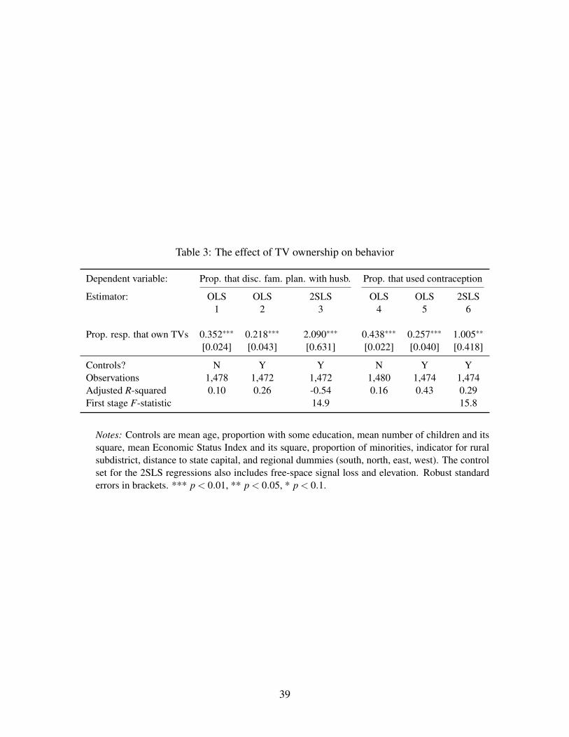
Table 3: The effect of TV ownership on behavior

Dependent variable: Prop. that disc. fam. plan. with husb. Prop. that used contraception

Estimator: OLS OLS 2SLS OLS OLS 2SLS1 2 3 4 5 6

Prop. resp. that own TVs 0.352∗∗∗ 0.218∗∗∗ 2.090∗∗∗ 0.438∗∗∗ 0.257∗∗∗ 1.005∗∗

[0.024] [0.043] [0.631] [0.022] [0.040] [0.418]

Controls? N Y Y N Y YObservations 1,478 1,472 1,472 1,480 1,474 1,474Adjusted R-squared 0.10 0.26 -0.54 0.16 0.43 0.29First stage F-statistic 14.9 15.8

Notes: Controls are mean age, proportion with some education, mean number of children and itssquare, mean Economic Status Index and its square, proportion of minorities, indicator for ruralsubdistrict, distance to state capital, and regional dummies (south, north, east, west). The controlset for the 2SLS regressions also includes free-space signal loss and elevation. Robust standarderrors in brackets. *** p < 0.01, ** p < 0.05, * p < 0.1.

39

Table 4: Mechanisms for the effect of TV—alignment and sophistication

Dependent variable: Ideal no. Ideal girls/ Pr. disc. fam. Pr. usedof children boys plan. with husb. contraception

1 2 3 4

Owns TV -0.010 -0.396∗ 1.408∗∗∗ 0.736∗

[1.397] [0.214] [0.462] [0.392]Owns TV x Degree of alignment with PM -1.545∗ 0.152 -0.097 -0.075

[0.872] [0.104] [0.274] [0.184]Observations 52,200 48,021 31,161 52,200Uncentered R-squared 0.86 0.79 0.33 0.57First stage F-statistic for TV ownership 9.1 12.3 14.4 9.1First stage F-statistic for interaction term 33.9 37.2 39.9 33.9

5 6 7 8

Owns TV -3.073∗∗ -0.374∗ 2.033∗∗∗ 1.237∗∗∗

[1.270] [0.226] [0.531] [0.469]Owns TV x Has schooling 0.595 0.077 -0.791∗∗∗ -0.294∗

[0.409] [0.082] [0.262] [0.153]Observations 54,854 50,356 32,761 54,854Uncentered R-squared 0.80 0.78 0.22 0.45First stage F-statistic for TV ownership 10.4 13.8 11.9 10.4First stage F-statistic for interaction term 76.1 74.2 58.2 76.1

Notes: Controls are mean age, proportion with some education, mean number of children and its square,mean Economic Status Index and its square, proportion of minorities, indicator for rural subdistrict,distance to state capital, regional dummies (south, north, east, west), free-space signal loss and elevation.Regressions 1–4 also control for the proportion of years since 1980 that constituencies’ Members ofParliament(s) were from the party of the Prime Minister. Robust standard errors in brackets, clusteredby subdistrict, in brackets. *** p < 0.01, ** p < 0.05, * p < 0.1.

40

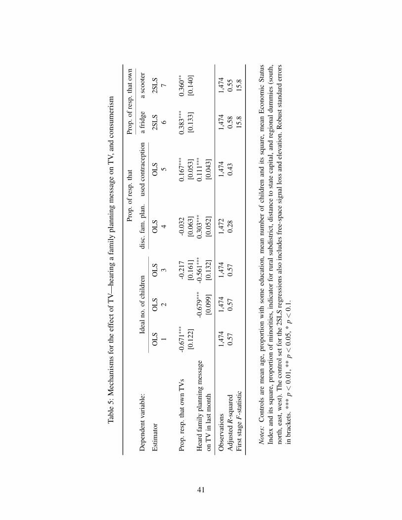
Tabl

e5:

Mec

hani

sms

fort

heef

fect

ofT

V—

hear

ing

afa

mily

plan

ning

mes

sage

onT

V,an

dco

nsum

eris

m

Prop

.ofr

esp.

that

Prop

.ofr

esp.

that

own

Dep

ende

ntva

riab

le:

Idea

lno.

ofch

ildre

ndi

sc.f

am.p

lan.

used

cont

race

ptio

na

frid

gea

scoo

ter

Est

imat

orO

LS

OL

SO

LS

OL

SO

LS

2SL

S2S

LS

12

34

56

7

Prop

.res

p.th

atow

nT

Vs

-0.6

71∗∗

∗-0

.217

-0.0

320.

167∗

∗∗0.

383∗

∗∗0.

360∗

∗

[0.1

22]

[0.1

61]

[0.0

63]

[0.0

53]

[0.1

33]

[0.1

40]

Hea

rdfa

mily

plan

ning

mes

sage

-0.6

79∗∗

∗-0

.561

∗∗∗

0.30

3∗∗∗

0.11

1∗∗∗

onT

Vin

last

mon

th[0

.099

][0

.132

][0

.052

][0

.043

]

Obs

erva

tions

1,47

41,

474

1,47

41,

472

1,47

41,

474

1,47

4A

djus

ted

R-s

quar

ed0.

570.

570.

570.

280.

430.

580.

55Fi

rsts

tage

F-s

tatis

tic15

.815

.8

Not

es:

Con

trol

sar

em

ean

age,

prop

ortio

nw

ithso

me

educ

atio

n,m

ean

num

ber

ofch

ildre

nan

dits

squa

re,

mea

nE

cono

mic

Stat

usIn

dex

and

itssq

uare

,pro

port

ion

ofm

inor

ities

,ind

icat

orfo

rru

rals

ubdi

stri

ct,d

ista

nce

tost

ate

capi

tal,

and

regi

onal

dum

mie

s(s

outh

,no

rth,

east

,wes

t).T

heco

ntro

lset

fort

he2S

LS

regr

essi

ons

also

incl

udes

free

-spa

cesi

gnal

loss

and

elev

atio

n.R

obus

tsta

ndar

der

rors

inbr

acke

ts.*

**p<

0.01

,**

p<

0.05

,*p<

0.1.

41

Online Appendix for “Can Government-ControlledMedia Cause Social Change? Television and Fertility

in India”

Figures

1 A representation of the effect of transmitter attributes on signal reception . . . . . . 2

2 Effective signal loss map . . . . . . . . . . . . . . . . . . . . . . . . . . . . . . . 3

3 Heterogeneous effects of TV ownership on ideal girls/boys . . . . . . . . . . . . . 4

Tables

1 Summary statistics for subdistrict-level fertility dataset . . . . . . . . . . . . . . . 5

2 Balance tests for potential correlates of effective signal loss (OLS) . . . . . . . . . 6

3 The effect of TV ownership on fertility preferences . . . . . . . . . . . . . . . . . 7

4 Heterogeneous effects of TV ownership on ideal girls/boys . . . . . . . . . . . . . 8

5 The effect of TV ownership on behavior . . . . . . . . . . . . . . . . . . . . . . . 9

6 Robustness tests: Individual level analysis . . . . . . . . . . . . . . . . . . . . . . 10

7 Robustness tests: Weighted regressions, natural logged DVs . . . . . . . . . . . . 11

8 Mechanisms for the effect of TV—alignment . . . . . . . . . . . . . . . . . . . . 12

9 Mechanisms for the effect of TV—sophistication . . . . . . . . . . . . . . . . . . 13

10 Mechanisms for the effect of TV—family planning messages, and consumerism . . 14

11 Mechanism for the effect of TV on the ideal girl/boy ratio—intensification . . . . . 15

Dataset construction . . . . . . . . . . . . . . . . . . . . . . . . . . . . . . . . . . . . . . . . . . . . . . . . . . . . . . . . . 17

1

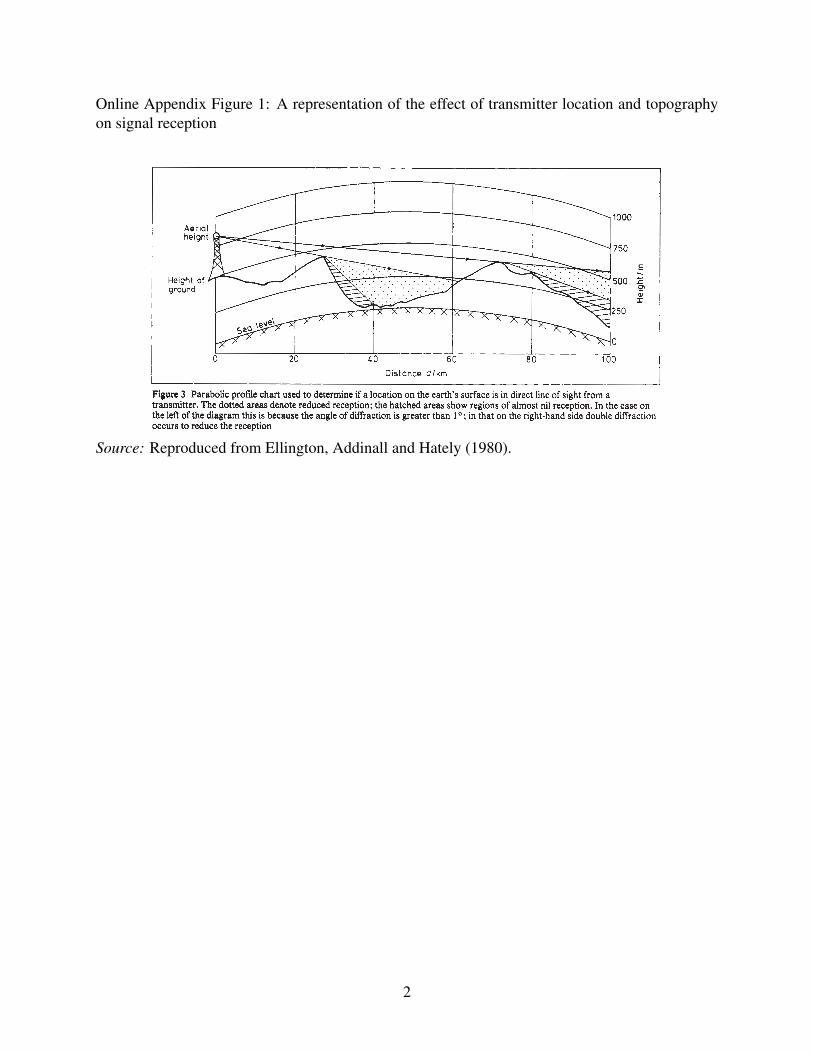
Online Appendix Figure 1: A representation of the effect of transmitter location and topographyon signal reception

Source: Reproduced from Ellington, Addinall and Hately (1980).

2

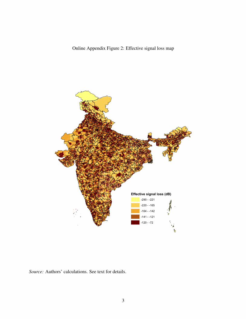
Online Appendix Figure 2: Effective signal loss map

Effective signal loss (dB)

-290 - -221

-220 - -165

-164 - -142

-141 - -121

-120 - -72

Source: Authors’ calculations. See text for details.

3

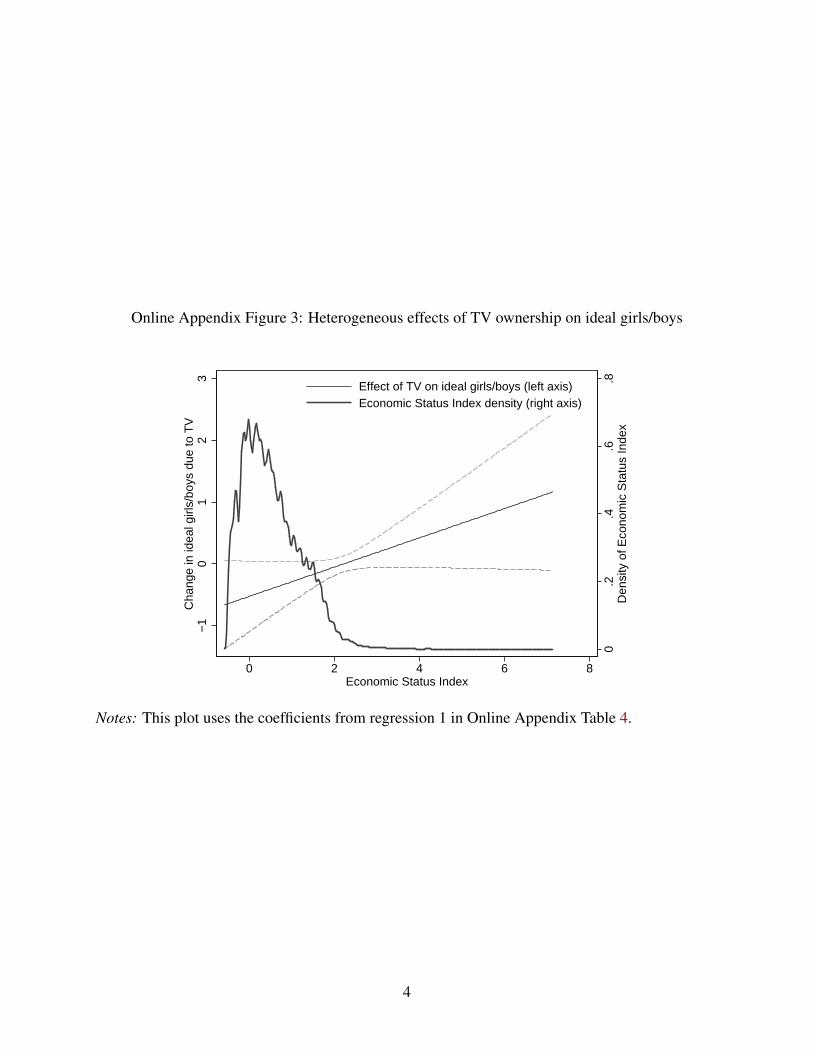
Online Appendix Figure 3: Heterogeneous effects of TV ownership on ideal girls/boys

0.2

.4.6

.8D

ensi

ty o

f Eco

nom

ic S

tatu

s In

dex

−1

01

23

Cha

nge

in id

eal g

irls/

boys

due

to T

V

0 2 4 6 8Economic Status Index

Effect of TV on ideal girls/boys (left axis)Economic Status Index density (right axis)

Notes: This plot uses the coefficients from regression 1 in Online Appendix Table 4.

4

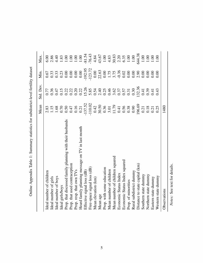
Onl

ine

App

endi

xTa

ble

1:Su

mm

ary

stat

istic

sfo

rsub

dist

rict

-lev

elfe

rtili

tyda

tase

t

Mea

nSt

d.D

ev.

Min

.M

ax.

Idea

lnum

bero

fchi

ldre

n2.

830.

770.

676.

00Id

ealn

umbe

rofg

irls

1.15

0.36

0.33

2.86

Idea

lnum

bero

fboy

s1.

680.

470.

334.

40Id

ealg

irls

/boy

s0.

700.

150.

231.

83Pr

op.t

hatd

iscu

ssed

fam

ilypl

anni

ngw

ithth

eirh

usba

nds

0.50

0.22

0.00

1.00

Prop

.tha

tuse

dco

ntra

cept

ion

0.47

0.22

0.00

1.00

Prop

.res

p.th

atow

nT

Vs

0.16

0.20

0.00

1.00

Hea

rdfa

mily

plan

ning

mes

sage

onT

Vin

last

mon

th0.

210.

220.

001.

00E

ffec

tive

sign

allo

ss(d

B)

-137

.52

15.2

6-1

92.9

5-8

1.54

Free

-spa

cesi

gnal

loss

(dB

)-1

10.0

25.

85-1

23.7

2-7

6.43

Mea

nel

evat

ion

(km

)0.

420.

540.

004.

84M

ean

age

30.5

02.

4022

.63

43.6

7Pr

op.w

ithso

me

educ

atio

n0.

360.

250.

001.

00M

ean

num

bero

fchi

ldre

n3.

010.

461.

754.

83M

ean

num

bero

fchi

ldre

nsq

uare

d11

.79

3.62

3.75

30.8

3E

cono

mic

Stat

usIn

dex

0.41

0.37

-0.3

62.

20E

cono

mic

Stat

usIn

dex

squa

red

0.56

0.57

0.02

6.35

Prop

.ofm

inor

ities

0.38

0.31

0.00

1.00

Rur

alsu

bdis

tric

tdum

my

0.90

0.30

0.00

1.00

Dis

tanc

eto

stat

eca

pita

l(km

)19

6.69

132.

362.

9064

4.38

Sout

hern

stat

edu

mm

y0.

210.

410.

001.

00N

orth

ern

stat

edu

mm

y0.

180.

390.

001.

00E

aste

rnst

ate

dum

my

0.21

0.41

0.00

1.00

Wes

tern

stat

edu

mm

y0.

250.

430.

001.

00

Obs

erva

tions

1480

Not

es:

See

text

ford

etai

ls.

5

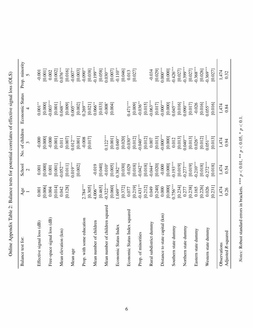
Onl

ine

App

endi

xTa

ble

2:B

alan

cete

sts

forp

oten

tialc

orre

late

sof

effe

ctiv

esi

gnal

loss

(OL

S)

Bal

ance

test

for:

Age

Scho

olN

o.of

child

ren

Eco

nom

icSt

atus

Prop

.min

ority

12

34

5

Eff

ectiv

esi

gnal

loss

(dB

)0.

001

0.00

1-0

.000

0.00

1∗∗

-0.0

01[0

.006

][0

.000

][0

.000

][0

.000

][0

.001

]Fr

ee-s

pace

sign

allo

ss(d

B)

0.00

40.

001

-0.0

00-0

.003

∗∗∗

0.00

2[0

.014

][0

.001

][0

.001

][0

.001

][0

.002

]M

ean

elev

atio

n(k

m)

0.04

2-0

.052

∗∗∗

0.01

10.

048∗

∗∗0.

076∗

∗∗

[0.1

28]

[0.0

11]

[0.0

07]

[0.0

09]

[0.0

16]

Mea

nag

e0.

019∗

∗∗0.

012∗

∗∗0.

005∗

∗∗-0

.007

∗∗

[0.0

02]

[0.0

01]

[0.0

02]

[0.0

03]

Prop

.with

som

eed

ucat

ion

2.78

4∗∗∗

-0.0

080.

269∗

∗∗-0

.090

∗∗

[0.3

05]

[0.0

17]

[0.0

21]

[0.0

38]

Mea

nnu

mbe

rofc

hild

ren

4.00

6∗∗∗

-0.0

190.

066∗

∗-0

.199

∗∗∗

[0.4

65]

[0.0

40]

[0.0

33]

[0.0

58]

Mea

nnu

mbe

rofc

hild

ren

squa

red

-0.3

22∗∗

∗-0

.010

∗0.

122∗

∗∗-0

.008

∗0.

030∗

∗∗

[0.0

60]

[0.0

05]

[0.0

01]

[0.0

04]

[0.0

07]

Eco

nom

icSt

atus

Inde

x1.

049∗

∗∗0.

382∗

∗∗0.

040∗

∗-0

.110

∗∗

[0.3

72]

[0.0

30]

[0.0

20]

[0.0

46]

Eco

nom

icSt

atus

Inde

xsq

uare

d0.

077

-0.0

29-0

.030

∗∗0.

471∗

∗∗0.

013

[0.2

19]

[0.0

18]

[0.0

12]

[0.0

09]

[0.0

27]

Prop

.ofm

inor

ities

-0.4

31∗∗

-0.0

42∗∗

-0.0

40∗∗

∗-0

.036

∗∗

[0.2

12]

[0.0

18]

[0.0

12]

[0.0

15]

Rur

alsu

bdis

tric

tdum

my

0.04

9-0

.044

∗∗0.

007

-0.0

63∗∗

∗-0

.034

[0.2

40]

[0.0

20]

[0.0

13]

[0.0

17]

[0.0

29]

Dis

tanc

eto

stat

eca

pita

l(km

)0.

000

-0.0

00-0

.000

∗∗∗

-0.0

00∗∗

∗0.

000∗

∗∗

[0.0

00]

[0.0

00]

[0.0

00]

[0.0

00]

[0.0

00]

Sout

hern

stat

edu

mm

y0.

756∗

∗∗-0

.193

∗∗∗

0.01

20.

045∗

∗∗-0

.426

∗∗∗

[0.2

34]

[0.0

19]

[0.0

13]

[0.0

16]

[0.0

27]

Nor

ther

nst

ate

dum

my

0.27

7-0

.277

∗∗∗

0.04

0∗∗∗

0.09

0∗∗∗

-0.3

99∗∗

∗

[0.2

38]

[0.0

19]

[0.0

13]

[0.0

17]

[0.0

27]

Eas

tern

stat

edu

mm

y0.

165

-0.2

10∗∗

∗0.

026∗

∗-0

.026

-0.3

68∗∗

∗

[0.2

26]

[0.0

18]

[0.0

12]

[0.0

16]

[0.0

26]

Wes

tern

stat

edu

mm

y0.

026

-0.2

72∗∗

∗0.

051∗

∗∗0.

055∗

∗∗-0

.369

∗∗∗

[0.2

31]

[0.0

18]

[0.0

13]

[0.0

16]

[0.0

27]

Obs

erva

tions

1,47

41,

474

1,47

41,

474

1,47

4A

djus

ted

R-s

quar

ed0.

260.

540.

940.

840.

32

Not

es:

Rob

usts

tand

ard

erro

rsin

brac

kets

.***

p<

0.01

,**

p<

0.05

,*p<

0.1.

6

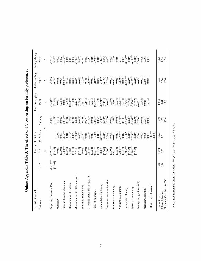
Onl

ine

App

endi

xTa

ble

3:T

heef

fect

ofT

Vow

ners

hip

onfe

rtili

typr

efer

ence

s

Dep

ende

ntva

riab

le:

Idea

lno.

ofch

ildre

nId

ealn

o.of

girl

sId

ealn

o.of

boys

Idea

lgir

ls/b

oys

Est

imat

or:

OL

SO

LS

2SL

S:1s

tst.

2nd

stag

e2S

LS

2SL

S2S

LS

12

34

56

Prop

.res

p.th

atow

nT

Vs

-1.4

52∗∗∗

-0.6

71∗∗∗

-2.3

09∗∗

-1.4

87∗∗

-0.8

23-0

.659

∗∗

[0.0

93]

[0.1

22]

[1.1

78]

[0.6

08]

[0.7

11]

[0.2

97]

Mea

nag

e-0

.010

-0.0

01-0

.012

∗-0

.004

-0.0

08∗

0.00

2[0

.006

][0

.001

][0

.007

][0

.004

][0

.004

][0

.002

]Pr

op.w

ithso

me

educ

atio

n-0

.868

∗∗∗

0.13

5∗∗∗

-0.6

12∗∗∗

-0.0

30-0

.583

∗∗∗

0.23

5∗∗∗

[0.0

78]

[0.0

16]

[0.1

81]

[0.0

93]

[0.1

09]

[0.0

46]

Mea

nnu

mbe

rofc

hild

ren

0.18

30.

046∗

0.24

2∗0.

211∗

∗∗0.

032

0.04

8[0

.117

][0

.025

][0

.134

][0

.069

][0

.081

][0

.034

]M

ean

num

bero

fchi

ldre

nsq

uare

d0.

011

-0.0

08∗∗

0.00

2-0

.015

0.01

7-0

.009

∗∗

[0.0

15]

[0.0

03]

[0.0

18]

[0.0

09]

[0.0

11]

[0.0

05]

Eco

nom

icSt

atus

Inde

x-0

.058

0.21

4∗∗∗

0.26

80.

288∗

∗-0

.020

0.15

6∗∗

[0.0

94]

[0.0

19]

[0.2

74]

[0.1

41]

[0.1

65]

[0.0

69]

Eco

nom

icSt

atus

Inde

xsq

uare

d0.

110∗

∗0.

020∗

0.14

2∗∗

0.03

30.

110∗

∗∗-0

.001

[0.0

54]

[0.0

11]

[0.0

61]

[0.0

31]

[0.0

37]

[0.0

15]

Prop

.ofm

inor

ities

0.52

7∗∗∗

-0.0

090.

483∗

∗∗0.

315∗

∗∗0.

169∗

∗∗0.

098∗

∗∗

[0.0

52]

[0.0

11]

[0.0

56]

[0.0

29]

[0.0

34]

[0.0

14]

Rur

alsu

bdis

tric

tdum

my

-0.0

82-0

.206

∗∗∗

-0.4

07-0

.271

∗∗-0

.137

-0.1

42∗∗

[0.0

61]

[0.0

12]

[0.2

55]

[0.1

31]

[0.1

54]

[0.0

64]

Dis

tanc

eto

stat

eca

pita

l(km

)0.

000

-0.0

00∗∗

-0.0

00-0

.000

-0.0

000.

000

[0.0

00]

[0.0

00]

[0.0

00]

[0.0

00]

[0.0

00]

[0.0

00]

Sout

hern

stat

edu

mm

y-1

.151

∗∗∗

-0.0

35∗∗∗

-1.1

61∗∗∗

-0.5

30∗∗∗

-0.6

30∗∗∗

-0.0

19[0

.056

][0

.012

][0

.071

][0

.037

][0

.043

][0

.018

]N

orth

ern

stat

edu

mm

y-0

.683

∗∗∗

0.09

9∗∗∗

-0.4

74∗∗∗

-0.3

05∗∗∗

-0.1

70∗∗

-0.0

78∗∗

[0.0

58]

[0.0

12]

[0.1

43]

[0.0

74]

[0.0

86]

[0.0

36]

Eas

tern

stat

edu

mm

y-0

.606

∗∗∗

-0.0

02-0

.552

∗∗∗

-0.3

43∗∗∗

-0.2

09∗∗∗

-0.1

04∗∗∗

[0.0

52]

[0.0

12]

[0.0

58]

[0.0

30]

[0.0

35]

[0.0

15]

Wes

tern

stat

edu

mm

y-0

.802

∗∗∗

0.03

3∗∗∗

-0.6

98∗∗∗

-0.4

26∗∗∗

-0.2

73∗∗∗

-0.1

26∗∗∗

[0.0

55]

[0.0

12]

[0.0

72]

[0.0

37]

[0.0

43]

[0.0

18]

Free

-spa

cesi

gnal

loss

(dB

)-0

.001

0.00

6∗0.

005∗

∗∗0.

001

0.00

3∗∗∗

[0.0

01]

[0.0

03]

[0.0

02]

[0.0

02]

[0.0

01]

Mea

nel

evat

ion

(km

)0.

008

0.07

8∗∗∗

0.02

8∗0.

050∗

∗∗-0

.008

[0.0

07]

[0.0

30]

[0.0

15]

[0.0

18]

[0.0

08]

Eff

ectiv

esi

gnal

loss

(dB

)0.

001∗

∗∗

[0.0

00]

Obs

erva

tions

1,48

01,

474

1,47

41,

474

1,47

41,

474

1,47

4A

djus

ted

R-s

quar

ed0.

140.

570.

710.

520.

410.

540.

20Fi

rsts

tage

F-s

tatis

ticfo

rTV

17.6

17.6

17.6

17.6

Not

es:

Rob

usts

tand

ard

erro

rsin

brac

kets

.***

p<

0.01

,**

p<

0.05

,*p<

0.1.

7

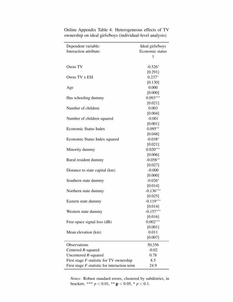
Online Appendix Table 4: Heterogeneous effects of TVownership on ideal girls/boys (individual-level analysis)

Dependent variable: Ideal girls/boysInteraction attribute: Economic status

1

Owns TV -0.526∗

[0.291]Owns TV x ESI 0.237∗

[0.130]Age 0.000

[0.000]Has schooling dummy 0.093∗∗∗

[0.021]Number of children 0.003

[0.004]Number of children squared -0.001

[0.001]Economic Status Index 0.095∗∗

[0.048]Economic Status Index squared -0.038∗

[0.021]Minority dummy 0.020∗∗∗

[0.006]Rural resident dummy -0.058∗∗

[0.027]Distance to state capital (km) -0.000

[0.000]Southern state dummy -0.026∗

[0.014]Northern state dummy -0.136∗∗∗

[0.025]Eastern state dummy -0.119∗∗∗

[0.014]Western state dummy -0.157∗∗∗

[0.016]Free-space signal loss (dB) 0.002∗∗∗

[0.001]Mean elevation (km) 0.011

[0.007]

Observations 50,356Centered R-squared -0.02Uncentered R-squared 0.78First stage F-statistic for TV ownership 8.5First stage F-statistic for interaction term 24.9

Notes: Robust standard errors, clustered by subdistrict, inbrackets. *** p < 0.01, ** p < 0.05, * p < 0.1.8

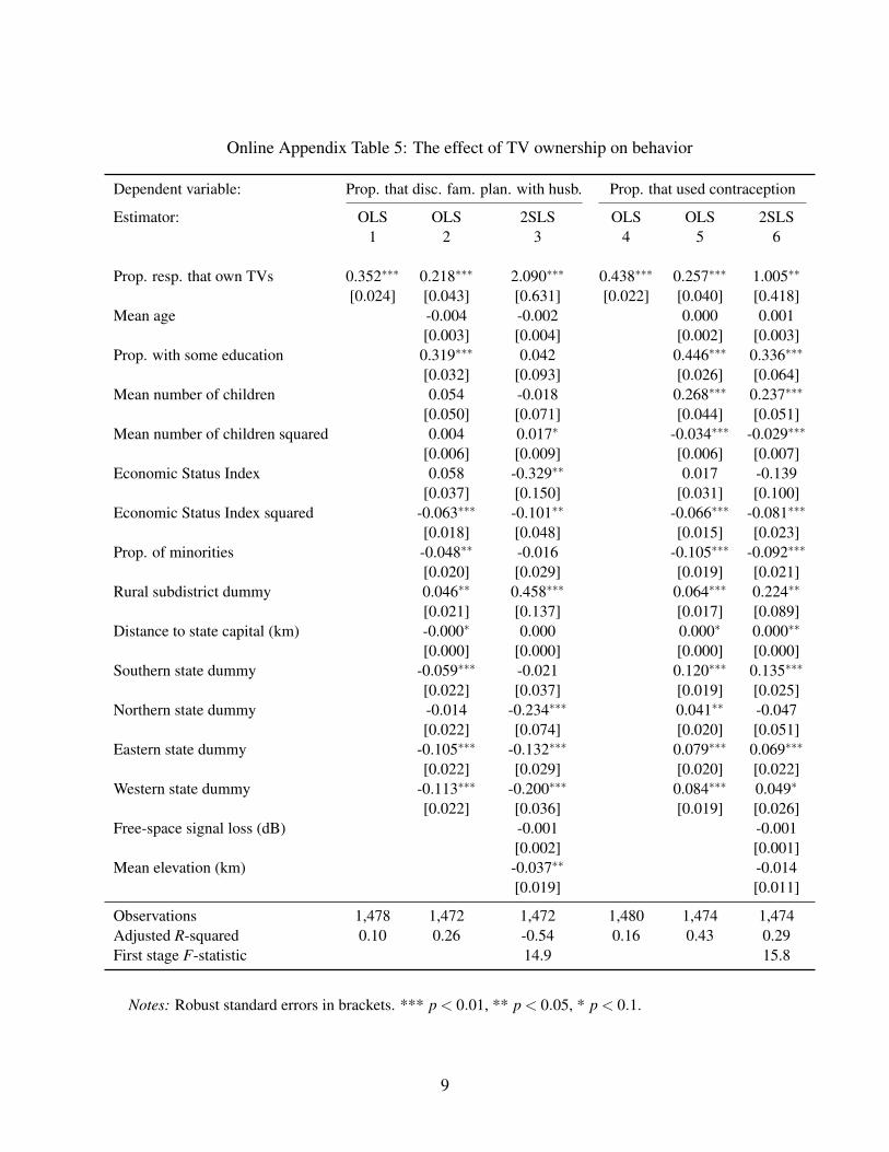
Online Appendix Table 5: The effect of TV ownership on behavior

Dependent variable: Prop. that disc. fam. plan. with husb. Prop. that used contraception

Estimator: OLS OLS 2SLS OLS OLS 2SLS1 2 3 4 5 6

Prop. resp. that own TVs 0.352∗∗∗ 0.218∗∗∗ 2.090∗∗∗ 0.438∗∗∗ 0.257∗∗∗ 1.005∗∗

[0.024] [0.043] [0.631] [0.022] [0.040] [0.418]Mean age -0.004 -0.002 0.000 0.001

[0.003] [0.004] [0.002] [0.003]Prop. with some education 0.319∗∗∗ 0.042 0.446∗∗∗ 0.336∗∗∗

[0.032] [0.093] [0.026] [0.064]Mean number of children 0.054 -0.018 0.268∗∗∗ 0.237∗∗∗

[0.050] [0.071] [0.044] [0.051]Mean number of children squared 0.004 0.017∗ -0.034∗∗∗ -0.029∗∗∗

[0.006] [0.009] [0.006] [0.007]Economic Status Index 0.058 -0.329∗∗ 0.017 -0.139

[0.037] [0.150] [0.031] [0.100]Economic Status Index squared -0.063∗∗∗ -0.101∗∗ -0.066∗∗∗ -0.081∗∗∗

[0.018] [0.048] [0.015] [0.023]Prop. of minorities -0.048∗∗ -0.016 -0.105∗∗∗ -0.092∗∗∗

[0.020] [0.029] [0.019] [0.021]Rural subdistrict dummy 0.046∗∗ 0.458∗∗∗ 0.064∗∗∗ 0.224∗∗

[0.021] [0.137] [0.017] [0.089]Distance to state capital (km) -0.000∗ 0.000 0.000∗ 0.000∗∗

[0.000] [0.000] [0.000] [0.000]Southern state dummy -0.059∗∗∗ -0.021 0.120∗∗∗ 0.135∗∗∗

[0.022] [0.037] [0.019] [0.025]Northern state dummy -0.014 -0.234∗∗∗ 0.041∗∗ -0.047

[0.022] [0.074] [0.020] [0.051]Eastern state dummy -0.105∗∗∗ -0.132∗∗∗ 0.079∗∗∗ 0.069∗∗∗

[0.022] [0.029] [0.020] [0.022]Western state dummy -0.113∗∗∗ -0.200∗∗∗ 0.084∗∗∗ 0.049∗

[0.022] [0.036] [0.019] [0.026]Free-space signal loss (dB) -0.001 -0.001

[0.002] [0.001]Mean elevation (km) -0.037∗∗ -0.014

[0.019] [0.011]

Observations 1,478 1,472 1,472 1,480 1,474 1,474Adjusted R-squared 0.10 0.26 -0.54 0.16 0.43 0.29First stage F-statistic 14.9 15.8

Notes: Robust standard errors in brackets. *** p < 0.01, ** p < 0.05, * p < 0.1.

9

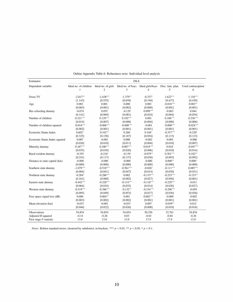
Online Appendix Table 6: Robustness tests: Individual level analysis

Estimator: 2SLS

Dependent variable: Ideal no. of children Ideal no. of girls Ideal no. of boys Ideal girls/boys Disc. fam. plan. Used contraception1 2 3 4 5 6

Owns TV -2.817∗∗ -1.438∗∗∗ -1.379∗∗ -0.337∗ 1.622∗∗∗ 1.110∗∗∗

[1.143] [0.555] [0.658] [0.194] [0.437] [0.430]Age 0.001 0.001 0.000 0.001 -0.016∗∗∗ 0.003∗∗

[0.003] [0.001] [0.002] [0.000] [0.001] [0.001]Has schooling dummy -0.074 0.055 -0.129 0.099∗∗∗ -0.063 0.044

[0.141] [0.069] [0.081] [0.024] [0.064] [0.054]Number of children 0.321∗∗∗ 0.129∗∗∗ 0.192∗∗∗ 0.001 0.106∗∗∗ 0.236∗∗∗

[0.014] [0.007] [0.008] [0.004] [0.008] [0.006]Number of children squared -0.014∗∗∗ -0.006∗∗∗ -0.008∗∗∗ -0.001 -0.008∗∗∗ -0.024∗∗∗

[0.002] [0.001] [0.001] [0.001] [0.001] [0.001]Economic Status Index 0.602∗ 0.342∗∗ 0.260 0.104∗ -0.357∗∗∗ -0.220∗

[0.325] [0.158] [0.187] [0.054] [0.115] [0.123]Economic Status Index squared 0.007 -0.001 0.008 -0.002 -0.001 -0.006

[0.020] [0.010] [0.011] [0.004] [0.010] [0.007]Minority dummy 0.187∗∗∗ 0.100∗∗∗ 0.087∗∗∗ 0.019∗∗∗ 0.010 -0.047∗∗∗

[0.035] [0.018] [0.020] [0.006] [0.018] [0.014]Rural resident dummy -0.355 -0.216∗ -0.139 -0.079∗∗ 0.301∗∗∗ 0.182∗∗

[0.241] [0.117] [0.137] [0.038] [0.093] [0.092]Distance to state capital (km) -0.000 -0.000 -0.000 -0.000 0.000∗∗ 0.000∗

[0.000] [0.000] [0.000] [0.000] [0.000] [0.000]Southern state dummy -1.079∗∗∗ -0.518∗∗∗ -0.561∗∗∗ -0.026∗ -0.111∗∗∗ 0.085∗∗∗

[0.084] [0.041] [0.047] [0.014] [0.030] [0.031]Northern state dummy -0.284∗ -0.286∗∗∗ 0.002 -0.133∗∗∗ -0.253∗∗∗ -0.153∗∗

[0.161] [0.080] [0.092] [0.027] [0.056] [0.061]Eastern state dummy -0.442∗∗∗ -0.328∗∗∗ -0.114∗∗∗ -0.118∗∗∗ -0.229∗∗∗ -0.011

[0.064] [0.034] [0.035] [0.014] [0.026] [0.027]Western state dummy -0.519∗∗∗ -0.386∗∗∗ -0.132∗∗ -0.154∗∗∗ -0.296∗∗∗ -0.059

[0.095] [0.049] [0.053] [0.017] [0.036] [0.036]Free-space signal loss (dB) 0.006 0.004∗∗ 0.001 0.002∗∗∗ -0.000 -0.002

[0.003] [0.002] [0.002] [0.001] [0.001] [0.001]Mean elevation (km) -0.033 -0.001 -0.033 0.007 -0.039∗∗ 0.012

[0.046] [0.022] [0.026] [0.008] [0.018] [0.016]

Observations 54,854 54,854 54,854 50,356 32,761 54,854Adjusted R-squared -0.14 -0.26 0.03 -0.03 -0.84 -0.26First stage F-statistic 13.0 13.0 13.0 17.9 17.9 13.0

Notes: Robust standard errors, clustered by subdistrict, in brackets. *** p < 0.01, ** p < 0.05, * p < 0.1.

10

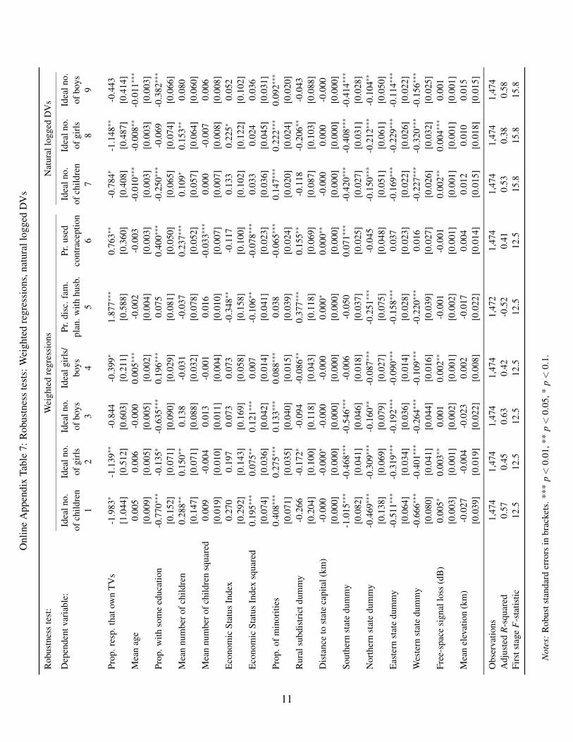
Onl

ine

App

endi

xTa

ble

7:R

obus

tnes

ste

sts:

Wei

ghte

dre

gres

sion

s,na

tura

llog

ged

DV

s

Rob

ustn

ess

test

:W

eigh

ted

regr

essi

ons

Nat

ural

logg

edD

Vs

Dep

ende

ntva

riab

le:

Idea

lno.

Idea

lno.

Idea

lno.

Idea

lgir

ls/

Pr.d

isc.

fam

.Pr

.use

dId

ealn

o.Id

ealn

o.Id

ealn

o.of

child

ren

ofgi

rls

ofbo

ysbo

yspl

an.w

ithhu

sb.

cont

race

ptio

nof

child

ren

ofgi

rls

ofbo

ys1

23

45

67

89

Prop

.res

p.th

atow

nT

Vs

-1.9

83∗

-1.1

39∗∗

-0.8

44-0

.399

∗1.

877∗

∗∗0.

763∗

∗-0

.784

∗-1

.148

∗∗-0

.443

[1.0

44]

[0.5

12]

[0.6

03]

[0.2

11]

[0.5

88]

[0.3

60]

[0.4

08]

[0.4

87]

[0.4

14]

Mea

nag

e0.

005

0.00

6-0

.000

0.00

5∗∗∗

-0.0

02-0

.003

-0.0

10∗∗∗

-0.0

08∗∗

-0.0

11∗∗∗

[0.0

09]

[0.0

05]

[0.0

05]

[0.0

02]

[0.0

04]

[0.0

03]

[0.0

03]

[0.0

03]

[0.0

03]

Prop

.with

som

eed

ucat

ion

-0.7

70∗∗∗

-0.1

35∗

-0.6

35∗∗∗

0.19

6∗∗∗

0.07

50.

400∗

∗∗-0

.250

∗∗∗

-0.0

69-0

.382

∗∗∗

[0.1

52]

[0.0

71]

[0.0

90]

[0.0

29]

[0.0

81]

[0.0

50]

[0.0

65]

[0.0

74]

[0.0

66]

Mea

nnu

mbe

rofc

hild

ren

0.28

8∗∗

0.15

0∗∗

0.13

8-0

.031

-0.0

370.

237∗

∗∗0.

109∗

0.15

3∗∗

0.08

0[0

.147

][0

.071

][0

.088

][0

.032

][0

.078

][0

.052

][0

.057

][0

.064

][0

.060

]M

ean

num

bero

fchi

ldre

nsq

uare

d0.

009

-0.0

040.

013

-0.0

010.

016

-0.0

33∗∗∗

0.00

0-0

.007

0.00

6[0

.019

][0

.010

][0

.011

][0

.004

][0

.010

][0

.007

][0

.007

][0

.008

][0

.008

]E

cono

mic

Stat

usIn

dex

0.27

00.

197

0.07

30.

073

-0.3

48∗∗

-0.1

170.

133

0.22

5∗0.

052

[0.2

92]

[0.1

43]

[0.1

69]

[0.0

58]

[0.1

58]

[0.1

00]

[0.1

02]

[0.1

22]

[0.1

02]

Eco

nom

icSt

atus

Inde

xsq

uare

d0.

195∗

∗∗0.

075∗

∗0.

121∗

∗∗0.

007

-0.1

06∗∗

-0.0

78∗∗∗

0.03

30.

024

0.03

6[0

.074

][0

.036

][0

.042

][0

.014

][0

.041

][0

.023

][0

.036

][0

.045

][0

.031

]Pr

op.o

fmin

oriti

es0.

408∗

∗∗0.

275∗

∗∗0.

133∗

∗∗0.

088∗

∗∗0.

038

-0.0

65∗∗∗

0.14

7∗∗∗

0.22

2∗∗∗

0.09

2∗∗∗

[0.0

71]

[0.0

35]

[0.0

40]

[0.0

15]

[0.0

39]

[0.0

24]

[0.0

20]

[0.0

24]

[0.0

20]

Rur

alsu

bdis

tric

tdum

my

-0.2

66-0

.172

∗-0

.094

-0.0

86∗∗

0.37

7∗∗∗

0.15

5∗∗

-0.1

18-0

.206

∗∗-0

.043

[0.2

04]

[0.1

00]

[0.1

18]

[0.0

43]

[0.1

18]

[0.0

69]

[0.0

87]

[0.1

03]

[0.0

88]

Dis

tanc

eto

stat

eca

pita

l(km

)-0

.000

-0.0

00∗

-0.0

00-0

.000

0.00

0∗0.

000∗

∗-0

.000

0.00

0-0

.000

[0.0

00]

[0.0

00]

[0.0

00]

[0.0

00]

[0.0

00]

[0.0

00]

[0.0

00]

[0.0

00]

[0.0

00]

Sout

hern

stat

edu

mm

y-1

.015

∗∗∗

-0.4

68∗∗∗

-0.5

46∗∗∗

-0.0

06-0

.050

0.07

1∗∗∗

-0.4

20∗∗∗

-0.4

08∗∗∗

-0.4

14∗∗∗

[0.0

82]

[0.0

41]

[0.0

46]

[0.0

18]

[0.0

37]

[0.0

25]

[0.0

27]

[0.0

31]

[0.0

28]

Nor

ther

nst

ate

dum

my

-0.4

69∗∗∗

-0.3

09∗∗∗

-0.1

60∗∗

-0.0

87∗∗∗

-0.2

51∗∗∗

-0.0

45-0

.150

∗∗∗

-0.2

12∗∗∗

-0.1

04∗∗

[0.1

38]

[0.0

69]

[0.0

79]

[0.0

27]

[0.0

75]

[0.0

48]

[0.0

51]

[0.0

61]

[0.0

50]

Eas

tern

stat

edu

mm

y-0

.511

∗∗∗

-0.3

19∗∗∗

-0.1

92∗∗∗

-0.0

90∗∗∗

-0.1

58∗∗∗

0.03

7-0

.169

∗∗∗

-0.2

29∗∗∗

-0.1

14∗∗∗

[0.0

64]

[0.0

34]

[0.0

36]

[0.0

14]

[0.0

28]

[0.0

23]

[0.0

22]

[0.0

26]

[0.0

22]

Wes

tern

stat

edu

mm

y-0

.666

∗∗∗

-0.4

01∗∗∗

-0.2

64∗∗∗

-0.1

09∗∗∗

-0.2

20∗∗∗

0.01

6-0

.227

∗∗∗

-0.3

20∗∗∗

-0.1

56∗∗∗

[0.0

80]

[0.0

41]

[0.0

44]

[0.0

16]

[0.0

39]

[0.0

27]

[0.0

26]

[0.0

32]

[0.0

25]

Free

-spa

cesi

gnal

loss

(dB

)0.

005∗

0.00

3∗∗

0.00

10.

002∗

∗-0

.001

-0.0

010.

002∗

∗0.

004∗

∗∗0.

001

[0.0

03]

[0.0

01]

[0.0

02]

[0.0

01]

[0.0

02]

[0.0

01]

[0.0

01]

[0.0

01]

[0.0

01]

Mea

nel

evat

ion

(km

)-0

.027

-0.0

04-0

.023

0.00

2-0

.017

0.00

40.

012

0.01

00.

015

[0.0

39]

[0.0

19]

[0.0

22]

[0.0

08]

[0.0

22]

[0.0

14]

[0.0

15]

[0.0

18]

[0.0

15]

Obs

erva

tions

1,47

41,

474

1,47

41,

474

1,47

21,

474

1,47

41,

474

1,47

4A

djus

ted

R-s

quar

ed0.

570.

450.

630.

42-0

.52

0.41

0.53

0.38

0.58

Firs

tsta

geF

-sta

tistic

12.5

12.5

12.5

12.5

12.5

12.5

15.8

15.8

15.8

Not

es:

Rob

usts

tand

ard

erro

rsin

brac

kets

.***

p<

0.01

,**

p<

0.05

,*p<

0.1.

11

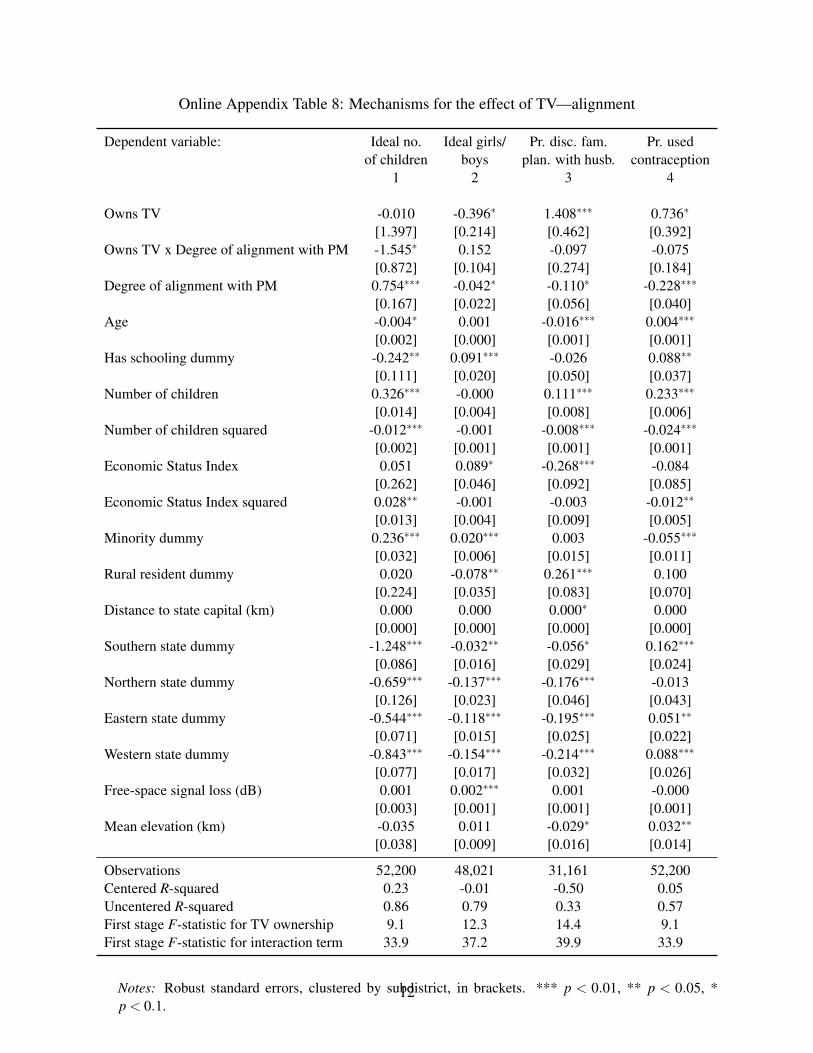
Online Appendix Table 8: Mechanisms for the effect of TV—alignment

Dependent variable: Ideal no. Ideal girls/ Pr. disc. fam. Pr. usedof children boys plan. with husb. contraception

1 2 3 4

Owns TV -0.010 -0.396∗ 1.408∗∗∗ 0.736∗

[1.397] [0.214] [0.462] [0.392]Owns TV x Degree of alignment with PM -1.545∗ 0.152 -0.097 -0.075

[0.872] [0.104] [0.274] [0.184]Degree of alignment with PM 0.754∗∗∗ -0.042∗ -0.110∗ -0.228∗∗∗

[0.167] [0.022] [0.056] [0.040]Age -0.004∗ 0.001 -0.016∗∗∗ 0.004∗∗∗

[0.002] [0.000] [0.001] [0.001]Has schooling dummy -0.242∗∗ 0.091∗∗∗ -0.026 0.088∗∗

[0.111] [0.020] [0.050] [0.037]Number of children 0.326∗∗∗ -0.000 0.111∗∗∗ 0.233∗∗∗

[0.014] [0.004] [0.008] [0.006]Number of children squared -0.012∗∗∗ -0.001 -0.008∗∗∗ -0.024∗∗∗

[0.002] [0.001] [0.001] [0.001]Economic Status Index 0.051 0.089∗ -0.268∗∗∗ -0.084

[0.262] [0.046] [0.092] [0.085]Economic Status Index squared 0.028∗∗ -0.001 -0.003 -0.012∗∗

[0.013] [0.004] [0.009] [0.005]Minority dummy 0.236∗∗∗ 0.020∗∗∗ 0.003 -0.055∗∗∗

[0.032] [0.006] [0.015] [0.011]Rural resident dummy 0.020 -0.078∗∗ 0.261∗∗∗ 0.100

[0.224] [0.035] [0.083] [0.070]Distance to state capital (km) 0.000 0.000 0.000∗ 0.000

[0.000] [0.000] [0.000] [0.000]Southern state dummy -1.248∗∗∗ -0.032∗∗ -0.056∗ 0.162∗∗∗

[0.086] [0.016] [0.029] [0.024]Northern state dummy -0.659∗∗∗ -0.137∗∗∗ -0.176∗∗∗ -0.013

[0.126] [0.023] [0.046] [0.043]Eastern state dummy -0.544∗∗∗ -0.118∗∗∗ -0.195∗∗∗ 0.051∗∗

[0.071] [0.015] [0.025] [0.022]Western state dummy -0.843∗∗∗ -0.154∗∗∗ -0.214∗∗∗ 0.088∗∗∗

[0.077] [0.017] [0.032] [0.026]Free-space signal loss (dB) 0.001 0.002∗∗∗ 0.001 -0.000

[0.003] [0.001] [0.001] [0.001]Mean elevation (km) -0.035 0.011 -0.029∗ 0.032∗∗

[0.038] [0.009] [0.016] [0.014]

Observations 52,200 48,021 31,161 52,200Centered R-squared 0.23 -0.01 -0.50 0.05Uncentered R-squared 0.86 0.79 0.33 0.57First stage F-statistic for TV ownership 9.1 12.3 14.4 9.1First stage F-statistic for interaction term 33.9 37.2 39.9 33.9

Notes: Robust standard errors, clustered by subdistrict, in brackets. *** p < 0.01, ** p < 0.05, *p < 0.1.

12

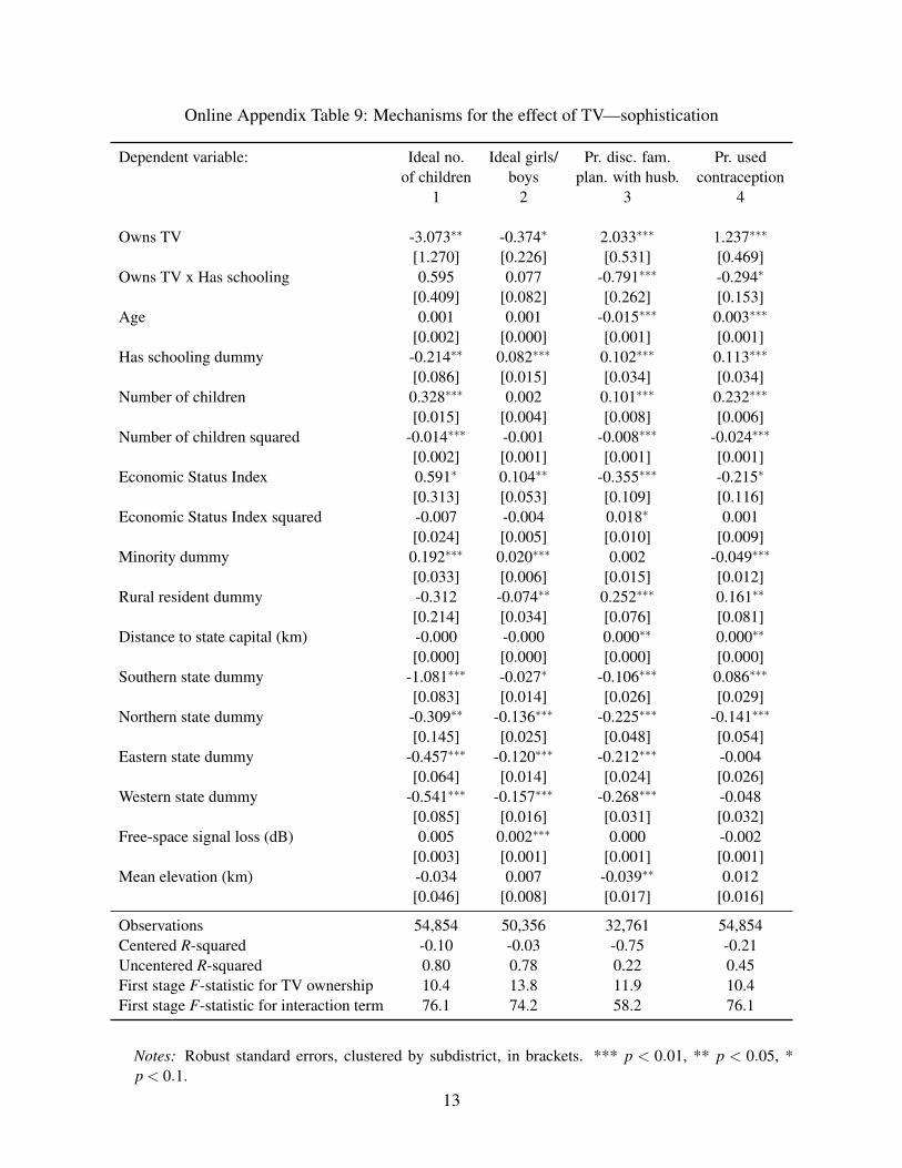
Online Appendix Table 9: Mechanisms for the effect of TV—sophistication

Dependent variable: Ideal no. Ideal girls/ Pr. disc. fam. Pr. usedof children boys plan. with husb. contraception

1 2 3 4

Owns TV -3.073∗∗ -0.374∗ 2.033∗∗∗ 1.237∗∗∗

[1.270] [0.226] [0.531] [0.469]Owns TV x Has schooling 0.595 0.077 -0.791∗∗∗ -0.294∗

[0.409] [0.082] [0.262] [0.153]Age 0.001 0.001 -0.015∗∗∗ 0.003∗∗∗

[0.002] [0.000] [0.001] [0.001]Has schooling dummy -0.214∗∗ 0.082∗∗∗ 0.102∗∗∗ 0.113∗∗∗

[0.086] [0.015] [0.034] [0.034]Number of children 0.328∗∗∗ 0.002 0.101∗∗∗ 0.232∗∗∗

[0.015] [0.004] [0.008] [0.006]Number of children squared -0.014∗∗∗ -0.001 -0.008∗∗∗ -0.024∗∗∗

[0.002] [0.001] [0.001] [0.001]Economic Status Index 0.591∗ 0.104∗∗ -0.355∗∗∗ -0.215∗

[0.313] [0.053] [0.109] [0.116]Economic Status Index squared -0.007 -0.004 0.018∗ 0.001

[0.024] [0.005] [0.010] [0.009]Minority dummy 0.192∗∗∗ 0.020∗∗∗ 0.002 -0.049∗∗∗

[0.033] [0.006] [0.015] [0.012]Rural resident dummy -0.312 -0.074∗∗ 0.252∗∗∗ 0.161∗∗

[0.214] [0.034] [0.076] [0.081]Distance to state capital (km) -0.000 -0.000 0.000∗∗ 0.000∗∗

[0.000] [0.000] [0.000] [0.000]Southern state dummy -1.081∗∗∗ -0.027∗ -0.106∗∗∗ 0.086∗∗∗

[0.083] [0.014] [0.026] [0.029]Northern state dummy -0.309∗∗ -0.136∗∗∗ -0.225∗∗∗ -0.141∗∗∗

[0.145] [0.025] [0.048] [0.054]Eastern state dummy -0.457∗∗∗ -0.120∗∗∗ -0.212∗∗∗ -0.004

[0.064] [0.014] [0.024] [0.026]Western state dummy -0.541∗∗∗ -0.157∗∗∗ -0.268∗∗∗ -0.048

[0.085] [0.016] [0.031] [0.032]Free-space signal loss (dB) 0.005 0.002∗∗∗ 0.000 -0.002

[0.003] [0.001] [0.001] [0.001]Mean elevation (km) -0.034 0.007 -0.039∗∗ 0.012

[0.046] [0.008] [0.017] [0.016]

Observations 54,854 50,356 32,761 54,854Centered R-squared -0.10 -0.03 -0.75 -0.21Uncentered R-squared 0.80 0.78 0.22 0.45First stage F-statistic for TV ownership 10.4 13.8 11.9 10.4First stage F-statistic for interaction term 76.1 74.2 58.2 76.1

Notes: Robust standard errors, clustered by subdistrict, in brackets. *** p < 0.01, ** p < 0.05, *p < 0.1.

13

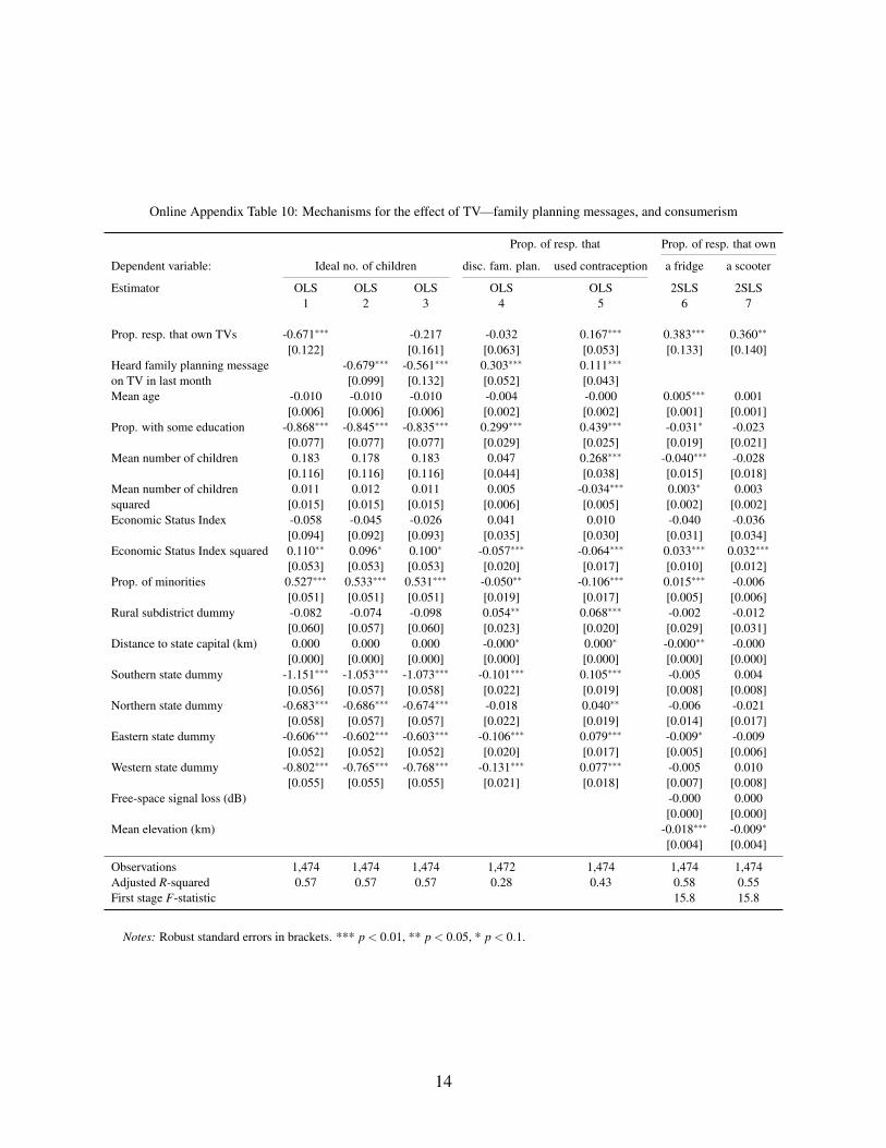
Online Appendix Table 10: Mechanisms for the effect of TV—family planning messages, and consumerism

Prop. of resp. that Prop. of resp. that own

Dependent variable: Ideal no. of children disc. fam. plan. used contraception a fridge a scooter

Estimator OLS OLS OLS OLS OLS 2SLS 2SLS1 2 3 4 5 6 7

Prop. resp. that own TVs -0.671∗∗∗ -0.217 -0.032 0.167∗∗∗ 0.383∗∗∗ 0.360∗∗

[0.122] [0.161] [0.063] [0.053] [0.133] [0.140]Heard family planning message -0.679∗∗∗ -0.561∗∗∗ 0.303∗∗∗ 0.111∗∗∗

on TV in last month [0.099] [0.132] [0.052] [0.043]Mean age -0.010 -0.010 -0.010 -0.004 -0.000 0.005∗∗∗ 0.001

[0.006] [0.006] [0.006] [0.002] [0.002] [0.001] [0.001]Prop. with some education -0.868∗∗∗ -0.845∗∗∗ -0.835∗∗∗ 0.299∗∗∗ 0.439∗∗∗ -0.031∗ -0.023

[0.077] [0.077] [0.077] [0.029] [0.025] [0.019] [0.021]Mean number of children 0.183 0.178 0.183 0.047 0.268∗∗∗ -0.040∗∗∗ -0.028

[0.116] [0.116] [0.116] [0.044] [0.038] [0.015] [0.018]Mean number of children 0.011 0.012 0.011 0.005 -0.034∗∗∗ 0.003∗ 0.003squared [0.015] [0.015] [0.015] [0.006] [0.005] [0.002] [0.002]Economic Status Index -0.058 -0.045 -0.026 0.041 0.010 -0.040 -0.036

[0.094] [0.092] [0.093] [0.035] [0.030] [0.031] [0.034]Economic Status Index squared 0.110∗∗ 0.096∗ 0.100∗ -0.057∗∗∗ -0.064∗∗∗ 0.033∗∗∗ 0.032∗∗∗

[0.053] [0.053] [0.053] [0.020] [0.017] [0.010] [0.012]Prop. of minorities 0.527∗∗∗ 0.533∗∗∗ 0.531∗∗∗ -0.050∗∗ -0.106∗∗∗ 0.015∗∗∗ -0.006

[0.051] [0.051] [0.051] [0.019] [0.017] [0.005] [0.006]Rural subdistrict dummy -0.082 -0.074 -0.098 0.054∗∗ 0.068∗∗∗ -0.002 -0.012

[0.060] [0.057] [0.060] [0.023] [0.020] [0.029] [0.031]Distance to state capital (km) 0.000 0.000 0.000 -0.000∗ 0.000∗ -0.000∗∗ -0.000

[0.000] [0.000] [0.000] [0.000] [0.000] [0.000] [0.000]Southern state dummy -1.151∗∗∗ -1.053∗∗∗ -1.073∗∗∗ -0.101∗∗∗ 0.105∗∗∗ -0.005 0.004

[0.056] [0.057] [0.058] [0.022] [0.019] [0.008] [0.008]Northern state dummy -0.683∗∗∗ -0.686∗∗∗ -0.674∗∗∗ -0.018 0.040∗∗ -0.006 -0.021

[0.058] [0.057] [0.057] [0.022] [0.019] [0.014] [0.017]Eastern state dummy -0.606∗∗∗ -0.602∗∗∗ -0.603∗∗∗ -0.106∗∗∗ 0.079∗∗∗ -0.009∗ -0.009

[0.052] [0.052] [0.052] [0.020] [0.017] [0.005] [0.006]Western state dummy -0.802∗∗∗ -0.765∗∗∗ -0.768∗∗∗ -0.131∗∗∗ 0.077∗∗∗ -0.005 0.010

[0.055] [0.055] [0.055] [0.021] [0.018] [0.007] [0.008]Free-space signal loss (dB) -0.000 0.000

[0.000] [0.000]Mean elevation (km) -0.018∗∗∗ -0.009∗

[0.004] [0.004]

Observations 1,474 1,474 1,474 1,472 1,474 1,474 1,474Adjusted R-squared 0.57 0.57 0.57 0.28 0.43 0.58 0.55First stage F-statistic 15.8 15.8

Notes: Robust standard errors in brackets. *** p < 0.01, ** p < 0.05, * p < 0.1.

14

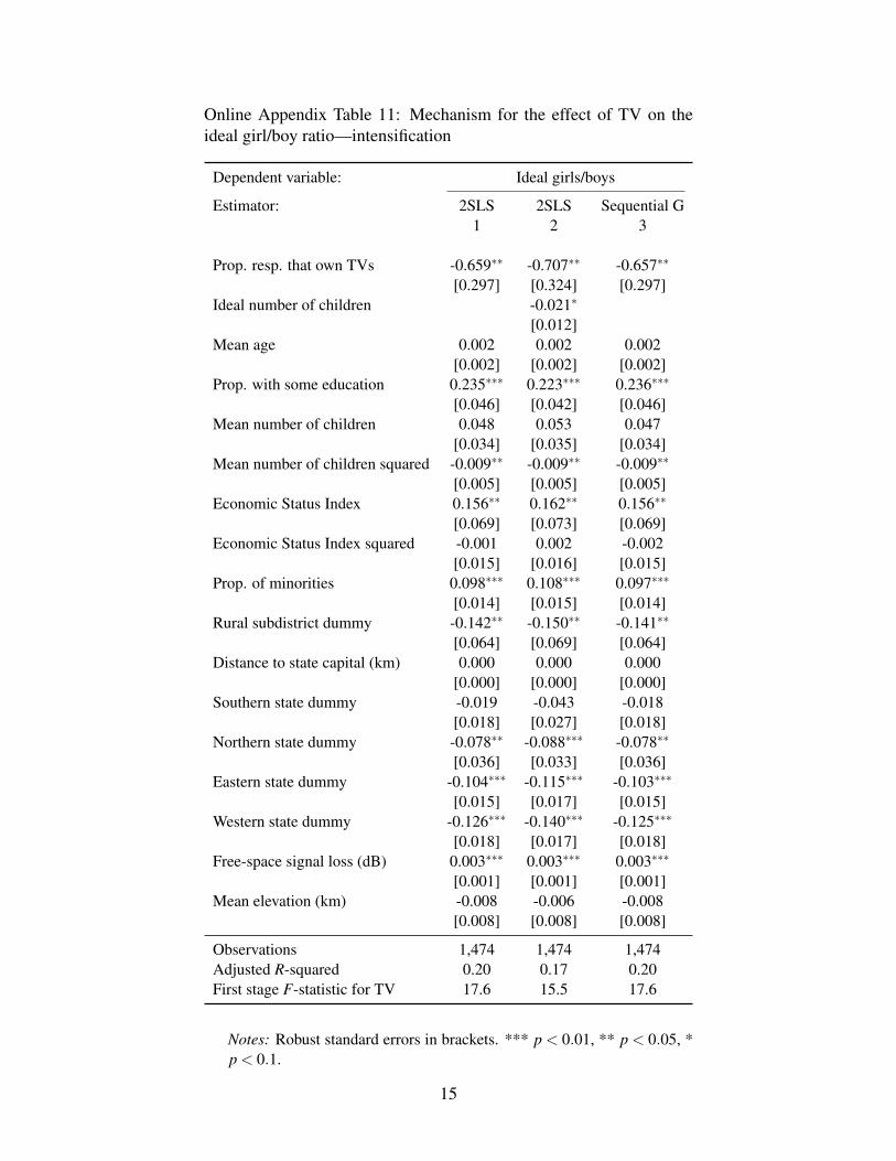
Online Appendix Table 11: Mechanism for the effect of TV on theideal girl/boy ratio—intensification

Dependent variable: Ideal girls/boys

Estimator: 2SLS 2SLS Sequential G1 2 3

Prop. resp. that own TVs -0.659∗∗ -0.707∗∗ -0.657∗∗

[0.297] [0.324] [0.297]Ideal number of children -0.021∗

[0.012]Mean age 0.002 0.002 0.002

[0.002] [0.002] [0.002]Prop. with some education 0.235∗∗∗ 0.223∗∗∗ 0.236∗∗∗

[0.046] [0.042] [0.046]Mean number of children 0.048 0.053 0.047

[0.034] [0.035] [0.034]Mean number of children squared -0.009∗∗ -0.009∗∗ -0.009∗∗

[0.005] [0.005] [0.005]Economic Status Index 0.156∗∗ 0.162∗∗ 0.156∗∗

[0.069] [0.073] [0.069]Economic Status Index squared -0.001 0.002 -0.002

[0.015] [0.016] [0.015]Prop. of minorities 0.098∗∗∗ 0.108∗∗∗ 0.097∗∗∗

[0.014] [0.015] [0.014]Rural subdistrict dummy -0.142∗∗ -0.150∗∗ -0.141∗∗

[0.064] [0.069] [0.064]Distance to state capital (km) 0.000 0.000 0.000

[0.000] [0.000] [0.000]Southern state dummy -0.019 -0.043 -0.018

[0.018] [0.027] [0.018]Northern state dummy -0.078∗∗ -0.088∗∗∗ -0.078∗∗

[0.036] [0.033] [0.036]Eastern state dummy -0.104∗∗∗ -0.115∗∗∗ -0.103∗∗∗

[0.015] [0.017] [0.015]Western state dummy -0.126∗∗∗ -0.140∗∗∗ -0.125∗∗∗

[0.018] [0.017] [0.018]Free-space signal loss (dB) 0.003∗∗∗ 0.003∗∗∗ 0.003∗∗∗

[0.001] [0.001] [0.001]Mean elevation (km) -0.008 -0.006 -0.008

[0.008] [0.008] [0.008]

Observations 1,474 1,474 1,474Adjusted R-squared 0.20 0.17 0.20First stage F-statistic for TV 17.6 15.5 17.6

Notes: Robust standard errors in brackets. *** p < 0.01, ** p < 0.05, *p < 0.1.

15

Dataset construction

The original NFHS–1 dataset includes 76,552 women respondents. We drop the following ob-

servations: those not in the sampling frame (5), visitors since we assume they were not exposed

to the media in the subdistrict (5,579), those with the dependent variable missing (6,774), those

missing education (1), and women who want more than 7 children (551). 8,366 observations were

dropped in the course of constructing the instrument, since the NFHS fails to identify the district

these respondents are in (we need this in order to assign effective signal loss to each data point).

We took the following steps to construct the instrumental variable (Effective signal loss) and

the key control variable (Free space loss):

1. Use GIS to provide the centroid coordinate of every subdistrict in India, based on the sub-

district maps in the 2001 Census of India (the next census after the NFHS–1).

2. Calculate Effective signal loss and Free space loss for every transmitter-subsdistrict centroid

pair, and, from among all these permutations, keep only the calculation yielding the strongest

signal.

3. Classify every subdistrict as either rural or urban: rural subdistricts are those in which

greater than 50% of the population is described as rural in the 2001 Census; urban sub-

districts are those in which less than 50% of the population is described as rural in the 2001

Census.

4. Calculate the average rural ITM for the district by taking the average Effective signal loss

and the average Free space loss of all rural subdistricts in the district; calculate the average

urban ITM for the district by taking the average Effective signal loss and the average Free

space loss of all urban subdistricts in the district. These serve as the key instruments.

16

References

Ellington, HI, E Addinall and MC Hately. 1980. “The physics of television broadcasting.” Physics

Education 15(4):222.

17