Calibrating the SABR Model to

Noisy FX Data

Kellogg College

University of Oxford

A thesis submitted in partial fulfillment of the MSc in

Mathematical Finance

Hilary 2018

Abstract

We consider the problem of fitting the SABR model to an FX volatility

smile. It is demonstrated that the model parameter β cannot be deter-

mined from a log-log plot of σATM against F . It is also shown that, in an

FX setting, the SABR model has a single state variable. A new method

is proposed for fitting the SABR model to observed quotes. In contrast to

the fitting techniques proposed in the literature, the new method allows

all the SABR parameters to be retrieved and does not require prior beliefs

about the market. The effect of noise on the new fitting technique is also

investigated.

Acknowledgements

I would like to thank both of my supervisors Dr Daniel Jones and Guil-

laume Bigonzi for their guidance and support throughout this project.

They provided the direction for this work and offered invaluable insight

and advice along the way. I also gratefully acknowledge the financial

support from Bank Julius Baer and Co. Ltd. Finally I thank Dr Beate

Solleder for her love and tireless support and for tolerating me during the

time it has taken me to complete this project.

1 Introduction

The work presented here is concerned with fitting the SABR stochastic volatility

model to foreign exchange (FX) data. Specifically, we are interested in the implied

volatility of an option, σ, as a function of the strike of the option, K. This relation-

ship between σ and K is known as the volatility smile. For specified SABR model

parameters, the volatility smile is given by the well known equation of Hagan et al. [1].

Here we focus on the inverse problem, i.e. given a volatility smile which was generated

using the SABR model, how can we obtain the parameters of the underlying SABR

model?

In section 2 we introduce the quoting conventions used in the FX market and

define the three options which are commonly used to describe the FX volatility smile.

A method for calibrating a volatility smile to market quotes is also described. The

SABR model is presented in section 3 and the equations which will be used throughout

this work are stated. Section 4 reviews previous works related to fitting the SABR

model to market data and section 5 gives details of the Monte Carlo method which

was used to generate simulated market data. In this work we have focused on fitting

simulated data since this removes any uncertainty regarding whether the SABR model

accurately describes the market and what the true model parameters are.

A key topic when fitting the SABR model to market data is the determination

of the parameter β. In section 6 we explain why an approach to fitting β that is

often described in the literature does not produce reliable results. Section 7 examines

whether variance-covariance matching can be used to estimate the SABR parameters

from time series of σATM and F . The relationship between the three main FX options

quotes that would be predicted by the SABR model is investigated in section 8.

These predictions are also compared to sample market data. An approximation for

the correlation between the implied volatility at-the-money and the forward price is

considered in section 9. This correlation is important because it allows vega exposure

to be partially hedged with delta.

A new method for fitting the SABR model to FX data is proposed in section 10

and the ability of this method to retrieve the parameters of the underlying SABR

model is investigated. We begin with the case that the quotes are free from noise

and then systematically introduce noise on each of the three main option quotes.

Section 11 considers the case of pricing a digital option when the volatility smile is

described using the SABR model. Conclusions are drawn in section 12, which also

includes suggestions for further work.

1

2 Introduction to FX Market Conventions

The foreign exchange (FX) market is one of the most liquid and competitive mar-

kets in the world. Because many of the FX market conventions are unique to this

market, this section provides a brief introduction to these conventions. In the FX

market participants agree to exchange one currency for another on a specified day

at a specified FX rate. An FX rate is the price of one currency expressed in terms

of another currency. Consider the currency pair XXXYYY. The tag XXX represents

the “foreign” currency, while YYY represents the “domestic” currency. The FX rate

XXXYYY specifies the price of the foreign currency in terms of the domestic currency.

For example; EURUSD specifies the price of one Euro in US dollars.

This section begins with an explanation of the delta conventions which are used

for quoting options in the FX market. Thereafter we introduce three commonly

traded options structures: the at-the-money straddle, risk reversal and vega-weighted

butterfly. These three structures are particularly important because they are often

used to define the volatility smile in the FX market. The section concludes with a

description of a method for calibrating a volatility smile to observed market prices.

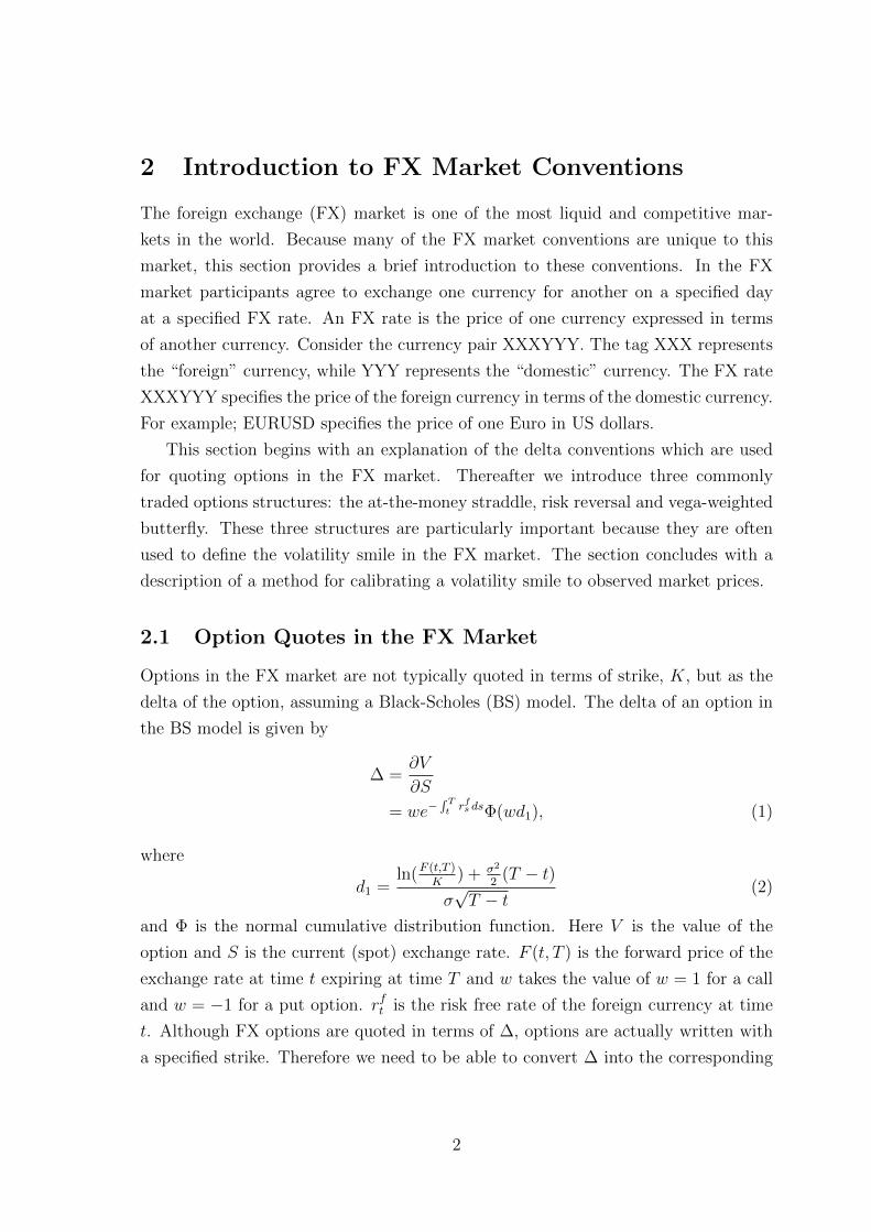
2.1 Option Quotes in the FX Market

Options in the FX market are not typically quoted in terms of strike, K, but as the

delta of the option, assuming a Black-Scholes (BS) model. The delta of an option in

the BS model is given by

∆ =∂V

∂S

= we−∫ Tt rfs dsΦ(wd1), (1)

where

d1 =ln(F (t,T )

K) + σ2

2(T − t)

σ√T − t

(2)

and Φ is the normal cumulative distribution function. Here V is the value of the

option and S is the current (spot) exchange rate. F (t, T ) is the forward price of the

exchange rate at time t expiring at time T and w takes the value of w = 1 for a call

and w = −1 for a put option. rft is the risk free rate of the foreign currency at time

t. Although FX options are quoted in terms of ∆, options are actually written with

a specified strike. Therefore we need to be able to convert ∆ into the corresponding

2

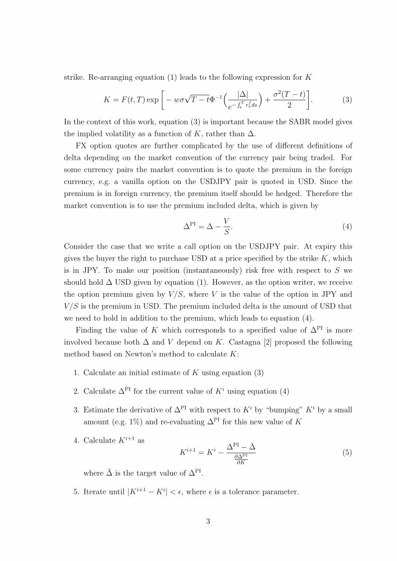
strike. Re-arranging equation (1) leads to the following expression for K

K = F (t, T ) exp

[− wσ

√T − tΦ−1

( |∆|e−

∫ Tt rfs ds

)+σ2(T − t)

2

]. (3)

In the context of this work, equation (3) is important because the SABR model gives

the implied volatility as a function of K, rather than ∆.

FX option quotes are further complicated by the use of different definitions of

delta depending on the market convention of the currency pair being traded. For

some currency pairs the market convention is to quote the premium in the foreign

currency, e.g. a vanilla option on the USDJPY pair is quoted in USD. Since the

premium is in foreign currency, the premium itself should be hedged. Therefore the

market convention is to use the premium included delta, which is given by

∆PI = ∆− V

S. (4)

Consider the case that we write a call option on the USDJPY pair. At expiry this

gives the buyer the right to purchase USD at a price specified by the strike K, which

is in JPY. To make our position (instantaneously) risk free with respect to S we

should hold ∆ USD given by equation (1). However, as the option writer, we receive

the option premium given by V/S, where V is the value of the option in JPY and

V/S is the premium in USD. The premium included delta is the amount of USD that

we need to hold in addition to the premium, which leads to equation (4).

Finding the value of K which corresponds to a specified value of ∆PI is more

involved because both ∆ and V depend on K. Castagna [2] proposed the following

method based on Newton’s method to calculate K:

1. Calculate an initial estimate of K using equation (3)

2. Calculate ∆PI for the current value of Ki using equation (4)

3. Estimate the derivative of ∆PI with respect to Ki by “bumping” Ki by a small

amount (e.g. 1%) and re-evaluating ∆PI for this new value of K

4. Calculate Ki+1 as

Ki+1 = Ki − ∆PI − ∆∂∆PI

∂K

(5)

where ∆ is the target value of ∆PI.

5. Iterate until |Ki+1 −Ki| < ε, where ε is a tolerance parameter.

3

2.2 At-the-money Straddle

The most liquid FX option is the at-the-money (ATM) straddle. This structure

consists of a call and put both struck at the “at-the-money” level. The definition of

the ATM strike depends on market conventions. One choice is the zero delta ATM

strike, which is defined as the strike that leads to the call and the put having the same

delta (but with opposite sign). Another possible definition of the ATM strike is the

ATM forward. Under this convention the ATM strike is set equal to the forward price

of the underlying currency pair with the same expiry as the option. By no-arbitrage

the forward price is given by

F (t, T ) = Ste−

∫ Tt rfs ds

e−∫ Tt rdsds

, (6)

where rdt is the risk free rate of the domestic currency at time t. The final definition

of the ATM strike is the at-the-money spot, where the ATM strike is defined to be

S, the current spot rate of the underlying pair.

The at-the-money straddle describes the level of the implied volatility surface:

changing the ATM volatility results in a parallel shift of the implied volatility surface

along the implied volatility axis.

2.3 Risk Reversal

A risk reversal is a highly-traded structure consisting of a long call and a short put.

The call and put are symmetric in that they are chosen to have the same delta (but

with opposite sign). The most commonly traded risk reversal contract is the 25 delta

contract, where the call and put are stuck such that they have deltas of 0.25 and -0.25,

respectively. In the market, the risk reversal is quoted as the difference between the

implied volatilities of the call and the put, i.e.

σ25RR(t, T ) = σ25C(t, T )− σ25P (t, T ). (7)

The risk reversal can be either positive or negative and describes the skew of the

implied volatility surface. A positive risk reversal indicates that there is more demand

for calls than puts, whereas a negative risk reversal suggests that puts are favoured

over calls.

4

2.4 Butterfly

A vega-weighted butterfly (VWB) is a highly-traded structure consisting of a long

call, a long put and a short ATM straddle. The long call and long put are again

symmetric in delta and together form a strangle. For the most commonly traded

butterfly, delta is again chosen to be 0.25 for the call and -0.25 for the put. This is

referred to as the 25 delta butterfly. The vega of the strangle is larger than that of

the ATM straddle meaning that the quantity of the straddle needs to be larger than

the quantity of the strangle in order that the structure is vega neutral. The market

quote for the VWB is defined as the difference between the volatility of the strangle

and the volatility of the ATM straddle (σATM).

Market quotes for the vega-weighted butterfly are complicated by the existence of

two conventions for the strangle. The most straight forward definition of the strangle

is to use the same put and call options which were used for the risk reversal. This

results in the ‘two-vol’ butterfly, which is defined as

σ25BF(t, T ) =1

2

[σ25C(t, T ) + σ25P (t, T )

]− σATM(t, T ). (8)

Under this convention the volatility of the strangle is defined as the mean of the

volatilities of the put and the call.

However, the most common market quote for the VWB is not the two-vol butterfly,

but the single-vol butterfly. In this case the volatilities of the put and the call are

chosen to be equal to one another. Define σVWB to be the volatility of the put and

the call for the single-vol strangle. The market quote for the single-vol butterfly is

then

σ1−vol−25BF(t, T ) = σVWB(t, T )− σATM(t, T ). (9)

For σ25RR = 0, equation (8) reduces to equation (9) and the two conventions for

VWB are equivalent. In general, however, the two definitions are not equivalent and

the discrepancy between σ25BF and σ1−vol−25BF tends to increase as the magnitude

of σ25RR increases. Either σ25BF or σ1−vol−25BF can be used to construct a volatility

smile. What is important is to understand which convention is being used and how to

interpret the market quotes in term of the constraints that they place on the volatility

smile. For simplicity the majority of this work has been performed using the two-vol

butterfly, σ25BF. This choice means that fewer strikes are required in the calibration

process. Section 2.5 describes how to calibrate a volatility smile using market quotes

for σ1−vol−25BF, which is the case that will be most frequently encountered in practice.

5

The butterfly describes the curvature of the implied volatility surface; a high value

of σ25BF(t, T ) implies that the implied volatility in the wings is large compared to the

implied volatility at-the-money.

2.5 Building the Volatility Smile from Market Data

The volatility smile is a mapping between strike, K, and implied volatility:

K 7→ σ(K). (10)

In this section it is assumed that we have a functional form for σ(K) which we wish

to fit to market quotes for σATM, σ25RR and σ1−vol−25BF. This is the case that is most

frequently encountered in practice. It is assumed further that, given three points on

the volatility smile, we can fit the function σ(K) such that we can obtain the volatility

for any K ≥ 0. Although this work focuses on fitting the SABR model, the method

described below can be applied to any functional form which meets these criteria.

For example, the vanna-vega interpolation method proposed by Castagna [2] or the

simplified parabolic interpolation method introduced by Reiswich [3].

Constructing the volatility smile from market data is achieved by recognising

the three constraints placed on the smile by the three options quotes discussed

above (σATM, σ25RR and σ1−vol−25BF). These constraints are described in detail by

Reiswich [3] and Castagna [2]. The market quote for σATM provides the constraint

σ(KATM) = σATM, (11)

where KATM is determined by market conventions. To ensure that σ25RR is priced

correctly by the volatility smile we have

σ(K25C)− σ(K25P) = σ25RR. (12)

Here the strikes K25C and K25P fulfil

∆∗(K25C, σ(K25C)) = 0.25,

∆∗(K25P, σ(K25P)) = −0.25. (13)

The function ∆∗(K, σ) is either the standard delta or the premium included delta and

is determined by market conventions. The final constraint is that the value of a VWB

priced by the volatility smile should match the price quoted in the market. Here we

6

assume that the market quote for the VWB uses the single volatility convention. The

put and call that make up the VWB have a volatility given by

σVWB(t, T ) = σ1−vol−25BF(t, T ) + σATM(t, T ). (14)

The strikes of these options can be found by solving the equations

∆∗(K25C, σVWB) = 0.25,

∆∗(K25P, σVWB) = −0.25 (15)

for K25C and K25P. The value of the strangle component of the VWB is:

C(K25C, σVWB) + P (K25P, σVWB). (16)

Here C(K, σ) and P (K, σ) are, respectively, the Black-Scholes price of a call (put)

option with strike K and volatility σ. The volatility smile must be able to reproduce

the price of this strangle, which leads to

C(K25C, σVWB) + P (K25P, σVWB) = C(K25C, σ(K25C)

)+ P

(K25P, σ(K25P)

). (17)

Castagna [2] proposed the following method to generate a volatility smile based

on market prices of the ATM straddle, risk reversal and single-vol butterfly. First the

ATM strike is determined from σATM. If the market convention is a zero delta ATM

strike and the premium is not included in delta, KATM is given by

KATM = F (t, T )e12σ2ATM(T−t). (18)

For a put and a call to have the same strike and absolute value of delta we require

Φ(d1) = Φ(−d1), which implies d1 = 0. Equation (18) arises from re-arraning equa-

tion (2) with d1 = 0. When the premium is included, the ATM strike is calculated

as

KATM = F (t, T )e−12σ2ATM(T−t). (19)

Equation (19) arises from equating the sum of ∆PI for a put and a call to zero. This

leads to Φ(d2) = Φ(−d2) where

d2 =ln(F (t,T )

K)− σ2

2(T − t)

σ√T − t

(20)

Re-arraning equation (20) with d2 = 0 yields equation (19).

7

If market convention dictates that the strike is either the forward price or the spot

price, then KATM can be observed directly in the market. The 25 delta strikes for the

25 delta VWB are calculated as

K25P = F (t, T )eσVWB

√(T−t)Φ−1(0.25e

∫Tt r

fs ds)+ 1

2σ2VWB(T−t) (21)

K25C = F (t, T )e−σVWB

√(T−t)Φ−1(0.25e

∫Tt r

fs ds)+ 1

2σ2VWB(T−t) (22)

When the premium is included in the delta K25P and K25C must be calculated using

the procedure described in section 2.1.

Next an iterative procedure is used to determine the two 25 delta volatilities in

terms of an equivalent VWB volatility σie. This procedure ensures that the price of

a VWB is equal to the sum of the prices of the call and put options from which it is

composed. The iterative procedure requires values for the first two iterations of σie to

be specified. This is because the derivative of the fitting error with respect to σie is

estimated using finite differences. Initial values of σ0e = σ1−vol−25BF and σ1

e = σ0e+10−4

are typically chosen. FX volatilities are normally around 10%, meaning that a “bump”

size of 10−4 will normally yield a satisfactory approximation of the derivative of the

fitting error with respect to σie. The iterative procedure consists of the following steps:

1. Calculate the implied 25 delta volatilities as

σ25P = σATM + σie − σ25RR

σ25C = σATM + σie + σ25RR

2. Determine the strikes corresponding to these volatilities

Ki25P = F (t, T )eσ25P

√(T−t)Φ−1(0.25e

∫Tt r

fs ds)+ 1

2σ225P (T−t)

Ki25C = F (t, T )e−σ25C

√(T−t)Φ−1(0.25e

∫Tt r

fs ds)+ 1

2σ225C(T−t)

When the premium is included in delta, the procedure described in section 2.1

must be use to determine Ki25P and Ki

25C .

3. Calibrate the function σ(K) to the volatilities at Ki25P , Ki

25C and KATM. Use

the calibrated curve to find the implied volatilities at K25P and K25C .

4. Calculate the price difference between a butterfly strangle calculated using σVWB

and the same strangle priced using the volatilities found above:

Ei =C(K25C , σ(K25C)) + P (K25P , σ(K25P ))

−C(K25C , σVWB)− P (K25P , σVWB).

8

5. If this is not the first iteration then update σie using Newton’s method:

σi+1e = σie −

Ei

∂Ei

∂σie

where

∂Ei

∂σie≈ Ei − Ei−1

σie − σi−1e

6. Iterate until Ei < ε for a suitably small value of ε. Note that, since the ini-

tial bump size (in this case chosen to be 10−4) serves only to allow ∂Ei

∂σieto be

estimated, ε can be chosen independently from the choice for the initial bump.

9

3 The SABR model

This work is concerned with calibrating the SABR model to FX data. This section

introduces the SABR model and quotes the formulae which will be used throughout

this work.

The SABR model was proposed by Hagan et al. [1]. It is a stochastic volatility

model which describes the evolution of the forward price of an asset, F (t), as

dF = αF βdW 1, F (t = 0) = F0, (23)

dα = vαdW 2, α(t = 0) = α0,

where W 1 and W 2 are two correlated Brownian motions with

d〈W 1,W 2〉 = ρdt. (24)

Hagan et al. [1] showed that for this model the implied volatility of an option with

strike K can be approximated by

σ(K,F ) =α0

(FK)(1−β)/2(1 + (1−β)2

24log2 F/K + (1−β)4

1920log4 F/K + ...

) .( z

x(z)

).(

1 +[(1− β)2

24

α20

(FK)1−β +1

4

ρβα0v

(FK)1−β2

+2− 3ρ2

24v2][T − t

]+ ...

)(25)

where

z =v

α0

(FK)(1−β)/2 logF/K (26)

and

x(z) = log

(√1− 2ρz + z2 + z − ρ

1− ρ

). (27)

Note that the stochastic processes α and F are treated somewhat inconsistently in

equation (25). While it is stressed that σ depends on the value of α at t = 0, F enters

equation (25) as a process. In practice, we would apply equation (25) to calculate σ

when t = 0 and α and F are known, i.e. to be consistent with the treatment of α, the

F entering equation (25) should be F0. However, when analysing the SABR model

it is often useful to consider what happens as F0 and α0 vary. To this end we abuse

notation and drop the subscripts in equation (25). That is the α and F entering

equation (25) are stochastic processes governed by equation (23) and whenever we

wish to evaluate σ we set t = 0 and observe the current realisations of α and F .

10

For the special case of options struck at the forward price, equation (25) reduces

to

σATM = σ(F, F )

=α

F 1−β

(1 +

[(1− β)2

24

α2

F 2−2β+

1

4

ρβαv

F 1−β +2− 3ρ2

24v2][T − t

]+ ...

)(28)

Note that we have assumed that the ATM strike is given by the forward price, F . For

simplicity, this convention will be adopted throughout the remainder of this work.

Hagan et al. [1] noted that the (T − t) term is usually less than 1 or 2 %. Ta-

ble 1 shows the order of magnitude of the SABR parameters for a typical FX volatility

smile. For these values, the (T−t) term is dominated by the final term and is approx-

imately 224v2(T − t). This term is dimensionless (as expected) and is approximately

2%, which is in agreement with Hagan et al. [1].

Table 1: Typical SABR parameters for FX options.

F α ρ β v T − t1.0 0.1 0.1 1.0 1.0 0.25

3.1 The “Backbone” of the Volatility Smile

In the context of the SABR model, the term “backbone” is used to describe the curve

traced out by σATM as the forward price varies. Hagan et al. [1] argued that the

(T − t) term in equation (28) can usually be ignored when analysing the behaviour

of the backbone. Taking logarithms of equation (28) and ignoring the (T − t) term

gives

log(σATM) = log(α)− (1− β) log(F ). (29)

Equation (29) indicates that σATM ∝ F−(1−β). To gain insight into this relationship,

consider the two limiting cases of β = 1 and β = 0. When β = 1, F can be written

as

FT = F0 exp

(∫ T

0

αdw − 1

2

∫ T

0

α2ds

). (30)

11

Assuming zero interest rate, the value of a call option on F with strike K = F0 is

C(F0) = E[

max(FT − F0, 0))]

= F0E[

max(

exp( ∫ T

0

αdw − 1

2

∫ T

0

α2ds)− 1), 0

].

The expectation is independent of F0, meaning that the option price is proportional

to the forward price.

For β = 0, F can be written as

FT = F0 +

∫ T

0

αdw. (31)

In this case the value of a call option on F with strike K = F0 is

C(F0) = E[

max(∫ T

0

αdw, 0)]. (32)

The expectation is again independent of F0, meaning that the option price is inde-

pendent of F0.

For a call struck at-the-money, the Black-Scholes price is

C(F, t) = FN(d1)− F0N(d2), (33)

where

d1 = −d2 =1

2σimp√T − t. (34)

At inception, t = 0 and F = F0. Rearranging gives

N(d1) =C(F0, 0)

2F0

+1

2. (35)

Therefore the implied volatility is given by

σimp =2√T − t

N−1(C(F0, 0)

2F0

+1

2

). (36)

For small C(F0,0)F0

, σimp is approximately linear in C(F0,0)F0

. We can use this relation to

convert the trends we have noted for C(F0) into trends for σimp. Thus, for β = 1,

we expect that σimp is independent of F0, whereas for β = 0, we predict that σimp is

proportional to F−10 .

Hagan et al. [1] state that the “backbone”, which they define as the curve that

σATM traces as F varies, is determined almost entirely by β: β = 1 gives a flat

12

backbone, whereas β = 0 produces a downward sloping backbone. This behaviour,

which is described by equation (29), is exactly what we obtained above by considering

the behaviour of σimp as a function of F0. We prefer to define the backbone as the

curve that σimp traces as F0 varies because this emphasises that all other parameters,

and in particular α, are held constant. In practice, the backbone will be difficult to

observe in market data because the Brownian motions driving F and α are correlated.

This is discussed in more detail in section 6.

3.2 Refinement of the SABR model

Obloj [4] compared the formulae presented by Hagan et al. [1] and Berestycki et

al. [5] and found a discrepancy for β < 1. Based on this analysis, Obloj [4] proposed

a corrected version of the formula derived by Hagan et al. Obloj [4] wrote the implied

volatility as a Taylor expansion in the time to maturity (T − t) as

σ(K,F ) = σ0(K,F )

(1 + σ1(K,F )(T − t)

)+O((T − t)2), (37)

where

σ1(K,F ) =(1− β)2

24

α2

(FK)1−β +1

4

ρβαv

(FK)1−β2

+2− 3ρ2

24v2,

σ0(K,F ) =v ln F

K

ln(√

1−2ρζ+ζ2+ζ−ρ1−ρ

) ,ζ =

v

α

F 1−β −K1−β

1− β.

Comparing equation (28) and (37) we see that the discrepancy between Hagan et al.

and Obloj occurs in the value of σ0(K,F ). The main result of Obloj [4] is to correct

the zx(z)

term in equation (28). Simple calculations show that both formulations of

the zx(z)

term yield the same result when F = K, or when v = 0, or when β = 1;

see Obloj [4] for details. In addition, Obloj truncated the expansion in log FK

in the

denominator of σ0(K,F ) to leading-order. In this work equation (37) will be used to

describe the implied volatility of the SABR model.

13

4 Literature Survey: Calibrating the SABR Model

We now review the literature relating to the main topic of this work: calibration

methods for the SABR model. Different methods have been proposed for estimating

the SABR parameters from market data. The choice of β and whether it is fitted to

market data or selected in advance, is a particularly important topic in the field of

calibrating the SABR model.

Hagan et al. [1] introduced the SABR model and derived equations for the implied

volatility as a function of strike for the model. It was noted that the parameters β

and ρ affect the volatility smile in similar ways since both influence the skew. Indeed

the authors showed an example volatility smile which could be equally well fitted by

the SABR model with β = 0 or β = 1. Hagan et al. [1] noted that this redundancy

makes it difficult to fit both β and ρ from a single market snapshot. The authors

proposed using a log-log plot of historic values of σATM against F to determine β.

Based on equation (29) it was argued that β can be found from the gradient of such

a plot. Alternatively, Hagan et al. [1] recommended selecting a value of β based on

prior beliefs about the market.

West [6] calibrated the SABR model to illiquid South African markets. They used

a log-log plot of σATM against F to determine β and found that β was a function of

time. The model was also calibrated using a single value of β = 0.7 and it was found

that this choice led to more stable values for the other SABR parameters. Based on

these data, West [6] recommended fixing β for the life of a contract. We will see in

section 6 that β cannot be determined from a log-log plot of historical values of σATM

against F because the slope of this plot is also influenced by ρ. Evidence of this can

be seen in the data presented by West [6], which show a strong correlation between

the time series of β and ρ.

Nowak and Sibetz [7] fitted the Heston and SABR models to FX data. They

proposed fitting β using a log-log plot of σATM against F or using a value of β

based on prior beliefs. Two approaches were considered for fitting the remaining

three parameters. In the first approach α, ρ and v were found by minimising the

square error between the market volatility and the SABR volatility. In the second

approach it was noted that, for given values of ρ and v, α can be found as the root

of equation (28). Thus ρ and v were found by minimising the square error between

the market and the model for σRR and σBF where α(ρ, v) was given by equation (28).

Method 2 results in a larger mean square error than method 1 but ensures that σATM

is fitted exactly.

14

Le Floc’h and Kennedy [8] state the β parameter is usually defined from historical

series analysis for the relevant market. Having selected a value of β in advance, Le

Floc’h and Kennedy [8] fit α, ρ and v by minimising the weighted mean square error

in implied volatilities using a Gauss-Newton method. The model was fitted to the

volatilities of commonly traded equities and indices and more weight was added to

volatilities around σATM ± 20%.

Reiswich [3] compared three different approaches to describing an FX volatility

smile: the SABR model, vanna-vega interpolation and a simplified parabolic interpo-

lation. The SABR model was fitted to market data by minimising the mean square

relative error between the model and market prices of σATM, σRR and σBF. The main

focus of Reiswich’s work was to compare the three methods for describing the volatil-

ity smile in terms of how robust they are when fitting to real market data. Although

it was noted that β is normally selected in advance, Reiswich [3] preferred to allow

the least squares minimisation to select β since this gave more robust results.

Hagan et al. [9] discussed an arbitrage-free SABR model and provided a useful

summary of SABR-style models. They highlight that both β and ρ control the volatil-

ity skew and that it is therefore difficult to distinguish between them when fitting the

model to market data. Hagan et al. [9] demonstrated that the volatility smile can be

well fitted for any value of β in the range [0,1]. However, the choice of β does influence

delta. This dependence has also been noted by Skov Hansen [10]. Bartlett [11] pro-

posed an alternative definition for delta which accounts for the correlation between

F and α. Hagan et al. [9] noted that this alternative delta is almost independent of

the value of β.

In a recent paper, Hagan and Lesniewski [12] note that market practice is to set

β to a pre-specified value. This approach is justified because ρ can be adjusted such

that the model fits the market for any value of β. Similarly, if one uses the modified

definition for delta proposed by Bartlett [11], delta is also independent of the choice

of β.

Based on the above we conclude that the prevailing approach for fitting the SABR

model is to set β to an arbitrary value and then fit the remaining parameters by

minimising the error between the model and market data. Authors trying to fit β

normally cite the original paper by Hagan et al. [1], in which it is stated that β can

be found from a log-log plot of historic values of σATM against F .

15

5 Monte Carlo Simulations

The work presented here will focus on fitting the SABR model to simulated market

data. Fitting simulated data represents the best case for a fitting procedure because

the data is generated using the same process that we are trying to fit. That is, simu-

lated data removes any uncertainty about whether the model being fitted accurately

describes the data and allows us to focus on the inverse problem of whether the

model parameters can be obtained from market observations. This section describes

the method used to generate simulated data in this work.

The Euler-Maruyama method has been used to generate simulated market data.

In this method, trajectories of F and α are simulated using a time-discretised version

of equation (23):

Ft+dt = Ft + αtFβt dW

1t ,

αt+dt = αt + vαtdW2t . (38)

The increments dW 1t and dW 2

t are drawn from an N(0, dt) distribution and have

covariance

Cov[dW 1t , dW

2t ] = ρdt. (39)

This is achieved using a Cholesky decomposition of the correlation matrix. A time

step, dt = 2.5 × 10−7 was used and 107 time steps were simulated. Market data

was calculated after every 100 time steps such that the time interval between data

points was dt = 2.5× 10−5. At each of these data points, σATM was calculated using

equation (37). The calculation of σRR and σBF requires σ25C and σ25P . The strike,

K(∆, σ), of an option is related to its delta by equation (3), which is a function of σ.

The implied volatility of the SABR model, σ(F,K), is given by equation (37) and is a

function of strike, K. Therefore, the implied volatility cannot be expressed explicitly

as a function of delta and σ25C and σ25P must be found using an iterative procedure.

The difference between the delta for an option with strike K and ∆ is given by:

d(K) = e−∫ Tt rfs dsΦ(d1)−∆, (40)

where

d1 =ln(F (t,T )

K) + σ(F,K)2

2(T − t)

σ(F,K)√T − t

(41)

and σ(F,K), is given by equation (37). In this work the root function from the

python package scipy.optimize was used to find K∗, the value of K corresponding

16

to the root of equation (40). The initial estimate of K was chosen to be

K0 = F (1 +∆

10). (42)

This choice ensures that K0 lies on the correct side of F . Once K∗ was found, the

implied volatility was found as σ(F,K∗) using equation (37).

5.1 Calculating σimp Using Monte Carlo

To verify the implementation of the Monte Carlo method it was used to estimate prices

for options expiring in 3 months. The option price was estimated by simulating 104

realisations of equation (38) and estimating the expected option payoff based on these

trajectories. Based on the prices obtained, the implied volatility was calculated for

each of the options and compared to equation (37). The results are presented in table 2

for 3 different strikes and two values of β. The SABR parameters were ρ = 0.1 and

v = 1.0 and the initial values were α0 = 0.07 and F0 = 1.2. The agreement between

equation (37) and the MC result is excellent for options struck at the forward price.

For options with other strikes the discrepancy between equation (37) and the MC is

larger, as would be expected.

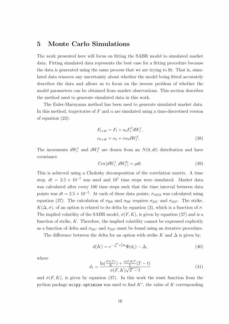
Table 2: Comparison of Monte Caro with equation (37).

β = 0 β = 1

K/F0 MC Eq. (37) MC Eq. (37)

0.9 0.07941 0.07900 0.08585 0.08637

1.0 0.05953 0.05953 0.07144 0.07147

1.1 0.07447 0.07711 0.08790 0.09034

5.2 Alternative Formulation

It will be shown in section 8 that q, defined in equation (65), can be viewed as a

single state variable for the SABR model. Therefore, as an alternative to simulating

equation (38), we can simulate q:

qt+dt = qt + vqtdW2t − (1− β)q2

t

(dW 1

t + vρdt− 1

2(2− β)qtdt

). (43)

17

Using this formulation σATM is calculated using equation (67). The calculation of σ25C

and σ25P remains an iterative procedure: a value of ψ must be found that satisfies

equation (61), where σ(ψ) is given by equation (66).

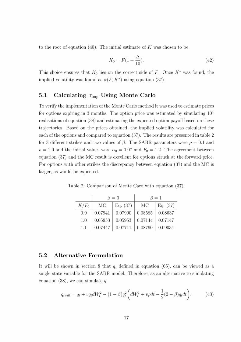
Figure 1 compares simulated values of σATM obtained by simulating equations (38)

and (43). On this scale, both methods appear to generate the same the trajectories

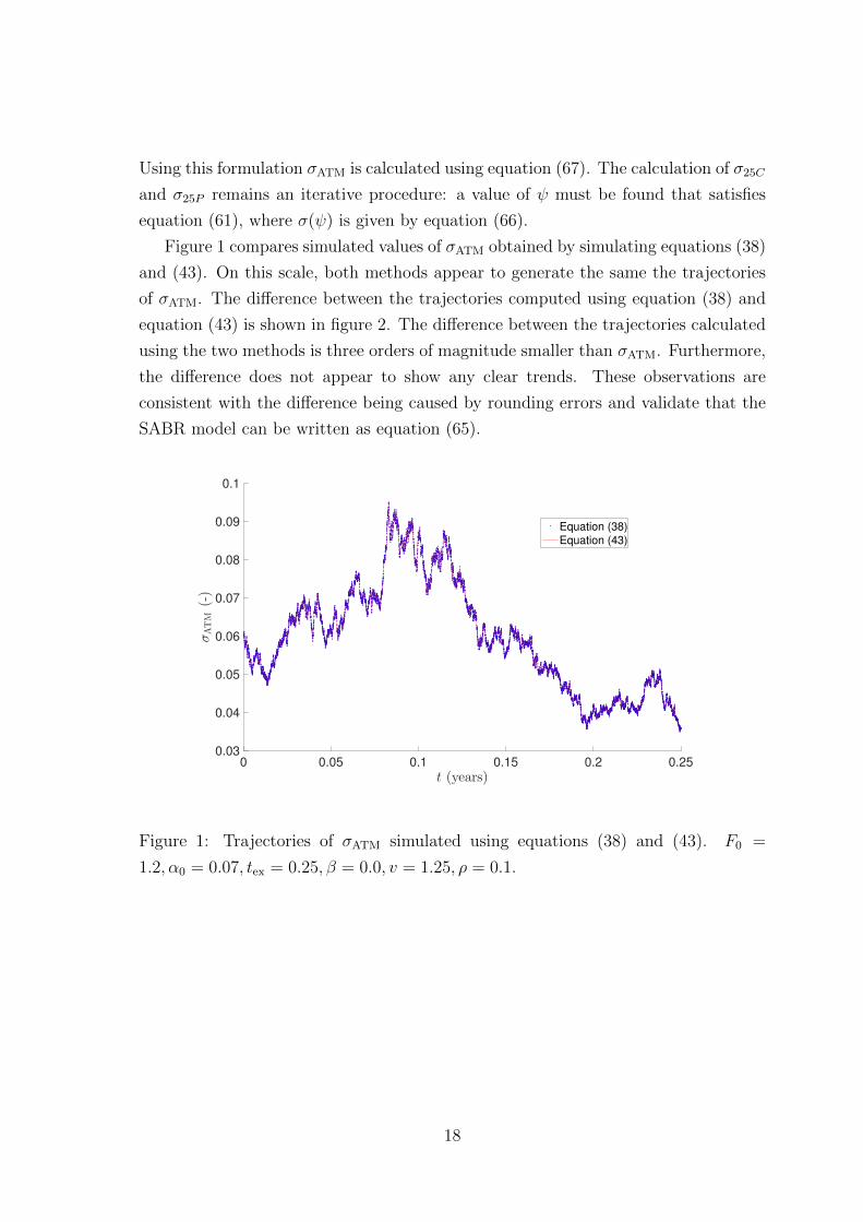
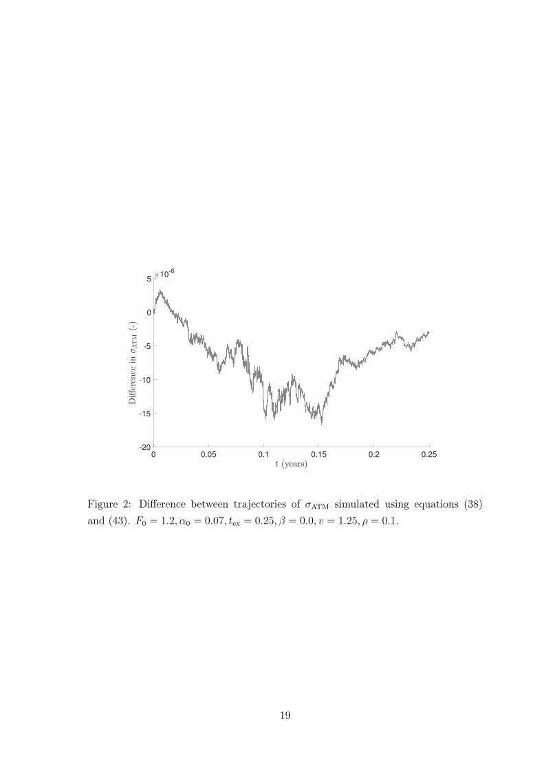
of σATM. The difference between the trajectories computed using equation (38) and

equation (43) is shown in figure 2. The difference between the trajectories calculated

using the two methods is three orders of magnitude smaller than σATM. Furthermore,

the difference does not appear to show any clear trends. These observations are

consistent with the difference being caused by rounding errors and validate that the

SABR model can be written as equation (65).

0 0.05 0.1 0.15 0.2 0.25

t (years)

0.03

0.04

0.05

0.06

0.07

0.08

0.09

0.1

σATM

(-)

Equation (38)

Equation (43)

Figure 1: Trajectories of σATM simulated using equations (38) and (43). F0 =

1.2, α0 = 0.07, tex = 0.25, β = 0.0, v = 1.25, ρ = 0.1.

18

0 0.05 0.1 0.15 0.2 0.25

t (years)

-20

-15

-10

-5

0

5

Difference

inσATM

(-)

×10-6

Figure 2: Difference between trajectories of σATM simulated using equations (38)

and (43). F0 = 1.2, α0 = 0.07, tex = 0.25, β = 0.0, v = 1.25, ρ = 0.1.

19

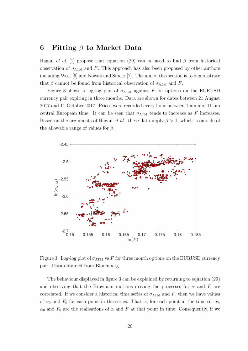
6 Fitting β to Market Data

Hagan et al. [1] propose that equation (29) can be used to find β from historical

observation of σATM and F . This approach has also been proposed by other authors

including West [6] and Nowak and Sibetz [7]. The aim of this section is to demonstrate

that β cannot be found from historical observation of σATM and F .

Figure 3 shows a log-log plot of σATM against F for options on the EURUSD

currency pair expiring in three months. Data are shown for dates between 21 August

2017 and 11 October 2017. Prices were recorded every hour between 1 am and 11 pm

central European time. It can be seen that σATM tends to increase as F increases.

Based on the arguments of Hagan et al., these data imply β > 1, which is outside of

the allowable range of values for β.

0.15 0.155 0.16 0.165 0.17 0.175 0.18 0.185

ln(F )

-2.7

-2.65

-2.6

-2.55

-2.5

-2.45

ln(σ

ATM)

Figure 3: Log-log plot of σATM vs F for three month options on the EURUSD currency

pair. Data obtained from Bloomberg.

The behaviour displayed in figure 3 can be explained by returning to equation (29)

and observing that the Brownian motions driving the processes for α and F are

correlated. If we consider a historical time series of σATM and F , then we have values

of α0 and F0 for each point in the series. That is, for each point in the time series,

α0 and F0 are the realisations of α and F at that point in time. Consequently, if we

20

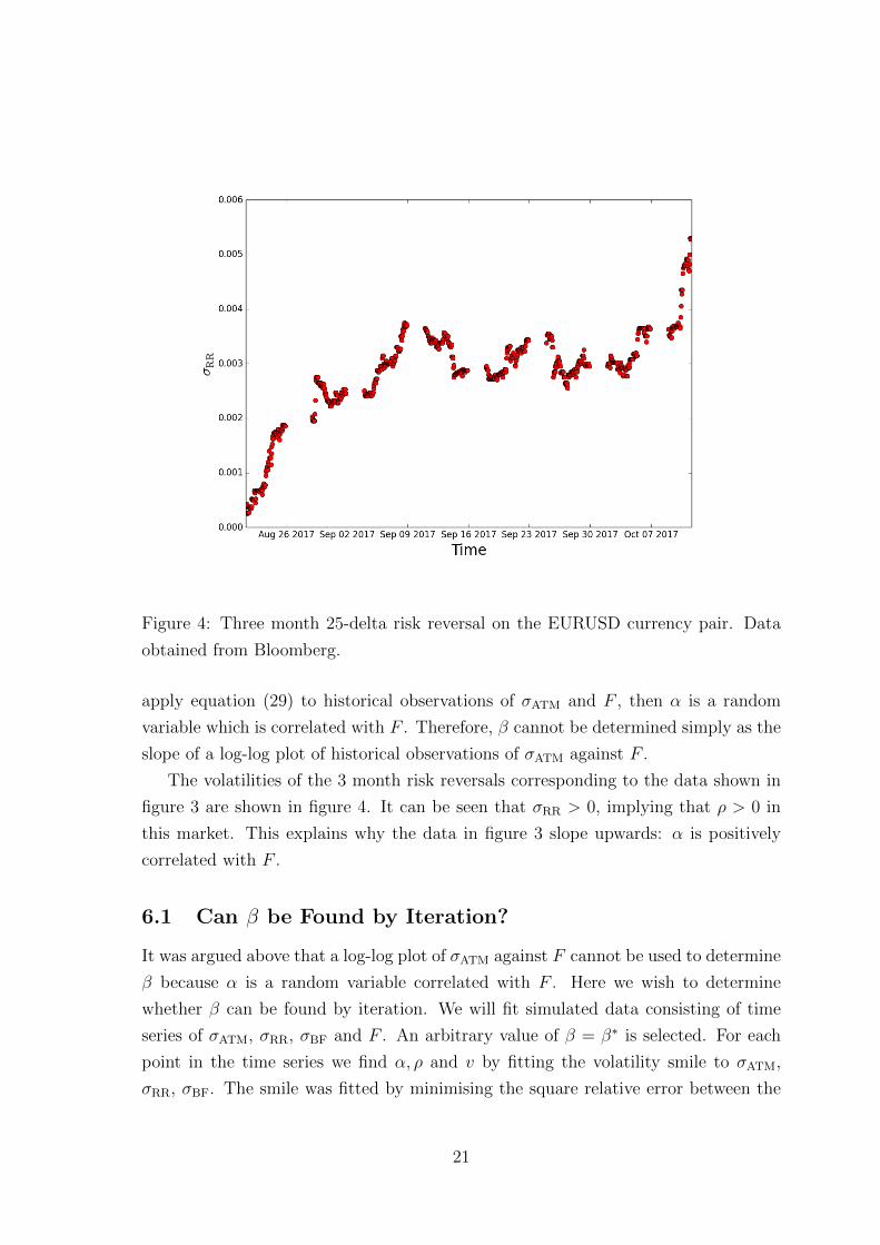
Figure 4: Three month 25-delta risk reversal on the EURUSD currency pair. Data

obtained from Bloomberg.

apply equation (29) to historical observations of σATM and F , then α is a random

variable which is correlated with F . Therefore, β cannot be determined simply as the

slope of a log-log plot of historical observations of σATM against F .

The volatilities of the 3 month risk reversals corresponding to the data shown in

figure 3 are shown in figure 4. It can be seen that σRR > 0, implying that ρ > 0 in

this market. This explains why the data in figure 3 slope upwards: α is positively

correlated with F .

6.1 Can β be Found by Iteration?

It was argued above that a log-log plot of σATM against F cannot be used to determine

β because α is a random variable correlated with F . Here we wish to determine

whether β can be found by iteration. We will fit simulated data consisting of time

series of σATM, σRR, σBF and F . An arbitrary value of β = β∗ is selected. For each

point in the time series we find α, ρ and v by fitting the volatility smile to σATM,

σRR, σBF. The smile was fitted by minimising the square relative error between the

21

observed market quotes and the model predictions for these volatilities, i.e.

error(α, ρ, v) =(σ′ATM(α, β∗, ρ, v)

σATM

− 1)2

+(σ′RR(α, β∗, ρ, v)

σRR

− 1)2

+(σ′BF(α, β∗, ρ, v)

σBF

− 1)2

. (44)

Here the relative errors associated with each of the three volatility quotes are weighted

equally for simplicity. When fitting a volatility smile in practice it might be preferable

to weight the three errors differently. For example, more weighting might be given

to volatility quotes with a higher traded volume. Under normal circumstances this

would lead to a larger weighting for the error associated with σATM.

Having fitted the smile at each point in the time series, we have a (fitted) value of

α for each of these smiles. Using these values of α we can plot log(σATM/α) against

log(F ). From equation (29) the slope of this plot is β − 1. Therefore, we can update

our value of β∗ based on the slope of this plot. We aim to iterate in this manner until

the value of β stops changing between iterations.

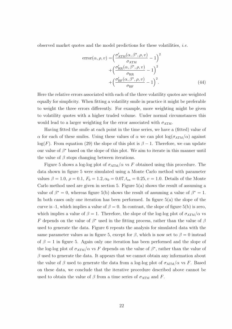
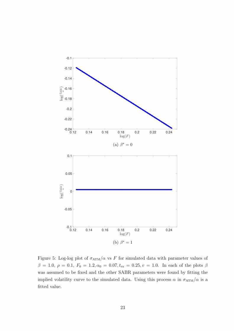
Figure 5 shows a log-log plot of σATM/α vs F obtained using this procedure. The

data shown in figure 5 were simulated using a Monte Carlo method with parameter

values β = 1.0, ρ = 0.1, F0 = 1.2, α0 = 0.07, tex = 0.25, v = 1.0. Details of the Monte

Carlo method used are given in section 5. Figure 5(a) shows the result of assuming a

value of β∗ = 0, whereas figure 5(b) shows the result of assuming a value of β∗ = 1.

In both cases only one iteration has been performed. In figure 5(a) the slope of the

curve is -1, which implies a value of β = 0. In contrast, the slope of figure 5(b) is zero,

which implies a value of β = 1. Therefore, the slope of the log-log plot of σATM/α vs

F depends on the value of β∗ used in the fitting process, rather than the value of β

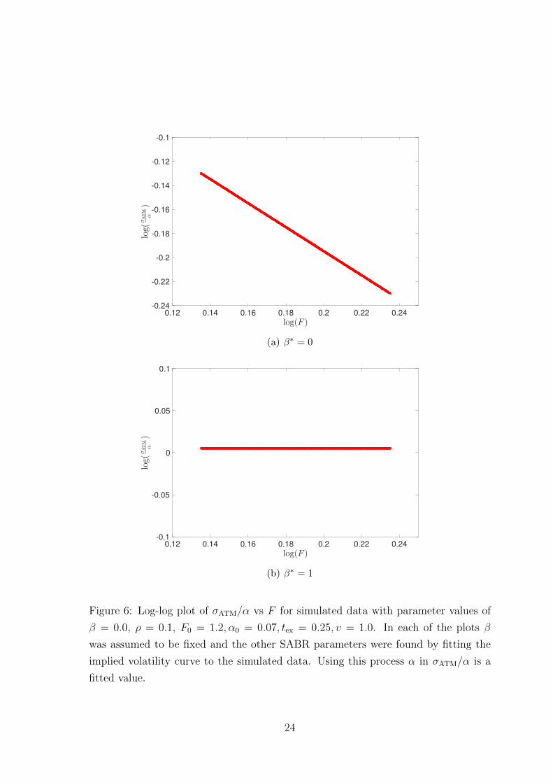
used to generate the data. Figure 6 repeats the analysis for simulated data with the

same parameter values as in figure 5, except for β, which is now set to β = 0 instead

of β = 1 in figure 5. Again only one iteration has been performed and the slope of

the log-log plot of σATM/α vs F depends on the value of β∗, rather than the value of

β used to generate the data. It appears that we cannot obtain any information about

the value of β used to generate the data from a log-log plot of σATM/α vs F . Based

on these data, we conclude that the iterative procedure described above cannot be

used to obtain the value of β from a time series of σATM and F .

22

0.12 0.14 0.16 0.18 0.2 0.22 0.24

log(F )

-0.24

-0.22

-0.2

-0.18

-0.16

-0.14

-0.12

-0.1log(

σATM

α)

(a) β∗ = 0

0.12 0.14 0.16 0.18 0.2 0.22 0.24

log(F )

-0.1

-0.05

0

0.05

0.1

log(

σATM

α)

(b) β∗ = 1

Figure 5: Log-log plot of σATM/α vs F for simulated data with parameter values of

β = 1.0, ρ = 0.1, F0 = 1.2, α0 = 0.07, tex = 0.25, v = 1.0. In each of the plots β

was assumed to be fixed and the other SABR parameters were found by fitting the

implied volatility curve to the simulated data. Using this process α in σATM/α is a

fitted value.

23

0.12 0.14 0.16 0.18 0.2 0.22 0.24

log(F )

-0.24

-0.22

-0.2

-0.18

-0.16

-0.14

-0.12

-0.1log(

σATM

α)

(a) β∗ = 0

0.12 0.14 0.16 0.18 0.2 0.22 0.24

log(F )

-0.1

-0.05

0

0.05

0.1

log(

σATM

α)

(b) β∗ = 1

Figure 6: Log-log plot of σATM/α vs F for simulated data with parameter values of

β = 0.0, ρ = 0.1, F0 = 1.2, α0 = 0.07, tex = 0.25, v = 1.0. In each of the plots β

was assumed to be fixed and the other SABR parameters were found by fitting the

implied volatility curve to the simulated data. Using this process α in σATM/α is a

fitted value.

24

7 Fitting Using Variance-Covariance Matching

In this section we examine whether the SABR parameters can be obtained by match-

ing the variance and covariance of the Brownian motions to the time series of σATM

and F . This method is considered as an alternative to the approach described in

section 6. We can rearrange equation (23) to give the following expressions for dW 1

and dW 2

dW 1 =dF

αF β, (45)

dW 2 =dα

vα.

Discretising equation (45) gives

dW 1 ≈ Ft+dt − FtαtF

βt

, (46)

dW 2 ≈ αt+dt − αtvαt

.

For given values of β, ρ and v, α can be calculated from σATM and F using equa-

tion (28). Consider the problem of fitting the SABR model to market data. We

observe time series of σATM and F in the market. From these data we can calculate

dW 1(β, ρ, v) and dW 2(β, ρ, v) using equations (28) and (46).

Since W 1 and W 2 are correlated Brownian motions, we can write the following

V(dW 1) = dt, (47)

V(dW 2) = dt,

Cov(dW 1, dW 2) = ρdt.

Therefore, one approach to fitting the model is to select values of β, ρ and v which

cause the sample variances and covariance of dW 1 and dW 2 to be equal to those given

in equation (47). That is, we seek β, ρ and v such that the following conditions are

met

V(Ft+dt − FtαtF

βt

√dt

) = 1, (48)

V(αt+dt − αtvαt√dt

) = 1,

Cov(Ft+dt − FtαtF

βt

√dt,αt+dt − αtvαt√dt

) = ρ.

25

We apply variance-covariance matching to simulated data with β = 1.0, ρ = 0.1,

F0 = 1.2, α0 = 0.07, tex = 0.25 and v = 1.0. The simulated data consists of time series

of σATM and F with 105 observations of each. The time step between the observations

is dt = 2.5× 10−5 years. Fitting is performed by minimising the sum of the relative

errors

error(β, ρ, v) =

∣∣∣∣V(Ft+dt − FtαtF

βt

√dt

)− 1

∣∣∣∣+

∣∣∣∣V(αt+dt − αtvαt√dt

)− 1

∣∣∣∣ (49)

+

∣∣∣∣ ρ

Cov(Ft+dt−FtαtF

βt

√dt, αt+dt−αtvαt√dt

)− 1

∣∣∣∣. (50)

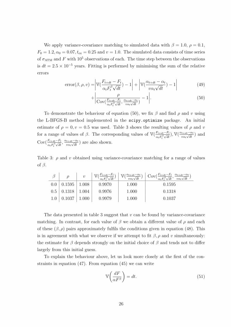
To demonstrate the behaviour of equation (50), we fix β and find ρ and v using

the L-BFGS-B method implemented in the scipy.optimize package. An initial

estimate of ρ = 0, v = 0.5 was used. Table 3 shows the resulting values of ρ and v

for a range of values of β. The corresponding values of V(Ft+dt−FtαtF

βt

√dt

),V(αt+dt−αtvαt√dt

) and

Cov(Ft+dt−FtαtF

βt

√dt, αt+dt−αtvαt√dt

) are also shown.

Table 3: ρ and v obtained using variance-covariance matching for a range of values

of β.

β ρ v V(Ft+dt−FtαtF

βt

√dt

) V(αt+dt−αtvαt√dt

) Cov(Ft+dt−FtαtF

βt

√dt, αt+dt−αtvαt√dt

)

0.0 0.1595 1.008 0.9970 1.000 0.1595

0.5 0.1318 1.004 0.9976 1.000 0.1318

1.0 0.1037 1.000 0.9979 1.000 0.1037

The data presented in table 3 suggest that v can be found by variance-covariance

matching. In contrast, for each value of β we obtain a different value of ρ and each

of these (β, ρ) pairs approximately fulfils the conditions given in equation (48). This

is in agreement with what we observe if we attempt to fit β, ρ and v simultaneously:

the estimate for β depends strongly on the initial choice of β and tends not to differ

largely from this initial guess.

To explain the behaviour above, let us look more closely at the first of the con-

straints in equation (47). From equation (45) we can write

V(dF

αF β

)= dt. (51)

26

Using equation (28) and noting that the (T − t) term is typically small, we estimate

α as

α ≈ σATMF1−β. (52)

Combining equations (51) and (52) gives

V(

dF

σATMF

)= dt, (53)

which is independent of β, ρ and v. Hence, β, ρ and v only enter equation (51) through

the (T − t) term, which is normally less than 1 or 2%.

To summarise, although this approach seems promising because we have three

constraints for three unknowns (β, ρ and v), it is difficult to determine the three

unknowns uniquely because one of the constraints is relatively insensitive to the three

unknowns.

27

8 Relationship Between σATM, σRR and σBF

In the FX market the volatility smile is described by three main volatility quotes:

σATM, σRR and σBF. The definitions of these can be found in section 2. Of these three

main volatilities, σATM is the most liquid contract and might, therefore, be expected

to be more up to date than σRR or σBF. Hence, one motivation for fitting a model

to the FX volatility smile is to predict price changes for the less liquid σRR and σBF

contracts based on observed changes in σATM. To this end, this section focuses on the

relationship between σATM, σRR and σBF predicted by the SABR model.

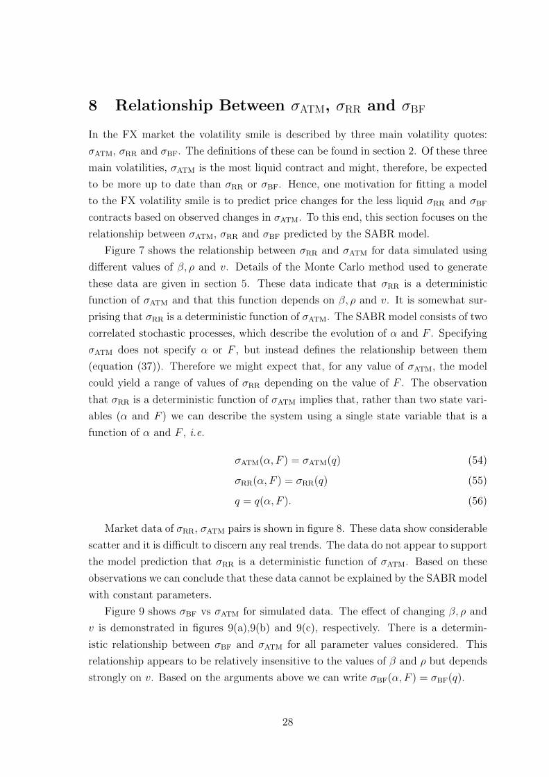
Figure 7 shows the relationship between σRR and σATM for data simulated using

different values of β, ρ and v. Details of the Monte Carlo method used to generate

these data are given in section 5. These data indicate that σRR is a deterministic

function of σATM and that this function depends on β, ρ and v. It is somewhat sur-

prising that σRR is a deterministic function of σATM. The SABR model consists of two

correlated stochastic processes, which describe the evolution of α and F . Specifying

σATM does not specify α or F , but instead defines the relationship between them

(equation (37)). Therefore we might expect that, for any value of σATM, the model

could yield a range of values of σRR depending on the value of F . The observation

that σRR is a deterministic function of σATM implies that, rather than two state vari-

ables (α and F ) we can describe the system using a single state variable that is a

function of α and F , i.e.

σATM(α, F ) = σATM(q) (54)

σRR(α, F ) = σRR(q) (55)

q = q(α, F ). (56)

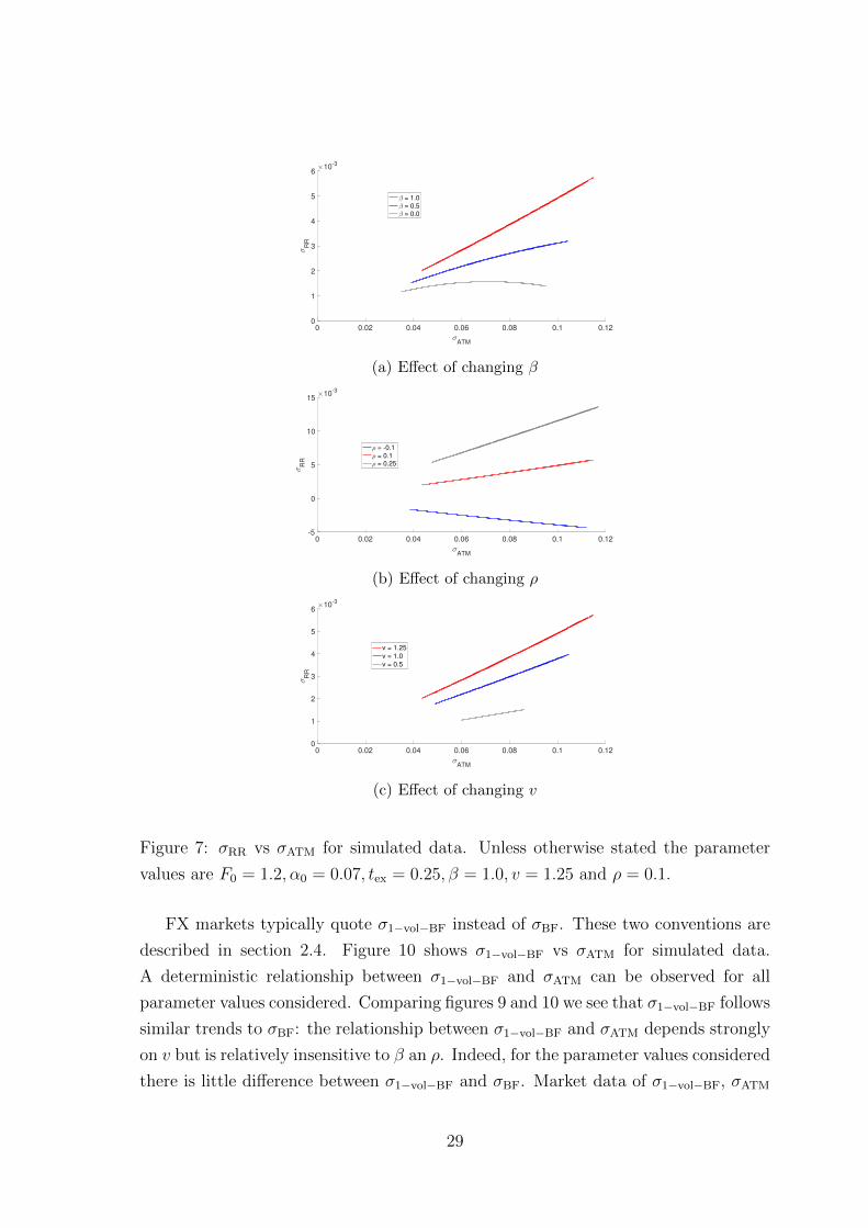
Market data of σRR, σATM pairs is shown in figure 8. These data show considerable

scatter and it is difficult to discern any real trends. The data do not appear to support

the model prediction that σRR is a deterministic function of σATM. Based on these

observations we can conclude that these data cannot be explained by the SABR model

with constant parameters.

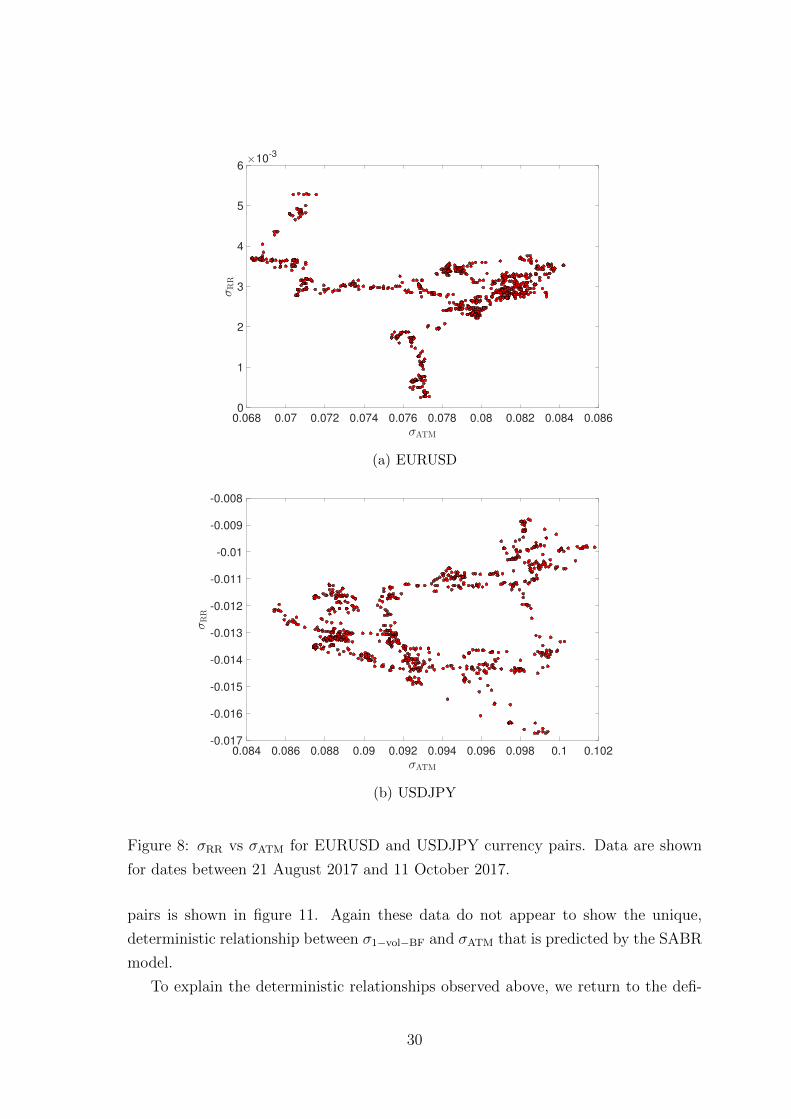
Figure 9 shows σBF vs σATM for simulated data. The effect of changing β, ρ and

v is demonstrated in figures 9(a),9(b) and 9(c), respectively. There is a determin-

istic relationship between σBF and σATM for all parameter values considered. This

relationship appears to be relatively insensitive to the values of β and ρ but depends

strongly on v. Based on the arguments above we can write σBF(α, F ) = σBF(q).

28

0 0.02 0.04 0.06 0.08 0.1 0.12

σATM

0

1

2

3

4

5

6

σR

R

×10-3

β = 1.0

β = 0.5

β = 0.0

(a) Effect of changing β

0 0.02 0.04 0.06 0.08 0.1 0.12

σATM

-5

0

5

10

15

σR

R

×10-3

ρ = -0.1

ρ = 0.1

ρ = 0.25

(b) Effect of changing ρ

0 0.02 0.04 0.06 0.08 0.1 0.12

σATM

0

1

2

3

4

5

6

σR

R

×10-3

v = 1.25

v = 1.0

v = 0.5

(c) Effect of changing v

Figure 7: σRR vs σATM for simulated data. Unless otherwise stated the parameter

values are F0 = 1.2, α0 = 0.07, tex = 0.25, β = 1.0, v = 1.25 and ρ = 0.1.

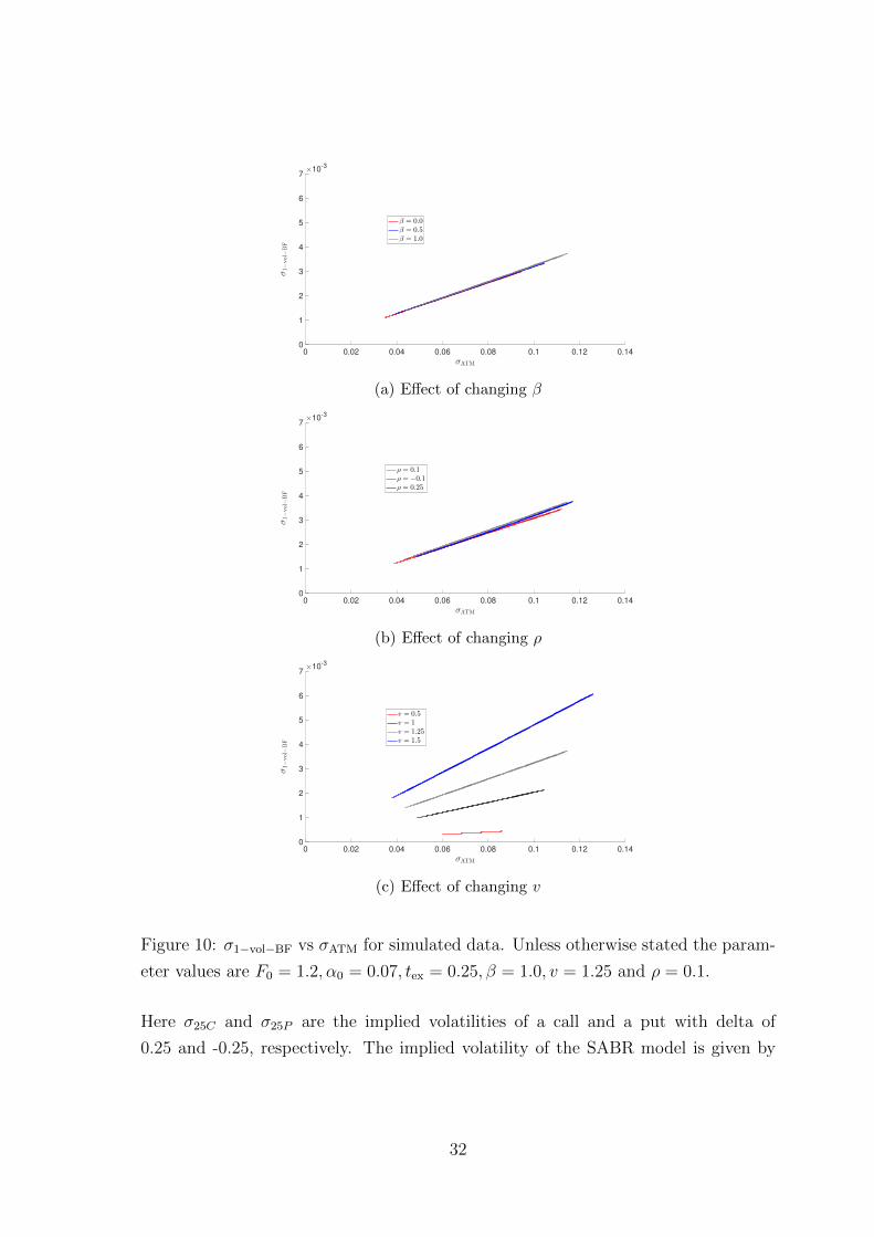
FX markets typically quote σ1−vol−BF instead of σBF. These two conventions are

described in section 2.4. Figure 10 shows σ1−vol−BF vs σATM for simulated data.

A deterministic relationship between σ1−vol−BF and σATM can be observed for all

parameter values considered. Comparing figures 9 and 10 we see that σ1−vol−BF follows

similar trends to σBF: the relationship between σ1−vol−BF and σATM depends strongly

on v but is relatively insensitive to β an ρ. Indeed, for the parameter values considered

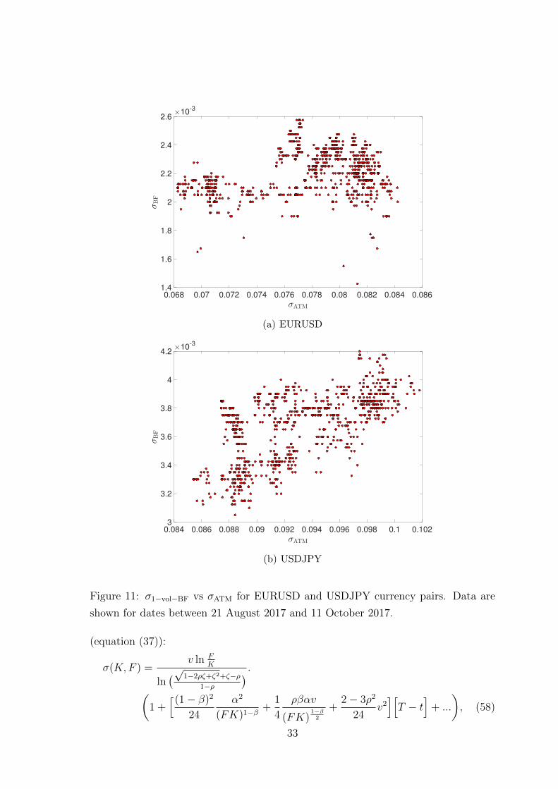
there is little difference between σ1−vol−BF and σBF. Market data of σ1−vol−BF, σATM

29

0.068 0.07 0.072 0.074 0.076 0.078 0.08 0.082 0.084 0.086

σATM

0

1

2

3

4

5

6

σRR

×10-3

(a) EURUSD

0.084 0.086 0.088 0.09 0.092 0.094 0.096 0.098 0.1 0.102

σATM

-0.017

-0.016

-0.015

-0.014

-0.013

-0.012

-0.011

-0.01

-0.009

-0.008

σRR

(b) USDJPY

Figure 8: σRR vs σATM for EURUSD and USDJPY currency pairs. Data are shown

for dates between 21 August 2017 and 11 October 2017.

pairs is shown in figure 11. Again these data do not appear to show the unique,

deterministic relationship between σ1−vol−BF and σATM that is predicted by the SABR

model.

To explain the deterministic relationships observed above, we return to the defi-

30

0 0.02 0.04 0.06 0.08 0.1 0.12 0.14

σATM

0

1

2

3

4

5

6

7

σBF

×10-3

β = 0.0

β = 0.5

β = 1.0

(a) Effect of changing β

0 0.02 0.04 0.06 0.08 0.1 0.12 0.14

σATM

0

1

2

3

4

5

6

7

σBF

×10-3

ρ = 0.1

ρ = −0.1

ρ = 0.25

(b) Effect of changing ρ

0 0.02 0.04 0.06 0.08 0.1 0.12 0.14

σATM

0

1

2

3

4

5

6

7

σBF

×10-3

v = 0.5

v = 1

v = 1.25

v = 1.5

(c) Effect of changing v

Figure 9: σBF vs σATM for simulated data. Unless otherwise stated the parameter

values are F0 = 1.2, α0 = 0.07, tex = 0.25, β = 1.0, v = 1.25 and ρ = 0.1.

nitions of σRR and σBF. Equations (7) and (8) are repeated here for convenience.

σ25RR(t, T ) = σ25C(t, T )− σ25P (t, T ),

σ25BF(t, T ) =1

2

[σ25C(t, T ) + σ25P (t, T )

]− σATM(t, T ). (57)

31

0 0.02 0.04 0.06 0.08 0.1 0.12 0.14

σATM

0

1

2

3

4

5

6

7

σ1−vol−

BF

×10-3

β = 0.0

β = 0.5

β = 1.0

(a) Effect of changing β

0 0.02 0.04 0.06 0.08 0.1 0.12 0.14

σATM

0

1

2

3

4

5

6

7

σ1−vol−

BF

×10-3

ρ = 0.1

ρ = −0.1

ρ = 0.25

(b) Effect of changing ρ

0 0.02 0.04 0.06 0.08 0.1 0.12 0.14

σATM

0

1

2

3

4

5

6

7

σ1−vol−

BF

×10-3

v = 0.5

v = 1

v = 1.25

v = 1.5

(c) Effect of changing v

Figure 10: σ1−vol−BF vs σATM for simulated data. Unless otherwise stated the param-

eter values are F0 = 1.2, α0 = 0.07, tex = 0.25, β = 1.0, v = 1.25 and ρ = 0.1.

Here σ25C and σ25P are the implied volatilities of a call and a put with delta of

0.25 and -0.25, respectively. The implied volatility of the SABR model is given by

32

0.068 0.07 0.072 0.074 0.076 0.078 0.08 0.082 0.084 0.086

σATM

1.4

1.6

1.8

2

2.2

2.4

2.6

σBF

×10-3

(a) EURUSD

0.084 0.086 0.088 0.09 0.092 0.094 0.096 0.098 0.1 0.102

σATM

3

3.2

3.4

3.6

3.8

4

4.2

σBF

×10-3

(b) USDJPY

Figure 11: σ1−vol−BF vs σATM for EURUSD and USDJPY currency pairs. Data are

shown for dates between 21 August 2017 and 11 October 2017.

(equation (37)):

σ(K,F ) =v ln F

K

ln(√1−2ρζ+ζ2+ζ−ρ

1−ρ

) .(1 +

[(1− β)2

24

α2

(FK)1−β +1

4

ρβαv

(FK)1−β2

+2− 3ρ2

24v2][T − t

]+ ...

), (58)

33

where

ζ =v

α

F 1−β −K1−β

1− β. (59)

FX options are quoted in terms of delta, ∆, and we wish to determine σ25C and σ25P .

Adopting this convention, we can write

ln

(F

K

)= wσ

√τΦ−1(|∆|)− σ2τ

2, (60)

where w is 1 for a call and -1 for a put. Define

ψ = wσ√τΦ−1(|∆|)− σ2τ

2. (61)

Then

ln

(F

K

)= ψ, (62)

and

FK = F 2 exp (−ψ). (63)

We can rewrite ζ as

ζ =v

αF (1−β) 1− exp (−ψ(1− β))

1− β

=v

q

1− exp (−ψ(1− β))

1− β, (64)

where

q =α

F 1−β . (65)

Writing equation (37) in this notation gives

σ(ψ) =vψ

ln(√

1−2ρζ+ζ2+ζ−ρ1−ρ

) .(

1 +[(1− β)2

24q2eψ(1−β) +

ρβqv

4eψ(1−β)

2 +2− 3ρ2

24v2][T − t

]+ ...

). (66)

Note that neither α nor F appear explicitly in equation (66) and that ψ depends on

σ(ψ), so equation (66) is not an explicit equation for σ(ψ). For the case of options

written at-the-money we have

σATM = σ(0)

=α

F 1−β

(1 +

[(1− β)2

24

α2

F 2−2β+

1

4

ρβαv

F 1−β +2− 3ρ2

24v2][T − t

]+ ...

)= q

(1 +

[(1− β)2

24q2 +

ρβqv

4+

2− 3ρ2

24v2][T − t

]+ ...

). (67)

34

Based on equation (66) it would be possible to calculate σRR and σBF if the SABR

parameters (β, ρ, v) and q are known. Since (67) is a special case of (66), σATM is also

uniquely determined by β, ρ, v and q. Therefore, for specified values of β, ρ and v,

there is a fixed, deterministic relationship between σATM, σRR and σBF. This explains

the behaviour shown in figures 7 and 9.

Let us take stock of the above: if we consider the volatility smile as a mapping

between ∆ and σimp, then this mapping depends on the SABR parameters ρ, β, v

and on q. For a fixed model (i.e. specified values of ρ, β and v), the state of the

system can be described by q alone. Note that we have reduced the number of SABR

parameters by one: α is no longer considered a parameter to be fitted. We have

also reduced by one the number of variables that we can observe: we are no longer

interested in observing the forward price, F . Motivated by the above, let us consider

the SDE for q as defined in equation (65). Applying Ito’s Lemma

dq = −α(1− β)dF

F 2−β +dα

F 1−β +1

2α(1− β)(2− β)

dF 2

F 3−β −1− βF 2−β dFdα

= −(1− β)q2dW1 + vqdW2 +1

2(1− β)(2− β)q3dt− (1− β)vq2ρdt. (68)

Therefore, it should be possible to describe the evolution of the volatility smile using

equation (68). It is also noted that q is the instantaneous Black Scholes volatility. To

see this, we rewrite equation (23) as

dF =α

F 1−βFdW1 (69)

and compare equation (69) to the Black-Scholes model for the asset price

dF = σBSFdW1. (70)

Comparing equation (69) and (70) we obtain the instantaneous relation

σBS =α

F 1−β = q. (71)

It is also interesting to note that q ≈ σATM. Equation (67) shows that q differs from

σATM by a factor of 1+( (1−β)2

24q2+ ρβqv

4+ 2−3ρ2

24v2)(T−t). It was shown in section 3 that

the (T − t) term is usually less than 1 or 2% for a typical volatility smile. Therefore

the discprenacy between q and σATM will usually be of this order of magnitude.

35

9 Covariance Between dq and dF

In this section we examine the covariance between dq and dF . We noted in section 8

that q ≈ σATM. Therefore, we can view Cov(dq, dF ) as a proxy for Cov(dσATM, dF ).

Cov(dσATM, dF ) is an important quantity because it allows us to relate a change in F

to a change in σATM. This relation is valuable because it allows vega exposure, which

is expensive to hedge, to be partially hedged with delta, which is cheap to hedge.

In section 8 we saw that

dq = −(1− β)q2dW1 + vqdW2 +1

2(1− β)(2− β)q3dt− (1− β)vq2ρdt, (72)

and

dF = αF βdW 1. (73)

By direct computation we can calculate the covariance between dq and dF :

Cov(dq, dF ) = E(dqdF )

= dt(ρvE(q2F )− (1− β)E(q3F )). (74)

We can also consider the variance of dq

V(dq) =

((1− β)2E(q4) + v2E(q2)− 2vρ(1− β)E(q3)

)dt. (75)

However, for common parameter values this is dominated by v2E(q2) and so provides

little information regarding β or ρ. We could estimate v as

v ≈

√V(dq)

E(q2)dt. (76)

The variance of dF is

V(dF ) = E(α2F 2β)dt

= E(q2F 2)dt (77)

The correlation between dq and dF is

ρdq,dF =Cov(dq, dF )√V(dq)V(dF )

=ρvE(q2F )− (1− β)E(q3F )√

E(q2F 2)√

(1− β)2E(q4) + v2E(q2)− 2vρ(1− β)E(q3)

≈ ρvE(q2F )− (1− β)E(q3F )√E(q2F 2)v

√E(q2)

(78)

36

If we consider the instantaneous correlation, such that q and F are known, then

ρdq,dF ≈ ρ− (1− β)q

v. (79)

It was noted in the literature survey that a volatility smile can be equally well

described with any value of β. It is interesting to examine the behaviour of equa-

tion (79) for these different fits. Consider the volatility smile in table 4, which was

generated using β = 1, ρ = 0.1 and v = 1.0. Table 5 shows the SABR parameters

Table 4: Sample volatility smile data.

F σATM σRR σBF

1.2 7.17 % 0.256 % 0.146 %

fitted to these volatilities for a range of values of β. For each of these parameter sets,

the value of ρdq,dF estimated from equation (79) is also given. These data illustrate

that the instantaneous correlation between dq and dF is insensitive to the choice of

β.

Table 5: SABR parameters fitted to the data in table 4 for a range of values of β.

β ρ v q ρdq,dF

0.0 0.1668 1.013 0.06699 0.1007

0.2 0.1537 1.010 0.06699 0.1006

0.4 0.1404 1.007 0.06698 0.1005

0.6 0.1270 1.005 0.06697 0.1003

0.8 0.1135 1.002 0.06697 0.1001

1.0 0.1000 1.000 0.06697 0.1000

The data shown in table 4 are characteristic of a currency pair with a small risk

reversal (such as EURUSD). We now repeat the analysis for the data shown in table 6.

These data represent a currency pair with a large risk reversal; for example, USDJPY.

Table 7 shows the SABR parameters fitted to the volatilities in table 6 for a range

of values of β. In this case the difference between the largest and smallest values

of ρdq,dF is larger, but still less than 2%. Based on the analysis above, it can be

concluded that ρdq,dF is insensitive to the choice of β. This is unsurprising: ρdq,dF is

related to the shape of the volatility smile and it is known that smiles can be well

fitted by the SABR model for any value of β [12].

37

Table 6: Sample volatility smile for a currency pair with a large risk reversal.

F σATM σRR σBF

100 9.225 % -1.475 % 0.3475 %

Table 7: SABR parameters fitted to the data in table 6 for a range of values of β.

β ρ v q ρdq,dF

0.0 -0.26984092 1.36912134 0.08909337 -0.3349

0.2 -0.28201586 1.37765979 0.08913005 -0.3338

0.4 -0.29400046 1.38646149 0.08917033 -0.3326

0.6 -0.30579258 1.39552372 0.08921424 -0.3314

0.8 -0.31739115 1.40484087 0.0892618 -0.3301

1.0 -0.32879486 1.41441135 0.08931306 -0.3288

9.1 Does the Choice of β Matter?

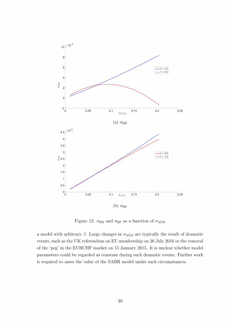
Figure 12 shows σRR and σBF as a function of σATM for the parameter values shown

in table 5 (β = 0.0 and β = 1.0). From figure 12(b) it can be observed that the choice

of β has little effect on the relationship between σBF and σATM. In contrast, the

relationship between σRR and σATM depends strongly on β. Figure 12(a) shows the

relationship between σRR and σATM for β = 0.0 and β = 1.0. The two curves intersect

at σATM ≈ 0.07, which is the point to which the model was fitted, but diverge either

side of this point.

Based on the results in figure 12 we can conclude that fitting β correctly would be

critical if we wanted to have a model with constant parameter values that is capable

of describing the relationship between σRR and σATM over a wide range of σATM. It

is, however, valid to ask whether such a model offers significant real world advantages

over a model with an arbitrary choice of β that is recalibrated frequently. If σATM

evolves slowly, then recalibrating the arbitrary β model on a regular basis would

ensure that the model’s prediction for σRR would always be close to the true value.

Under these conditions the advantage of correctly determining β is that the model

would not need to be recalibrated as frequently.

On the other hand, if we observe a step change in σATM then a model with the

correct value of β would be expected to yield a more accurate prediction of σRR than

38

0 0.05 0.1 0.15 0.2 0.25σATM

-2

0

2

4

6

8

10

σRR

×10-3

β = 1.0

β = 0.0

(a) σRR

0 0.05 0.1 0.15 0.2 0.25σATM

0

0.5

1

1.5

2

2.5

3

3.5

4

4.5

σBF

×10-3

β = 0.0

β = 1.0

(b) σBF

Figure 12: σRR and σBF as a function of σATM

a model with arbitrary β. Large changes in σATM are typically the result of dramatic

events, such as the UK referendum on EU membership on 26 July 2016 or the removal

of the ‘peg’ in the EURCHF market on 15 January 2015. It is unclear whether model

parameters could be regarded as constant during such dramatic events. Further work

is required to asses the value of the SABR model under such circumstances.

39

10 Fitting the SABR Model

In this section we propose a new method for fitting the SABR model to observed

FX market data. After describing the method, we demonstrate its behaviour in the

idealised case of fitting data generated using the SABR model. Thereafter the effect

of noise on the fitting accuracy is examined. We isolate the effect of noise on each of

the three volatility quotes σATM, σRR and σBF. Finally conclusions are drawn.

The deterministic nature of the relationships between σATM, σRR and σBF and the

dependence of these relationships on the SABR parameters suggests that it should

be possible to fit the SABR model to market data using observations of the triplet

[σATM, σRR, σBF]. It was argued in section 8 that, in an FX setting, the SABR model

can be regarded as having a single state variable, q. Equation (67) relates σATM to q

and the model parameters. Therefore, q and σATM are interchangeable and the state

of the system is fully described by σATM. From a practical point of view we prefer to

work with σATM because, unlike q, it can be observed directly in the market.

If we regard σATM as a state variable, then the [σATM, σRR, σBF] triplet provides

us with two constraints: namely that the model predictions for σRR and σBF should

match the observed values. The model has three unknown parameters (β, ρ and v)

so one triplet will generally not contain sufficient information to fit the model. One

approach to fitting the model would be to consider n triplets. The parameter values

would then be found by minimising the error between the predicted and observed

values of σRR and σBF. For example

error(β, ρ, v) =n∑i

[(σ′RR(β, ρ, v)

σRR

− 1)2

+(σ′BF(β, ρ, v)

σBF

− 1)2]

(80)

where σ′RR(β, ρ, v) and σ′BF(β, ρ, v) are, respectively, the risk reversal and butterfly

spread predicted by the SABR model. In equation (80) relative errors were used to

account for possible differences in the magnitudes of σRR and σBF. In the case that

σRR is very small, absolute errors could be used to prevent division by zero.

Equation (80) is minimised subject to the following bounds on β, ρ and v:

0 ≤ β ≤ 1

−0.9 ≤ ρ ≤ 0.9

0 ≤ v ≤ 100.

The bounds on β are specified by the SABR model. β = 0 gives arithmetic Brownian

motion, while β = 1 results in geometric Brownian motion. In principle ρ can take

40

any value between -1 and 1. We prefer tighter bounds on ρ to prevent division by zero

during the minimisation. The lower bound on v is applied because v is a volatility. An

upper bound of v = 100 is applied to prevent the numerical optimiser from venturing

into regions with a very large v. The typical magnitude value of v is v ≈ 1. The upper

bound is sufficiently far from this value that v can be considered as being essentially

unbounded from above. The initial estimate of the parameter values is chosen to be

β∗ = 0.5, ρ∗ = 0.0, v∗ = 0.5. Constrained minimisation is performed in python using

the L-BFGS-B method implemented in the scipy.optimize package. Python code

developed during this project to fit the SABR model using the method described

above can be found in appendix A.

10.1 Fitting in the Absence of Noise

To demonstrate the behaviour of the fitting procedure described above we apply it to

fictitious data with known values of β, ρ and v. It was argued above that σATM can

be regarded as a state variable for the system. Therefore, we can generate sample

data simply by specifying values of σATM. Table 8 shows the data to be fitted. We

consider the case of n = 2, i.e. two data points are used to fit the model. In all cases

point 1, corresponding to σATM = 0.06 is used in the fit. The second point is varied

to show the effect of the range of σATM on the fitting quality. Define the error in the

model fitting as the difference between the true model parameters and those found

by fitting the model to the data:

h =

(β′ − β

)2

+

(ρ′

ρ− 1

)2

+

(v′

v− 1

)2

. (81)

Here β′, ρ′ and v′ are the parameter values found by fitting the model. The absolute

error was chosen for β to avoid division by zero.

Figure 13(a) shows the fitting error as a function of the range of σATM. It can

be seen that the fitting error tends to decrease as the range of σATM is increased

and that, for all values of β, the fitting error is very small when the range of σATM

is 0.01 or larger. In all cases considered the fitting error is smaller than 10−5 when

range of σATM is 0.01 or larger. For β = 0.5 the fitting error is small for all values

of the range of σATM. This may be due to the initial estimate of β, β∗ = 0.5, used

in the fitting procedure. Figure 13(b) shows the fitting error as a function of the

range of σATM when the initial estimate of the parameter values is chosen to be

β∗ = 0.0, ρ∗ = 0.0, v∗ = 0.5. This choice leads to a small fitting error for β = 0.0 for

41

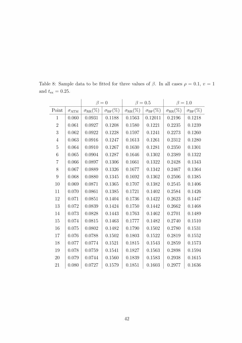
Table 8: Sample data to be fitted for three values of β. In all cases ρ = 0.1, v = 1

and tex = 0.25.

β = 0 β = 0.5 β = 1.0

Point σATM σRR(%) σBF(%) σRR(%) σBF(%) σRR(%) σBF(%)

1 0.060 0.0931 0.1188 0.1563 0.12011 0.2196 0.1218

2 0.061 0.0927 0.1208 0.1580 0.1221 0.2235 0.1239

3 0.062 0.0922 0.1228 0.1597 0.1241 0.2273 0.1260

4 0.063 0.0916 0.1247 0.1613 0.1261 0.2312 0.1280

5 0.064 0.0910 0.1267 0.1630 0.1281 0.2350 0.1301

6 0.065 0.0904 0.1287 0.1646 0.1302 0.2389 0.1322

7 0.066 0.0897 0.1306 0.1661 0.1322 0.2428 0.1343

8 0.067 0.0889 0.1326 0.1677 0.1342 0.2467 0.1364

9 0.068 0.0880 0.1345 0.1692 0.1362 0.2506 0.1385

10 0.069 0.0871 0.1365 0.1707 0.1382 0.2545 0.1406

11 0.070 0.0861 0.1385 0.1721 0.1402 0.2584 0.1426

12 0.071 0.0851 0.1404 0.1736 0.1422 0.2623 0.1447

13 0.072 0.0839 0.1424 0.1750 0.1442 0.2662 0.1468

14 0.073 0.0828 0.1443 0.1763 0.1462 0.2701 0.1489

15 0.074 0.0815 0.1463 0.1777 0.1482 0.2740 0.1510

16 0.075 0.0802 0.1482 0.1790 0.1502 0.2780 0.1531

17 0.076 0.0788 0.1502 0.1803 0.1522 0.2819 0.1552

18 0.077 0.0774 0.1521 0.1815 0.1543 0.2859 0.1573

19 0.078 0.0759 0.1541 0.1827 0.1563 0.2898 0.1594

20 0.079 0.0744 0.1560 0.1839 0.1583 0.2938 0.1615

21 0.080 0.0727 0.1579 0.1851 0.1603 0.2977 0.1636

42

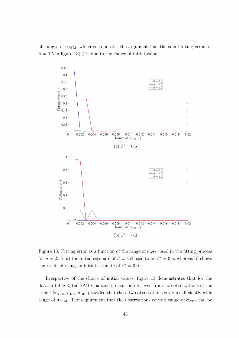
all ranges of σATM, which corroborates the argument that the small fitting error for

β = 0.5 in figure 13(a) is due to the choice of initial value.

0 0.002 0.004 0.006 0.008 0.01 0.012 0.014 0.016 0.018 0.02

Range of σATM (-)

0

0.05

0.1

0.15

0.2

0.25

0.3

0.35

0.4

0.45

Fittingerror(-)

β = 0.0β = 0.5β = 1.0

(a) β∗ = 0.5

0 0.002 0.004 0.006 0.008 0.01 0.012 0.014 0.016 0.018 0.02

Range of σATM (-)

0

0.2

0.4

0.6

0.8

1

Fittingerror(-)

β = 0.0β = 0.5β = 1.0

(b) β∗ = 0.0

Figure 13: Fitting error as a function of the range of σATM used in the fitting process

for n = 2. In a) the initial estimate of β was chosen to be β∗ = 0.5, whereas b) shows

the result of using an initial estimate of β∗ = 0.0.

Irrespective of the choice of initial values, figure 13 demonstrates that for the

data in table 8, the SABR parameters can be retrieved from two observations of the

triplet [σATM, σRR, σBF] provided that these two observations cover a sufficiently wide

range of σATM. The requirement that the observations cover a range of σATM can be

43

explained by remembering that each observation contains two constraints and that

we have three parameters to fit. Therefore we require at least two observations in

order to determine the parameter values uniquely. If the two observations cover a

very narrow range of σATM, then the constraints that they provide will be very similar

and we will, in effect, only have two constraints.

10.2 Effect of Noise on Fitting

In this section we investigate the stability of the fitting method described above in

the presence of noise. To simulate noisy market data, Gaussian noise was added to

the simulated market data as

σATM = σATM(1 + ε1)

σRR = σRR(1 + ε2)

σBF = σBF(1 + ε3), (82)

where each of the εi is drawn from an N(0,Σ2i ) distribution. The noise was chosen to

be proportional to the observed value to decrease the probability of obtaining negative

values for σATM or σBF.

10.2.1 Noisy σBF

First we investigate the effect of noisy σBF. That is we set Σ1 and Σ2 equal to zero

and vary Σ3. Repeating the methodology employed in section 10.1, we set n = 2

and investigate the influence of the range of σATM between the two observations.

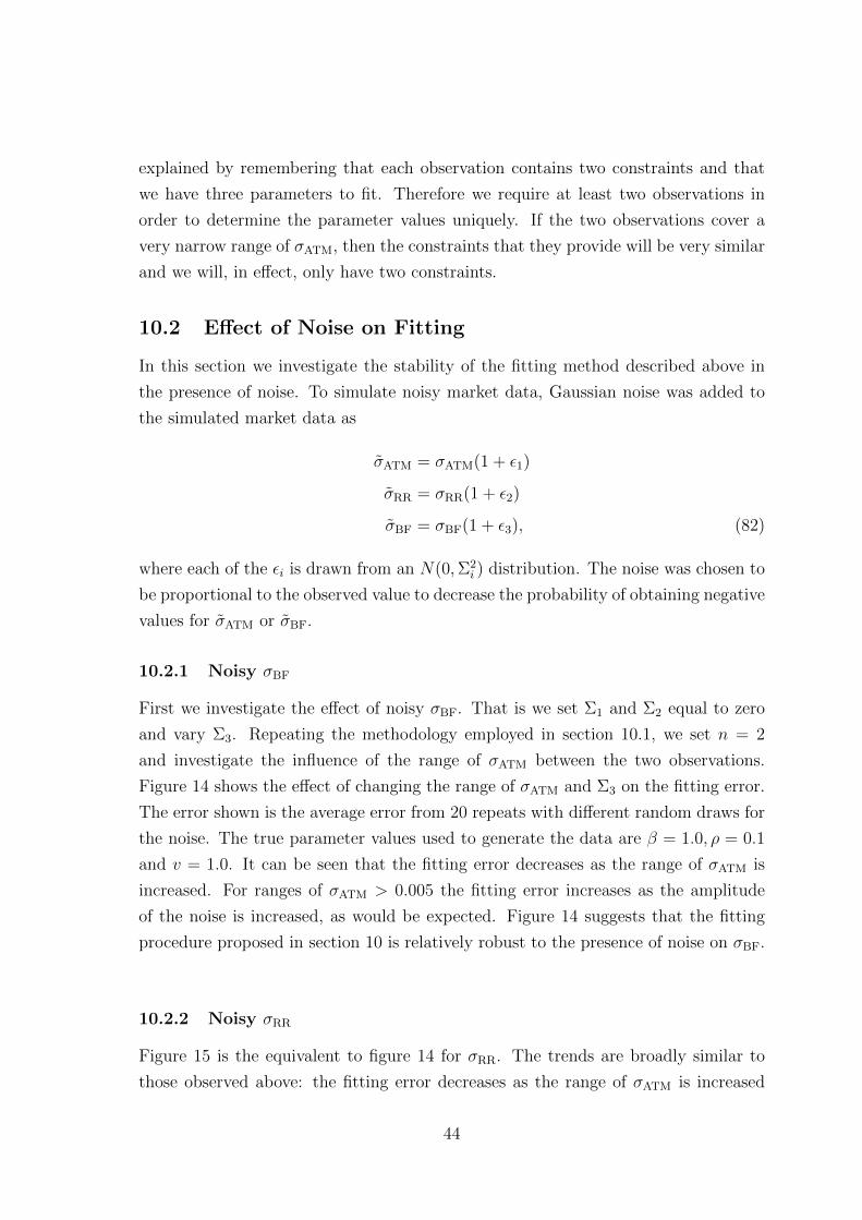
Figure 14 shows the effect of changing the range of σATM and Σ3 on the fitting error.

The error shown is the average error from 20 repeats with different random draws for

the noise. The true parameter values used to generate the data are β = 1.0, ρ = 0.1

and v = 1.0. It can be seen that the fitting error decreases as the range of σATM is

increased. For ranges of σATM > 0.005 the fitting error increases as the amplitude

of the noise is increased, as would be expected. Figure 14 suggests that the fitting

procedure proposed in section 10 is relatively robust to the presence of noise on σBF.

10.2.2 Noisy σRR

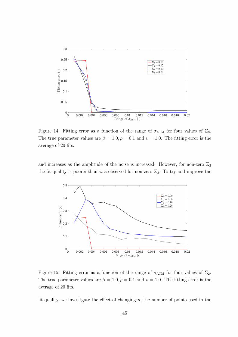
Figure 15 is the equivalent to figure 14 for σRR. The trends are broadly similar to

those observed above: the fitting error decreases as the range of σATM is increased

44

0 0.002 0.004 0.006 0.008 0.01 0.012 0.014 0.016 0.018 0.02

Range of σATM (-)

0

0.05

0.1

0.15

0.2

0.25

0.3

Fittingerror(-)

Σ3 = 0.00Σ3 = 0.05Σ3 = 0.10Σ3 = 0.20

Figure 14: Fitting error as a function of the range of σATM for four values of Σ3.

The true parameter values are β = 1.0, ρ = 0.1 and v = 1.0. The fitting error is the

average of 20 fits.

and increases as the amplitude of the noise is increased. However, for non-zero Σ2

the fit quality is poorer than was observed for non-zero Σ3. To try and improve the

0 0.002 0.004 0.006 0.008 0.01 0.012 0.014 0.016 0.018 0.02

Range of σATM (-)

0

0.1

0.2

0.3

0.4

0.5

Fittingerror(-)

Σ2 = 0.00Σ2 = 0.05Σ2 = 0.10Σ2 = 0.20

Figure 15: Fitting error as a function of the range of σATM for four values of Σ2.

The true parameter values are β = 1.0, ρ = 0.1 and v = 1.0. The fitting error is the

average of 20 fits.

fit quality, we investigate the effect of changing n, the number of points used in the

45

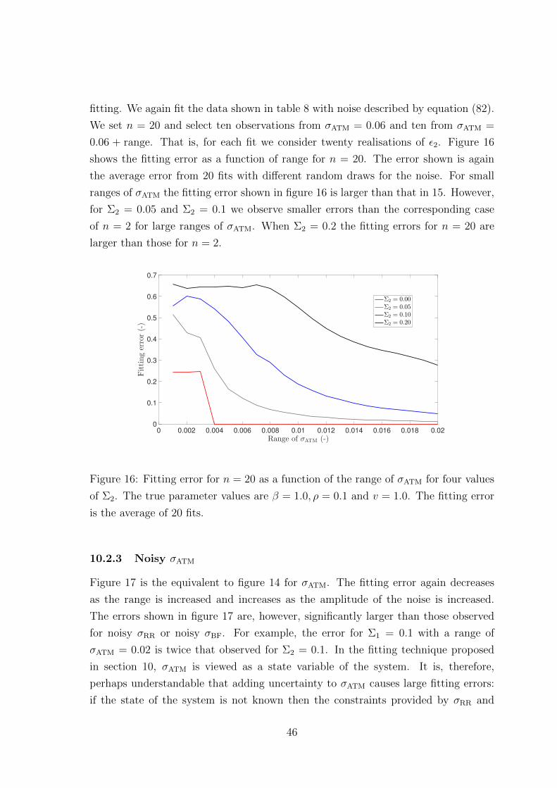
fitting. We again fit the data shown in table 8 with noise described by equation (82).

We set n = 20 and select ten observations from σATM = 0.06 and ten from σATM =

0.06 + range. That is, for each fit we consider twenty realisations of ε2. Figure 16

shows the fitting error as a function of range for n = 20. The error shown is again

the average error from 20 fits with different random draws for the noise. For small

ranges of σATM the fitting error shown in figure 16 is larger than that in 15. However,

for Σ2 = 0.05 and Σ2 = 0.1 we observe smaller errors than the corresponding case

of n = 2 for large ranges of σATM. When Σ2 = 0.2 the fitting errors for n = 20 are

larger than those for n = 2.

0 0.002 0.004 0.006 0.008 0.01 0.012 0.014 0.016 0.018 0.02

Range of σATM (-)

0

0.1

0.2

0.3

0.4

0.5

0.6

0.7

Fittingerror(-)

Σ2 = 0.00Σ2 = 0.05Σ2 = 0.10Σ2 = 0.20

Figure 16: Fitting error for n = 20 as a function of the range of σATM for four values

of Σ2. The true parameter values are β = 1.0, ρ = 0.1 and v = 1.0. The fitting error

is the average of 20 fits.

10.2.3 Noisy σATM

Figure 17 is the equivalent to figure 14 for σATM. The fitting error again decreases

as the range is increased and increases as the amplitude of the noise is increased.

The errors shown in figure 17 are, however, significantly larger than those observed

for noisy σRR or noisy σBF. For example, the error for Σ1 = 0.1 with a range of

σATM = 0.02 is twice that observed for Σ2 = 0.1. In the fitting technique proposed

in section 10, σATM is viewed as a state variable of the system. It is, therefore,

perhaps understandable that adding uncertainty to σATM causes large fitting errors:

if the state of the system is not known then the constraints provided by σRR and

46

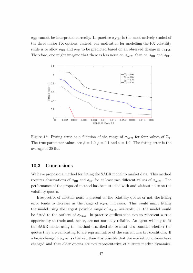
σBF cannot be interpreted correctly. In practice σATM is the most actively traded of

the three major FX options. Indeed, one motivation for modelling the FX volatility

smile is to allow σRR and σBF to be predicted based on an observed change in σATM.

Therefore, one might imagine that there is less noise on σATM than on σRR and σBF.

0 0.002 0.004 0.006 0.008 0.01 0.012 0.014 0.016 0.018 0.02

Range of σATM (-)

0

0.2

0.4

0.6

0.8

1

1.2

Fittingerror(-)

Σ1 = 0.00Σ1 = 0.05Σ1 = 0.10Σ1 = 0.20

Figure 17: Fitting error as a function of the range of σATM for four values of Σ1.

The true parameter values are β = 1.0, ρ = 0.1 and v = 1.0. The fitting error is the

average of 20 fits.

10.3 Conclusions

We have proposed a method for fitting the SABR model to market data. This method

requires observations of σRR and σBF for at least two different values of σATM. The

performance of the proposed method has been studied with and without noise on the

volatility quotes.

Irrespective of whether noise is present on the volatility quotes or not, the fitting

error tends to decrease as the range of σATM increases. This would imply fitting

the model using the largest possible range of σATM available, i.e. the model would

be fitted to the outliers of σATM. In practice outliers tend not to represent a true

opportunity to trade and, hence, are not normally reliable. An agent wishing to fit

the SABR model using the method described above must also consider whether the

quotes they are calibrating to are representative of the current market conditions. If

a large change in σATM is observed then it is possible that the market conditions have

changed and that older quotes are not representative of current market dynamics.

47

Therefore, we recommend choosing a large range of σATM subject to the caveats that

the quotes chosen are believed to represent genuine offers to trade; and that it is

believed that the market dynamics at the times the quotes were observed are relevant

to the current market conditions.

Assessing whether a fitting method is accurate enough to be useful is not straight

forward: factors to consider include how well the model describes the market and

how the model will be used. There is little value in accurately determining parameter

values if the model itself, irrespective of the choice of parameters, doesn’t capture

the features of the market that we are interested in. We should also consider the

impact of incorrect parameter estimation in terms of profit and loss: if we are using

a model in such a way that our profit and loss is very sensitive to a parameter value

then it is clearly important to determine the value of that parameter as accurately as

possible. Nevertheless, we are of the opinion that achieving a fitting error h ≤ 0.01 is

probably sufficient for most applications. This would, for example, be equivalent to

determining β to within ±0.1. In the absence of noise, the cases studied above met

this criterion when the range of σATM was greater than 0.005. We have also seen that

the model parameters can be accurately determined in the presence of noise on σBF.

Fitting in presence of noise on σRR or σATM is much more challenging and care would

be required if significant noise was observed on these quotes.

48

11 Example: Pricing a Digital Call

To demonstrate the importance of the correct determination of β, we consider a digital

call on a currency pair. The payoff of a domestic paying European digital call option

is

D(ST , K) =

1 if ST ≥ K

0 if ST < K.

The value of a domestic paying European digital call can be approximated as [13]:

D(S,K) = − ∂

∂KC(S,K, σ(K))

= −∂C(S,K, σ)

∂K− ∂C(S,K, σ)

∂σ

∂σ

∂K, (83)

where C(S,K, σ) is the price of a vanilla European call with strike K. The second

term is called the windmill-adjustment and is the product of the vega of a vanilla

option with strike K and the slope of the volatility smile at K.

Consider a situation where the evolution of the forward price, F , obeys the SABR

model with parameters β = 0.9, ρ = 0.2 and v = 1.0. The current ATM level is

σATM = 0.05 and we price a digital call option with strike ψ = ln(F/K) = −0.001

and time to expiry T−t = 0.5 using equation (83). For simplicity we assume that both

foreign and domestic interest rates are zero. The current forward price is F = 1.2.

The risk reversal and butterfly spread corresponding to these values are σRR = 0.517%

and σBF = 0.215%.

The price of the digital call is

D(S,K) = − ∂

∂KC(S,K, σ(K))

= Φ(d2)−K√T − tΦ′(d2)

∂σ

∂K, (84)

where

d2 =ψ − σ2

2(T − t)

σ√T − t

(85)

The implied volatility at ψ = −0.001 is given by equation (66) where q can be found

as the root of equation (67). For the data given above we find q = 0.04807 and

σ(−0.001) = 0.0501. We estimate the slope of the volatility smile at K using finite

differences:

∂σ

∂K≈σ(ln 1.2

1.2013)− σ(ln 1.2

1.2011)

0.0002

≈ 0.0901 (86)

49

Therefore the price of the digital call is

D(1.2, 1.2012) = 0.4817− 1.2012×√

0.5× 0.3985× (0.0901) (87)

= 0.4512 (88)

We now observe a step change in σATM from 0.05 to 0.1. Repeating the calculations

above for this new state yields a price of 0.4514.

11.1 Digital Pricing Assuming β = 0

Let us repeat the calculation above, this time assuming that we have chosen β = 0

based on prior knowledge. Fitting the market data σATM = 0.05, σRR = 0.517% and

σBF = 0.215% under the assumption that β = 0 yields the parameter values shown

in table 9. Table 10 compares the pricing of the digital option for the two values of

Table 9: SABR parameters for β = 0

β ρ v

0 0.2424 % 1.016 %

β. The two choices of β result in different values of D(F,K). At σATM = 0.05 the

difference between the two prices is negligible but at σATM = 0.1 we see that β = 0

results in a larger price than β = 0.9. Examining the data in table 10 reveals that

this difference is caused by different values for the slope of the volatility smile. The

two values of β result in the same values for σ(K). This is unsurprising since K is

very close to F and σ(F ) = σATM is used as a state variable to which both models

are fitted.

11.2 Accounting for σRR and σBF

In the above we priced a digital option at two different levels of σATM. For the

σATM = 0.1 level no use was made of σRR or σBF. This is possible because, for a

specified model, σATM is a state variable. That is, the volatility smile can be uniquely

determined if σATM, β, ρ and v are known. Above we considered the case of an agent

who observes a step change in σATM and uses this information to update their price

for a digital call. Let us now consider an agent who observes σRR and σBF in addition

to σATM.

50

Table 10: Digital option pricing

β = 0.9 β = 0.0 Refit

σATM 0.05 0.1 0.05 0.1 0.1

σ(K) 0.0501 0.1001 0.0501 0.1001 0.1001

d2 -0.0459 -0.0495 -0.0459 -0.0495 -0.0495

Φ(d2) 0.4817 0.4803 0.4817 0.4803 0.4803

Φ′(d2) 0.3985 0.3985 0.3985 0.3985 0.3985∂σ∂K

0.0901 0.0853 0.0913 0.0677 0.0877

D(F,K) 0.4512 0.4514 0.4508 0.4573 0.4506

The risk reversal and butterfly spread for β = 0.9, ρ = 0.2, v = 1.0 and σATM = 0.1

are σRR = 1.06% and σBF = 0.445%. For an agent who has determined the correct

SABR parameters, σRR and σBF provide no additional information and the price of

the digital call remains 0.4514. An agent who has selected β = 0.0 is able to refit their

model to the new market quotes and would obtain new parameter values as shown

in table 11. The pricing of the digital call option for these parameters is shown in

Table 11: Re-fitted SABR parameters for β = 0

β ρ v

0 0.2829 % 1.034 %

the final column of table 10. Using these parameter values the slope of the volatility

smile, and hence the digital call price, is much closer to those calculated with β = 0.9.

11.3 Discussion

In the above we examined the pricing of a digital option for different values of β. It

was observed that following a step change in σATM, different choices of β resulted in

different prices for the digital option and it was argued that the price difference arises

from differences in the slope of the volatility smile at K. We have also seen that

the price difference caused by a different choice of β can be significantly reduced by

re-fitting the model to updated values of σATM, σRR and σBF. This is in agreement

with the findings of other authors. For example, Hagan and Lesniewski [12] noted

that the SABR model can reproduce observed volatility smiles for any value of β.

51

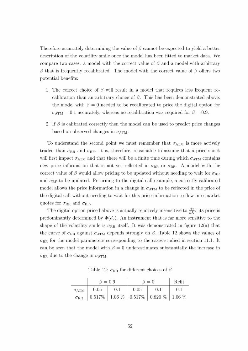
Therefore accurately determining the value of β cannot be expected to yield a better

description of the volatility smile once the model has been fitted to market data. We

compare two cases: a model with the correct value of β and a model with arbitrary

β that is frequently recalibrated. The model with the correct value of β offers two

potential benefits:

1. The correct choice of β will result in a model that requires less frequent re-

calibration than an arbitrary choice of β. This has been demonstrated above:

the model with β = 0 needed to be recalibrated to price the digital option for

σATM = 0.1 accurately, whereas no recalibration was required for β = 0.9.

2. If β is calibrated correctly then the model can be used to predict price changes

based on observed changes in σATM.

To understand the second point we must remember that σATM is more actively

traded than σRR and σBF. It is, therefore, reasonable to assume that a price shock

will first impact σATM and that there will be a finite time during which σATM contains

new price information that is not yet reflected in σRR or σBF. A model with the

correct value of β would allow pricing to be updated without needing to wait for σRR

and σBF to be updated. Returning to the digital call example, a correctly calibrated

model allows the price information in a change in σATM to be reflected in the price of

the digital call without needing to wait for this price information to flow into market

quotes for σRR and σBF.

The digital option priced above is actually relatively insensitive to ∂σ∂K

: its price is

predominantly determined by Φ(d2). An instrument that is far more sensitive to the

shape of the volatility smile is σRR itself. It was demonstrated in figure 12(a) that

the curve of σRR against σATM depends strongly on β. Table 12 shows the values of

σRR for the model parameters corresponding to the cases studied in section 11.1. It

can be seen that the model with β = 0 underestimates substantially the increase in

σRR due to the change in σATM.

Table 12: σRR for different choices of β

β = 0.9 β = 0 Refit

σATM 0.05 0.1 0.05 0.1 0.1

σRR 0.517% 1.06 % 0.517% 0.820 % 1.06 %

52

The two advantages of the fitting β discussed above are most beneficial during

large moves in σATM: small changes in σATM will not cause a large change in the

SABR parameters for any choice of β. Similarly, although ∂σRR

∂σATMdepends on β, small

changes in σATM can only cause small deviations in σRR, irrespective of the choice of

β.

However, as discussed in section 9, large changes in σATM are usually the result

of dramatic market events and it is doubtful whether the model parameters remain

constant during such events. With this is mind, it is not currently clear whether

accurately determining β offers any practical advantages compared to selecting an

arbitrary value of β and recalibrating the model on a regular basis.

53

12 Conclusions

Fitting the SABR model to market data is a challenging task because two of the model

parameters (β and ρ) both affect the skew of the volatility smile. It is frequently

claimed that β can be found from the slope of a log-log plot of historic values of σATM

against F . We have demonstrated here that this is not the case.

The SABR model is traditionally described as two correlated stochastic processes.

We have shown that, in an FX setting, the SABR model has a single state variable and

can be described by a single stochastic differential equation. When working with the

model it is useful to regard the at-the-money volatility, σATM, as the state variable of

the system because this can be observed directly in the market. The volatility smile is

then uniquely described by σATM and the three model parameters: β, ρ and v. Using

this representation we have shown how the model parameters can be retrieved from

observations of the volatility smile for two or more values of σATM.

Accurate determination of the SABR parameter values requires observations of

the volatility smile covering a sufficient range of σATM. For the parameter values

considered here a range of 0.005 was required to retrieve the parameter values from

simulated market data. We have presented three months of market data for EURUSD

and USDJPY. The range of σATM for both datasets was approximately 0.015, which

is larger than the minimum range required for the fitting method proposed here.

Fitting in the presence of noise has also been examined. Adding noise to σBF had

little effect on the ability to determine accurately the parameter values but larger

fitting errors were observed when noise was added to σATM or σRR.

12.1 Suggestions for Further Work

In this work we have considered methods for fitting the SABR model to FX data. We

have focused on simulated market data with known parameter values. An important

area for future work would be to examine how well the SABR model is able to describe

real market data. Specifically, we have seen that the SABR model predicts a unique,

deterministic relationship between σATM, σRR and σBF. At first glance this prediction

is not borne out by the market data shown in figures 8 and 11. Future work could

examine the source of this discrepancy. Do the SABR parameters change over time

such that the model predictions hold over shorter timeframes or is there a pattern to

discrepancies between the market observations and the model predictions?

One motivation for modelling the FX market using the SABR model is that it

establishes a relationship between σATM, σRR and σBF. In section 11.3 we considered

54

that new price information might affect σATM before it is reflected in σRR and σBF. An

important aspect of further work would be to establish whether this idea is supported

by historical data. Therefore we would propose using signal analysis techniques to

establish whether there is evidence of a time lag between σRR, σBF and σATM. It

would be interesting to know whether the magnitude of any such lag is constant or

whether it depends on market conditions.

Finally we would recommend an examination of historic market data from events

which caused step-changes in the FX market, for example the UK referendum on EU

membership on 26 July 2016 or the removal of the ‘peg’ in the EURCHF market on

15 January 2015. Analysis of these events, which sent shock waves through the FX

markets, could focus on two key questions in regard to this work:

1. If we model the market using the SABR model, is there any evidence that model

parameters are preserved during dramatic events?

2. Is there evidence of a time lag between σATM, σRR and σBF during such events?

Answering these questions would help to determine whether the correct determination

of β offers useful advantages over using an arbitrary value of β and re-fitting the model

on a frequent basis.

55

References

[1] P. S. Hagan, D. Kumar, A. S. Lesniewski, and D. E. Woodward. Managing smile

risk. Wilmott, 1:84–108, 2002.

[2] A. Castagna. FX Options and Smile Risk. John Wiley and Sons Ltd, 2010.

[3] D. Reiswich. An empirical comparative analysis of foreign exchange smile cali-

bration procedures. J. Comput. Financ, 60:31–67, 2011.

[4] Jan Obloj. Fine-tune your smile : Correction to Hagan.

http://arxiv.org/abs/0708.0998, 2008.

[5] H. Berestycki, J. Busca, and I. Florent. Hedging under SABR model. Comm.

Pure Appl. Math., 57:1352–1373, 2004.

[6] G. West. Calibration of the SABR model in illiquid markets. Appl. Math.

Finance, 12:371–385, 2005.

[7] P. Nowak and P. Sibetz. Volatility smile.

http://www.fam.tuwien.ac.at/∼sgerhold/pub files/sem12/s sibetz nowak.pdf,

2012.

[8] F. Le Floc’h and G. Kennedy. Explicit SABR calibration through simple explan-

sions. SSRN eLibrary, 2014.

[9] P. S. Hagan, D. Kumar, A. S. Lesniewski, and D. E. Woodward. Arbitrage free

SABR. Wilmott, 69:60–75, 2014.

[10] S. Skov Hansen. The SABR model - theory and application. PhD thesis, Copen-

hagen Business School, 2011.

[11] B. Bartlett. Hedging under SABR model. Wilmott, July/August:68–70, 2006.

[12] P. S. Hagan and A. S. Lesniewski. Bartlett’s delta in the SABR model.

http://dx.doi.org/10.2139/ssrn.2950749, 2017.

[13] U. Wystrup. FX Options and Structured Products. John Wiley and Sons Ltd,

2017.

56

Appendices

A Python Code

Listing 1: The SABR class. Used to calculate σRR and σBF for specified model

parameters and values of σATM

class SABR:def i n i t ( s e l f , a rgs ) :

s e l f . beta = args [ 0 ]s e l f . rho = args [ 1 ]s e l f . vo l = args [ 2 ]s e l f . atm = args [ 3 ]s e l f . v r r = args [ 4 ]s e l f . v b f = args [ 5 ]s e l f . t ex = args [ 6 ]

def ca lc atm ( s e l f , a rgs ) :q = args [ 0 ]term1 = s e l f . t ex ∗( q∗∗2∗(1.0− s e l f . beta )∗∗2/24 .0 + \

0 .25∗ s e l f . rho∗ s e l f . beta ∗ s e l f . vo l ∗q + \s e l f . vo l ∗∗2/24.0∗(2 .0−3.0∗ s e l f . rho ∗∗2))

atm = q∗(1.0+ term1 )return atm

def atm error ( s e l f , a rgs ) :return s e l f . atm − s e l f . ca lc atm ( args )

def s e t q ( s e l f ) :s o l = root ( s e l f . atm error , s e l f . atm)s e l f . q = s o l . x

def volAtDelta ( s e l f , a rgs ) :s e l f . d e l t a = argss o l = root ( s e l f . c a l c v o l d i f , s e l f . atm)return s o l . x

def c a l c v o l d i f ( s e l f , a rgs ) :#Ca l cu l a t e s the d i f f e r e n c e between a t a r g e t v o l and the#vo l a t d e l t avo l = args [ 0 ]d e l t a = s e l f . d e l t aw = np . s i gn ( s e l f . d e l t a )q = s e l f . qp s i = w∗ vo l ∗ s q r t ( s e l f . t ex )∗Ninv (abs ( d e l t a ) ) \− 0 .5∗ vo l ∗∗2∗ s e l f . t ex

i f p s i ==0.0:I0 = q

else :i f s e l f . beta==1:

z = s e l f . vo l /q ∗ p s ielse :

z = s e l f . vo l /q ∗ (1.0− exp(−p s i ∗(1.0− s e l f . beta ) ) )\/(1.0− s e l f . beta )

ch i = log ( ( s q r t (1.0−2.0∗ z∗ s e l f . rho+z∗∗2)+z−s e l f . rho )\/(1− s e l f . rho ) )

I0 = s e l f . vo l ∗ p s i / ch i

term1 = s e l f . t ex ∗( q∗∗2∗(1.0− s e l f . beta )∗∗2/24 .0\

57

∗exp ( p s i ∗(1.0− s e l f . beta ) ) + \0 .25∗ s e l f . rho∗ s e l f . beta ∗ s e l f . vo l ∗q\∗exp ( p s i ∗(1.0− s e l f . beta ) / 2 . 0 ) + \s e l f . vo l ∗∗2/24.0∗(2 .0−3.0∗ s e l f . rho ∗∗2))

return I0 ∗(1.0+ term1)−vo l

def c a l c s t r i k e s ( s e l f ) :#Ca l cu l a t e s the v o l a t i l i t i e s a t d e l t a s o f 0.25 and −0.25s e l f . c a l l = s e l f . volAtDelta ( 0 . 2 5 )s e l f . put = s e l f . volAtDelta (−0.25)

def c a l c r r ( s e l f ) :return s e l f . c a l l − s e l f . put

def c a l c b f ( s e l f ) :return 0 . 5∗ ( s e l f . c a l l + s e l f . put ) − s e l f . atm

Listing 2: The q data class. For a specified SABR model it creates lists of σRR and

σBF for σATM between 0.06 and 0.08.class q data :

def i n i t ( s e l f , a rgs ) :s e l f . beta = args [ 0 ]s e l f . rho = args [ 1 ]s e l f . vo l = args [ 2 ]s e l f . t ex = args [ 3 ]s e l f . atm = np . l i n s p a c e ( 0 . 0 6 , 0 . 08 , num=21)s e l f . v r r = [ ]s e l f . v b f = [ ]s e l f . q = [ ]#Get q from atmfor i in s e l f . atm :

x = [ s e l f . beta , s e l f . rho , s e l f . vol , i , i , i , s e l f . t ex ]smi l e = SABR( x )smi l e . s e t q ( )s e l f . q . append ( smi l e . q )smi l e . c a l c s t r i k e s ( )s e l f . v r r . append ( smi l e . c a l c r r ( ) )s e l f . v b f . append ( smi l e . c a l c b f ( ) )

Listing 3: Function to be minimised. Implements equation (80).

def e r r o r q ( args , po ints , step , s ta r t , r epea t s ) :beta = args [ 0 ]rho = args [ 1 ]vo l = args [ 2 ]e r r = 0 .0np . random . seed ( seed= 2000)

for j in range ( s t a r t ) :no i s e = Ninv (np . random . rand ( ) )

for i in range ( po in t s ) :for p in range ( r epea t s ) :

no i s e = Ninv (np . random . rand ( ) )key = i ∗ s tepatm = qd . atm [ key ]v b f = qd . v b f [ key ]v r r = qd . v r r [ key ] ∗(1.0+ no i s e ∗0 . 05 )

58

x = [ beta , rho , vol , atm , v bf , v r r , t ex ]SABRsmile [ key ] = SABR( x )SABRsmile [ key ] . s e t q ( )SABRsmile [ key ] . c a l c s t r i k e s ( )e r r += ( SABRsmile [ key ] . c a l c b f ( )/ v bf −1.0)∗∗2e r r += ( SABRsmile [ key ] . c a l c r r ( )/ v rr −1.0)∗∗2

return e r r

Listing 4: The main program minimises error q using the L-BFGS-B method. We

loop over the step size between the points to be fitted. At each step size repeats

repeats are performed and the result is the average error over these repeats.#Bounds on beta , rho and vbnds = ( ( 0 . 0 , 1 . 0 ) , ( − 0 . 9 , 0 . 9 ) , ( 0 . 0 , 1 0 0 . 0 ) )

#I n i t i a l guess f o r beta , rho , vx0 = np . array ( [ 0 . 5 , 0 . 0 , 0 . 5 ] )#True va l u e s o f beta , rho , vx = np . array ( [ 1 . 0 , 0 . 1 , 1 . 0 ] )

writeArray = [ ]maxPoint = 20 #Max number o f s t e p s between the 2 po in t s used in the f i t t i n gr epea t s = 20 #Number o f f i t s performed f o r averag ingrp t s = 1 #Number o f po in t s at each va lue o f ATM

#Create the smi l e data to be f i t t e d .qd = q data ( [ x [ 0 ] , x [ 1 ] , x [ 2 ] , t ex ] )

#Use 2 po in t sfor i in range ( maxPoint ) :

e r r = np . array ( [ 0 . 0 , 0 . 0 , 0 . 0 ] )for j in range ( r epea t s ) :

r e s = minimize ( e r ro r q , x0 , \args = (2 , i +1 ,2∗ j ∗ rpts , rp t s ) , \method=’L−BFGS−B ’ , bounds=bnds , \opt ions={ ’ d i sp ’ : Fa l se })

e r r += [ ( r e s . x [0]−x [ 0 ] ) ∗ ∗ 2 , \( r e s . x [ 1 ] / x [1]−1)∗∗2 , ( r e s . x [ 2 ] / x [2]−1)∗∗2 ]

e r r = e r r / r epea t swriteArray . append ( [ ( i +1)∗0.01 , e r r [ 0 ] , e r r [ 1 ] , e r r [ 2 ] ] )

59