calculating return on investment of training using process ... · calculating return on investment...
TRANSCRIPT

Calculating Return on Investment of Training using process
variation
Journal: IET Software
Manuscript ID: SEN-2011-0024.R1
Manuscript Type: Research Paper
Date Submitted by the Author:
n/a
Complete List of Authors: Matalonga, Santiago; Universidad ORT Uruguay, Facultad de Ingeniería San Feliu, Tomás; Universidad Politécnica de Madrid, Facultad de Infomrática
Keyword: STATISTICAL PROCESS CONTROL, SOFTWARE ENGINEERING, SOFTWARE METRICS
IET Review Copy Only
IET Software
1
Calculating Return on Investment of Training using
process variation
Santiago Matalonga1, Tomás San Feliu.
2
1Cuareim 1141, 11100. Montevideo, Uruguay. Facultad de Ingeniería. Universidad ORT Uruguay.
2Campus de Montegancedo. Boadilla del Monte, España. Facultad de Informática. Universidad Politécnica
de Madrid.
[email protected], [email protected]
Abstract
Organizations have relied on training to increase the performance of their workforce. Also, software
process improvement models suggest that training is an effective tool for institutionalizing a development
process. Training evaluation becomes important for understanding the improvements resulting from the
investments in training.
Like other production process, the software development process is subject to natural and special
causes of variation, and process improvement models recommend its statistical management.
Return on investment (ROI) has already been proposed as an effective measure to evaluate training
interventions. Nevertheless, when applying ROI in production environments, practitioners have not taken
into consideration the effects of variation in production processes.
This paper presents a method for calculating ROI that considers process variation; we argue that ROI
results should be understood in accordance to statistical management guidance.
The proposed method has been piloted at a software factory. The results of the case study are reported.
These results show how to calculate ROI by taking into account the variation of a production process.
Keywords: Statistical Process Control, Return on Investment, Training, Software Engineering
1 Introduction
Process improvement models like CMMI[1], ISO[2, 3] or Six sigma [4] have grown in popularity and
adoption in the recent years [5]. One aspect that these models have in common is that they rely on training as a
Page 1 of 20
IET Review Copy Only
IET Software

2
method to change the behavior of the workforce. For instance CMMI has a process area devoted to
organizational training; likewise the ISO family has clauses which are specifically aimed at delivering the
necessary training for the people executing the processes.
It has been reported that organizations invest an annual average of 100 million US dollars in training [6],
such amounts require that organizations find reliable ways to evaluate the return on their investment in training.
Methods of return on investment (ROI) have been proposed as a solution for this problem[7, 8]. We
nevertheless believe that ROI mechanisms have some limitations that practitioners must take into account.
First, ROI results are often given in absolute numbers (for instance [9] calculates a direct ROI of 200% for a
process improvement initiative). We believe that these methods do not satisfactory address the reality that all
production environments exhibit variation [10]. We argue that decision based on average figures can lead
management into wrong conclusion. While with statistical management, managers have visibility into the risks
and opportunities associated with variation [11].
Second, there is no clear consensus about when the ROI calculation must be carried out. The knowledge or
skill taught at the training intervention must be given time to be assimilated [12]. Also, the opportunities on the
job must appear for the individual to apply the received knowledge or skill [13]. It is beyond the scope of this
proposal to determine which the best control point to perform ROI calculation is. This is a subject of research
among training evaluation researchers [12, 14]. Nevertheless, we will argue that the automation of this proposal
is simple and therefore can help organizations mitigate this problem.
This paper proposes a method to calculate ROI that considers the natural variation of the production process.
The objective of this method is to provide training managers with quantitative information which can be used to
make reliable decisions about the effectiveness of a training intervention. The method presented in this paper
has been piloted at a software development organization and quantitative results of the case study are also
presented in this paper. Furthermore, we present a discussion of the validity of the results of the case study.
This paper is organised as follows:
Section 2 provides an overview of the current state of the art of ROI as it applies to training interventions.
Section 3 provides an overview of statistical process control. The focus of this section is to establish what
process control graphs are and how to construct them.
Section 4 details the process for calculating ROI that accounts for the variation of the production process.
Section 5 presents the results of the case study conducted in a software development factory.
Page 2 of 20
IET Review Copy Only
IET Software

3
Section 6 presents a discussion of the obtained results and an analysis of the uncontrolled variables in the
pilot study.
Section 7 analyzes the threats to validity of the obtained results.
Finally, we present our conclusions and discuss further lines of research.
2 Training evaluation and ROI on training
The literature on training evaluation is dominated by Kirkpatrick’s model [15, 16, 17]. The model defines
four levels at which an organization should be interested in obtaining measures about a training intervention:
• Reaction: Measures how participants felt during the training activity. Evaluating reaction is usually
simple, cost-effective, and accomplished by asking trainees to complete surveys.
• Learning: Measures the improvement of a trainee at a certain skill or knowledge because of the training
intervention. Learning measures are usually obtained by applying pre and post tests during a training
event.
• Behaviour or Transfer: Measures how much of the acquired knowledge was successfully applied on the
job. Transfer measures, are the first level of measures that the organization should have interest in
because they show how the effort invested in training has a return in the job.
• Results: This level is about bottom-line results. It implies collecting data about the degree in which
training was able to influence the organization objectives.
Kirkpatrick model has been the dominant model in training literature until the early 1990’s when other
researchers evolving it by looking into successful application of it in the industry [6, 13, 18]. Researchers have
not been successful at predicting results of higher levels from measures in lower levels [13, 18, 19]. Which have
lead other authors to question the foundations of the model by classifying it as taxonomy [6, 20, 21]. They argue
that a model should allow the practitioners to make inferences.
Nevertheless, according to [22, 23, 24] the greatest strength of the Kirkpatrick’s model is its simplicity.
Notwithstanding, this simplicity also led to a gap between the state of the art and the state of the practice[17],
which has been attributed to a lack of practical guidance on how to achieve measurement on each of the four
levels.
The application of ROI to training interventions was proposed by Phillips [7] as a fifth level. Phillips main
enhances Kirkpatrick’s model with systematic guidance to help organizations evaluate training in terms of
Return on Investment. To calculate ROI, Phillips applies the following ROI formula:
Page 3 of 20
IET Review Copy Only
IET Software

4
(1) ( )
*100Benefits Costs
ROICosts
−=
Most critics of Phillips approach lie on an excessive emphasis on monetary data when measuring
interventions whose aims are to develop intangible soft skills [20, 25, 26]. In addition to this, it has been noted
that the ROI formula does not considers the time factor [27, 28]. This is the period since the investment, or
intervention, until the moment the organisation collects the benefits. ROI results must be accompanied by a time
reference in order to allow comparison with other types of investment.
In the software industry ROI has also been used to account for the investment in training [29, 30, 31, 32]. For
instance, ROI is used to justify the investment in SEI´s Team Software Process [33] training.
With ROI calculations, it is usually the case that cost factors are know and that the organizations accounting
system is already tracking them. In contrast, benefits are harder to identify and usually there needs to be
agreement among stakeholders involved in analyzing the results. In training interventions, increased benefits
should come in the form of increased performance of the workforce. When applying Equation (1), benefits will
be calculated by estimating/measuring the difference between benefits before and after the training intervention.
Most often, some sort of proxy variable like production defects (for instance see [33]) is used to measure this
difference. Our approach is based on the application of statistical process control to the question of measuring
the variation before and after the intervention.
3 Statistical Process Control
Statistical process control (SPC) is an economical way of managing and controlling a process output. Since
the quality of a product is highly influenced by the quality of the process used to manufacture it [34, 35]. It is
reasonable to control the process in order to control the products’ quality.
SPC was pioneered by the work of Shewhart. In his work [35], he laid the foundation for several of the SPC
techniques currently used.
SPC has been widely accepted in the manufacturing industry [11]. Nevertheless, SPC has had a relatively low
penetration in the software industry. According to a study conducted by the SEI [36], high maturity
organisations only account for 10% of the published appraisal results. Furthermore, a recently released survey
shows that most high maturity organizations are not applying the SPC concepts correctly in their processes[37].
From the available SPC techniques, in this paper we have applied process control charts, which are explained
in the following section.
Page 4 of 20
IET Review Copy Only
IET Software

5
3.1 Process control charts
All processes exhibit variation, but whereas some of the variation can be expected from the construction of
the process (“natural cause of variation”), other variations can be assigned to special causes of variation [38].
Special causes of variation can be analysed and root causes identified; thus process improvement can be put in
place to prevent them from happening again.
Process control charts (PCCs) provide the ability to differentiate between natural and special causes of
variation. With PCC it can be determined if a process is “in control” or not. When a process is in control, past
performance can reasonable be extrapolated to predict future performance [39]. This is a characteristic of stable
process that we will take into consideration when making decisions about the repeatability of a training
intervention.
PCCs can be constructed with relatively few data points. At least three points are needed to construct a
control chart. As the dataset grows, the control chart becomes more descriptive in its ability to identify special
from natural causes of variation.
Run charts are the types of PCC identified as most feasible to construct [10] (hence, the ones we will use
throughout this study). The key to constructing run charts is identifying the upper and lower control limits that
distinguishes special causes of variation from natural causes of variation [34, 38].
Traditionally, control limits were established at three standard deviations from the mean [10]. Wheeler’s
approach involves plotting the process output and the process-by-process variation, called the moving range
chart. Analyzing the moving range chart and the run chart together, gives better visual indications of which
processes are in control.
With the presentation of both run charts side by side, special causes of variation can be observed in the
graphs by following a reduced set of heuristics [38] (when compared with the traditional approach). When using
both run charts, a process is defined as being in control if none of the following conditions is met:
• Test 1: A single point falls outside the control limit.
• Test 2: At least two of three successive values fall on the same side of, and more than two sigma units
away from, the centre line.
• Test 3: At least four out of five successive values fall on the same side of, and more than one sigma
unit away from, the centre line.
• Test 4: At least eight successive values fall on the same side of the centre line.
The process control lines are calculated as follows [38]:
Page 5 of 20
IET Review Copy Only
IET Software

6
• The central line is the average of the process output values ( X ).
• The upper control limit (UCL) is calculated with the following equation:
*UpperControlLimit X a mR= +
• The lower control limit (LCL) is calculated with the following equation:
*LowerControlLimit X a mR= −
Where mR is called the moving range, as it defined as the difference in absolute value of two consecutive
process output values.
1i imR x x−
= −
mR stands for the average of the moving range values. As it is shown in [38], for n individual process output
values there are n-1 moving range values. The equation for the average moving range is:
1
2
1
n
i ix x
mRn
−−
=−
∑
The upper range limit is calculated with the following equation:
*UpperRangeLimit b mR=
Factor a and b, are tabulated depending on process output that is being studied. A discussion and decision
tree for their values for software engineering variables can be found in [39] and is summarized in Table 1.
Variable Data Attribute Data
Data characterized by
Binomial Model
Data characterized by Poisson
Model
Other data based
on counts
Group
Series
Individual
output
N constant N variable Constant Variable Constant Variable
X- Bar
Range
Chart
Individual
&
Moving
Range
Np chart
XmR
p chart or
XmR
p chart or XmR p chart or
XmR
XmR
charts
for
counts
XmR
chart
for
Ranges
Table 1 Types of run charts
Page 6 of 20
IET Review Copy Only
IET Software

7
In the case study of this paper, defects will be used as a proxy for improved training; this means that a
discrete data will be used to represent a continuous variable. Given the previous discussion, the parameter
values for individual output of non grouped data are: a=2.66 and b = 3.27 [39].
4 Applying Statistical Process Control to Return on
Investment
This section presents a method for calculating Return on Investment that it takes into consideration the
natural variation of the production process.
When measuring performance in a production environment we suggest that practitioners should consider the
natural variation of the productive activities. This will enable them to see the actual range of the return of their
investment instead of a number that is based on averages.
Since production is subject to natural variation, a value by average approach can lead to incorrect
conclusions. In order to assert that improvement has occurred, control limits must shift in the direction of the
business goal. Without SPC there can be no statistical assurance of actual improvement having occurred.
Therefore, we propose that training should be evaluated in accordance with the observed change in process
performance. This is, by studying the shifts of the control limits of the process.
We believe that the following two considerations must be taken into account when calculating ROI in
production environments (which in our case is represented by the software development process):
• Natural process variation. When estimating benefits, the classical ROI formula does not take process
variation into consideration.
• Accommodation for the time factor. All ROI results will be accompanied by a time factor so that the
results can be compared to other investments [27, 28].
4.1 A method for calculating ROI of training interventions that considers process variation
The aforementioned difficulty in establishing benefits parameters requires that the proposed method provides
some preconditions for it to be applied in a software organization. These preconditions are presented in Step 0.
They mainly aim at setting conditions for the organization´s measurement infrastructure.
In addition to this, this process will not determine when the calculation must be carried out. As it was
mentioned, ROI results for training interventions can have significant changes depending on the moment the
Page 7 of 20
IET Review Copy Only
IET Software
8
calculation is conducted. Evaluating the intervention too early might not give time for the subjects to assimilate
the acquired knowledge [12, 40, 41]. The implementing organization must decide which the best moment to
conduct the evaluation is.
Nevertheless, we advocate that should be cost effective to embed the calculation within the organization’s
measurement system (in [42] we present how this automation was achieved in the organization under study).
Automation will allow the practitioners to evaluate ROI at different points in time.
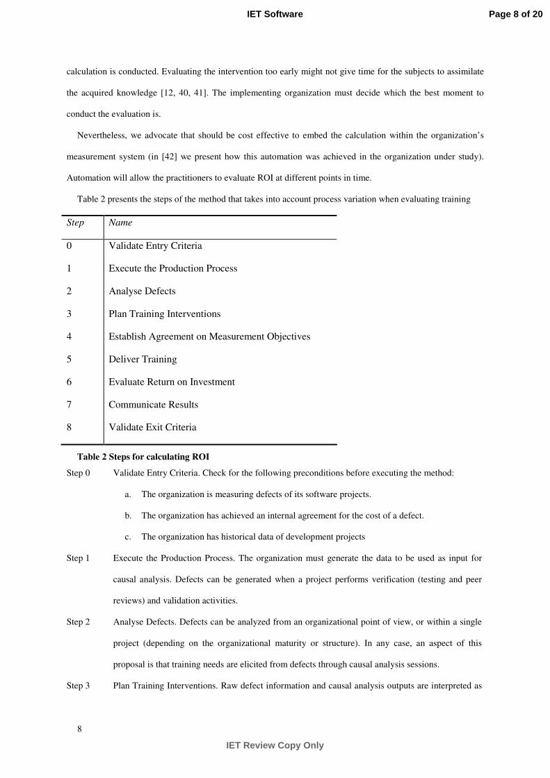
Table 2 presents the steps of the method that takes into account process variation when evaluating training
Step Name
0 Validate Entry Criteria
1 Execute the Production Process
2 Analyse Defects
3 Plan Training Interventions
4 Establish Agreement on Measurement Objectives
5 Deliver Training
6 Evaluate Return on Investment
7 Communicate Results
8 Validate Exit Criteria
Table 2 Steps for calculating ROI
Step 0 Validate Entry Criteria. Check for the following preconditions before executing the method:
a. The organization is measuring defects of its software projects.
b. The organization has achieved an internal agreement for the cost of a defect.
c. The organization has historical data of development projects
Step 1 Execute the Production Process. The organization must generate the data to be used as input for
causal analysis. Defects can be generated when a project performs verification (testing and peer
reviews) and validation activities.
Step 2 Analyse Defects. Defects can be analyzed from an organizational point of view, or within a single
project (depending on the organizational maturity or structure). In any case, an aspect of this
proposal is that training needs are elicited from defects through causal analysis sessions.
Step 3 Plan Training Interventions. Raw defect information and causal analysis outputs are interpreted as
Page 8 of 20
IET Review Copy Only
IET Software

9
the training needs of the project.
Step 5 Establish Agreement on Measurement Objectives: Stakeholders must obtain agreement on how the
training results will be measured. This probably will depend on decisions made in the previous two
steps. It is recommended that senior management is involved during the selection or validation of
the variable used to measure training effectiveness agreement. Techniques like Goal-Question-
Metric[43], QFD[44], GOSPA [44] or reality trees [45] can be used to achieve this.
Step 5 Deliver Training. Training must be delivered according to the organisation’s standard training
process.
Step 6 Evaluate ROI. In order to calculate ROI for the training interventions, the cost and benefits of the
interventions must be identified:
a. Costs: Costs included for this proposal can be training costs (including preparation and
delivery); and defects analysis costs.
b. Benefits: This is the key aspect of the method and it is explained in section 4.2.
Step 7 Communicate Results. The execution of the method should enable the training department to
communicate the results of the training interventions in terms of ROI.
Step 8 Validate Exit Criteria. After execution of this process, the organisation should have:
a. Performed causal analysis and reported the results.
b. The training department has planned and executed training interventions
c. The results of the training interventions have been communicated in terms of ROI.
4.2 Evaluate ROI
As with any ROI calculation, costs parameters are easier to identify than the benefits parameters. In this case
we propose to take into account the costs of performing a causal analysis of defects, and the cost of delivering
the training. Causal analysis of the projects’ defects is used as input to select the necessary training to be
delivered (step 3). Training costs includes the costs of preparing and delivering the training (in [46, 47] a
discussion of the cost factors that can be taken into account is presented).
We propose to calculate benefits in terms of defect reduction. This is the same assumption that is used in the
Team Software Process [33]. Benefits will be calculated by comparing the defect count before and after the
training intervention. To compute the benefits, the average cost of a defect will be used.
HistoricMeanBenefits Defects CostOfADefect= ∆ ×
Page 9 of 20
IET Review Copy Only
IET Software

10
In order to calculateDefects∆
, we propose to apply SPC to the defect calculation. Figure 1 shows how this
is carried out. A defect baseline must be established. The observed variation of the control limits before and
after the training intervention will be used to calculate the benefits and provide the range of return on investment
for the training intervention.
Figure 1 Method for calculating ROI
1. Determine Historical Sample.
The organisation must determine the projects from the historical database that will be included in the sample.
Selection criteria should be in line with the scope of the training to be imparted (usually type of project, size, or
technology). After the projects have been selected, the organisation must apply the statistical techniques
reviewed in section 3 in order to establish the performance baseline. UCL and LCL of the historical sample
determine the performance baseline.
2. Deploy and execute the process.
The organisation must determine the project or projects in which the training intervention will be deployed.
3. Evaluate Data Availability.
As seen in section 3, at least three data points are needed in order to calculate new control limits for the
projects that have applied the process.
4. Estimate ROI.
Page 10 of 20
IET Review Copy Only
IET Software
11
As a general rule, when there is not sufficient data available to establish new control limits, ROI calculation
will be performed according to the following rule:
• Worst Case: upper control limit of the historic sample, compared to observed defects in the project.
• Real Case: historic mean compared to observed defects in the project.
• Best Case: lower control limit compared to observed defects in the project.
5. Establish actual control limits.
Actual control limits are obtained by applying the techniques reviewed in section 3 to the data from the
projects that have received training.
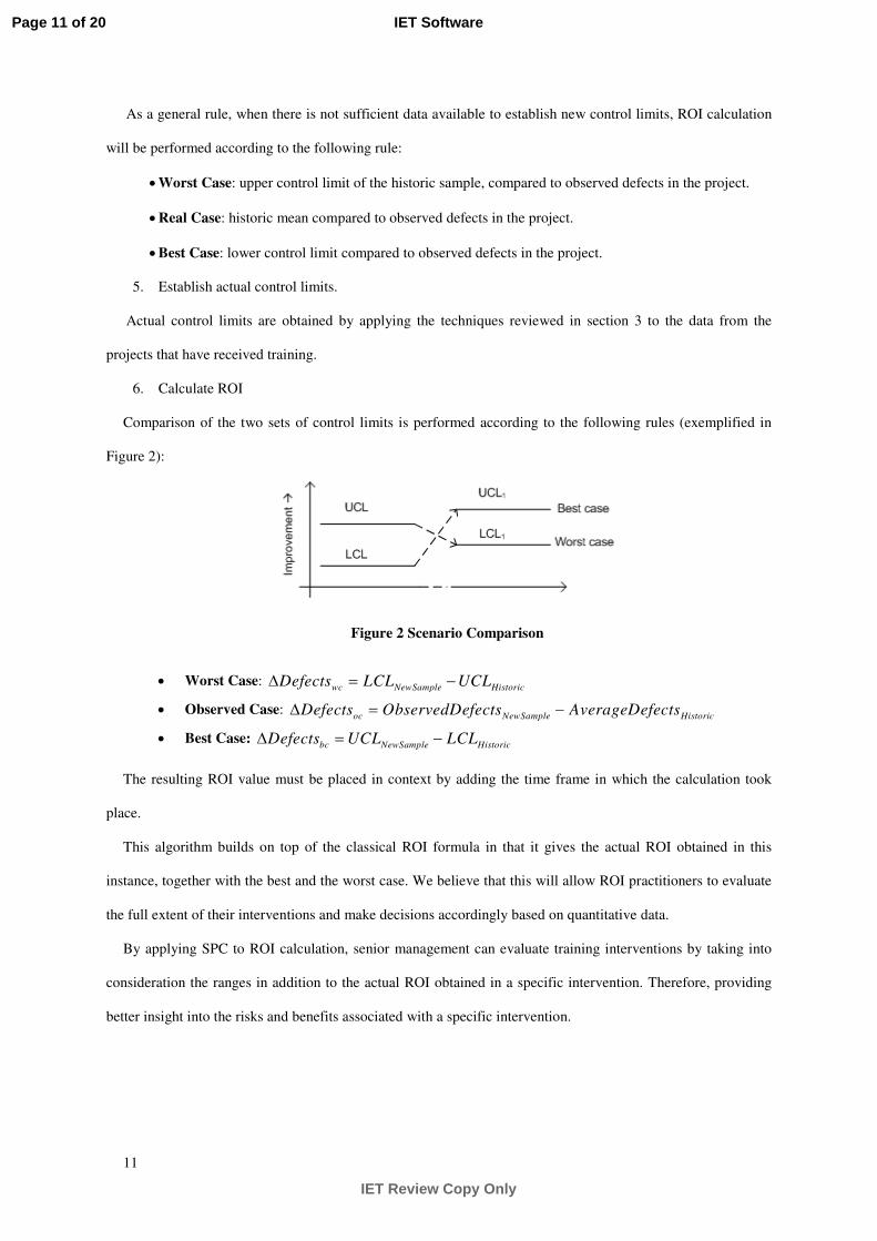
6. Calculate ROI
Comparison of the two sets of control limits is performed according to the following rules (exemplified in
Figure 2):
Figure 2 Scenario Comparison
• Worst Case: wc NewSample HistoricDefects LCL UCL∆ = −
• Observed Case: oc NewSample HistoricDefects ObservedDefects AverageDefects∆ = −
• Best Case: bc NewSample HistoricDefects UCL LCL∆ = −
The resulting ROI value must be placed in context by adding the time frame in which the calculation took
place.
This algorithm builds on top of the classical ROI formula in that it gives the actual ROI obtained in this
instance, together with the best and the worst case. We believe that this will allow ROI practitioners to evaluate
the full extent of their interventions and make decisions accordingly based on quantitative data.
By applying SPC to ROI calculation, senior management can evaluate training interventions by taking into
consideration the ranges in addition to the actual ROI obtained in a specific intervention. Therefore, providing
better insight into the risks and benefits associated with a specific intervention.
Page 11 of 20
IET Review Copy Only
IET Software
12
5 Experimentation
The results presented in this section were obtained while we were working with a software factory located in
Montevideo, Uruguay. This software factory has been operating since the year 2000, and it was rated at CMMI
Maturity Level 3 in 2007.
It is important to note that statistical control is not required at CMMI Maturity Level 3, and that this
organization had not implemented statistical control for its processes. The run charts presented in this case study
were created by the researchers and are not being used by the organization in its every day practice.
5.1 Tailoring the method for the organization under study
The concept of process tailoring implies that a project should be able to adapt an organizational standard
process so that the resulting tailored process can better suit the process needs[1]. This section describes how the
proposed method was tailored to the environment of the organization under study.
The case study was carried out between the years 2007 and 2008. The organization selected in which of the
three product lines to deploy the method.
The selection of the training intervention (Step 2) was carried out by the organizations’ resources following a
causal analysis process supervised by the researchers [42, 46]. Training was aimed at improving resources skills
in managing requirements and in operating the change management tool (Step 3).
Therefore, benefits will be counted as the variation observed before and after the training intervention. It is
expected to observe a reduction in defects on the organization´s projects after the training intervention (Step 5).
In this organization, an independent testing group test and registers defects of all projects.
The method presented in section 4, was deployed in the fourth quarter of 2007. The training intervention took
place in 2007 (Step 6).
5.2 ROI calculation
This section will detail the application of the method described in section 4.2 (Step 7):
1. Determine Historical Sample
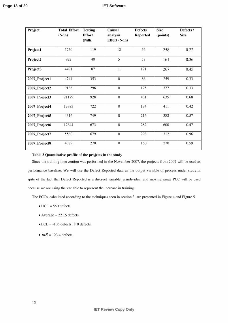
Table 3 shows the quantitative profile for the organization’s projects. Since defect and effort information is
sensitive for any company [48], this study effort unites are Normalized development hours (Ndh). Ndh is
calculated by dividing the total cost of the project between the cost of an hour of development. Likewise, size is
measured in the organization’s size unit.
Page 12 of 20
IET Review Copy Only
IET Software
13
Project Total Effort
(Ndh)
Testing
Effort
(Ndh)
Causal
analysis
Effort (Ndh)
Defects
Reported
Size
(points)
Defects /
Size
Project1 5750 119 12 56 258 0.22
Project2 922 40 5 58 161 0.36
Project3 4491 87 11 121 267 0.45
2007_Project1 4744 353 0 86 259 0.33
2007_Project2 9136 296 0 125 377 0.33
2007_Project3 21179 928 0 431 635 0.68
2007_Project4 13983 722 0 174 411 0.42
2007_Project5 4316 749 0 216 382 0.57
2007_Project6 12644 673 0 282 600 0.47
2007_Project7 5560 679 0 298 312 0.96
2007_Project8 4389 270 0 160 270 0.59
Table 3 Quantitative profile of the projects in the study
Since the training intervention was performed in the November 2007, the projects from 2007 will be used as
performance baseline. We will use the Defect Reported data as the output variable of process under study.In
spite of the fact that Defect Reported is a discreet variable, a individual and moving range PCC will be used
because we are using the variable to represent the increase in training.
The PCCs, calculated according to the techniques seen in section 3, are presented in Figure 4 and Figure 5.
• UCL = 550 defects
• Average = 221.5 defects
• LCL = -106 defects � 0 defects.
• mR = 123.4 defects
Page 13 of 20
IET Review Copy Only
IET Software

14
0.000
100.000
200.000
300.000
400.000
500.000
600.000
Figure 3 Run chart for the "Defects Reported"
(performance baseline)
0
50
100
150
200
250
300
350
400
450
Figure 4 Moving range chart for the variation in
the “Defects Reported”
Finally, according to the organizations’ measurement system, the cost of a defect is 5.5 Ndh, which includes
the cost of detecting and fixing the defect.
2. Deploy and Execute the process
This step implies that the organizations execute their production process for developing software. Costs for
the proposed ROI calculation are most likely to be incurred during this step. In the case of this study, costs taken
into account were: effort invested in training and causal analysis.
3. Evaluate Data Availability
Of the available 2008 projects, the selected for this study included only those whose resources had attended
the training intervention in the previous year. The resulting set is presented in Table 3.
As described in section 3, at least three data points are needed to establish a process run chart. As a result,
the condition can be evaluated affirmatively.
5. Establish New Limits of Control
New control limits are established by applying the statistical process control techniques seen in section 3.
Figure 5 depicts the control limits for the performance baseline.
• UCL = 165 defects
• Average = 78 defects
• LCL = - 8 defects � 0 defects
• mR = 32.5 defects
UCL Max
LCL
Page 14 of 20
IET Review Copy Only
IET Software

15
0.000
20.000
40.000
60.000
80.000
100.000
120.000
140.000
160.000
180.000
Project1 Project2 Project3
Figure 5 Run chart. “education defects
percentage” for 2008 projects
0.00
20.00
40.00
60.00
80.00
100.00
120.00
140.00
Project1 Project2 Project3
Figure 6 Moving range chart, “education defects
percentage” for 2008 projects
6. Calculate ROI
The costs for deploying and delivering the training were:
• CostCausalAnalysis = 27.9 Ndh
• CostTraining = 73.2 Ndh
Therefore: 101.1Cost Ndh=
Benefits are calculated by taking into account the process variation observed in both sections:
• DefectsExpected are represented by the control limits in Figure 3 and by the observed average.
Applying the method presented in 4.2 we calculate the expected defects for each of the cases:
o For the Worst case evaluation, DefectsExpected = LCLbaseline = 0 defects
o For the Observed case evaluation, DefectsExpected = Averagebaseline = 221.5 defects
o For the Best case evaluation, DefectsExpected = UCLbaseline = 550
• DefectsObserved
o In the best case, the LCL is calculated to be less than 0 defects. Thus, we take 1 defect as the
best case.
o The real case is observed average for the year 2008: 78 defects
o The worst case is the UCL for the year 2008 = 165 defects.
Cost of a defect. As it was mentioned in the first step, the organizational cost of a defect is 5.5
Ndh.Therefore ROI:
o ROI Worst case = -1007%
o ROI Observed case = 690%
o ROI Best case = 2935%
ROI for the training intervention was [-1007%, 2935%] with an observed case of 690% for a six month
period.
UCL
LCL
Max
Page 15 of 20
IET Review Copy Only
IET Software

16
6 Interpreting the results of the case study
In the previous section, we presented the case study of the application of the proposed method. Nevertheless,
it is still necessary to discuss the meaning of the range in the ROI results.
First, by presenting ROI results in range format, senior management can evaluate whether to repeat or not the
training intervention. Under the premise of process stability, senior management can assess the chances of
obtaining a favourable result of a future intervention.
The observed case, is the result that would have been obtained with the traditional ROI by averages
approach. It is the actual ROI for the intervention under study. As such, the value is subject to the specific
conditions (trainees, trainer, etc) that took place during the period under study and are not likely to be repeated.
This is to say, it does not account for variation. Therefore, future decisions based on this value alone are
oblivious to the risks that the worst case scenario represents.
On the other hand, the variation of the ROI results depends on the variation of the statistically controlled
process. Decisions with less uncertainty can be made with processes that are more stable (they exhibit narrower
variation around the mean value).
7 Threats to validity
In this section we acknowledge that major threats to validity for this case study are [49, 50]:
I. Internal validity
In reference to how were the data points collected (instrumentation validity), all data collected for this case
study were obtained directly from the organization measurement database. Only minor interventions were
needed in the organizational measurement system to support the data needed for this study (see [46, 47]).
II. Construction
According to experimental design types, the case study presented was constructed as an interrupted time
series quasi-experiment [51]. In these types of experiments, causality cannot be attributed to the independent
variable [49]. In this case the researchers judgement can be used to determine causal relationships which might
not stand the test of true experiments [52]. Interrupted time series design is built by a series of observations
before and after the intervention, so that changes in behaviour can be assigned to the intervention. The
disadvantage is that the environment is not under the researchers’ control. Interrupted time series quasi-
experiments are susceptible to the minimum number of data points needed to establish the measurement
Page 16 of 20
IET Review Copy Only
IET Software
17
baseline, and to gauge deviations after the interventions. In this case study, the available dataset might not be
able to support the conclusions about the effectiveness of the training intervention, but it does not invalidate the
applicability of the proposed ROI process.
On the other hand, subject selection for the case study was beyond the control of the researchers. The
managers assigned Project´s teams. The organization also selected which projects to deploy the causal analysis
process.
III. Conclusion
In spite of the available data points, we have taken care to abide by the statistical rules and preconditions of
the applied SPC techniques. As a result, the descriptive ability of the proposed ROI calculation is subject to the
same limitations as the techniques that it uses.
IV. External
We believe that the method can be applied in organizations that comply with its preconditions (Step 0
presented in section 4.1. It is also noteworthy that the selection of projects, and the ability of the organization to
provide a baseline of projects data is key if the proposal is to be replicated in another environment.
The interrupted time series case study can also be replicated.
8 Conclusion
In this paper, we have presented how it is possible to take into consideration the natural process variation of
the production process when calculating return on training investment. The presented method takes advantages
of statistical process control techniques to account for the variation in ROI on training calculations.
We expect that this method will provide training and senior management with a better tool for understanding
the contribution of the training efforts to the organization. A ROI presented using ranges enables managers to
evaluate risks associated to repeating a training intervention. Since the range allows them to see all possible ROI
of the intervention (in contrast to a unique number given by a calculation of ROI in averages).
The observed case, though it is still important because it is the ROI that the organization achieved in this
specific instance, cannot be used alone to determine whether the same intervention con be repeated with
success.
The presented method was experimented at a software factory and the results of the case study showed the
applicability of the proposal. In the case study, the organization obtained a ROI range of [-1007%, 2935%] with
an observed case of 690% for a six month period.
Page 17 of 20
IET Review Copy Only
IET Software
18
9 Acknowledges
The authors would like to thank the chair IBM-Rational of the Universidad Politécnica de Madrid for
supporting this work.
10 Bibliography
1 Chrissis, M.B., Konrad, M., and Shrum, S. CMMI : Guidelines for Process Integration
and Product Improvement. (Second). Upper Saddle River, NJ: Addison-Wesley: 2007.
2 International Standards Organization. ‘ISO 9001:2000(E). Quality Management
Systems - Requirements’. 2000.
3 International Standards Organization. ‘ISO/IEC 15504-1:2004 Information
technology Process assessment Part 1: Concepts and vocabulary’. 2004.
4 Murugappan, M., and Keeni, G. ‘Quality improvement-the Six Sigma way’.
Proceedings of, 2000 248-257.
5 El Emam, K., and Garro, I. ‘Estimating the extent of standards use: the case of
ISO/IEC 15504’, The Journal of Systems & Software, 53, (2), (2000). pp. 137-143.
6 Alliger, G.M., and Janak, E.A. ‘Kirckpatrick's Levels of Training: Thirty years later’,
Personnel Psychology, 42, (2), (1989). pp. 331-342. doi:10.1111/j.1744-6570.1989.tb00661.x
7 Phillips, J.J. Return on Investment in Training and Performance Improvement
Programs, Second Edition (Improving Human Performance). Butterworth-Heinemann:
2003.
8 Glover, R.W., and University of Texas at, A. Return-on-investment (ROI) Analysis of
Education and Training in the Construction Industry. Center for Construction Industry
Studies: 1999.
9 Van Solingen, R. ‘Measuring the ROI of software process improvement’, Software,
IEEE, 21, (3), (2004). pp. 32-38.
10 Shewhart, W. Economic Control of Quality of Manufactured Product. American
Society for Quality: 1980.
11 David, N.C., Kevin, D., and Glyn, D. ‘Making Statistics Part of Decision Making in
an Engineering Organization’, IEEE Softw., 25, (3), (2008). pp. 37-47.
http://dx.doi.org/10.1109/MS.2008.66
12 Zangwill, W.I., and Kantor, P.B. ‘Toward a theory of continuous improvement and
the learning curve’, Management Science, 44, (7), (1998). pp. 910-920.
13 Ruona, E.A., Leimbach, M., Holton Iii, F., and Bates, R. ‘The relationship between
learner utility reactions and predicted learning transfer among trainees’, International Journal
of Training and Development, 6, (4), (2002). pp. 218-228.
14 Hodges, T. Linking Learning and Performance. Masachusetts: Butterworth
Heinmann: 2002.
15 Kirkpatrick, D. ‘Four-level training evaluation model’, US Training and Development
Journal, (1959). pp.
16 Kirkpatrick, D.L., and Kirkpatrick, J.D. Evaluating Training Programs: The Four
Levels. (3rd). Berrett-Koehler Publishers: 2006.
Page 18 of 20
IET Review Copy Only
IET Software
19
17 Wang, G.G., and Wilcox, D. ‘Training Evaluation: Knowing More Than Is Practiced’,
Advances in Developing Human Resources, 8, (4), (2006). pp. 528-539.
18 Alliger, G.M., Tannenbaum, S.I., Bennett, W., Traver, H., and Shotland, A. ‘A Meta-
Analysis of the Relations among training criteria’, Personnel Psychology, 50, (2), (1997). pp.
341-358
19 Shelton, S., and Alliger, G. ‘Who's Afraid of Level 4 Evaluation? A Practical
Approach’, Training and Development, 47, (6), (1993). pp. 43-46.
20 Wang, G.G., Dou, Z., and Li, N. ‘A systems approach to measuring return on
investment for HRD interventions’, Human Resource Development Quarterly, 13, (2),
(2002). pp.
21 Holton, E.F., III. ‘The flawed 4-level evaluation model’, Human.
RusirurceDmelopment Quarterly, 7 (1), (1996). pp. 5—2.
22 Andrews, T.L., and Crewe, B.D. ‘Examining training reactions, lessons learned,
current practices and results’, Rogelberg, S. Informed decisions: Research-based practice
notes. TIP The organizational-industrial psychologist, 36, (4), (1999). pp.
23 Ilian, H. ‘Levels of Levels: Making Kirkpatrick Fit the Facts and the Facts Fit
Kirkpatrick’, Proceedings of the 6 thAnnual Human Services Training, (2004). pp.
24 Wang, G.G., and Spitzer, D.R. ‘Human Resource Development Measurement and
Evaluation: Looking Back and Moving Forward’, Advances in Developing Human Resources
7, (5-15), (2005). pp.
25 Swanson, R.A., and Holton, E.F. Foundations of Human Resource Development. (2nd
Edition). Berrett-Koehler Publishers: 2009.
26 Russ-Eft, D., and Preskill, H. ‘In search of the Holy Grail: return on investment
evaluation in human resource development’, Advances in Developing Human Resources, 7,
(1), (2005). pp. 71.
27 Card, D. ‘Building a Business Case for Process Improvement’. Proceedings of Europe
SEPG, 2008.
28 Boehm, B. ‘Value-based software engineering: reinventing’, SIGSOFT Softw. Eng.
Notes, 28, (2), (2003). pp. 3. 10.1145/638750.638775
29 Humphrey, W.S. Winning with Software: An Executive Strategy. Addison-Wesley
Professional: 2001.
30 Herbsleb, J., Carleton, A., Rozum, J., Siegel, J., and Zubrow, D. Benefits of CMM-
Based Software Process Improvement: Initial Results. Inst Carnegie-Mellon Univ Pittsburgh
Pa Software Engineering. Carnegie Mellon University, Software Engineering Institute. 1994.
31 Diaz, M., and Sligo, J. ‘How Software Process Improvement Helped Motorola’, IEEE
Software, (1997). pp.
32 van Solingen, R. ‘Measuring the ROI of software process improvement’, 21, (3),
(2004). pp. 32-38.
33 Humphrey, W.S. Introduction to the Team Software Process. Addison-Wesley
Professional: 1999.
34 Deming, W.E. Out of the Crisis. (First). Cambridge, Massachusetts: MIT Press:
2000.
35 Shewhart, W.A. Economic control of quality of manufactured product. Milwaukee,
Wis.: American Society for Quality Control: 1980.
36 Goldenson, D.: ‘The State of Software Measurment Practice’. Proc. Europe SEPG 08,
Munich, Germany, 12-14 June 2008 pp. Pages
37 Radice, R. ‘Survey Results of Baselines and Models Used by Level 4 and 5
Organizations’. Proceedings of SEPG 2010, 2010.
38 Wheeler, D.J. Understanding Variation: The Key to Managing Chaos. (Second
Revised Edition). Knoxville, Tennessee: Spc Press Inc.: 1993.
Page 19 of 20
IET Review Copy Only
IET Software

20
39 Florac, W.A., Park, R.E., and Carleton, A.D. Practical Software Measurement:
Measuring for Process Management and Improvement. Software Engineering Institute. 1997.
CMU/SEI-97-HB-003.
40 Adler, P.S., and Clark, K.B. ‘Behind the learning curve: a sketch of the learning
process’, Management Science, (1991). pp. 267-281.
41 Raccoon, L.B.S. ‘A learning curve primer for software engineers’, ACM SIGSOFT
Software Engineering Notes, 21, (1), (1996). pp. 86.
42 Matalonga, S., and SanFeliu, T. ‘Linking Return on Training Investment with Defects
Causal Analysis’. Proceedings of 20th Conference of Software Engineering Theory and
Practice, 2008 42-47.
43 Basili, V.R. Software modeling and measurement: the Goal/Question/Metric
paradigm. University of Maryland. 1992. CS-TR-2956, UMIACS-TR-92-96.
44 Pyzdek, T. The Six Sigma Handbook: The Complete Guide for Greenbelts,
Blackbelts, and Managers at All Levels. (Second Edition). McGraw-Hill: 2003.
45 Dettmer, W. The Logical thinking process: a systems approach to complex problem
solving. Milwakee. USA: American Society for Quality: 2007.
46 Matalonga, S., and Feliu, T.S. ‘Using defect data to drive Organizational Training
efforts’. Proceedings of International Conference on Software Engineering Theory and
Practice, 2008 61-68.
47 Matalonga, S., and San Feliu, T. ‘Defect Driven Organizational Training’.
Proceedings of Europe SEPG 2008, 2008.
48 Mizukami, D.: ‘Analyzing Defects Can Tell a LOT About a Company’. Proc. SEPG
Conference 2007, March 26 - 29, 2007 2007 pp. Pages
49 Campbell, D.T., and Stanley, J.C. ‘Experimental and quasi-experimental designs for
research on teaching’, Rand McNally, London, (1963). pp.
50 Wohlin, C., Höst, M., Runeson, P., Ohlsson, M.C., Regnell, B., and Wesslén, A.
Experimentation in software engineering: an introduction. Norwell, Massachusetts: Kluwer
Academic Publishers: 2000.
51 Field, A., and Hole, G. How to Design and Report Experiments. (7). Los Angeles,
California: SAGE Publishing: 2003.
52 Glass, G., and Jager, R.M. ‘Interrupted Time Series Quasi-Experiments’:
‘Complementary methods for research in education’ (American Educational Research
Association, 1997)
Page 20 of 20
IET Review Copy Only
IET Software