cal/apt program comparison of caltrans and aashto pavement design … of ct and aashto.pdf ·...

CAL/APT PROGRAM ─ COMPARISON OF CALTRANS AND

AASHTO PAVEMENT DESIGN METHODS

Report Prepared for

CALIFORNIA DEPARTMENT OF TRANSPORTATION

by

John Harvey and Fenella Long

September 1999Pavement Research Center

Institute of Transportation StudiesUniversity of California, Berkeley

iii

TABLE OF CONTENTS

List of Tables................................................................................................................................... v

List of Figures ...............................................................................................................................vii

Disclaimer ...................................................................................................................................... ix

Financial Disclosure Statement ...................................................................................................... ix

Implementation Statement.............................................................................................................. ix

Acknowledgements ........................................................................................................................xi

Executive Summary ........................................................................................................................ 1

1.0 Introduction ............................................................................................................................. 5

1.1 Objectives............................................................................................................................ 5

1.2 Overview of Report ............................................................................................................. 8

2.0 Summary of Design Methodologies........................................................................................ 9

2.1 AASHTO Design Procedure ............................................................................................... 9

2.2 Caltrans Design Procedure ................................................................................................ 12

3.0 Thickness DEsign Matrix...................................................................................................... 15

3.1 Traffic................................................................................................................................ 15

3.2 Pavement Materials ........................................................................................................... 17

3.2.1 Subgrade.................................................................................................................... 17

3.2.2 Subbase...................................................................................................................... 17

3.2.3 Aggregate Base.......................................................................................................... 18

3.2.4 Asphalt Concrete ....................................................................................................... 19

3.3 Reliability .......................................................................................................................... 20

3.4 Costs and Economic Selection of Thicknesses ................................................................. 20

iv

4.0 Thickness DEsign Comparison ............................................................................................. 23

4.1 Design Selection Criteria for This Experiment ................................................................. 23

4.2 Thickness Designs, Results, and Analysis ........................................................................ 25

4.2.1 Effect of Subbase Modulus on Thickness and Structural Equivalency of AASHTO

Designed Pavements ............................................................................................................. 26

4.2.2 Pavement Thicknesses and Structural Equivalency. ................................................. 29

4.2.3 Consideration of Drainage in AASHTO Procedure .................................................. 34

5.0 Fatigue Life Predictions ........................................................................................................ 37

5.1 UCB Design and Analysis Method ................................................................................... 37

5.2 Fatigue Life Predictions .................................................................................................... 41

6.0 Conclusions and Recommendations...................................................................................... 57

6.1 Summary ........................................................................................................................... 57

6.2 Conclusions ....................................................................................................................... 57

6.3 Recommendations ............................................................................................................. 61

7.0 References ............................................................................................................................. 65

v

LIST OF TABLES

Table 3.1 Thickness design matrix of pavement structures ...................................................... 16

Table 3.2 Traffic Index Values and Corresponding ESALs...................................................... 16

Table 3.3 Aggregate Moduli and Structural Coefficient ........................................................... 19

Table 4.1 Effect of aggregate subbase modulus on layer thickness and gravel equivalent

(AASHTO procedure) ........................................................................................................... 27

Table 4.2 Summary of pavement layer thicknesses for Caltrans “lowest cost,” Caltrans

“thinnest asphalt concrete,” and AASHTO designs.............................................................. 30

Table 4.3 Effect of drainage coefficient on thickness, structural number, and gravel equivalent

(AASHTO procedure) ........................................................................................................... 34

Table 5.1 Temperature conversion factors and shift factors ..................................................... 43

Table 5.2 Predicted pavement fatigue lives for Caltrans “lowest cost,” Caltrans “thinnest

asphalt concrete” and AASHTO designs, assuming 90-percent reliability........................... 44

Table 5.3 Ratios of predicted pavement fatigue lives for Coastal and Valley asphalt mixes. .. 51

Table 5.4 Ratios of predicted pavement fatigue lives for Caltrans “lowest cost,” Caltrans

“thinnest asphalt concrete” and AASHTO designs............................................................... 54

vii

LIST OF FIGURES

Figure 4.1 Structural numbers (SN) for pavements designed by Caltrans and AASHTO

procedures. ............................................................................................................................ 31

Figure 4.2 Gravel equivalents (GE) for pavements designed by Caltrans and AASHTO

procedures. ............................................................................................................................ 32

Figure 5.1 Summary of elements of UC Berkeley fatigue analysis and design procedure......... 39

Figure 5.2 Comparison of predicted fatigue performance for pavements designed by Caltrans

and AASHTO procedure, TI = 7 (linear plot) ....................................................................... 45


and AASHTO procedure, TI = 9 (linear plot) ....................................................................... 46


and AASHTO procedure, TI = 11 (linear plot) ..................................................................... 46






and AASHTO procedure, Valley asphalt mixes (logarithmic plot) ...................................... 48


and AASHTO procedure, Coastal asphalt mixes (logarithmic plot)..................................... 49

ix

DISCLAIMER

The contents of this report reflect the views of the authors who are solely responsible for

the information and the accuracy of the data presented herein. The contents do not necessarily

reflect the official views or policies of the California Department of Transportation (Caltrans) or

the Federal Highway Administration. This report does not constitute a standard, specification, or

regulation.

FINANCIAL DISCLOSURE STATEMENT

This research has been funded by the Division of New Technology and Research of the

State of California Department of Transportation (contract No. RTA-65W485). The total

contract amount for the five-year period (1 July 1994 through 30 June 1999) is $5,751,159. This

contract was later amended to extend to 30 June 2000 in the amount of $12,804,824.

This report presents the results of an investigation comparing pavement structures

designed with the Caltrans and AASHTO design methods, and performance predictions for both

sets of designs. The report presents an analysis of the results and conclusions with implications

for Caltrans pavement design practices. It also presents a plan for an improved pavement design

method based on mechanistic-empirical procedures.

IMPLEMENTATION STATEMENT

The results of the analyses presented in this report indicate that the Gravel Factors for

asphalt concrete included in the current Caltrans flexible pavement design method should be re-

evaluated. The Gravel Factors should probably be adjusted to provide thicker asphalt concrete

layers, especially for pavements expected to carry large volumes of truck traffic. Implementation

x

of new Gravel Factors that result in thicker asphalt concrete layers should significantly improve

the performance of heavy-duty pavements and result in reduced maintenance costs and longer

periods between required rehabilitations. Re-calculation of Gravel Factors requires a database

containing pavement structure and performance data, which Caltrans currently doesn’t have.

This indicates either the need for a mechanistic-empirical design method, or waiting years to

develop an adequate database.

The current Caltrans flexible pavement design method treats asphalt concrete as a generic

material. Simulations of pavement performance reported herein indicate significant differences

in predicted fatigue life depending upon asphalt concrete mix. Movement from the current

empirical design method to a mechanistic-empirical method is recommended based on these and

other analyses in this report. Implementation of a mechanistic-empirical design method will

result in better estimation of pavement performance by taking into account materials selection,

layer thickness, subgrade strength, drainage, and loading characteristics that cannot be included

in the current method. Use of a mechanistic-empirical method should result in significant

improvements in pavement design, including savings from selection of more economical

combinations of materials and layer thicknesses, and improved programming of maintenance and

rehabilitation funds from better estimates of pavement performance. A plan for implementation

of a mechanistic-empirical design method is included in this report.

The current Caltrans design method assumes that inclusion of positive drainage systems,

including treated permeable base, edge drains, and outlets, will improve pavement performance.

Results presented in a separate CAL/APT report on inclusion of asphalt treated permeable base

in flexible pavements indicate that this may not always be the case. The effects of drainage

should be directly investigated by means of laboratory testing at different levels of saturation and

xi

included in the pavement design method. A mechanistic-empirical design method will facilitate

inclusion of this drainage information in the design method. These results should be included in

the design method software as well. Similarly, lifecycle cost calculations are required for most

Caltrans pavement designs, and should be included in the design software. The current software

(NEWCON90) only calculates initial construction cost. These changes will result in better

calculations of pavement performance and lifecycle cost.

ACKNOWLEDGEMENTS

Financial support for this project was provided by the State of California Department of

Transportation as part of the CAL/APT Project. Mr. Wesley Lum of the Division of New

Technology and Research is the CAL/APT Project Manager and Mr. William Nokes, Office of

Project Planning and Design, was the Contract Monitor for the University of California, Berkeley

during preparation of most of this report. Mr. Jeff Pizzi of the Division of New Technology and

Research was the Contract Monitor during the final stages of report preparation.

1

EXECUTIVE SUMMARY

This report compares the Caltrans and AASHTO pavement thickness design procedures.

The design comparisons include pavement structures subjected to a range in traffic, as

represented by Traffic Indexes of 7, 9, 11, 13, and 15, and a range in subgrade strengths, as

measured by subgrade R-values of 5, 20, and 40.

This report has four objectives:

1. Quantify the differences in pavement thickness resulting from use of the two methods.

2. Examine differences in predicted pavement performance for pavement designs

considered equal within the Caltrans method. Related to this objective is the

examination of the Gravel Factors for aggregate base and asphalt concrete.

3. Evaluate the effect of assumed drainage conditions on the pavement structures

designed using the AASHTO method and relate this effect to the Caltrans method.

4. Demonstrate the flexibility of the mechanistic-empirical design procedure developed

as part of the CAL/APT program to quantitatively, systematically, and rationally

permit pavement designers to evaluate the performance of different pavement

structures and different materials.

This report illustrates that the AASHTO and Caltrans pavement thickness design

procedures do not produce the same pavement structures for the same given inputs. The design

procedures are based on different material properties determined in the laboratory: The Caltrans

procedure uses the R-value test and AASHTO uses the resilient modulus test (MR). Generally,

the pavement structures designed by the Caltrans procedure are thicker than those designed by

the AASHTO procedure. This increase in thickness results in improved fatigue performance for

the pavement designed according to the Caltrans procedure. The fatigue performance of the

2

pavements is extremely sensitive to the asphalt concrete thickness. In this report, it is shown that

due to the differences between the design procedures they should not be used interchangeably. It

is also shown that for the subbase, the procedures are sensitive to the conversion from one type

of laboratory test to another.

The relative contribution of asphalt concrete, granular base, and subbase materials to a

pavement structure’s load carrying capability is different for the two design procedures. Results

presented indicate that the structural contribution of the asphalt concrete to fatigue cracking

resistance for thicker asphalt concrete layers is larger than indicated by the Caltrans Gravel

Factors. It is therefore recommended that the Gravel Factors for asphalt concrete be re-evaluated.

The predicted fatigue performance of two Caltrans design options, “lowest cost” and

“thinnest asphalt concrete layer allowed,” are significantly different for most inputs of Traffic

Index (TI) and subgrade R-value. It is therefore likely that pavements designed using the

Caltrans procedure, which are supposed to have similar performance as measured by the Gravel

Equivalent (GE), will exhibit different fatigue performance: Thicker asphalt concrete layers will

exhibit better performance than thinner asphalt concrete layers.

Considerations of pavement drainage and lifecycle cost analyses are included in the

AASHTO procedure but not in the Caltrans procedure. The Caltrans procedure assumes that

pavement designs without special drainage priorities are adequate and that their inclusion makes

Caltrans pavement designs conservative. Both drainage conditions and lifecycle cost analyses

should be explicitly included in the Caltrans design method.

Predicted pavement performance is also sensitive to different asphalt concrete mixes.

Two mixes were evaluated with AR-4000 binders, one from a California Valley source and the

3

other from a California Coastal source. The California Coastal binder performed better in all the

structures analyzed.

Using the University of California Berkeley fatigue analysis and design procedure, the

fatigue performance predictions suggest that the Caltrans “lowest cost” pavements are adequate

at a 90-percent reliability level for all Traffic Indices and subgrade R-values of 20 and 40.

However, for a subgrade R-value of 5, the Caltrans “lowest cost” pavement designs may not be

adequate. Moreover, the results indicate that all Caltrans “thinnest allowable asphalt concrete

layer” designs are likely not adequate at the 90-percent reliability level. It would also appear that

AASHTO pavement designs may not be adequate at this reliability level. Substitution of the

Coastal asphalt mix for the Valley asphalt mix did not change these conclusions.

This report demonstrates the ability of the mechanistic-empirical pavement analysis and

design procedure to quantitatively evaluate the effects of pavement structure, materials selection,

and subgrade strength on a specific mode of pavement distress. It is recommended that Caltrans

move towards implementation of a mechanistic-empirical fatigue analysis and design procedure

for the design of asphalt concrete pavements. An implementation procedure is recommended.

5

1.0 INTRODUCTION

The majority of state highway agencies in the United States use flexible pavement design

procedures that are essentially empirical, i.e., determination of the structural equivalencies of

pavement materials and selection of thicknesses of the pavement components are based on

observed performance of pavements. As conditions change, the procedures are modified to

reflect these changes. Many state highway agencies use the design procedure originally

developed from results of the American Association of State Highway Officials (AASHO) Road

Test. (1) That procedure, expanded and updated at regular intervals, is now referred to as the

American Association of State Highway and Transportation Officials (AASHTO) procedure

following the name change of the organization. The California Department of Transportation

(Caltrans) also uses an empirical pavement design method. Although both methods are

empirically based, for the same inputs of materials and traffic they result in pavements with

different thicknesses.

Because of the direct correlation of pavement thickness and traffic, it should be expected

that empirical design procedures developed from different databases would produce different

performances when variables that are not design inputs are different. These variables include,

but are not limited to, different environmental conditions and different subgrade soils.

1.1 Objectives

The first objective of this report is to quantify the differences in pavement thickness

resulting from use of the Caltrans and AASHTO methods. Bases for this objective include the

following:

6

1. Illustration of the limitations of design procedures when used for a wide variety of

variables affecting pavement performance. For example, if there are differences

between structures designed with a procedure based on environmental conditions in

Illinois (AASHTO) and a procedure based on California conditions, there should also

be differences for the wide range of environments found within California. This is

particularly important for flexible pavements, which rely on a temperature-sensitive

material such as asphalt concrete.

2. The range of performance observations contained in the two design methods provides

a reference against which mechanistic-empirical design procedures can be calibrated.

It is therefore important to quantify differences between those sets of observations.

Eventually, further calibration of the relationships between stresses and/or strains

calculated from models of the pavement structure (the mechanistic part of

mechanistic-empirical methods) and pavement performance should be made using

accelerated pavement tests and long-term pavement performance data.

3. Some engineers who are not well experienced in the pavements area may consider the

Caltrans and AASHTO empirical design procedures to be interchangeable and that

they should produce similar design thicknesses. At times this can lead to

disagreements as to a required design. For example, if a private toll road is designed

by the AASHTO method and is to be accepted by a California public agency that

typically uses Caltrans designs, that agency should expect differences in the

performance from the two methods. It is also important to quantify differences in

pavement designs produced by the two methods for different design conditions,

considering that both methods, and particularly the AASHTO method, involve

7

considerable extrapolation for traffic levels above a Traffic Index between about 11

and 12 (8,000,000 ESALs), and for more than a few subgrade soils types. (1)

The second objective is to examine differences in predicted pavement performance for

pavement designs considered equal within the Caltrans method. This objective permits

examination of the materials structural equivalencies, or Gravel Factors (GF), for the materials

considered in the Caltrans procedure. The performance predictions are made using the

mechanistic-empirical method for fatigue analysis and design developed by UCB for Caltrans.

(2)

The third objective is to evaluate the effect of assumed drainage conditions on pavement

structures designed using the AASHTO method. The Caltrans method assumes a worst case

scenario including poor drainage and a saturated subgrade as represented by the conditions for

the R-value test. Language within the Caltrans method indicates that pavement performance

should be improved by inclusion of drainage features in the pavement. (3) However, the method

provides no change in pavement thickness design when drainage features, such as edge drains

and drainage layers (typically asphalt treated permeable base [ATPB]), are included in the design.

The AASHTO method provides a rudimentary indication of the effect of inclusion of pavement

drainage features on pavement thickness design.

The fourth objective is to demonstrate the flexibility of mechanistic-empirical design

procedures to quantitatively, systematically, and rationally permit pavement designers to evaluate

the performance of different pavement structures and different materials. In this report, two

typical California asphalt mixes are included in the analyses as examples.

The ability of mechanistic-empirical procedures to permit Caltrans policy-makers to

evaluate the effects of potential changes in factors affecting pavement performance and

8

infrastructure investment needs is demonstrated. For example, although only one tire pressure

and axle wheel type (single axle, dual wheels, 690 kPa [100 psi] contact pressure) is included in

the analyses in this report, the same analyses to evaluate the effects of wide-base single wheels

(super singles) or changes in typical tire pressures (e.g., to 800 kPa [115 psi]) could be performed

in a short period of time. The introduction of new materials to Caltrans pavements can also be

quickly evaluated with some laboratory testing and the mechanistic-empirical procedure used in

this report.

Demonstrations of this approach have already been reported to Caltrans. These

demonstrations include evaluation of the effects of construction variables, such as asphalt

concrete compaction (2); use of ATPB as a structural material in flexible pavements under dry

and wet conditions (4); and development of rational QC/QA pay factors. (5)

1.2 Overview of Report

Chapter 2 of this report provides a brief discussion of the Caltrans and AASHTO design

methods, including fundamental concepts and some of the major assumptions. Chapter 3

discusses the thickness design matrix, including the assumed materials and the correlations

between the different materials classifications used by the two design procedures. Chapter 4

presents thickness designs resulting from the two procedures and predicts fatigue performance

for the sections using the thickness designs. Chapter 5 includes a summary and evaluation of the

analyses and recommendations resulting from the evaluation of the information.

It should be noted that the non-metric version of the Caltrans design procedure was used

for this study because the metric version was not yet available to UCB when this study was

begun. It is assumed that the results from the metric version will be approximately the same.

9

2.0 SUMMARY OF DESIGN METHODOLOGIES

Both the AASHTO (1) and the Caltrans (3) design methods are based on a similar

concept and are developed from empirical data. This section presents a brief overview of each

design method, key assumptions, and important differences as well as an indication of

similarities.

The concept on which both design procedures are based is that each layer (or material) is

characterized by a value representing its structural equivalency relative to the other layers. The

sum of the products of structural equivalencies and layer thicknesses gives a single number that

is used as a check to ensure that the pavement can adequately withstand the traffic demand for

the subgrade strength. AASHTO uses layer coefficients and the total pavement structural

capacity is referred to as the “Structural Number” (SN). Caltrans uses “Gravel Factors” (Gf) to

quantify structural equivalency and a “Gravel Equivalent” (GE) for the pavement structural

capacity.

2.1 AASHTO Design Procedure

The AASHTO procedure is based on performance data obtained from the AASHO Road

Test conducted in Ottawa, Illinois, from 1956 to 1960. Modifications have been made to

improve the design guide based on research completed and experience gained since the initial

implementation of the guide in 1972. Because the procedure was developed from one test track,

an important limitation is that the database is based on one set of materials, limited pavement

types, and limited loads and load types. Aging is limited and the environmental influences on the

data are limited to that specific environment. Detailed discussion of these factors and their

limitations is found in the AASHTO guide. (1)

10

The AASHTO method uses a Structural Number (SN) to represent the designed pavement

structure, and each layer is characterized by a structural coefficient (ai). The layer coefficients

were developed initially from performance information for the AASHO Road Test and then later

related to moduli and the associated stresses and strains produced by multi-layered pavement

analyses (similar to the UCB procedure).

The AASHTO procedure makes use of the empirically developed expression (Equation

2.1) to predict the amount of traffic that can be sustained before the pavement deteriorates to a

specified terminal level of serviceability, which can be chosen by the designer.

(2.1)

where W18 = predicted number of 18-kip (80kN) equivalent single axle load

applications (ESALs),

ZR = standard normal deviate,

S0 = combined standard error of the traffic prediction and performance

prediction,

∆ PSI = difference between the initial design serviceability index, p0, and the

design terminal serviceability index, pt, and

MR = resilient modulus (psi) of subgrade.

In order to balance equation 2.1, a Structural Number (SN) calculated as a function of

pavement layer thicknesses, must be selected as follows:

(2.2)

where ai = ith layer coefficient,

Di = Th layer thickness (inches) and

( ) ( )

( )

( ) 07.8log32.2

110944.0

5.12.4log

20.01log36.9log

19.5

018 −•+

++

−∆

+−+•+•= RR M

SN

PSI

SNSZW

33322211 mDamDaDaSN ++=

11

mi = ith layer drainage coefficient.

Determination of the demand traffic ESALs from the expected traffic loading on the

facility is obtained from tables of axle load equivalency factors which are a function of the axle

configuration and loads, structural number, and terminal serviceability (1). In a number of

instances, the equivalencies can be approximated by the expression:

(2.3)

where: WESAL = repetitions of an 80 kN single axle developing same pavement

damage as one repetition of a single axle with a load = Wload

(kN), and

n = approximately 4 for a range in loads.

This exponent is actually a function of pavement type and therefore changes in the

pavement type can have a significant effect on the pavement performance. Accordingly, it is

more appropriate to use the tables in Reference (1) to deference the exponent.

The AASHTO design procedure also incorporates reliability to account for some of the

risk factors involved in designing pavements., for example, the traffic prediction, material

variability, and construction variability. The method also accounts for seasonal variation of the

subgrade modulus.

The design process consists of selecting the layer thicknesses to obtain the Structural

Number required to obtain the required load applications (demand traffic). This process is begun

at the layer just above the subgrade and then repeated for each layer working towards the surface

of the pavement.

nload

ESALW

W ��

�=80

12

Lifecycle costs are calculated in the procedure and are used as the basis for selection of a

pavement structure from pavements with the same Structural Number.

2.2 Caltrans Design Procedure

The Caltrans design procedure (3) is based on theory, test track studies, experimental

sections, materials research, and empirical evidence. (6) Data obtained from the AASHO Road

Test were used to update the design method. (7, 8) The method references the structural

equivalency of each layer, called the Gravel Factor (Gf), to the aggregate subbase. The Gravel

Equivalent (GE) of the pavement is calculated using the relationship:

(2.4)

where dAB and dSB are the thicknesses of the aggregate base and subbase layers (in feet)

respectively, and GfAB is the Gravel Factor for the aggregate base. GEAC is calculated using the

following relationship:

(2.5)

(2.6)

where dAC is the asphalt concrete layer thickness (feet) and TI is the design Traffic Index. The

required GE for the pavement is determined from the expected traffic during the design life and

the R-value of the subgrade soil, as shown below:

(2.7)

In contrast to the AASHTO design procedure, the Caltrans design method first calculates

the thickness of the top layer and then works down layer by layer. The effect of drainage is not

directly incorporated, except that the design guide states that the inclusion of positive drainage (a

feet500for 67.5

5.0 .dTI

dGE AC

ACAC ≤=

( )feet500for

00.75.0

34

.dTI

dGE ACAC

AC ≤=

SBfABAC dGdGEGEAB

+•+=

( )RTIGE −••= 1000032.0

13

drainage layer) will probably result in the service life exceeding the design life. In the R-value

test, unbound soils and granular materials are tested in a near saturated condition. It is likely that

many materials do not reach this weakened condition in California pavement sections.

The Caltrans guide states that the pavement selection should be based on the most

economical design, considering the total lifecycle costs of the facility. The lifecycle costs should

include the initial cost, maintenance cost, and anticipated rehabilitation costs during the selected

lifecycle period. If the TI is greater than 10 (approximately 2,500,000 ESALs), then a total

lifecycle cost analysis must be performed, as detailed in the design manual. However, the

Caltrans design guide software program used to perform the pavement thickness calculations

only calculates initial cost and does not calculate lifecycle costs. (9)

It would be relatively simple for lifecycle costs to be incorporated into the calculations in

the Caltrans software. Doing so would enhance the use of the software and bring it into

agreement with the stated design procedure and policy of Caltrans included in the text of the

design guide.

Conversion of the traffic loading spectrum to ESALs is performed using the load

equivalence factor (Equation 2.3) with the exponent n equal to 4.2. The Caltrans exponent of 4.2

results in the Caltrans load equivalence being more sensitive than the AASHTO load equivalence

factors..

15

3.0 THICKNESS DESIGN MATRIX

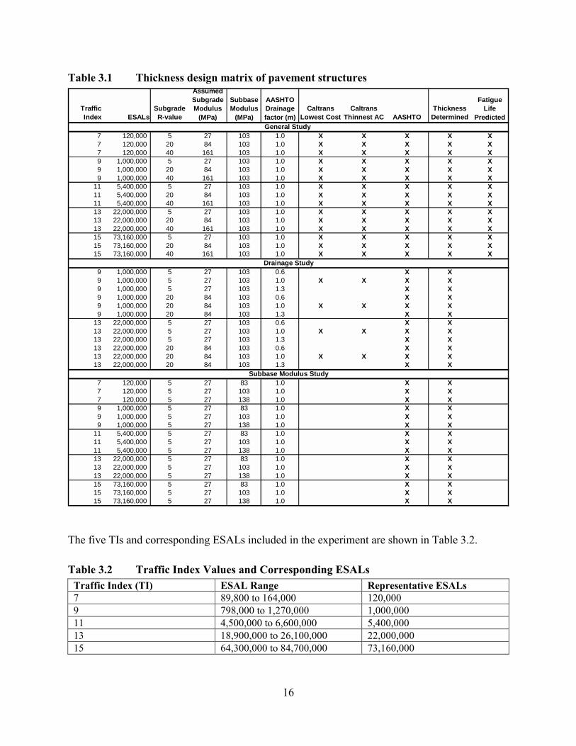
To compare the two design procedures, a thickness design matrix was established that

incorporated a number of variables, including traffic, materials, reliability, and cost. In this

section the variables used, the assumptions made, and the necessary conversions between the

different specifications associated with each design method are discussed.

The matrix utilized is summarized in Table 3.1. The first block contains the

combinations of traffic, materials, and drainage used to determine both pavement layer

thicknesses and fatigue life predictions. The second block summarizes the cases used in the

drainage study and the third block gives the cases used for determination of the effect of assumed

subbase modulus on pavement thickness in the AASHTO method.

3.1 Traffic

Five design traffic levels, shown below, are used in this study and span the range from

low to high levels of traffic on typical Caltrans highway pavements. The Caltrans design method

requires that the design traffic be described in terms of a Traffic Index (TI) and the AASHTO

design method requires equivalent standard axles (ESALs). The following equation from the

Caltrans design procedure (3) is used to convert between TI and ESALs:

(3.1)119.0

6100.9 �

��

�•= ESALTI

16

Table 3.1 Thickness design matrix of pavement structures

The five TIs and corresponding ESALs included in the experiment are shown in Table 3.2.

Table 3.2 Traffic Index Values and Corresponding ESALsTraffic Index (TI) ESAL Range Representative ESALs7 89,800 to 164,000 120,0009 798,000 to 1,270,000 1,000,00011 4,500,000 to 6,600,000 5,400,00013 18,900,000 to 26,100,000 22,000,00015 64,300,000 to 84,700,000 73,160,000

Traffic Index ESALs

Subgrade R-value

Assumed Subgrade Modulus

(MPa)

Subbase Modulus

(MPa)

AASHTO Drainage factor (m)

Caltrans Lowest Cost

Caltrans Thinnest AC AASHTO

Thickness Determined

Fatigue Life

PredictedGeneral Study

7 120,000 5 27 103 1.0 X X X X X7 120,000 20 84 103 1.0 X X X X X7 120,000 40 161 103 1.0 X X X X X9 1,000,000 5 27 103 1.0 X X X X X9 1,000,000 20 84 103 1.0 X X X X X9 1,000,000 40 161 103 1.0 X X X X X

11 5,400,000 5 27 103 1.0 X X X X X11 5,400,000 20 84 103 1.0 X X X X X11 5,400,000 40 161 103 1.0 X X X X X13 22,000,000 5 27 103 1.0 X X X X X13 22,000,000 20 84 103 1.0 X X X X X13 22,000,000 40 161 103 1.0 X X X X X15 73,160,000 5 27 103 1.0 X X X X X15 73,160,000 20 84 103 1.0 X X X X X15 73,160,000 40 161 103 1.0 X X X X X

Drainage Study9 1,000,000 5 27 103 0.6 X X9 1,000,000 5 27 103 1.0 X X X X9 1,000,000 5 27 103 1.3 X X9 1,000,000 20 84 103 0.6 X X9 1,000,000 20 84 103 1.0 X X X X9 1,000,000 20 84 103 1.3 X X

13 22,000,000 5 27 103 0.6 X X13 22,000,000 5 27 103 1.0 X X X X13 22,000,000 5 27 103 1.3 X X13 22,000,000 20 84 103 0.6 X X13 22,000,000 20 84 103 1.0 X X X X13 22,000,000 20 84 103 1.3 X X

Subbase Modulus Study7 120,000 5 27 83 1.0 X X7 120,000 5 27 103 1.0 X X7 120,000 5 27 138 1.0 X X9 1,000,000 5 27 83 1.0 X X9 1,000,000 5 27 103 1.0 X X9 1,000,000 5 27 138 1.0 X X

11 5,400,000 5 27 83 1.0 X X11 5,400,000 5 27 103 1.0 X X11 5,400,000 5 27 138 1.0 X X13 22,000,000 5 27 83 1.0 X X13 22,000,000 5 27 103 1.0 X X13 22,000,000 5 27 138 1.0 X X15 73,160,000 5 27 83 1.0 X X15 73,160,000 5 27 103 1.0 X X15 73,160,000 5 27 138 1.0 X X

17

3.2 Pavement Materials

The pavement structures used in this analysis are assumed to consist of an asphalt

concrete surface layer, an aggregate base, an aggregate subbase, and the subgrade. In some cases,

the aggregate subbase is eliminated because it is as strong as the subgrade or it is less than 150

mm (6 inches) thick. The materials used in the analysis are assumed to meet standard Caltrans

specifications. Because of different ways of defining materials response in the two methods, it is

necessary to convert materials properties between them in terms of results from their respective

reference tests: R-value for Caltrans and resilient modulus (MR) for AASHTO.

3.2.1 Subgrade

Three subgrades were used in the analysis, with R-values of 5, 20, and 40. These R-

values span a wide range in subgrade strength. Elastic moduli were estimated to be 27, 84, and

161 MPa (3,850, 12,200, and 23,400 psi) for R-values of 5, 20, and 40, respectively. (10) The

conversion included in the AASHTO design guide gives elastic moduli very close in magnitude

to the moduli assumed for this analysis.

3.2.2 Subbase

Only one subbase was used in this study, classified as a Class 2 aggregate subbase

according to Caltrans specifications. A Class 2 subbase has a minimum R-value of 50. The

Caltrans Gravel Factor for this material is 1.0. According to the AASHTO design guide, a

subbase with an R-value of 50 corresponds to a modulus of approximately 83 MPa (12,000 psi).

However, based on past experience, this modulus is considered too low for typical Caltrans

subbases and was adjusted to 138 MPa (20,000 psi). The conversions from R-value to modulus

18

in the AASHTO guide are averaged from correlations obtained in California, New Mexico, and

Wyoming; it was therefore considered acceptable to refine, based on experience with the HVS

test program, the moduli estimated from the AASHTO design guide to better reflect California

conditions. However, to ensure an equitable comparison between the Caltrans and AASHTO

thickness designs, three values of the subbase modulus were considered: 83, 103, and 138 MPa

(12,000; 15,000; and 20,000 psi). In the mechanistic-empirical prediction of fatigue life

presented in Chapter 5, a subbase modulus of 103 MPa (15,000 psi) is used.

The AASHTO method requires a structural coefficient, a function of modulus, as the

input for the material layers. For granular subbases, the following equation is used (1) where aSB

is the subbase structural coefficient and ESB is the subbase modulus (psi):

(3.2)

For the subbase moduli of 83, 103, and 138 MPa (12,000; 15,000; and 20,000 psi), the structural

coefficients are 0.09, 0.11, and 0.14, respectively.

3.2.3 Aggregate Base.

The aggregate base is assumed to meet the requirements of a Caltrans Class 2 aggregate

base. This base has a minimum R-value of 78. The Caltrans Gravel Factor is 1.1. Based on past

experience, (2) the modulus of the base is assumed to depend in part on the asphalt concrete

thickness as shown in Table 3.3. The AASHTO structural coefficient for the base is also shown

in Table 3.3 and is determined using the following equation where aAB is the structural coefficient

and EAB is the aggregate base modulus (psi). (1)

(3.3)

( ) 839.0log227.0 10 −= SBSB Ea

( ) 997.0log249.0 10 −= ABAB Ea

19

Table 3.3 Aggregate Moduli and Structural Coefficient

Class 2 Aggregate BaseAsphalt ConcreteThickness Elastic modulus AASHTO Structural Coefficient90 to 183 mm 207 MPa (30,000 psi) 0.14195 to 305 mm 172 MPa (25,000 psi) 0.12305 to 396 mm 138 MPa (20,000 psi) 0.09

3.2.4 Asphalt Concrete

Two asphalt concrete materials were included in the experiment with stiffnesses taken

from laboratory flexural beam test measurements. Both mixes included Watsonville granite

aggregate with a gradation between the Caltrans medium and coarse 19-mm specifications. (2)

The two asphalts both met AR-4000 specifications and were refined from California Coastal and

California Valley sources. For the two mixes, relationships were developed from laboratory

testing to estimate the stiffness of the mix for different air-void and asphalt contents. (2,11,12)

These relationships for a 20° Celsius test temperature and 10-Hz sinusoidal loading are:

(3.4)

(3.5)

where ln is the natural logarithm, S0 = initial flexural stiffness (MPa), and AC and AV are the

asphalt content and air-void content (percent), respectively. For the mix with the Coastal asphalt,

asphalt content was found to be statistically insignificant. Using these equations and an assumed

air-void content of 8 per cent (about 96 percent relative compaction in the Caltrans standard test

method CTM 304), and an assumed asphalt content of 5 percent by mass of aggregate, the Valley

mix has a stiffness of approximately 6,760 MPa and the Coastal mix a value of approximately

1,900 MPa. The 5-percent asphalt content is approximately that which meets the Hveem mix

design requirements for a minimum stability of 37 or minimum air-void content of 4 percent for

Caltrans standard laboratory compaction (standard test method CTM 367).

AVACSeWatsonvillValley 076.0172.0282.10ln:/ 0 −−=

AVSeWatsonvillCoastal 12224.05270.8ln:/ 0 −=

20

Using the guideline in the AASHTO design manual, the asphalt concrete stiffnesses of

1,900 MPa and 6,760 MPa correspond to structural coefficients of approximately 0.35 and 0.42,

respectively. For this analysis, the pavements were designed using a structural coefficient of 0.42

for the asphalt concrete; however, the mechanistic-empirical analysis component of the study

utilizes the actual stiffnesses.

3.3 Reliability

The AASHTO method permits explicit input of the desired design reliability in the

thickness design of the pavements. For this analysis, a reliability of 90 percent was used. The

Caltrans method does not permit input of the design reliability; however, it is certain that some

level of reliability must be implicitly included in the thickness design procedure. (13)

3.4 Costs and Economic Selection of Thicknesses

Both the Caltrans and AASHTO design procedures require unit costs for the materials.

The unit costs selected for use in both procedures were arbitrarily taken from the default costs of

the Caltrans procedure and are as follows: asphalt concrete, $70 per cubic yard; aggregate base,

$35 per cubic yard; and aggregate subbase, $25 per cubic yard. (9) All are in-place values.

For the Caltrans procedure, determination of the most economic pavement is made by

choosing the pavement structure with the lowest initial cost, an output of the software program.

The AASHTO design software presents only one pavement thickness, which is based on an

economic choice. The AASHTO software also permits the incorporation of lifecycle costs for a

specified design period. However, to facilitate a fair comparison between the Caltrans and

AASHTO procedures for this analysis, the interest rate was input as zero for the AASHTO

21

software in order to prevent the calculation of the full lifecycle costs. This was done because the

full lifecycle costs are not calculated in the Caltrans method.

The AASHTO method automatically selects the most economical design. However, if

the ratio of costs between the top two layers is smaller than the ratio between the structural

coefficients of the top two layers times the drainage coefficient, then the design selected is that

with the minimum base thickness as the optimum economic alternative.

23

4.0 THICKNESS DESIGN COMPARISON

Two software programs were used to determine the thicknesses: NEWCON90 (9), the

July 1990 version of Chapter 600 of the Caltrans Highway Design Manual (3); and, DNPS86

(14), the AASHTO design of New Pavement Structures Program, Version 1C, September 1986

(1).

4.1 Design Selection Criteria for This Experiment

A total of 90 pavements were designed using both the Caltrans and AASHTO procedures.

For the Caltrans procedure, two thickness designs were selected:

• for 30 pavements, the design with the Caltrans “thinnest allowable asphalt concrete

layer” was chosen (referred to as “thinnest asphalt concrete”), and

• for another 30 pavements, the lowest default cost design based on the default

materials costs mentioned in Section 3.4 was chosen (referred to as “lowest cost”).

For some of the cases, the Caltrans “thinnest asphalt concrete” design and the Caltrans

“lowest cost” design were identical. The thicknesses for the remaining 30 pavements were

designed according to the AASHTO procedure, which selects the lowest cost design.

Several rules were used for thickness selection in this analysis. The subbase was

eliminated if the thickness is less than 105 mm (4.2 inches). This is the default minimum

subbase thickness in the NEWCON90 program. A minimum aggregate base thickness of 150

mm (6 inches) was assumed due to the difficulties in constructing a base layer thinner than 150

mm.

The specified thicknesses were rounded to the nearest 0.05 ft., the unit in which Caltrans

specifies pavement layer thicknesses.

24

A shortcoming of the AASHTO software in this analysis is that if the program specifies

an aggregate base thickness less than the minimum (150 mm) and the thickness is manually reset

to 150 mm, neither the subbase nor the asphalt concrete thickness is decreased to compensate for

the increased base thickness. This occurred in a few of the cases.

Water infiltration in a pavement can severely affect performance by causing stiffness

reduction in the pavement layers, particularly the unbound layers. Accelerated damage results

from the reduced stiffness of these components; drainage, on the other hand, can reduce the

potential for damage. Therefore, drainage has an important influence on pavement performance

and should be taken into account by the design method. The AASHTO design procedure allows

the consideration of drainage whereas the Caltrans procedure does not. However, the R-value

test, a soaked test, is used to evaluate subgrade and other unbound soils materials and therefore

the materials are conservatively characterized.

The criteria that are considered in the AASHTO procedure for drainage are the time

within which the water will be removed from the pavement structure and the percent time the

pavement structure is exposed to moisture levels approaching saturation. These drainage

considerations are incorporated into the calculation of the Structural Number (SN) by applying a

drainage coefficient (m), as shown in the following relationship:

(4.1)

where SN = Structural Number,

ai = structural coefficients, and

Di = layer thicknesses.

The drainage coefficient is determined from the AASHTO design guide.

33322211 mDamDaDaSN ++=

25

For most of the analyses included in this study, the drainage coefficient was assumed to

be 1.0 for all layers. To investigate the effect of incorporating the drainage considerations into

the thickness designs of the AASHTO pavements, four of the pavement structures were

evaluated by varying the drainage inputs. The cases used for this small analysis are the TI 9 and

13 and R-value 5 and 20 cases, shown in Table 3.1. For both the base and the subbase, two

drainage coefficients were used. In the first, the pavement drainage was assumed to be good,

which means the water drains in one day and the pavement is exposed to moisture levels

approaching saturation less than 1 percent of the time. The drainage coefficient for this scenario

is 1.30. The second scenario assumed the pavement drainage was poor; for these conditions, the

water is assumed to take 1 month to drain and the pavement is exposed to moisture levels

approaching saturation more than 25 per cent of the time. The drainage coefficient for this

scenario is 0.60.

The cases used for this small analysis are the TI 9 and 13 and R-value 5 and 20 cases,

given in Table 3.1.

4.2 Thickness Designs, Results, and Analysis

The results from the thickness designs are presented and discussed in this section. Firstly,

the effect of the selected subbase modulus on the thickness of the pavements designed by the

AASHTO method is discussed; secondly, the pavement thicknesses from the AASHTO and

Caltrans design procedures are compared; and thirdly, the structural coefficients (AASHTO) and

Gravel Equivalents (GE) of the pavements are compared.

26

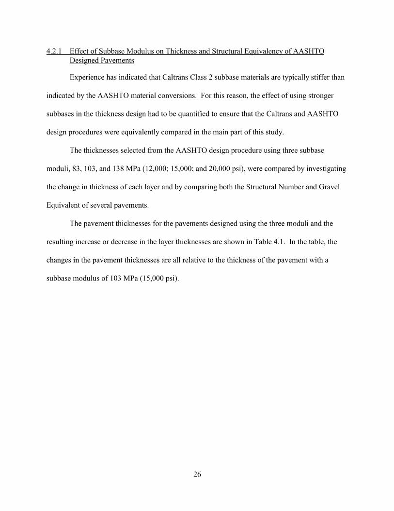
4.2.1 Effect of Subbase Modulus on Thickness and Structural Equivalency of AASHTODesigned Pavements

Experience has indicated that Caltrans Class 2 subbase materials are typically stiffer than

indicated by the AASHTO material conversions. For this reason, the effect of using stronger

subbases in the thickness design had to be quantified to ensure that the Caltrans and AASHTO

design procedures were equivalently compared in the main part of this study.

The thicknesses selected from the AASHTO design procedure using three subbase

moduli, 83, 103, and 138 MPa (12,000; 15,000; and 20,000 psi), were compared by investigating

the change in thickness of each layer and by comparing both the Structural Number and Gravel

Equivalent of several pavements.

The pavement thicknesses for the pavements designed using the three moduli and the

resulting increase or decrease in the layer thicknesses are shown in Table 4.1. In the table, the

changes in the pavement thicknesses are all relative to the thickness of the pavement with a

subbase modulus of 103 MPa (15,000 psi).

Table 4.1 Effect of aggregate subbase modulus on layer thickness and gravel equivalent (AASHTO procedure)Subbase Layer Thickness (mm) Change* in Layer Thickness (mm) Change* in

Traffic Index R-value

Modulus (MPa) AC AB ASB

Structural Number

Gravel Equivalent

Asphalt Concrete

Aggregate Base

Aggregate Subbase

Gravel Equivalent

7 5 83 80 152 240 3.03 1.70 - - 44 0.14103 80 152 196 3.03 1.56138 80 152 155 3.03 1.43 - - -41 -0.13

9 5 83 117 152 414 2.80 2.45 - - 75 0.25103 117 152 339 2.80 2.20138 117 152 265 2.76 1.96 - - -74 -0.24

11 5 83 155 196 501 5.39 3.06 - 44 39 0.29103 155 152 462 5.39 2.78138 155 152 366 5.39 2.46 - - -96 -0.31

13 5 83 210 226 562 6.54 3.63 - 73 23 0.34103 210 153 539 6.54 3.29138 195 152 466 6.54 2.98 -15 - -73 -0.31

15 5 83 255 251 623 7.60 4.12 - 80 26 0.37103 255 171 597 7.60 3.75138 240 152 533 7.64 3.40 -15 -19 -64 -0.34

* change relative to modulus = 103 MPa case; positive indicates increase, negative indicates decrease27

28

For the thinner pavements (TI = 7, 9) the effect of changing the subbase modulus is to

change only the thickness of the subbase. Typically this change is approximately 20 percent,

either a 20 percent increase for the decreased modulus or a 20 percent decrease for the increased

modulus.

As TI increases, and the base thickness exceeds the minimum (150 mm); the base

thickness also changes. For TIs of 13 and 15, the effect of reducing the subbase modulus is to

increase the base and subbase thicknesses by approximately 47 and 4 percent, respectively.

At a TI of 13 and a TI of 15, the asphalt concrete thickness decreases for the 138 MPa

(20,000 psi) subbase modulus. This decrease is due to the reduction of the base thickness to the

minimum, which necessitates adjustment of the asphalt concrete to obtain the required Structural

Number. In both of these cases, the subbase thickness is also reduced.

In summary, the effect of the assumed subbase modulus for the AASHTO method using

the three values of modulus included here (83, 103, and 138 MPa) was to change the thickness of

some or all of the pavement layers. The changes are most likely significant and large enough to

influence the mechanistic-empirical fatigue analysis. For the purpose of this report, it is

sufficient to state that if a large modulus is assumed (e.g., the 138 MPa (20,000 psi) modulus),

longer fatigue lives would be experienced. The modulus of 103 MPa (15,000 psi) was

considered reasonable to use in the further analysis because 1) a modulus of 83 MPa (12,000 psi)

is not representative of the Caltrans conditions, and 2) a modulus of 138 MPa (20,000 psi) is too

large relative to the recommended AASHTO conversions and procedure, and will therefore not

facilitate a reasonable comparison between the Caltrans and AASHTO design methods.

29

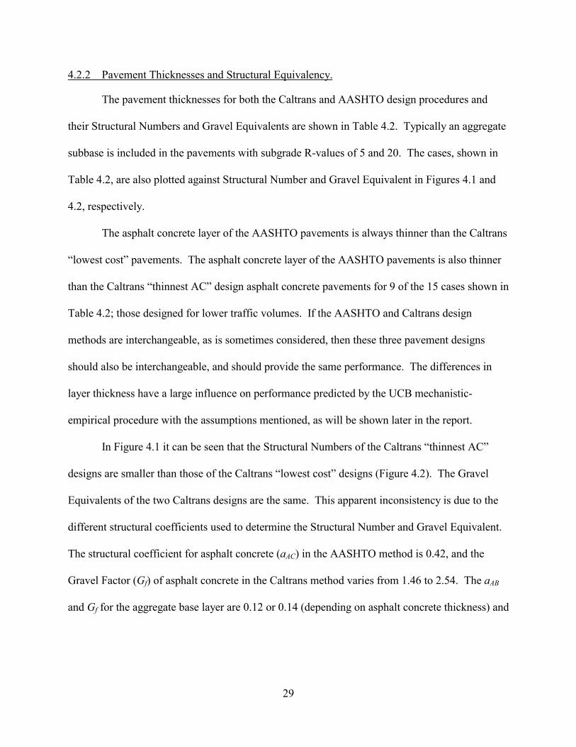
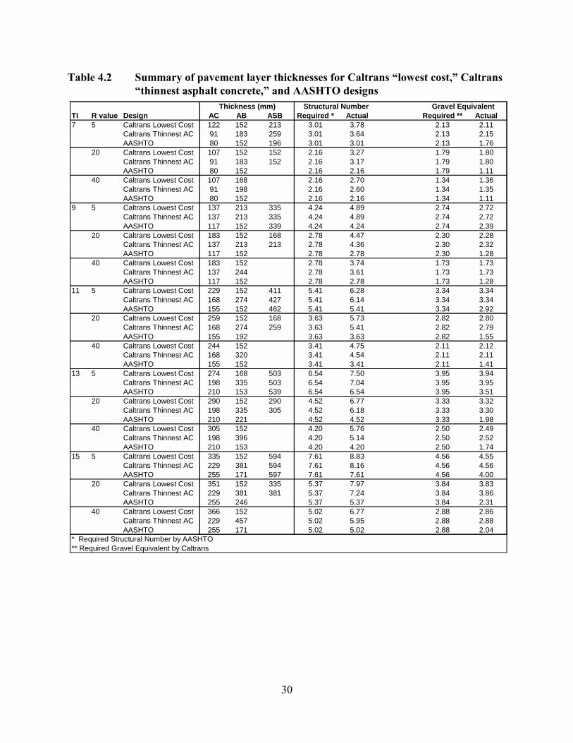
4.2.2 Pavement Thicknesses and Structural Equivalency.

The pavement thicknesses for both the Caltrans and AASHTO design procedures and

their Structural Numbers and Gravel Equivalents are shown in Table 4.2. Typically an aggregate

subbase is included in the pavements with subgrade R-values of 5 and 20. The cases, shown in

Table 4.2, are also plotted against Structural Number and Gravel Equivalent in Figures 4.1 and

4.2, respectively.

The asphalt concrete layer of the AASHTO pavements is always thinner than the Caltrans

“lowest cost” pavements. The asphalt concrete layer of the AASHTO pavements is also thinner

than the Caltrans “thinnest AC” design asphalt concrete pavements for 9 of the 15 cases shown in

Table 4.2; those designed for lower traffic volumes. If the AASHTO and Caltrans design

methods are interchangeable, as is sometimes considered, then these three pavement designs

should also be interchangeable, and should provide the same performance. The differences in

layer thickness have a large influence on performance predicted by the UCB mechanistic-

empirical procedure with the assumptions mentioned, as will be shown later in the report.

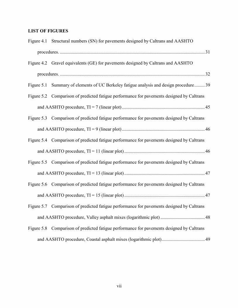
In Figure 4.1 it can be seen that the Structural Numbers of the Caltrans “thinnest AC”

designs are smaller than those of the Caltrans “lowest cost” designs (Figure 4.2). The Gravel

Equivalents of the two Caltrans designs are the same. This apparent inconsistency is due to the

different structural coefficients used to determine the Structural Number and Gravel Equivalent.

The structural coefficient for asphalt concrete (aAC) in the AASHTO method is 0.42, and the

Gravel Factor (Gf) of asphalt concrete in the Caltrans method varies from 1.46 to 2.54. The aAB

and Gf for the aggregate base layer are 0.12 or 0.14 (depending on asphalt concrete thickness) and

30

Table 4.2 Summary of pavement layer thicknesses for Caltrans “lowest cost,” Caltrans“thinnest asphalt concrete,” and AASHTO designs

Thickness (mm) Structural Number Gravel EquivalentTI R value Design AC AB ASB Required * Actual Required ** Actual7 5 Caltrans Lowest Cost 122 152 213 3.01 3.78 2.13 2.11

Caltrans Thinnest AC 91 183 259 3.01 3.64 2.13 2.15AASHTO 80 152 196 3.01 3.01 2.13 1.76

20 Caltrans Lowest Cost 107 152 152 2.16 3.27 1.79 1.80Caltrans Thinnest AC 91 183 152 2.16 3.17 1.79 1.80AASHTO 80 152 2.16 2.16 1.79 1.11

40 Caltrans Lowest Cost 107 168 2.16 2.70 1.34 1.36Caltrans Thinnest AC 91 198 2.16 2.60 1.34 1.35AASHTO 80 152 2.16 2.16 1.34 1.11

9 5 Caltrans Lowest Cost 137 213 335 4.24 4.89 2.74 2.72Caltrans Thinnest AC 137 213 335 4.24 4.89 2.74 2.72AASHTO 117 152 339 4.24 4.24 2.74 2.39












* Required Structural Number by AASHTO** Required Gravel Equivalent by Caltrans

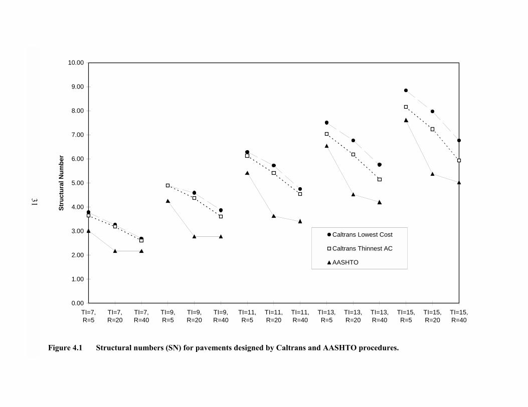
Figure 4.1 Structural numbers (SN) for pavements designed by Caltrans and AASHTO procedures.

0.00

1.00

2.00

3.00

4.00

5.00

6.00

7.00

8.00

9.00

10.00

TI=7,R=5

TI=7,R=20

TI=7,R=40

TI=9,R=5

TI=9,R=20

TI=9,R=40

TI=11,R=5

TI=11,R=20

TI=11,R=40

TI=13,R=5

TI=13,R=20

TI=13,R=40

TI=15,R=5

TI=15,R=20

TI=15,R=40

Stru

ctur

al N

umbe

r


Caltrans Thinnest AC

AASHTO

31

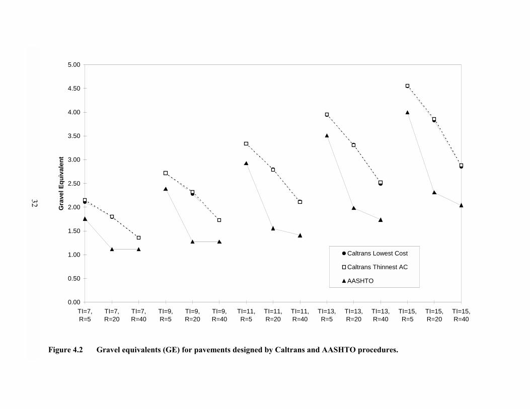
Figure 4.2 Gravel equivalents (GE) for pavements designed by Caltrans and AASHTO procedures.

0.00

0.50

1.00

1.50

2.00

2.50

3.00

3.50

4.00

4.50

5.00

TI=7,R=5

TI=7,R=20

TI=7,R=40

TI=9,R=5

TI=9,R=20

TI=9,R=40

TI=11,R=5

TI=11,R=20

TI=11,R=40

TI=13,R=5

TI=13,R=20

TI=13,R=40

TI=15,R=5

TI=15,R=20

TI=15,R=40

Gra

vel E

quiv

alen

t



AASHTO

32

33

1.1, respectively. The ratio of the asphalt concrete and aggregate base structural equivalencies is

approximately 3.23 for the AASHTO procedure and 1.33 to 2.24 for the Caltrans procedure.

These ratios show that the AASHTO method considers the asphalt concrete to add much more

structural capacity than the aggregate base, whereas the Caltrans procedure assigns less structural

capacity to the asphalt concrete layer.

The Gravel Equivalent is almost the same for the Caltrans “thinnest asphalt concrete” and

“lowest cost” designs, which implies that these pavements will provide the same performance.

As discussed in the next section, performance predictions indicate that these Caltrans “thinnest

AC” pavements have shorter fatigue lives than the Caltrans “lowest cost” pavements, which

suggests that the Gravel Factors may not be adequately proportioning the structural capacity of

the pavement to each layer and material type.

The Structural Number for the AASHTO pavements is considerably smaller than the

Caltrans pavements, indicating that the AASHTO designs are thinner and thus should withstand

less traffic. This is shown by the Gravel Equivalents of the pavements, as reported in Chapter 5.

As the TI increases, the difference in Structural Number between the Caltrans “lowest

cost” and Caltrans “thinnest AC” designs also increases. An increase in TI also causes an

increase in the Structural Number for the AASHTO pavements (Figures 4.1 and 4.2). For the

AASHTO pavements there appears to be a large difference between the Structural Number for

the subgrade R-values of 5 and 20. This suggests that the AASHTO design procedure may be

more sensitive to very low subgrade strengths than the Caltrans method.

34

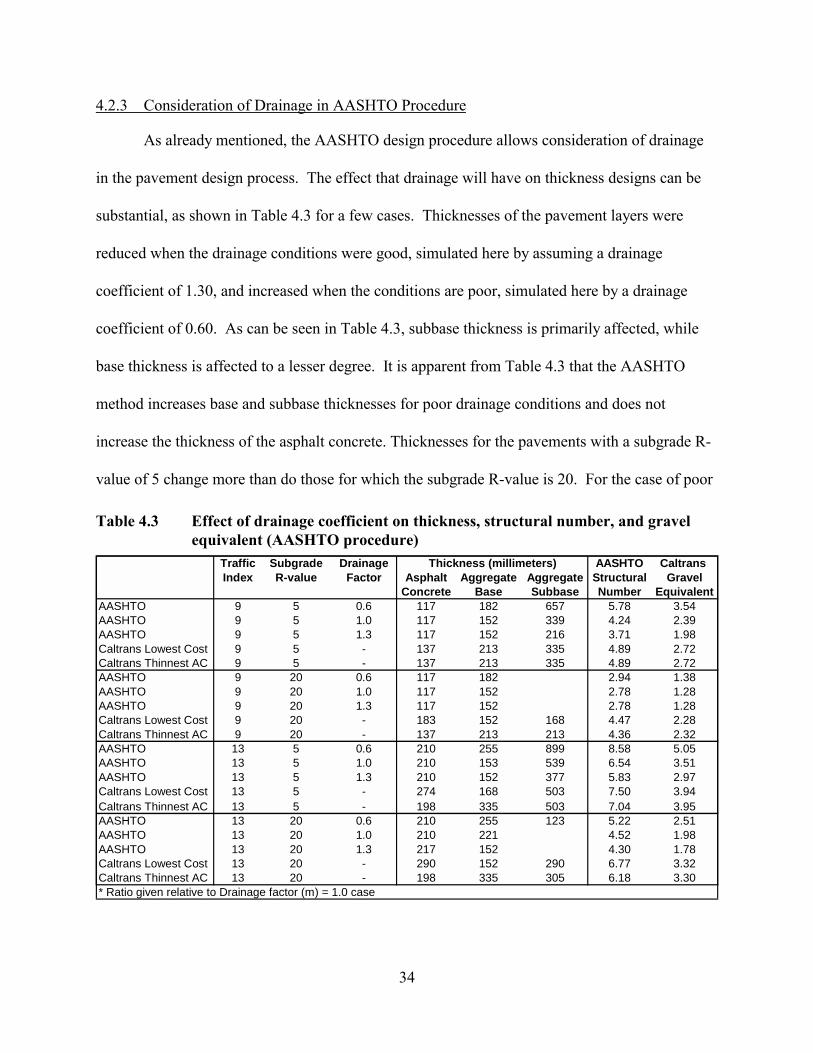
4.2.3 Consideration of Drainage in AASHTO Procedure

As already mentioned, the AASHTO design procedure allows consideration of drainage

in the pavement design process. The effect that drainage will have on thickness designs can be

substantial, as shown in Table 4.3 for a few cases. Thicknesses of the pavement layers were

reduced when the drainage conditions were good, simulated here by assuming a drainage

coefficient of 1.30, and increased when the conditions are poor, simulated here by a drainage

coefficient of 0.60. As can be seen in Table 4.3, subbase thickness is primarily affected, while

base thickness is affected to a lesser degree. It is apparent from Table 4.3 that the AASHTO

method increases base and subbase thicknesses for poor drainage conditions and does not

increase the thickness of the asphalt concrete. Thicknesses for the pavements with a subgrade R-

value of 5 change more than do those for which the subgrade R-value is 20. For the case of poor

Table 4.3 Effect of drainage coefficient on thickness, structural number, and gravelequivalent (AASHTO procedure)

Traffic Subgrade Drainage Thickness (millimeters) AASHTO Caltrans Index R-value Factor Asphalt Aggregate Aggregate Structural Gravel

Concrete Base Subbase Number EquivalentAASHTO 9 5 0.6 117 182 657 5.78 3.54AASHTO 9 5 1.0 117 152 339 4.24 2.39AASHTO 9 5 1.3 117 152 216 3.71 1.98Caltrans Lowest Cost 9 5 - 137 213 335 4.89 2.72Caltrans Thinnest AC 9 5 - 137 213 335 4.89 2.72AASHTO 9 20 0.6 117 182 2.94 1.38AASHTO 9 20 1.0 117 152 2.78 1.28AASHTO 9 20 1.3 117 152 2.78 1.28Caltrans Lowest Cost 9 20 - 183 152 168 4.47 2.28Caltrans Thinnest AC 9 20 - 137 213 213 4.36 2.32AASHTO 13 5 0.6 210 255 899 8.58 5.05AASHTO 13 5 1.0 210 153 539 6.54 3.51AASHTO 13 5 1.3 210 152 377 5.83 2.97Caltrans Lowest Cost 13 5 - 274 168 503 7.50 3.94Caltrans Thinnest AC 13 5 - 198 335 503 7.04 3.95AASHTO 13 20 0.6 210 255 123 5.22 2.51AASHTO 13 20 1.0 210 221 4.52 1.98AASHTO 13 20 1.3 217 152 4.30 1.78Caltrans Lowest Cost 13 20 - 290 152 290 6.77 3.32Caltrans Thinnest AC 13 20 - 198 335 305 6.18 3.30* Ratio given relative to Drainage factor (m) = 1.0 case

35

drainage, TI of 13, and R-value of 5, the AASHTO design results in more than 1.15 m (3.77 ft.)

of granular material.

For comparison, the pavement designs for the equivalent cases of the Caltrans “thinnest

asphalt concrete” and Caltrans “lowest cost” pavements are also shown in Table 4.3. For the

cases where the subgrade R-value is 5, the low drainage coefficient results in a pavement

structure that is thicker than both the Caltrans “thinnest asphalt concrete” and Caltrans “lowest

cost” pavements. This is not the case for the pavements with an R-value of 20. These

observations suggest that the Caltrans design method may be conservative with respect to

drainage and that if good drainage is present, the thickness design might be reduced, resulting in

cost savings.

While the current Caltrans design method does not explicitly consider drainage, an

alternative procedure is available to Caltrans in which such effects can be incorporated, i.e. with

the mechanistic-empirical fatigue analysis and design method utilized in Chapter 5. (15) In this

methodology, the effects of water content (or suction) on materials stiffness for use in pavement

analyses can be determined by laboratory tests or non-destructive measurements on existing

pavements. Such considerations may have a significant influence on pavement thickness, for

example, as illustrated in the current AASHTO method (Table 4.3). Thus, to improve the overall

performance of pavements in California and at the same time ensure that cost effective designs

are obtained, a more systematic approach should be adopted to consider the effects of water (and

drainage) on pavement response.

37

5.0 FATIGUE LIFE PREDICTIONS

5.1 UCB Design and Analysis Method

The fatigue analysis and design system used herein was originally developed as a part of

the Strategic Highway Research Program as a performance based procedure for designing asphalt

mixes to resist fatigue cracking. (16) Recently upgraded through the CAL/APT program, the

system considers not only fundamental mix properties but also the level of design traffic, the

temperature environment at the site, the pavement structural section, laboratory testing and

construction variabilities, and an acceptable level of risk. (2)

For the purposes of this study, the fatigue analysis and design system is used primarily to

estimate the number of ESALs that can be sustained for a selected design. The estimation is

based on the following equation:

(5.1)

in which ESALs = the number of equivalent, 80-kN (9,000-lb.) single axle loads that can be

sustained in situ before failure, N = the number of laboratory load repetitions to failure under the

anticipated in situ strain level, SF = a shift factor necessary to reconcile the difference between

fatigue in situ and that in the laboratory, TCF = a temperature conversion factor which converts

loading effects under the expected range of temperatures in the site-specific temperature

environment to those under the single temperature typically used in laboratory testing for

conventional asphalts (20°C), and M = a reliability multiplier based on the level acceptable risk

and variabilities associated with computing N and with estimating actual traffic loading. Figure

5.1 contains a flow diagram of ESALs determination embodied in this methodology.

MTCFSFNESALs•

•=

38

The estimate of N is based on laboratory testing, which measures the stiffness and fatigue

life of the asphalt mix, and on elastic multilayer analysis, which determines the initial critical

strain (εt) expected at the underside of the asphalt layer in situ under the standard 80-kN axle

load. It is simply fatigue life that would result from the repetitive application of the strain

expected in situ. The computer code, CIRCLY (17), was used for the elastic multilayer analyses

reported herein.

As mentioned previously, two asphalt concrete mixes were included in this study: one

containing a Coastal AR-4000 asphalt and the other a Valley AR-4000 asphalt. Both mixes use

the same aggregate and the same aggregate gradation. The relationships of fatigue versus tensile

strain are shown below for the Valley and Coastal mixes, respectively.

(Valley asphalt) (5.2a)

(Coastal asphalt) (5.2b)

where ln is the natural logarithm, N = laboratory fatigue life, AC and AV = asphalt and air-void

contents (percent), respectively, and εt = tensile strain at the bottom of the asphalt concrete layer.

Air-void and asphalt contents of 8 and 5 percent were assumed for both mixes.

tAVACN εln7176.316457.057520.0001.22ln −−+−=

tAVACN εln3606.419193.083988.0362.24ln −−+−=

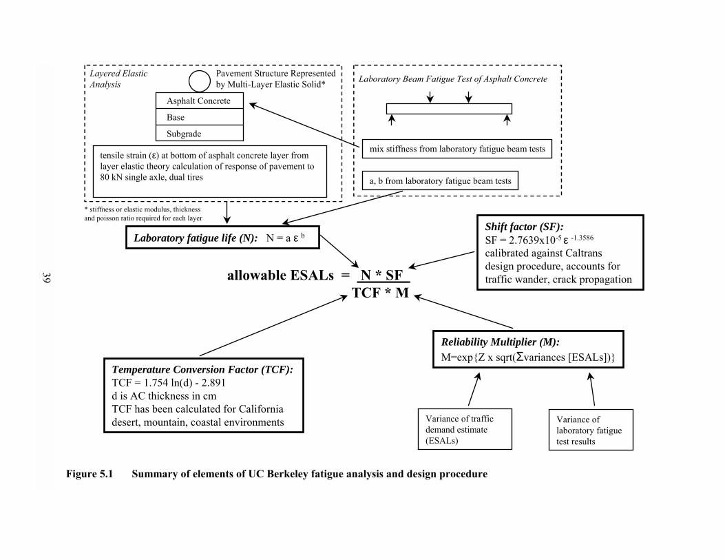
Figure 5.1 Summary of elements of UC Berkeley fatigue analysis and design procedure

allowable ESALs = N * SF TCF * M

Laboratory fatigue life (N): N = a ε bShift factor (SF):SF = 2.7639x10-5 ε=-1.3586

calibrated against Caltransdesign procedure, accounts fortraffic wander, crack propagation

Temperature Conversion Factor (TCF): TCF = 1.754 ln(d) - 2.891d is AC thickness in cmTCF has been calculated for Californiadesert, mountain, coastal environments

Reliability Multiplier (M):M=exp{Z x sqrt(Σvariances [ESALs])}

tensile strain (ε) at bottom of asphalt concrete layer fromlayer elastic theory calculation of response of pavement to80 kN single axle, dual tires a, b from laboratory fatigue beam tests

Variance of trafficdemand estimate(ESALs)

Variance oflaboratory fatiguetest results

mix stiffness from laboratory fatigue beam tests

Asphalt Concrete

Base

Subgrade

Pavement Structure Represented by Multi-Layer Elastic Solid* Laboratory Beam Fatigue Test of Asphalt ConcreteLayered Elastic

Analysis

* stiffness or elastic modulus, thicknessand poisson ratio required for each layer

39

40

The critical strain is also used in determining the shift factor1, SF, as follows:

(5.3)

The shift factor accounts for differences between laboratory and field conditions

including but not limited to traffic wander, crack propagation, and rest periods. The shift factor

relation is based on calibration of laboratory results against the Caltrans pavement thickness

design procedure. This shift factor was calibrated against pavements designed according to the

Caltrans procedure using the lowest initial cost, based on default costs, and only the mix

containing the Valley asphalt mix. (2) The shift factor may, therefore, be on the somewhat

conservative side.

The temperature conversion factor, TCF, has been previously determined for three

representative California environments including those in coastal, desert, and mountain regions,

an asphalt-aggregate mix containing a crushed gravel, and an AR-4000 asphalt refined from

California Coastal sources (the same asphalt included in this study). For this study, in-situ

performance simulations were based on the TCF for the coastal environment using the following

expression:

(5.4)

in which d = the asphalt concrete thickness in centimeters.

The reliability multiplier, M, is calculated as follows:

(5.5)

1 The shift factor and reliability multiplier used for this report is taken from (2). Later analyses that include theeffects of construction variance and use Monte Carlo simulations to determine the reliability multiplier (M) use thefollowing shift factor (11, 14): SF = 3.1833] 10-5 ε-1.3759

3586.15107639.2 −−•= tSF ε

891.2)ln(754.1 −= dTCF

)var(ln)var(ln ESALsNZeM +=

41

in which e = the base of natural logarithms, Z = a factor for the quantile of the standard normal

distribution depending solely on the design reliability, var(ln N) = the variance of the logarithm

of the laboratory fatigue life estimated at the in-situ strain level, and var(ln ESALs) = the variance

of the estimate of the logarithm of the design ESALs (i.e., the variance associated with

uncertainty in the traffic estimate). For this study, a 90-percent reliability level was selected for

which the Z value is 1.28. The var(ln N) was determined using the equation shown above and a

Monte Carlo simulation procedure. This procedure accounts for the inherent variability in

fatigue measurements, the nature of the laboratory testing program (principally the number of test

specimens and the strain levels), and the extent of extrapolation necessary for estimating fatigue

life at the design in-situ strain level. An assumed variance of the estimate of the design traffic

var(ln ESALs) of 0.3 has also been used in these calculations.

5.2 Fatigue Life Predictions

Fatigue life predictions presented in this section include a number of assumptions, the

reasonableness of which has been demonstrated in part by the Goal 1 CAL/APT test program.

Accordingly, they permit a uniform and quantitative means to compare the thickness designs

from the Caltrans and AASHTO methods.

The critical tensile strain at the bottom of the asphalt concrete layer for the pavement

thicknesses given in Table 4.2 under a 40-kN dual wheel load with center to center distance

between the wheels of 304 mm (12 inches), and a tire pressure of 690 kPa (100 psi) load was

calculated using elastic layer theory and the program CIRCLY. (17) This load is the “equivalent

single axle load” or “ESAL” to which all traffic loads are converted. Using the laboratory fatigue

life prediction equations, discussed in Section 5.1, and the assumed temperature conversion

42

factor, reliability factor, and shift factor, the predicted field fatigue life is determined. The values

used for the temperature conversion factor, the shift factor, and the reliability factor are shown in

Table 5.1. As already discussed, the temperature conversion factor is only dependent on the

thickness of the asphalt concrete layer. The shift factor, on the other hand, is dependent on the

tensile strain, which is a function of both the stiffness and thickness of the asphalt concrete layer.

The reliability factor is assigned and is therefore neither a function of thickness nor stiffness.

The results are shown in Table 5.2.

Figures 5.2 to 5.6 show plots of the fatigue life predictions versus subgrade R-value for

each Traffic Index. Figures 5.7 and 5.8 show the same data separated for each asphalt type on a

logarithmic plot. It can be seen in these figures that the pavements designed according to the

Caltrans “lowest cost” method typically give the longest fatigue life predictions for all the cases.

This result contrasts with the Gravel Equivalent results, which indicate that the Caltrans “thinnest

asphalt concrete” pavements have about the same Gravel Equivalents and therefore should

withstand traffic equally. The Caltrans “lowest cost” pavements have thicker asphalt concrete

layers than do the Caltrans “thinnest asphalt concrete” pavements, resulting in longer predicted

fatigue lives for the “lowest cost” designs. In the Caltrans “thinnest asphalt concrete” pavements,

the thinner asphalt concrete layer is compensated for by thicker base and subbase layers. The

longer predicted fatigue lives for the pavements with thicker asphalt concrete layers suggest that

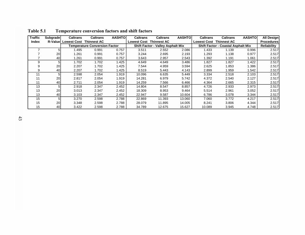
Table 5.1 Temperature conversion factors and shift factorsTraffic Subgrade Caltrans Caltrans AASHTO Caltrans Caltrans AASHTO Caltrans Caltrans AASHTO All DesignIndex R-Value Lowest Cost Thinnest AC Lowest Cost Thinnest AC Lowest Cost Thinnest AC Procedures

Temperature Conversion Factor Shift Factor - Valley Asphalt Mix Shift Factor - Coastal Asphalt Mix Reliability7 5 1.495 0.991 0.757 3.511 2.552 2.086 1.433 1.139 0.996 2.5177 20 1.261 0.991 0.757 3.244 2.695 2.193 1.293 1.138 0.977 2.5177 40 1.261 0.991 0.757 3.643 2.957 2.543 1.392 1.191 1.061 2.5179 5 1.702 1.702 1.425 4.649 4.649 3.486 1.827 1.827 1.422 2.5179 20 2.207 1.702 1.425 7.544 4.959 3.594 2.625 1.853 1.386 2.5179 40 2.207 1.702 1.425 8.519 5.443 4.143 2.899 1.959 1.542 2.517

11 5 2.598 2.054 1.919 10.096 6.635 5.449 3.334 2.518 2.103 2.51711 20 2.817 2.054 1.919 14.281 6.979 5.742 4.372 2.540 2.127 2.51711 40 2.711 2.054 1.919 14.259 7.566 6.466 4.364 2.665 2.315 2.51713 5 2.918 2.347 2.452 14.804 8.547 8.857 4.726 2.933 2.973 2.51713 20 3.013 2.347 2.452 18.309 8.953 9.464 5.514 2.961 3.052 2.51713 40 3.103 2.347 2.452 22.947 9.587 10.604 6.786 3.078 3.344 2.51715 5 3.270 2.598 2.788 22.869 11.393 13.060 7.060 3.772 4.217 2.51715 20 3.348 2.598 2.788 28.079 11.895 14.005 8.241 3.806 4.344 2.51715 40 3.422 2.598 2.788 34.789 12.675 15.627 10.089 3.945 4.748 2.517

43

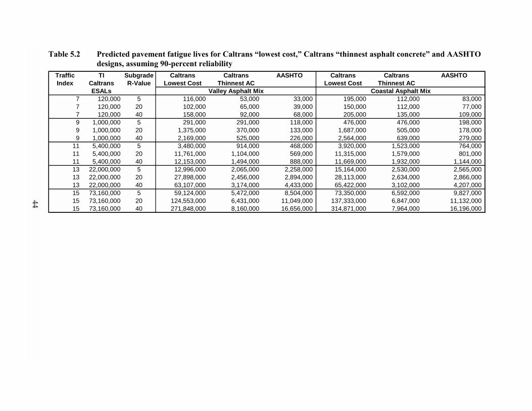
Table 5.2 Predicted pavement fatigue lives for Caltrans “lowest cost,” Caltrans “thinnest asphalt concrete” and AASHTOdesigns, assuming 90-percent reliability

Traffic TI Subgrade Caltrans Caltrans AASHTO Caltrans Caltrans AASHTOIndex Caltrans R-Value Lowest Cost Thinnest AC Lowest Cost Thinnest AC

ESALs Valley Asphalt Mix Coastal Asphalt Mix7 120,000 5 116,000 53,000 33,000 195,000 112,000 83,000 7 120,000 20 102,000 65,000 39,000 150,000 112,000 77,000 7 120,000 40 158,000 92,000 68,000 205,000 135,000 109,000 9 1,000,000 5 291,000 291,000 118,000 476,000 476,000 198,000 9 1,000,000 20 1,375,000 370,000 133,000 1,687,000 505,000 178,000 9 1,000,000 40 2,169,000 525,000 226,000 2,564,000 639,000 279,000

11 5,400,000 5 3,480,000 914,000 468,000 3,920,000 1,523,000 764,000 11 5,400,000 20 11,761,000 1,104,000 569,000 11,315,000 1,579,000 801,000 11 5,400,000 40 12,153,000 1,494,000 888,000 11,669,000 1,932,000 1,144,000 13 22,000,000 5 12,996,000 2,065,000 2,258,000 15,164,000 2,530,000 2,565,000 13 22,000,000 20 27,898,000 2,456,000 2,894,000 28,113,000 2,634,000 2,866,000 13 22,000,000 40 63,107,000 3,174,000 4,433,000 65,422,000 3,102,000 4,207,000 15 73,160,000 5 59,124,000 5,472,000 8,504,000 73,350,000 6,592,000 9,827,000 15 73,160,000 20 124,553,000 6,431,000 11,049,000 137,333,000 6,847,000 11,132,000 15 73,160,000 40 271,848,000 8,160,000 16,656,000 314,871,000 7,964,000 16,196,000

44

45

Figure 5.2 Comparison of predicted fatigue performance for pavements designed byCaltrans and AASHTO procedure, TI = 7 (linear plot)

-

50,000

100,000

150,000

200,000

250,000

5 20 40

Subgrade R-value

Fatig

ue li

fe (E

SALs

)

Traffic Index Caltrans Lowest Cost - ValleyCaltrans Lowest Cost - Coastal Caltrans Thinnest AC - ValleyCaltrans Thinnest AC - Coastal AASHTO - ValleyAASHTO - Coastal

46



-

500,000

1,000,000

1,500,000

2,000,000

2,500,000

3,000,000

5 20 40

Subgrade R-value

Fatig

ue li

fe (E

SALs

)

-

2,000,000

4,000,000

6,000,000

8,000,000

10,000,000

12,000,000

14,000,000

5 20 40Subgrade R-value

Fatig

ue li

fe (E

SALs

)

Traffic Index Caltrans Lowest Cost - Coastal

Caltrans Thinnest AC - Coastal AASHTO - Coastal

Caltrans Lowest Cost - Valley Caltrans Thinnest AC - Valley

AASHTO - Valley

47


-

50,000,000

100,000,000

150,000,000

200,000,000

250,000,000

300,000,000

350,000,000

5 20 40

Subgrade R-value

Fatig

ue li

fe (E

SALs

)

Traffic Index Caltrans Lowest Cost - Coastal

Caltrans Thinnest AC - Coastal AASHTO - Coastal

Caltrans Lowest Cost - Valley Caltrans Thinnest AC - Valley

AASHTO - Valley


-

10,000,000

20,000,000

30,000,000

40,000,000

50,000,000

60,000,000

70,000,000

5 20 40

Subgrade R-value

Fatig

ue li

fe (E

SALs

)

Figure 5.7 Comparison of predicted fatigue performance for pavements designed by Caltrans and AASHTO procedure,Valley asphalt mixes (logarithmic plot)

1.00E+04

1.00E+05

1.00E+06

1.00E+07

1.00E+08

1.00E+09

5 20 40 5 20 40 5 20 40 5 20 40 5 20 40

Subgrade R-Value

Fatig

ue li

fe (E

SALs

)



AASHTO

Traffic Index ESALs

Valley Asphalt Mix, 8 percent air-voids content

48

Figure 5.8 Comparison of predicted fatigue performance for pavements designed by Caltrans and AASHTO procedure,Coastal asphalt mixes (logarithmic plot)

1.00E+04

1.00E+05

1.00E+06

1.00E+07

1.00E+08

1.00E+09

5 20 40 5 20 40 5 20 40 5 20 40 5 20 40

Subgrade R-Value

Fatig

ue li

fe (E

SALs

)



AASHTO

Traffic Index ESALs

Coastal Asphalt Mix, 8 percent air-voids content

49

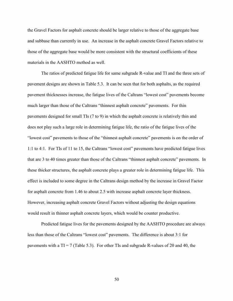
50

the Gravel Factors for asphalt concrete should be larger relative to those of the aggregate base

and subbase than currently in use. An increase in the asphalt concrete Gravel Factors relative to

those of the aggregate base would be more consistent with the structural coefficients of these

materials in the AASHTO method as well.

The ratios of predicted fatigue life for same subgrade R-value and TI and the three sets of

pavement designs are shown in Table 5.3. It can be seen that for both asphalts, as the required

pavement thicknesses increase, the fatigue lives of the Caltrans “lowest cost” pavements become

much larger than those of the Caltrans “thinnest asphalt concrete” pavements. For thin

pavements designed for small TIs (7 to 9) in which the asphalt concrete is relatively thin and

does not play such a large role in determining fatigue life, the ratio of the fatigue lives of the

“lowest cost” pavements to those of the “thinnest asphalt concrete” pavements is on the order of

1:1 to 4:1. For TIs of 11 to 15, the Caltrans “lowest cost” pavements have predicted fatigue lives

that are 3 to 40 times greater than those of the Caltrans “thinnest asphalt concrete” pavements. In

these thicker structures, the asphalt concrete plays a greater role in determining fatigue life. This

effect is included to some degree in the Caltrans design method by the increase in Gravel Factor

for asphalt concrete from 1.46 to about 2.5 with increase asphalt concrete layer thickness.

However, increasing asphalt concrete Gravel Factors without adjusting the design equations

would result in thinner asphalt concrete layers, which would be counter productive.

Predicted fatigue lives for the pavements designed by the AASHTO procedure are always

less than those of the Caltrans “lowest cost” pavements. The difference is about 3:1 for

pavements with a TI = 7 (Table 5.3). For other TIs and subgrade R-values of 20 and 40, the

Table 5.3 Ratios of predicted pavement fatigue lives for Coastal and Valley asphalt mixes.Traffic TI Subgrade Valley Asphalt Mix Coastal Asphalt MixIndex Caltrans R-Value CT lowest cost/ CT lowest cost/ CT thinnest AC/ CT lowest cost/ CT lowest cost/ CT thinnest AC/

ESALs CT thinnest AC AASHTO AASHTO CT thinnest AC AASHTO AASHTO7 120,000 5 2.2 3.5 1.6 1.7 2.3 1.37 120,000 20 1.6 2.6 1.7 1.3 1.9 1.57 120,000 40 1.7 2.3 1.4 1.5 1.9 1.29 1,000,000 5 1.0 2.5 2.5 1.0 2.4 2.49 1,000,000 20 3.7 10.3 2.8 3.3 9.5 2.89 1,000,000 40 4.1 9.6 2.3 4.0 9.2 2.3

11 5,400,000 5 3.8 7.4 2.0 2.6 5.1 2.011 5,400,000 20 10.7 20.7 1.9 7.2 14.1 2.011 5,400,000 40 8.1 13.7 1.7 6.0 10.2 1.713 22,000,000 5 6.3 5.8 0.9 6.0 5.9 1.013 22,000,000 20 11.4 9.6 0.8 10.7 9.8 0.913 22,000,000 40 19.9 14.2 0.7 21.1 15.6 0.715 73,160,000 5 10.8 7.0 0.6 11.1 7.5 0.715 73,160,000 20 19.4 11.3 0.6 20.1 12.3 0.615 73,160,000 40 33.3 16.3 0.5 39.5 19.4 0.551

52

Caltrans “lowest cost” pavements have fatigue lives about 10 to 20 times greater than those of

the AASHTO pavements. Lives of the Caltrans “lowest cost” pavements with a subgrade R-

value of 5 are only about 2 to 8 times longer than the AASHTO designs, indicating that these

designs are not as conservative when the two designs are compared for weaker subgrades.

Comparison of the Caltrans “thinnest asphalt concrete” pavements with the AASHTO

pavements indicates that the “thinnest asphalt concrete” pavements have fatigue lives 1.2 to 3

times longer than the AASHTO pavements for TIs of 7, 9, and 11. This difference is due to

thicker asphalt concrete and base layers in the Caltrans “thinnest asphalt concrete” pavements

than in the AASHTO pavements for these conditions. For TIs of 13 and 15, the Caltrans

“thinnest asphalt concrete” pavements have asphalt concrete layers 12 to 26 mm thinner and base

and subbase layers that are up to 2.5 times thicker than those of the AASHTO pavements (Table

4.2). For these designs, the predicted fatigue lives for the Caltrans “thinnest asphalt concrete”

pavements are at the most equal to and maybe as little as half those of the AASHTO pavements

(Table 5.3).

These results also imply that control of asphalt concrete thickness during construction is

important. This implication supports the study reported in Reference (5) for pay factor

associated with deviations in the thickness during construction.

For the comparisons shown in Table 5.3, the AASHTO pavements were designed based

on fair to good drainage conditions, which assumes the pavement structure is to be exposed to

water contents approaching saturation about 5 to 25 percent of the time. The Caltrans design

method utilizes results of the R-value test, in which the soil is tested in a near-saturated

53

condition.2 By considering various drainage conditions in the AASHTO procedure, it was shown

that the AASHTO procedure produces structures with thicker base and subbase layers when poor

drainage conditions are anticipated (Chapter 4). Assumption of poor drainage conditions in the

AASHTO procedures, and the resultant thicker structures, would result in less difference in

predicted pavement fatigue life between the Caltrans “thinnest asphalt concrete” and AASHTO

structures. Such results suggest that explicit consideration of drainage in the Caltrans procedure

may lead to considerably different pavement structures depending upon site-specific conditions

for expected rainfall, soil type, and potential drainage features included in the pavement.

Analytically-based methodology such as that utilized herein permits a direct consideration

of drainage effects on rehabilitation design if material properties are back-calculated from Falling

Weight Deflectometer (FWD) data collected at the wettest and driest times of the year.

Comparison of the predicted fatigue lives for the same pavement structures containing the

Valley and Coastal asphalts indicates that the mix with the Coastal asphalt provides better

performance for nearly every structure included in this study (Table 5.2, Figures 5.2 to 5.6).

Fatigue lives of these pavements are from 1.0 to 2.5 times greater than those for pavements

containing the mix with the Valley asphalt (Table 5.4). Calculations indicate that the Coastal

asphalt mix produces longer service lives as compared to the Valley asphalt mix for pavements

with Traffic Indices of 7, 9, and 11 and pavements with thinner asphalt concrete layers, which

include the Caltrans “thinnest asphalt concrete” and AASHTO designs. The Coastal asphalt mix

2 In the early work of Hveem, it was suggested that only about one third of the pavement subgrades becomesaturated. However, it was difficult to predict those which would develop these conditions. Hence, all are tested thisway to be on the conservative side. (16)

54

Table 5.4 Ratios of predicted pavement fatigue lives for Caltrans “lowest cost,”Caltrans “thinnest asphalt concrete” and AASHTO designs

also performs well relative to the Valley mix when the subgrade R-value is 5, as compared to

pavements with subgrade R-values of 20 and 40.

The Coastal asphalt mix has a lower stiffness than the Valley asphalt mix; lower mix

stiffnesses result in larger tensile strains for a given structure and load. The Coastal asphalt mix

also exhibits a larger number of load applications to failure for a given tensile strain than does

the Valley asphalt mix. It is therefore reasonable to expect that the Coastal asphalt mix will

perform particularly well relative to the Valley asphalt mix when the larger strains are expected,

e.g., for poor support conditions and for comparatively thin layers of asphalt concrete.

These results comparing the performance of the two mixes, in conjunction with other

results produced by the CAL/APT program illustrate the usefulness of the mechanistic-empirical

approach to integrate materials response characteristics and pavement design. (2, 5, 13, 15, 18)

Predicted Fatigue Life (ESALs) of Coastal Asphalt Mix Relative to Valley Asphalt Mix for Each Structure

Traffic TI SubgradeIndex Caltrans R-Value Caltrans Caltrans AASHTO

ESALs lowest cost thinnest AC7 120,000 5 1.7 2.1 2.57 120,000 20 1.5 1.7 2.07 120,000 40 1.3 1.5 1.69 1,000,000 5 1.6 1.6 1.79 1,000,000 20 1.2 1.4 1.39 1,000,000 40 1.2 1.2 1.2

11 5,400,000 5 1.1 1.7 1.611 5,400,000 20 1.0 1.4 1.411 5,400,000 40 1.0 1.3 1.313 22,000,000 5 1.2 1.2 1.113 22,000,000 20 1.0 1.1 1.013 22,000,000 40 1.0 1.0 0.915 73,160,000 5 1.2 1.2 1.215 73,160,000 20 1.1 1.1 1.015 73,160,000 40 1.2 1.0 1.0

55

The results also demonstrate that in the Caltrans and AASHTO design procedures, the

assumption that all asphalt concrete mixes have similar performance characteristics is likely not

valid. The results also demonstrate that both the pavement structure and associated layer

material characteristics determine fatigue performance and that designs associated with specified

reliability levels can be produced by the mechanistic analysis and design procedure described

herein (e.g., the 90 percent level illustrated in Figures 5.2 through 5.8 and Table 5.5).

It must be kept in mind that the shift factor included in the UCB procedure was calibrated

using the Caltrans “lowest cost” pavement design and the Valley asphalt mix with 8-percent air

voids. However, if that shift factor is assumed to be correct, the results would indicate that the

Caltrans “thinnest asphalt concrete” and the AASHTO pavement structures are generally not

adequate. In particular, the Caltrans “thinnest asphalt concrete” pavement structures for high

traffic levels (i.e., Traffic Indexes of 13 and 15) can only withstand about 10 to 40 percent of the

design ESALs with 90 percent reliability.

It is interesting to note that although the shift factor used herein was calibrated using the

Valley asphalt mix, the ratios of predicted fatigue life to design fatigue life appear to be similar

between the Valley and Coastal asphalt mixes. This similarity suggests that use of the Valley

asphalt mix for calibration does not produce unreasonable results for the other mix.

57

6.0 CONCLUSIONS AND RECOMMENDATIONS

6.1 Summary

This report has been prepared to compare the Caltrans and AASHTO pavement thickness

design procedures. The design comparisons included pavement structures subjected to a range in

traffic, as represented by Traffic Indexes of 7, 9, 11, 13, and 15, and a range in subgrade

strengths, as measured by subgrade R-values of 5, 20, and 40. Fatigue performance of the

pavement structures designed by the two procedures were predicted using the mechanistic-

empirical procedure developed as a part of the CAL/APT program. The various comparisons

presented provide the basis for recommendations for consideration by Caltrans relative to

pavement thickness design.

6.2 Conclusions

The following conclusions can be drawn from results presented in this report:

• The AASHTO and Caltrans pavement thickness design procedures do not produce the

same pavement structures for a given set of design inputs of subgrade strength, design

traffic, and pavement materials. Accordingly, these thickness design procedures

should not be used interchangeably. This conclusion is based on results that include

assumptions regarding comparable subgrade and pavement materials properties for a

given set of materials within the laboratory testing systems used for each design

procedure: R-value for the Caltrans procedure and resilient modulus (MR) for the

AASHTO procedure. Pavement structures produced by the two design procedures are

58

sensitive to the conversion from one type of laboratory test to the other, as was

demonstrated for the subbase layer in this report.

• Generally, pavement structures designed by the Caltrans procedure are thicker than

those designed by the AASHTO procedure.

• The relative contribution of asphalt concrete, granular base, and subbase materials to

a pavement structure’s load carrying capability is different for the two design

procedures. The ratio of the Gravel Factors of asphalt concrete to granular base is

between 1.33 to 2.54 in the Caltrans design procedure, and about 3.2 in the AASHTO

design procedure. Results presented in this report indicate that the structural

contribution of the asphalt concrete to fatigue cracking resistance for thicker asphalt

concrete layers is larger than is indicated by the Caltrans Gravel Factors.

• The predicted fatigue performance for the two Caltrans design options, “lowest cost”

(the layer thickness combination with the lowest construction cost in NEWCON90)

and “thinnest asphalt concrete layer allowed” is significantly different for most inputs

of Traffic Index and subgrade R-value. The “lowest cost” pavements, which have

thicker asphalt concrete layers, have predicted fatigue lives that are as much as 40

times longer at a Traffic Index of 15 than the pavements designed using the Caltrans

“thinnest asphalt concrete layer” design. Differences in predicted fatigue lives

between the Caltrans “lowest cost” pavements and the Caltrans “thinnest asphalt

concrete” pavements diminish for smaller Traffic Indices. It is therefore likely that

using the Caltrans procedure, alternative designs that are supposed to have similar

performance characteristics as measured by gravel equivalent (GE) will exhibit

59

different fatigue performance, with pavements using thinner asphalt concrete layers

not performing as well as pavements with thicker asphalt concrete layers.

• For Traffic Indices of 7, 9, and 11, the predicted fatigue lives of the Caltrans “thinnest

allowable asphalt concrete layer” pavements are about 1.5 to 2.8 times greater than

those of pavements designed using the AASHTO method with an assumed drainage

coefficient of 1.0. For more heavily trafficked pavements under the same drainage

condition, the AASHTO pavements typically have somewhat longer predicted fatigue

lives, approaching a factor of 2 at a Traffic Index of 15. Pavements designed by the

Caltrans methodology using the “lowest cost” option always have predicted fatigue

lives greater than those of pavements designed using the AASHTO method.

• Predicted pavement fatigue life is extremely sensitive to asphalt concrete thickness,

emphasizing an earlier recommendation that asphalt concrete thickness be included as

a pay factor variable in the Caltrans QC/QA procedures for asphalt concrete

construction. (5)

• Pavement drainage and lifecycle cost analyses are included explicitly in the AASHTO

procedure and currently available design software (DNPS86). While they are

required in the Caltrans design procedure, pavement drainage is not directly

accounted for and lifecycle cost analysis is not included in the currently available

design software. (9)

• While the thickness of asphalt concrete remains constant with changes in drainage

conditions in the AASHTO procedure, thicknesses of base and subbase layer can

change considerably depending upon expected drainage. The Caltrans procedure

60

assumes that pavement designs without special drainage priorities are adequate and

that their inclusion make Caltrans pavement designs conservative. However, no

quantitative analysis is performed to account for differences in the soils susceptibility

to water or rainfall for a particular location.

• Predicted pavement fatigue life is sensitive to different asphalt concrete mixes.

Results of fatigue estimates for pavements containing mixes using AR-4000 asphalt

binders from California Valley and California Coastal sources indicated that the

Coastal binder performed better in all of the structures analyzed. Differences in

predicted performance of pavements containing the two mixes depended on subgrade

support and the thickness of the asphalt concrete layer.

• Bearing in mind that the current laboratory-to-field shift factor included in the

University of California Berkeley fatigue analysis and design procedure was

calibrated against the Caltrans pavement design procedure “lowest cost” pavements,

and the Valley asphalt mix, the fatigue performance predictions suggest that Caltrans

“lowest cost” pavement designs are adequate at a 90-percent reliability level for all

Traffic Indices and subgrade R-values of 20 and 40. These results also suggest that

the Caltrans “lowest cost” pavement designs for a subgrade R-value of 5 may not be

adequate at this reliability level. Moreover, all Caltrans “thinnest allowable asphalt

concrete layer” designs are likely not adequate at the 90-percent reliability level. It

would also appear that AASHTO pavement designs may not be adequate at the 90-

percent reliability level. Substitution of the Coastal asphalt mix for the Valley asphalt

mix did not change these conclusions.

61

• Pavements designed for high volumes of truck traffic (i.e., Traffic Indexes of 13 and

15) using the Caltrans “thinnest allowable asphalt concrete layer” design appear to be

particularly vulnerable to premature fatigue cracking. Inclusion of thicker asphalt

concrete layers such as those used in the “lowest cost” pavements included in this

study appears to result in substantial improvement in predicted fatigue performance.

• The ability of the mechanistic-empirical pavement analysis and design procedure

described herein to quantitatively evaluate the effects of: 1) pavement structure,

including different layer thicknesses producing the same gravel equivalent; 2)

materials selection; and 3) subgrade strengths; has been demonstrated. Moreover, the

procedure directly relates the effects of pavement design, materials design, and

loading to a specific mode of pavement distress. Effects of drainage on pavement

performance can also be directly investigated provided stiffness characteristics of the

unbound materials are determined by laboratory tests for different levels of saturation.

6.3 Recommendations

Based on the information presented herein, the following recommendations are made:

1. Given that Caltrans and AASHTO design methods are not interchangeable, the

results of this report should be made available to agencies considering the use of

the AASHTO method for pavement design in California.

2. Lifecycle cost analysis should be included in any Caltrans design software. While

the Caltrans design manual requires lifecycle cost analysis for pavements designed

for larger Traffic Indices, a standard procedure for these analyses is not included

62

in the design procedure document (3), nor is it a part of the current design

software. (9)

3. Drainage considerations should be explicitly included in the Caltrans design

procedure. The current design procedure assumes that inclusion of drainage

features, such as asphalt treated permeable base (ATPB) and edge drains, will

improve the adequacy of designs. Results from the study of ATPB performed as a

part of the CAL/APT program indicate that this may not always be true. For

circumstances where drainage features do improve pavement performance, the

improvement should be quantified and included in lifecycle cost analyses. To

assist in this process, drainage coefficients could be developed for the existing

Caltrans procedures using the fatigue analysis and design procedure described in

this report. To accomplish this requires the conduct of laboratory tests to define

the effects of saturation on the stiffnesses of typical pavement materials and

methods to estimate the effects of drainage on saturation.

4. Gravel Factors for asphalt concrete should be re-evaluated. Results presented in

this report suggest that the structural value of asphalt concrete in reducing fatigue

damage is underestimated by the current Gravel Factors. The difference between

these factors and the apparent improvement in fatigue performance that comes

from thicker asphalt concrete layers is especially apparent for heavy-duty

pavements designed to carry large volumes of truck traffic.

5. Caltrans should move towards a mechanistic-empirical fatigue analysis and design

procedure for the design of asphalt concrete pavements. One framework that

might be followed is that utilized herein — it has the advantage of some

63

validation from the Goal 1 CAL/APT tests. Implementation can occur in stages,

and the following approach has a high probability of success.

a. Validate the procedure and its elements, such as the shift factor and

temperature conversion factor, by accelerated pavement testing. This first

step is already being carried out as part of Goal 1 of the CAL/APT

program.

b. Validate the procedure and its elements with long-term pavement

performance data. This step is more difficult than the first step, but is

necessary to obtain the confidence in the procedure needed for full-scale

implementation.

c. Use the procedure to “shadow” the current design procedure. This step

will permit comparison by designers and provide familiarity with the

procedure. It will also permit Caltrans to identify designs in the current

procedure that might not provide the desired performance because of

materials (for example the asphalt concrete mix), drainage, or other factors

not included in the current procedure.

d. Use the procedure to resolve questions and problems that cannot be

addressed by the current procedure, such as:

• the effects of water damage on materials (an example of this use is

included in Reference (3);

• the effects of trucks with different loading characteristics (weights,

axle configurations, tire pressures, etc.) that might be permitted on

64

California highways under the North American Free Trade Agreement

(NAFTA);

• the use of new materials, the properties of which can be determined in

the laboratory and included in analyses of the type presented in

Chapter 5 of this report; and

• the use of new types of asphalt pavement structures, for example, the

“rich-bottom” structure for fatigue resistance presented in another

report for Caltrans prepared by the University of California, Berkeley

(2).

e. Full-scale implementation.

65

7.0 REFERENCES

1. American Association of State Highway and Transportation Officials, AASHTO Guidefor Design of Pavement Structures, Washington, D.C., 1986.

2. Harvey, J., J. Deacon, B. Tsai, and C. Monismith, Fatigue Performance of AsphaltConcrete Mixes and its Relationship to Asphalt Concrete Pavement Performance inCalifornia, Report No. RTA-65W4845-2 for the California Department of Transportation,Institute of Transportation Studies, University of California, Berkeley, January, 1996.

3. California Department of Transportation, Highway Design Manual, Section 600,Sacramento, 1990.

4. Harvey, J., B. Tsai, F. Long, D. Hung, and C. Monismith, CAL/APT Program “AsphaltTreated Permeable Base (ATPB), Laboratory Testing, Performance, Predictions, andEvaluation of the Experience of Caltrans and Other Agencies,” Draft Report for theCalifornia Department of Transportation, Institute of Transportation Studies, Universityof California, Berkeley, June, 1997.

5. Deacon, J., C. Monismith, and J. Harvey, Pay Factors for Asphalt-Concrete Construction: Effect of Construction Quality on Agency Costs, Draft Technical Memorandum Preparedfor the California Department of Transportation, Institute of Transportation Studies,University of California, Berkeley, February, 1997.

6. Hveem, F. N., and R. M. Carmany, “The Factors Underlying the Rational Design ofPavements,” Proceedings, Highway Research Board, Vol. 28, 1948.

7. Sherman, G.B., “Recent Changes in the California Design Method for Structural Sectionsof Flexible Pavements,” Proceedings, First Annual Highway Conference, College ofPacific, Stockton, California, 1958.

8. Hveem, F. N., and G. B. Sherman, “Thickness of Flexible Pavements by the CaliforniaFormula Compared to AASHO Road Test Data,” Highway Research Record #13, 1963.

9. California Department of Transportation, NEWCON90 Computer Program, Based on1990 Version of Caltrans Highway Design Manual, Section 600.

10. Kallas, B., and J. Shook, San Diego County Experimental Base Project Final Report,Research Report 77-1 (RR-77-1), The Asphalt Institute, College Park, Maryland, 1977.

11. Harvey, J., and B. W. Tsai, “Effects of Asphalt Content and Air-Void Content on MixFatigue and Stiffness,” Transportation Research Record 1543, National ResearchCouncil, Washington D. C., 1996, pp. 38-45.

12. Harvey, J., and B. W. Tsai, “Long-Term Oven Aging Effects on Fatigue Life and InitialStiffness,” Accepted for publication by the Transportation Research Board, 1997.

13. Harvey, J., L. du Plessis, F. Long, J. Deacon, I. Guada, D. Hung, and C. Scheffy,CAL/APT Program: Test Results from Accelerated Pavement Test on PavementStructure Containing Asphalt Treated Permeable Base (ATPB) Section 500RF, ReportNo. RTA-65W4845-3 for the California Department of Transportation, Institute ofTransportation Studies, University of California, Berkeley, January, 1997.

14. ARE Inc., DNPS86 Computer Program Version 1, Prepared for AASHTO under NationalCooperative Highway Research Program Project 20-7/28, September, 1986.

15. Harvey, J., J. Deacon, A. Tayebali, R. Leahy, and C. Monismith, “A Reliability-BasedMix Design and Analysis System for Mitigating Fatigue Distress,” Accepted for

66

presentation and publication by the International Society for Asphalt Pavements, 8thInternational Conference, Seattle, 10B14 August, 1997.

16. Tayebali, A., J. Deacon, J. Coplantz, J. Harvey, F. Finn, and C. Monismith, FatigueResponse of Asphalt-Aggregate Mixes: Part I Test Method Selection; Part II ExtendedTest Program; Part III Mix Design and Analysis, Strategic Highway Research ProgramReport No. A-404, National Research Council, Washington, D.C., 1994.

17. Wardle, L., Program CIRCLY, User's Manual, Revision 1, Geomechanics ComputerProgram Number 2, Division of Applied Geomechanics, Commonwealth Scientific andIndustrial Research Organization, Melbourne, Australia, 1976.

18. Harvey, J., et al., CAL/APT Program: Test Results from Accelerated Pavement Test onPavement Structure Containing Untreated Aggregate Base Section 501RF, Draft Reportfor the California Department of Transportation, Institute of Transportation Studies,University of California, Berkeley, July, 1997.

cal/apt program comparison of caltrans and aashto pavement design … of ct and aashto.pdf ·...

Documents