Cadence Tutorial 1 The following Cadence CAD tools will be used in this tutorial:

• Virtuoso Schematic for schematic capture. • Analog Artist (Spectre) for simulation.

Computer Account Setup

Please revisit Unix Tutorial before doing this new tutorial.

If you use Exceed from a PC you need to take care of this extra issue. The Cadence software has an annoying screen/refresh problem when run on a PC via Exceed. You need to do the following in order to solve the problem: Under Xconfig -> Performance.

1. Enable Save Unders 2. Enable Change Maximum Backing Store to Always 3. Alter Default Backing Store to When Mapped 4. Alter Minimum Backing Store to When Mapped

You have to exit Exceed for the changes to take effect.

SETTING YOUR ENVIRONMENT UP FOR CADENCE AND ADDITIONAL TOOLS

In order to setup your environment to run Cadence applications you need to open an xterm window and type (EVERY TIME you login and in each window you want to run a Cadence tool)

. cdscdk2003

this script modifies your environment (sets PATH and exports variables). To see your current environment type the following at the prompt:

set

Running the Cadence tools

Now you should be able to run the Cadence tools. Never run Cadence from your root directory, it creates many extra files that will clutter your root. Instead please create a directory (e.g. cadence) and start Cadence there by typing:

mkdir cadence cd cadence icfb &

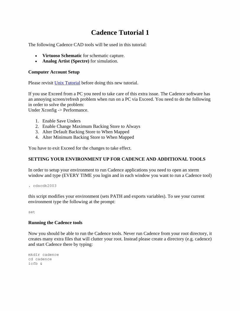
The command icfb & starts Cadence in the background and, after a couple of "update" messages that you can ignore for now (just click Continue) you should get a window with the icfb Command Interpreter Window (CIW) as below:

You will also get a "Cadence Update" window which you can read and then close or minimize. With the CIW you can launch other applications and you can also manage your files and libraries. NEVER use Unix commands (cp, mv) for moving Cadence design files as you may run into trouble later. For more information on the various Cadence tools I encourage you to read the corresponding user manuals. You can get to the manuals by pressing Help -> Cadence Documentation on any Cadence window (e.g. CIW). You can also open the on-line manuals by typing:

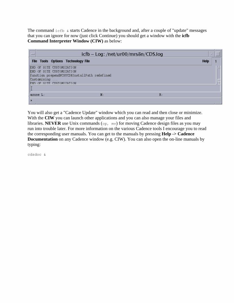
cdsdoc &

Spend some time browsing the manuals to understand what is available (a lot!). During the semester you will have to look for information in the on-line manuals to complement the (limited) info given by these tutorials.

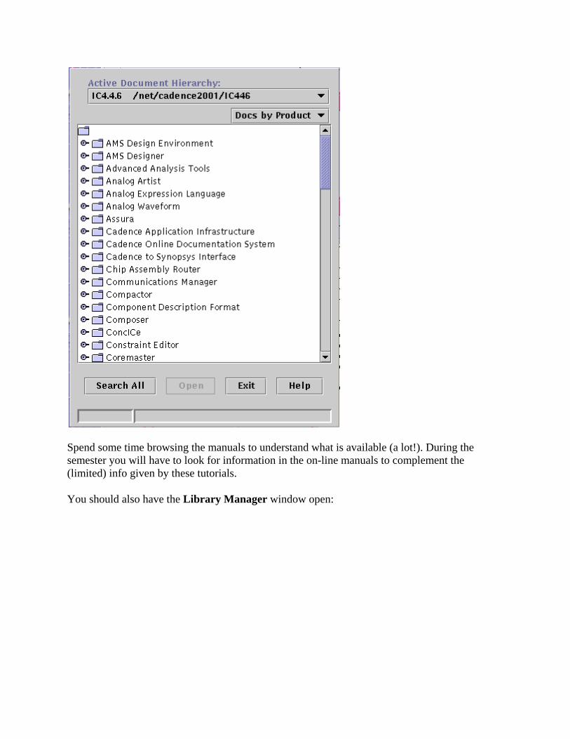
You should also have the Library Manager window open:

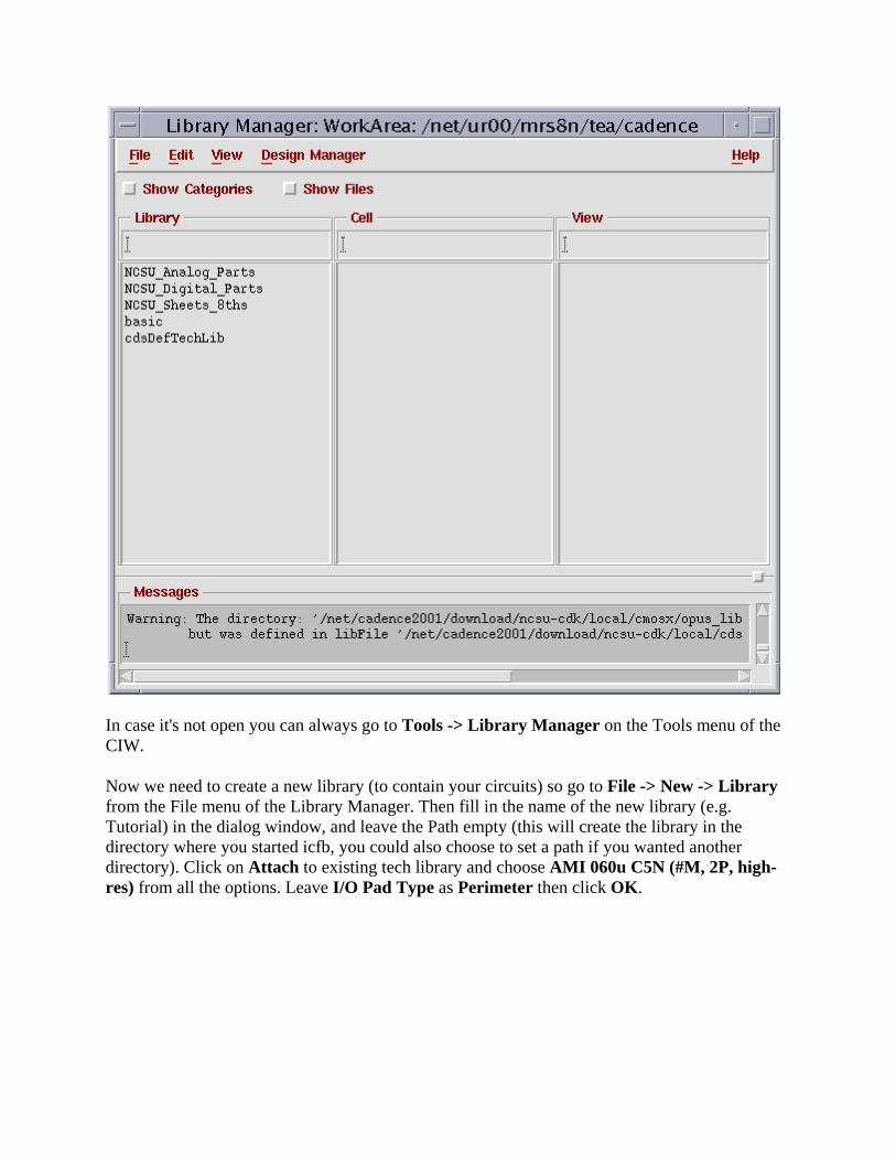
In case it's not open you can always go to Tools -> Library Manager on the Tools menu of the CIW.

Now we need to create a new library (to contain your circuits) so go to File -> New -> Library from the File menu of the Library Manager. Then fill in the name of the new library (e.g. Tutorial) in the dialog window, and leave the Path empty (this will create the library in the directory where you started icfb, you could also choose to set a path if you wanted another directory). Click on Attach to existing tech library and choose AMI 060u C5N (#M, 2P, high-res) from all the options. Leave I/O Pad Type as Perimeter then click OK.

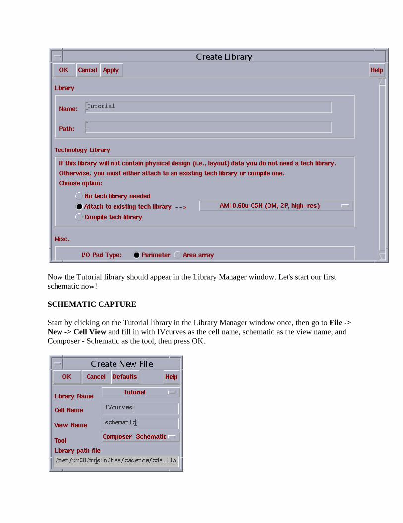
Now the Tutorial library should appear in the Library Manager window. Let's start our first schematic now!

SCHEMATIC CAPTURE

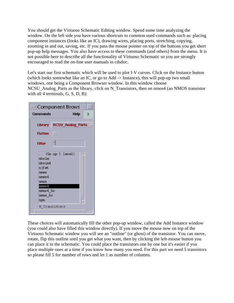
Start by clicking on the Tutorial library in the Library Manager window once, then go to File -> New -> Cell View and fill in with IVcurves as the cell name, schematic as the view name, and Composer - Schematic as the tool, then press OK.

You should get the Virtuoso Schematic Editing window. Spend some time analyzing the window. On the left side you have various shortcuts to common used commands such as: placing component instances (looks like an IC), drawing wires, placing ports, stretching, copying, zooming in and out, saving, etc. If you pass the mouse pointer on top of the buttons you get short pop-up help messages. You also have access to these commands (and others) from the menu. It is not possible here to describe all the functionality of Virtuoso Schematic so you are strongly encouraged to read the on-line user manuals in cdsdoc.

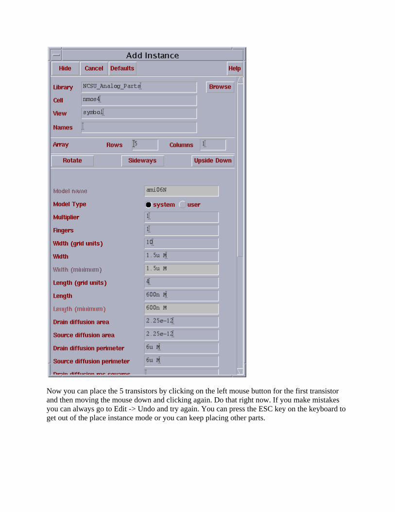
Let's start our first schematic which will be used to plot I-V curves. Click on the Instance button (which looks somewhat like an IC, or go to Add -> Instance), this will pop-up two small windows, one being a Component Browser window. In this window choose NCSU_Analog_Parts as the library, click on N_Transistors, then on nmos4 (an NMOS transistor with all 4 terminals, G, S, D, B):

These choices will automatically fill the other pop-up window, called the Add Instance window (you could also have filled this window directly). If you move the mouse now on top of the Virtuoso Schematic window you will see an "outline" (or ghost) of the transistor. You can move, rotate, flip this outline until you get what you want, then by clicking the left-mouse button you can place it in the schematic. You could place the transistors one by one but it's easier if you place multiple ones at a time if you know how many you need. For this part we need 5 transistors so please fill 5 for number of rows and let 1 as number of columns.

Now you can place the 5 transistors by clicking on the left mouse button for the first transistor and then moving the mouse down and clicking again. Do that right now. If you make mistakes you can always go to Edit -> Undo and try again. You can press the ESC key on the keyboard to get out of the place instance mode or you can keep placing other parts.

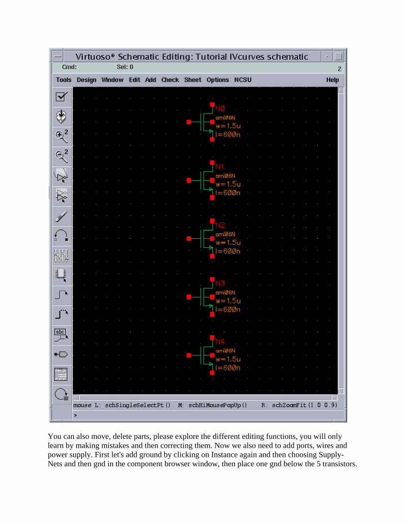
You can also move, delete parts, please explore the different editing functions, you will only learn by making mistakes and then correcting them. Now we also need to add ports, wires and power supply. First let's add ground by clicking on Instance again and then choosing Supply-Nets and then gnd in the component browser window, then place one gnd below the 5 transistors.

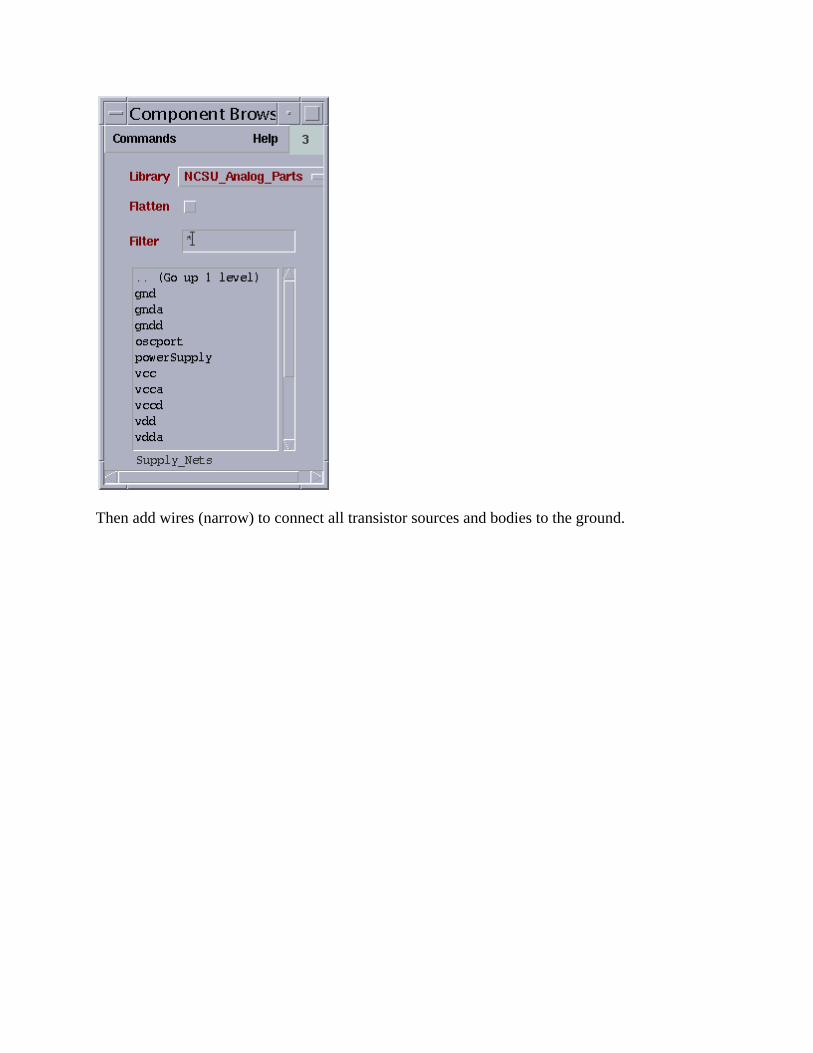
Then add wires (narrow) to connect all transistor sources and bodies to the ground.

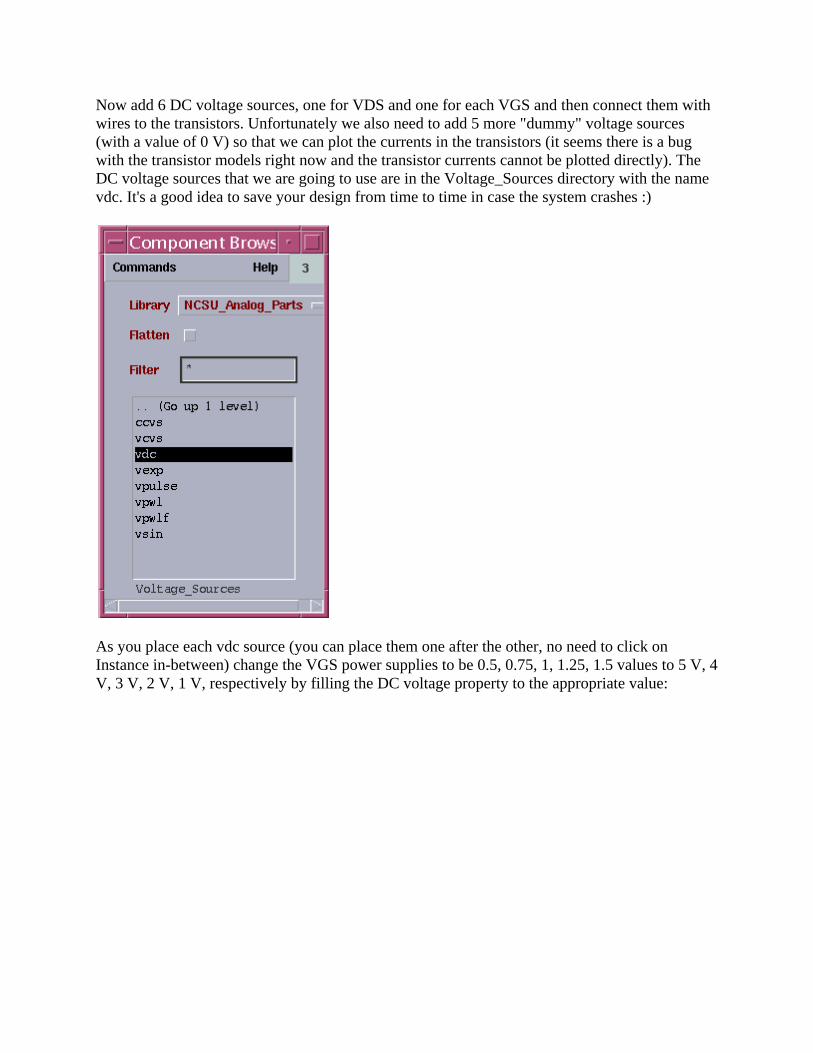
Now add 6 DC voltage sources, one for VDS and one for each VGS and then connect them with wires to the transistors. Unfortunately we also need to add 5 more "dummy" voltage sources (with a value of 0 V) so that we can plot the currents in the transistors (it seems there is a bug with the transistor models right now and the transistor currents cannot be plotted directly). The DC voltage sources that we are going to use are in the Voltage_Sources directory with the name vdc. It's a good idea to save your design from time to time in case the system crashes :)

As you place each vdc source (you can place them one after the other, no need to click on Instance in-between) change the VGS power supplies to be 0.5, 0.75, 1, 1.25, 1.5 values to 5 V, 4 V, 3 V, 2 V, 1 V, respectively by filling the DC voltage property to the appropriate value:

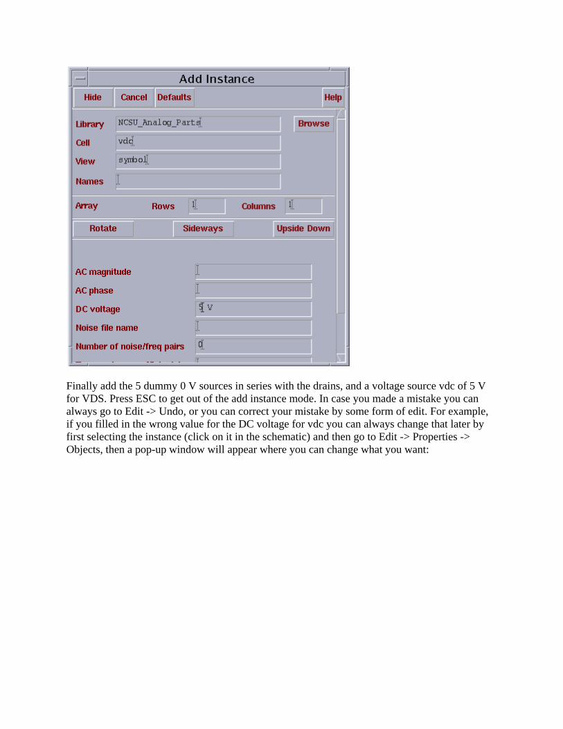
Finally add the 5 dummy 0 V sources in series with the drains, and a voltage source vdc of 5 V for VDS. Press ESC to get out of the add instance mode. In case you made a mistake you can always go to Edit -> Undo, or you can correct your mistake by some form of edit. For example, if you filled in the wrong value for the DC voltage for vdc you can always change that later by first selecting the instance (click on it in the schematic) and then go to Edit -> Properties -> Objects, then a pop-up window will appear where you can change what you want:

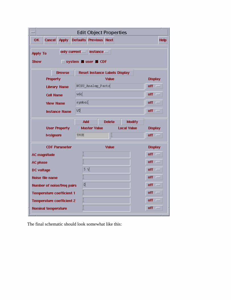
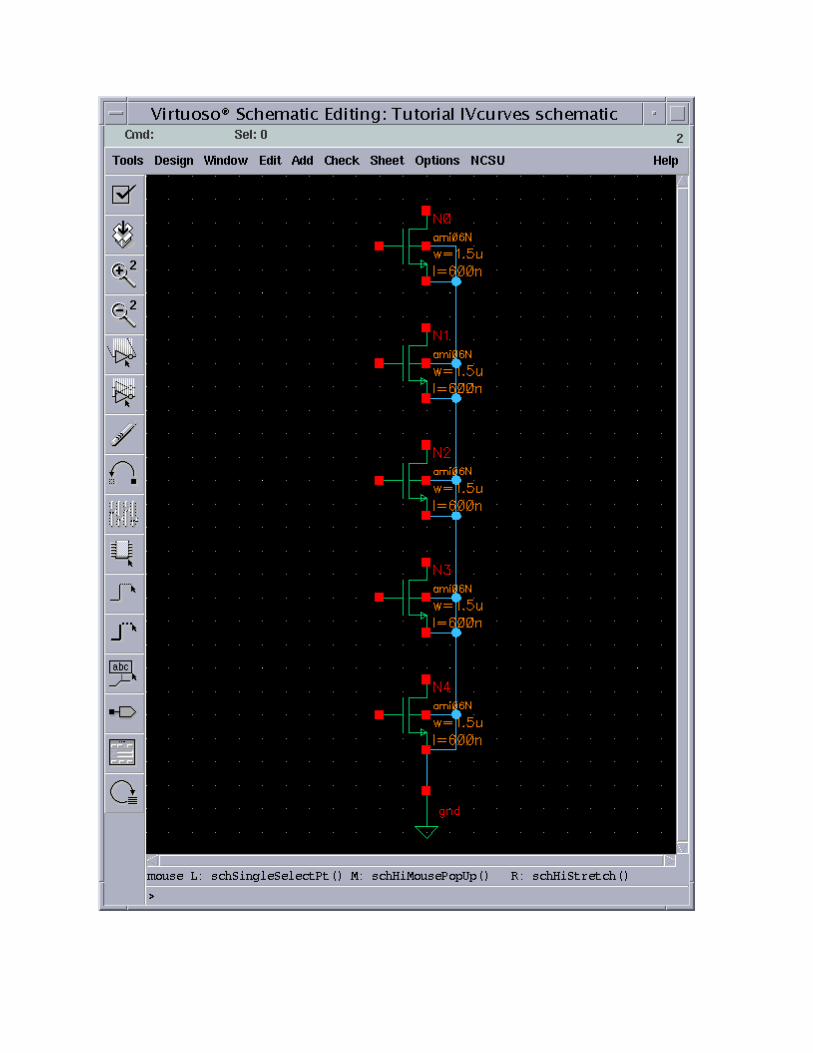
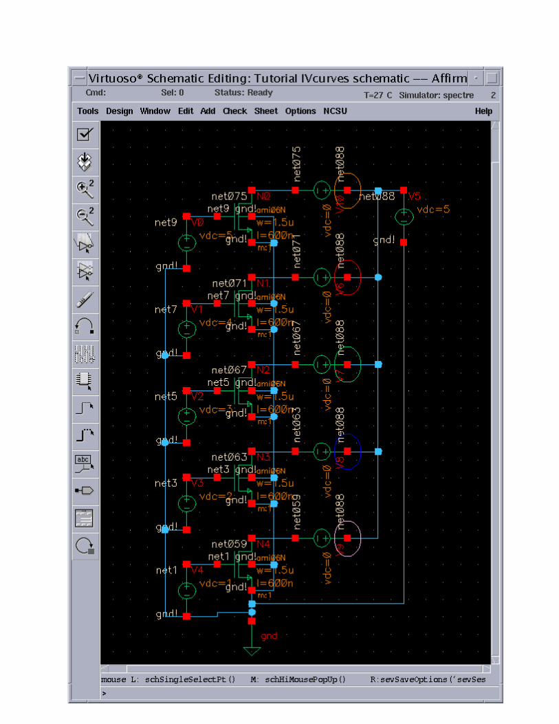
The final schematic should look somewhat like this:

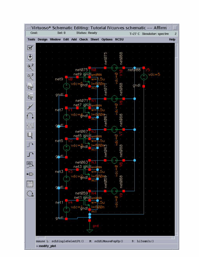
Now you need to Check and Save your design (either the top left button or Design -> Check and Save). Make sure you look at the CIW window and there are no errors or warnings, if there are any you have to go back and fix them!

Assuming there are no errors we are now ready to start simulation!

SIMULATION

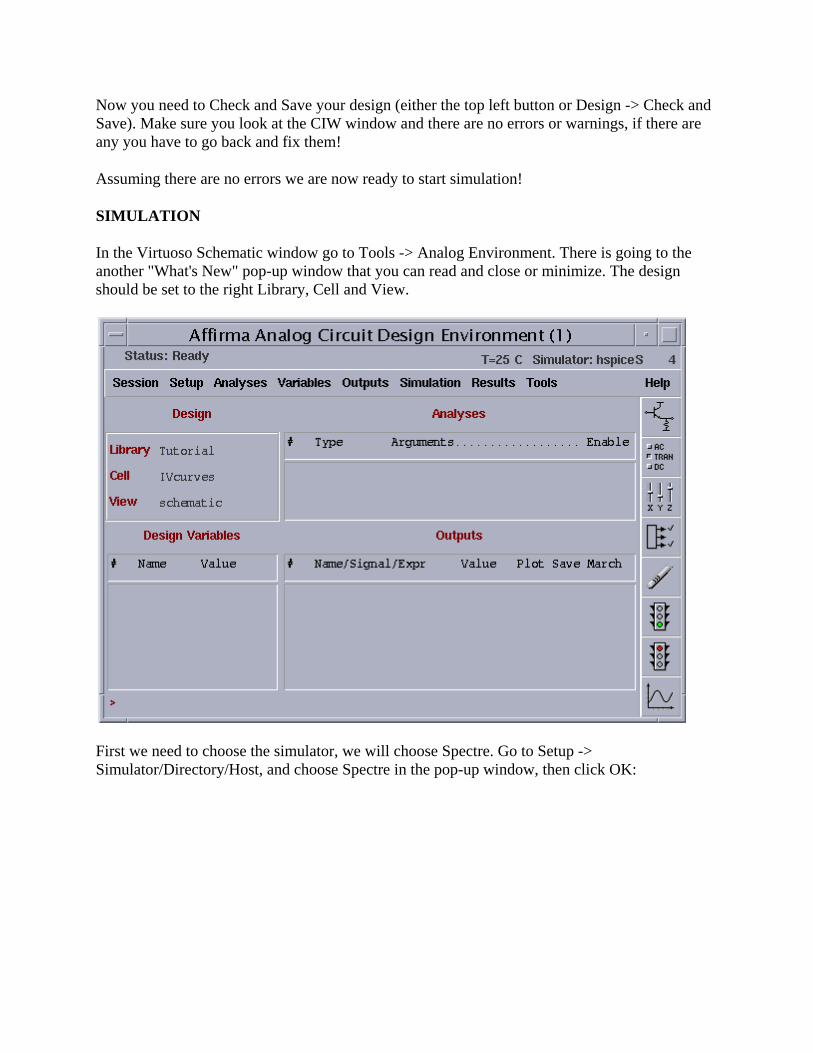
In the Virtuoso Schematic window go to Tools -> Analog Environment. There is going to the another "What's New" pop-up window that you can read and close or minimize. The design should be set to the right Library, Cell and View.

First we need to choose the simulator, we will choose Spectre. Go to Setup -> Simulator/Directory/Host, and choose Spectre in the pop-up window, then click OK:

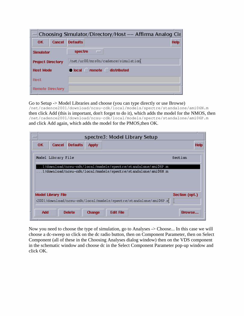
Go to Setup -> Model Libraries and choose (you can type directly or use Browse) /net/cadence2001/download/ncsu-cdk/local/models/spectre/standalone/ami06N.m then click Add (this is important, don't forget to do it), which adds the model for the NMOS, then /net/cadence2001/download/ncsu-cdk/local/models/spectre/standalone/ami06P.m and click Add again, which adds the model for the PMOS,then OK.

Now you need to choose the type of simulation, go to Analyses -> Choose... In this case we will choose a dc-sweep so click on the dc radio button, then on Component Parameter, then on Select Component (all of these in the Choosing Analyses dialog window) then on the VDS component in the schematic window and choose dc in the Select Component Parameter pop-up window and click OK.

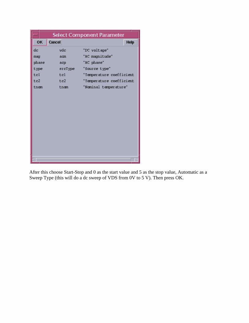
After this choose Start-Stop and 0 as the start value and 5 as the stop value, Automatic as a Sweep Type (this will do a dc sweep of VDS from 0V to 5 V). Then press OK.

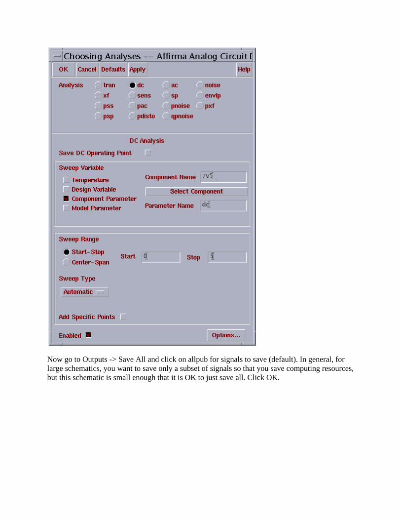
Now go to Outputs -> Save All and click on allpub for signals to save (default). In general, for large schematics, you want to save only a subset of signals so that you save computing resources, but this schematic is small enough that it is OK to just save all. Click OK.

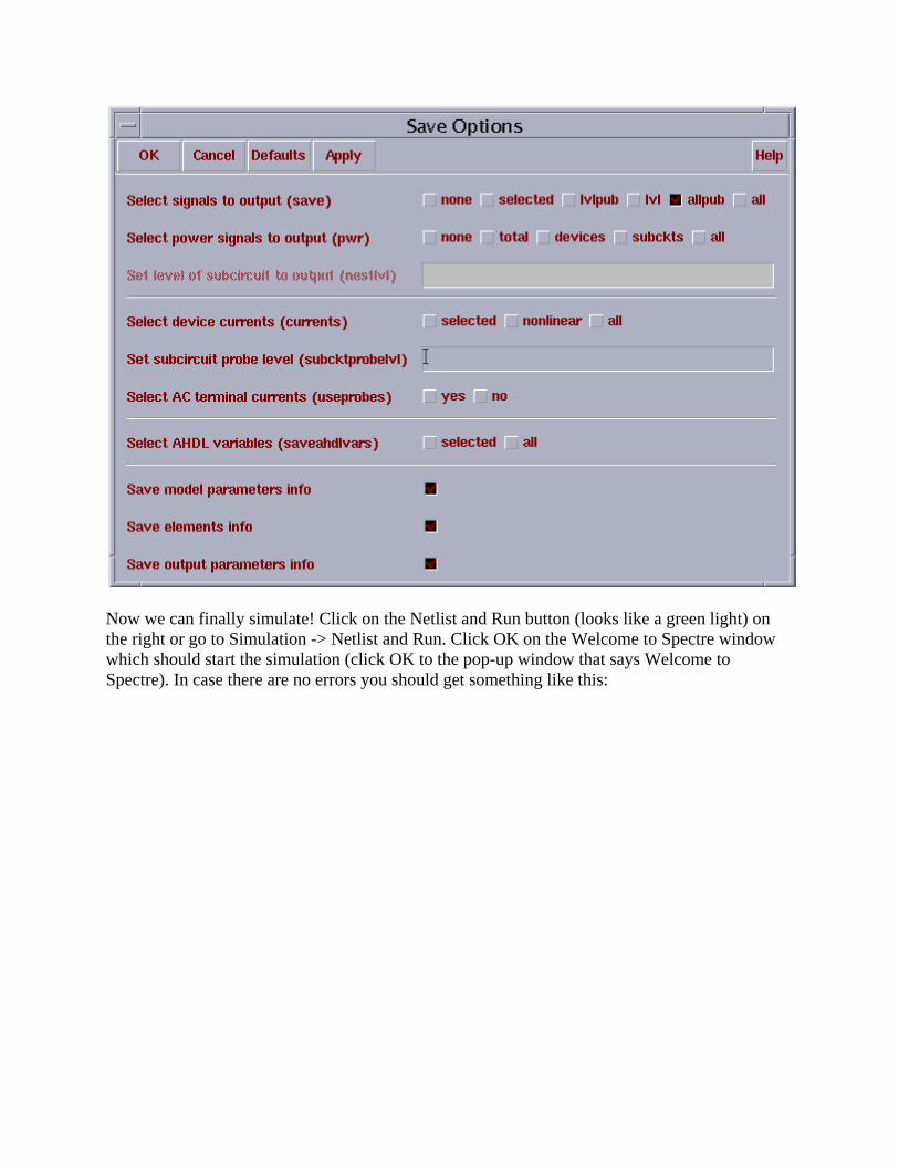
Now we can finally simulate! Click on the Netlist and Run button (looks like a green light) on the right or go to Simulation -> Netlist and Run. Click OK on the Welcome to Spectre window which should start the simulation (click OK to the pop-up window that says Welcome to Spectre). In case there are no errors you should get something like this:

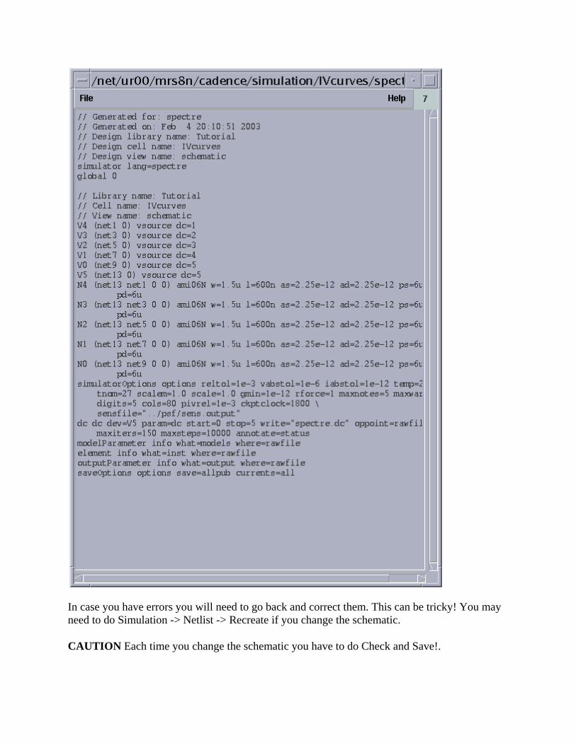
In case you have errors you will need to go back and correct them. This can be tricky! You may need to do Simulation -> Netlist -> Recreate if you change the schematic.

CAUTION Each time you change the schematic you have to do Check and Save!.

Assuming there are no errors you can now admire the simulation results. Go to Results -> Direct Plot -> DC which will pop-up your schematic window. Now you have to click on the signals you want to see. Since this is a dc-sweep we want to see the drain currents into the 5 transistors. In order to do this you have to click on the small red square at + terminal of each of the dummy power supplies in series with each drain. Make sure you click on the red square (the pin) which means current, versus any other part which means net, or voltage. Click on all 5 power supplies. If you are pressing right on the pins a circle should appear around each chosen pin.

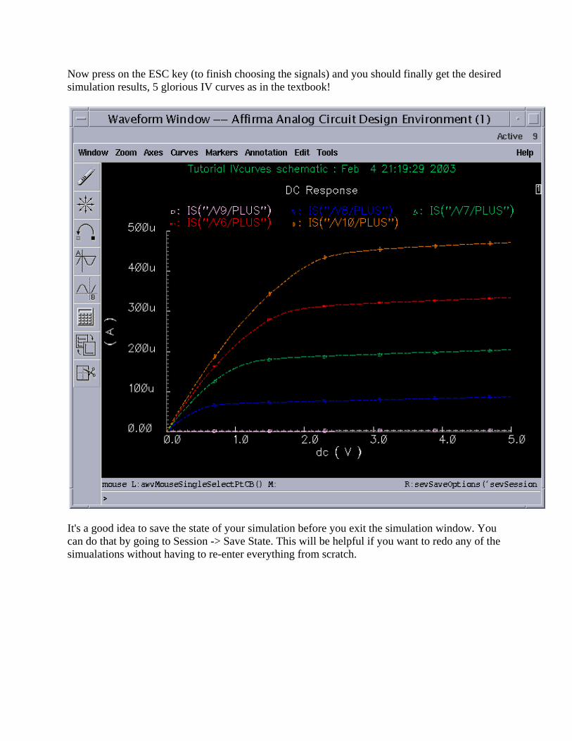
Now press on the ESC key (to finish choosing the signals) and you should finally get the desired simulation results, 5 glorious IV curves as in the textbook!

It's a good idea to save the state of your simulation before you exit the simulation window. You can do that by going to Session -> Save State. This will be helpful if you want to redo any of the simualations without having to re-enter everything from scratch.

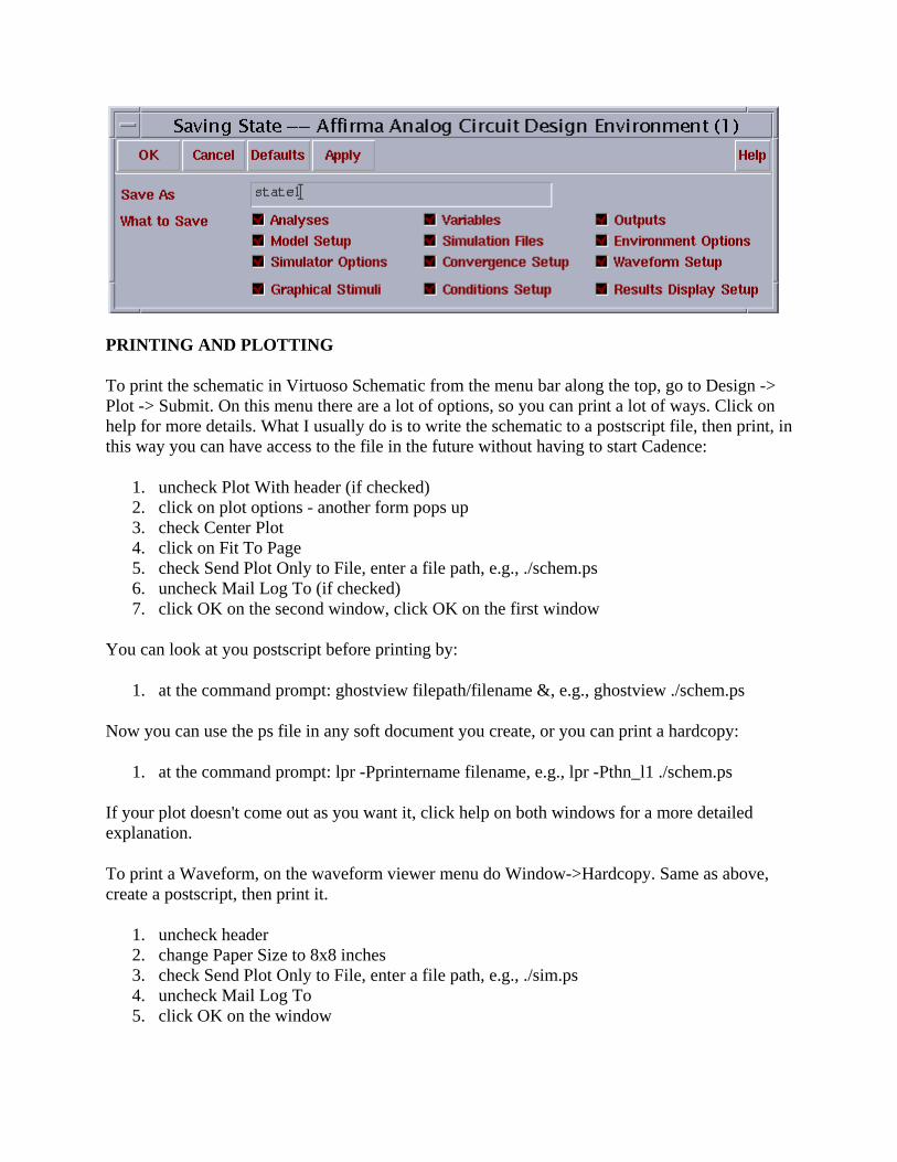
PRINTING AND PLOTTING

To print the schematic in Virtuoso Schematic from the menu bar along the top, go to Design -> Plot -> Submit. On this menu there are a lot of options, so you can print a lot of ways. Click on help for more details. What I usually do is to write the schematic to a postscript file, then print, in this way you can have access to the file in the future without having to start Cadence:

1. uncheck Plot With header (if checked) 2. click on plot options - another form pops up 3. check Center Plot 4. click on Fit To Page 5. check Send Plot Only to File, enter a file path, e.g., ./schem.ps 6. uncheck Mail Log To (if checked) 7. click OK on the second window, click OK on the first window

You can look at you postscript before printing by:

1. at the command prompt: ghostview filepath/filename &, e.g., ghostview ./schem.ps

Now you can use the ps file in any soft document you create, or you can print a hardcopy:

1. at the command prompt: lpr -Pprintername filename, e.g., lpr -Pthn_l1 ./schem.ps

If your plot doesn't come out as you want it, click help on both windows for a more detailed explanation.

To print a Waveform, on the waveform viewer menu do Window->Hardcopy. Same as above, create a postscript, then print it.

1. uncheck header 2. change Paper Size to 8x8 inches 3. check Send Plot Only to File, enter a file path, e.g., ./sim.ps 4. uncheck Mail Log To 5. click OK on the window

then do the same as you did for the schematic to print the hardcopy.

PARAMETRIC SIMULATION

After this long and tedious way to do things you will learn a faster way to do the same type of simulation as before. The idea is to understand that as an engineer you have many choices about how to achieve a desired result, and having more knowledge in general helps with finding a faster solution!

Until now we used multiple devices (5) in order to obtain the family of IV curves. We can achieve the same results by using a single transistor for which we change the voltage VGS. Close the Analog Environment and the IVcurves schematic and let's start another schematic, IVparam.

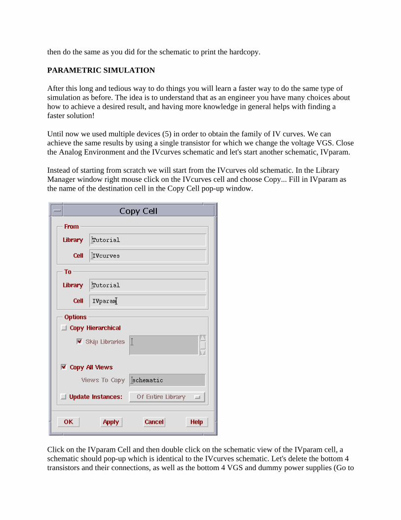
Instead of starting from scratch we will start from the IVcurves old schematic. In the Library Manager window right mouse click on the IVcurves cell and choose Copy... Fill in IVparam as the name of the destination cell in the Copy Cell pop-up window.

Click on the IVparam Cell and then double click on the schematic view of the IVparam cell, a schematic should pop-up which is identical to the IVcurves schematic. Let's delete the bottom 4 transistors and their connections, as well as the bottom 4 VGS and dummy power supplies (Go to

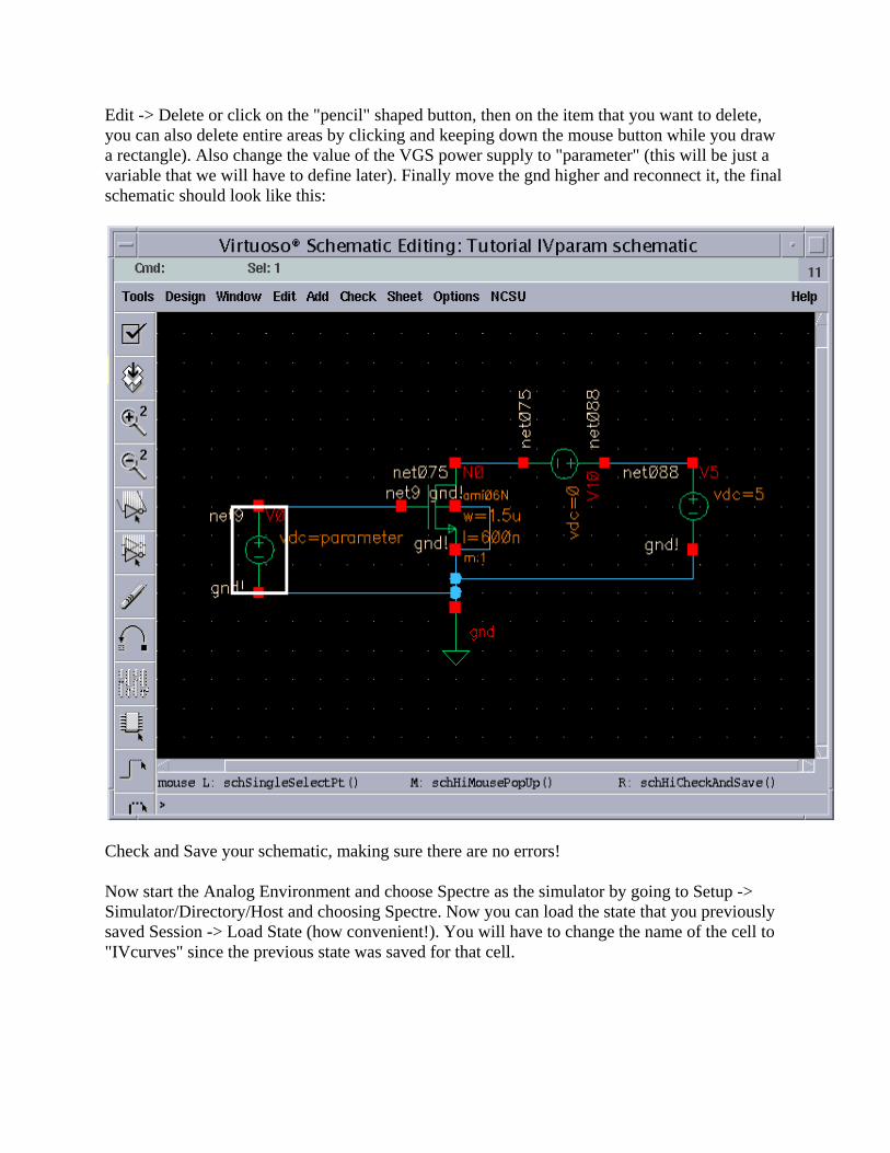
Edit -> Delete or click on the "pencil" shaped button, then on the item that you want to delete, you can also delete entire areas by clicking and keeping down the mouse button while you draw a rectangle). Also change the value of the VGS power supply to "parameter" (this will be just a variable that we will have to define later). Finally move the gnd higher and reconnect it, the final schematic should look like this:

Check and Save your schematic, making sure there are no errors!

Now start the Analog Environment and choose Spectre as the simulator by going to Setup -> Simulator/Directory/Host and choosing Spectre. Now you can load the state that you previously saved Session -> Load State (how convenient!). You will have to change the name of the cell to "IVcurves" since the previous state was saved for that cell.

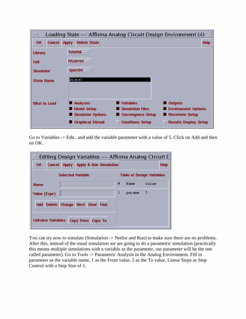
Go to Variables -> Edit.. and add the variable parameter with a value of 5. Click on Add and then on OK.

You can try now to simulate (Simulation -> Netlist and Run) to make sure there are no problems. After this, instead of the usual simulation we are going to do a parametric simulation (practically this means multiple simulations with a variable as the parameter, our parameter will be the one called parameter). Go to Tools -> Parametric Analysis in the Analog Environment. Fill in parameter as the variable name, 1 as the From value, 5 as the To value, Linear Steps as Step Control with a Step Size of 1.

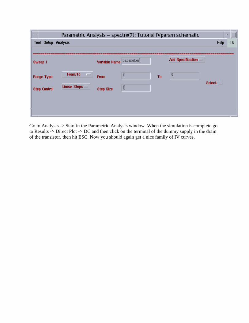
Go to Analysis -> Start in the Parametric Analysis window. When the simulation is complete go to Results -> Direct Plot -> DC and then click on the terminal of the dummy supply in the drain of the transistor, then hit ESC. Now you should again get a nice family of IV curves.

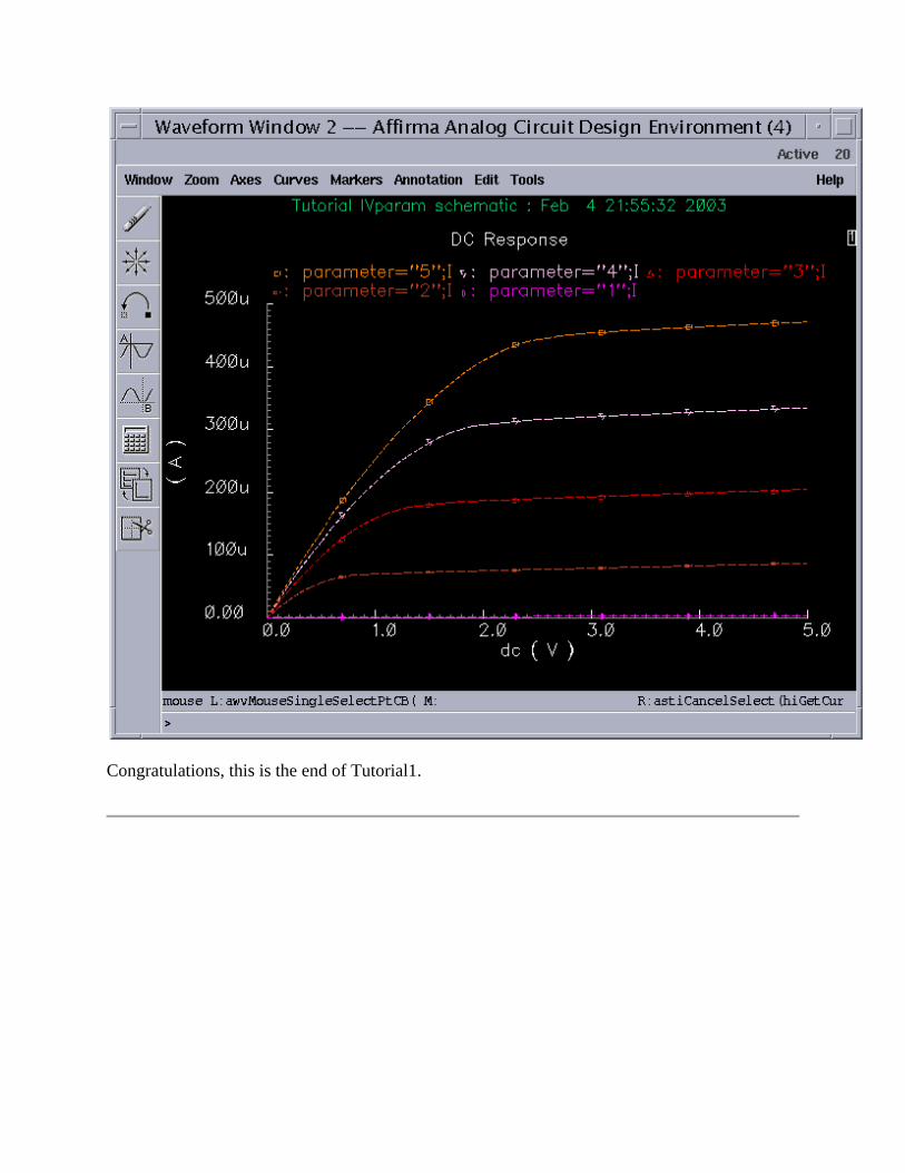
Congratulations, this is the end of Tutorial1.