C-POD: Validating cetacean detections 08/2013 not for printing – black graphs

send questions to Nick.Tregenza@chelonia.co.uk

To use acoustic data reliably you need to be able to carry out quality control assessments by visually checking the data. This requires some experience and this document is to help you get started. The main issue you will be trying to assess is the proportion of false positives. Taking porpoises first: False positives mainly come from:

1. Other cetaceans - dolphins classified as NBHF or NBHF as dolphins = BBTs. 2. Fine sand in suspension over the sea bed. These are ‘chance’ trains from a random source. 3. ADCPs - some acoustic Doppler current profilers make pulse trains at porpoise frequencies. 4. Boats sonars at porpoise frequencies. 5. WUTS - weak unknown train sources are known from a some sites, that seem to be high-nutrient sites. 6. Chain noise - ‘Chink spikes’ – quite rare, even when close to a chain. (another kind of ‘chance’ train) 7. Propellers, shrimp clicks etc. (also ‘chance’ trains) 8. Porpoise simulation tests!

The incidence of false positives from these sources is independent of the incidence of porpoise detections so the first question is: Q1: Do you have many porpoise detections?

• Yes, hundreds! The true positives will generally far outweigh these false positives and you can quickly view some samples and see how many train species identifications are uncertain or wrong. If the number of errors is much smaller than the number of true positives they will probably have no impact on the final statistical tests and you can proceed to export whatever you require, without editing the file to remove any errors.

• No: You will need to check all of them if the error rate is comparable to the true rate, and the true rate could be zero! But it won't take long - because there will be few trains you have to look at.

Q2: Can better performance be obtained from an encounter classifier? An encounter classifier ‘Hel1’ has been developed following an international workshop at the Hel Marine Station, Poland, using data gathered from the adjacent Puck Bay. This classifier can be applied, using CPOD.exe, after the KERNO classifier and takes a wider temporal ‘view’ of the data and greatly reduces false positives, at a cost of removing about 15% of the true positives. Encounter classifiers are essentially site specific. Puck Bay was a difficult site as a boat with a 130kHz sonar regularly used the Bay. In the areas of the Baltic Proper with no porpoises Hel1 gives much less than 1 false positive minute per year of continuous logging, despite logging huge numbers of sounds at porpoise frequencies. Where dolphins or WUTS are frequent Hel1 will not perform so well. An encounter classifier ‘GENENC’ was developed to reduce the level of false negatives in dolphin data from the Irish Sea and to give

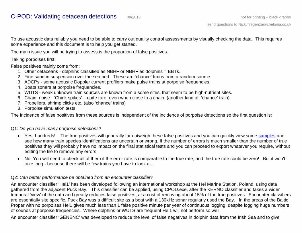
much better discrimination of Common Dolphins from Burmeister’s Porpoise in Peru. GENENC turns out to be useful in other locations as well, but you need to visually validate its performance. It often worth considering for dolphins if it produces a large increase in Detection Positive Minutes - DPM - compared the KERNO detector and you can find this quickly using the Analysis page. ‘GENENC2’ will be developed when we have enough examples of where it performs badly. Q3: How do I visually validate porpoise detections? Viewing the data Computer screens with very high horizontal resolution make this easier and more productive. A 3 screen display >5000pixels total wide is perfect (!), and CPOD.exe can use the whole width.

1. Open a file set so you can view the CP3 (train) and CP1(raw data) 2. Set time scale to 10ms 3. Set parameter to SPL 4. Set the filters to the classes you wish to validate, which are likely to be those shown here. If, for

this file processed through Hel1, you select ‘Harbour Porpoise’ then ‘all Q’ will also be checked as the normal setting.

5. If you are not using an encounter classifier click the ‘Seek’ label

which then becomes and allows you to see all the trains found, while being able to skip to the next Hi or Mod quality train.

You will now skip from one detection to the next, and the mouse wheel allows you to move backwards and forwards without 'seek' skipping the viewing point onwards to the next train. If you zoom in or out, using the down or up arrows, and want to get back to the point you were viewing in high resolution just click CTRL Z until your high resolution screen re-appears.

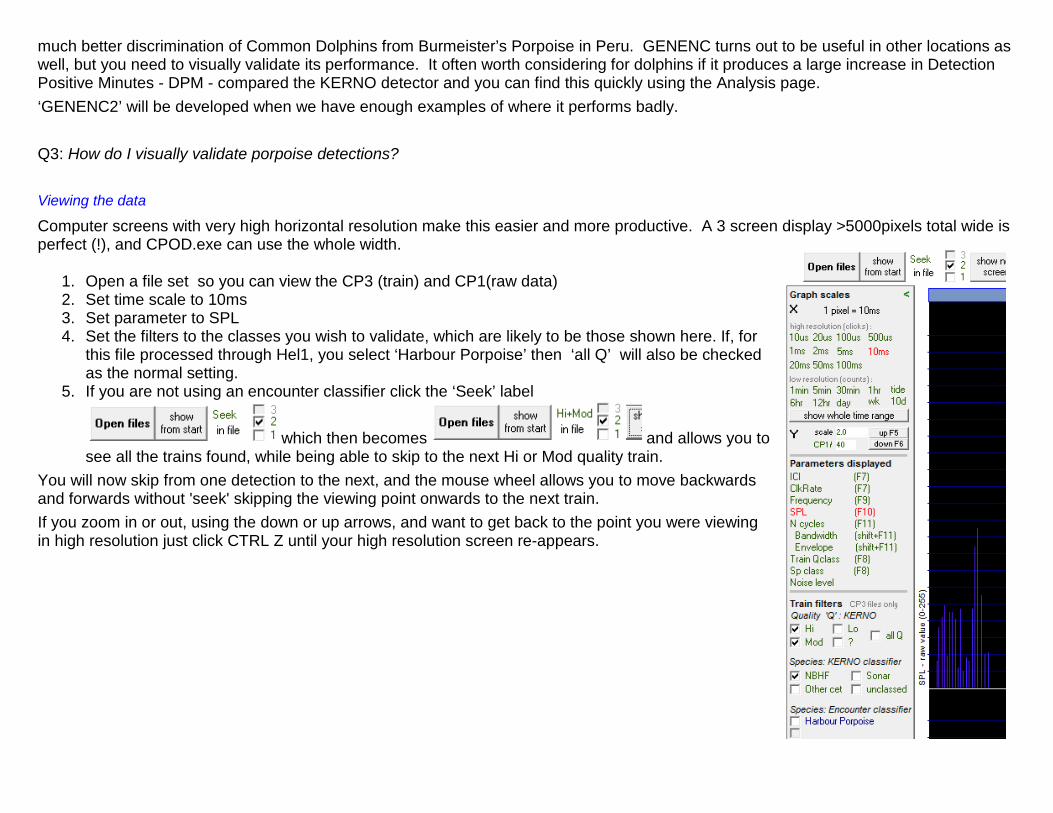
Chance train or real train?

The first question to resolve is whether the train comes from a train source or might be a chance train. Train Quality values represent how unlike chance trains they are. The features that favour a train coming from a train source are coherence, a quiet background and a temporal association with other trains or train fragments. A chance train (? Quality) A coherent train from a train source – a porpoise.

Coherence: Similar characteristics are seen in successive clicks where they all come from the same source. Look for these features to test whether a train is really a train or just a chance sequence: • SPL (sound pressure level) is the most useful, with true trains having a more or less even profile while chance trains have a ragged

profile. • Duration of clicks (number of cycles) – this usually shows a less smooth profile than SPL but is of value. • Multipath cluster size and shape. Multipath cluster are the bunches of multipath replicates that may follow a click, especially in shallow

water. They are evidence that the source was loud and if the cluster has a similar shape after successive clicks it shows that it has propagated along a similar pathway.

• Frequency – useful, but caution is needed. In some places tonal sediment noise may be within quite a narrow band so that chance trains may be found that have a narrow frequency range. Porpoise trains are mostly around 127 – 140khz. Dolphin trains are surprisingly variable and their multipath clusters show a wide spread across frequencies.

A quiet background : When there are only a few non-train clicks before, during and after a train it is likely to come from a train source. Actually if there are few clicks coming in the chance of a purely chance occurrence of a train can be extremely low. This probability can be formalised and this probability model of a train is key component of the train detector.

Temporal association with other trains: Cetaceans and boat sonars mostly produce trains more or less continuously, and their detected trains are nearly always accompanied in the data record by other trains, and fragments of trains, from the same source, that are not recognised by the classifier. The term 'train' is used here to mean the train received. The train produced by the source, whether boat or animal, will almost always be longer. Cetaceans sweep their environment with their sonar beam so a C-POD rarely gets a single train from a passing animal. When animals are in groups several individuals may score hits on the logger at different times during an encounter. Boat sonars are received mostly as echoes over a few minutes as the boat goes past. At the limit of detection range it is possible to get a single train from either a boat or a cetacean, but it is more difficult to be confident about its classification.

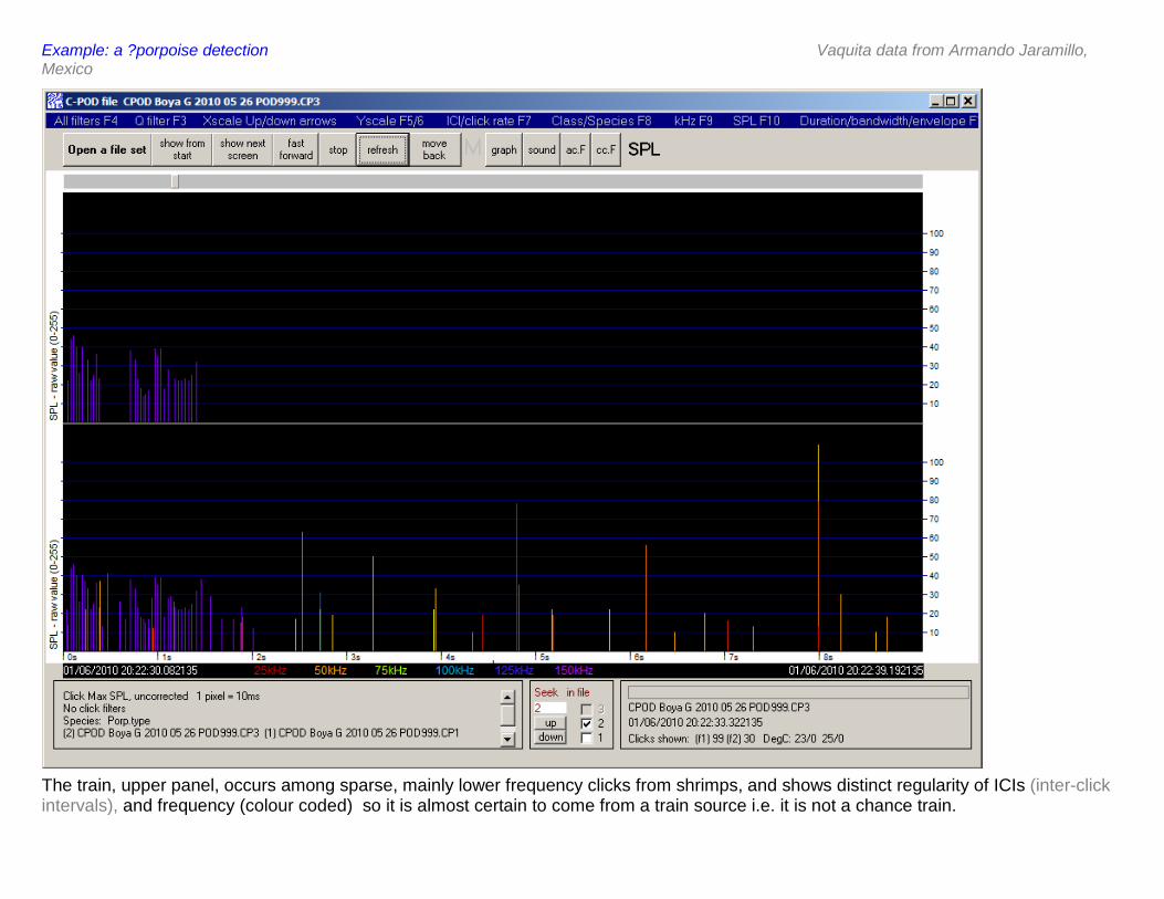
Example: a ?porpoise detection Vaquita data from Armando Jaramillo, Mexico

The train, upper panel, occurs among sparse, mainly lower frequency clicks from shrimps, and shows distinct regularity of ICIs (inter-click intervals), and frequency (colour coded) so it is almost certain to come from a train source i.e. it is not a chance train.

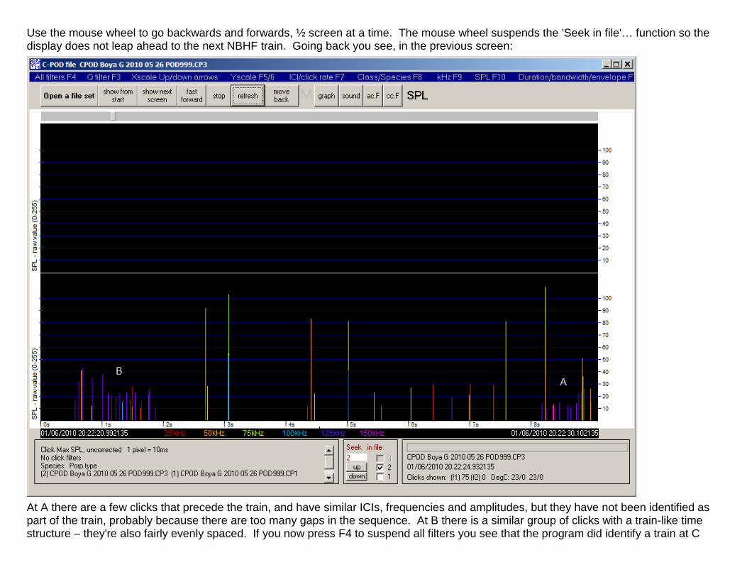
Use the mouse wheel to go backwards and forwards, ½ screen at a time. The mouse wheel suspends the 'Seek in file'… function so the display does not leap ahead to the next NBHF train. Going back you see, in the previous screen:

At A there are a few clicks that precede the train, and have similar ICIs, frequencies and amplitudes, but they have not been identified as part of the train, probably because there are too many gaps in the sequence. At B there is a similar group of clicks with a train-like time structure – they're also fairly evenly spaced. If you now press F4 to suspend all filters you see that the program did identify a train at C

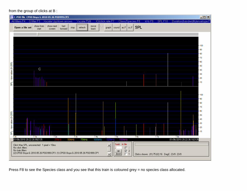
from the group of clicks at B :

Press F8 to see the Species class and you see that this train is coloured grey = no species class allocated.

At this point you are very confident that the original porpoise train is coming from a train source, as it is coherent, contains more clicks/s than the background, and similar trains and fragments of trains are showing up around the same time. The length of the clicks and lacks any wide spread of frequencies typical of dolphins. Identifying species

The KERNO classifier seeks to classify click trains into four species classes: • NBHF : long narrowband high frequency clicks, such as those produced by all porpoises ( Phocoenids ) a few dolphins and Kogia. • ‘Other cet’: short broadband clicks - BBTs = broadband transients - such as those produced by dolphins. All other cetaceans are

lumped together here at present. • Boat sonars: narrowband long clicks produced in a regular duty cycle that may contain several different ICIs. • Unclassed.

WUTS – weak unknown train sources Weak unknown train sources exist in the sea, and their characteristics can overlap those of cetaceans. They are likely to be due to some small animal, probably a small crustacean, in actual contact with the hydrophone housing. It may be scratching, scraping, singing, cleaning its teeth, or otherwise engaged. They have been seen so far in data from highly productive shallow areas: rias in the SW of Britain, the Upper Gulf of California, mangrove areas in Australia, Gulf of Alaska, and the Baltic Sea. There are regional differences in character. At present insufficient is known about them to attempt to classify them as a species. Instead the software identifies some trains as having some features of WUTS and reports on the level of such trains on the Metadata page. The risks reported are conservative i.e. they tend to over-report risks. It is possible in CPOD exe to view only those trains with some identified WUTS features, or to exclude them, but they should not be viewed as being WUTS e.g. dogs have some features of tables but are not tables. 4 legs!

Features of trains from different species:

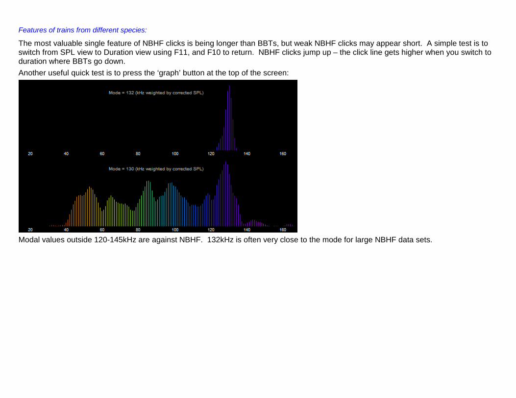
The most valuable single feature of NBHF clicks is being longer than BBTs, but weak NBHF clicks may appear short. A simple test is to switch from SPL view to Duration view using F11, and F10 to return. NBHF clicks jump up – the click line gets higher when you switch to duration where BBTs go down. Another useful quick test is to press the ‘graph’ button at the top of the screen:

Modal values outside 120-145kHz are against NBHF. 132kHz is often very close to the mode for large NBHF data sets.

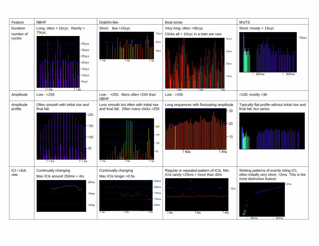
Feature NBHF Dolphin-like Boat sonar WUTS Duration number of cycles

Long: often > 15cyc. Rarely > 70cyc.

Short: few >15cyc

Very long: often >35cyc Clicks all < 10cyc in a train are rare

Short: mostly < 15cyc

Amplitude Low - >255 Low - >255. More often >255 than NBHF

Low - >255 <100, mostly <30

Amplitude profile

Often smooth with initial rise and final fall.

Less smooth but often with initial rise and final fall. Often many clicks >255

Long sequences with fluctuating amplitude

Typically flat profile without initial rise and final fall, but varies.

ICI / click rate

Continually changing Max ICIs around 250ms = 4/s

Continually changing Max ICIs longer >0.5s

Regular or repeated pattern of ICIs. Min ICIs rarely <25ms = more than 40/s

Striking patterns of evenly rising ICI, often initially very short, <2ms This is the most distinctive feature

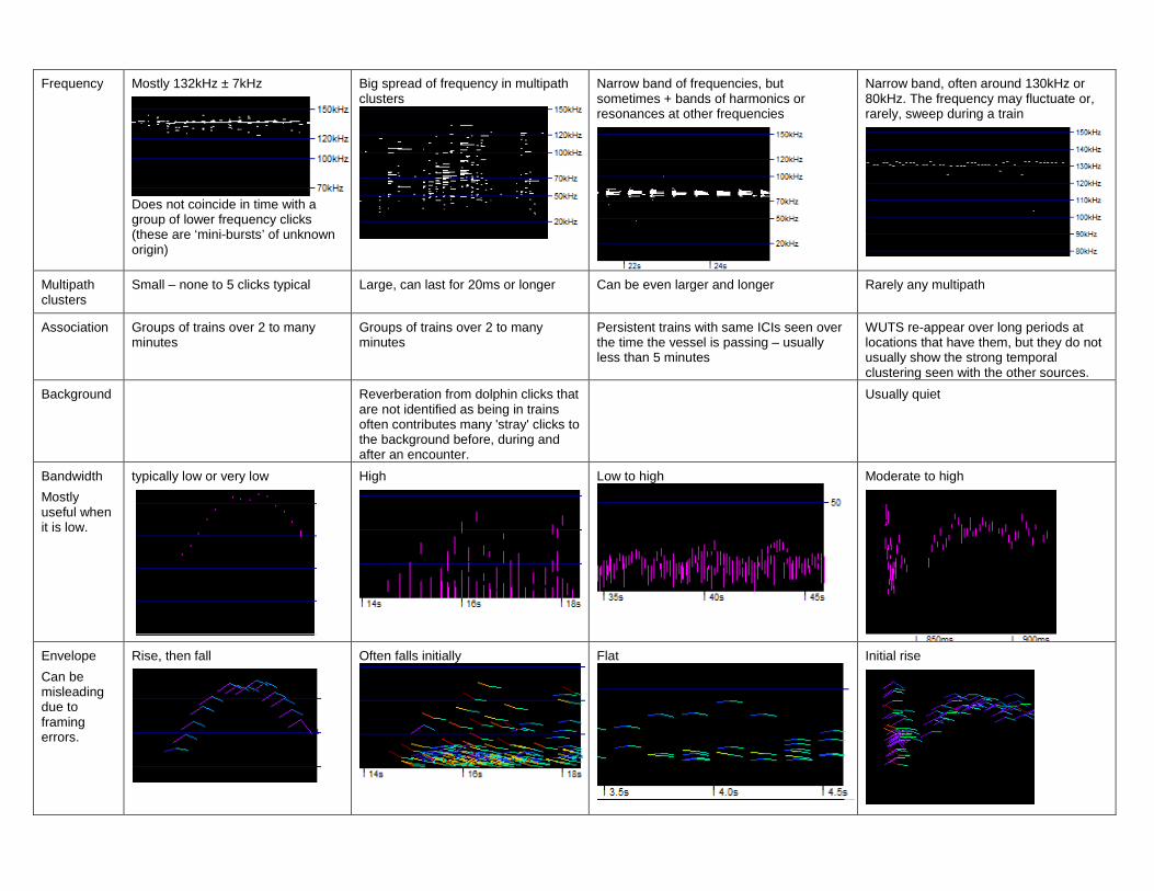
Frequency Mostly 132kHz ± 7kHz

Does not coincide in time with a group of lower frequency clicks (these are ‘mini-bursts’ of unknown origin)

Big spread of frequency in multipath clusters

Narrow band of frequencies, but sometimes + bands of harmonics or resonances at other frequencies

Narrow band, often around 130kHz or 80kHz. The frequency may fluctuate or, rarely, sweep during a train

Multipath clusters

Small – none to 5 clicks typical Large, can last for 20ms or longer Can be even larger and longer Rarely any multipath

Association Groups of trains over 2 to many minutes

Groups of trains over 2 to many minutes

Persistent trains with same ICIs seen over the time the vessel is passing – usually less than 5 minutes

WUTS re-appear over long periods at locations that have them, but they do not usually show the strong temporal clustering seen with the other sources.

Background Reverberation from dolphin clicks that are not identified as being in trains often contributes many 'stray' clicks to the background before, during and after an encounter.

Usually quiet

Bandwidth Mostly useful when it is low.

typically low or very low

High

Low to high

Moderate to high

Envelope Can be misleading due to framing errors.

Rise, then fall

Often falls initially

Flat

Initial rise

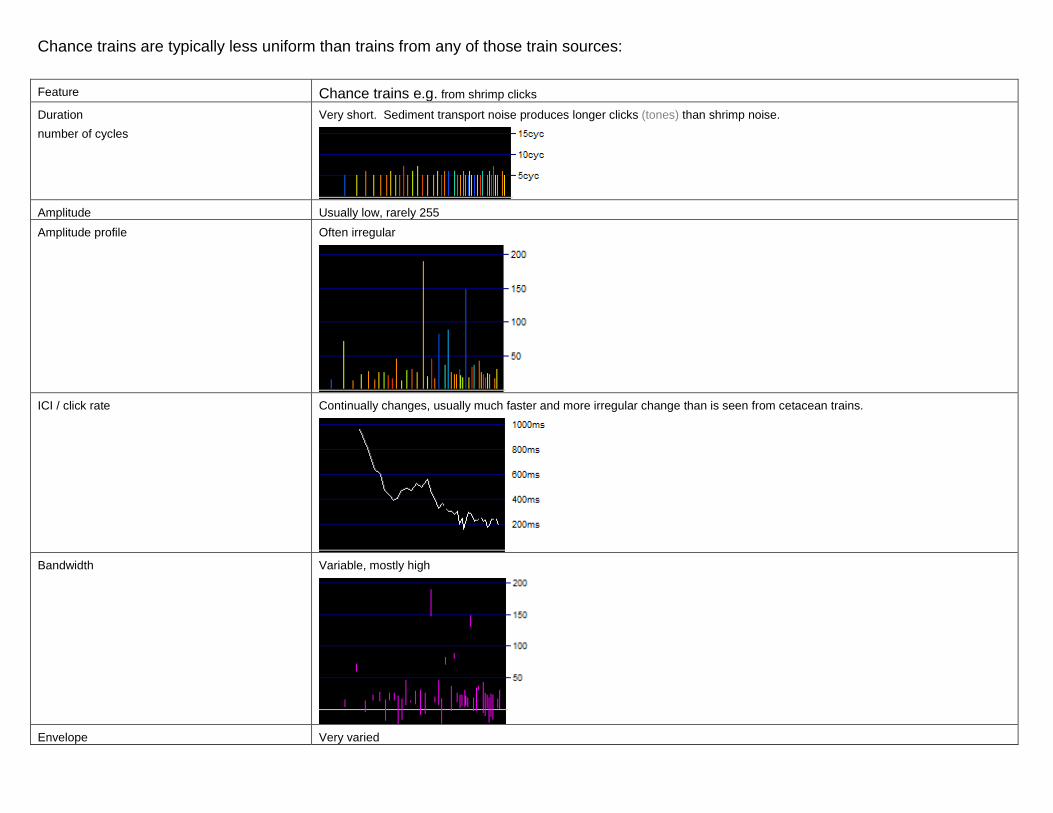
Chance trains are typically less uniform than trains from any of those train sources: Feature Chance trains e.g. from shrimp clicks

Duration number of cycles

Very short. Sediment transport noise produces longer clicks (tones) than shrimp noise.

Amplitude Usually low, rarely 255 Amplitude profile Often irregular

ICI / click rate Continually changes, usually much faster and more irregular change than is seen from cetacean trains.

Bandwidth Variable, mostly high

Envelope Very varied

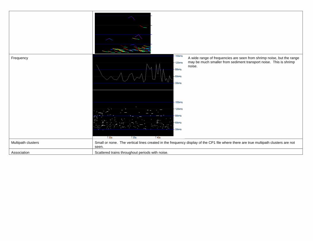
Frequency A wide range of frequencies are seen from shrimp noise, but the range

may be much smaller from sediment transport noise. This is shrimp noise.

Multipath clusters Small or none. The vertical lines created in the frequency display of the CP1 file where there are true multipath clusters are not seen.

Association Scattered trains throughout periods with noise.

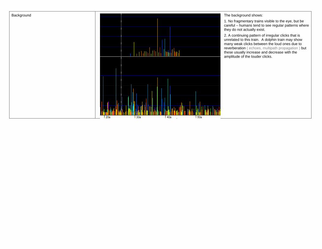
Background The background shows: 1. No fragmentary trains visible to the eye, but be careful – humans tend to see regular patterns where they do not actually exist. 2. A continuing pattern of irregular clicks that is unrelated to this train. A dolphin train may show many weak clicks between the loud ones due to reverberation ( echoes, multipath propagation ) but these usually increase and decrease with the amplitude of the louder clicks.

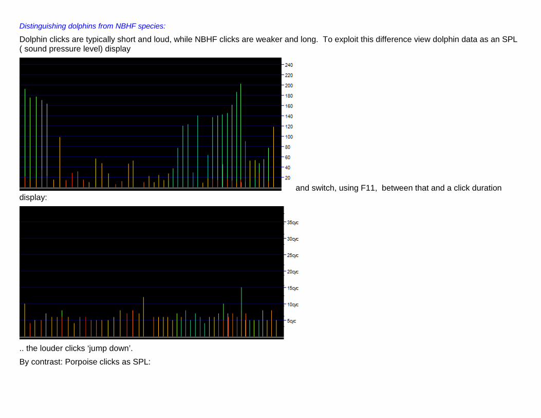
Distinguishing dolphins from NBHF species:

Dolphin clicks are typically short and loud, while NBHF clicks are weaker and long. To exploit this difference view dolphin data as an SPL ( sound pressure level) display

and switch, using F11, between that and a click duration display:

.. the louder clicks ‘jump down’. By contrast: Porpoise clicks as SPL:

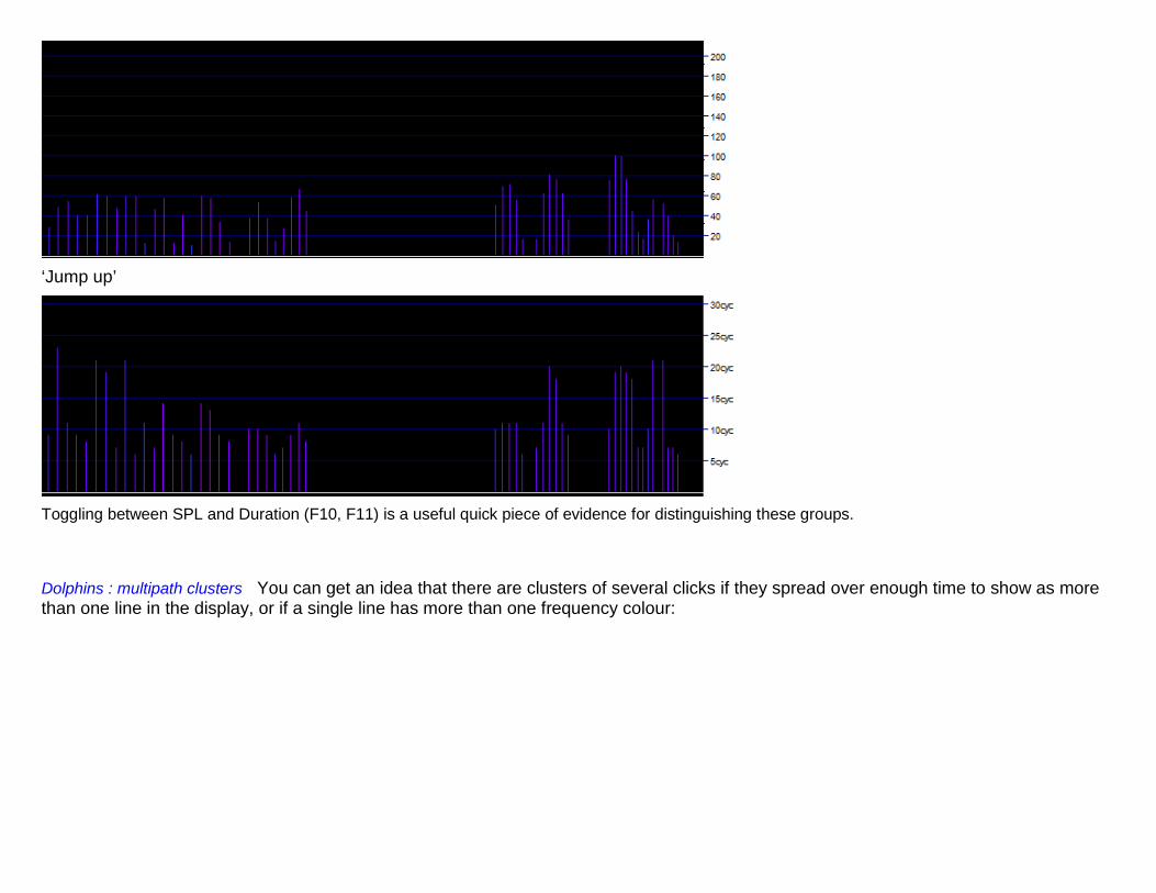
‘Jump up’

Toggling between SPL and Duration (F10, F11) is a useful quick piece of evidence for distinguishing these groups. Dolphins : multipath clusters You can get an idea that there are clusters of several clicks if they spread over enough time to show as more than one line in the display, or if a single line has more than one frequency colour:

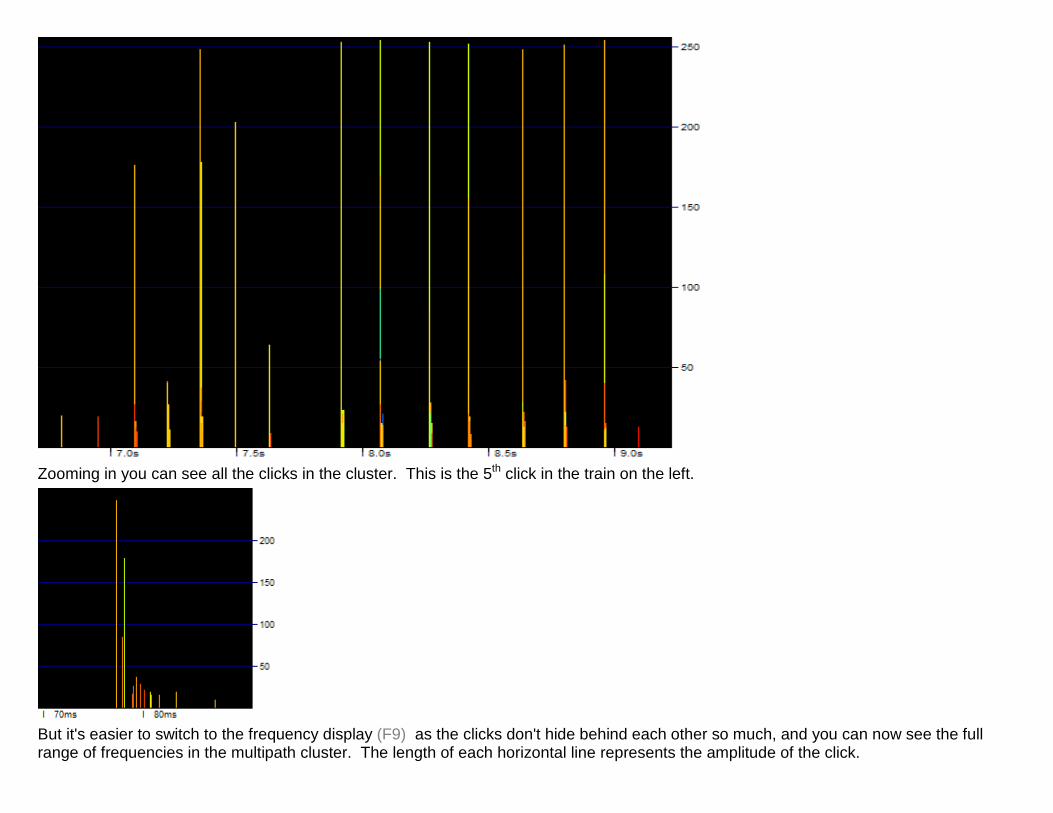
Zooming in you can see all the clicks in the cluster. This is the 5th click in the train on the left.

But it's easier to switch to the frequency display (F9) as the clicks don't hide behind each other so much, and you can now see the full range of frequencies in the multipath cluster. The length of each horizontal line represents the amplitude of the click.

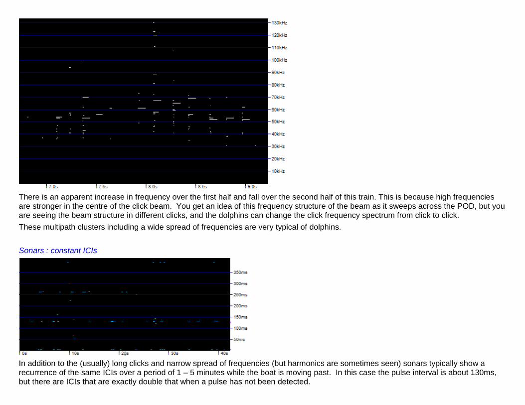
There is an apparent increase in frequency over the first half and fall over the second half of this train. This is because high frequencies are stronger in the centre of the click beam. You get an idea of this frequency structure of the beam as it sweeps across the POD, but you are seeing the beam structure in different clicks, and the dolphins can change the click frequency spectrum from click to click. These multipath clusters including a wide spread of frequencies are very typical of dolphins. Sonars : constant ICIs

In addition to the (usually) long clicks and narrow spread of frequencies (but harmonics are sometimes seen) sonars typically show a recurrence of the same ICIs over a period of 1 – 5 minutes while the boat is moving past. In this case the pulse interval is about 130ms, but there are ICIs that are exactly double that when a pulse has not been detected.

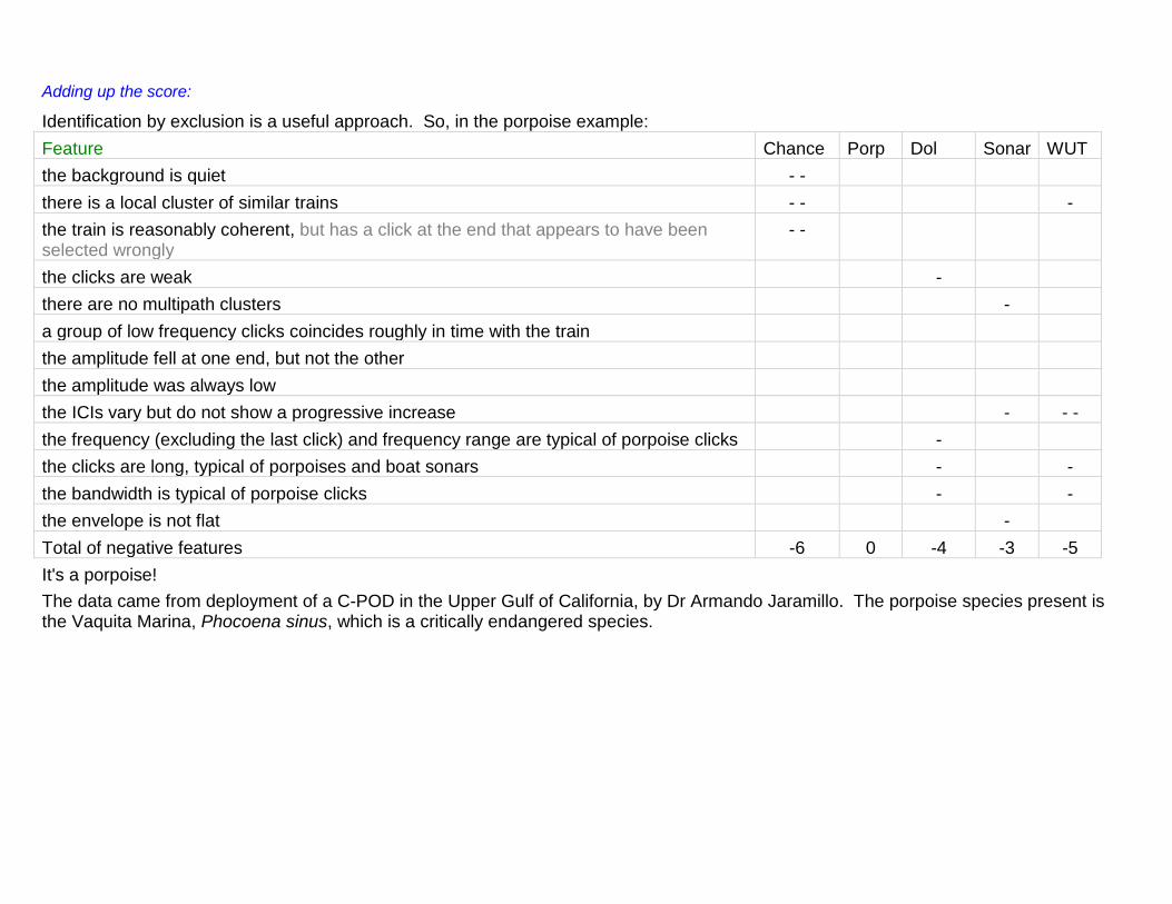
Adding up the score:

Identification by exclusion is a useful approach. So, in the porpoise example: Feature Chance Porp Dol Sonar WUT the background is quiet - - there is a local cluster of similar trains - - - the train is reasonably coherent, but has a click at the end that appears to have been selected wrongly

- -

the clicks are weak - there are no multipath clusters - a group of low frequency clicks coincides roughly in time with the train the amplitude fell at one end, but not the other the amplitude was always low the ICIs vary but do not show a progressive increase - - - the frequency (excluding the last click) and frequency range are typical of porpoise clicks - the clicks are long, typical of porpoises and boat sonars - - the bandwidth is typical of porpoise clicks - - the envelope is not flat - Total of negative features -6 0 -4 -3 -5 It's a porpoise! The data came from deployment of a C-POD in the Upper Gulf of California, by Dr Armando Jaramillo. The porpoise species present is the Vaquita Marina, Phocoena sinus, which is a critically endangered species.

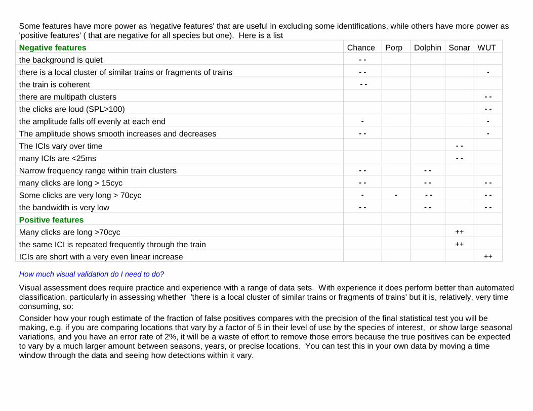
Some features have more power as 'negative features' that are useful in excluding some identifications, while others have more power as 'positive features' ( that are negative for all species but one). Here is a list Negative features Chance Porp Dolphin Sonar WUT the background is quiet - -

there is a local cluster of similar trains or fragments of trains - - -

the train is coherent - -

there are multipath clusters - -

the clicks are loud (SPL>100) - -

the amplitude falls off evenly at each end - -

The amplitude shows smooth increases and decreases - - -

The ICIs vary over time - -

many ICIs are <25ms - -

Narrow frequency range within train clusters - - - -

many clicks are long > 15cyc - - - - - -

Some clicks are very long > 70cyc - - - - - -

the bandwidth is very low - - - - - -

Positive features

Many clicks are long >70cyc ++

the same ICI is repeated frequently through the train ++

ICIs are short with a very even linear increase ++

How much visual validation do I need to do?

Visual assessment does require practice and experience with a range of data sets. With experience it does perform better than automated classification, particularly in assessing whether 'there is a local cluster of similar trains or fragments of trains' but it is, relatively, very time consuming, so: Consider how your rough estimate of the fraction of false positives compares with the precision of the final statistical test you will be making, e.g. if you are comparing locations that vary by a factor of 5 in their level of use by the species of interest, or show large seasonal variations, and you have an error rate of 2%, it will be a waste of effort to remove those errors because the true positives can be expected to vary by a much larger amount between seasons, years, or precise locations. You can test this in your own data by moving a time window through the data and seeing how detections within it vary.

Tips

Seeking NBHF species: View either SPL or N cycles (duration). Toggle between the two F10 / F11to see the NBHF clicks go up where BBT go down. F9 to show frequency is useful to see the narrow frequency range of the train. Use the frequency graph to get the mode. Seeking BBT species: View SPL and toggle to frequency F10 / F9 to see the wide frequency spread. Try the ‘shade Ncyc’ and ‘shade BW’ options to give a bit more information in SPL view.

Good practice

‘When in doubt, chuck it out’. In a low density area a low rate of false positives is much more damaging that the loss of sensitivity from setting higher criteria, as it can generate a thin spread of detections in places or times never visited by the species.

Editing CP3 files by marking false positives

If you decide you do need to remove false classifications you will already be excluding all except Hi and Mod quality trains. Then follow these steps:

• Open the file pair, and set ‘Seek ..’ as above. • Set the time resolution to 10ms, and parameter to SPL or Duration. Either shows you the frequency as a colour, and you may find

one more informative, but you can switch between them using F9 (frequency) or F10 (SPL). • Move from train assessing them as above. • To mark a false positive put the mouse pointer to the left of the earliest click in the train, right-click and select the ‘Mark this train’.

The edit is recorded in the Results. • or ‘Mark this minute’ with the mouse pointer anywhere in the minute.

You may mark true trains if they are far fewer than false trains to reduce the time spent marking trains. You can remove all marks via the ‘view+’ page.

To upgrade or not to upgrade?

Rejecting trains is 'downgrading'. Changing the species class to a cetacean species group is 'upgrading'. It is much better to use only downgrading if you have enough data, as this is quicker and the subjective element in the process is less than for upgrading, making it easier to reproduce the results accurately with a different operator. But: it's best to avoid all editing, if the error rate is low enough. Then you, or others, can then apply exactly the same detector in future, and you have not committed future time to making future results comparable with present results.

Finding false negatives – and pinger data

The extreme end of upgrading is to search for trains that have been missed. This is the most subjective editing task and should not be done unless it is really unavoidable. This may be the case where the data contains pinger sounds that are identified as sonars in a very large proportion of minutes. The software detects these ‘sonars’ and their presence creates a bias in the species classifier against cetacean species identification. Seeking NBHF species in files with sonars:

To avoid this bias you can filter the CP1 file for clicks with NBHF features that are not found in the clicks from the pingers or sonars logged. This requires careful scrutiny of the whole data set.

Seeking BBT species in files with sonars: BBT clicks are less distinctive than NBHF clicks and the discrimination task is harder and depends on identifying features not possessed by the pinger or sonar but present in the ‘dolphin’ encounters.

False negatives

Don’t get greedy about false negatives! Let them go! Detection functions in line and point transect methods represent the spatial distribution of false negatives. They are often simply equivalent to having a slightly less sensitive detector, or slightly fewer detectors. If you go to a lot of trouble to upgrade them to true positives be sure to analyse your results with and without that editing, as you will then most likely find that all your effort left you with the same conclusions, but the process was time consuming, introduced subjectivity and consequently lost some reproducibility.

Some advanced display tools

It is useful to sometimes to see how the number of clicks in trains matches, or not, the number of raw clicks, but the latter may be off the

scale. You can downscale the CP1 file click counts by increasing the value ‘40’ to, say 400. Comparing edited files: You can compare any edited CP3 files with the original CP3 by opening up to 3, setting the time scale to 100ms or less and pressing Shift C This sets 'compare files' and the display will skip through screens until it finds a difference between and 2 CP3 files that are open. Fast forward review: Open a file set and view Sp class at 10ms. Press Fast Forward and it will skip repeatedly between screens with detections matching your filter settings. Each time you press Fast Forward the speed doubles. Sit back from the screen and concentrate on the lower (CP1) panel. This gives a very useful fast survey of a lot of data. You may see some anomalous patterns that merit investigation during your validation process.

Sampling detections in a file

Start from the beginning and view the next 10 trains, then drag the slider bar at the top about 10% of the way through the file and view another ten trains. Repeat this until you have viewed 100 trains, noting the number of false positives. Ignore false negatives. If there is a particular source of false positives, such as periods of boat sonar activity or dolphin activity you may need to change, or increase, the sampling regime to ensure that these are not missed. To detect such anomalies select a time scale of 30min, then select the parameter ‘Frequency’ then the parameter ‘Sp class’. As the CP1 file contains no species class information it show the last parameter you selected that it does contain, so you get the frequency distribution of the raw data in the lower panel and the species in the upper panel:

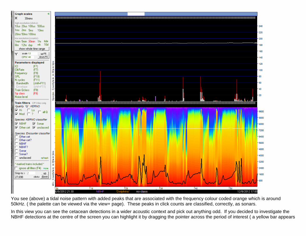
You see (above) a tidal noise pattern with added peaks that are associated with the frequency colour coded orange which is around 50kHz. ( the palette can be viewed via the view+ page). These peaks in click counts are classified, correctly, as sonars. In this view you can see the cetacean detections in a wider acoustic context and pick out anything odd. If you decided to investigate the NBHF detections at the centre of the screen you can highlight it by dragging the pointer across the period of interest ( a yellow bar appears

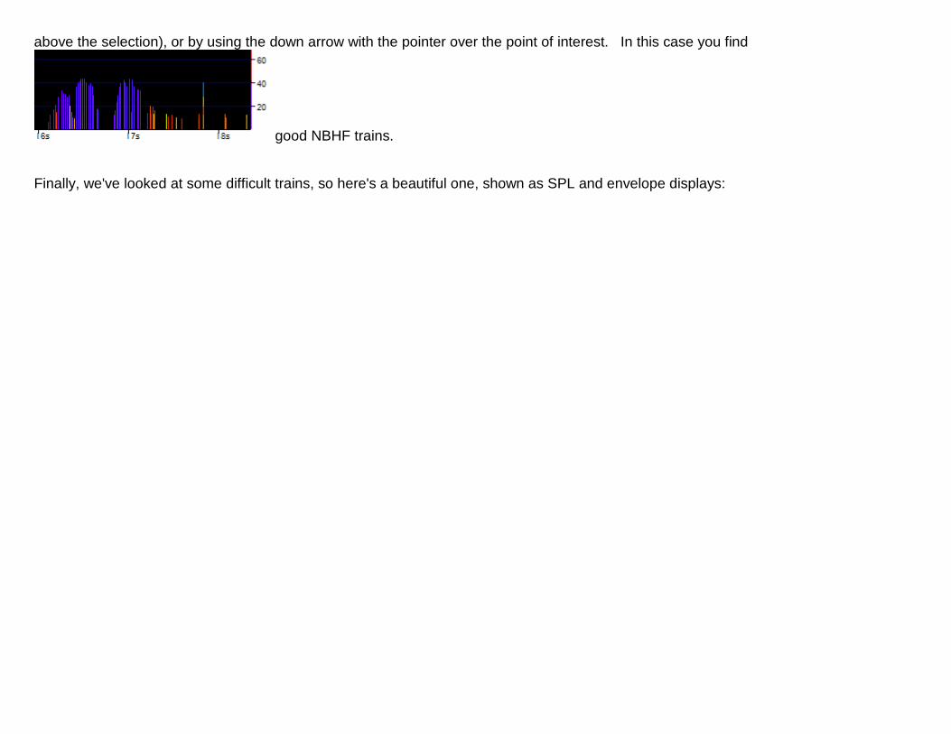
above the selection), or by using the down arrow with the pointer over the point of interest. In this case you find

good NBHF trains. Finally, we've looked at some difficult trains, so here's a beautiful one, shown as SPL and envelope displays:

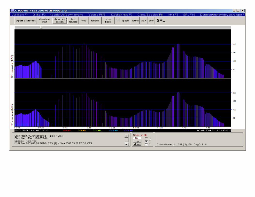
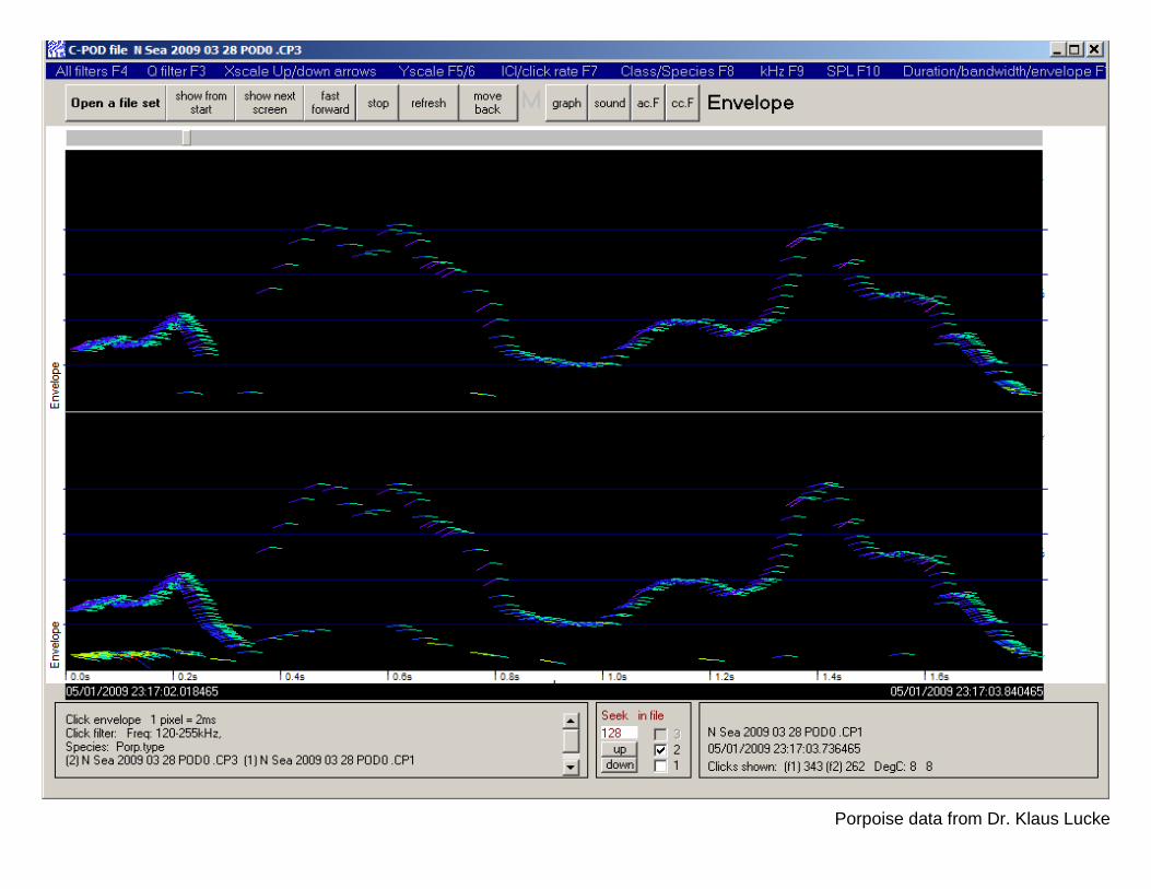
Porpoise data from Dr. Klaus Lucke