by kevin heisler - stetson universityefriedma/research/kheisler.pdf · kevin heisler a senior...

MODELING LOWER BOUNDS OF WORLD RECORD RUNNING TIMES

By

KEVIN HEISLER

A SENIOR RESEARCH PAPER PRESENTED TO THE DEPARTMENT OF MATHEMATICS

AND COMPUTER SCIENCE OF STETSON UNIVERSITY IN PARTIAL FULFILLMENT OF

THE REQUIREMENTS FOR THE DEGREE OF BACHELOR OF SCIENCE

STETSON UNIVERSITY

2009

2

ACKNOWLEDGMENTS

I would like to thank my advisors Dr. John Rasp and Dr. Erich Friedman for

making themselves available to assist me and guide me in this research. I want to say

thanks to my brother and roommate Brian Heisler, and to my other roommates Thomas

Parks and William Wood for having the intellectual capacity to help me hone my

mathematical skills when I am struggling, and also provide the balance between

schoolwork and life. Thanks to my parents for providing for me while I am at school so I

can focus on intellectually bettering myself.

3

TABLE OF CONTENTS

ACKNOWLEDGEMENTS ------------------------------------------------------------------ 2

LIST OF TABLES ------------------------------------------------------------------------------ 5

LIST OF FIGURES ----------------------------------------------------------------------------- 6

ABSTRACT ------------------------------------------------------------------------------------- 7

CHAPTERS

1. INTRODUCTION --------------------------------------------------------------------- 8

1.1. Beginning Models ---------------------------------------------------------------- 8

1.2. Predictive Models ---------------------------------------------------------------- 8

1.3. Alternative Models --------------------------------------------------------------- 12

1.4. Preview ---------------------------------------------------------------------------- 12

2. UPDATING THE EQUATIONS ---------------------------------------------------- 14

2.1. Gathering the Data ---------------------------------------------------------------- 14

2.2. Examining Lucy’s Exponential Equation -------------------------------------- 15

2.3. Power Model ----------------------------------------------------------------------- 20

3. DISTRIBUTION OF THE MINIMA ----------------------------------------------- 25

3.1. Gamma Distribution -------------------------------------------------------------- 25

3.1.1. Method of Moments ---------------------------------------------------- 26

3.1.2. Goodness of Fit ---------------------------------------------------------- 28

3.1.3. Maximum Likelihood Estimators ------------------------------------- 30

3.1.4. Expanding the Sample -------------------------------------------------- 31

4. ORDER STATISTICS ---------------------------------------------------------------- 36

4.1. Deriving the Minimum of the Order Statistic -------------------------------- 36

4.2. A New Sample -------------------------------------------------------------------- 38

4.3. Equating the Sums ---------------------------------------------------------------- 41

4.3.1. Checking the Original Data Set --------------------------------------- 41

4.3.2. Checking the New Data Set ------------------------------------------- 43

5. SHORTER DISTANCES ------------------------------------------------------------ 45

5.1. Revisiting the Gamma Distribution -------------------------------------------- 45

5.2. Ordering the Data ---------------------------------------------------------------- 47

5.2.1. Kolmogorov – Smirnov Test ------------------------------------------ 48

5.3. Variables in Decreasing Time -------------------------------------------------- 50

5.3.1. Identifying the Variables ----------------------------------------------- 50

5.3.2. Quantifying the Variables --------------------------------------------- 53

4

6. FUTURE WORK ---------------------------------------------------------------------- 57

6.1. Generalized Gamma Distribution ---------------------------------------------- 57

6.2. Shorter Distances ---------------------------------------------------------------- 57

REFERENCES ---------------------------------------------------------------------------------- 59

BIOGRAPHICAL SKETCH ------------------------------------------------------------------ 61

5

LIST OF TABLES

TABLE

1. Chatterjee Estimates and Actual Times ---------------------------------------- 11

2. Number of Data Points -------------------------------------------------------------- 14

3. Exponential Model Parameter Estimates for One Mile ----------------------- 18

4. Exponential Model Parameter Estimates for 400M ---------------------------- 18

5. Exponential Model Parameter Estimates for 800M ---------------------------- 19

6. Exponential Model Parameter Estimates for 5000M -------------------------- 19

7. Exponential Model Parameter Estimates for Marathon ----------------------- 19

8. Power Model Parameter Estimates for 400M ----------------------------------- 20

9. Power Model Parameter Estimates for 800M ----------------------------------- 20

10. Power Model Parameter Estimates for One Mile ------------------------------ 20

11. Power Model Parameter Estimates for 5000M --------------------------------- 21

12. Power Model Parameter Estimates for Marathon ------------------------------ 21

13. Comparison of Estimates: Exponential Model vs. Power Model ----------- 22

14. Comparing Chi-Square Statistics ----------------------------------------------- 31

15. Comparing Estimates ---------------------------------------------------------------- 35

16. Parameter Values by Year ------------------------------------------------------- 35

17. Derivation of Minimum by Year -------------------------------------------------- 37

18. Original Parameter Values ------------------------------------------------------- 42

19. Adjusting α ------------------------------------------------------------------------- 42

20. Adjusting θ ------------------------------------------------------------------------- 42

21. Adjusting n ------------------------------------------------------------------------- 42

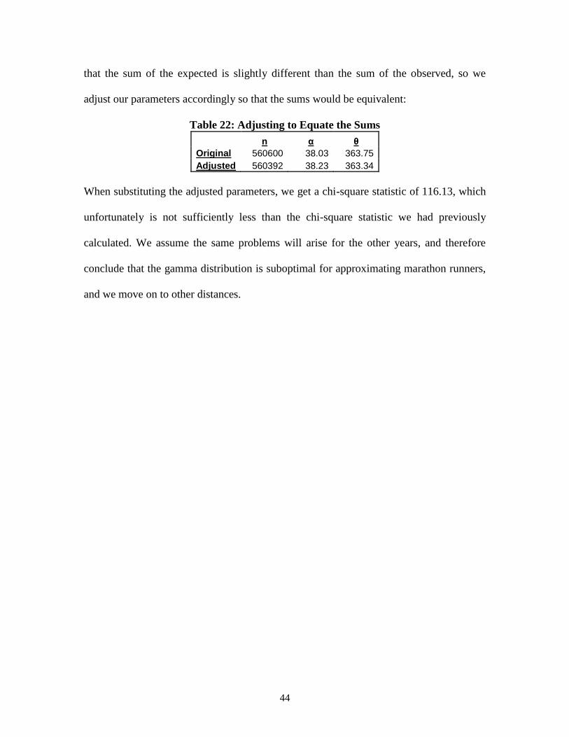
22. Adjusting to Equate the Sums --------------------------------------------------- 44

23. Variables for 100m ---------------------------------------------------------------- 53

24. Variables for 200m ---------------------------------------------------------------- 54

25. Variables for 400m ---------------------------------------------------------------- 54

26. Variables for 800m ---------------------------------------------------------------- 54

27. Variables for 1500m ---------------------------------------------------------- ---- 54

28. Variables for One Mile ----------------------------------------------------------- 55

29. Variables for 5,000m --------------------------------------------------------- ---- 55

30. Variables for 10,000m -------------------------------------------------------- ---- 55

31. Variables for Half-Marathon ------------------------------------------------ ---- 55

32. Variables for Marathon ------------------------------------------------------- ---- 56

6

LIST OF FIGURES

FIGURE

1. Graph of Minimum Sum of Squares Based on Parameter Estimates ------ 17

2. Power Function for Marathon Best of Year Data ------------------------------ 22

3. Scatter Plot of Residuals from Marathon Best of Year Data ----------------- 23

4. Histogram for 2008 Boston Marathon Data ------------------------------------- 26

5. Histogram for 2008 NYC Marathon Data --------------------------------------- 26

6. Histogram of Combined 2008 Boston and NYC Marathons ---------------- 26

7. Combined Histogram of Expected and Observed Frequencies for 2008

Boston and NYC Marathons --------------------------------------------------- 29

8. Histogram of the Data ------------------------------------------------------------ 33

9. Observed and Expected Data ---------------------------------------------------- 34

10. Graph of the Probability Density Function -------------------------------------- 37



13. Marathon Histogram ----------------------------------------------------------------- 45

14. 100m Histogram ---------------------------------------------------------------------- 45

15. 200m Histogram ---------------------------------------------------------------------- 46

16. 400m Histogram ---------------------------------------------------------------------- 46

17. 800m Histogram ---------------------------------------------------------------------- 46

18. 1500m Histogram -------------------------------------------------------------------- 46

19. One Mile Histogram ----------------------------------------------------------------- 46

20. 5000m Histogram -------------------------------------------------------------------- 46

21. 10000m Histogram ------------------------------------------------------------------- 47

22. Half-Marathon Histogram ---------------------------------------------------------- 47

23. Graphing the 100m Times from 2008 in Ascending Order ------------------ 47

24. Graphing the 100m Times for All Years in Ascending Order --------------- 48

25. Graphing the Half-Marathon Times for All Years in Ascending Order --- 49

26. Graphing the Mile Times for All Years in Ascending Order ---------------- 50

7

ABSTRACT

MODELING LOWER BOUNDS OF WORLD RECORD RUNNING TIMES

By

Kevin Heisler

April 2009

Advisors: Dr. John Rasp and Dr. Erich Friedman

Department: Mathematics and Computer Science

Fifty years ago, the first truly predictive model was developed for estimating a

lower bound on a world record (the men’s one mile record). This sparked an interest in

modeling world record running times which has, in the past decade, faded. Then in 2008

at the Beijing Olympics 21 year old Usain Bolt broke the world record for both the 100

meter and 200 meter sprints. With his remarkable performance, Bolt not only established

himself as one of track and field’s premier athletes, but he reignited the debate over how

low the world records for these events will ultimately fall. This paper presents several

mathematical models for estimating a lower bound on world record running times for

various distances ranging from the 100 meter sprint to the marathon. The models will use

regression and order statistics to model the lower bounds.

For equations that require a solution to a system of equations that is not in closed

form, we will be using numerical analysis methods on Mathematica® to estimate

parameters. We will also use Mathematica® in solving linear systems for polynomial

equations. These models will help us gain some insight into which records, if any, have

already reached their pinnacle, and which records we can expect to be broken in the near

future.

8

CHAPTER 1

INTRODUCTION

1.1 BEGINNING MODELS

In 1913, the International Amateur Athletic Foundation was founded as a

committee that would keep official statistics on running records. However, even before

the IAAF was founded, mathematicians had begun constructing models to predict how

low certain running times would fall. In 1906 Kennely [7] used time-distance analysis to

plot time based on a given distance for distances ranging from 100 yards to 10 miles. He

let d be the distance of the race, in meters, and t the time the race took, in seconds. This

yielded a log-log equation of:

log(t) = 1.125log(d) – 1.236

which, when solved for time t, gives:

t = 0.0581d1.125

Though Kennelly did not construct this model strictly for predictive purposes, he did

make a prediction for the ultimate world record in the mile run, which he estimated to be

3:58.1. The current world record for the men’s one mile is 3:43.13.

1.2 PREDICTIVE MODELS

The first mathematical model constructed strictly for predictive purposes was

done in 1958 by Lucy [8], who used the year to derive an exponential function for

predicting the ultimate time in the one mile run, where tn is the time, in seconds, for the

mile record in the year (1950 + n), and k and a are estimated parameters:

tn = t0 + kan

9

Using this model, Lucy predicted an ultimate best time for the mile of 3:38, which is

close to the record time now, fifty years later, of 3:43.13.

Just a couple of years after Lucy developed his model, Deakin [5] developed two

distinct models using data from the years 1911 – 1965 in which world records were

broken. For both models tn is the time for a given year n years after 1911 in which a

world record was set, α and β are parameters estimated through iterative methods, and γ

(and in the second equation δ) are parameters estimated by looking at the plot and

guessing the best fit curve:

tn=e - (n-1)

+

tn=-(2 /) arctan ( (n-1)+)

While it is clear that the arctan function was used because of its decaying shape, it seems

illogical to use this equation because there is no reason to believe that running time data

would behave according to an arctan function.

The second equation was also used for backward extrapolation to estimate an

upper bound on what the fastest humans have always been capable of running in the mile,

which Deakin estimated to be 5:00. Though both equations were crudely derived, both

yielded the same lower estimate for the mile of 3:34, which is very close to Lucy’s

prediction of 3:38, and nine seconds from the current world record of 3:43.13.

In 1983 Schultz and McBryde [12] devised four unique models for predicting

record performances in track and field. These models were derived by examining the best

performance of the year for every year from 1900-1982. Subsets of these years were also

fitted to the models to determine the effects of world events, such as WWI and WWII,

but no significant influences were found. The authors found that all four models were

10

approximately equally effective in fitting data from the shorter distances, but the model

that best fit longer distances was an exponential model where tn is the predicted time for a

given year that is n years after 1899, α is the limit of tn as n → ∞, and β and γ are

estimated parameters, with the restriction that γ must be negative:

tn=+e n

The unique characteristic about this equation is that it models all track and field events,

not just the running events. The only change to be made between running events and field

events is the sign on β, which is positive for running events. Using their equation, Schutz

and McBride estimated the ultimate mile time to be 3:28.5, compared to the current world

record of 3:43.13 today.

In 1993 Schutz and Liu [13] reformatted this equation to fit a larger, more current

sample, and used it for predictive purposes of one event, the men’s 1500M. This new

model, called the Random Sampling Model, works under the assumption that

improvement has stabilized, and that a new record would be an outlier of a data sample.

We will consider this idea in Chapter 3.

Chatterjee and Chatterjee [4] developed a model to predict ultimate times based

on past Olympic performances. They used the winning times for the 100m, 200m, 400m

and 800m races at the Olympics from 1900 – 1976 to look at the effects of Olympic year

and race distance on time. In their equation, i refers to the ith Olympics within the range

(1900 – 1976) and j refers to the jth event, with the events numbered 1 – 4 from shortest

to longest distance. The variable d represents the actual distance of the race, measured in

meters:

log(tij) = 0.249 + 0.150-0.069j

– 0.00263 dj + 0.229√dj

11

Though the model was developed for the prediction of lowest times, the authors

were more interested in predicting the times at the next Olympics, which would have

been the 1984 Olympics in Los Angeles. The lowest times for the four events were not

reported, but their predictions and the observed times for the 1984 Olympics were:

Table 1: Chatterjee Estimates and Actual Times

Race Prediction Actual

100m 9.98 9.99

200m 19.80 19.80

400m 44.77 44.27

800m 104.62 103.00

Whereas Schutz and McBryde’s model applied to all events from track and field,

Morton [10] developed a model to predict times which included a unique factor in shorter

track events: lane allocation. Time was determined by factoring the effects of gender (G),

distance of the race (D), lane (L), and hurdle effects (H) (which is obviously not

applicable in all races), and the equation Morton arrived at is:

T = 21.71 + 26.75D + 4.52H -1.87G –

2.64DG – 1.48HG + 0.37DL – 0.30HL – 0.18GL + 0.84HL2

With this equation, Morton analyzed world record performances in reference to lane

allocation. His study found no significant pattern in lane allocation and world record

performance for the events, suggesting that for the races where lane assignment is

mandatory throughout the entire race, lane allocation does not significantly affect

performance. His results contradict the two theories that the outer lanes have an

advantage due to the more gradual curvature, and the inner lanes have an advantage

because of the ability to see the other competitors.

12

1.3 ALTERNATIVE MODELS

In addition to predictive mathematical models, where the main focus is to minimize

time over a given distance, there have been several attempts to formulate a predictive

model on the upper bound of maximum speed over a given distance.

One of the most prominent studies for this subject was done by Joseph Keller [6]

in 1973. In trying to determine the optimal strategy for pacing in a race of a given

distance so that time is minimized, Keller examined oxygen flow and the amount of

energy provided from this flow, resistive forces per unit mass, force exerted by a runner,

and velocity to calculate the maximum distance such that maximum velocity can be

maintained. Keller calculated this value to be 291 meters. This suggests that for all

distances in our study, with the exception of the 100M and 200M sprints, a pacing

strategy must be utilized to minimize time.

As a result of this discovery, equations for pacing strategies have been developed to

minimize the effects of fatigue during a race of a longer distance. Frank Mathis [9]

examines Keller’s optimal velocity equation and modifies it to include a variable for

oxygen deficit during a race.

1.4 PREVIEW

The previously mentioned studies all contribute to the idea of finding a lower bound

on running times. Some of the models extrapolate known data to predict future outcomes.

In predicting, there has been a wide range of ultimate record times – some of which have

been already broken, some of which will seemingly never be broken, and some of which

are just small percentage points away from being broken. Other models explain the effect

some variables have on running time or velocity, including resistive and propulsion

13

forces [2], VO2 max, fatigue [3,6], pacing [1], and oxygen consumption. Though each

contribution is different, all of the models will be considered as a unique equation is

constructed for predicting a lower bound on world record running times.

14

CHAPTER 2

UPDATING THE EQUATIONS

2.1 GATHERING THE DATA

We used the International Amateur Athletic Foundation to gather our data [16],

which includes exclusively men’s data as of now. We have compiled three classes of

data: The first list is a list of the best recorded times in history for a given event. The next

list is a list of the best time of the year for the event, and the final list is a list of the world

record progression for the event. The world record list includes only the times that better

the previous world record; the instances when the world record time was matched for an

event were not included in the data set. The following figure gives the number of data

points gathered for each event:

Table 2: Number of Data Points

Event # Data Overall Best # Data Best of Year # Data WR Prog.

100m 555 34 19

200m 264 34 21

400m 178 33 22

800m 167 32 17

1500m 253 29 33

One Mile 178 32 31

5,000m 296 22 35

10,000m 160 25 38

Half-Marathon 170 19 17

Marathon 152 18 35

It is to be noted that, for the best time of the year data, there are some years for

which the best time was not available. For the world record times, some data sets have

multiple values for the same year, due to the fact that the world record was broken more

15

than one time in the same year. There are also many instances when there are several year

gaps in the world record data. For example, the men’s one mile world record was broken

three times in 1981, but has only been broken three times since then, most recently in

1999.

As of now, we are only looking at the data from 5 events: 400m, 800m, One Mile,

5000m, and Marathon. The other distances will be examined at a later time.

2.2 EXAMINING LUCY’S EXPONENTIAL EQUATION

The first family of equations we are looking at is the exponential decay function.

We focus on the form displayed by Lucy’s equation. Recall that tn is the best time of the

year, and is known data; t0 is the lower bound on the time; n is the number of years after

1950; and k and a are parameters to be estimated:

Using the data from 1950 – 1958, Lucy found a lower bound for the men’s one

mile time of 218 seconds, or 3:38, which is approximately five seconds faster than the

current world record of 223.13 seconds, or 3:43.13.

Using this general form of the equation, we use the best mile times from the years

1967 – 2007 to estimate the lower bound, t0. We have reindexed the value of n to be the

number of years since 1967 for our version of the model. We also will estimate the

parameters k and a.

To find these estimates, first we define an equation to find the sum of squares for

the data points:

16

We are trying to minimize the value of the sum of squares equation, so we take

the partial derivative of the equation with respect to each variable and set each of these

derivatives equal to zero. We end up with a system of three equations and three

unknowns, so now we solve for the unknowns. Unfortunately, the system of equations

does not have a closed-form solution. Thus, we must use a numerical method to

approximate a solution. We use the FindRoot function on Mathematica to approximate

the values for the parameters. Because this is a numerical process, we are required to

initialize values for the parameters. We started by using the estimates Lucy was able to

find in his equation:

FindRoot[{SSA = = 0 , SSK = = 0 , SST = = 0} , {a , 0.933} , {k , 31} , {t , 218}]

However, new estimates were not able to be found after 10,000 iterations, so the original

estimates were adjusted. The value for k tended to be much lower than Lucy’s estimate as

it was adjusted, and the value for a tended to be slightly higher, so the original guesses

were adjusted accordingly. Note that the value for a must be less than one in order for the

equation to approach a lower bound. Using the new initial values, the numerical

approximation converged in 9 iterations:

FindRoot[{SSA = = 0 , SSK = = 0 , SST = = 0} , {a , 0.94} , {k , 10} , {t , 218}]

{a = 0.947 , k = 6.079 , t = 225.89}

Our value for the lower bound, 225.89 seconds, is approximately eight seconds

slower than the bound Lucy found. Our value for a is approximately the same, but our

value for k is significantly different. This difference can be explained by the role the

17

parameter plays in the equation. The parameters k and a determine the rate of decay for

the function. Because our value for a is similar to Lucy’s, we only consider the

differences in k. In Lucy’s equation, the domain was from [0, 8], whereas in our equation,

the domain goes from [0, 40]. This allows for a more gradual decay, provided that the

absolute decays of the two equations are comparable. For Lucy’s equation, exact data

could not be found, but based on estimates using the world record progression, we

approximate the time decay from 1950 – 1958 to be ten seconds. The decay from 1967 –

2007 for our equation was approximately eight seconds. Thus the decay is more gradual,

and the curve is less steep compared to Lucy’s as shown by the lower k estimate in our

equation.

If we replace one of the variables for which we solved into the sum of squares

equation, we can graph the function for the other two variables to show that the minimum

exists at the convergent values. So we plug t0 into the equation and graph it:

Figure 1: Showing the minimum of the sum of squares graphically

0.85

0.9

0.95

1

2

4

6

100

200

300

400

0.85

0.9

0.95

1

2

4

6

This shows that the minimum occurs at the estimated parameters. Using these parameter

estimates, we can calculate the sum of squares and variance for our data.

SS = 88.066 σ2 = 3.037

18

If we look at smaller subsets of the data, we can see how the times are behaving

over different intervals of time and use this information to improve our overall model. So

we repeat the sum of squares process for smaller subsets of the data, as well as for the

world record progression:

Table 3: One Mile: Current World Record is 223.13 seconds (3:43.13)

Subset of Years k a t0 SS Variance

1967 – 2008 6.078 0.947 225.89* 88.066 3.037

1967 – 1987 11.941 0.977 220.00* 12.263 1.226

1979 – 1989 0.742 0.198 228.25 12.999 1.625

1979 – 2000 11.300* 0.977 220.66 56.256 2.961

WR progression 1.800 0.037 237.20 2417.440 86.337

In some instances (indicated by a *), the system of equations was not converging

after 40,000 iterations. However, one of the parameters would stay approximately the

same as the initial guesses were altered; thus that approximate value was substituted into

the original equation, and the system became a system of two equations and two

unknowns, which converged.

The exponential model fits relatively well for the subsets of years, but not for the

world record progression. This trend was evident in the four other distances for which

this method was used:

Table 4: 400m: Current World Record is 43.18 seconds


1968 – 2008 3.479 0.993 41.05 4.983 0.166

1968 – 1988 -0.490 0.001 44.35 1.594 0.159

1988 – 2008 2.497 0.351 43.79 2.3936 0.141

WR progression 2.662 0.208 45.14 18.790 1.566

19

Table 5: 800m: Current World Record is 101.11 seconds (1:41.11)


1973 – 2008 1.073 0.784 102.75 13.919 0.480

1973 – 1988 1.249 0.825 102.58 4.639 0.464

1993 – 2008 1.270 0.272 102.61 5.457 0.455

WR progression 0.297 0.031 106.19 233.264 16.661



1981 – 2008 30.446 0.959 755.34 900.699 47.405

WR progression 0.063 0.037 808.48 39165.100 1223.910

Table 7: Marathon: Current World Record is 7439 seconds (2:03:59)


1985 – 2008 80.545 0.840 7580.22* 58,362.500 3,890.830

WR progression 3490.510 0.979 7098.28 89,286,820.000 2,880,220.000

Note that in the 400m data, the 1968 – 1988 subset has a k value of -0.49 and an a

value of 0.001. Because the value of a is small, the equation approaches the lower bound

quickly, and the sign on k becomes insignificant. The world record data has the worst fit

for this model in all of the distances examined thus far. This should be expected though,

as the model was made for the best time of the year data, not world record progression.

In many instances, the lower bounds estimated are actually slower than the

current world record times. This does not mean that they are inaccurate though, as the

variance in the data could account for the differences in the times. However, we look at a

different model to see if there is a better fit and to see if we can get different lower

bounds. The next model we examine is the power model.

20

2.3 POWER MODEL

The family of equations we look at in the power model has tn as the best time of

the year, t0 as the lower bound on the world record time, n as the number of years after a

given year, k and a as parameters to be estimated, and has the form:

We use the same data that was used in finding the exponential equations. When finding

the parameters and lower bound, we use the same process as in the exponential equation.

The only difference is that this family of equations is polynomial and has a closed form

solution. We can use a linear solve method, rather than a numerical approximation

method, to solve for the parameters. We use the NSolve function in Mathematica to find

the values of the parameters and the lower bound.

Table 8: 400m: Current World Record is 43.18 seconds


1968 – 2008 -6.185 6.312 43.72 4.782 0.159

WR progression -145.996 151.660 42.14 2.240 0.187



1973 – 2008 -1.945 3.010 102.62 12.117 0.418

WR progression -199.454 211.441 99.91 17.152 1.225

Table 10: One Mile: Current World Record is 223.13 seconds (3:43.13)


1967 – 2007 -34.641 39.817 225.91 87.477 3.017

WR progression -17,815.200 1,868.500 208.55 100.566 3.592

21



1981 – 2008 -49.836 68.099 766.39 1108.200 58.326

WR progression -66,277.000 7,164.780 709.16 3906.020 122.063

Table 12: Marathon: Current World Record is 7439 seconds (2:03:59)


1985 – 2008 -489.252 584.898 7527.12 46,589.500 3,105.970

WR progression -285,875.000 58,118.000 7131.64 1,763,830.000 56,897.600

The most notable difference in the power model estimates, compared to the

exponential model estimates, is that the power model estimates for the world record

progression fit the data significantly better. The variances for each distance are lower,

and in some cases comparable to the variances found in the best of year data.

Specific to the power model equations, all of the values for the parameter k have

negative values. This gives an upper bound on the times when n is positive.

Unfortunately, this is not something that is necessarily desired. The general shape of the

graph of the equation shows that as n is small, the power function is not a good fit for our

purposes, as it increases to the upper bound, then decreases similarly to an exponential

function. This shows that we need to look into higher order power functions to fit the

data, or perhaps look at another method to generalize the data.

22

Figure 2: Power function for the marathon best of year data

showing the general shape of the power function graph.

5 10 15 20 25

7450

7500

7550

7600

7650

7700

We can compare the two families of graphs to each other to see if they are giving

similar lower bounds, and we can also look to see in general which graphs fit the data

better by comparing the variances for each model:

Table 13: Comparing estimates from the exponential and power models

Years Var, Exp Var, Power % Diff. t0 Exp t0 Power % Diff.

400m

1968 – 2008 0.166 0.159 -4.20% 41.05 43.72 6.11%

WR Prog. 1.566 0.187 -738.67% 45.14 42.14 -7.12%

800m

1973 – 2008 0.480 0.418 -14.89% 102.75 102.62 -0.13%

WR Prog. 16.662 1.225 -1259.92% 106.19 99.91 -6.29%

One Mile

1967 – 2007 3.037 3.017 -0.67% 225.89 225.91 0.01%

WR Prog. 86.337 3.592 -2303.86% 237.2 208.55 -13.74%

5000m

1981 – 2008 47.405 58.326 18.72% 755.34 766.39 1.44%

WR Prog. 1223.910 122.063 -902.69% 808.48 709.16 -14.01%

Marathon

1985 – 2008 3,890.830 3,105.970 -25.27% 7580.22 7527.12 -0.71%

WR Prog. 2,880,220.000 56,897.600 -4962.11% 7098.28 7131.64 0.47%

23

For all of the models except the 5000m best of year times, the power models are

giving a smaller variance, which implies that the power models fit slightly better than the

exponential models. This is illustrated most clearly in the world record progression data,

where the variance in the power function models are significantly smaller than the

variance in the exponential models; in one instance nearly 5000% better. This does not

imply, however, that the power function is a great fit to the data; it simply implies that it

fits better than the exponential function.

We now test to see if the power function is a good fit. We can do this by looking

at the residuals of the data, which are defined as the differences of the data points and the

respective function values for given n values. If a model truly is a good representation of

the data, then the residuals will be independent identically distributed random numbers

from a normal distribution with a mean of 0 and a variance of σ2. This means that a

graph displaying the residuals and the values for n should look like a random scatter plot.

So we consider one example: the marathon best of year times. Graphing the residuals on

the y-axis and the n values on the x-axis, the graph looks like:

Figure 3: Scatter Plot of the residuals from the marathon best of year data

5 10 15 20

-100

-75

-50

-25

25

50

75

24

The sum of all of the residuals is -0.003; however, by looking at the graph, the

data does not appear to be completely randomly scattered. This shows that the power

function (at least for the marathon) may not be a good fit.

25

CHAPTER 3

DISTRIBUTION OF THE MINIMA

3.1 GAMMA DISTRIBUTION

The next method we examine involves the distribution of the minima of a data set.

Given a domain of some n years after a set year, we look at each year individually. For

each year, a subset of all of the times recorded for the given distance is analyzed. The

analyzing process includes: attempting to fit the data to a distribution, calculating the

sample mean and variance/standard deviation of the distribution, and finally finding some

number x э P[X < x] = p; essentially x is the 100(1 – p)th

percentile of the data. Repeating

this analysis for each year in the data set where data is accessible will yield a series of

similar distributions of which the means, μn, and the values of xn will asymptotically

decrease to some value t0, our lower bound.

This method was used to look at the marathon for the year 2008. As of right now,

the subset consists of the men’s Boston and the New York City marathon results, which

yields a data set of 38,320 times. In analyzing the data, it was originally assumed that the

data would be normally distributed, and a goodness of fit test would be used to verify

this. However, upon constructing a histogram of the data, the normal distribution seems

to be a bad fit:

26

Figure 4: Boston Marathon Men 2008 Figure 5: NYC Marathon Men 2008

0

500

1000

1500

2000

2500

3000

<8000

8001

- 90

00

9001

- 10

000

1000

1 - 1

1000

1100

1 - 1

2000

1200

1 - 1

3000

1300

1 - 1

4000

1400

1 - 1

5000

1500

1 - 1

6000

1600

1 - 1

7000

1700

1 - 1

8000

1800

1 - 1

9000

1900

1 - 2

0000

2000

1 - 2

1000

2100

1 - 2

2000

>2200

0

0

500

1000

1500

2000

2500

3000

3500

4000

4500

<8000

9001

- 10

000

1100

1 - 1

2000

1300

1 - 1

4000

1500

1 - 1

6000

1700

1 - 1

8000

1900

1 - 2

0000

2100

1 - 2

2000

2300

1 - 2

4000

2500

1 - 2

6000

2700

1 - 2

8000

2900

1 - 3

0000

>3100

0

Figure 6: Boston and NYC Marathon Men 2008

0

1000

2000

3000

4000

5000

6000

7000

<8000

9001

- 10

000

1100

1 - 1

2000

1300

1 - 1

4000

1500

1 - 1

6000

1700

1 - 1

8000

1900

1 - 2

0000

2100

1 - 2

2000

2300

1 - 2

4000

2500

1 - 2

6000

2700

1 - 2

8000

2900

1 - 3

0000

>3100

0

Based on the charts, a normal distribution was rejected and a gamma distribution

was examined as a possibility. The gamma distribution has density:

Where

3.1.1 METHOD OF MOMENTS

Using our data set, we use the Method of Moments (MoM) to estimate the

parameters α and θ. Define μ’r to be the rth

moment about the origin of the random

variable x coming from a gamma distribution. By definition:

27

Simplifying this expression and making the u substitution u = (x / θ) we get:

This allows us to generate equations for μ’1 and μ’2:

Because we are dealing with a sample of the entire data set, we will be looking at the

sample moments, defined as:

So to find the estimates for the parameters α and θ, we solve:

Giving us the equations:

28

3.1.2 GOODNESS OF FIT

We can use these parameter estimates in the gamma function to run a Goodness of

Fit (GoF) test on our data to check and see if a gamma distribution is reasonable for this

data set. To use the goodness of fit test, we first divide our data set into bins, specifying

that each bin must contain at least two data points. If a bin has less than two data points,

it is combined with another bin; this combination incurs a loss of one degree of freedom

for our test. Once we sort the data into our bins, we compute a chi-square test statistic

based upon the comparison of the expected number of data (ei) and the actual number of

data (fi) in each of the m bins:

We then compare this test statistic to a known chi-square statistic and reject the null

hypothesis if:

where two degrees of freedom are lost from the parameter estimates, and one is lost from

using a sample.

Looking at the data from the 2008 NYC marathon, we find that:

and

and, using twenty-five bins, we compute a test statistic of χ2 = 1101.509, which is greater

than the chi-square statistic χ2

.95, 22 = 12.338, so we reject the null hypothesis that the

NYC marathon data comes from a gamma distribution.

Looking at the data from the 2008 Boston marathon, we find that:

29

and

and, using sixteen bins, we compute a test statistic of χ2 = 1281.549, which is greater than

the chi-square statistic χ2

.95, 13 = 5.892, so we reject the null hypothesis that the Boston

marathon data comes from a gamma distribution.

Now if we combine the data from both of the marathons, we find that:

and

and, using twenty-five bins, we compute a test statistic of χ2 = 1992.497, which is greater

than the chi-square statistic χ2

.95, 22 = 12.338, so, when using the method of moments, we

reject the null hypothesis that the composite NYC and Boston marathon data comes from

a gamma distribution.

Figure 7: Combined data frequencies (light) and the

gamma expected frequencies (dark)

0

1000

2000

3000

4000

5000

6000

7000

<8000

9001

- 10

000

1100

1 - 1

2000

1300

1 - 1

4000

1500

1 - 1

6000

1700

1 - 1

8000

1900

1 - 2

0000

2100

1 - 2

2000

2300

1 - 2

4000

2500

1 - 2

6000

2700

1 - 2

8000

2900

1 - 3

0000

>3100

0

Data

Gamma

30

3.1.3 MAXIMUM LIKELIHOOD ESTIMATORS

One way to improve on the chi-square statistic is to use the MLEs instead of the

MoM. Generally, the MLEs will yield a better estimate for the values of the parameters,

which may help lower the chi-square statistic for the GoF test.

When calculating the MLEs, we use the same data set we were using when we

calculated the MoM. Recall this gave us 38,320 data points. To get the MLEs, we first

have to get our likelihood function, which is the product of our multiple gamma function

values over our 38320 data points:

We then take the natural log of the likelihood function in order to simplify the

partial derivatives we will be taking next:

We then take the partial derivatives with respect to α and θ and set them equal to zero:

These equations reduce once we substitute the constants in that we know: the sum of the

natural logs of the data, the sum of the data, and the number of data points. Making the

substitutions, we get:

A () = 367, 054.97 - n ln () - n ()

31

We use the Solve function on Mathematica to get the parameter estimates for α

and θ. We can compare these MLE estimates with the MoM estimates and the chi-square

they give:

Table 14: Comparing Chi-Square Statistics

α θ χ2

MLE 26.87 548.11 2535.68

MoM 25.13 586.10 2027.20

Notice that the MoM estimates give a smaller chi-square statistic than do the MLE

estimates. This is significant because it is generally acknowledged that the MLE are

better estimates than the MoM. However, both of these chi-square statistics are

suboptimal, so we need another approach.

3.1.4 EXPANDING THE SAMPLE

Prior to now, we were looking at just two marathons- NYC and Boston. They are

large marathons, and they give us a large sample size of data. However, this large sample

size comes from looking at all of the runners, whereas we are only concerned with the

“elite” runners; those that create the front tail of the distribution. In a marathon, there are

different levels of runners in terms of ability. There are runners who run the race simply

for the accomplishment of running a marathon. These are the runners who make up the

right tail of our distribution. Also, there are runners who are semi-competitve; they may

have been training for this race for many months. They are faster than those in the

previous group, and they will make up the middle portion of the distribution. Finally,

there are those who run the marathon competitively. They are trying (and are capable of)

32

winning the race, or placing in the top few runners at the finish- these are the elite

runners. Our results thus far have shown that a Gamma distribution may not be an

appropriate fit for the entire distribution. However, we now consider the fact that each

level of runners may follow a unique distribution, which may, when combined with the

other levels, form a unique, unified Gamma distribution. While we had previously been

studying the entire curve, we now look at the distribution of just the elite runners.

Consequently, we truncate our data set.

Because we are now looking at a smaller subset of data, we also decide that we

can get a better representation of the marathon race as a whole if we add more marathons.

We take the top 1000 times from each of the five marathons in the marathon majors

series, which include the Boston, NYC, Chicago, London, and Berlin marathons. We also

include the Beijing marathon in this data set (2008), as is customary to include in the

majors results in the year that it applies. For this project, we will assume that all

marathons, in terms of course layouts, weather conditions, and altitudes, are created

equal. This can be said because extremities in course and/or weather conditions, which

consistently deviate from the norm in some marathons, will not yield any times within

our data set.

To run a GoF test, we first group the data into bins. However, in doing this we

notice a trend at the slower end of the spectrum:

33

Figure 8: Data from the Marathon Major Series

0

100

200

300

400

500

600

700

800

900

1000

1 4 7 10 13 16 19 22 25 28 31 34 37 40 43 46

We find out the problem is in the Chicago marathon data. The times near the end

of this marathon tended to be slower, thus causing only data from this marathon to be in

the last set of bins. So rather than take the top 1,000 times from each marathon, we here

decide to establish our truncation criteria at a race completion time of three hours. Over

the six marathons, this gives us 4,365 data points.

We redistribute these 4,365 data points into bins, using a bin width of 200. With

this histogram, we now solve for the gamma distribution parameters α and θ that

minimize the chi-square statistic from our goodness of fit test. To do this, we utilize a

guess and check, or a “grid search” method. We first pick a value for α, then find the θ

value for this α value that minimizes the chi-square.

The number of runners, for this 2008 data, is 107,670; though we only have 4,365 data

points in our set, we are estimating the parameters of an entire distribution based on the

tail, so we must use the n value for the entire distribution. Once we have done this for the

θ values, we move to another α value and repeat, until we find the smallest chi-square

statistic. With this method, we obtain parameter values of α = 40.0 and θ = 363.5, which

when substituted give a chi-square statistic of 79.

34

We can graph the observed and expected frequencies using these parameter

estimates, where the histogram displays our observed data, and the line displays the

expected data:

Figure 9: Histogram of the Truncated Data Set

0

100

200

300

400

500

600

700

800

900

1000

1 2 3 4 5 6 7 8 9 10 11 12 13 14 15 16 17

From the graph, notice that most of the error in our GoF comes from the last two bins.

Because we are only concerned with the elite times, we find it appropriate to further

truncate the data and eliminate these two bins, reducing our data set from 4365 to 2708

data points.

With this truncated data set, we re-estimate the parameters. Rather than use a grid

search method, we discover that we can minimize the chi-square using Mathematica. We

set up chi-square function, Ki2008, of α and θ:

Data2008 = {10, 10, 24, 37, 30, 45, 56, 94, 110, 156, 245, 302, 410}

Chis2008 = ((Data2008-Gams)2) / Gams

Ki2008(, ) = Total[Chis2008]

We take the partial derivatives with respect to α and θ:

35

We set them equal to 0 and use the FindRoot operation in Mathematica to solve, using

our grid search estimates as the initial conditions:

FindRoot[{da 0, dt 0}, {, 40}, {, 363}]

39.54} { 368.51}

Comparing these to the estimates from our grid search method, we can see the estimates

are close:

Table 15: Comparing Estimates

α θ χ2

Grid Search 40.00 363.50 35.20*

Mathematica 39.54 368.51 35.06

*This value was calculated by substituting the grid search parameter estimates into the data set after

the final two bins were eliminated.

Though the improvement is not substantial, we now know that the chi-square is

minimized.

By repeating this process over the past seven years (through 2001) we can check

for trends in the parameter values, which may give insight into the distribution that best

fits the data from a given year:

Table 16: Parameter Values by Year

Year α θ2008 39.54 368.51

2007 38.96 383.55

2006 37.77 389.58

2005 32.89 464.80

2004 30.21 517.15

2003 35.51 425.06

2002 38.10 381.64

2001 33.44 447.49

Running a regression analysis on Excel on these parameters, we find that there is no

significant trend in the values of α or θ. So we decide that we need to look at the

distribution from another perspective, and we turn to order statistics.

36

CHAPTER 4

ORDER STATISTICS

4.1. DERIVING THE MINIMUM ORDER STATISTIC

We know the distribution for the minimum of a set of data is described by the

equation:

where f(x) is the density function of the data, F(x) is the integral of this function, and n is

the number of data points. For this application, our density function is the gamma

distribution function.

Before we look at the distribution of the minimum, we again decide that it is

appropriate to truncate the data further. We decide to cutoff the data at 10,000 seconds,

reducing our sample size from 2708 to 1529. Running the data through the minimum chi-

square method we used with Mathematica, we get parameter values of α = 37.17 and θ =

398.14, which give a chi-square statistic of 27.28. Using these parameter estimates, we

compute the formula for the distribution of the minimum of this data, which gives the x-

value (time in seconds) with the highest probability of being the minimum time from the

given data set. The equation for the distribution of the minimum order statistic is:

Plotting this equation with time in seconds on the x-axis and the probability of the

respective x-value on the y-axis, we see:

37

Figure 10: Graph of the Probability Density Function

6500 7000 7500 8000 8500

0.0002

0.0004

0.0006

0.0008

Using the partial derivative of the function we find the time with maximum likelihood to

be 8153.66 seconds. Unfortunately, this is not an optimal estimate, as the actual

minimum for our data set is 7439 seconds. We can repeat the same process on the

previous six years and we get the estimates below. Note that n1 is the number of total

competitors in all of the marathons, n2 is the number of competitors who have met our

qualification time, α and θ are our parameter estimates that minimize the chi-square

statistic for the GoF test, and min is the value, in seconds, that has the maximum

probability of being the minimum of our data set according to our order statistics

distribution of the minimum function and graph:

Table 17: Derivation of Minimum by Year

Year n1 n2 α θ χ2 Min Actual Min

2008 107670 1529 37.17 398.14 27.28 8153.66 7439.00

2007 106169 1050 40.22 370.90 29.50 8605.24 7466.00

2006 103517 1475 36.08 412.62 25.23 8136.84 7556.00

2005 103509 1255 28.70 553.49 50.56 8069.73 7622.00

2004 100286 1198 26.44 614.82 53.23 8019.10 7576.00

2003 101472 1168 35.51 425.06 57.00 8315.98 7495.00

2002 94542 1523 35.70 413.96 39.26 8033.49 7538.00

The values for the chi-square are not extremely small, but reasonable enough to

use the gamma distribution to estimate the minimum. However, the values we are getting

38

for our minimum from the order statistics are poor. The estimates are several minutes

slower than the actual minimum of the data set which we are using to estimate this given

minimum. This leads us to believe that the data set which we are using may not be an

adequate representative sample. We have been going on the assumption that this sample

would be a good representation of the whole due to the fact that we are picking the major

marathons, the sample size is substantially large (greater than 100,000), and many of the

best marathon times are run in these five (in some years six) marathons. Also, this data

was what was available to us at the time of computation. However, a new database of

data was discovered, and a sample was found which we believe may be a more

representative sample.

4.2. A NEW SAMPLE

The new sample we have consists of the top times of the year for all marathons.

Rather than giving a fixed number of data for each year, there is a cutoff time of 8280

seconds for this data set, and however many times were ran at least in that fast that year

were included in the set. This gave data sets between 402 – 958 competitors per year.

We repeated the same process as before, including the estimation of the

calculation of the parameters which minimize the chi-square, the derivation of the

function that describes the minimum of the order statistics, and the approximation of the

minimum time with the greatest probability. We did have to change our n1 value for these

calculations, as more marathons were included in this data set. Initially, we made a rough

approximation of n = 200,000 and performed the iterations on the data set for 2008. This

gave us parameter values of α = 35.57 and θ = 369.09, with a chi-square statistic of

39

140.15. Using these parameters to graph the distribution of the minimum order statistic,

we get a graph of:


6000 7000 8000 9000

0.0002

0.0004

0.0006

0.0008

This graph gives a value for time with the highest probability of being the minimum of

7321.33. Note that this method gives a minimum value with highest probability that is

actually faster than each of our data points. Unfortunately, our chi-square statistic is

exceedingly too large. So we re-evaluated our estimate for n to see if maybe we were

over or underestimating the actual value. We obtained a list of all of the marathons that

hosted the runners who had a time in our new, faster, smaller data set, and estimated the

total number of runners in those races. There turned out to be 147 different marathons

throughout the world in which a runner raced a time that was competitive enough to

make our list. Unfortunately, a large number of these marathons were smaller, foreign

marathons, and thus it was impossible to obtain participation numbers for all of the races.

So we had to use an estimation method to try and approximate the total number of

runners.

To find an accurate estimation, we divided the marathons into two different strata:

“large” and “small” marathons. Large marathons we defined to have over 10,000

participants, and small marathons we defined to have less than 10,000 participants. It is

40

known that all of the marathons in the major series are large marathons, but there are an

additional few that are not included in the major series but that can be classified as large

marathons. We found that, for 2008, there were approximately 15 large marathons and

132 small marathons. This seems accurate, as historically the greater majority of

marathons are smaller events. Most of the participation number data was available for the

larger data, due to the fact that larger marathons get more publicity, and thus the

information about the races are more widely distributed. However, only some of the

smaller marathon information was available. So to find the total number of participants in

all marathons we found an average for each strata and summed the products of the

respective averages and number of races, which resulted in a data set of approximately

600,000. This compares to the amount of approximately 1.1 million we would have

gotten by taking the average without stratifying the data a priori.

Now that we have better approximated the total number of runners, we recalculate

the parameters and chi-square statistic, and plot the minimum order statistics function

with the new value for n (600,000). The new values are α = 37.36, θ = 373.72, with a chi-

square of 115.16. The graph of the minimum order statistic can be seen below:


6000 7000 8000 9000

0.0002

0.0004

0.0006

0.0008

41

The graph yields a minimum value with highest probability of 7910.68, which is

higher than was the value which was calculated when n = 200,000. This is a

counterintuitive result; one would think that as the number of runners increased, the value

of the minimum order statistic, or the lowest time ran out of all the runners, would

decrease directly with the increase of runners. We are finding that this is not the case.

4.3. EQUATING THE SUMS

Another thing that we find is that, unfortunately, our chi-square statistic is not

sufficiently decreasing as we increase our value for n. This leads us to believe that the

gamma function may not actually be a good fit for marathon runners. However, it is here

that we realize there is a flaw in one of our underlying assumptions about the chi-square

GoF test. When this test is utilized, a group of data is usually compared to an entire

curve. However for our purposes, we are only concerned with the front tail of the curve.

Because of this, we cannot assume that the sum of the expected values will equal the sum

of the observed values. This is something we need to go back and check in our first group

of data, consisting of the marathons from the major series, as it may be the source of the

surprising results from the minimum order statistic.

4.3.1. CHECKING THE ORIGINAL DATA SET

Looking back, we find that the sums of the observed and expected values are

nearly the same, differing by about 1%, so minor alterations are done to the parameters.

The original table is listed, followed by the table when we adjust α and recalculate the

chi-square statistic and minimum, followed by the table when we adjust θ and recalculate

the chi-square and the minimum, and finally the table when we adjust the value of n and

recalculate the chi-square and minimum values:

42

Table 18: Original Parameter Values


2008 107670 1529 37.17 398.14 27.28 8153.66 7439.00

2007 106169 1050 40.22 370.90 29.50 8605.24 7466.00

2006 103517 1475 36.08 412.62 25.23 8136.84 7556.00

2005 103509 1255 28.70 553.49 50.56 8069.73 7622.00

2004 100286 1198 26.44 614.82 53.23 8019.10 7576.00

2003 101472 1168 35.51 425.06 57.00 8315.98 7495.00

2002 94542 1523 35.70 413.96 39.26 8033.49 7538.00

Table 19: Adjusting α


2008 107670 1529 37.18 398.14 27.34 8156.59 7439.00

2007 106169 1050 40.25 370.90 29.66 8613.63 7466.00

2006 103517 1475 36.10 412.62 25.35 8142.88 7556.00

2005 103509 1255 28.74 553.49 51.12 8085.33 7622.00

2004 100286 1198 26.48 614.82 53.85 8036.16 7576.00

2003 101472 1168 35.53 425.06 57.21 8322.23 7495.00

2002 94542 1523 35.73 413.96 39.51 8042.56 7538.00

Table 20: Adjusting θ


2008 107670 1529 37.17 398.30 27.36 8156.94 7439.00

2007 106169 1050 40.22 371.23 29.65 8612.89 7466.00

2006 103517 1475 36.08 412.58 25.32 8142.09 7556.00

2005 103509 1255 28.70 553.38 51.00 8083.72 7622.00

2004 100286 1198 26.44 614.73 53.76 8034.98 7576.00

2003 101472 1168 35.51 425.39 57.26 8322.43 7495.00

2002 94542 1523 35.70 413.92 39.46 8041.78 7538.00

Table 21: Adjusting n


2008 107080 1529 37.17 398.14 27.38 8153.66 7439.00

2007 104766 1050 40.22 370.90 29.70 8605.24 7466.00

2006 102725 1475 36.08 412.62 25.34 8136.84 7556.00

2005 101630 1255 28.70 553.49 51.07 8069.73 7622.00

2004 98293 1198 26.44 614.82 53.83 8019.10 7576.00

2003 101451 1168 35.51 425.06 57.28 8315.98 7495.00

2002 93420 1523 35.70 413.96 39.51 8033.49 7538.00

43

Notice that as the difference between the observed sum and expected sum was not

substantially large, the modifications to the parameters did not result in large changes in

the chi-square statistics and minimum values.

4.3.2. CHECKING THE NEW DATA SET

We repeat this process on our current data set consisting of the best times of the

year. Looking at the values we used for our parameters and for n, we see that the sum of

the observed and the sum of the expected differ enough that recalculations are necessary.

To do this, we decide to alter the process by making n a parameter along with α and θ.

We now set up a system of three equations and three unknowns: the three partial

derivatives of our chi-square function, each with respect to α, θ, and n, respectively.

Unfortunately, using the FindRoot function on Mathematica with this additional

variable yields some problems. We could not get Mathematica to successfully converge

to three numbers because it was not finding a sufficient decrease in the merit function.

However, by using two sets of initial conditions that were substantially different

(approximately 10% different for each parameter), we could see that the function was

stopping the iterative process at approximately the same parameter values. We thus

deemed it acceptable to use these estimates for our parameters, which were α = 38.03, θ =

363.75, and n = 560,600.

We substituted these parameter values back into our equation to first check and

see if the sum of the expected was equal to the sum of the observed. We expected it to be

close, as the values calculated are supposed to be the values that minimize the chi-square,

which will be minimized when the difference between the sum of the expected and the

sum of the observed is equal to zero. Substituting back in the gamma equation, we find

44

that the sum of the expected is slightly different than the sum of the observed, so we

adjust our parameters accordingly so that the sums would be equivalent:

Table 22: Adjusting to Equate the Sums

n α θ

Original 560600 38.03 363.75

Adjusted 560392 38.23 363.34

When substituting the adjusted parameters, we get a chi-square statistic of 116.13, which

unfortunately is not sufficiently less than the chi-square statistic we had previously

calculated. We assume the same problems will arise for the other years, and therefore

conclude that the gamma distribution is suboptimal for approximating marathon runners,

and we move on to other distances.

45

CHAPTER 5

SHORTER DISTANCES

5.1. REVISITING THE GAMMA DISTRIBUTION

Moving on from the marathon distance, there are nine other distances which we

are examining: the 100m, 200m, 400m, 800m, 1500m, one mile, 5000m, 10000m, and

the half-marathon. The plan was to use the gamma distribution to approximate lower

bound for the world record in these distances, following the same general model as what

we did with the marathon. Unfortunately, the gamma distribution did not adequately fit

the marathon runners, so we are not sure how well it will work for the other distances.

The first measure we took in checking the appropriateness of the gamma

distribution to the other distances was a simplistic “glance” test to see if the data looked

like it could be approximated by a gamma distribution. The data sets we are looking at

for these distances consist of the top approximately 200 – 400 times of the year for the

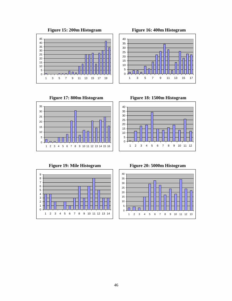
given distance. Illustrated below are the graphs for the marathon, then all of the other

distances in ascending distance order for 2008:

Figure 13: Marathon Histogram Figure 14: 100m Histogram

0

50

100

150

200

250

300

350

400

450

1 2 3 4 5 6 7 8 9 10 11 12 13

0

10

20

30

40

50

60

70

1 2 3 4 5 6 7 8 9 10 11 12 13 14 15 16

46

Figure 15: 200m Histogram Figure 16: 400m Histogram

0

5

10

15

20

25

30

35

40

45

1 3 5 7 9 11 13 15 17 19

0

5

10

15

20

25

30

35

40

1 3 5 7 9 11 13 15 17

Figure 17: 800m Histogram Figure 18: 1500m Histogram

0

5

10

15

20

25

30

35

1 2 3 4 5 6 7 8 9 10 11 12 13 14 15 16

0

5

10

15

20

25

30

35

40

1 2 3 4 5 6 7 8 9 10 11 12

Figure 19: Mile Histogram Figure 20: 5000m Histogram

0

1

2

3

4

5

6

7

8

9

1 2 3 4 5 6 7 8 9 10 11 12 13 14

0

5

10

15

20

25

30

35

40

1 2 3 4 5 6 7 8 9 10 11 12 13

47

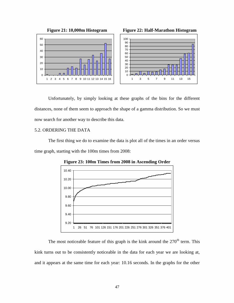
Figure 21: 10,000m Histogram Figure 22: Half-Marathon Histogram

0

10

20

30

40

50

60

1 2 3 4 5 6 7 8 9 10 11 12 13 14 15 16

0

10

20

30

40

50

60

70

80

90

100

1 3 5 7 9 11 13 15

Unfortunately, by simply looking at these graphs of the bins for the different

distances, none of them seem to approach the shape of a gamma distribution. So we must

now search for another way to describe this data.

5.2. ORDERING THE DATA

The first thing we do to examine the data is plot all of the times in an order versus

time graph, starting with the 100m times from 2008:

Figure 23: 100m Times from 2008 in Ascending Order

9.20

9.40

9.60

9.80

10.00

10.20

10.40

1 26 51 76 101 126 151 176 201 226 251 276 301 326 351 376 401

The most noticeable feature of this graph is the kink around the 270th

term. This

kink turns out to be consistently noticeable in the data for each year we are looking at,

and it appears at the same time for each year: 10.16 seconds. In the graphs for the other

48

distances, we are seeing the same occurrence. What this leads us to believe is that there is

a cutoff time at this kink where the data changes distribution. From this point, we decide

to look at only the data prior to this kink, as it appears to follows the same distribution,

and we are not concerned with the slower times from the data set.

5.2.1. KOLMOGOROV – SMIRNOV TEST

Eliminating all of the slower times for each year in the 100m and plotting the

remaining times together, we get:

Figure 24: 100m Times for All Years in Ascending Order

9.40

9.50

9.60

9.70

9.80

9.90

10.00

10.10

10.20

1 20 39 58 77 96 115 134 153 172 191 210 229 248

2008

2007

2006

2005

2004

2003

2002

Notice that in this graph the times for 2008 seem to be faster as a whole than the

times for the other years, indicating that times are getting faster in comparison to the

previous years. However, there also seems to be more data for 2008, which may account

for the difference. We can check to see if the difference is due to an advancement in

performance or a larger data set by using a Kolmogorov - Smirnov test. This test

measures the distances between data points in distributions to test whether or not the

distributions are significantly different from one another. Performing this test for the

49

100m, we find that there is no significant difference between the data sets in the years

2002 – 2007, but the data in the year 2008 is significantly different from the rest. This

tells us that the visible difference is not simply a factor of the larger sample size, and that

times are improving as a whole in 2008.

If we look at the plots of the data in each year for all of the distances, the only

other distance where we can see a difference large enough to warrant a Kolmogorov –

Smirnov test is in the half-marathon, as seen in the graph:

Figure 25: Half-Marathon Times for All Years in Ascending Order

3500

3550

3600

3650

3700

3750

3800

1 31 61 91 121 151 181 211 241 271 301 331 361 391

2008

2007

2006

2005

2004

2003

2002

Running a Kolmogorov - Smirnov test on this data shows that the times from

2008 and 2007 are not significantly different than each other, but together they are

significantly different than the times from the other years, indicating a recent

improvement in half-marathon times.

Also worth noting is that there is no kink in the distribution of the times for this

distance. The only other distance with no prominent kink is the one mile, which also has

the most disperse graph of the times over the years:

50

Figure 26: Mile Times for All Years in Ascending Order

226.00

228.00

230.00

232.00

234.00

236.00

238.00

240.00

242.00

1 6 11 16 21 26 31 36 41 46 51 56 61 66 71 76

2008

2007

2006

2005

2004

2003

2002

5.3. VARIABLES IN DECREASING TIME

Based on the graphs of the data over the years, and the use of the Kolmogorov –

Smirnov test, we can see that some distances are showing the potential to have the world

records fall (100m, half-marathon) while other show that the records seem to be in less

jeopardy of falling (mile, 800m). So what we need to do is figure out a method for

tracking the data over these past years and predicting how low (if at all) the record for a

given distance will fall. Because our data set is limited in how far back we can go, it is

only logical to assume that our extrapolations cannot be made too far into the future. It

would seem impractical to make a prediction about what the world record time will be in

the 100m 150 years from now. So for now, we will be making predictions about the

world record time approximately 10 – 15 years into the future.

5.3.1. IDENTIFYING THE VARIABLES

To measure the how low the records will fall for each distance, we first need to

identify the factors that are driving the times down. Studying the distances over the past

several years, we conclude that there are five main variables that interact to drive the

51

fastest times down. The first variable is what we are terming the “competition ratio”,

which we define to be “the number of times ran in a given year that are measured to be in

the top twenty-five times ever ran up to that point in time”. We can see that as this ratio

approaches one, then the likelihood that a record will be broken will increase due to the

competition increasing. The next variable is the increase / decrease in the competition

ratio from the previous year. This is important because an increase or decrease by some

given amount does not have the same implications for all values of the competition ratio.

The next three variables will not necessarily apply to all distances. We will call

these three variables “incentive”, “phenom”, and “switch”. Incentive is the most complex

of the variables due to the many layers it has. We use the term layers to describe the

many subfactors contributing to the overall incentive effect. Incentive is an increasing

function of societal preference. As an event becomes more popular, there is more

incentive to excel in that particular event. As the societal preference increases, the

monetary rewards will increase. Monetary rewards include prize money, appearance fees,

and endorsement deals. The dichotomy of the incentive effect can be contrasted in the

extremes (100m and marathon) versus the middle distance races (800m, 1500m, mile).

Trends have shown that the middle distance races are much less popular than they once

were in society. In contrast, societal preference for the extremes in the distances are

steadily increasing. The monetary effects of this trend are evident. The top two or three

middle distance runners will receive approximately $50,000 - $75,000 as an appearance

fee to run in a highly promoted professional race [15]. For the marathon, the top ten or

twelve marathoners in the world receive appearance fees of approximately $200,000;

52

Paula Radcliffe, the female world record holder in the marathon and still an active

marathon competitor, commands an appearance fee of $500,000 [11].

On the other extreme, Usain Bolt, world record holder in the men’s 100m and

200m, has a multi-million dollar contract with Puma and other sponsors, and receives

appearance fees of approximately $250,000 per race [17]. It is no coincidence that the

marathon and the 100m are the two events most recently to have the world record broken

(both in 2008).

One of the other variables we are considering is what we are calling the “phenom

effect”. This term can alter by the year, and refers to the presence of a runner who is

currently running in a given event with the capability to lower the world record in that

event within the next approximately 2 – 3 years. We will define the capability to break a

world record as “having ran a time that is within 1% of the world record time in that

year”. This will also account for the current world record holder still actively competing

in an event (as is the case with Usain Bolt in the 100m and 200m).

The final variable we will consider is what we are calling the switch effect. This is

similar to the phenom effect, but it takes into consideration certain athletes who would

normally qualify as phenoms in a given event, but who are not currently competing in

that event. This effect was most recently demonstrated with an athlete named Haile

Gebrselassie, who in 1998 broke the world record for both the 5000m and the 10000m.

Gebrselassie would later switch to the half marathon and then the marathon, both of

which events he successfully lowered the world record, and is currently the world record

holder for the marathon. Of all the variables, this is the most subjective. In order to

qualify for a switch effect, a runner must have publicly declared that they will be making

53

a switch in an event. Also, switches must happen within similar events. The many

distances we are covering can be divided into three categories: sprints, middle distances,

and long distances. The sprints are the 100m, 200m, and 400m; the middle distances are

the 800m, the 1500m, the mile, and sometimes the 5000m; the long distances are

sometimes the 5000m, the 10000m, the half marathon, and the marathon. The reason the

5000m is not strictly defined is because history has seen some athletes make the jump

between the 1500m and the 5000m, but it is a rare occurrence for an athlete to excel in

both events.

5.3.2. QUANTIFYING THE VARIABLES

Now that the variables are defined, we can quantify them. The values we have

found are listed below, with time measured in seconds. The rows highlighted in yellow

indicate that a world record was broken in that year; the rows in orange indicate a world

record was broken twice that year:

Table 23: Variables for 100m

100m

year time comp ratio comp improve incentive phenom switch

2008 9.69 0.44 0.20 1 3 0

2007 9.74 0.24 -0.08 1 2 0

2006 9.77 0.32 0.20 1 2 0

2005 9.77 0.12 -0.04 1 1 0

2004 9.85 0.16 0.16 1 4 0

2003 9.93 0.00 0.00 1 0 0

2002 9.89 0.00 -0.12 1 0 0

54


200m


2008 19.30 0.16 -0.04 1 0 1

2007 19.62 0.20 0.00 1 0 0

2006 19.63 0.20 0.20 1 0 0

2005 19.89 0.00 -0.04 1 0 0

2004 19.79 0.04 0.04 1 0 0

2003 20.01 0.00 -0.04 1 0 0

2002 19.85 0.04 1 0 0


400m


2008 43.75 0.12 0.04 1 0 0

2007 43.45 0.08 0.00 1 1 0

2006 43.62 0.08 0.08 1 1 0

2005 43.93 0.00 0.00 1 0 0

2004 44.00 0.00 0.00 1 0 0

2003 44.57 0.00 0.00 1 0 0

2002 44.45 0.00 1 0 0


800m


2008 102.69 0.00 0.00 0 0 0

2007 103.74 0.00 0.00 0 0 0

2006 103.09 0.00 0.00 0 0 0

2005 103.70 0.00 0.00 0 0 0

2004 103.06 0.00 -0.04 0 0 0

2003 102.52 0.04 -0.04 0 0 0

2002 102.32 0.08 0 0 0


1500m

year time comp ratio comp improve Incentive phenom switch

2008 211.57 0.00 0.00 0 0 0

2007 210.54 0.00 0.00 0 0 0

2006 209.02 0.00 0.00 0 0 0

2005 209.30 0.00 -0.08 0 0 0

2004 207.40 0.08 0.04 0 2 0

2003 208.40 0.04 -0.12 0 0 0

2002 206.89 0.16 0 2 0

55

Table 28: Variables for One Mile

mile


2008 229.38 0.00 -0.04 0 0 0

2007 226.91 0.04 0.04 0 0 0

2006 230.32 0.00 0.00 0 0 0

2005 227.97 0.00 0.00 0 0 0

2004 229.84 0.00 0.00 0 0 0

2003 228.17 0.00 0.00 0 0 0

2002 228.28 0.00 0 0 0


5000m


2008 770.18 0.04 -0.08 0 0 0

2007 769.53 0.12 -0.04 0 0 0

2006 768.09 0.16 0.00 0 0 0

2005 760.18 0.16 0.04 0 1 0

2004 757.35 0.12 -0.16 0 2 0

2003 768.81 0.28 0.28 0 0 0

2002 775.85 0.00 0 0 0

Table 30: Variables for 10,000m

10000m


2008 1585.97 0.04 -0.08 0 1 0

2007 1606.19 0.12 0.00 0 0 0

2006 1595.63 0.12 -0.08 0 0 0

2005 1577.53 0.20 0.08 0 2 0

2004 1580.31 0.12 -0.08 0 1 0

2003 1589.22 0.20 0.00 0 2 0

2002 1609.38 0.20 0 0 0

Table 31: Variables for Half-Marathon

half


2008 3555.00 0.16 -0.48 1 0 0

2007 3513.00 0.64 0.44 1 9 0

2006 3535.00 0.20 0.08 1 5 1

2005 3556.00 0.12 0.08 1 2 0

2004 3611.00 0.04 0.04 1 0 0

2003 3621.00 0.00 -0.16 1 0 0

2002 3585.00 0.16 1 2 0

56

Table 32: Variables for Marathon

marathon


2008 7439.00 0.32 0.24 1 4 0

2007 7466.00 0.08 0.00 1 1 1

2006 7556.00 0.08 -0.04 1 1 0

2005 7580.00 0.12 0.08 1 0 0

2004 7574.00 0.04 0.04 1 0 0

2003 7495.00 0.00 -0.16 1 9 0

2002 7538.00 0.16 1 10 1

We can see that the world records have most recently been broken in the shorter

and longer events, but not in the middle distance events. This is reflected in the low

values for our variables in the middle distance events, and the high values in the shorter

and longer events.

57

CHAPTER 6

FUTURE WORK

6.1. GENERALIZED GAMMA DISTRIBUTION

While we only studied the Gamma distribution using two parameters, there is a

generalized gamma distribution that has three parameters. Though significantly more

complicated than the two parameter version, the generalized gamma may be able to

produce parameter values that will give a chi-square statistic low enough that an

approximation of running times would be acceptable with this distribution.

6.2. SHORTER DISTANCES

Unfortunately, there was not enough time this year to fully examine the effect of

the variables on the fastest yearly times. We have gathered all of the data, and are still in

the process of analyzing the data for trends in the variables to see how accurately we can

model the times. While it is evident that there is a strong correlation between high values

for the variables and fast times for a given year, we need to model the changes in the

variables so we can predict the lower bounds on the times for the years. The variable

“switch” will have to be adjusted yearly, as it would be impossible to predict. However,

estimates on times can be made that take into consideration all scenarios for this variable.

The biggest hurdle in modeling these variables will be in predicting the cycles for

certain distances. The middle distances were once the most popular distances for racing,

but now are the least. The one mile has an advantage in the incentive effect due to it’s’

capability of reacting fastest to the societal preference if the interest is ever reignited. It is

a distance that is ingrained in us from middle school, as it is a commonly used standard

distance for testing one’s physical capabilities. Compare this to the 1500m, just 109

meters shorter in distance, and it is run in the Olympics (the one mile is not). However,

58

the 1500m would take much more time to build up societal preference. All of the

distances would react in a unique way to societal changes, and this is another factor that

will be modeled in the variable estimation in the future.

59

REFERENCES

[1] Abbiss, Chris R. and Paul B Laursen. Sports Med 2008. Describing and

Understanding Pacing Strategies during Athletic Compeition. Vol 38, No. 3.

2008. pp. 239-252.

[2] Behncke, Horst. Journal of Mathematical Biology. A Mathematical Model for the

Force and Energetics in Competitive Running. Vol 31, 1993. pp. 853-878.

[3] Blest, David C. The Statistician. Lower bounds for athletic performance. Vol 45, No.

2. 1996. pp. 243-253.

[4] Chatterjee, Samprit and Sangit. Appl. Statist. New Lamps for Old: An Exploratory

Analysis of Running Times in Olympic Games. Vol 31, No. 1. 1982. pp. 14-22.

[5] Deakin, B. “Estimating Bounds on Athletic Performance”. The Mathematical Gazette.

Vol 51, pp. 100 – 103.

[6] Keller, Joseph B. Physics Today. Optimal Velocity in a Race. Vol 26, No. 9. 1973.

[7] Kennelly, A. “An Approximate Law of Fatigue in Speeds of Racing Animals”.

Proceedings of the American Academy of Arts and Sciences. Vol 61, pp. 487-523.

[8] Lucy, L.B. “Future Progress in the Mile”. IOTA. Vol 1, pp 8 -11.

[9] Mathis, Frank. SIAM Review. The Effect of Fatigue on Running Strategies. Vol. 31,

No. 2 pp. 306-309. June 1989.

[10] Morton, R. Hugh. The Statistician. Statistical effects of lane allocation on times in

running races. Vol 46, No. 1. 1997. pp. 101-104.

[11] Norcross, Dan. “World Marks at Carlsbad Stalled out on Men’s Side”. Union-

Tribune. April 3, 2009.

[12] Schutz, R. W. and McBride, J. P. “The Prediction of Ultimate Track and Field

Performance: Past, Present, Future”. Proceedings of the FISU Conference

Universiade ’83 in Association with the Xth HISPA Congress. pp. 498-515.

[13] Schutz, Robert W. Yuanlong Liu. Statistical Modeling in Track and Field.

[14] Stefani, Raymond T. Chance. Olympic Winning Performances: No Longer Citius,

Altius, Fortius. Vol 13, No. 2. 2000.

60

[15] Steinberg, Dan. “Top Runners Earn Top Dollar on Reputation”. Washington Post.

April 17, 2005. Pg. E04.

[16] http://www.iaaf.org

[17] http://www.singaporeathletics.com

61

BIOGRAPHICAL SKETCH

Kevin Heisler is a senior at Stetson University pursuing a major in Mathematics,

with plans to pursue a career in Actuarial Science after graduation. He was born in

Jupiter, Florida on October 31, 1986. His father, Michael Heisler, is a captain in Palm

Beach County Fire Rescue, and his mother, Belinda Heisler, is a retired Registered

Nurse. Kevin has an identical twin brother, Brian, who also attends Stetson University

and is majoring in Education with a minor in Mathematics.

Kevin has lived in Jupiter his entire life and attended Jupiter Christian School

from kindergarten through twelfth grade. While at Stetson, Kevin ran on the cross

country team for three years. In his spare time Kevin enjoys playing poker, as well as

many other various card games. A self-proclaimed skeptic, he enjoys reading about

conspiracy theories and learning how things work and how they are made. Kevin enjoys

studying numbers and once memorized the first 1,000 digits of pi in four days on a bet

from his roommate.

by kevin heisler - stetson universityefriedma/research/kheisler.pdf · kevin heisler a senior...

Documents