building powerful, predictive scorecards
TRANSCRIPT

white paper
Building Powerful, Predictive ScorecardsAn overview of Scorecard module for FICO® Model Builder
Scorecards are well known as a powerful and palatable predictive modeling
technology with a wide range of business applications. This white paper describes
the technology underlying FICO’s scorecard development platform, the Scorecard
module for FICO® Model Builder. Starting with a brief introduction to scoring and a
discussion of its relationship to statistical modeling, we describe the main elements of
the technology. These include score formulas and score engineering, binning, fitting
objectives and fitting algorithms, characteristic selection, score calibration and score
scaling, performance inference, bootstrap validation, and bagging.
» SummaryMarch 2014
www.fico.com Make every decision countTM

© 2014 Fair Isaac Corporation. All rights reserved. page 2
Building Powerful, Predictive Scorecards
» Introduction . . . . . . . . . . . . . . . . . . . . . . . . . . . . . . . . . . . . . . . 4
» Value Proposition . . . . . . . . . . . . . . . . . . . . . . . . . . . . . . . . . . . . 4
» A Brief Introduction to Scoring . . . . . . . . . . . . . . . . . . . . . . . . . . . . 5
Scoring in the Business Operation . . . . . . . . . . . . . . . . . . . . . . . . . . . . . . . . . . 5
Relationship to Classification and Regression . . . . . . . . . . . . . . . . . . . . . . . . . . . 6
» Scorecard Module Overview . . . . . . . . . . . . . . . . . . . . . . . . . . . . . 7
» Score Formulas . . . . . . . . . . . . . . . . . . . . . . . . . . . . . . . . . . . . . 10
Segmentation . . . . . . . . . . . . . . . . . . . . . . . . . . . . . . . . . . . . . . . . . . . . . .11
Scorecard . . . . . . . . . . . . . . . . . . . . . . . . . . . . . . . . . . . . . . . . . . . . . . . . .12
Characteristics Binning . . . . . . . . . . . . . . . . . . . . . . . . . . . . . . . . . . . . . . . . .13
Ordered Numeric Variables . . . . . . . . . . . . . . . . . . . . . . . . . . . . . . . . . . . . . .13
Categorical or Character String Variables . . . . . . . . . . . . . . . . . . . . . . . . . . . . . .15
Variables of Mixed Type . . . . . . . . . . . . . . . . . . . . . . . . . . . . . . . . . . . . . . . .15
Score Engineering . . . . . . . . . . . . . . . . . . . . . . . . . . . . . . . . . . . . . . . . . . . .16
» Automated Expert Binner . . . . . . . . . . . . . . . . . . . . . . . . . . . . . . 17
Binning Statistics . . . . . . . . . . . . . . . . . . . . . . . . . . . . . . . . . . . . . . . . . . . . .17
Binning Guidelines . . . . . . . . . . . . . . . . . . . . . . . . . . . . . . . . . . . . . . . . . . .18
A Binning Example . . . . . . . . . . . . . . . . . . . . . . . . . . . . . . . . . . . . . . . . . . .20
» Fitting Objective Functions and Algorithms . . . . . . . . . . . . . . . . . . 22
Divergence . . . . . . . . . . . . . . . . . . . . . . . . . . . . . . . . . . . . . . . . . . . . . . . .22
Range Divergence . . . . . . . . . . . . . . . . . . . . . . . . . . . . . . . . . . . . . . . . . . . .23
Bernoulli Likelihood . . . . . . . . . . . . . . . . . . . . . . . . . . . . . . . . . . . . . . . . . . .24
Factored Bernoulli Likelihood . . . . . . . . . . . . . . . . . . . . . . . . . . . . . . . . . . . . .24
Multiple Goal . . . . . . . . . . . . . . . . . . . . . . . . . . . . . . . . . . . . . . . . . . . . . . .24
Least Squares . . . . . . . . . . . . . . . . . . . . . . . . . . . . . . . . . . . . . . . . . . . . . . .25
Penalized Objectives . . . . . . . . . . . . . . . . . . . . . . . . . . . . . . . . . . . . . . . . . .26
Fitting Algorithms . . . . . . . . . . . . . . . . . . . . . . . . . . . . . . . . . . . . . . . . . . . .27
» Automated Characteristic Selection . . . . . . . . . . . . . . . . . . . . . . . 27
» LogOdds to Score Fitting and Scaling . . . . . . . . . . . . . . . . . . . . . . 28
» Performance Inference . . . . . . . . . . . . . . . . . . . . . . . . . . . . . . . . 29
The Problem . . . . . . . . . . . . . . . . . . . . . . . . . . . . . . . . . . . . . . . . . . . . . . .30
Performance Inference Using External Information . . . . . . . . . . . . . . . . . . . . . . .30
table of contents
© 2014 Fair Isaac Corporation. All rights reserved. page 3
Building Powerful, Predictive Scorecards
Performance Inference Using Domain Expertise . . . . . . . . . . . . . . . . . . . . . . . . .31
What Happens in a Parcel Step . . . . . . . . . . . . . . . . . . . . . . . . . . . . . . . . . . . .32
Dual Score Inference and Its Benefits . . . . . . . . . . . . . . . . . . . . . . . . . . . . . . . .32
Summary of Performance Inference . . . . . . . . . . . . . . . . . . . . . . . . . . . . . . . .33
» Bootstrap Validation and Bagging . . . . . . . . . . . . . . . . . . . . . . . . 33
The Problem . . . . . . . . . . . . . . . . . . . . . . . . . . . . . . . . . . . . . . . . . . . . . . .33
Bagging . . . . . . . . . . . . . . . . . . . . . . . . . . . . . . . . . . . . . . . . . . . . . . . . . .36
Summary . . . . . . . . . . . . . . . . . . . . . . . . . . . . . . . . . . . . . . . . . . . . . . . . .36
» Appendix A
Defining Statistical Quantities Used by Scorecard module . . . . . . . . . 37
Principal Sets . . . . . . . . . . . . . . . . . . . . . . . . . . . . . . . . . . . . . . . . . . . . . . .37
Characteristic-Level Statistics for Binary Outcome Problems . . . . . . . . . . . . . . . . .37
Characteristic-Level Statistics for Continuous Outcome Problems . . . . . . . . . . . . . .38
Marginal Contribution . . . . . . . . . . . . . . . . . . . . . . . . . . . . . . . . . . . . . . . . .40
» Appendix B
Performance Evaluation Measures . . . . . . . . . . . . . . . . . . . . . . . . 42
» Appendix C
Scorecards and Multicolinearity . . . . . . . . . . . . . . . . . . . . . . . . . . 44
» References . . . . . . . . . . . . . . . . . . . . . . . . . . . . . . . . . . . . . . . . 46
© 2014 Fair Isaac Corporation. All rights reserved. page 4
Building Powerful, Predictive Scorecards
The purpose of this paper is to provide analytically oriented business users of predictive modeling tools with a description of the Scorecard module for FICO® Model Builder. This should help readers understand the Scorecard module’s business value and exploit its unique modeling options to their fullest advantage. Further, this paper can help analytic reviewers appreciate the strengths and pitfalls of scorecard development, as an aid to ensuring sound modeling practices.
Various generations of scorecard development technology have served FICO and our clients over the decades as the core analytic tools for scorecard development, known historically as “INFORM technology.” For example, the FICO® Score itself is developed using the scorecard technologies described in this paper, and plays a critical role in billions of credit decisions each year. This seminal INFORM technology has evolved over time into a versatile power tool for scorecard development, honed by building tens of thousands of scorecards for the most demanding business clients. Its development has been shaped by the need to develop analytic scorecards of the highest quality while maximizing productivity of analytic staff, and driven by the quest to create new business opportunities based on novel modeling approaches. The latest evolution of INFORM technology incorporates state-of-the-art ideas from statistics, machine learning and data mining in an extensible technological framework, and is readily available to analysts around the globe as the Scorecard module for Model Builder.
FICO’s Scorecard module helps modelers gain insight into their data and the predictive relationships within it, and deal with modeling challenges most likely to be encountered in the practice of score development. With the Scorecard module, modelers can create highly predictive scorecards without sacrificing operational or legal constraints, and deploy these models into operations with ease. The current release of the Scorecard module and the plan for its future enhancements include a rich set of proven, business-adept modeling features.
The remainder of the paper is organized as follows:
• The first section presents the Scorecard module’s value proposition.
• The next section is a brief introduction on scoring in the business operation. We discuss how an important class of business problems can be solved using scoring, and discuss the relationship between scoring, classification and regression. This material may be skipped by those readers with score development experience who are mainly interested in the technical features of the Scorecard module.
The Scorecard module technology has been developed to solve real-world business problems. It is unique in the way it deals with business constraints and data limitations, while maximizing both analysts’ productivity and the predictive power of the developed scorecards. These advantages are achieved through the following set of features:
• Interpretable capture of complex, non-linear relationships based on the scorecard formula.
• Robust modeling even with dirty data, multicollinearity and outliers.
• Penalty parameter and range engineering to ensure model stability.
• Score engineering to address operational and legal constraints.
• Direct incorporation of domain knowledge into the modeling process.
• Ability to directly model numeric, categorical, partially missing and textual predictive variables.
• Amelioration of selection bias and data distortions through performance inference.
» Introduction
» Value Proposition
© 2014 Fair Isaac Corporation. All rights reserved. page 5
Building Powerful, Predictive Scorecards
• Automation of repetitive tasks such as variable binning and score scaling.
• Reason codes to explain the driving forces behind every score calculation and decision.
• Automated documentation of modeling decisions to accelerate analytic validation.
• Rapid deployment of the complete scoring formula.
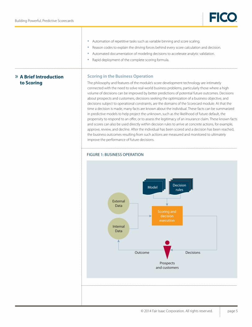
Scoring in the Business OperationThe philosophy and features of the module’s score development technology are intimately connected with the need to solve real-world business problems, particularly those where a high volume of decisions can be improved by better predictions of potential future outcomes. Decisions about prospects and customers, decisions seeking the optimization of a business objective, and decisions subject to operational constraints, are the domains of the Scorecard module. At that the time a decision is made, many facts are known about the individual. These facts can be summarized in predictive models to help project the unknown, such as the likelihood of future default, the propensity to respond to an offer, or to assess the legitimacy of an insurance claim. These known facts and scores can also be used directly within decision rules to arrive at concrete actions, for example, approve, review, and decline. After the individual has been scored and a decision has been reached, the business outcomes resulting from such actions are measured and monitored to ultimately improve the performance of future decisions.
» A Brief Introduction to Scoring
FIGURE 1: BUSINESS OPERATION
InternalData
ExternalData
Scoring anddecision
execution
Prospectsand customers
Model Decisionrules
Outcome Decisions
© 2014 Fair Isaac Corporation. All rights reserved. page 6
Building Powerful, Predictive Scorecards
Examples of data include credit bureau information, purchase histories, web click streams, transactions and demographics. Examples of decision areas include direct marketing, application processing, pricing, account management and transaction fraud detection. Examples of business outcomes include acquisition, revenue, default, profit, response, recovery, attrition and fraud. Examples of business objectives include portfolio profit, balance growth, debt recovered and total fraud dollars saved. Examples of operational constraints include maintenance of a target acceptance rate, total cost or volume of a marketing campaign, requirements to explain adverse decisions to customers and conformance of decision rules with law.
Scoring and decision execution must cope with imperfections of real-world data. Variables can have erroneous or missing values, and score development data samples can be truncated and biased. Data imperfections can result in misleading models and inadequate decisions if no appropriate care is taken.1 Careful injection of domain expertise into the modeling process is often crucial. These insights motivate the requirements for the Scorecard module technology, which make it unique in the market of predictive modeling tools.
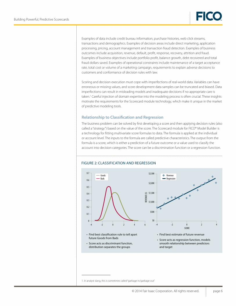
Relationship to Classification and RegressionThe business problem can be solved by first developing a score and then applying decision rules (also called a “strategy”) based on the value of the score. The Scorecard module for FICO® Model Builder is a technology for fitting multivariate score formulas to data. The formula is applied at the individual or account level. The inputs to the formula are called predictive characteristics. The output from the formula is a score, which is either a prediction of a future outcome or a value used to classify the account into decision categories. The score can be a discrimination function or a regression function.
FIGURE 2: CLASSIFICATION AND REGRESSION
GoodsBads
• Find best classification rule to tell apart future Goods from Bads
• Score acts as discriminant function, distribution separates the groups
• Find best estimate of future revenue
• Score acts as regression function, models smooth relationship between predictors and target
0.7
0.6
0.5
0.4
0.3
0.2
0.1
0
-4 -2 0 2 4 6
RevenueRegression
$2,500
$2,000
$1,500
$1,000
$500
$0
-4 -2 0 2 4SCORE
REVE
NUE (
$)
1. In analyst slang, this is sometimes called “garbage in/garbage out.”
© 2014 Fair Isaac Corporation. All rights reserved. page 7
Building Powerful, Predictive Scorecards
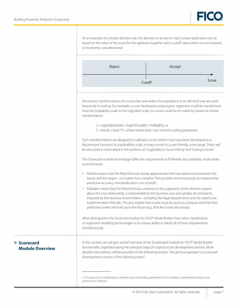
As an example of a simple decision rule, the decision to accept or reject a loan application can be based on the value of the score for this applicant together with a cutoff value (which in turn is based on economic considerations):
Monotonic transformations of a score that rank-orders the population in an identical way are used frequently in scoring. For example, a score developed using logistic regression could be transformed from the probability scale to the log(Odds) scale, or a score could be re-scaled by means of a linear transformation:
S = logOdds(Good) = log(Pr{Good|D} / Pr{Bad|D}), or T = beta0 + beta1*S ; where beta0, beta1 are constant scaling parameters
Such transformations are designed to calibrate a score (which may have been developed as a discriminant function) to a probability scale, or map a score to a user-friendly score range. These will be discussed in more detail in the sections on “Log(Odds)-to-Score Fitting” and “Scaling a Score.”
The Scorecard module technology fulfills the requirements to fit flexible, but palatable, multivariate score formulas:
• Flexible means that the fitted formula closely approximates the true relationship between the inputs and the target—no matter how complex. This provides technical power as measured by predictive accuracy, misclassification cost or profit.
• Palatable means that the fitted formula conforms to the judgments of the domain experts about the true relationship, is interpretable to the business user and satisfies all constraints imposed by the business environment—including the legal requirements and the need to be implementation-friendly. This also implies that scores must be quick to compute and that their predictive power will hold up in the future (e.g., that the scores are robust).
What distinguishes the Scorecard module for FICO® Model Builder from other classification or regression modeling technologies is its unique ability to satisfy all of these requirements simultaneously.
In this section, we will give a brief overview of the Scoreboard module for FICO® Model Builder functionality, organized along the principal steps of a typical score development process. More detailed descriptions will be provided in the following section. The general approach to scorecard development consists of the following steps2:
» Scorecard Module Overview
Reject
Cutoff
Accept
Score
2. This represents a simplification, omitting issues of sampling, generation of new variables, segmentation analysis, and performance inference.

© 2014 Fair Isaac Corporation. All rights reserved. page 8
Building Powerful, Predictive Scorecards
1 . Specify a family of score formulas, which includes binning of predictive variables.
2 . Specify a fitting objective function, which includes specifying a target for prediction.
3 . Specify a variable selection mechanism.
4 . Divide the data into training and test samples.
5 . Let the fitting algorithm optimize the fitting objective function on the training sample.
6 . Evaluate the merits of the fitted score based on the test sample.
7 . Modify the above specifications until satisfied with predictive power and palatability of the score.
8 . Deploy the model.
The Scorecard module’s choices for these steps are as follows:
1. The Scorecard module’s family of score formulas is based on the Generalized Additive Model (GAM) [See Reference 1]. This model class captures nonlinear relationships between predictive variables and the score. The structure of the Scorecard module’s GAM score formula requires the generation of predictive characteristics prior to model training, through a process called “binning.”3 The score arises as a weighted sum of features derived from these characteristics. The simplest and most frequently used representation of the Scorecard module’s score formula is the discrete scorecard, where the features are indicator variables for the bins4 and the feature weights are score weights. In addition to the GAM part of the score formula, it is also possible to model interactions.5 A unique feature of the Scorecard module—not found in off-the-shelf GAM tools—is the capability to constrain the score formulas to exhibit particular, desirable patterns or shapes. Such “score engineering” constraints are very useful to make a scorecard more interpretable, adhere to legal or operational constraints, and instill domain knowledge into a score development—as well as to overcome data problems and increase robustness of the score.
2. The Fitting Objective Function (FOF) guides the search for the “best” model or scorecard, which optimizes the FOF on the training sample. The Scorecard module allows for flexible choices for the FOF, offering Divergence, Range Divergence, Bernoulli Likelihood, Least Squares and Multiple Goal.6 With the exception of Least Squares, these objectives have in common that a binary-valued target variable needs to be defined.7 In the case of Multiple Goal, a secondary target variable also needs to be defined. In the case of Least Squares, the target is a continuous numeric variable. In all cases, a penalty term for large score weights can be added to the primary fitting objective to ensure solution stability.8 Range Divergence is used to amplify or reduce the influence of certain predictive characteristics in a scorecard, while controlling for possible loss of the primary fitting objective, Divergence. This offers another powerful engineering mechanism to improve
3. Binning is the analytic activity to partition the value ranges of predictive variables into mutually exclusive and exhaustive sets, called “bins.” The Scorecard module’s binner activity offers an automated approach to this otherwise tedious manual process. A variable combined with a binning scheme is called a “characteristic.”
4. The value of the indicator variable for a given bin is 1 if the value of the binned variable falls into that bin and 0 otherwise.
5. Technically, an interaction exists if the effect of one predictive variable on the score depends on the value of another predictive variable. Various ways for capturing interactions exist: (i) by generating derived variables from the raw data set variables (such as product-, ratio-, and rules-based variables), (ii) by generating “crosses” between characteristics (which present a bivariate generalization of the characteristics concept), and (iii) by developing segmented scorecard trees (where each leaf of the tree represents a specific sub-population, which is modeled by its own dedicated scorecard). The construction of the segmented scorecard tree is discussed in the FICO white paper Using Segmented Models for Better Decisions [2].
6. See Appendix A on “Scorecard module statistical measures” for definitions.
7. This is handled in the Scorecard module through the concept of “Principal Sets” (See Appendix A).
8. The penalty term is a regularization technique, related to the Bayesian statistical concept of “shrinkage estimators,” which introduce a small amount of bias on the model estimates in order to reduce variability of these estimates substantially.
© 2014 Fair Isaac Corporation. All rights reserved. page 9
Building Powerful, Predictive Scorecards
scorecard’s business utility or robustness.9 A scorecard fitted with Bernoulli Likelihood is a close cousin to a technique known as “dummy variable logistic regression,” with the added value that the model can be developed as a palatable, engineered scorecard. Similarly, the Least Squares scorecard is a close cousin to dummy variable linear regression, with the added benefits of score engineering and palatability. The Multiple Goal objective function allows for the development of a scorecard with good rank-ordering properties with respect to a primary and a secondary target.10 The inevitable tradeoff between the competing targets can be directly controlled by the analyst.
3. Automated characteristic selection is sometimes used to increase score development productivity, especially when there are many candidate characteristics for possible inclusion in the scorecard.11 The Scorecard module’s automated characteristic selection criteria are based on the unique concept of Marginal Contribution12 and offer unique capabilities to take user preferences for, and dependencies between, characteristics into account.
4. The scorecard is fitted on a training sample. The Scorecard module allows specifying a test sample, and supports comparative views of training and test samples. Test sample performance helps in judging the statistical credibility of the fitted model, provides a defense against over-fitting to the peculiarities of a training sample, and helps in developing robust scorecards that perform well on new data. In situations where the development sample is too small to allow for reliable validation using a training/test split, bootstrap validation is available to help. This is a statistically sound validation technique, which uses the entire sample for fitting the model, so no information is lost for model development. The algorithm is computationally intensive and we recommended it primarily for small sample situations. See Bootstrap Validation and Bagging section for more information.
5. The fitting algorithm solves for the optimal set of score weights, such that the fitting objective function is maximized (or minimized) subject to possible score engineering constraints. The Scorecard module’s fitting algorithms are based on industrial-strength quadratic and nonlinear programming technology and are designed for efficient and reliable fitting of large scorecards.13 At the same time, they allow for score engineering constraints and automated characteristic selection.
6. The business benefits of a scorecard can be evaluated in terms of the value achieved on some Business Objective Functions (BOF). The BOF can be different from the FOFs as discussed under item 2. As an example, a FOF used in a score development could be penalized Range Divergence, while the BOF reported to the business user could be misclassification cost, or ROC Area.14 Other determinants of the benefit of a scorecard are its interpretability, ease of implementation, and adherence to legal and business constraints.
7. The Scorecard module for FICO® Model Builder empowers analysts to develop business-appropriate scorecards by offering a versatile choice set for score formula, score engineering constraints, and objective functions. Analysts frequently develop dozens of scorecards based on alternative specifications before achieving overall satisfaction with a model. The Scorecard module supports these exploratory modeling iterations through its model management, automatic versioning and reporting capabilities.
9. For example, Range Divergence can address legal or marketing constraints on adverse action reporting (reasons provided to consumers whose loan applications were turned down).
10. For example, for a marketing offer to be most profitable, you want a high response rate and high revenue from the responders. Since some prospects that are the best responders may be among the first to attrite or default, you want to identify and target customers most likely to respond (primary target) and stay on to generate revenue (secondary target).
11. Characteristic libraries and FICO’s Data Spiders™ technology can easily generate thousands of candidate characteristics. Normally, these are filtered down prior to training the first scorecard, but a larger set may still exist even after such filtering.
12. See Appendix A on “Scorecard module statistical measures” for definitions.
13. What constitutes “large” is domain-dependent, and is a function of the model size, not the data size. Larger scorecards may include 300 or more score weights, although such models are less frequently found.
14. See Appendix A for definitions.

© 2014 Fair Isaac Corporation. All rights reserved. page 10
Building Powerful, Predictive Scorecards
8. The module’s scorecards are easy to deploy to a number of applications, without any manual recoding of the model, thanks to the FICO decision management architecture.
The following chapters discuss in more detail the main elements of FICO’s score development technology:
• Score formulas
• Automated Expert Binner
• Fitting objective functions
• Fitting algorithms
• Characteristic selection
There are many technologies for fitting regression or discriminant functions for prediction and classification. Some technologies, including neural networks, regression and classification trees, or support vector machines, belong to the class of “universal approximators.” These can approximate just about any relationship between a set of predictive variables and the score, no matter how complicated. The enormous flexibility of these technologies offers high technical power. However, this strength is sometimes accompanied by a lack of model interpretability. Interpretability can be a critical factor in a number of important business modeling applications—including credit risk scoring and insurance underwriting—which require model interpretability, as well as the ability of the model developer and user to instill domain knowledge into the modeling process. The Scorecard module’s benefit of simultaneously maximizing technical power as well as interpretability is based on the Generalized Additive Model (GAM) structure of the FICO® Model Builder family of score formulas. This structure provides palatability by combining universal approximator capability with score engineering constraints.
This description of the scorecard system begins at the top level, which is a segmented scorecard tree. The next level describes the single scorecard. One level further below the scorecard is a description of the scorecard characteristic, which forms the basis of the module’s family of score formulas.
» Score Formulas
© 2014 Fair Isaac Corporation. All rights reserved. page 11
Building Powerful, Predictive Scorecards
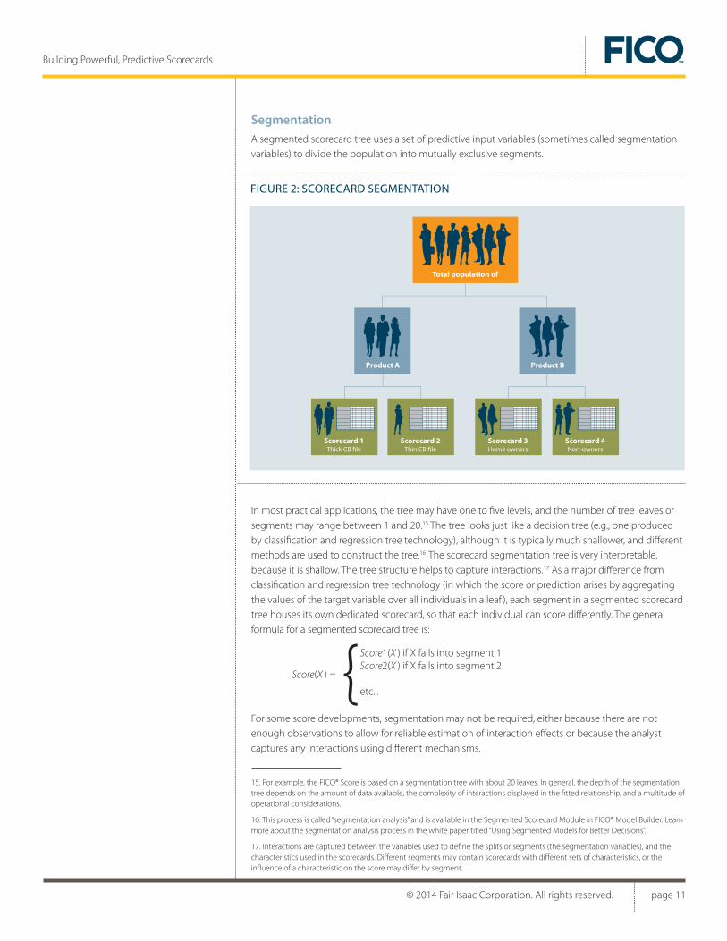
SegmentationA segmented scorecard tree uses a set of predictive input variables (sometimes called segmentation variables) to divide the population into mutually exclusive segments.
In most practical applications, the tree may have one to five levels, and the number of tree leaves or segments may range between 1 and 20.15 The tree looks just like a decision tree (e.g., one produced by classification and regression tree technology), although it is typically much shallower, and different methods are used to construct the tree.16 The scorecard segmentation tree is very interpretable,because it is shallow. The tree structure helps to capture interactions.17 As a major difference fromclassification and regression tree technology (in which the score or prediction arises by aggregating the values of the target variable over all individuals in a leaf ), each segment in a segmented scorecard tree houses its own dedicated scorecard, so that each individual can score differently. The general formula for a segmented scorecard tree is:
For some score developments, segmentation may not be required, either because there are not enough observations to allow for reliable estimation of interaction effects or because the analyst captures any interactions using different mechanisms.
15. For example, the FICO® Score is based on a segmentation tree with about 20 leaves. In general, the depth of the segmentation tree depends on the amount of data available, the complexity of interactions displayed in the fitted relationship, and a multitude of operational considerations.
16. This process is called “segmentation analysis” and is available in the Segmented Scorecard Module in FICO® Model Builder. Learn more about the segmentation analysis process in the white paper titled “Using Segmented Models for Better Decisions”.
17. Interactions are captured between the variables used to define the splits or segments (the segmentation variables), and the characteristics used in the scorecards. Different segments may contain scorecards with different sets of characteristics, or the influence of a characteristic on the score may differ by segment.
FIGURE 2: SCORECARD SEGMENTATION
Scorecard 4Non-owners
Scorecard 3Home owners
Scorecard 2Thin CB file
Total population of
Product A Product B
Scorecard 1Thick CB file
Score(X ) =
Score1(X ) if X falls into segment 1Score2(X ) if X falls into segment 2
etc...

© 2014 Fair Isaac Corporation. All rights reserved. page 12
Building Powerful, Predictive Scorecards
ScorecardThe scorecards in the segments are developed independently in the Scorecard module, one at a time, for each segment of the scorecard tree. Here is an example of a scorecard:
The mathematical formula for an additive scorecard is:
18. It is also possible to add “cross characteristics” to a scorecard, which is not shown here. Crosses capture the combined impact of two variables on the score, which provides another mechanism to capture interactions.
Characteristic J Bin K Description Score Weight
Age of account2
Debt ratio3
1
2
1
2
3
1
2
3
0
1
2 or more
Below 1 year
1-2 year
0-30
30-50
50-70
etc.
etc.
20
10
15
10
10
5
5
5
Number of late payments in last 9 months1
FIGURE 4: MINIATURE EXAMPLE OF A SCORECARD
Simulated figures for illustrative purpose only
The predictive characteristics and their bin descriptions are listed, along with the respective score weights. Given an account or individual who occupies a particular combination of characteristic bins, the score weights for these bins are added up to result in the total score value. This renders the above example scorecard a Generalized Additive Model.18
( )+= ∑=
Score
S0 = Intercept (only for Bernoulli Likelihood objective function)
c1,
c2,
..., cp = Scorecard characteristics
H(.)= Characteristic score
S1,S
2,...,S
q = Score weights associated with the bins of a characteristics
X1,X
2,...,X
q= Dummy indicator variables for the bins of a characteristics
1
0
p
jjj cHS
= 0
if Age of Account is below 1 year
else
1 e.g. ix
( )= ∑=1
q
iii cxS
{
© 2014 Fair Isaac Corporation. All rights reserved. page 13
Building Powerful, Predictive Scorecards
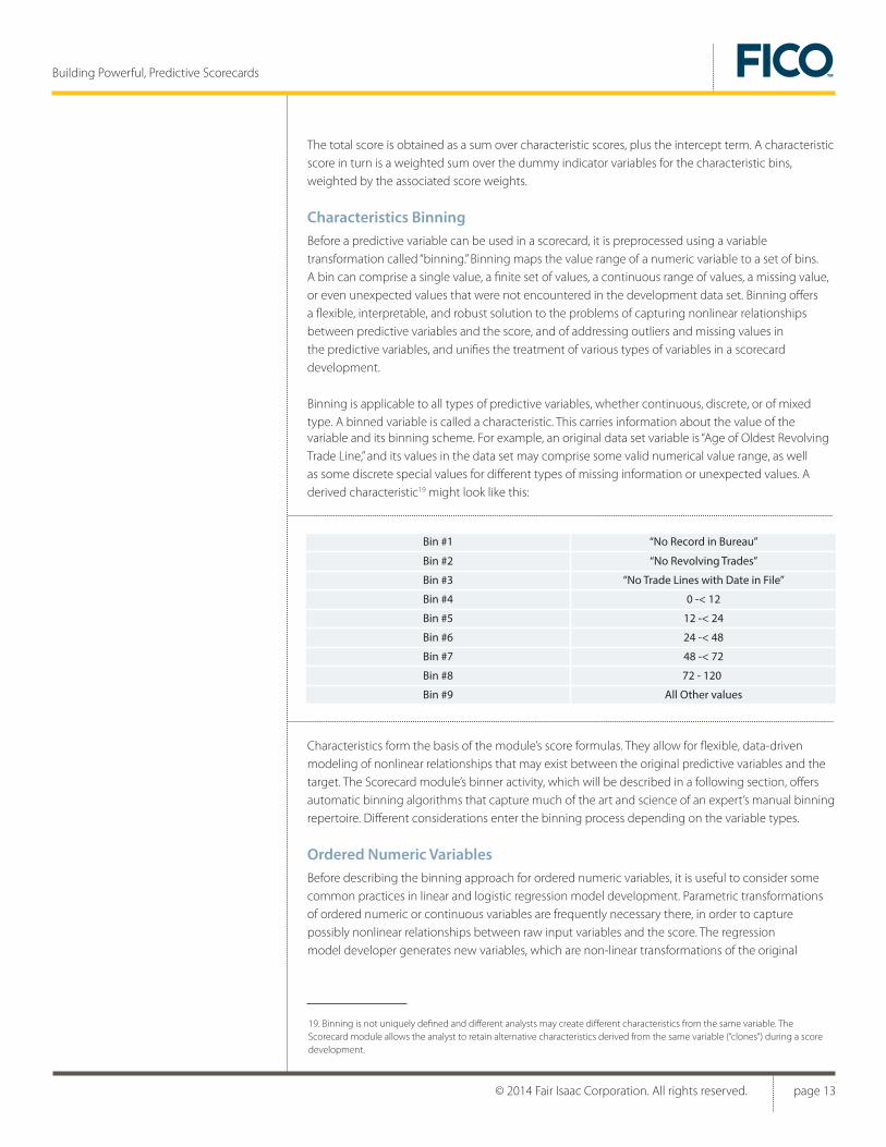
variable and its binning scheme. For example, an original data set variable is “Age of Oldest Revolving Trade Line,” and its values in the data set may comprise some valid numerical value range, as well as some discrete special values for different types of missing information or unexpected values. A derived characteristic19 might look like this:
Characteristics form the basis of the module’s score formulas. They allow for flexible, data-driven modeling of nonlinear relationships that may exist between the original predictive variables and the target. The Scorecard module’s binner activity, which will be described in a following section, offers automatic binning algorithms that capture much of the art and science of an expert’s manual binning repertoire. Different considerations enter the binning process depending on the variable types.
Ordered Numeric VariablesBefore describing the binning approach for ordered numeric variables, it is useful to consider some common practices in linear and logistic regression model development. Parametric transformations of ordered numeric or continuous variables are frequently necessary there, in order to capture possibly nonlinear relationships between raw input variables and the score. The regression model developer generates new variables, which are non-linear transformations of the original
The total score is obtained as a sum over characteristic scores, plus the intercept term. A characteristic score in turn is a weighted sum over the dummy indicator variables for the characteristic bins, weighted by the associated score weights.
Characteristics BinningBefore a predictive variable can be used in a scorecard, it is preprocessed using a variable transformation called “binning.” Binning maps the value range of a numeric variable to a set of bins. A bin can comprise a single value, a finite set of values, a continuous range of values, a missing value, or even unexpected values that were not encountered in the development data set. Binning offers a flexible, interpretable, and robust solution to the problems of capturing nonlinear relationships between predictive variables and the score, and of addressing outliers and missing values in the predictive variables, and unifies the treatment of various types of variables in a scorecard development.
Binning is applicable to all types of predictive variables, whether continuous, discrete, or of mixed type. A binned variable is called a characteristic. This carries information about the value of the
19. Binning is not uniquely defined and different analysts may create different characteristics from the same variable. The Scorecard module allows the analyst to retain alternative characteristics derived from the same variable (“clones”) during a score development.
Bin #1
Bin #2
Bin #5
Bin #6
Bin #3
Bin #9
72 - 120Bin #8
Bin #7
“No Record in Bureau”
“No Revolving Trades”
“No Trade Lines with Date in File”
12 -< 24
24 -< 48
All Other values
48 -< 72
0 -< 12Bin #4
© 2014 Fair Isaac Corporation. All rights reserved. page 14
Building Powerful, Predictive Scorecards
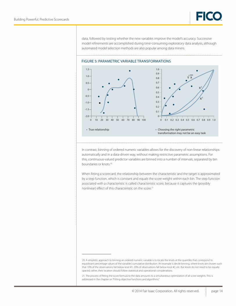
data, followed by testing whether the new variables improve the model’s accuracy. Successive model refinements are accomplished during time-consuming exploratory data analysis, although automated model selection methods are also popular among data miners.
In contrast, binning of ordered numeric variables allows for the discovery of non-linear relationships automatically and in a data-driven way, without making restrictive parametric assumptions. For this, continuous-valued predictor variables are binned into a number of intervals, separated by bin boundaries or knots.20
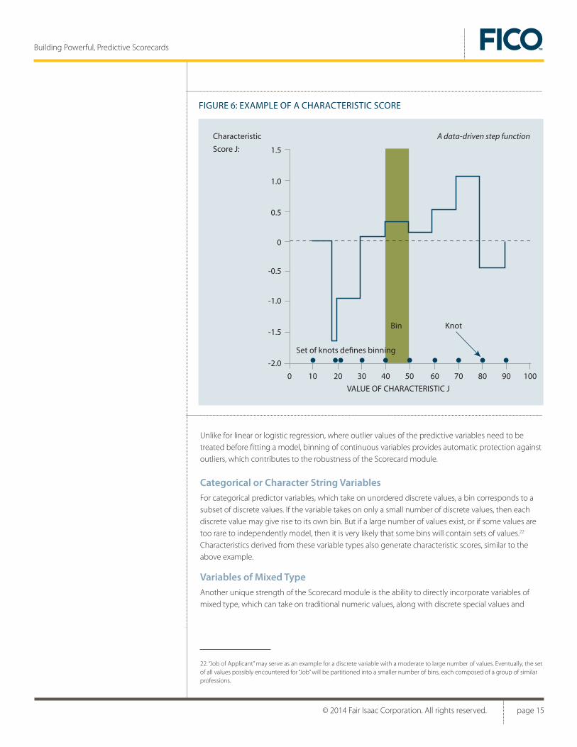
When fitting a scorecard, the relationship between the characteristic and the target is approximated by a step function, which is constant and equals the score weight within each bin. The step function associated with a characteristic is called characteristic score, because it captures the (possibly nonlinear) effect of this characteristic on the score.21
FIGURE 5: PARAMETRIC VARIABLE TRANSFORMATIONS
1.0
0.9
0.8
0.7
0.6
0.5
0.4
0.3
0.1
0.2
0
0 0.2 0.30.1 0.4 0.5 0.6 0.7 0.8 0.9 1.0
1.5
1.0
0.5
0
-0.5
-1.0
-1.5
-2.0
0 20 3010 40 50 60 70 80 90 100
• True relationship • Choosing the right parametric transformation may not be an easy task
√ x
x2
x3
20. A simplistic approach to binning an ordered numeric variable is to locate the knots at the quantiles that correspond to equidistant percentage values of the variables’ cumulative distribution. An example is decile binning, where knots are chosen such that 10% of the observations fall below knot #1, 20% of observations fall below knot #2, etc. But knots do not need to be equally spaced, rather, their location should follow statistical and operational considerations.
21. The process of fitting the score formula to the data amounts to a simultaneous optimization of all score weights. This is addressed in the chapter on “Fitting objective functions and algorithms.”
© 2014 Fair Isaac Corporation. All rights reserved. page 15
Building Powerful, Predictive Scorecards
Unlike for linear or logistic regression, where outlier values of the predictive variables need to be treated before fitting a model, binning of continuous variables provides automatic protection against outliers, which contributes to the robustness of the Scorecard module.
Categorical or Character String VariablesFor categorical predictor variables, which take on unordered discrete values, a bin corresponds to a subset of discrete values. If the variable takes on only a small number of discrete values, then each discrete value may give rise to its own bin. But if a large number of values exist, or if some values are too rare to independently model, then it is very likely that some bins will contain sets of values.22 Characteristics derived from these variable types also generate characteristic scores, similar to the above example.
Variables of Mixed TypeAnother unique strength of the Scorecard module is the ability to directly incorporate variables of mixed type, which can take on traditional numeric values, along with discrete special values and
22. “Job of Applicant” may serve as an example for a discrete variable with a moderate to large number of values. Eventually, the set of all values possibly encountered for “Job” will be partitioned into a smaller number of bins, each composed of a group of similar professions.
FIGURE 6: EXAMPLE OF A CHARACTERISTIC SCORE
1.5
1.0
0.5
0
-0.5
-1.0
-1.5
-2.0
0 20 3010 40 50 60 70 80 90 100
Set of knots defines binning
Bin Knot
Characteristic A data-driven step function
Score J:
VALUE OF CHARACTERISTIC J

© 2014 Fair Isaac Corporation. All rights reserved. page 16
Building Powerful, Predictive Scorecards
missing values. The variable discussed earlier, “Age of Oldest Revolving Trade Line”, illustrates this mixed-type case. Characteristics derived from these variable types also generate characteristic scores.
Score EngineeringThe high degree of flexibility of the module’s score formula is a boon for complicated non-linear curve fitting applications. But scorecard development is often constrained by data problems and business considerations unrelated to the data. In these cases, the Scorecard module empowers the analyst to limit the flexibility of the score formula by constraining or “score engineering” it in several important ways. Score engineering allows the user to impose constraints on the score formula to enhance palatability, meet legal requirements, guard against over-fitting, ensure robustness for future use, and adjust for known sample biases.
The Scorecard module offers a variety of score engineering constraints, which can be applied to individual characteristic scores and also across multiple characteristics. Score engineering capabilities include:
• Centering
• Pattern constraints
• In-weighting
• No-inform or zeroing
• Cross-constraints between different components of the model
• Range engineering
In the case of the Bernoulli Likelihood objective, the intercept can also be in-weighted. The score engineering constraints put restrictions on the form of the score formula or scorecard weights. The Scorecard module’s model fitting algorithm is, in fact, a mathematical programming solver: It finds the scorecard weights which optimize the fitting objective function while satisfying these constraints.
ExampleScore engineering includes advanced options to constrain the shape of the characteristic score curve for palatability, score performance and robustness. For example, palatability of the model may demand that the characteristic score is non-decreasing across the full numeric range of the variable (or perhaps across a specific interval). This is easily guaranteed by applying pattern constraints to the bins of the characteristic.
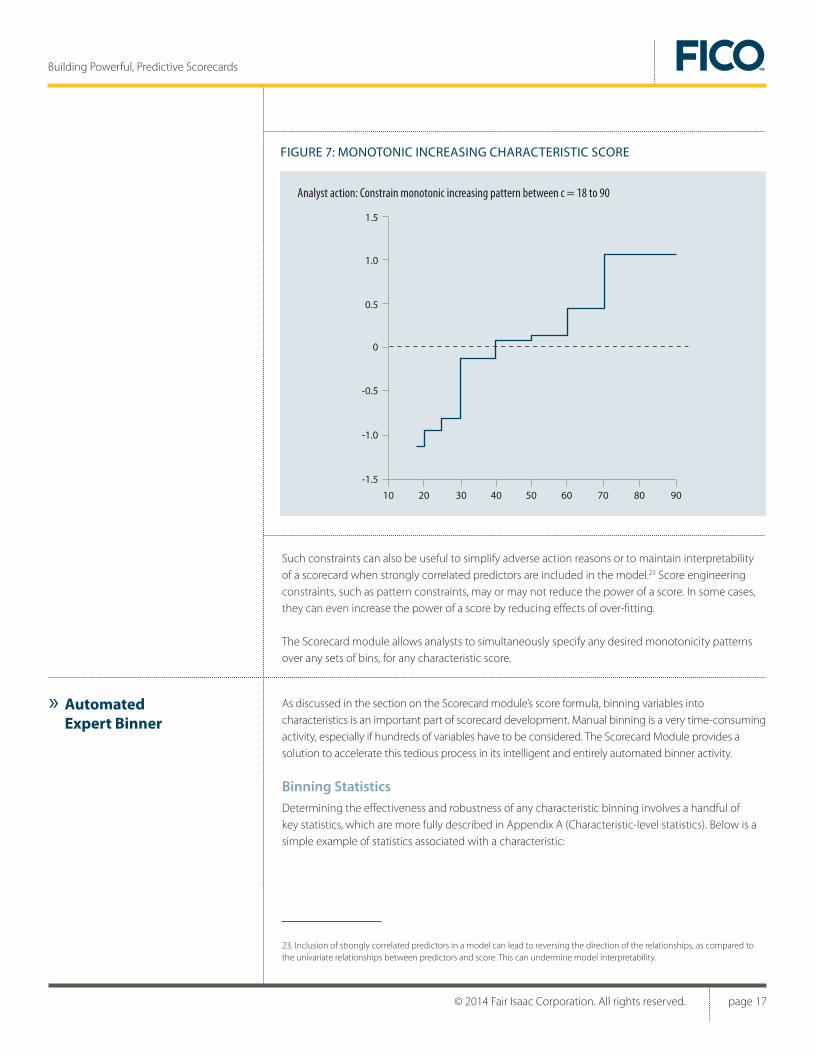
One important application of this example arises from legal requirements in the US (Equal Credit Opportunity Act, Regulation B). Law demands that for a credit application scorecard, elderly applicants must not be assigned lower score weights. If the training data contradict this pattern (as shown in Figure 6) then the characteristic score for “Applicant Age” could be constrained to enforce a monotonically increasing pattern, as seen in Figure 7.
© 2014 Fair Isaac Corporation. All rights reserved. page 17
Building Powerful, Predictive Scorecards
Such constraints can also be useful to simplify adverse action reasons or to maintain interpretability of a scorecard when strongly correlated predictors are included in the model.23 Score engineering constraints, such as pattern constraints, may or may not reduce the power of a score. In some cases, they can even increase the power of a score by reducing effects of over-fitting.
The Scorecard module allows analysts to simultaneously specify any desired monotonicity patterns over any sets of bins, for any characteristic score.
As discussed in the section on the Scorecard module’s score formula, binning variables into characteristics is an important part of scorecard development. Manual binning is a very time-consuming activity, especially if hundreds of variables have to be considered. The Scorecard Module provides a solution to accelerate this tedious process in its intelligent and entirely automated binner activity.
Binning StatisticsDetermining the effectiveness and robustness of any characteristic binning involves a handful of key statistics, which are more fully described in Appendix A (Characteristic-level statistics). Below is a simple example of statistics associated with a characteristic:
23. Inclusion of strongly correlated predictors in a model can lead to reversing the direction of the relationships, as compared to the univariate relationships between predictors and score. This can undermine model interpretability.
FIGURE 7: MONOTONIC INCREASING CHARACTERISTIC SCORE
1.5
1.0
0.5
0
-0.5
-1.0
-1.5
10 3020 40 50 60 70 80 90
Analyst action: Constrain monotonic increasing pattern between c = 18 to 90
» Automated Expert Binner

© 2014 Fair Isaac Corporation. All rights reserved. page 18
Building Powerful, Predictive Scorecards
Where:
The WOE statistic clearly shows that observations falling into the “Low” bin have a somewhat neutral risk (in line with the population average, with a WOE very close to 0), the “Medium” bin indicates better risk (WOE notably higher than 0), and the “High” bin indicates worse risk (sharply lower than 0). Judging from its IV value of 0.1151, is this a useful predictive characteristic? The answer depends on the difficulty of the prediction problem, which can vary from one score development to another. If many characteristics exist, it may be more interesting to rank-order them according to their IVs and to initially pay more attention to those with higher IV values.
Experienced scorecard developers also compare the observed WOE patterns with their expectations and domain knowledge. If the WOE pattern contradicts expectations, then this may indicate a data problem and trigger further research. If the WOE pattern matches expectations, then this characteristic may become a favorite candidate characteristic for the scorecard.
The above statistics are also important to decide how a variable should be binned. For example, one may attempt to combine the Low and Medium bins of the above characteristic into a single bin and simulate the resulting loss in IV for the new characteristic. If the loss is small enough, one might want to use the new characteristic as a candidate for a less complex scorecard.
Seasoned scorecard developers tend to spend considerable time reviewing and fine-tuning binning and characteristic generation. This is not surprising, because binning generates first insights into predictive data relationships. One may be able to confirm or question the meaning of certain variables and sometimes discover data problems.
Binning GuidelinesBinning can be seen as an exploratory data analysis activity and also as a first step in developing a predictive scorecard. It would be very ambitious to provide a general “recipe” for how best to bin a given variable. This depends on the context, including the goals of binning and the details of the scorecard development specifications.
Description nL nR fL fR WOE IVcontrib
1
2
3
Low
Medium
High
1350
2430
897
Total 4677
19
27
23
69
28.9
52.0
19.2
100
27.5
39.1
33.3
100 IV = 0.1151
0.0497
0.2851
-0.5506
0.0007
0.0368
0.0776
Bin #
nL / R
: Observation counts from Left / Right principal set
f L / R
: Corresponding observation percentages
WOE : Weight of Evidence
IVcontrib : Bin contribution to Information Value
IV : Information Value

© 2014 Fair Isaac Corporation. All rights reserved. page 19
Building Powerful, Predictive Scorecards
However, useful guidelines have emerged through many years of practical experience. Overall, characteristics should be generated in such a way that they are both predictive and interpretable. This includes a number of considerations and tradeoffs:
• Make the bins wide enough to obtain a sufficient amount of “smoothing” or noise reduction for estimation of WOE statistics. An important requirement is that the bins contain a sufficient number of observations from both Principal Sets (see Appendix for a definition of “Principal Sets”).
• Make the bins narrow enough to capture the signal—the underlying relationship between predictive variable and score. Too coarse a binning may incur a loss of information about the target, leading to a weaker model.
• In the case of numeric variables, scorecard developers may want to choose knots between bins that are located at convenient, business-appropriate or “nice” values.
• Some analysts like to define bins for certain numeric variables in a way that the WOE patterns follow an anticipated monotonic relationship.
• In the case of discrete variables with many values, coarse bins could be chosen to encompass qualitatively similar values, which may require domain expertise.
There are undoubtedly more tricks of the trade than we have listed here. Since successful binning remains a combination of art and science, analyst experience and preferences matter. Often it is not obvious how to define bins, so that alternative solutions should be compared. In projects where there are many potential predictive variables, a considerable amount of time will thus be spent exploring bin alternatives.
The Scorecard module’s advanced binner activity automates the tedious aspects of binning. At the same time, it allows the analyst to specify options and preferences for binning characteristics in uniquely flexible ways. Finally, the Scorecard module provides an efficient and visual interactive binner, which combines total manual control, immediate feedback and powerful editing functions to allow the analyst to refine solutions produced by the automated binner.

© 2014 Fair Isaac Corporation. All rights reserved. page 20
Building Powerful, Predictive Scorecards
A Binning ExampleIt is easiest to describe the workings of the automated expert binner by means of an example. Consider the numeric variable “Previous Payment Amount.” It has a distribution in the development sample, which can be displayed as a histogram of counts:
The most common recent payment amounts are between $2,000 and $4,000. There are, however, a long tail of larger payment amounts that are well above this range. In addition, there are two unusual values (-998 and -999). Upon further enquiry, the analyst learns that -998 carries a special meaning—a -998 value may mean that the account just opened so no payment has yet been made. The analyst also learns that -999 means that the account was closed and the last payment amount is now unavailable in the dataset.
In lieu of domain knowledge, a simplistic approach to binning might be to locate the knots at quantile values for equal bin percentages. In the histogram above, we indicate the quantile binning by the horizontal dotted lines, which divide the payment amounts into five quantiles, with 20% of the observations falling into each bin. A scorecard developer may want to improve on this binning for several reasons, including:
• Distinction between outstanding and normal values has been lost.
• Bin breaks or knows are located at “odd” values, such as $2998, $7856, etc., which may not appeal to the psyche of the scorecard user.
• Intuitively, bins could be chosen wider where the relationship between predictive variable and score can be expected to be flat and narrower where the relationship rapidly changes. This requires comparing alternative binnings. Quantile binning completely ignores the distribution of the target variable, which may lead to significant information loss.
FIGURE 8: LAST PAYMENT AMOUNT HISTOGRAM
9,000
8,000
7,000
6,000
5,000
4,000
3,000
2,000
1,000
0-999
-998$1,000 $3,000 $6,000 $8,000 $10,000 $12,000 $14,000
LAST PAYMENT AMOUNT ($)
FREQ
UEN
CY
© 2014 Fair Isaac Corporation. All rights reserved. page 21
Building Powerful, Predictive Scorecards
The automated expert binning activity overcomes these limitations through its advanced binning features:
• User can specify preferences for bin breaks and outstanding values (templates exist for various variable scales and conventions for outstanding values).
• Automated expert binning handles special values which can denote different types of missing information.
• Automated expert binning controls potential IV loss due to binning, based on user-defined parameters.
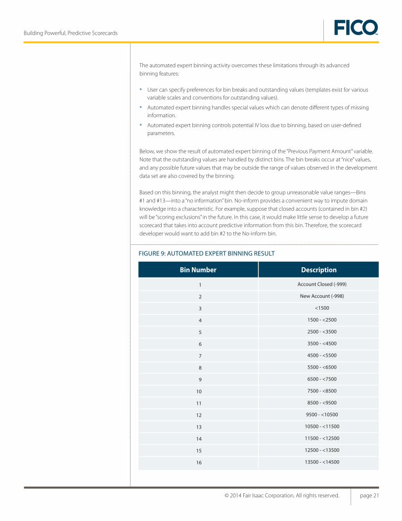
Below, we show the result of automated expert binning of the “Previous Payment Amount” variable. Note that the outstanding values are handled by distinct bins. The bin breaks occur at “nice” values, and any possible future values that may be outside the range of values observed in the development data set are also covered by the binning.
Based on this binning, the analyst might then decide to group unreasonable value ranges—Bins #1 and #13—into a “no information” bin. No-inform provides a convenient way to impute domain knowledge into a characteristic. For example, suppose that closed accounts (contained in bin #2) will be “scoring exclusions” in the future. In this case, it would make little sense to develop a future scorecard that takes into account predictive information from this bin. Therefore, the scorecard developer would want to add bin #2 to the No-inform bin.
FIGURE 9: AUTOMATED EXPERT BINNING RESULT
Bin Number Description
1
2
3
4
5
6
7
8
9
10
11
12
13
14
15
16
Account Closed (-999)
New Account (-998)
<1500
1500 - <2500
2500 - <3500
3500 - <4500
4500 - <5500
5500 - <6500
6500 - <7500
7500 - <8500
8500 - <9500
9500 - <10500
10500 - <11500
11500 - <12500
12500 - <13500
13500 - <14500

© 2014 Fair Isaac Corporation. All rights reserved. page 22
Building Powerful, Predictive Scorecards
Assuming that a candidate set of binned characteristics has been created, and possible score engineering constraints have been applied to the score formula, the score formula can now be fitted to the data. The actual fitting process is governed by the fitting objective function and characteristic selection considerations, which we will describe in turn.
We have presented only the tip of the iceberg of possible binning considerations. The Scorecard module’s automated expert binner offers an even wider range of options, including similarity—and pattern—based coarse binning stages. A “rounding type” can also be defined for each predictive characteristic, which holds standard and customizable business rules that interact with the count statistics to create the most informative and easy-to-interpret binning results.
The current release of the Scorecard module for FICO® Model Builder offers five objective functions:
• (Penalized) Divergence
• (Penalized) Range Divergence
• (Penalized) Bernoulli Likelihood
• (Penalized) Multiple Goal
• (Penalized) Least Squares
With the notable exception of Least Squares, these objective functions require that the business outcome has been dichotomized into a binary target variable for classification, by defining Left and Right Principal Sets (in short, L and R). See Appendix A for a more in-depth discussion of these sets. Multiple Goal also requires a secondary, typically continuous-valued, target variable.
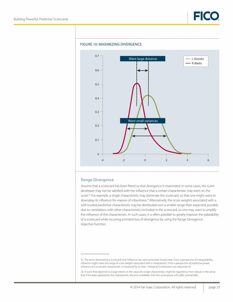
DivergenceDivergence of a score is a statistical measure of score power defined on moments of the score distribution. It plays a central role in the theory of discriminant analysis, where the goal is to find an axis in the multidimensional space of predictors along which two groups can best be discriminated. The intuitive objective associated with a good discrimination capability of the score is to separate the score distributions for L and R as much as possible. This requires a large distance between the conditional means, along with small variance around these means, and thus, a large value of divergence. Refer to Appendix A for a mathematical definition of divergence.
Scores developed to maximize divergence possess excellent technical score power, which is supported by empirical findings as well as by theoretical arguments from machine learning.24
» Fitting Objective Functions and Algorithms
24. It can be shown that the Divergence objective function is an instance of a modern and powerful concept of machine learning theory, the “large margin classifier”, which has become increasingly popular in recent years to solve difficult classification problems.
© 2014 Fair Isaac Corporation. All rights reserved. page 23
Building Powerful, Predictive Scorecards
Range Divergence Assume that a scorecard has been fitted so that divergence is maximized. In some cases, the score developer may not be satisfied with the influence that a certain characteristic may exert on the score.25 For example, a single characteristic may dominate the scorecard, so that one might want to downplay its influence for reasons of robustness.26 Alternatively, the score weights associated with a well trusted predictive characteristic may be distributed over a smaller range than expected, possibly due to correlations with other characteristics included in the scorecard, so one may want to amplify the influence of this characteristic. In such cases, it is often possible to greatly improve the palatability of a scorecard while incurring a limited loss of divergence by using the Range Divergence objective function.
FIGURE 10: MAXIMIZING DIVERGENCE
0.7
0.6
0.5
0.4
0.3
0.2
0.1
0
-4 -2 0 2 4 6
L (Goods)
R (Bads)
Want small variances
Want large distance
25. The terms “dominating a scorecard” and “influence” are used somewhat loosely here. From a perspective of interpretability, influence might mean the range of score weights associated with a characteristic. From a perspective of predictive power, influence of a scorecard characteristic is measured by its Step-1 Marginal Contribution (see Appendix A).
26. A score that depends to a large extent on the value of a single characteristic might be regarded as “non-robust,” in the sense that if the data captured for this characteristic become unreliable, then the score power will suffer substantially.
© 2014 Fair Isaac Corporation. All rights reserved. page 24
Building Powerful, Predictive Scorecards
Bernoulli LikelihoodWhile maximizing Divergence is a powerful technique to develop a score with good separation and classification properties, there is another widely used statistical technique to predict a binary target: fitting the score as a regression function. This is commonly known as logistic regression. The associated fitting objective is to maximize the likelihood of the observed data, also known as Bernoulli Likelihood. The Bernoulli Likelihood (BL) scorecard fits the maximum likelihood weights to each of the bins of the predictor variables, but—like all forms of scorecard—allows for score engineering and uses the penalty term to guard against multicollinearity. The resulting score is a direct model of log(Odds). The Scorecard module’s BL objective function takes into account sample weights (see Appendix A).
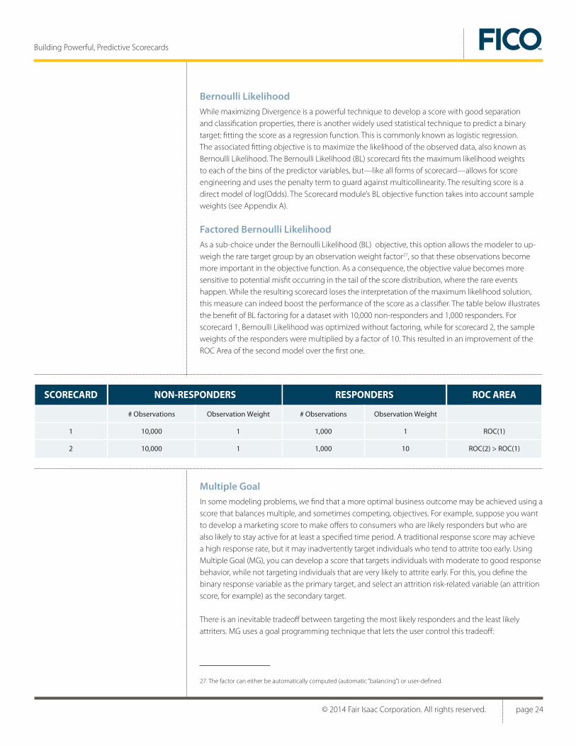
Factored Bernoulli LikelihoodAs a sub-choice under the Bernoulli Likelihood (BL) objective, this option allows the modeler to up-weigh the rare target group by an observation weight factor27, so that these observations become more important in the objective function. As a consequence, the objective value becomes more sensitive to potential misfit occurring in the tail of the score distribution, where the rare events happen. While the resulting scorecard loses the interpretation of the maximum likelihood solution, this measure can indeed boost the performance of the score as a classifier. The table below illustrates the benefit of BL factoring for a dataset with 10,000 non-responders and 1,000 responders. For scorecard 1, Bernoulli Likelihood was optimized without factoring, while for scorecard 2, the sample weights of the responders were multiplied by a factor of 10. This resulted in an improvement of the ROC Area of the second model over the first one.
Multiple GoalIn some modeling problems, we find that a more optimal business outcome may be achieved using a score that balances multiple, and sometimes competing, objectives. For example, suppose you want to develop a marketing score to make offers to consumers who are likely responders but who are also likely to stay active for at least a specified time period. A traditional response score may achieve a high response rate, but it may inadvertently target individuals who tend to attrite too early. Using Multiple Goal (MG), you can develop a score that targets individuals with moderate to good response behavior, while not targeting individuals that are very likely to attrite early. For this, you define the binary response variable as the primary target, and select an attrition risk-related variable (an attrition score, for example) as the secondary target.
There is an inevitable tradeoff between targeting the most likely responders and the least likely attriters. MG uses a goal programming technique that lets the user control this tradeoff:
# Observations Observation Weight Observation Weight
10,000
10,000
1
1
NON-RESPONDERS RESPONDERS
# Observations
1,000
1,000
1
10
ROC AREA
ROC(1)
ROC(2) > ROC(1)
1
2
SCORECARD
27. The factor can either be automatically computed (automatic “balancing”) or user-defined.
© 2014 Fair Isaac Corporation. All rights reserved. page 25
Building Powerful, Predictive Scorecards
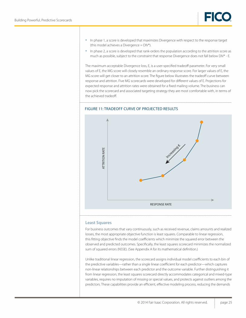
• In phase 1, a score is developed that maximizes Divergence with respect to the response target (this model achieves a Divergence = DIV*).
• In phase 2, a score is developed that rank-orders the population according to the attrition score as much as possible, subject to the constraint that response Divergence does not fall below DIV* - E.
The maximum acceptable Divergence loss, E, is a user-specified tradeoff parameter. For very small values of E, the MG score will closely resemble an ordinary response score. For larger values of E, the MG score will get closer to an attrition score. The figure below illustrates the tradeoff curve between response and attrition. Five MG scorecards were developed for different values of E. Projections for expected response and attrition rates were obtained for a fixed mailing volume. The business can now pick the scorecard and associated targeting strategy they are most comfortable with, in terms of the achieved tradeoff.
Least SquaresFor business outcomes that vary continuously, such as received revenue, claims amounts and realized losses, the most appropriate objective function is least squares. Comparable to linear regression, this fitting objective finds the model coefficients which minimize the squared error between the observed and predicted outcomes. Specifically, the least squares scorecard minimizes the normalized sum of squared errors (NSSE). (See Appendix A for its mathematical definition.)
Unlike traditional linear regression, the scorecard assigns individual model coefficients to each bin of the predictive variables—rather than a single linear coefficient for each predictor—which captures non-linear relationships between each predictor and the outcome variable. Further distinguishing it from linear regression, the least squares scorecard directly accommodates categorical and mixed-type variables, requires no imputation of missing or special values, and protects against outliers among the predictors. These capabilities provide an efficient, effective modeling process, reducing the demands
FIGURE 11: TRADEOFF CURVE OF PROJECTED RESULTS
RESPONSE RATE
ATTR
ITIO
N R
ATE
Incre
asing ε
© 2014 Fair Isaac Corporation. All rights reserved. page 26
Building Powerful, Predictive Scorecards
for up-front data processing and allowing for weaker assumptions on the modeling data. And true to all forms of scorecard, this model also allows for interactive score engineering and provides a penalty term to guard against multicollinearity.
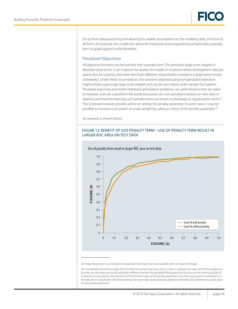
Penalized ObjectivesAll objective functions can be overlaid with a penalty term. This penalizes large score weights in absolute value terms. It can improve the quality of a model in situations where development data are sparse (low bin counts), and when bins from different characteristics overlap to a large extent (multi-collinearity). Under these circumstances, the solutions obtained using non-penalized objectives might exhibit surprisingly large score weights and can be non-robust under sample fluctuations. Penalized objectives pose better behaved optimization problems, can yield solutions that are easier to interpret, and can outperform the predictive power of a non-penalized solution on new data. In statistics and machine learning, such penalty terms are known as shrinkage or regularization terms.28
The Scorecard module provides advice on setting the penalty parameter. In some cases, it may be possible to increase score power on a test sample by judicious choice of the penalty parameter.29
An example is shown below:
FIGURE 12: BENEFIT OF SIZE PENALTY TERM—USE OF PENALTY TERM RESULT IN LARGER ROC AREA ON TEST DATA
Use of penalty term result in larger ROC area on test data
1.0
0.9
0.7
0.5
0.4
0.8
0.6
0.3
0.2
0.1
0
0 0.20.1 0.3 0.4 0.5 0.6 0.7 0.8 0.9 1.0
F(SCORE | G)
F(SC
OR
E | B
)
Score fit with penaltyScore fit without penalty
28. “Ridge Regression” is an example of a regression technique that uses a penalty term to induce shrinkage.
29. A remarkable theoretical insight from the field of machine learning is that, in order to optimize the value of the fitting objective function on new data, one should optimize a different (namely the penalized) fitting objective function on the training sample [3]. In practice, it may require a few iterations to find the best value of the penalty parameter, such that score power is maximized on a test data set. In conjunction with the bootstrap, the user might apply bootstrap-adaptive estimation [5] to determine a good value for the penalty parameter.
© 2014 Fair Isaac Corporation. All rights reserved. page 27
Building Powerful, Predictive Scorecards
Fitting AlgorithmsThe purpose of the fitting algorithm is to solve the constrained optimization problems posed in the prior section. The solution is given by the optimal set of score weights. In the language of mathematical programming, the Scorecard module’s objectives represent quadratic and nonlinear programming (NLP) problems. The Scorecard module provides several parameters and constraint options, with optimization problems each possessing a unique, global optimal solution.30 This is an important consideration, in that general NLP’s are prone to problems related to finding local optima as solutions when they are present; an objective surface with a unique optimum avoids this possibility.
The Scorecard module for FICO® Model Builder uses industrial-grade, efficient quadratic and NLP algorithms for fitting the scorecard, so that the fit is achieved in a reasonable amount of time. The following parameters should be expected to influence the difficulty of the optimization problem and the expected time required for the fit:
• Size of model (number of characteristics and bins)
• Length of development sample (# of records)
• Use of bagging and/or bootstrap validation
• Use of automated variable selection
• Choice of fitting objective function
• Number of engineering constraints
The solutions to the Range Divergence, Bernoulli Likelihood and Multiple Goal objectives require more iterations than the solution to the Divergence and Least Squares objectives.
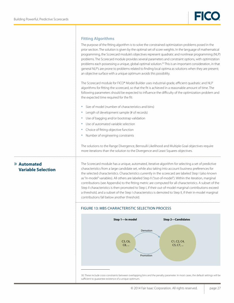
The Scorecard module has a unique, automated, iterative algorithm for selecting a set of predictive characteristics from a large candidate set, while also taking into account business preferences for the selected characteristics. Characteristics currently in the scorecard are labeled Step I (also known as “in-model” variables). All others are labeled Step II (“out-of-model”). Within the iteration, marginal contributions (see Appendix) to the fitting metric are computed for all characteristics. A subset of the Step II characteristics is then promoted to Step I, if their out-of-model marginal contributions exceed a threshold, and a subset of the Step I characteristics is demoted to Step II, if their in-model marginal contributions fall below another threshold.
» Automated Variable Selection
30. These include cross-constraints between overlapping bins and the penalty parameter. In most cases, the default settings will be sufficient to guarantee existence of a unique optimum.
FIGURE 13: MBS CHARACTERISTIC SELECTION PROCESS
C3, C6,C8, ...
C1, C2, C4,C5, C7, ...
Step 1—In model Step 2—Candidates
Demotion
Promotion

© 2014 Fair Isaac Corporation. All rights reserved. page 28
Building Powerful, Predictive Scorecards
The thresholds are user-defined along with an optional assignment of the candidate characteristics to tier groups. The tier groups, along with specific promotion rules for the various tiers, add user control over the selected characteristic mix, as compared to results with a purely data-driven selection. The promotion and demotion process is iterated until there are no more promotions or demotions, or until a maximum number of iterations are reached.
Scoring formulas fit with the Divergence, Range Divergence or Multiple Goal objective functions are on the Weight of Evidence (WOE) scale. Depending on the use of the score, it is often necessary to calibrate the score to directly model probabilities or Log(Odds). A straightforward way to do this is to fit a logistic regression model with the score as the sole predictive variable to predict the binary target.
Let:
The linear model for log(Odds) is:
logOdds = B0 + B1*CB_SCORE (1)
In the above, b0, b1 are intercept and slope parameters which are estimated by the fit. Similarly, a quadratic or higher order model could be attempted, which may in some cases improve on the fit quality.
For this purpose, the Scorecard module offers the Log(Odds) to Score fit task. It provides additional options that allow the analyst to trim the score variable prior to fitting, in order to study fit diagnostic measures and to test hypotheses about the appropriate model (linear or quadratic).
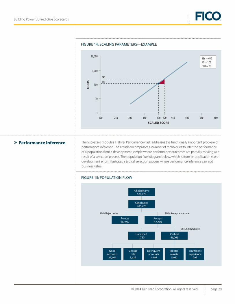
Following the Log(Odds) to Score fit, scores are often transformed to traditional scales, other than log(Odds) or probabilities, using a process called Scaling. The Scorecard module has comprehensive scaling capabilities. Users specify scaling requirements, such as:
• Scaled score value (SSV) associated with required odds value (RO), and
• Required score points to double the odds (PDO), and
• Desired rounding precision of scaled weights, and
• Characteristics whose score weights are desired to be entirely positive.
For example, the user may want a scaled score value of 400 to correspond to odds=120, with 20 score points to double the odds, and using only integer values for score weights. The Scorecard module’s scaling activity will weigh the score and satisfy these user requirements. This will also result in new, scaled weights for the scorecard.
» LogOdds to Score Fitting and Scaling
S : Score variabley = 1{Good} : binary target variable
© 2014 Fair Isaac Corporation. All rights reserved. page 29
Building Powerful, Predictive Scorecards
The Scorecard module’s IP (Infer Performance) task addresses the functionally important problem of performance inference. The IP task encompasses a number of techniques to infer the performance of a population from a development sample where performance outcomes are partially missing as a result of a selection process. The population flow diagram below, which is from an application score development effort, illustrates a typical selection process where performance inference can add business value.
» Performance Inference
FIGURE 14: SCALING PARAMETERS—EXAMPLE
10,000
1,000
100
10
1
200 300 350250 400 450 500 550420 600
SCALED SCORE
OD
DS 120
240
SSV = 400RO = 120PDO = 20
FIGURE 15: POPULATION FLOW
All applicants528,078
Candidates485,723
Rejects437,927
Accepts47,796
Cashed46,066
Uncashed1,730
Goodaccounts
37,664
Indeter-minate5,032
Insufficientexperience
295
96% Cashed rate
10% Acceptance rate90% Reject rate
Delinquentaccounts
1,446
Chargeoffs
1,629

© 2014 Fair Isaac Corporation. All rights reserved. page 30
Building Powerful, Predictive Scorecards
“Candidates” refers to the population for which a representative development sample has been obtained. This is the population to which the scoring system will be applied, barring some policy exclusions from scoring. We’re not interested in the issue of policy exclusions here, and we will call the candidates the “Through-The-Door” (TTD) population. The key issue is that performance outcomes are available only for a fraction (here, 9.6%) of the TTD population, due to the fact that a large number of applicants were rejected under the previous policy, and also a small fraction stayed uncashed.
The ProblemWe have a development sample representing the TTD population, where part of the sample has known Good/Bad performance (those who where accepted and cashed are summarized as “knowns”), and part of the sample has unknown binary performance (those who were rejected or stayed uncashed are summarized as “unknowns”). The objective for score development is to obtain credible performance estimates for the entire TTD population
Often, the problem arises that the knowns alone may not constitute a representative sample.31 Then it can be dangerous to drop the unknowns out of the score development, causing the developed score model to be biased and inappropriate for estimating the likelihood of loan default of all future TTD applicants. To develop a credible scoring system, the score should be developed based on a representative sample of the TTD population. This requires inferring the performance of the unknowns and using the inferred observations as part of the final score development. Reliable inference methods can be quite complex, depending on the nature of the selection process, the available data, and the score development technique. Two examples of applications of performance inference may serve to illustrate some of the various options.
Performance Inference Using External InformationThe main idea here is to use a credit bureau (CB) score, obtained at a suitable point in time, to infer how the rejects would have performed had they been accepted. The key assumption is that the CB score contains information about their likely performance, had they been granted the loan.
To make this idea work, we need to calibrate the CB score to the TTD population for the score development. For this we use a representative sample of the knowns to fit a Log(Odds) model to the CB score. A simple model might be:
logOdds = B0 + B1*CB_SCORE (1)
Since the FICO® Score is a valuable source of information, there will be a significant positive coefficient B1. For a given unknown observation, for which we have the CB score, we use the model to compute the probability pG that this unknown observation would have been a Good:
pG = 1 / (1 + exp{-(B0 + B1*CB_SCORE)} ) (2)
Note that the B0, B1, and pG do not constitute the end product of reject inference. Our ultimate goal is a scoring model that works for the TTD population. The above parameters constitute, however, a key step on the way to a successful final score development. These estimates are then used by the Scorecard module in an iterative process to infer the performance of the TTD population.
31. An alternative to Performance Inference is to randomly accept a sample of the population that would otherwise be rejected and to include this sample in score development. But of course, this cannot be done in the modeling laboratory after the fact, it must have been part of the years-ago business process that generated today’s modeling data.

© 2014 Fair Isaac Corporation. All rights reserved. page 31
Building Powerful, Predictive Scorecards
Performance Inference Using Domain ExpertiseHere the assumption is that no supplementary data are available. The key idea is to carefully craft a score model (called KN_SCORE) on the known population such that it can be used for assigning credible performances to the unknowns. Analogous to the above, we have now:
logOdds = C0 + C1*KN_SCORE (3)
pG’ = 1 / (1 + exp{-(C0 + C1*KN_SCORE)} ) (4)
Again, C0, C1, and pG’ represent intermediate results. These parameters will be used by Scorecard module in an iterative parceling process to infer the performance of the TTD population. KN_SCORE is called the “parcel score” as it drives the initial assignment (or parceling) of credible performance to the unknowns.
Key to successful reject inference in this example is the development of a credible KN_SCORE. This often requires the analyst to abstain from developing the most predictive score model for the knowns, but to rely to a greater extent on domain knowledge and suitable score engineering. For example, the previous selection process may have “cherry picked” among students (accepting not all students, but only a special subset known to be better payers than their peers, using criteria that are not actually visible in our model development data). As a consequence, the score developed on the known population might assign unreasonably good performances to the students among the TTD population (they might be inferred to be less risky than some trustworthy professional occupations). The analyst might also gain additional evidence for “cherry picking,” based on a very low observed odds of accepting students versus rejecting them, and possibly this insight can be validated through existing domain knowledge. If there is strong evidence that only the “crème” of the student population is known, an experienced analyst will counteract possible selection bias by engineering the score for the knowns in suitable ways, such that the students are assigned more appropriate performances. A simple engineering option is not to include the occupation in the development of the KN_SCORE. More sophisticated model engineering options exist, which allow reducing possible bias more selectively. Any engineering may cause KN_SCORE to be less predictive on the known development data set than it could be when fitting an un-engineered model. But it is reasonable to trade off a limited loss in predictive power against a reduction of bias. After all, KN_SCORE is used only to infer the unknowns, and the final TTD score model might be developed including a different set of predictors.
In summary, judicious choice of predictive characteristics and score engineering are instrumental for counteracting possible selection bias when developing KN_SCORE. For this very reason, it is often preferable to develop KN_SCORE using the Scorecard module rather than other predictive technologies, because the Scorecard module provides flexible score engineering capabilities to handle possible bias in data.
Note that the Scorecard module allows for multiple simultaneous views of the development data (such as Good versus Bad Odds, and Accept versus Reject Odds), which provides good insights into the previous selection process, and can be of help in spotting possible selection bias.
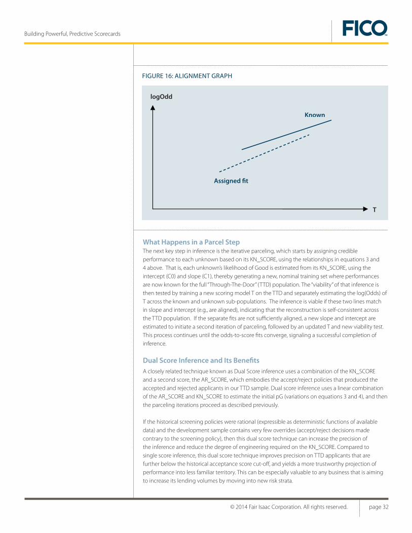
© 2014 Fair Isaac Corporation. All rights reserved. page 32
Building Powerful, Predictive Scorecards
What Happens in a Parcel StepThe next key step in inference is the iterative parceling, which starts by assigning credible performance to each unknown based on its KN_SCORE, using the relationships in equations 3 and 4 above. That is, each unknown’s likelihood of Good is estimated from its KN_SCORE, using the intercept (C0) and slope (C1), thereby generating a new, nominal training set where performances are now known for the full “Through-The-Door” (TTD) population. The “viability” of that inference is then tested by training a new scoring model T on the TTD and separately estimating the log(Odds) of T across the known and unknown sub-populations. The inference is viable if these two lines match in slope and intercept (e.g., are aligned), indicating that the reconstruction is self-consistent across the TTD population. If the separate fits are not sufficiently aligned, a new slope and intercept are estimated to initiate a second iteration of parceling, followed by an updated T and new viability test. This process continues until the odds-to-score fits converge, signaling a successful completion of inference.
Dual Score Inference and Its BenefitsA closely related technique known as Dual Score inference uses a combination of the KN_SCORE and a second score, the AR_SCORE, which embodies the accept/reject policies that produced the accepted and rejected applicants in our TTD sample. Dual score inference uses a linear combination of the AR_SCORE and KN_SCORE to estimate the initial pG (variations on equations 3 and 4), and then the parceling iterations proceed as described previously.
If the historical screening policies were rational (expressible as deterministic functions of available data) and the development sample contains very few overrides (accept/reject decisions made contrary to the screening policy), then this dual score technique can increase the precision of the inference and reduce the degree of engineering required on the KN_SCORE. Compared to single score inference, this dual score technique improves precision on TTD applicants that are further below the historical acceptance score cut-off, and yields a more trustworthy projection of performance into less familiar territory. This can be especially valuable to any business that is aiming to increase its lending volumes by moving into new risk strata.
FIGURE 16: ALIGNMENT GRAPH
Assigned �t
Known
logOdd
T
© 2014 Fair Isaac Corporation. All rights reserved. page 33
Building Powerful, Predictive Scorecards
Summary of Performance InferencePerformance inference can add business value to a score or model development process by reducing the impact of selection bias on the final model. This process is not a “push button” algorithm, but is affected by the nature of the previous selection criteria, data availability, and domain knowledge. Performance inference is impossible without making certain assumptions. The details of reject inference in the Scorecard module are based on the concept of score viability.
Performance inference may be useful for a wider range of applications than developing Good/Bad models for estimating default risk in credit originations. For example, in marketing applications, only those accounts that previously received an offer carry information on their responses or non-responses, but we would like to develop a response model that works for the entire population. For those that didn’t receive an offer, we may still have financial and demographic information that can help with inferring their likely responses had they received an offer.
Developing a powerful scorecard is a balancing act. First, the model must reflect the development data well enough to capture the relevant effects (nonlinearities, interactions) inherent in the underlying relationship between predictors and target variable. Second, the model must not follow the development data so closely as to pick up spurious effects or noise that could misrepresent the underlying relationship. In applied statistics, this is sometimes referred to as the “Bias-Variance tradeoff.” It is perhaps not surprising that with modern, flexible modeling technologies, such as the family of scorecards, the first issue of “under-fitting” causes few worries. The emphasis of model validation is placed squarely on the second issue: to avoid the pitfalls of “over-fitting” the data. This is especially important if the development sample for building the scorecard is small.
Every trained model has to be validated prior to deployment to obtain confidence in the satisfactory future performance of the model. Validation prior to deployment can only be based on a snapshot of historic data, and thus relies on the assumption that this snapshot in time provides a good representation of the future population32. We will describe two approaches to obtaining unbiased estimates of future model performance below.
The ProblemIn the following we will use the symbol M to denote the model performance measure of interest. For example, M could be Divergence, or area under the ROC curve, both of which we want to be large for the population on which the model will be applied. We call this quantity M
pop. The problem is that
we don’t know Mpop
. But we can try to estimate it by observing the value of M on some sample. An obvious (but somewhat misguided) option is to observe M on the training sample, which is used to develop the score. We call this quantity M
trn The fundamental problem is that M
trn is an over-
optimistically biased estimate of Mpop
:
Mpop
= Mdev
– bias ; where bias > 0
This is due to the fact that the developed model exhibits some amount of over-fitting to the noise in the development data set, which will not be replicated in other data sets. So, how can we obtain unbiased estimates of M
pop?
» Bootstrap Validation and Bagging
32. The model developer is responsible for drawing a development sample that is representative of the likely future population. Population composition and model performance can be monitored or tracked over time in order to detect possible deviations. This is not discussed here.
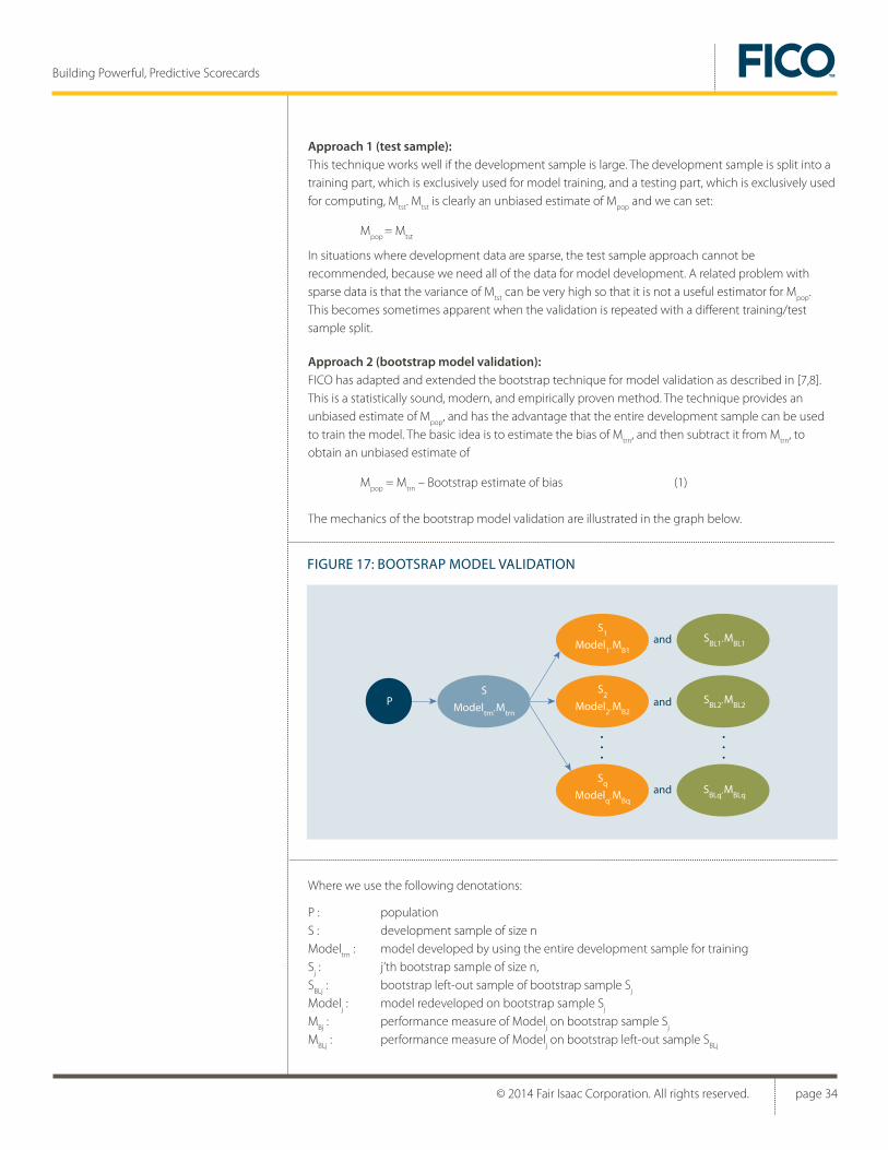
© 2014 Fair Isaac Corporation. All rights reserved. page 34
Building Powerful, Predictive Scorecards
Approach 1 (test sample):This technique works well if the development sample is large. The development sample is split into a training part, which is exclusively used for model training, and a testing part, which is exclusively used for computing, M
tst. M
tst is clearly an unbiased estimate of M
pop and we can set:
Mpop
= Mtst
In situations where development data are sparse, the test sample approach cannot be recommended, because we need all of the data for model development. A related problem with sparse data is that the variance of M
tst can be very high so that it is not a useful estimator for M
pop.
This becomes sometimes apparent when the validation is repeated with a different training/test sample split.
Approach 2 (bootstrap model validation):FICO has adapted and extended the bootstrap technique for model validation as described in [7,8]. This is a statistically sound, modern, and empirically proven method. The technique provides an unbiased estimate of M
pop, and has the advantage that the entire development sample can be used
to train the model. The basic idea is to estimate the bias of Mtrn
, and then subtract it from Mtrn
, to obtain an unbiased estimate of
Mpop
= Mtrn
– Bootstrap estimate of bias (1)
The mechanics of the bootstrap model validation are illustrated in the graph below.
Where we use the following denotations:
P : populationS : development sample of size nModel
trn : model developed by using the entire development sample for training
Sj : j’th bootstrap sample of size n,
SBLj
: bootstrap left-out sample of bootstrap sample Sj
Modelj : model redeveloped on bootstrap sample S
j
MBj : performance measure of Model
j on bootstrap sample S
j
MBLj
: performance measure of Modelj on bootstrap left-out sample S
BLj
FIGURE 17: BOOTSRAP MODEL VALIDATION
S2
Model2’
MB2
P
S1
Model1’
MB1
Sq
Modelq’
MBq
SBL1’
MBL1
SBL2’
MBL2
SBLq’
MBLq
S
Modeltrn’
Mtrn
•••
•••
and
and
and

© 2014 Fair Isaac Corporation. All rights reserved. page 35
The bootstrap estimate of bias is derived using a series of randomly drawn samples from the full development dataset. In the first iteration, n observations are selected from the development data, with replacement. In this process, some observations will be drawn multiple times, while other observations will not be selected at all. Every selected observation (including duplicates) is written to a bootstrap sample. Observations that were not selected at all are written to a bootstrap left-out sample.
Next, new model weights are trained from the bootstrap sample, and its in-sample performance is evaluated using the same data. In addition, the new model’s out-of-sample performance is evaluated using the left-out sample set. The difference between in-sample performance (which tends to be higher) and out-of-sample performance (which tends to be lower) is calculated. This process of resampling, training and evaluating is repeated q times.
The central idea behind the bootstrap bias estimator is to substitute the observed performance difference (MBj - MBLj) for the bias, barring a correction factor. The “632 Bootstrap Bias Estimator” [7] is:
Inserting this result in (1) yields the desired unbiased estimate of Mpop
:
In order to obtain a good bootstrap estimate bias, q has to be sufficiently large, thereby sampling, and averaging over, many observed performance differences. This method provides not only a reliable estimate of bias, and therefore of M
pop, but also a confidence interval around M
pop. The Scorecard
module uses a statistical criterion to decide the appropriate number of repetitions q, stopping when the variability of the error estimate falls beneath a threshold. The user may control that threshold, as well as minimum and maximum number of iterations to attempt.
Building Powerful, Predictive Scorecards
∑
∑ ∑
=
= =
∗−∗≅
∗−∗=
q
1jBLjq
1trn
q
1j
q
1jBLjq
1Bjq
1
M.632M.632
M.632M.632
Bootstrap estimate of bias
∑=
∗+∗=
−=q
1jBLjq
1trn
trnpop
M.632M.368
MM Bootstrap estimate of bias
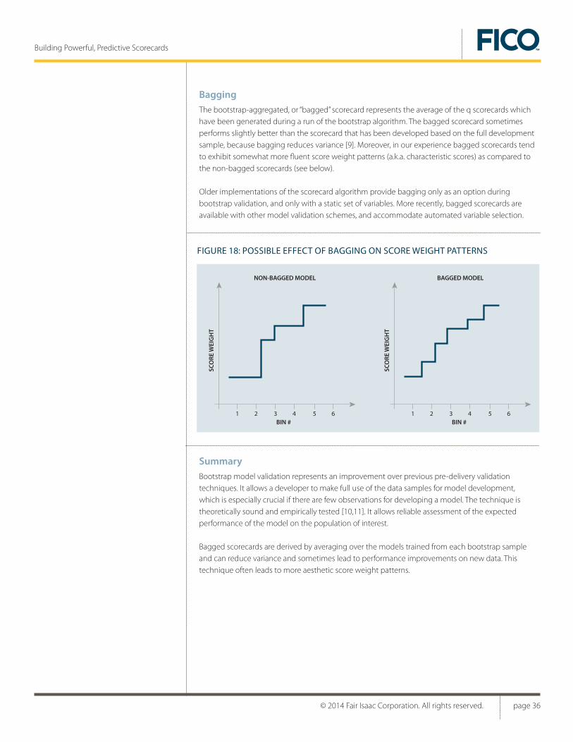
© 2014 Fair Isaac Corporation. All rights reserved. page 36
Building Powerful, Predictive Scorecards
BaggingThe bootstrap-aggregated, or “bagged” scorecard represents the average of the q scorecards which have been generated during a run of the bootstrap algorithm. The bagged scorecard sometimes performs slightly better than the scorecard that has been developed based on the full development sample, because bagging reduces variance [9]. Moreover, in our experience bagged scorecards tend to exhibit somewhat more fluent score weight patterns (a.k.a. characteristic scores) as compared to the non-bagged scorecards (see below).
Older implementations of the scorecard algorithm provide bagging only as an option during bootstrap validation, and only with a static set of variables. More recently, bagged scorecards are available with other model validation schemes, and accommodate automated variable selection.
SummaryBootstrap model validation represents an improvement over previous pre-delivery validation techniques. It allows a developer to make full use of the data samples for model development, which is especially crucial if there are few observations for developing a model. The technique is theoretically sound and empirically tested [10,11]. It allows reliable assessment of the expected performance of the model on the population of interest.
Bagged scorecards are derived by averaging over the models trained from each bootstrap sample and can reduce variance and sometimes lead to performance improvements on new data. This technique often leads to more aesthetic score weight patterns.
FIGURE 18: POSSIBLE EFFECT OF BAGGING ON SCORE WEIGHT PATTERNS
1 2 3 4 5 6
SCO
RE W
EIG
HT
BIN #
BAGGED MODEL
1 2 3 4 5 6
SCO
RE W
EIG
HT
BIN #
NON-BAGGED MODEL

© 2014 Fair Isaac Corporation. All rights reserved. page 37
Principal SetsAlso known as outcome classes, the principal sets represent the Scorecard module’s mechanism for dichotomizing a business outcome into a binary classing scheme33, denoted as:
• Left Principal Set L
• Right Principal Set R1
In some score development projects, the observed business outcome can be clearly identified as binary, such as “Good” vs. “Bad”, or “Responder” vs. ”No Response.” In this case there is no ambiguity for defining the principal sets. If the business outcomes take on more values, the score developer organizes them into the principal sets. For example, the target variable available from a database for credit application risk score development may assume the values γ ε {2,3,4,7,8} which denote, respectively, individuals that were declined credit, experienced bankruptcy, were ever 60+ days delinquent, were never 60+ days delinquent, or were offered credit but remained uncashed. The scorecard developer may define L = {7} (never seriously delinquent = “Good”) and R = {3,4} (bankrupt or ever seriously delinquent = “Bad”).
The Scorecard module allows analysts to define multiple principal sets. This allows for multiple views of the data. For example, individuals could also be dichotomized into “Accepts” and “Rejects,” giving rise to additional principal sets L’ = {3,4,7,8} (accepted individuals) and R’ = {2} (individuals that were rejected). In an application scorecard development it can be important to gain insights into the selection process that generated the development sample. For this, it is relevant to know the Accept/Reject Odds for the characteristic bins. Definition of multiple performance sets plays a particularly important role in performance inference.
Characteristic-Level Statistics for Binary Outcome ProblemsThis section defines several key statistical quantities which are defined on the bin and characteristic level. Consider a characteristic with bins i = 1,2,...,q.
Factored Counts are defined by:34
Building Powerful, Predictive Scorecards
appendix A
» Defining Statistical Quantities Used by Scorecard for FICO® Model Builder
nL
= Number of Goods in the population
nR
= Number of Bads in the population
nLi
= Number of Goods in bin i
nRi = Number of Bads in bin i
n = nL+n
R = Number of individuals in the population
33. As a convention, L typically stands for observations that are classified as “Good” or desirable (e.g. good credit standing, responds to a mail campaign, a retained account, etc.), and R stands for observations that are classified as “Bad” or undesirable (a delinquent account, a non-responder, an attrition, etc.). More generally, L is the “High scoring set” (the outcome we associate with the high end of the scoring range), and R is the “Low scoring set” (outcome associated with the low end of the scoring range).
34. The Scorecard module takes into account the sample weight generated from a possible stratified sampling process during which model development observations were generated from a larger population. A value of the sample weight is associated with each observation. Scorecard then generates counts which are appropriately factored up to the population.

© 2014 Fair Isaac Corporation. All rights reserved. page 38
Building Powerful, Predictive Scorecards
Empirical frequency distribution versions of these counts are:
Weight of evidence35 of bin is defined as:
Where log denotes the natural logarithm. The bins should contain a reasonable number of good and bad individuals to make this a reliable statistic. A value of WOE = 0 means that the odds for this bin are no different from the odds of the population average, while positive or negative values mean that this bin represents a better or worse risk than the population average.
Information Value36 (IV) of a binned variable is defined as:
IV Contribution of bin i is defined as:
The IV of a binned variable indicates its stand-alone predictive power for telling apart L from R.
Characteristic-Level Statistics for Continuous Outcome Problems
When the target variable is continuous, we have a continuum of response values, rather than two discrete outcome classes. For such problems, the metrics are adapted from the prior definitions.
Factored Counts are simply defined by
n = Number of individuals in the population n
i = Number of individuals in bin i
Empirical frequency distribution versions of these counts are:
f(i) = Percentage of individuals falling into bin i ý = Mean value of response value y for all individuals ý(i) = Mean value of response value y for individuals in bin i
( )
( )n
nif
n
nif
B
BiG
G
GiL
100
100
= Percentage of individuals in G that fall into bin i=
= Percentage of individuals in L that fall into bin i=
=)(
)(log)(
if
if iWOE
G
L[ ]
[ ](i) (i)−= ∑
= )(
)(log
1001 if
ifffIV
G
Lq
i
RL
[ ](i) (i)−=
)(
)(log
100 if
ifffIVcontrib
G
LRL
35. The notion of WOE arises from applying Bayes Theorem, which allows us to re-express the logarithm of the odds of a bin as follows: ( Logarithm of odds of bin i ) = ( Logarithm of Population Odds ) + ( WOE of bin i )WOE thus represents the additional knowledge gained about the odds of an individual over and above the population odds, after we learn that this individual falls into a specific bin.
36. The concept of Information Value has its roots in Information Theory [4]. It measures the distance between two distributions (here, between the discrete distributions of Goods and Bads over a set of bins).

© 2014 Fair Isaac Corporation. All rights reserved. page 39
Building Powerful, Predictive Scorecards
For continuous outcome problems, Weight of Evidence of a bin is defined as:
WOE(i) = ý(i) – ý
Like its analog in the binary outcome problem, this statistic is a reasonable estimate when the bin contains a sufficient number of individuals, and its sign indicates the current bin’s relationship to the population average. A WOE of 0 indicates that the bin carriers precisely the same mean response as the total population, while positive (negative) WOEs indicate bins with higher (lower) mean response than the general population.
The formulae for Information Value and IV Contribution are natural adaptations of those of binary outcomes, using the WOE statistic suitable to the continuous response variable.
IV Contribution of bin i is defined as:
IVcontrib
= f(i) [ ý(i) – ý ] / 100
As with the binary outcome definition, the Information Value for the continuous target is simply the sum of IV
contrib over all the bins of the variable. The IV of a variable indicates its stand-alone ability
to separate low and high values of the response variable, y.
Objective functions
Divergence of a score is defined as:
The objective is to maximize Divergence, which achieves a good separation.
Bernoulli Likelihood of a score is defined as:
Div(Score) = (µL − µR)
2
(σ G + σ B )/22 2
µL
= E[Score | L], the mean of the score conditioned on Lµ
R = E[Score | R], the mean of the score conditioned on R
σ = V[Score | L], the mean of the score conditioned on Lσ = V[Score | R], the mean of the score conditioned on R
2
2
R
L
BL(Score) = [p(xi)] [1 − p(xi)]∏w
i y
inw
i (1− y
i)
i=1

© 2014 Fair Isaac Corporation. All rights reserved. page 40
Building Powerful, Predictive Scorecards
Where:
The objective is to maximize the Bernoulli Likelihood, which achieves a good approximation of the observed frequencies by the predicted probabilities. The numerical values of Bernoulli Likelihood are not easy to interpret. For this reason, we provide the Normalized Log(Likelihood) (NLL) measure. This measures the performance of a score relative to the performance of an “intercept-only” model:
Smaller values of NLL indicate a better fit. Its typical value range is between 0 and 1.
The weight given to each observation in the objective function is typically the sample weight. However, for Factored Bernoulli Likelihood, the sample weights of all observations falling into one principal set are up-weighted by some common factor, so that the weighting scheme used in the objective function now depends on new observation weights.
Normalized Sum of Squared Errors of a score is defined as:
where: • n is the number of data points
• wi is the sample weight.
• yi is the actual response of the data
• (y-hat of i) is the model predicted response.
• is the sample mean, e.g.,
This measure generally ranges between 0 and 1, with 0 representing zero error, and perfect estimation. Hence, the least squares objective function seeks to minimize this metric.
Marginal ContributionWhile Information Value measures a variable’s stand-alone ability to predict the target, Marginal Contribution (MC) estimates a variable’s unique contribution to the total predictive power of a model. In the Scorecard module, marginal contribution is calculated for both in-model and out-of-model variables, by estimating the impact of removing or adding that variable while holding the rest of the model constant. The calculation of MC depends on the choice of fitting objective function.
The In-Model Marginal Contribution of a scorecard characteristic is defined as:
• For divergence-related objective functions (Divergence, Multiple Goal, and Range Divergence), the MC is the reduction of divergence that would be incurred by removing this variable from the scorecard, while leaving all other score weights at their current values.
p(xi ) : Probability that observation i ∈ L
wi : weight of observation i
yi : indicator indicator for observation i ∈ L
NLL =log(BL)
log(BLintercept−only)
wi ( y
i - y
i )2 / w
i ( y
i - y )2 ^∑
=
n
1i∑=
n
1n
_
y _
yi
^
y = yi ∑
=
n
1i
_ 1n_

© 2014 Fair Isaac Corporation. All rights reserved. page 41
Building Powerful, Predictive Scorecards
• For the Least Squares objective function, the MC is the increase of the Normalized Sum of Squared Error (NSSE) that would be incurred by removing this variable from the scorecard, while leaving all other score weights at their current values.
• For the Bernoulli Likelihood objective function, the MC is the increase of the Normalized Log Likelihood (NLL) that would be incurred by removing this variable from the scorecard, while leaving all other score weights at their current values.
By way of example, for divergence models, the in-model marginal contribution, MCI(j), of each in-model variable j is estimated as follows:
S = Vector of bin-level coefficients optimizing the objective function S(j) = Vector of bin-level coefficients drawn from S, but with zeros for the bins of characteristic j Div(S) = Divergence of model resulting from coefficients S Div(S(j)) = Divergence of model resulting from coefficients S(j) MCI(j) = Div(S) – Div(S(j))
Given these definitions, it should be clear that the MC is on the same scale as the objective function itself. It is also worth noting that in-model MC is not a direct measure of the change in objective function that would result from formally dropping the variable and re-optimizing all remaining bin-level coefficients. Rather, it indicates the relative strength of each variable within the current model.
In the Scorecard module’s automated variable selection algorithm, the in-model MC is used to determine which, if any, variables fail the stay-in threshold and will be dropped in the next iteration of model training.
The Out-of-Model Marginal Contribution of a scorecard characteristic is a proxy for the expected increase in Divergence (reduction of NSSE, or reduction in NLL) by including this characteristic into the scorecard.
As with in-model, we start with
S = Vector of bin-level coefficients optimizing the objective function
And then, for each out-of-model variable k, MCO(k) is estimated as:
S(k) = Expanded vector of bin-level weights, adding new optimal coefficients for the bins of variable k, while leaving the original coefficients from S unchanged
MCO(k) = Div(S(k)) – Div(S)
As such, out-of-model MC is not a direct measure of the change in objective function that would come from formally adding variable k to the model and completely re-optimizing all bin-level coefficients. Nonetheless, it does provide a useful relative ranking of the potential signal strength remaining in the out-of-model variables.
In the Scorecard module’s automated variable selection algorithm, the out-of-model MC is used to rank and select variables for inclusion in the next iteration of model training.
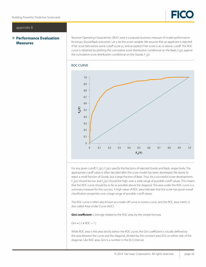
© 2014 Fair Isaac Corporation. All rights reserved. page 42
Building Powerful, Predictive Scorecards
appendix B
Receiver Operating Characteristic (ROC) area is a popular business measure of model performance for binary (Good/Bad) outcomes. Let y be the score variable. We assume that an applicant is rejected if her score falls below some cutoff score yc, and accepted if her score is at, or above, cutoff. The ROC curve is obtained by plotting the cumulative score distribution conditional on the Bads, F
B(y), against
the cumulative score distribution conditional on the Goods, FG(y):
For any given cutoff, FG(yc), F
B(yc) specify the fractions of rejected Goods and Bads, respectively. The
appropriate cutoff value is often decided after the score model has been developed. We desire to reject a small fraction of Goods, but a large fraction of Bads. Thus, for a successful score development, F
G(yc) should be low and F
B(yc) should be high, over a wide range of possible cutoff values. This means
that the ROC curve should be as far as possible above the diagonal. The area under the ROC curve is a summary measure for this success. A high value of ROC area indicates that the score has good overall classification properties over a large range of possible cutoff values.
The ROC curve is often also known as a trade-off curve or Lorenz curve, and the ROC area metric is also called Area Under Curve (AUC).
Gini coefficient is strongly related to the ROC area, by the simple formula
Gini = | 2 × ROC − 1 |
While ROC area is the area strictly below the ROC curve, the Gini coefficient is visually defined by the area between the curve and the diagonal, divided by the constant area (0.5) on either side of the diagonal. Like ROC area, Gini is a number in the [0,1] interval.
» Performance Evaluation Measures
ROC CURVE
1.0
0.9
0.7
0.5
0.4
0.8
0.6
0.3
0.2
0.1
0
0 0.20.1 0.3 0.4 0.5 0.6 0.7 0.8 0.9 1.0
FG(Y)
F B(Y)

© 2014 Fair Isaac Corporation. All rights reserved. page 43
Building Powerful, Predictive Scorecards
Due to a peculiarity in ROC area, Gini is often regarded as a better measure for comparing the relative strength of two or more models against the same population and binary target. A model with a Gini coefficient of 1 is a perfect classifier, and a model with Gini of 0 is a completely useless classifier. Thus, higher Gini always indicates the stronger model.
However, this is not always the case with ROC area. In our example above, if we imagine reversing the orientation of our scoring model (e.g., by simply multiplying by -1), this model would award high scores for future Bads and low scores for future Goods. In terms of ROC curve, this simply flips the x- and y- axes, giving us a curve below the diagonal and hence with much less total area beneath it. Nonetheless, this model possesses rank-ordering qualities identical to those of the original score, and is thus an equally strong classifier.
So, while ROC area also falls in the [0,1] interval, its peculiar property is that both 0 and 1 represent perfect classifiers, and the midpoint (0.5) represents a completely useless classifier. Unless you know that any compared models are identically oriented to your binary target, you must exercise care when comparing two models by their ROC area.

© 2014 Fair Isaac Corporation. All rights reserved. page 44
Building Powerful, Predictive Scorecards
appendix C
Multicollinearity refers to the relationships which may exist among the independent variables (predictors) of a predictive modeling problem. Most commonly, the presence of multicollinearity among the predictors may yield non-intuitive model coefficients or puzzlingly low significance for predictors known to strongly correlate with the target, and generally indicate instability in the model.
Multicollinearity can be regarded as a property of the data itself, and different modeling techniques may be more or less sensitive to its effects. Practitioners of traditional logistic regression often examine their models for evidence of multicollinearity, such as sign reversals in the model’s coefficients and high variance inflation factors among the model’s predictors, which suggest instability in the model’s solution. The mathematical formulation, optimization and diagnostics of a scorecard provide the analyst with a number of unique tools to identify, avoid and mollify the influence of multicollinearity when building a scorecard.
The Model Builder scorecard formulation is a generalized additive model which discretizes each nominal predictor into a collection of bins. Hence, each scorecard predictor becomes a mutually exclusive and collectively exhaustive partition of the population. A common practice in binned logistic regression with such partitions is to use “N-1” binary indicators, by arbitrarily dropping one bin to eliminate an undesirable degree of freedom (and otherwise guaranteed source of multicollinearity). In the scorecard optimization, this unwanted degree of freedom is instead eliminated by automatically applying a centering constraint, which fixes the weights within the zero-centered weight-of-evidence scale and retains a complete picture of the predictor’s N bins. This property of the scorecard formulation eliminates what would certainly become an ill-conditioned problem.
Perfect and near-perfect collinearities among in-model predictors are also automatically detected by the Model Builder scorecard algorithm, to guard against unstable solutions. At each step of the optimization, any bins which exhibit perfect collinearity across the model’s predictors are automatically cross-constrained to equally divide the total weight. Pairs of bins with strong but less-than-perfect overlap can be automatically detected (by lowering the overlap threshold below 100%), and may be manually cross-restricted by the user. Whether set by the algorithm or the user, these cross-constraints prevent any pair of bins from producing needlessly divergent weights and ensure the existence and stability of a solution.
Furthermore, the scorecard weights-optimization algorithm provides a user-adjustable penalty parameter, to penalize large weight values, and thus provide a further guard against divergent model coefficients, which is a hallmark of multicollinearity. This penalized optimization is a form of regularization which turns an otherwise ill-defined optimization problem into a well-defined problem with a unique solution. Taken together, the features of the scorecard’s mathematical program and its optimization yield robust solutions even in the presence of collinear predictors.
Finally, a scorecard’s diagnostic reports will highlight the presence and influence of collinear predictors, and the analyst may take a number of model engineering steps to mollify their influence on the scorecard. For example, any cross-variable bins with perfect or near-perfect collinearity are detected and reported in the Cross-Variable Constraints table, as are any manual cross-constraints added by the analyst.
» Scorecards and Multicolinearity

© 2014 Fair Isaac Corporation. All rights reserved. page 45
Building Powerful, Predictive Scorecards
The model training report will reveal the influence of any remaining multicollinearity among the in-model predictors to the scorecard modeler and reviewer. This report clearly presents with the solution weight (a multivariate optimization), immediately adjacent to the stand-alone weight-of-evidence (WOE). Any reversals of sign or large discrepancies in magnitude between weight and WOE provide the analyst clear evidence of remaining collinearity in each model train. Such reversals may be immediately remedied by the analyst with scorecard engineering techniques: the variable containing the bin may be simply dropped from the model, the bin in question may be pattern constrained to receive the appropriate sign or limit its magnitude, the bin may be individually neutralized by enforcing a zeroing (“no information”) constraint, the bin may be cross-restricted to a sibling bin of another in-model variable, or the penalty term for the whole scorecard may be increased. Armed with these simple engineering techniques, the analyst may achieve a powerfully predictive scorecard, ensure the existence and stability of solutions, and clearly document all aspects of the model’s engineering, even in the face of collinear predictors.
To conclude, although the development data may often contain collinearities among the candidate predictive variables, the scorecard model provides a unique combination of automatic tests, regularization, clear diagnostic reporting, and transparent engineering actions to produce robust, highly predictive scorecards models.

Building Powerful, Predictive Scorecards
[1] “Generalized Additive Models.” T.J. Hastie, R.J. Tibshirani, 1990. Chapman & Hall/CRC.
[2] FICO. Using Segmented Models for Better Decisions, March 2014.
[3] “The Nature of Statistical Learning Theory.” V.N. Vapnik, 1995. Springer.
[4] “Information Theory and Statistics.” S. Kullback, 1959. John Wiley.
[5] “An Introduction to the Bootstrap.” B. Efron, R.J. Tibshirani, 1998. CRC Press LLC.
[6] FICO. A Discussion of Data Analysis, Prediction, and Decision Techniques, August 2012.
[7] Efron, B. (1983). Estimating the Error Rate of a Prediction Rule: Improvement on Cross-Validation. J. Amer. Statist, Assoc., 78, 316-331.
[8] Efron, B. and Tibshirani, R. (1997). Improvements on Cross-Validation: The .632+ Bootstrap. Method. J. Amer. Statist, Assoc., 92, 548-560.
[9] Breiman, L. Bagging predictors. Machine Learning, 24:123, 1996.
[10] Efron, B. and Tibshirani, R. (1993). An Introduction to the Bootstrap. Chapman & Hall.
[11] Efron, B. & Tibshirani, R. J., A Leisurly Look at the Bootstrap, the Jackknife, and Cross-Validation. The Americal Statistician, February 1983, Vol.37, No.1.
references
For more information North America Latin America & Caribbean Europe, Middle East & Africa Asia Pacificwww.fico.com +1 888 342 6336 +55 11 5189 8222 +44 (0) 207 940 8718 +65 6422 7700 [email protected] [email protected] [email protected] [email protected]
FICO and “Make every decision count” are trademarks or registered trademarks of Fair Isaac Corporation in the United States and in other countries. Other product and company names herein may be trademarks of their respective owners. © 2014 Fair Isaac Corporation. All rights reserved.
1991WP 04/14 PDF
FICO (NYSE: FICO) is a leading analytics software company, helping businesses in 90+ countries make better decisions that drive higher levels of growth, profitability and customer satisfaction. The company’s groundbreaking use of Big Data and mathematical algorithms to predict consumer behavior has transformed entire industries. FICO provides analytics software and tools used across multiple industries to manage risk, fight fraud, build more profitable customer relationships, optimize operations and meet strict government regulations. Many of our products reach industry-wide adoption—such as the FICO® Score, the standard measure of consumer credit risk in the United States. FICO solutions leverage open-source standards and cloud computing to maximize flexibility, speed deployment and reduce costs. The company also helps millions of people manage their personal credit health. Learn more at www.fico.com.