AD-A267 090

Technical Report 1575September 1992

Broadband ConventionalBeamformingIncorporating AdaptiveEqualization

Richard C. North

I -S B •UL 2 1993~

Approved for publdo release; dtrlbutlon Is urMlted.

93--16587

Technical Report 1575September 1992

Broadband Conventional BeamformingIncorporating Adaptive Equalization

Richard C. North

NAVAL COMMAND, CONTROL ANDOCEAN SURVEILLANCE CENTER

RDT&E DIVISIONSan Diego, California 92152-5001

J. D. FONTANA, CAPT, USN R.T. SHEARERCommanding Officer Executive Director

ADMINISTRATIVE INFORMATION

This work, conducted during FY 1992, was performed for the Office of NavalTechnology, Office of the Chief of Naval Research, Arlington, VA 22217-5000,under program element 0602314N and work unit DN308291.

Released by Under authority ofPaul Reeves, Head Ed Shutters, HeadAnalysis and Simulation Division Surveillance Department

SM

EXECUTIVE SUMMARY

Energy radiated from a source usually propagates in many directions. To detect thespatial origin of the source of energy, data from an array of receiving elements (sensors) are

summed coherently (in a spatial sense) to enhance the signal-to-noise ratio over a single

element. This is called spatial processing or beamforming. Adaptive beamforming allows forspatial nulls to be positioned so that strong spatial interferers can be cancelled. In a multipath

environment, however, multipath signals arrive at the array at an angle spatially different from

the direct path as well as being time delayed (temporally different) from the direct path.

Unfortunately, the performance of most adaptive beamforming algorithms

progressively deteriorates with the amount of correlation between sources, here direct and

multipath. In addition, most adaptive beamforming algorithms attempt to null all spatiallydifferent sources and thus cannot make use of the multipath information.

This report introduces methods which attempt to coherently recombine the spatially

and temporally different multipaths with the direct path to further enhance the array gain.

These methods are based on utilizing a broadband conventional beamformer incorporating

adaptive equalization to recombine multipath information. Preliminary results are compared

with two well-known narrowband, purely spatial processing techniques: the Bartlett

beamformer (also called a frequency-domain conventional beamformer) and the minimum

variance distortionless response beamformer. While preliminary results are promising,

several important research issues are outlined which remain to be addressed.

Aooeaslon For

Avp: - it, I ]e,

fII

iDist

<"k i•:;''• :L . -.•:-•Io;----

CONTENTS

EXECUTIVE SUMMARY .................................................... iii

SY M B O LS .................................................................. ix

1. INTRODU CTION ......................................................... 1-1

1.1. Spatial Processing (Beamforming) ................................... 1-11.2. Temporal Processing (Channel Equalization) .......................... 1-3

1.3. Signal M odel ..................................................... 1-3

2. GENERAL BEAMFORMING ISSUES ...................................... 2-1

2.1. Performance Versus Array Size ...................................... 2-12.2. Effects of Signal Bandwidth ........................................ 2-12.3. Source-to-Element Propagation Channel ............................ 2-102.4. Source-to-Element Propagation Channel Model ...................... 2-122.5. Source-to-Element Propagation Channel Equalization ................. 2-13

3. TIME-DOMAIN BEAMFORMING ......................................... 3-1

3.1. Continuous Time-Domain CBF ..................................... 3-13.2. Discrete Implementation of Time-Domain CBF ........................ 3-2

4. FREQUENCY-DOMAIN BEAMFORMING ................................. 4-1

4.1. Frequency-Domain CBF (Bartlett) ................................... 4-14.2. M V D R ......................................................... 4-2

5. BROADBAND BEAMFORMING INCORPORATING ADAPTIVEEQUALIZATION ......................................................... 5-1

5.1. Multichannel Adaptive Filtering ..................................... 5-25.2. Generalized Sidelobe Canceller ..................................... 5-45.3. Broadband CBF Incorporating Adaptive Equalization .................. 5-6

6. SIM ULATIONS ........................................................... 6-1

6.1. Three Narrowband Sources with Large SNRs .......................... 6-16.2. Single Broadband Source with Single Multipath ....................... 6-10

7. CONCLUSION ........................................................... 7-1

8. REFERENCES ........................................................... 8-1

APPENDIX A. MATLAB Routines

APPENDIX B. Time-Domain CBF of a Linear Array with Uniformly Spaced Elements

v

FIGURES

1.1. Relationship between some popular beamforming algorithms ................. 1-2

1.2. Coordinate system ..................................................... 1-4

2.1. MVDR beampattern for single CW at 25.0Hz/- 14 deg; FFT sizes of 32, 64, 256,and 1024 points ............................................. .......... 2-3

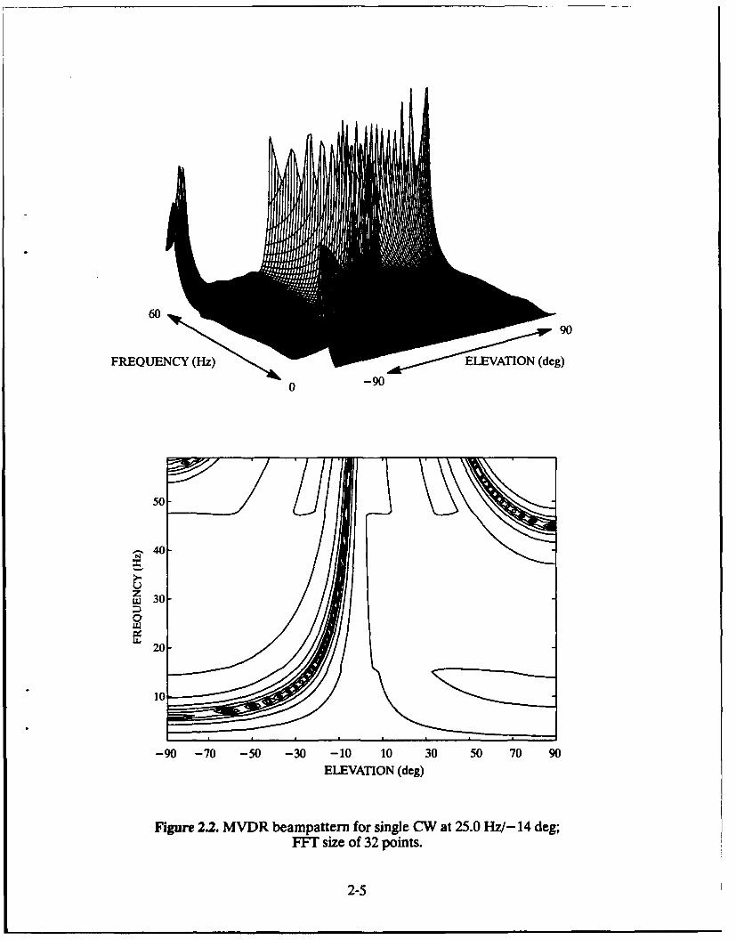
2.2. MVDR beampattern for single CW at 25.0 lHz/- 14 deg; FFT size of 32 points ... 2-5

2.3. MVDR beampattern for single CW at 25.0 Hz/- 14 deg; FFT size of

1024 points ........................................................... 2-6

2.4. Array pattern for 5-element ULA pointed at - 14 degrees .................... 2-7

2.5. MVDR beampattern for single broadband signal incident at - 14 deg; FFT size of1024 points ........................................................... 2-8

2.6. Adaptive array for narrowband signals (data and weights complex) ............. 2-9

2.7. Adaptive array for broadband signals (data and weights complex) .............. 2-9

2.8. Effects of a single discontinuity in the propagation medium .................. 2-10

2.9. Effects of a single discontinuity in the propagation medium .................. 2-11

2.10 Channel impulse response and transfer function ........................... 2-13

2.11. Inverse channel impulse response and transfer function ..................... 2-14

3.1. Continuous time time-domain conventional beamforming .................... 3-1

3.2. Discrete time time-domain conventional beamforming ....................... 3-3

3.3. Prebeamforming-interpolation time-domain beamforming .................... 3-4

3.4. Data interpolation of a single element for time-domain beamforming .......... 3-4

5.1. Channel models for two sources and three elements ......................... 5-1

5.2. Multichannel adaptive filter for broadband signals .......................... 5-3

5.3. Generalized sidelobe canceller ........................................... 5-4

5.4. Generalized sidelobe canceller implementation of the linear constrained adaptivebeamformer for broadband sources [241 ................................... 5-5

5.5. Time-domain CBF with adaptive channel equalization ....................... 5-6

6.1. MATLAB generation file for first simulation ............................... 6-3

vi

6.2. TD-CBF and GSC beamforming for three narrowband sources ................ 6-4

6.3. Bartlett and MVDR beamforming summed from 5 to 45 Hz for three narrowbandsources ............................................................... 6-4

6.4. TD-CBF and GSC PSDs along -14-, 0-, and +30-degree steering directions forthree narrowband sources ............................................... 6-5

6.5. MVDR beamforming for three narrowband sources; FFT size of 1024 points .... 6-6

6.6. MVDR beamformer output for three narrowband sources along fixed steeringdirections (top) and along fixed processing frequencies (bottom) .............. 6-7

6.7. Bartlett beamforming for three narrowband sources; FFT size of 1024 points .... 6-8

6.8. Bartlett beamformer output for three narrowband sources along fixed steeringdirections (top) and along fixed processing frequencies (bottom) .............. 6-9

6.9. MATLAB generation file for second simulation ............................ 6-12

6.10. PSD of transmitted broadband source and received data from element 1 and 5.. 6-13

6.11. TD-CBF and GSC beamforming for a single multipath ..................... 6-14

6.12. Bartlett and MVDR beamforming summed from 5 to 45 Hz for a singlem ultipath ............................................................ 6-14

6.13. TD-CBF and GSC PSDs along -14- and 0-degree steering directions for a singlem ultipath ............................................................ 6-15

6.14. MVDR beamforming for a single multipath; FFT size of 1024 points .......... 6-16

6.15. MVDR beamformer output for a single multipath along fixed steering directions(top) and along fixed processing frequencies (bottom) ...................... 6-17

6.16. Bartlett beamforming for a single multipath; FFT1 size of 1024 points .......... 6-18

6.17. Bartlett beamformer output for a single multipath along fixed steering directions(top) and along fixed processing frequencies (bottom) ...................... 6-19

6.18. Multichannel adaptive filter weights for a single multipath: presteering at0 (top) and -14 (bottom) degrees [N1 =N2 = 75] ........................... 6-20

6.19. PSD of multichannel adaptive filter output for a single multipath: presteeringof 0 degrees [N1 =N2 =75] .............................................. 6-21

6.20. Weights of the multiple single-channel adaptive filter for a single multipath:presteering of 0 (top) and - 14 (bottom) degrees IN, =N2 = 75] ............... 6-22

6.21. Weights of the multiple single-channel adaptive filter for a single multipath:presteering of 0 degrees [N1 = 150, N2 =0] ................................. 6-23

vii

A.1. Block diagram of beamforming signal processing computed with MATLAB using

various sources of input data ............................................ A-2

A.2. M ATLAB code listings ................................................. A-2

B.1. Single source ULVA ................................................... B-1

B.2. ULVA pattern for 4 = 0.5, rn = 0 degrees, N = 8, fsample = ............... B-3

B.3. ULVA pattern for d = 0.5, r = 80 degrees, M = 8, fsample = ................ B-4

B.4. ULVA pattern for d= 0.5, 0 = 0 degrees, M = 8, fsampe = 250 Hz ......... B-4

B.5. ULVA pattern for = 0.5, q = 0 degrees, M = 8, fsample = 1500 Hz ........ B-5

B.6. ULVA pattern for d = 0.25, 4 = 45 degrees, M = 8, fsample =.............. B-5

B.7. ULVA pattern for d = 1.0, 4 = 45 degrees, M = 8, fcsample =................ B-6

B.8. ULVA TD-CBF averaged beampattern M = 40, d = 30.0 m,01 = 0 degrees, f, = 25 Hz, SNR1 = 0 dB, 02 = - 5 degrees,f2 = 45 Hz, SNR2 = - 5 dB, fsample = 750 Hz, 1= 2 ...................... B-6

TABLES

2.1. Direct and multipath data for the uniform linear vertical array in figure 2.9 .... 2-12

6.1. Source parameters for first simulation ..................................... 6-1

7.1. Capabilities of beamforming algorithms ................................... 7-1

viii

SYMBOLS

Ai,Ar, A' ................ magnitude of the incident, reflected, and transmitted signals

c ....................... speed of propagating wave (m/s)

d ....................... array element spacing (m)

f ....................... frequency (Hz)

M ...................... number of elements

N ....................... number of FIR filter taps or weightsP•, P ................... instantaneous array output power and average array output

power

R(1) E[ X(f) X(f)H ] ...... spatial spectral correlation matrix

R(-u) = E[ Xa(k, u') Xa(k, u-)H ] spatial-temporal correlation matrix(or steered covariance matrix)

T ...................... number of time samples

T -0) c ........... required steering delay at the x,..(t) element to look at

direction W"

j; ....................... array steering directional unit vector

W ....................... array element weight vector

Xm,(t) .................... received signal at the mnth array element(includes source, interferers, and noise)

Xa(k,u) .................. aligned (also called steered) array element data matrix

y(k,u), Y(fu) ............. time-domain array output and frequency-domain output forlook direction W"

ix

1. INTRODUCTION

The fundamental aims of an array processing system [9] are to

1. detect the presence of propagating energy

2. determine the location of the source of propagating energy

3. classify the source from its radiation waveform

The difficulty in designing signal processing algorithms to achieve these fundamental aims

resides in the nature of the propagating energy. This energy is composed of spatial and temporal

components. While joint spatial-temporal processing has been proposed in [15], for tract-

ability, the assumption is usually made that the two components are separable, i.e.,

x(t, u-) = y(t) z(u). Some sequence of temporal and spatial processing algorithms is therefore

developed to meet the design objective. A typical sequence might be (1) temporal processing

(element data conditioning, i.e., automatic gain control, low pass filter, FFT), (2) temporal

processing (time averaging to form an estimate of the spatial spectral covariance matrix), and

(3) spatial processing (narrowband beamforming). Even though in some applications the

assumption ot spatial-temporal separation might be valid (or valid enough), there are

numerous examples when such an assumption is not valid. For instance, when an attempt is

made to detect a quiet source in a multipath environment, useful information can be present in

the multipaths. However, the multipath incident energy is both spatially and temporally

different from the direct path. In such a case, to coherently add the multipaths to the direct

path signal, spatial processing cannot be separated from temporal processing.

The aim of this report is (1) to clarify the distinction between spatial and temporal

processing in array processing and (2) to introduce several array processing algorithms suitable

for real-time applications which combine both spatial an i temporal processing. These

algorithms are based on utilizing a broadband conventional time-domain beamformer

incorporating adaptive equalization. This is a preliminary report. The merits and pitfalls of

these algorithms are discussed and demonstrated in simulations in the hope of generating

ideas and improvements.

1.1. SPATIAL PROCESSING (BEAMFORMING)

Beamforming refers to spatial signal processing algorithms used to focus an array of

spatially distributed elements (also called sensors) to increase the signal-to-interference-

plus-noise ratio (SINR) over that received by a single element [1]. It can be used to accomplish

the first and second fundamental aims discussed above. Focusing is accomplished by

1-1

coherently (i.e., in-phase) summing the element outputs. Coherency is achieved by correctingf-r the appropriate phase delay in each element (created by their spatial separation) by making

reasonable assumptions about the propagating wave's characteristics. Am, a priori informa-tion, such as sound speed profiles or source range, can be used to obtain a more accurate

estimate of the phase delay between elements in sensing the propagating energy wavefront.

Beamforming can be classified in two broad categories: conventional (or nonadaptive)and adaptive. In conventional beamforming (CBF), each element output of the array isweighted, delayed, and summed to align an incident wavefront coming from a particular

direction. The resulting directivity or spatial filtering of the array is data independent; that is,

the weights and delays are predetermined constants. Adaptive beanforming, on the other

hand, adjusts its weights and delays to the observed data. For instance, a null can be steeredautomatically in the direction of a strong interferer to suppress its effects on the array output. If

sufficient observations are available, adaptive beamforming can usually outperform conven-tional beamforming in achieving its fundamental aims. Only linear adaptive algorithms will bediscussed in this text. Nonlinear adaptive algorithms, like Volterra filters or neural networks,

are left to other sources.

Figure 1.1 shows schematically one way of relating several of the more popular beam-

forAhing algorithms (see [311 for a more comprehensive comparison of frequency-do nainnarrowband beamformers). The first classifier is the domain in which the beamforming

BEAMFORMING

I INON-LINEAR LINEAR ADAPTIVE NONADAPTIVE

I IF IiI I IFREQ-DOMAIN TIME-DOMAIN FREO-DOMAIN TIME-DOMAIN

(BLOCK) (ITERATIVE) (BLOCK) (ITERATIVE)

FII I I I I

NARROWBAND NARROWBAND BROADBAND NARROWBAND BROADBANDI TIII I ItI_ I

MINIMUM LINEAR APPLE- FROST MULTI- GENERAL- FREQ- TIME-VARIANCE PREDICTION BAUM CHAN- IZED DOMAIN CBF DOMAINDISTORTION- NEL SIDELOBE (BARTLETT) CBFLESS ADAP- CANCELLER (DELAY &RESPONSE TIVE FIL- SUM)(MVDR) TER

Figure 1.1. Relationship between some popular beamforming algorithms.

1-2

algorithm is computed, frequency (via the DFT) or time. The block/iterative classifier refers to

whether the processing is computed on a block of data or with each new sample. Narrowband

beamforming searches for the direction of an incident signal with frequency equal to that at

which the processing is being performed. Broadband beamforming searches for the direction

of an incident energy source (sum of all frequencies). A signal is usually defined as narrowband

when the bandwidth of the incident sources is much less than the reciprocal of the propagation

time of the wavefront across the array. More will be said on the use of narrowband beam-

forming with broadband data in Section 2.2.

1.2. TEMPORAL PROCESSING (CHANNEL EQUALIZATION)

Temporal processing refers to any operation which can be performed on a single

channel of data, say from a single element. A channel includes everything between the trans-

mitter, i.e., the source of energy, and the receiver, i.e., a single element of an array. The

distinction between temporal processing and spatial processing is sometimes confusing

because many of the standard temporal processing techniques (anti-alias filtering,

quantization, Fourier transforms, discrete filtering, etc.) also carry over into spatial

processing. In this text, we will be primarily concerned with the temporal processing concept of

channel equalization.

Most real-world channels are nonideal in that their frequency response does not have

constant amplitude and linear phase. A channel equalizer attempts to "invert" the frequency

characteristics of the communications channel so that the frequency response of the cascaded

channel-equalizer combination is ideal [121,[161. When the channel is not known a priori or is

time varying, it must be equalized by an adaptive equalizer. An adaptive equalizer

automatically varies its impulse response in accordance with the temporai variations of the

channel characteristics.

In a multipath channel, the received signal consists of the sum of a number of individual

components that have traversed paths of differing lengths between the transmitter and the

receiver. Depending on the phase relationships between these components, they can either

add constructively or destructively at the receiver. The channel equalizer must sort out the

multipaths from the direct path and coherently recombine all components into a single output.

1.3. SIGNAL MODEL

In this text, it will be assumed that L sources (which include interferers as well as the

target source), so(t) 1 = 0, 1,2,...,L - 1, each generate a stochastic plane-wayv, signal which

1-3

propagates in an isovelocity medium through M spatially separated array elements,

Xm(t) m = 0, 1,2,...,M - 1. A -ource refers to any incident plane-wave signal; thus, a single

discrete energy source may actually generate multiple sources, a direct path plus any multi-paths due to reflected or refracted paths. The plane-wave approximation is valid in anisovelocity medium for sources located at a distance from the array equal to roughly 60 or more

times the aperture of the array (the so called "far-field" solution) [9]. An isovelocity mediumimplies that a wave travels at the same speed of propagation throughout all space. Note that a

far-field source can generate a curved wavefront in a multivelocity medium (see [40] or [18]). Itis assumed in this text that the speed of propagation and the exact element location is known.

Each source sAt) produces a plane-wave response at the xm(t) element equal toXm~) s~t •' Xm

Xm) = + * ) + flm(t) (1.1)

where

im - position vector for the xm(t) element

= negative directional unit vector for the sAt) source

C = speed of propagation of the acoustic plane wave

nm(t) = noise at the xm(t) element (assumed to be spatially uncorrelated)

is the difference between the arrival time of the plane wave from s1(t) at the mth

element, xm(t), and the arrival time of the same wave at the origin. Thus, for i',,, 1 •T or

,m = (0, 0, 0), this time difference will be zero. Figure 1.2 displays the coordinate system usedthroughout this text.

SX = ELEVATIONX -ANGLE

(+DOWN, - UP)0 = AZIMUTH ANGLE

(OR BEARING)y r (0 - NORTH)

x = rcosocos0I z (X, y, Z) y = r cosp sin0

z = r sino

Figure 1.2. Coordinate system.

1-4

2. GENERAL BEAMFORMING ISSUES

This section discusses several adaptive beamforming issues relevant to the develop-

ment of the beamforming structures in Section 5. In particular, it briefly discusses the

performance of the adaptive array with respect to the number of elements, the signal band-

width, and a multipath environment.

2.1.PERFORMANCE VERSUS ARRAY SIZE

Array gain is the improvement in the SINR due to beamforming. One definition

commonly used is [9]

array gain = SiNRinput (2.1)

(in Ch. 4.2.4 of [9], the noise term implies interferers plus noise as explicitly stated here; seealso [8],[11]). Note that if a large interferer is cancelled by a beamformer, the array gain givenby Eq. (2.1) can be quite large. The array gain at the output of an ideal M element array for the

case of no interferers and spatially white, isotropic noise is equal toarray gain = 10 logl 0(M) dB (2.2)

regardless of the arrival direction (see, for example, p. 37 of [11]). As the interference-to-noise

ratio (INR) increases, however, the array gain will change depending on (among other things)the number of interferers, the direction of each interferer, and the power in each interferer.For instance, if a 10-element array effectively cancels a 30-dB interferer, then the array gain

given by Eq. (2.1) can be as large as 40 dB [= 10 log(10) dB + 30 dB]. For more on array gain

see [5].

Any adaptive array with M independently controlled elements has M degrees of

freedom, which are typically distributed as

M = [no. of constraints] +[no. of steer directions] + [no. of interference nulls] (2.3)

For example, the minimum variance distortionless response (MVDR) has I constraint of

constant magnitude in the single steer direction and so has a capability of generating M-2interference nulls in its array response. When more interferers are incident on an array thanthe array is capable of cancelling, the adaptive weights will collapse (to zero) as the incident

INRs increase and the array gain will deteriorate [8].

2.2. EFFECTS OF SOURCE SIGNAL BANDWIDTH

Broadband signals create (at least) three separate problems in array processing. The

first deals with the fact that the interelement phase shift is a function of frequency. To see this,

consider the interelement phase shift for a broadband signal

inter - element phase shift = 2 ;r f [Tm(U) - r, 1(5)

2-1

where Tm..(u-i) =•x' "m u is the time it takes a plane-wave coming from direction W" to propagatec

from the xm(t) element to the origin. The interelement phase shift is seen to be linearlydependent on the frequency of the signal. We can investigate the ramifications of thisdependence further by considering the uniform linear array (ULA) with element spacing d.For this case and a signal incident to the array from angle r, we find

inter - element phase shift = 2 ar f sin( Q)] (ULA) (2.4)

From Eq. (2.4), it is apparent that a single signal withfsource arriving from angle 4 ~source can be

perceived by the array as having a different frequency content, fArray, and arriving from a

different angle, aray, as long as the interelement phase shift is unchanged, or

farray sin(4array) = fsource sin(4?source). This can happen in narrowband beamforming when-

ever farray ; source. In these cases, the source appears to be incident from an angleI. = sin-1 [ r-- sin(osource) (ULA) (2.5)

ara Lfsource I

For narrowband frequency-domain beamforming, two situations can arise where

faray d fsource: (1) when the temporal DFT performed on each element's time data is not of

adequate size so that spectral leakage between frequency bins is significant, and (2) when thespatial spectral correlation matrix, R(f), and the steering vector, E(f2,ii) (defined in Section4), are formed at different frequencies.

Figure 2.1 demonstrates the effect of an inadequate size of temporal FFT, with the

MVDR adaptive beamformer processed at 15.625 Hz (bin centered for a 1024-point FFT).

The incident signal on the 5-element vertical ULA with d=30-m spacing is a narrowbandsignal at 25.0 Hz coming in at - 14 degrees (c= 1500 m/s) and sampled at 1000 Hz (all examplesin this text are sampled at 1000 Hz). One would expect the MVDR processor to yield zero

output when processing is done at any frequency other than 25.0 Hz. However, figure 2.1 showsthat for FFT sizes of 32, 64, and 256 points, the spectral leakage from the 25.0-Hz source into

the 15.625-Hz bin creates an apparent arrival angle of -22.8 degrees, as described by Eq. (25).As the frequency bin leakage is decreased with larger FFTs, the desired solution is obtained. In

figure 2.2, the MVDR beampattern* is plotted for the same vertical ULA and 25.0 Hz source

for farray = 1, 2,3,..., 60 Hz. An FFT size of 32 points was used to clearly illuminate the arc sin

dependence of Eq. (2.5) (clearly farray fsource ). Figure 2.3 plots the MVDR beampattern

results for an FFT size of 1024 (with 50% overlap). The figure shows the correct frequency and

* The beampattern is defined in this report as the array's output energy (f P, -u) df ) as the direction oflook is varied. It is a real valued quantity. J

2-2

0

-10-

•" 20-

/" . 32-PT FFT

64-PT FFTI.~-30-

091.

-40 ...............

5256-PT FFT-50

.- '--. - 1024-PT FFI-- _---------... . .-.--- - --.... / ..................

-606-100 -80 -60 -40 -20 0 20 40 60 80 100

ELEVATION (deg)

Figure 2.1. MVDR beampattern for single CW at 25.0 Hz/- 14 deg;FF1T sizes of 32, 64, 256, and 1024 points.

angle of the incident signal. Unless otherwise stated, a 1024-point FFT with 50% overlap will

be used in all narrowband frequency-domain beamforming.

The second problem associated with broadband signals is spatial aliasing, which creates

a directional ambiguity in the beampattern. Expressions for spatial aliasing are based on the

sampling theorem NO TAG and are a function of the incident angle of the signals. The worst

case for spatial aliasing in the ULA with element spacingd is when the incident angle is +/- 90

degrees (end-fire). Under these conditions, spatial aliasing will occur when

_d <C 1 1 (2.6)j 2 fMAx

wherefMAX is the largest temporal frequency of the incident signals. The best case for spatial

aliasing in the ULA with element spacing d is when the incident angle is 0 degrees (broadside),

where spatial aliasing will occur whenever

d<= 1C fMA (2.7)

In the previous example, d = 30 m, c = 1500 m/s; we can expect the onset of spatial aliasing to

appear when the frequency of the incident signal is between 25.0 Hz and 50.0 Hz, depending onthe incident angle of the signal (see Appendix B for more discussion on grating lobes andtime-domain conventional beamforming (TD-CBF) with a ULA). Spatial aliasing can beviewed clearly as grating lobes in the array pattern.* The grating lobes can be clearly seen infigure 2.4, where the array pattern of the 5-element vertical ULA is plotted for a steer direction* The array pattern is defined in this report as the complex valued weighting given to an incident signal as its

direction is varied when the array's direction of look is fixed. For equally spaced elements, it reduces to thesioatial Fourier transform of the array wei2hts.

2-3

of - 14 degrees. Figure 2.4 is plotted from - 180 degrees to + 180 degrees for a complete viewof the grating lobe structure. Note that because the array is linear along the Z axis, its array

pattern is azimuthally independent. Thus, the array pattern actually forms a main cone and a

grating cone when Eq. (2.6) is satisfied. It is straightforward to show that the true angle (versusthat defined by the grating lobes) forf > 1/2fpf.4 lies between

si21[ fsorce d] 2 inI[ fsource (2.8

Figure 2.5 plots the MVDR beampattern for a broadband signal incident on the 5-element

vertical ULA from - 14 degrees. The grating lobes are readily apparent for f > 40 Hz.

The last problem associated with broadband signals is that the array pattern's mainbeam width is a function of frequency (as well as a function of the steer direction). This can also

be seen in figure 2.4, where the main beam gets wider at lower frequencies, and thus theresolvability between two closely spaced sources becomes more difficult at lower frequencies.

A closed-form approximation for the main beam width of a uniform linear array is found in

Appendix B. Broadband beamformers which integrate across frequencies (either implicitly or

explicitly) will have to take this issue into effect, especially if significant amounts of energy exist

at the lower frequencies. The simplest method is to filter out the low frequencies (as well as thehigh frequencies for reducing spatial aliasing) to retain the required beam width for adequate

resolution.

2-4

6090

FREQUENCY (Hz) ELEVATION (deg)

0 -90

50

, 40-

z

z 30

019.

S20o

10

-90 -70 -50 -30 -10 10 30 50 70 90ELEVATION (deg)

Figure 2.2. MVDR beampattern for single CW at 25.0 Hz/- 14 deg;

FFT size of 32 points.

2-5

60

90

FREQUENCY (Hz) ELEVATION (deg)

0 -90

...... N .o

02-

60S~180

FREQUENCY (Hz) ELEVATION (deg)

0 -180

50

w

-180 -130 -80 -30 30 80 130 180

ELEVATION (deg)

Figure 2.4. Array pattern for 5-element ULA pointed at - 14 degrees.

2-7

60S~90

FREQUENCY (Hz)

ELEVATION (deg)0 -90

50

40

z 30-

10- -

-90 -70 -50 -30 -10 10 30 50 70 90ELEVATION (deg)

Figure 2.5. MVDR beampattern for single broadband signal incident at -14 deg;FF1 size of 1024 points.

2-8

This section has introduced some of the effects of signal bandwidth on spatial pro-

cessing. Insight here is crucial to understanding the beampattern output and the operation of

various beamformers. Figures 2.6 and 2.7 show simplified adaptive arrays for narrowband

signals and broadband signals, respectively [28]. A single complex weight is capable of

supplying the required gain and phase adjustment at each element for narrowband signals, as

seen in figure 2.6. The tapped-delay line in figure 2.7 permits the adjustment of the gain and

phase at a number of different temporal frequencies, as required for the array processing of

broadband signals. Signal preconditioning has been left off both figures for clarity.

xl(,)_• • 0'• yt' U)Xo(t)

/

Figure 2.6. Adaptive array for narrowband signals (data and weights complex).

XM_1(t)1Z-

X@00

0001(t -U

Figure 2.7. Adaptive array for broadband signals (data and weights complex).

2-9

2.3. SOURCE-TO-ELEMENT PROPAGATION CHANNEL

Two identities from ray theory can be used to generate a more complete picture of the

source (including interferences) to element propagation channel in a nonhomogeneous

medium. Consider figure 2.8 where an incident wave is colliding with a single abrupt

discontinuity. We find that [7]

1. Incident angle is equal to the negative of the reflected angle

Oi = -Or (2.9)2. Snell's Law:

cos(])i - cos(o)t)Cl C2 (2.10)

where cI and c2 are the speed of propagation of a plane wave in medium 1 and medium 2,

respectively. From Eq. (2.10) it can be seen that there exists a critical incident angle where if

0i <- c, no transmission results. The critical angle is

(= cos-(C) (2.11)

The ratio of the sound speeds in the two mediums, L' is called the index of refraction.C2 '

REFRACTED (TRANSM1TTEDWITH CHANGE IN DIRECTION)

Z2 ~L

Z, O/r j

Z2 > ZI REFLECTED INCIDENT Z

Figure 2.8. Effects of a single discontinuity in the propagation medium.

The magnitude of the reflected and transmitted waves depends on the characteristic

acoustic impedance, Z = L c, where @ is the medium density. For instance, it is straight-forward to show that the magnitude of the reflected wave is related to the magnitude of theincident wave by [7]

[z2 sin(¢i) - z1 lfi(9¢,)]1Ar = A' Z2 sin*i) + Z1 sin((t) (2.12)

and that the magnitude of the transmitted wave is [7]

At = A' 2 2 sn('Oi (2.13)Z2 sn -10 sin(ol)

2-10

Using Eq. (2.9)-(2.13), we can compute the magnitude and direction of the reflectedand transmitted waves. For example, assume that a source is 2000 m from a uniform linearvertical array and 250 m from an abrupt impedance boundary, with Z 2 = 1.5/1.45 Z1 = 1.035Z1, as shown in figure 2.9. Table 2.1 summarizes the multipath and direct path data for variouselement depths. The data show quite clearly that the magnitude of the multipath, Ar, isdifferent for many of the elements. For a large array, each element will most likely see adifferent propagation channel. In fact, it is possible for an element to see no signal, direct ormultipath, from the source or to see only a transmitted multipath and no direct path (see, forinstance, the top two elements in Z 2 in figure 2.9). Thus, for an algorithm to use the multipathinformation to increase the array gain, each signal-to-element channel must be treatedindividually.

The underlying difficulty with including the multipath data is that it is temporallydelayed and deformed (due to nonideal propagation such as spreading, absorption, ductingand nonideal boundary interactions) as well as spatially different from the direct path. Mostadaptive beamformers treat incident energy which is spatially different from the steerdirection as interference to be nulled out. This is equivalent to making the implicit assumptionof all source-to-element propagation channels being equal and no multipaths existing.

A t

NO TRANSMISSION

-

X Ai

Z2= 1.035 Z1Zcz = 1450 rn/s

Figure 2.9. Effects of a single discontinuity in the propagation medium.

2-11

Table. 2.1. Direct and multipath data for the uniform linear vertical array in figure 2.9.

Element Ar 01 4 = 4- x Reflect Direct Multi- DiffDepth (m) (deg) (deg) (m) Path (m) Path (m) (ms)

190 1.0 - 12.4 863 2000.9 2047.8 32.3

220 1.0 13.2 936 2000.2 2054.5 37.4

250 1.0 - 14.1 1000 2000.0 2061.6 42.5

280 0.94 0.5 14.8 1056 2000.2 2069.6 48.0

310 0.52 5.0 15.6 1107 2000.9 2076.9 53.0

340 0.4 7.2 16.4 1153 2002.0 2085.2 58.7

370 0.33 8.9 17.2 1194 2003.6 2093.9 64.8

2.4. SOURCE-TO-ELEMENT PROPAGATION CHANNEL MODEL

Each source-to-element propagation channel can be modeled as a FIR filter with

impulse response

..m(n) = 6(n - nd•'eet) + Ar,i 6(n - ru)(2.14)i=1I

for the mth element and I multipaths [12]. By aligning the received element data to point

towards the direct path, we have a channel impulse response

Ihm(n) = 6(n) + r Ar 6(n - nmý-t + ndrect)

i=I

= 6(n) + 3 Arm~ 6(n - 0 2.5

We can take the Z transform of Eq. (2.15) for a single multipath (I=1) to find the channel

transfer function between the source and the mth element

Hm(z) = ihm(n) z-= 1 +Am (2.16)n=O

The power spectral density of the mth element is now related to the power spectral

density of the source by

PSDx.(I) = IHm(f)2 PSD&() (2.17)

where

2~~~1 1+ +r 2 r0H,() + (Ar)2 +2Am cos(2 ;r f n°) (2.18)

The spectral nulls in Eq. (2.18) are characteristic of a multipath channel and can be seen in

figure 2.10 forAm r= 0.8, and nm 0 = 5. It is seen from Eq. (2.18) that the depth of the spectral

2-12

CHANNEL IMPULSE RESPONSE CHANNEL TRANSFER FUNCTION

1.00

0.6- -2-0.4-

S0.2 -4-

"• -0.2-

-042 ---0.4-

--0.6- -8-.0.8-

-1, -10,0 5 10 15 20 0 fs12

TIME DELAY NORMALIZED FREQUENCY

Figure 2.10. Channel impulse response and transfer function.

null in the channel's transfer function increases with the amplitude of the multipath (Amr) and

that the distance between spectral nulls decreases as the delay (nn 0) between the direct and

multipaths increases.

2.5. SOURCE-TO-ELEMENT PROPAGATION CHANNEL EQUALIZATION

Even though the multipath can be distorted by the propagation channel and arrives atthe array from a direction other than that of the direct path, it contains energy coherent with

the signal of interest. If each source-to-element channel can be equalized, i.e., the effects of the

multipath are negated, then the SINR of each element and thus the array can be enhanced. (It

should be noted that two broadband signals are fully correlated if they are amplitude-scaled

and temporally delayed replicas, while two narrowband signals are fully correlated if they have

a fixed phase difference relative to each other. Multipath signals are usually partially

correlated to the direct path due to nonideal reflections or Azfractions.)

Continuing under the premise that the inverse filter can be found, we can find that thetransfer function of the ideal equalizer or inverse filter is

S~1HZ) = Hm(Z) (2.19)

For the single multipath example above00

._ Z(_ Ar)i z-nO,.iHM(z) = +Arm z- _ Am, (2.20)M i=O

using the geometric series. Thus, the ideal inverse filter impulse response is

h'nv(n) = (-- Armin,, for i = 0, ne, 2nom,...

h`V(n) = 0 otherwise (2.21)

2-13

Note that hm inV(n) is stable if and only if lAm r I < 1. Figure 2.11 plots the first 20 taps of theideal inverse channel impulse response (Eq. (2.21)) and the ideal channel transfer function. Itis apparent from comparing figures 2.10 and 2.11 that the cascaded channel-inverse filterresults in a distortionless transmission albeit delayed in time. This is the aim of channelequalization.

INVERSE CHANNEL INVERSE CHANNELIMPULSE RESPONSE TRANSFER FUNCTION

1.0 00.8-

0.6- -2-

0.4-

- 0.2- -4-

"'• -0.0 SS-0.2- -6-

-0.4-

-0.6- .8--0.8-

-1 -10-0 5 10 15 20 0 fs12

TIME DELAY NORMALIZED FREQUENCY

Figure 2.11. Inverse channel impulse response and transfer function.

2-14

3. TIME-DOMAIN BEAMFORMING

Time-domain beamforming techniques are used in communication, in transient signal

analysis, or for wideband sources. This section briefly introduces time-domain beamforming

and its discrete implementation. It introduces notation and concepts used later in this text.

3.1. CONTINUOUS TIME-DOMAIN CBF

To coherently add the outputs of all elements in the time-domain requires the proper

delay of each element before summing. The delay is determined by the desired "steer" (or"look") direction. The summation can be written as

M-1

y(t,u-) = W! X.(t - T.(U-) (3.1)m=O

where

i7 = steering directional unit vector for the (0, 0)th direction

Tm =xmcU = required steering delay at the xm(t) element to look at direction W

Wm = weight (or shading coefficient) for the Xm(t) element

Figure 3.1 is a direct implementation of Eq. (3.1). It represents pure spatial processing, since

the temporal delay operation has a distortionless transfer function (constant amplitude and

linear phase).

SDRCTOXM-,1(t) T •M-

STEER DIRECTION

X 0(t) CM

wX W,-.-Ayt, ýU

XxWO

Figure 3.1. Continuous time time-domain conventional beamforming.

The instantaneous power in the beamformer output, Py(t, u-) = Vt, --)I2 will display a

peak whenever the steer direction equals a source direction. (Recall that

Ly(t, u)12 = y(t, u) y*(t, u-), where y(t, u-) is the complex conjugate of y(t,u-i).) In low SNR

3-1

environments, Py(t, -u) must be time-averaged to adequately resolve a source direction. Since

Eq. (3.1) is a summation of all energy coming from a particular steer direction, it can be used to

detect broadband sources as well as narrowband sources. To classify the source, the spectrum

of the beamformer output must be analyzed.

3.2. DISCRETE IMPLEMENTATION OF TIME-DOMAIN CBF

To implement any algorithm in hardware requires that the continuous input data be

sampled so that t -- k A t, where k is a positive integer and A t = 1 is the sampling interval.

Sampling Eq. (3.1) and normalizing each iteration to the sampling interval At, we find the

beamformer output can be written as

y(k, u-) = WH Xa(k, u-) (3.2)where W is the Mxl weight vector

WT = [Wo,Wl,W 2 ,...,WM-l] (3.3)

and Xa(k,ui) is the Mxl perfectly aligned data element vector (or snapshot) at time kXa(k,u-)T - [xo(k - ro(u•)), xl(k - T-u-)), x 2(k - -2(u-))' ... , xM. (k -- TMM_(U))]

= [Lx(k), x(k), x2(k), ... , xl(k)j (3.4)

The alignment of the element data essentially creates a broadside steer direction. With these

vectors defined, the instantaneous power in the beamformer output can be rewritten as

Pi(k, 5) = y(k,i) y*(k,iu-) = WH Xa(ku-5) Xa(k,u5)H W (3.5)

Figure 3.2 shows the new TD-CBF structure and notation. From the figure it can be seen that

time-domain CBF is very simple to implement. Simply retain a time-history of each element's

input data, and then sum the properly delayed data from each element in the array. The

average power output is found by taking the expectation of both sides of Eq. (3.5) to givePy(u-) = WH R(u-Q) W (3.6)

where

R(-u) = E[ Xa(k, _u) X"(k, u-)H] (3.7)

is the spatial temporal correlation matrix [9] (also called the steered covariance matrix in [41]).

If the input process is ergodic, then a time average will approach Eq. (3.6) (see, for example,

Ch. 2 of [14]).

Unfortunately, the element delays are rounded to the nearest integer in the discrete

implementation. Thus, the discrete time element delays are given by

3-2

Tm(-u) = round[m CSI- u ]c fs (3.8)

where round[x] rounds x to the nearest integer. (The round operation is inherent in the

sampling process.) It is apparent from Eq. (3.8) that the steering delays will be rounded to

integer multiples of the sampling period. Thus, the higher the sampling frequency, the moresteer directions are possible and the better the delineation of the array beam pattern.

x.. .(k. ,-, , xM - I (k)

WM-1

xl(k) xak 0W1 k

y(k, u-)

x0(k) - Z To X a k (

wo

Figure 3.2. Discrete time time-domain conventional beamforming.

Often interpolation is required to obtain the desired delineation of the array pattern.

Two possible techniques for data interpolation are (1) conventional time series interpolation,

which effectively resamples each element's data at a higher sampling rate [9] and (2) data

interpolation by a linear 2-tap FIR filter or a quadratic 3-tap FIR filter to interpolate between

data values while retaining the same sampling rate (see, for example, Ch. 3.1 of [4]).

Figure 3.3 shows the most intuitive means of implementing conventional interpolation,

called low-pass prebeamforming interpolation [26]. Each element is resampled at a higher

sampling frequency, allowing for more precise control over the steering delays. Enough data

memory from each element must be retained to account for +/- maximum steer delay (in

number of samples), which is a function of the resampled sampling frequency, the speed of

propagation, the element location (with respect to the origin), and the steer direction. When

the number of steer directions is greater than the number of array elements, a computationally

more efficient method of interpolation can be used, called low-pass postbeamforming

interpolation [26]. The interpolation operation can be separated into two operations: (1) -1

3-3

zeros added between each successive data sample and (2) interpolation filtering. I determines

the amount of interpolation and is assumed to be an integer greater than 1. In postbeam-

forming interpolation, the zero adding is done before the delay and sum beamforming com-

putation, while the interpolation filtering is performed after the delay and sum beamforming.

Both techniques result in similar improvements in determining the angle of arrival of the

source.

O-*'- I Q) SHx 10t) [ -[ - ' ] x I(k) "- - - - - 2 . D EC] POW ER OVER

S/ D*l*f,

DIRECTION

Figure 3.3. Prebeamforming-Interpolation time-domain beamforming.

A second method of data interpolation which does not increase the data rate is shown in

figure 3.4 for a single element. First, the rounded-down integer delay is used for coarse data

alignment. Then a small FIR interpolation filter (either 2 taps for a linear interpolation or 3

taps for a quadratic interpolation) is used to compensate for the difference between the actual

delay and the rounded-down integer delay. Essentially, the interpolation filter provides for

fine steering. In most cases, the generation of the aligned data matrix will require some method

of data interpolation for adequate beampattern delineation.

Xm*,()

DATA ALIGNMENT INTERPOLATION FILTER(COARSE STEERING) (FINE STEERING)

Figure 3.4. Data ;nterpolation of a single element for time-domain beamforming.

3-4

4. FREQUENCY-DOMAIN BEAMFORMING

Frequency-domain spatial processing is an especially efficient technique when the

stochastic signals are narrowband and sustained rather than transient [9]. This section briefly

introduces two of the more popular frequency-domain beamformers, Bartlett and MVDR.

References are provided for more detailed information.

4.1. FREQUENCY-DOMAIN CBF (BARTLETT)

The array output can be analyzed in the frequency domain as well as the time domain.

In the frequency domain, time-delays transform into frequency-dependent phase shifts. Thus,

taking the Fourier Transform of Eq. (3.1), we obtain

gF{y(t, I = r W! Xm(t - rm.(U))}

M-1Y(f, U- = I" w e-Jnr(a t( (4-1)

m=0where Xm0f) is the single element (also called along-channel) temporal Discrete Fourier

Transform of xm(t) in a discrete implementation. Eq. (4.1) can be rewritten in terms of linear

matrixes

Y(f, u-) =E(f,)H WH X(j) (4.2)where

E(f,iu))r= [e+i2frf('), e+j 2 nfi(') , ... , e+i2 nfTMI(-)] (4.3)WT= diag[wo, wl, ... , WM_1] (4.4)X0p)r= [X00') , XlJ) .. XN_I(]] (4-5)

E(f, ) is the plane-wave steering vector which corrects for the phase delays at frequencyf

between elements when the array is steered in direction _u. The FFTs are usually performed

with a 50%- 75% overlap, weighted with a good FFT window (e.g., the Hanning window), and

are of an adequate length (e.g., 1024-8192) for good frequency resolution NO TAG. Padding

the along-channel data with zeros for good frequency resolution is equivalent to the data inter-

polation discussed in the previous section. WT is a diagonal matrix containing the element

weights (shading coefficients). For unity shading, WT reduces to the identity and can be

dropped out of the equations. The instantaneous power in the array output is given by

P;,[f, u-) = Y(f, -u) Y*(f, u-) = E(f, u)H Wt/ X(b) X(f)H W E(f, u-) (4.6)Or taking the expected value of both sides, we find the average power output as

4-1

Py(fu) = E(f, )H WH RQ) W E(f,u) (4.7)where

R) = E[ X() X()H]

is the spatial spectral correlation matrix NO TAG (also called the cross-spectral density matrix

[61). In practice, only an estimate of R(j) can be computed:

N

R(J) -Rh =1ZX0 XOQH (4.8)iN l

The efficiency of Eq. (4.7) is that once an estimate of R(f) is formed, any new direction

can be searched by simply generating a new plane-wave steering vector, E(f). For broadband

signals, Eq. (4.7) is computed for multiple frequencies within the band of interest and then

summed across frequency.

4.2. MVDR

MVDR is an example of a linearly constrained adaptive beamforming algorithm. It has

the ability to adapt to the spatial interferer environment and place spatial nulls wherever

strong interferers exist. The MVDR method determines the weight vector, W(f,'), which

minimizes the average array output power:

P'fu-) = W(f,u-)H R(f) W(fu) (4.9)

subject to the constraint that the steer direction has distortionless response (constant

amplitude and linear phase), i.e., W~f, uH) E(f, -u) = 1. It was shown in [9] (see also [31]- [401

for more on MVDR) that the array element weight vector satisfying these constraints is

W(f, U-)= R(f) -I E(f,u) (4.10)

E(f,u-)H R)-I E(f,il)

Using Eq. (4.10) in Eq. (4.9), we find the average output power to be

P ,0=1 (4.11)PY~f'• E(f, u-)H ROf)- In(f,u-') (.1

Once an estimate of R(Q) is formed, its inverse must be computed. This requires O(M3 )

operations in general and can be a numerically unstable operation if the condition number of

R(f) is large. However, once this inverse is computed, any direction can be searched by just

generating a new plane-wave steering vector, E(f). Since the spectra of MVDR are constrained

in the direction of look and because of the narrowband processing, MVDR is not capable of

channel equalization.

4-2

5. BROADBAND BEAMFORMING INCORPORATINGADAPTIVE EQUALIZATION

This section discusses adaptive beamforming algorithms capable of channel

equalization. The complexity of the underlying problem is depicted in figure 5.1 and is

described in more depth in [13] and [15]. Each source signal is convolved with its local source

impulse response (transducer, ship hull, etc.), S1(z), before being transmitted into the prop-

agation medium. As described in Sections 2.4. and 2.5, each source-to-element is modeled as a

separate transmission channel (which includes multipaths, distortion, propagation losses,

etc.), Hij(z). Upon reception at each array element, the receiving data undergo another

convolution with the element's impulse response (transducer), Ej (z). To simplify the problem,

it will be assumed that each element is equalized and that the problem is to equalize the

channel such that si (t) is recovered. The channel models are assumed to be linear and slowly

time varying.CHANNEL MODELS

SOURCE MODEL ELEMENT MODEL- t) ELEMENT I

SOURCE1 1It

ELEMENT MODEL

CHANNEL M 2Z 0

SOURCE MODEL LEM LEMENT MODEL

SOURCE 220

**S 2(Z) EZ

TRANSMITING PROPAGATION MEDIUM RECEIVNGSOURCES (MODELS DEPEND ON SOURCE ARRAY

AND ELEMENT LOCATIONS)

Figure 5.1. Channel models for two sources and three elements.

5-1

5.1. MULTICHANNEL ADAPTIVE FILTERING

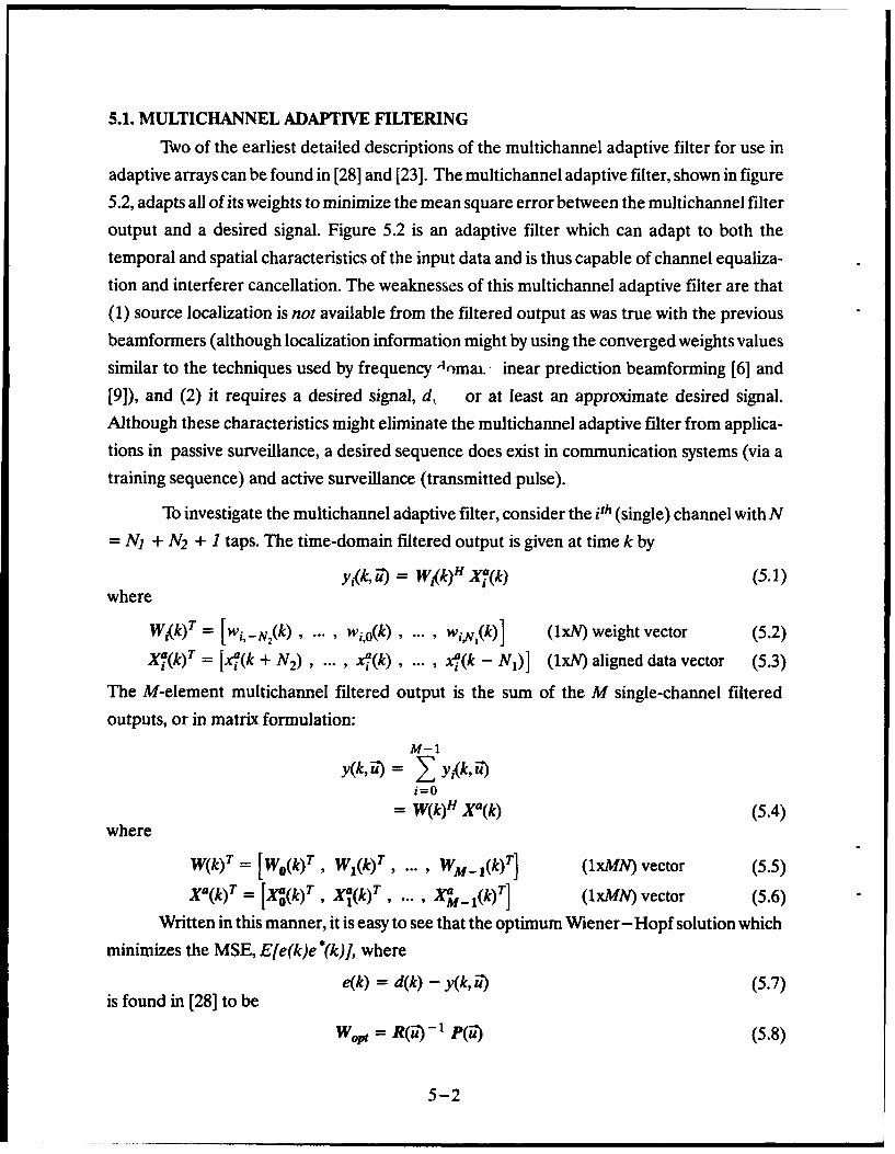
Two of the earliest detailed descriptions of the multichannel adaptive filter for use in

adaptive arrays can be found in [28] and [231. The multichannel adaptive filter, shown in figure

5.2, adapts all of its weights to minimize the mean square error between the multichannel filter

output and a desired signal. Figure 5.2 is an adaptive filter which can adapt to both the

temporal and spatial characteristics of the input data and is thus capable of channel equaliza-

tion and interferer cancellation. The weaknesses of this multichannel adaptive filter are that

(1) source localization is not available from the filtered output as was true with the previous

beamformers (although localization information might by using the converged weights values

similar to the techniques used by frequency "4omai. inear prediction beamforming [6] and

[9]), and (2) it requires a desired signal, d, or at least an approximate desired signal.

Although these characteristics might eliminate the multichannel adaptive filter from applica-

tions in passive surveillance, a desired sequence does exist in communication systems (via a

training sequence) and active surveillance (transmitted pulse).

To investigate the multichannel adaptive filter, consider the Pth (single) channel with N

= N1 + N2 + 1 taps. The time-domain filtered output is given at time k by

y,<k, -)= W,(k)H Xi(k) (5.1)where

wxk)T= [wi,_.N,(k) , w..., W,(k) , ... , W,(k)] (lxN) weight vector (5.2)

Xi(k)T = [xia(k + N 2), ... , xi(k), ... , xfi(k - N 1)] (lxN) aligned data vector (5.3)

The M-element multichannel filtered output is the sum of the M single-channel filtered

outputs, or in matrix formulation:

M-1y (k,-u-) y A yk,-u-)

i=O- W(k)H X*(k) (5.4)

where

W(k)T [W 0(k)T, W,(k)T, ... , W_,1 (k)T] (lxMN) vector (5.5)

= [X•(k)T, X(k)T, ... , X 1_,(k)T] (lxMN) vector (5.6)

Written in this manner, it is easy to see that the optimum Wiener-Hopf solution which

minimizes the MSE, E[e(k)e *(k)], where

e(k) = d(k) - y(k, u-) (5.7)is found in [28] to be

Wopt = R(-u) -I P(i') (5.8)

5-2

or in [14] for detailed single-channel adaptive filter theory. In Eq. (5.8), R(u-) is the multi-

channel, spatial temporal correlation matrix and P(Q) is the multichannel, cross-correlation

matrix given by

R~u) = E[ Xa(k) Xa(k)H] (MNxMN) vector (5.9)

Pu) = E[ Xa(k) d'(k)] (MNxl) vector (5.10)

Numerous methods of solving Eq. (5.8) without actually inverting the MNxMN matrix

(which requires O(M 3N3) operations in general) have been explored in the past 30 years. The

recursive least squares (RLS) solution (also called Kalman Filter) requires O(M2N2 )

operations [22]. While the shifting property does not exist between channels as would be

required for (super) fast RLS solutions (i.e., O(MN)), it does exist within a single channel, as

shown in figure 5.2. This property has been exploited by [19] and [25] to derive two different

multichannel RLS lattice algorithms with O(M2N). The application of stochastic solutions like

least mean squares (LMS) to the problem does not require matrix inversions. This results in

O(MN) algorithms, but the performance of these algorithms is dependent on the data [28].

xM,_1l(k) 0 -m _' XMI(k + N,) xu_ (k) xm-_ (k - NI)

WM-1.-N2 *** - ' OSWMI'

x1 (k) xw,(k + N2) ) .r-N)yMl(k,iWK-I.-Arz 000 WM ' * 0 W -I.

x1(k) Z-T1 X00 k + NN,2 -1xak) Z1x 0 a(k N- N\ )ym1ku

x+ ekk

Wl,-N 000 Wi' *s • N k_)yk

SX'a k + N, /'a X

xO~) -T 2 Z 1d~ ak) Z 1 ( , k u ) e(k

Figure 5.2. Multichannel adaptive filter for broadband signals.

The data alignment helps to minimize the required length of the single-channel FIR

filter, N. By interpreting Eq. (3.8), we see that the length of the filter N (as well as other

parameters) determines the possible steering delays, which in turn determine the angles at

5-3

which the multipath can arrive and still be equalized. Thus, by aligning the data toward aparticular direction, a range of angles is defined for which the filter can equalize multipaths.For example, the uniform linear array with M elements can equalize multipaths as long as theyarrive within - sin-1[2V2 C 1 <q5 < +sin-2 - c 1 iI degrees of the

steered direction, W.

However, since the adaptation is based on minimizing the output error power, if thesame desired sequence is used for all steer directions, the weights will always attempt toequalize the same signal (as long as it is in the range of possible angles defined byN above). Thegeneralized sidelobe canceller to be discussed in the next section will modify figure 5.2 to use aTD-CBF to generate the desired signal. It is dependent on the steer direction and will thusprovide more directionality information.

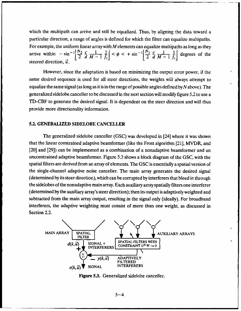
5.2. GENERALIZED SIDELOBE CANCELLER

The generalized sidelobe canceller (GSC) was developed in [24] where it was shownthat the linear constrained adaptive beamformer (like the Frost algorithm [21], MVDR, and[20] and [29]) can be implemented as a combination of a nonadaptive beamformer and anunconstrained adaptive beamformer. Figure 5.3 shows a block diagram of the GSC, with thespatial filters are derived from an array of elements. The GSC is essentially a spatial version ofthe single-channel adaptive noise canceller. The main array generates the desired signal(determined by its steer direction), which can be corrupted by interferers that bleed in throughthe sidelobes of the nonadaptive main array. Each auxiliary array spatially filters one interferer(determined by the auxiliary array's steer direction); then its output is adaptively weighted andsubtracted from the main array output, resulting in the signal only (ideally). For broadbandinterferers, the adaptive weighting must consist of more than one weight, as discussed inSection 2.2.

MAIN ARRAY SPATIAL AUXILIARY ARRAYSFILTER ]W X • V

"• ....... ISPATIAL FILTERS WITHd(k'u)+ F INTERFERERS CONSTRAINT UHW~-0

'i( I \(xi)_ y(k, u-) ADAPTIVELY

FILTERED

e(k, u-) SIGNAL INTERFERERS

Figure 5.3. Generalized sidelobe canceller.

5-4

For the GSC to keep from cancelling the signal, it is imperative that the auxiliary arrays

output only interferers; that is, that they place a spatial-spectral null in the direction in which

the main array is steered. For fixed arrays with regular geometries (like the ULA), steer

directions can be determined for each auxiliary array which place a spatial null (of the auxiliary

array's array pattern) exactly in the direction in which the main array is steered. For example,

the M-element linear auxiliary array will have a spatial null in the q main direction when the

auxiliary array is steered in a direction given by [27]:

siauxn= sinl(sin(emain) + -1 i) fori = integer 0 (5.11)

XM-1 Zlm-xM-°•w__.

y0 ld~ (k, u)

x1(k) xUNCNk FIXED CO S R I 4K

BLOCKIN x(k 0 x k

SIGNALV (k)OITH

Figure 5.4. Generalized sidelobe canceller implementation of the linear constrainedadaptive beamformer for broadband sources [24].

M-1 different directions exist which satisfy Eq. (5.11). In addition, [27] presents a technique for

reusing elements of the main array to form the auxiliary arrays with minimal GSC degradationdue to signal correlation between the auxiliary and main arrays. In general, however, a

data-independent blocking matrix must be used, as seen in figure 5.4, which guarantees that

only spatially different sources (assumed to be uncorrelated interferers!) are passed to the

multichannel adaptive filter. Since the main array is nonadaptive, no channel equalization is

5-5

possible with the GSC. The performance of the GSC can be expected to deteriorate in a

multipath environment because the multipath allows correlated energy to enter in the

auxiliary array.

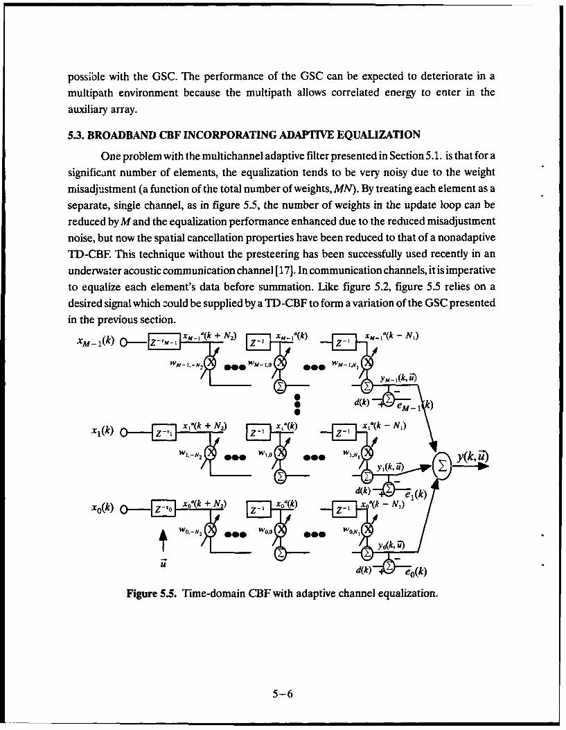
5.3. BROADBAND CBF INCORPORATING ADAPTIVE EQUALIZATION

One problem with the multichannel adaptive filter presented in Section 5.1. is that for a

significant number of elements, the equalization tends to be very noisy due to the weight

misadjustment (a function of the total number of weights, MN). By treating each element as a

separate, single channel, as in figure 5.5, the number of weights in the update loop can be

reduced by M and the equalization performance enhanced due to the reduced misadjustment

noise, but now the spatial cancellation properties have been reduced to that of a nonadaptive

TD-CBE This technique without the presteering has been successfully used recently in an

underwater acoustic communication channel [17]. In communication channels, it is imperative

to equalize each element's data before summation. Like figure 5.2, figure 5.5 relies on a

desired signal which could be supplied by a TD-CBF to form a variation of the GSC presented

in the previous section.X,_ la(k + N2)2 x _ ak)x _lk - NI)

xm - 1k - Z r-I A 1 _,( k)__ _.1 x , _,a(k._"-\

",-'•WM 1o ,.0• ooo 1A-,• ~,

WM -1, N 2 L *** 00 y _# _u

aok) •o(k + N2) Xk) X-(k - N,)

u d(k) e(k)

56

x1(kX,)a Z~ 1 (+N 2) Y a0 k) x '(k-)

WIN2 000 W 000k ~t ~ ~y 0(k,-u

Wd(k) e0(k)

Figrek.5 Z T im-omi C kit +dptv chane equaliz)ationN.

5i-6

6. SIMULATIONS

Two simulations were conducted to compare the performance of the prtsented beam-

forming algorithms. The first simulation considers the case of multiple independent narrow-

band sources while the second simulation considers a single broadband source in a single

multipath environment. Both simulations consider large SNRs only.

6.1. THREE NARROWBAND SOURCES WITH LARGE SNRS

The first simulation compares the TD-CBF, GSC, Bartlett, and MVDR beamformers

for the case of three separate narrowband sources incident on a 10-element linear vertical

array with large SNRs. The MATLAB generation file listed in figure 6.1 shows the details of the

simulation as well as the details of the beamforming and plot generation. The power in the

three narrowband signals differs by 6 dB and all sources are incident at different angk:s, as

described in table 6.1. The array is "cut" for a 25-Hz signal (i.e., the frequency at which the

distance between elements is half the incident signal's wavelength). Appendix A describes the

MATLAB files and their relationships to those generated in [6]. The additive gaussian noise

has a variance of 0.0001. (The adaptive techniques presented here will actually work better

with more random noise because the noise helps to condition the data covariance matrix.)

Table 6.1. Source parameters for first simulation.

Source Azimuth Elevation Frequency AmplitudL. Phase(deg) (deg) (Hz) (deg)

1 90 0.0 25.0 1 02 90 -14.0 45.0 2 45

3 90 30.0 15.0 4 90

Figure 6.2 summarizes the two time-domain beamforming algorithms, TD-CBF andGSC, while figure 6.3 summarizes the two frequency-domain beamforming algorithms,Bartlett and MVDR. Figure 6.2 shows the effects of the anti-(spatial)aliasing filter with theTD-CBE Recall that any incident energy at a frequency greater than that which satisfies the

half-wavelength spacing of the array, here 25 Hz, shows up as a directional ambiguity due to theexistence of grating lobes. When not completely filtered out, the 45-Hz/-14-degree signalcreates havoc in the output beampattern. The antialiasing filter used here is a 29-tap band-passfilter (5-40 Hz) with linear phase. The apparent weak signal incident at roughly +60 degrees

is from the 45-Hz/- 14-degree signal leaking through a grating lobe. The output can beimproved by using a better antialiasing filter. Figure 6.4 plots the power spectral density (PSD)for the TD-CBF and GSC output when they are pointed in the three directions of the incidentsignals. The figure clearly shows that, as expected, the GSC is better able to spatially filter outthe signals not in the steering direction.

6-1

Figures 6.5-6.8 plot the beamforming characteristics for the MVDR and Bartlett

frequency-domain beamforming algorithms. A grating lobe is clearly defined by the 45-Hz/

- 14-degree signal in figure 6.5. The 15-Hz/+30-degree signal creates the sine inverse function

in figure 6.5 described by Eq. (2.5). It is due to spectral leakage (even though a 1024-point FFTwith 50% overlap is used) from the 15-Hz/+30-degree signal, since the background noise is

negligible. Essentially, MVDR is magnifying this minimal energy. When the same simulationwas rerun with a noise variance of 0.01, MVDR displayed spectral peaks, without the sine

inverse effects, as desired.

MVDR seems to work particularly well only at the ideal operating frequency of the

array. For instance, even though the 15-Hz/+30-degree signal has the most power of all

incident sources, the MVDR algorithm does not display the +30 degree direction with the

most output power in figure 6.6. On the other hand, the Bartlett algorithm gives a truer output

value in figure 6.8.

Figure 6.3 plots the sum of frequencies from 5-45 Hz for both frequency-domainbeamformers for comparison with the time-domain beamformer outputs plotted in figure 6.2.

Note the similarities between the TD-CBF and the FD-CBF outputs. When the frequency-

domain beamformers were summed over 5-25 Hz, the 15-Hz/+30-degree and 25-Hz/

0-degree signals are displayed cleanly without the grating lobe interference centered at +60

degree and without the - 14 degree peak.

6-2

" MBi ULVA"% Lniar array of 10 elements spaced 30 meters apart assumed to be% arranged along the z-axis (vertical) with mulztple incident narrowband% sources% Source Azimuth Exmg Eleation A T•h% 1. 90 25 0 1.0 0% 2. 90 45 -14 2.0 45% 3. 90 15 30 4.0 90

% initialize parameters

fs - 1000; % Sample increment (1/1000Hz) (sec)dt = l/(fs);T = 4096; % Number of samplesC s 1500; % Speed of sound (m/sec)M = 10; % Number of elements% Array of element positions along z axis (meters)P = (30) * [ zeros(1,M);zeros(l,M);0:(M-l)];

% generate narrowband complex signals

fLsig = [2545 15]; % Signal's frequency (Hz)amp sig = [ 1.0 2.0 4.0]; % Signal's Amplitudephasesig = 10.0 45.0 90.0]; % Signal's Phase (degrees)az_.;ig = 90 90 901; % Signals Azimuth angle (degrees)el sig = [ 0 -14101; % Signals Elevation angle (degrees)v s 0.0 *ones0lM); % Noise vector% Generate complex element array datadgr = (pi/180); % conversion from degrees to radiansL = length(f sig); % number of signalsX-zeros(MkT);for I:I:L--1

u = [ cos(az..sig(l)'dgr)lcos(el sig(l)*dgr),...

%sm(el]sig(l)°dgr)j;% no noise

X = X+nbsig.en(.sig(l),P,u,ampsigQ),pbasesig(1).dtT.c~v0);endu = cos(az sig(L)'dgr)'cos(el..sig(L)°dgr).

sin(az sig(L) dgr)*cos(e] sig(L)dgr).sin(el.sig(L)*dgr)];

% including noiseX = X+nb siggen(fsig(L),P~u,ampsig(L),phase sig(L),dtTcv);

% Beamifonning

% search directionsaz-q9O];

%*. ............................................ ........% fTeq-domain beamforming% ...........................................................

% beamforming frequencies must be exactly equal to% temporal FFT diorete frequenciesF=[l:59]°fs/1024;

Py=zeros(leng1h(el),length(F));for i: I :lengt(F)

R = sfecsd( X . F(i). P, c. dl, 'OverlapFFr: 1024');PyB(:,i)=bfclass( X. R, F(i), az, el, P, dt, c);PyM(:,i).-vdro(.X R, F(i), az, el, P, dr, c);

end%mesh(flipud(db(Py)'))%conoufiIpud(db(Py)'))%plot(el=db([Py(:.26),Py(:,15),Py(:.46)])) %25.3.14.6,44.9 Hz%poio(F, db()Py(77,:);Py(91,:);Py(121,:)])') %-14de0•deg-30deg%plot(el~db(Lsum(PyB(:.5:46'))aum(PyM(:,5:46'))]) ) % sum over 5-45Hz

........................ ..............................% time-domain beamformnmg% ...........................................................

N = 10;mu - 0.0005; % normalized Ims parameter"% Unear Phase BPF characteristics required for TD Beamforming"% (note 1: with a 20 tap FIR filter, the 0-5Hz is really not attenuated)"% (note 2: group delay 1-10 iterations)a bpf- [11;blbpf - fir I(29.[56fa/2) 40/(fs/2)); % fbegm = 5 Hz - fatop =40 Hz(r m=l:M

X(m.:)=filter(bbpf.a bpfX(m.:));endPy-zero-*length(el),I);B-toeplitz(( I zeros(1,M-3)].,[ -2 I zeros(l.M-3)));for i-1:30:180% conventional time-domain beamforming[P)yCi:i+29),yJ - td cbf(Xjaz.el(i:i+29),Pdtc);% Generalized Sidefobe Canceller[PyG(i:i+29),y] - pc(Xoazel(i:i+29).Pdtc.N,mu.B);

end

Figure 6.1. MATLAB generation file for first simulation.

6-3

0I' v

TD-CBF WITHOUT AA FILTER ,

TD-CBF WITH AA FILTER-10'

-15- '

-.-20S I IS,t%

I i I I I

020

I iIS

-25-*~

-30 -: GSC WITH AA FILTER

-35*" - ,

N= 10-40 '

-100 -80 -60 -40 -20 0 20 40 60 80 100

ELEVATION (deg)

Figure 6.2. TD-CBF and GSC beamforming for three narrowband sources.

0 .

-10-

-20"BARTLETT

" -30-

Ii

0 40-

II II

-5 0 -:, , ,"II !I t SI 1

60 ---- ---------------- ,----" , ,SI I DI# Io ,• ,l

S *

MVDR

-70 , 6

-100 -80 -60 -40 -20 0 20 40 60 80 100

ELEVATION (deg)

Figure 6.3. Bartlett and MVDR beamforming summed from 5 to 45 Hz for threenarrowband sources.

6-4

+30 deg N.

.. -14 degS... .. / 0 deg

-20 I* I

-40-

60•

0 -60

S-60 -, ,

1 ..-80 -

-100

TD -CBF

-1200 10 20 30 40 50 60 70 80

FREQUENCY (Hz)

0+30 deg

IS

-20 - 0 deg

-14 deg

-40

S-60 "

a*s

-80- ,

-100-

GSC

-120 1 a '0 10 20 30 40 50 60 70 80

FREQUENCY (Hz)

Figure 6.4. TD-CBF and GSC PSDs along -14-, 0-, and +30-degree steering directionsfor three narrowband sources.

6-5

FRQEC6Hz0~EEATO dg

09

FREQUENCYLEVTO (deg) EEVTON(dg

40-6

STEERING DIRECTION FIXED:-10 5

* S

-20

-30 • 0 deg

"o -40 -14 deg

+30 deg~-50-

0

-60.

-70 :.,-- .. "

-80 ".... , , . ..- "

-90 -II

0 10 20 30 40 50 60

FREQUENCY (Hz)

-10 FREQUENCY FIXED

25.3 Hz-20

-30 44.9 Hz

.-- 40- ,--'• -4014.6 H-z

S-50-

-60u

...... ....- .. ....-80 - ..- ...

-901-100 -80 -60 -40 -20 0 20 40 60 80 100

ELEVATION (deg)

Figure 6.6. MVDR beamformer output for three narrowband sources along fixed steeringdirections (top) and along fixed processing frequencies (bottom).

6-7

FRQEC6H)ELVTO0dg-900

-90

00

50-

Ux~ocoo~ cz

10-8

STEERING DIRECTION FIXED

-10 .. +30 deg

-1e0 deg-20- 14 deg

-30 : ..

-50 -'-

3 m I C.

-60 .."/:" I

-70 %

-80 - .

-90-

-1000 10 20 30 40 50 60

FREQUENCY (Hz)

0 -

FREQUENCY FIXED , ",, . 14.6 Hz

-10 44.9 Hz/ * i : "' - -.. . .

-20 -. -- ,,-'

-30 ..

~-40-aI

S-500

-60

-7025.3 3Hz

-80-

-90 ,

-100 -80 -60 -40 -20 0 20 40 60 80 100

ELEVATION (deg)

Figure 6.8. Bartlett beamformer output for three narrowband sources along fixed steeringdirections (top) and along fixed processing frequencies (bottom).

6-9

6.2. SINGLE BROADBAND SOURCE WITH SINGLE MULTIPATH

The second simulation compares the TD-CBF, GSC, Bartlett, and MVDR beam-

formers and the multichannel adaptive filters for the case of a single broadband source

incident at 0 degrees and its single multipath incident at -14 degrees on a 5-element linear

array. The MATLAB generation file listed in figure 6.9 shows the details of the simulation aswell as the details of the beamforming and plot generation. Figure 6.10 shows the PSD of the

broadband signal and the received data at element 1 and element 5. The broadband signal

generated by the MATLAB file "bbsig__gen.m" (see Appendix A) is composed of four

separate components: (1) 15-25 Hz band-pass filtered noise which is amplitude-modulated at

2 Hz, (2) exponentially low-pass filtered noise, (3) a narrowband signal at 18 Hz, and (4) three

odd harmonics of the narrowband signal at 24.17 Hz. The effects of the multipath are clearly

seen as spectral notches (refer to Section 2.4) in the received data's PSDs. The channel is

modeled after the simulation outlined in Section 2.3. The FIR filter coefficients for each

source-to-element channel are defined as

b(1,:)=[ 0.9 zeros(1,31) 0.9 0 0 0 00.000000.00000 0.00 0 0 0 0 0.00];b(2,:)=[ 0.9 zeros(1,31) 0.0 0 0 0 0 0.9 0 0 0 0 0.0 0 0 0 0 0.00 0 0 0 0 0.001;b(3,:)=[ 0.9 zeros(1,31) 0.0 0 00 0 0.0 0 0 0 0 0.9 0 0 0 0 0.00 0 0 0 0 0.00];b(4,:)= [0.9 zeros(1,31) 0.0 0 0 0 0 0.0 0 0 0 0 0.0 0 0 0 0 0.85 0 0 0 0 0.00];b(5,:)=[ 0.9 zeros(1,31) 0.0 0 0 0 0 0.0 0 0 0 0 0.0 0 0 0 0 0.00 0 0 0 0 0.471;

which defines the direct path incident at 0 degrees (interelement delay equals 0) and the multi-

path incident at - 14 degrees (interelement delay equals 5). The total power in the multipath is

roughly 0.8 times that in the direct path.

Figures 6.11 and 6.13 summarize the results of the two time-domain beamformers, and

figures 6.12, 6.14-6.17 summarize the results from the two frequency-domain beamformers.

In figure 6.11, the TD-CBF displays both direct and multipath incident directions. However,

the GSC displays no multipath at - 14 degrees because the direct path is adaptively filtered by

the auxiliary arrays and subtracted from the main array's multipath output. As can be seen in

figure 6.13, neither beamformer eliminates the spectral notch created by the multipath.

In figures 6.14 and 6.15, MVDR is seen to effectively lock in on the 24.17-Hz narrow-band signal, giving excellent directional data at 24 Hz for both the direct and multipath signals.

However, the multipath signal is displayed at a power level significantly lower than the actual

incident power level, presumably because of the strong correlation with the direct path source.

The Bartlett beamformer, plotted in figures 6.16 and 6.17, has significant difficulty in any

directionality, presumably because of the wide beamwidths of the 5-element array. However,

it is readily apparent from the PSDs along the 0-degree and - 14-degree direction in figure

6.17, that the two signals are related. This was not the case for the MVDR algorithm in figure

6.15.

6-10

Figure 6.12 plots the su; .1e frequency-domain beamformer outputs from 5-45 Hz

for comparison with the time-domain beamformer outputs in figure 6.11. The MVDR beam-

former displays peaks at the correct directions corresponding to the incident direct and multi-

path signals, but the relative power between the signals is significantly different than the actual

0.8. It is interesting how much better the TD-CBF (using the same antialiasing filter as before)

did with respect to the Bartlett beamformer. One might have expected similar results between

the two, as was the case for narrowband signals in the previous simulation. This might be due to

energy at frequencies greater than 45 Hz or to differences in the spatial-temporal correlation

matrix and the spatial-spectral correlation matrix as suggested by [41].

The weights of the multichannel adaptive filter described in Section 5.1 are plotted in

figure 6.18 for presteering angles of 0 degrees and - 14 degrees and N1 =N2 = 75. The weights

show that in both cases, the signal with more power (0-degree incident signal) is interpreted as

the direct path by the filter. Thus, as long as both direct path and multipath lie within the

multichannel adaptive filter's spatial window defined by N (refer to Section 5.1), the output

power contains no directional information. However, the weights could be further processed

to obtain directional information. Figure 6.19 shows that the PSD of the multichannel adaptive

filter output has been equalized since no spatial nulls exist. Figures 6.20 and 6.21 plot the

weights of the multiple single-channel adaptive filters discussed in Section 5.3 for N1 =N2 = 75

and N1 =150, N2 =0. The weights are seen to take on values described by Eq. 2.20.

6-11

"% MPATH ULVA"~ This scr~it file generates the Uniform Linear Verical Array"% element time-.series inputs for a multipatb environment. The multipath

" is generated by propagating a signal (broad or narrow band) through"% separate channels (modeled as as ARMA linear filter) between each sensor"% and a single source.

% written by: Rich North 1-1-92

% initiaize parameters

T - 8192; % Number of santples(2^ 13)fs - 1000; % Sample frequencydi - lI~s); % Sample increment (sec)c - 1450; % Speed oftsound (ot/ac)M -S; % Number of sensors in arrayX-zeros(M.T); % array element time-series datafOs24.17, % primary CW wave (d - lambda/2)% Array of sf sigpen positions along e axis (meters)P -(30) * [zeros(l.M);zeros(l.M);0:(M-1)];

% generaie signal

% (real) broad band signalssbbsig~gen(T,25.0.l 5.040.18,fs);

% propagate signal through ARMA channel

rand('normal');avar - 0.01;anoise - sqrtgnvar);a - zeros(l.T);%source-gensorfl-M channela - I I];Lfir-S3;b-zeros(MjLfir);b(l.:)=( O:9 -rs( ')090 00000000-00000000.000000];b(2,:)= 0.9 :2o(213 1) 0:0000000 00.9 00 00 0,0 0 00000.0 000 0 0;b(3,:)-I 0.9 zeros(1,31)0.0 0 00 00.0 000 00.90 0 0 0 00000001;b(4.:)=[ 0.9 zeros(0.1) 0.00 0 000.0 0 00 00.0 0 0 0 0 08500000).b(5,:)=[ 0.9 zeroa(1.31) 0.0 0 0 000.0 00 00 0,0 00 000.0 00 0 00.47];for m-l:M

u-filier(b(m,:).a.s)+anouerfand(u);

end

% Beamforming

% search directionsAZ-f 90];

%............................000000*.......% freq-dornain beam) orming

*.......................... ...........% beamforming frequencies muat be exactly equal to% temporal FF1'discete frequencies%F.11:591'fs/1024;*Py-zeos0ength(el).legth(P));%for i=1Liength(F)% R - sfecsd( X . Fft) P , c. dt. 'OverlapFVT: 1024');% Py(:.i).bfclass X. R, F(i). atz. el, P, dl., c);% Py(:.i).mvdr( X, R. F(i). az, eL, P, dt, c);%end%ploigel~db([Py(:,2),Py(.,10),Py(.,19)])) %24.4,9.8,18.3 H4z

*plor(P~dbq(Py(77.:);Py(91.:)J)') % -)4degOdeg*plot(eLdb(sum(PyB(l :180.5:45)*).eL~db(sum(PyM(l :180.5:45)')))

% time-domain baforming

% LMS filter parametersN - 150;mu - 0.05; % alms parameer% Linear Phase BPF elisracteriatics required for .9 Beamforinga bpf= [11;

b-bpf- firl(294j5i/fst)40I(fu/2)]); % fbegin -S5Hz -ftop -40 Hzfor m-1:M

X(m.:)w.lilter(bbpf.&bpfX~m,:));end

*Py-wosoength(el)4I);%B-toeplitz([ I zeros(l.M-3))MI -2 1 zeros(lM-3)]);%for i-1:30:180% conveniional time-domain beamforning%IPy(i:i.29).yJ = t cbf~Xazecl(i:i+29),P~dc);% conventional time-domai beamforming w/ single channel equalization*Jpy(i:i429.yJ - deql(X~aueli:i+29,P~dt~cN~mu~s)% Generalized S-idelobe Canceller%(Py(iHi29).yj - p(X~az~eli:i+29).0d,cftNNmu.B);% Multichainel Adaptive Filter%jPy(iHi29).yI - mch~aft-elA(i:i429)P.dt~cNmu~A)

%end

"*[PY(91).y] . gcXael(91.P~dt"cN,muB)," Pxz2 - scrum~y,1024.75);

%p ot(F.db(I Px(l:59,l)';Pxx2(l:59.l)'j)) % -1 4deg.Od

Figure 6.9. MATLAB generation file for second simulation.

6-12

103

BB SOURCE

102

101 * ~ 1

10.0

10.?0 50 100 150 200 250

FREQUENCY (Hz)103

X( 1,:

102

101 NJ

cA 100

10.1

10-2-

10-3,0 50 100 150 200 250

FREQUENCY (Hz)

103

102

101

100

10'

10.2 0010205

FREQUENCY (H1z)PSDs +/- 95% CONFIDENCE LEVELS

Figure 6.10. PSD of transmitted broadband source and received datafrom element 1 and 5.

6-13

0

-2-

-3 TD-CBF

S -4-I'

-~)it

It-5-

-6-

,:,,,, :,:,. ,i4 . ,,, , . ..,-7 "" , ,, :

i it' I I it I IIg+#I+S_. -, +,,.. .. GSC

-100 -80 -60 -40 -20 0 20 40 60 80 100

ELEVATION (deg)

Figure 6.11. TD-CBF and GSC beamforming for a single multipath.

0

-2-

-4: , BARTLETI"

-6 ,' - ,,

•" -8S-10

091- -12

-14S SS°

-16 "" • MVDR"

-18 ,-

-201-100 -80 -60 -40 -20 0 20 40 60 80 100

ELEVATION (deg)

Figure 6.12. Bartlett and MVDR beamforming summed from 5 to 45 Hz for a singlemultipath.

6-14

15 *

-20 -14dde

Sl I I # I

- 0 1 2

I

- 5 -I ,

,

-15 0'

-5-•

0-20-

-- 14 deg

-25

-300 10 20 30 40 50 60

FREQUENCY (Hz) ALONG -14 deg AND 0 deg

-5

-10

. -14 deg-25

-30 I

-350 10 20 30 40 50 60

FREQUENCY (Hz) ALONG -14 deg AND 0 deg

Figure 6.13. TD-CBF and GSC PSDs along -14- and 0-degree steering directions for a

single multipath.

6-15

FRQECY(0 EEAI-900

09

00

50 -:7W

~40-

>- 30U

-90 -70 -50 -30 -10 10 30 50 70 90ELEVATION (deg)

Figure 6.14. MVDR beamforming for a single multipath; FF1' size of 1024 points.6-16

0 1 1

STEERING DIRECTION FIXED

-5-

-10-

9.8 Hz-15

0

-20

-25-

24.4 Hz

-301-100 -80 -60 -40 -20 0 20 40 60 80 100

ELEVATION (deg) AT 9.8, 24.4, 18.5 Hz

0I,

.¶ :~FREQUENCY FIXED-2-* * ~ *

0 'deg

-4 : ,

is gIt• *I_. -6. " " ;0 ' , I ; II

Si#-8 ': •I•: : - ,

0-10-

-12-

-14 1--4deg

-160 10 20 30 40 50 60

FREQUENCY (Hz) ALONG - 14 deg AND 0 deg

Figure 6.15. MVDR beamformer output for a single multipath along fixed steeringdirections (top) and along fixed processing frequencies (bottom).

6-17

60

90

FREQUENCY (Hz) 090ELEVATION (deg)

0 -90

50

20

-90 -70 -50 -30 -10 10 30 50 70 90

ELEVATION (deg)

Figure 6.16. Bartlett beamforming for a single multipath; FFT size of 1024 points.6-18

01STEERING DIRECTION FIXED

-5-

"10 18.5 Hz

- -15

. . . . . .. . . . ... ... ..

-25- 9.8 Hz

-30 /24.4 Hz

-35

-40-100 -80 -60 -40 -20 0 20 40 60 80 100

ELEVATION (deg) AT 9.8, 24.4, 18.5 Hz

0FREQUENCY FIXED

-5--50 deg

-10-

2 -20--o1 -. deg

-25

-30

-35 10 10 20 30 40 50 60

FREOUENCY (Hz) ALONG - 14 deg AND 0 deg

Figure 6.17. Bartlett beamformer output for a single multipath along fixed steeringdirections (top) and along fixed processing frequencies (bottom).

6-19

0.16PRESTEERING = 0 deg

0.142 1

0.12 34

0.1 I

S

0.08-

0.06 5'.

0.04-

0.02-

0-

-0.02

-0.04,0 20 40 60 80 100 120 140 160

WEIGHT NUMBER

0.14

PRESTEERING =-14deg 1 2 3 4 5

0.12

0.1

0.08-

0.06

0.04-

0.02

0

-0.02

-0.040 20 40 60 80 100 120 140 160

WEIGHT NUMBER

Figure 6.18. Multichannel adaptive filter weights for a single multipath: presteering at 0(top) and -14 (bottom) degrees [N1 =N2 = 75].

6-20

0

-2- 0-60 Hz

-4-

-6-

-8-

-10-

-12-

-14-

-1610 10 20 30 40 50 60

FREQUENCY (1hz)

PSD (dB)

103

0-250 Hz

102

10

II S~d;r

10-1

PSDs +/-95% CONFIDENCE LEVELS10-2

0 50 100 150 200 250

FREQUENCY (Hz)

Figure 6.19. PSD of multichannel adaptive filter output for a single inultipath:presteening of 0 degrees [N1 =N2 = 75].

6-21

0.8PRESTEERING = 0 deg

0.6

0.4 21

43

0.2-5

-0.2-

-0.40 20 40 60 80 100 120 140 160

WEIGHT NUMBER

0.8

PRESTEERING = -14 deg

0.65

41

0.4 23

Z.

0.2-

0

-0.2

-0.40 20 40 60 80 100 120 140 160

WEIGHT NUMBER

Figure 6.20. Weights of the multiple single-channel adaptive filter for a single multipath:presteering of 0 (top) and - 14 (bottom) degrees [N1 =N2 = 75].

6-22

PRESTEERING -0 deg

0.8

0.6

0.4

0.2- 2 3 4

-0.2-

*I|

-0.4- ''''0 20 40 60 80 100 120 140 160

WEIGHT NUMBER

Figure 6.21. Weights of the multiple single-channel adaptive filter for a single multipath:presteering of 0 degrees [NI = 150, N2 =0].

6-23

7. CONCLUSION

This report has introduced and discussed the spatial -temporal processing capabilities

of several adaptive and nonadaptive beamformers. Table 7.1 summarizes the results. Only the

multichannel adaptive filter was found to be able to adaptively cancel uncorrelated interferers

as well as to equalize the direct-path source with its correlated multipaths, true spatial-

temporal processing. It was shown, however, that some a priori information about the source

signal is needed for equalization and that the multichannel adaptive filter did not provide

directionality information without a further processing of the weight values. The frequency-

domain MVDR and the time-domain GSC beamformers were both shown to perform only

spatial processing (adaptive interference cancellation) and no temporal processing. Further-

more, the performance of both algorithms degrades with the correlation of the interferers,

greatly reducing the usefulness of these algorithms in a multipath environment. In short,

further research is required to generate a true spatial-temporal beamformer. One possibility

might be to incorporate blind equalization (equalization without a desired signal; see

NO TAG) into the multichannel adaptive filter and develop a method of extracting directional

information from the adapted weight matrix.

Table 7.1. Capabilities of beamforming algorithms.

Algorithm Capabilities

Adaptive Interference I Source-Element I Performance AffectedCancellation EqualizationI by Source Correlation

Frequency DomainBartlett No No NoMVDR Yes No Yes

Time Domain

TD-CBF No No NoMulti-Ch AF Yes Yes NoGSC Yes No YesMultiple No Yes NoSingle-Ch AF

7-1

8. REFERENCES

General DSP

[1] D.J. DeFatta, J.G. Lucas and WS. Hodgkiss, Digital Signal Processing.:A System DesignApproach, John Wiley & Sons, NY, 1988.

[2] E J. Harris, "On the Use of Windows for Harmonic Analysis with the Discrete FourierTransform," Proc. IEEE, vol. 66, pp. 51-83, Jan. 1978.

[3] S.M. Kay and S.L. Marple, "Spectrum Analysis-A Modem Prospective," Proc. IEEE,vol. 69, no. 11, pp. 1380-1419, Nov. 1981.

[4] W, Press, B. Flannery, S. Teukolsky, and W Vetterling, Numerical Recipes in C,Cambridge University Press, 1988.

General Adaptive Beamforming

[5] J.C. Allen, 'Array Gain in Anisotropic Noise," Working Papers, Sept. 1992.

[6] J.C. Allen, "Direction Finding Database and Techniques (DFDT)," NOSC TN 1657,May 1991.

[7] W.S. Burdic, Underwater Acoustic System Analysis, Prentice-Hall, 1984.

[8] R.T Compton, Jr., Adaptive Antennas: Concepts and Performance, Prentice-Hall,1988.

[9] D.H. Johnson and D.E. Dudgeon, Fundamentals of Array Signal Processing, to bepublished, Prentice Hall, 1993.

[10] R. Schreiber, "Implementation of Adaptive Array Algorithms," IEEE Trans. onAcoustic, Speech and Signal Processing, vol. ASSP-34, no. 5, pp. 1038-1045, Oct.1986.

[11] R.J. Urick, Principles of Underwater Sound, McGraw-Hill, New York, 1983.

Adaptive Equalization and Deconvolution

[12] R.A. Axford NRaD Code 844, Notes and Conversations, 1992.

[13] J.V. Candy, R.W. Ziolkowski, and D.K. Lewis, "Transient Wave Estimation: AMultichannel Deconvolution application," J. Acoust. Soc. Am., vol. 88, no.5, pp.2235-2247, 1990.

[14] S. Haykin, Adaptive Filter Theory, 2nd Edition, Prentice Hall, 1991.

[15] David Middleton, "Channel Modeling and Threshold Signal Processing in Under-water Acoustics: An Analytical Overview," IEEE Journal of Oceanic Engineering, vol.12, no.1, pp. 4-28, 1987.

[16] J. Proakis, Digital Communications, McGraw-Hill, New York, Ch. 6 & 7, 1989.

[17] M. Stojanovic, J. Catipovic, and J.G. Proakis, "An Algorithm for MultichannelCoherent Digital Communications Over Long Range Underwater AcousticTelemetry Channels," preprint from J. Proakis, Northeastern Univ., July, 1991.

8-1

Curved Wavefronts Due to Nonuniform Sound Speed Profiles

[181 E. Webster NRAD Code 782, Notes and Conversations, 1992.

Time-Domain Beamforming

[191 M.G. Bellanger and P.A. Regalia, "The FLS-QR Algorithm For Adaptive Filtering:The Case of Multichannel Signals," Signal Processing, vol. 22, pp. 115-126, 1991.

[20] K.M. Buckley, "Spatial/Spectral Filtering with Linearly Constrained MinimumVariance Beamformers," IEEE Trans. on SP, vol. 40, no. 8, pp. 2112-2116, Aug. 1991.

[21] O.L. Frost, "An Algorithm for Linearly Constrained Adaptive Array Processing,"Proc. of the IEEE, vol. 60, pp. 926-935, Aug. 1972.

[22] S. Godard, "Channel Equalization Using Kalman Filter for Fast Data Transmission,"IBMJ. Res. Develop., pp. 267-273, May 1974.

[23] L.J. Griffiths, "Signal Extraction Using Real-Time Adaptation of Linear Multi-channel Filter," PhD Thesis (Tech Report No. 6788-1) Standford University, Feb. 1968.see also L.J. Griffiths, "A Simple Adaptive Algorithm for Real-Time Processing inAntenna Arrays," Proc. of the IEEE, vol. 57, pp. 1696-1704, 1969.

[24] L.J. Griffiths, and C.W Jim, 'An Alternative Approach to Linearly ConstrainedAdaptive Beamforming," IEEE Trans. onAntennas and Propagation, vol. 30, no. 1, pp.27-34, Jan. 1982.

[251 E Lung and J.G. Proakis, 'A Generalized Multichannel Least Squares LatticeAlgorithm Based on Sequential Processing Stages," IEEE Trans. on Acoustic, Speechand Signal Processing, vol. 32, no. 2, pp. 381-389, April 1984.

[26] R.G. Pridham and R.A. Mucci, "Digital Interpolation Beamforming for Lowpass andBandpass Signals," Proc. of the IEEE, vol. 67, no. 6, pp. 904-919, June 1979.

[27] J. Ward and R.T. Compton, "Sidelobel Level Performance of Adaptive SidelobeCanceller Arrays with Element Reuse," IEEE Trans. on Antennas and Propagation,vol. 38, no. 10, pp. 1684-1693, Oct. 1990.

[28] B. Widrow, RE. Mantey, L.J. Griffiths, and B.B. Goode, '"Adaptive Antenna Systems,"Proc. of the IEEE, vol. 55, pp. 2143-2159, Dec. 1967.

[29] H. Ye and R.D. DeGroat, 'A Generalized Sidelobe Canceller with Soft Constraints,"IEEE Trans. on ASSP, vol. 35, no. 3, pp. 249-266, March 1987.

Frequency- Domain Beamforming

[30] BBN Systems and Technologies, "Issues in Adaptive Beamforming," NOSC Tech.Doc. 2105, May 1991.

[31] S.I. Chou, 'A First Look at Narrowband Array Processing and Implementation for anExtra Large Multi-Dimensional Array," NOSC Tech. Note 1654, Mar. 1991.

[32] H. Cox, "Resolving Power and Sensitivity to Mismatch of Optimum ArrayProcessors," Journal ofAcoustical Soc. ofAmerica, vol. 54, no. 3, pp. 771-785, 1973.

8-2

[33] H. Cox, R.M. Zesking, and M.M. Owen, "Robust Adaptive Beamforming," IEEETrans. on Acoustics, Speech and Signal Processing, vol. ASSP-35, no. 10, pp.1365-1376, 1987.

[34] M.D. Green (BBN), "STRAP: Baseline Definition and Performance Analysis,"NOSC Tech. Doc. 888, April 1986.

[35] S.K. Lapic, J.C. Lockwood, and D.F Gingras, "The Effects of the ConventionalBeampattern on Adaptive Beamformer Performance," NOSC Tech. Doc. 1307, Dec.1988.

[36] G.L. Mohnkern, "Effects of Errors and Limitations on Interference Suppression:Preliminary Report for the High Gain Initiative," NOSC Tech. Doc. 1478, Feb. 1989.

[37] M. Reuter, "Characterizing and Improving the Performance of the MVDRProcessor," NOSC Tech. Doc. 1983, Nov. 1990.

[38] D.WJ. Stein, "Beamforming in the Presence of Moving Sources," NOSC Tech. Note1655, March 1991.

[39] C.V. Tran, "Effects of Steering Vector Errors on MVDR and Signal SubspaceBeamforming," NOSC Tech. Note 1649, Mar. 1991.

[40] J. Tran, "Approaches to the Processing of Data from Large Aperture Vertical LineArrays," PhD thesis, University of California, San Diego, (also SIO reference 90-21),1990.

Effects of Correlated Sources[41] J. Krolik, and D. Swingler, "Multiple Broad-Band Source Location Using Steered

Covariance Matrices," IEEE Trans. on Acoustic, Speech and Signal Processing, vol. 37,no. 10, pp. 1481-1494, Oct. 1989.

[42] B. Madan and S. Parker, "On Adaptive Beamforming in Correlated Noise," CircuitsSystems Signal Process, vol. 7, no. 3, pp. 327-343, 1988.

[43] A. Paulraj and T. Kailath, "On Beamforming in Presence of Multipath," Proc. ofICASSP-85, pp. 564-567, 1985.

[44] V. Reddy, A. Paulraj, and T Kailath, "Performance Analysis of the OptimumBeamformer in the Presence of Correlated Sources and Its Behavior Under SpatialSmoothing," IEEE Trans. on Acoustic, Speech and Signal Processing, vol. 35, no. 7, pp.927-936, July 1987.

[45] T-J. Shan, M. Wax, and T. Kailath, "On Spatial Smoothing for Direction -of-ArrivalEstimation of Coherent Signals," IEEE Trans. on Acoustic, Speech and SignalProcessing, vol. 33, no. 4, pp. 806-811, Aug. 1985.

[46] K. Takao, N. Kikuma, and T. Yano, "Toeplitzization of Correlation Matrix inMultipath Environment," Proc. of ICASSP-86, pp. 1873-1876, 1986.

[47] B. Widrow, K. Duvall, R. Gooch, and W Newman, "Signal Cancellation Phenomenain Adaptive Antennas: Causes and Cures," IEEE Trans. on Antennas and Propagation,vol. 30, no. 3, pp. 469-478, May 1982.

8-3

Appendix AMATLAB ROUTINES

This Appendix describes the MATLAB routines used in this text to compareperformance between various beamforming algorithms. MATLAB routines are patternedafter those written by Jeff Allen [6]. The input-output vectors and notation have beenmatched to those used by Jeff Allen [6]. Figure A.1 highlights the interaction between theMATLAB programs. Element input data are typically stored in the time-domain arrayX, withT time-domain inputs from each element of an M-element array as

T time samples

xo(n) x0(n- 1) ... xo(n- T+ 1) AI x'(n) xi(n - 1) ... xi(n - T + 1)) j

X x2(n) X 2( x2(n - T + 1)1 M elements (A. 1)

[xM-(n) xm_,(n - 1) ... xM_,(n - T + 1)]

The M-element array (X,Y,Z) locations are stored in the array P:

lM lements

xO X1 X2 ... XM- 1 1 (A.2)P= YO Y1 Y2 ...YM-,

Zo ZI Z2 ... ZM-1 I

The steering matrix can be formed as time delays for multiple azimuthal angles, 0, and multipleelevation angles, 4p:

44 n az*n el

_ [ri6o,0) T016,00) ... r]0,1 r)0,1 .. r)(00,02) rI10.002) *.A= 2(00_00) T2(01,00) "2(00,0 1) •20(1,01) .2(.00.0 2) T2(0 1,0 2) elements (A.3)

A - ?3(Oooo) r 3 (0 1 ,0 0 ) *r3(00"01) r 3 (0 1 ,0,) .r 3 (0• 0, 2 ) r 3 (0 1 ,0 2) . Mv

or phase delays

naz*nel

A = exp j 2 ;r f ?2(0oo) r(0,,Oo) ... r2(00,0) T2(0,01) ... T2(00,02) r2(01,02 . (A.4)r3(00,00) T[3(01,00) .. 3(00101) T3(01,01) ... 3(0•0,0) T301-,02.)..t

The beamformer output power is stored in the array Py (Y is the notation used in [6]) formultiple azimuthal angles, 0, and multiple elevation angles, 40,

- y(,,01) y(Y(01101) X1,,02) y(A,03) . (A.5)

A-1

VECTFORMGDIPASPECTRALIO (bfclas.m, UPU

REALMEIU DAAALINTAMOMN

2. StaL nc-ln~

3. Kavg~eh gcmm

Fb-igure A.1. BlockAT darmobefoinsgnal rocessngoptdwihMTA

1. RI stem (oiid sihl rom [6])r

SIMULTIO. bbsiggen1.~ ~ ~~~3 XGSMDT ATRIgBOADAN

1. MDA- (xafi4.c (tdcbff~m2. ~ ~ 5 mtrapnlmsims3. ~ ~ 6 gsch g~m4. ~ ~ 7 Sarahaf f~

8.in variosaoucepoaipudtaThe fllowng NAT9. programs~ (modiused sligtesvly fro [6])eot nrelstdi

10.i mntiret (mdiie slightl from[6]11. steer.m (modified slightly from [6])

functionA ~~2 bbera~e,~~o~tig % singgam: (:knI uk)c

% TER ceaesanarayo seengveto fr hegie az~imuh nd kweeuk stektblo etro eghI eemnda olw

55 ~ ~ ~ ~ ~ 8 P-3sararayesnarpatinsmc ~ ~ ~ ~ ~ 9 M-asr smoeede ofghl figna [6pgto kcs~zql)o~lp1))

9k trng Tas otpt pas dla (eful 1. notr~ deodined) slghl frome~p [6))

functio e oupu s t imer delay~cD (secondg) % un* Tm' (,) Puk

9k OIJFPUT: ltiM den ;oste h nmerm of ser wher u111 isen thefr C-. okvco o eghMdtrmnda on%~~~~~~~~~~ nazrs fo thnehaz give aDirecuio aidnnatdaead ehiue

%k form tio anlsa ivni 1 functionr It a ster ze ~ tig

9k stZn - v haeto o df aziutanl es A(: e) % s(i2pilPuk

% ~ ~ ~ ~ ~ Fgr el2 MAL- etro lvtosage dg hnodsrigte listLBcnetofr igs.s trin t .w geotd

P -UM rra oftheM snso poitAns2

n az -n %-------a----ne egt)i) % generate sinusoids

u az: 180ssziI ); sin(az~pi/180); ones(l n 10 foa 1:2:5Uc D(]P/8) i(elpýI/T80) I - s + 0.9 -icoos(2'pi~i10f~tt); % stnusoid

ucl cosel /180: ca~eli/10); lflend:

"% for the k-th elevation angle, produce the look Vector containing all phase =p4.6 an ponstantI phase .soi"% the azimuth angless s+ .csrflf +Pae; snoiA - zeros(3, n az~nel);for k1l:n el_ _ iig~A(;. (0 ~iz(k-i)+1I):(n az'k)) =u~az (u el(:.k) ones(l,n~az)); X lg~

end

% calculate delay XAGNif (nargin < 6) *This matlab mex function delays and weights the tume series

A - exp( i"2*pi~fDP'*A/c) data from multiple sensors and stores the aligned data forelse *more processing.if (strcmp( string. 'Phase' ))

A;= exp( i*2*pifO*P'A/c) USAGE FROM MATLA13:elseIf strcmp) string, 'Time') Xa-Xalign(XYru)

A = P'A/c;else *TO COMPILE:

error(' ... string set incorrectly (Phase or Time) .')noatlabibin/cmex Xalign.cend

end *INPUTS:

*X - MaT matrix where each row consists of the time sertes*data front a sins e element

bb-si~ gen* M - number of elementsT-nmeofdata aampels

TU-MImatrix of delaysfunction s-bb sig en(T~nvarIsvar2Jf0.flM)

% .. 0. ... r ý ............ .......... OUTPUTS:"% BB SIG GEN: *Xa - MxT matrix of weighted and delayed X elements"% ThR mailab function generates a broad band signal with odd *AGR~M"% harmonics.LORTM

% INPUTS: -X(m~t-tau(msu))

% T - number of data samples (T>2*N) Xa(m~t)% nvarl -variance of the noise, varjnl njl 0 (if X(m~t-tau(mu~t)) not in matrix)% nvar2 - variance of the noise. vartn2 nj"% ff1 - primary sinusoid frequency REharmonic:"% fl - secondary sinusoid frequency R.K North, "Broadband Conventional Beamforming Incorporating"% fs -sampling frequency Aodaptive Eqlualization," NRaD Tech. Note 1992

% OUTPU~s: *witnb:RcadNrh59

% s - lxT vectortoftbroad band data........................ ..............% *include 'emath.h>

% ALGORITHM: #tnclude <sdobh>% *include "cmex~i"

% Amp Modulation%c+a(n) /I inpu rsnns'

%- a Idefine X IN Frhs[01% nI(n)- -- I BPF j-f(tt)- "--+ -- s(n) #defin TAU_ IN pebsjI]

*-= #eIneXlind OUT plbs[OJ% n2(n) - - - LPF 1-(n) - --- +

%W user fcn(nlhs~plhsnrhs~prhs)% int nls~nrhs;

% tinQO/tfs)- -- -- -- -- -- ---- Matrix *pffsfl, prhsl];% sin(3ftf) - -- -- -- -- ---- /*Matlab variables/

% I unsigned ins MNlooksT;% sin(Slflf) - -- -- -- -- ---- double Xe,*X-im,"TAU,*Xalignedre.Xaligned im;

% sin(fI/fs)---- -- -- -- -- - - -I /Iisc local variab~les/% ins cUmnA.adelaydelay-a

% 9-bb sigjenCTnvarI,nvar240Jl~s) r check number of arguments I/% writttn by: Richard North 6/92 i ob 2 c ro(Xlg eurs2ipt.)

i f(n s- I) men error("ai requires I output. ;

% - - -- - - -- ---P set variables and allocate memory */% initialize variables M-TAU-IN->m; r #ofrows equals# ofelements/% - - - - -- -- -- -if(X IN-'m !- M)

t-0:1:T-1; % t-0.1.,23,..T-J- time meiefror("Xali requires X, and tau to have same number of elements.");anotsel - sqrt Iar~ Nlocka - TAU IN- >n; r * ofcoulumns equals # of steer directions *1anoiae2 I- Tnnva,2ý; if (Nooks I- IT rqie nyl,,rand'ormal) T1.= InN~r-r>n; /E of columns equals# of time samplesI

% - - -- - - -- ---X -re -X IN- >pr.% generate amplitude modulated bandpass noise X im: - IIN- >pi;

% - - - - -- -- -- -TAU -TA1JIN- >prn - anoisel~rand(t); % random noisflow - 5/(fs/2); df(X isn NULL) I-real/fhigh 25/(fs(2);

(baIbutter(54flow flush)); % 10th ordered band pan filter Xaligssed OUT - create lnatrix(M.ItREAL),n-fllter(biain); T band peaw filtered noise Xaliged~re - Xahiged -UT- >pr,

C'.03; % C-0.0 - >nomoda - oncs(t) +C~cos(2"pis2Jfst)).*fn; % amp mod (2 Hlz) bpf noise else P* complex '

% - - - - -- -- -- -Xalligsed OUT - create imatxM.T.COMPLEX);* generate exponentially filtered low pan noise Xaligned-re -Xaligned -UT- >pr;

* - - - - -- -- -- -Xaliw d:iy- Xaligned- OUT- >pt;o - anotse2*rand(t); % random noisefI -1:10 V10;in. I en(-OyV)'; %0hdrdopnitTif (Xim - NULL) r real

bflr2(Il.j n); %1t ree o asflea-ll . do dely ad weigbting o ahtm

-Ia+ fllter(b~a.n); %asonl + filtered noise P NOTE atlab sto :resb oun ota X(i~j)- Xji+7bsalNrowsi1jIf we only have vectors, this is transparent/

Figure A.2. Continued. (Contd)

A-3

for (t10; t<T; t+ +) Y - zeros(Nlooks.T);Py - zeros(l,Nlooks);

P across elements "x = zeros(tl );for (me0; m<M; n+ +)

a - t-(int)TAU[ml; 9, Generate steering time delays for all directtons of lookif((a >= 0) && (a < T)) % ..... . = . ...... .... ...... .........

Xalignedrem+M~t] = Xere[m+M*al; A = steer( az. el, P, c, I, ,Time'); % delays in seconds (freq not used)else TAU = round(A'fs); % delays in iterationsXaligned relm+ hit: = 01;

)/" end m %/ .= -a= =.......

% align data matrix and equalize channels for each look directionI/ end t "/ a . . .aaaaaisa= aas aa. a) for n= I:Nlooks

else /" complex "/ % align all element data for look direction nXa = xalign(XTAUI:.n)):

1: do delay and weighting for each time t "/ % weight all element data for look direction nNOTE: Matlab stores by columns so that X(ij)=X(i+TotalNrows"jj %Xa = diag(W)*Xa;

If we only have vectors, this is transparent I/for (tal0; t T; t++) % equalize each element's channel ii Y(n.:) - sum(X=);

/" across elements e/ Ynd;for (ma0; m<nM;m++)

a Py = mean(Y'.'conj(Y'));a - t-(int)TAUjm];

delay a =i +Mt; /* new matrix's location ./if jpa

3= 0) && (a <'T)) Ž% tidy up and reshape the output;

% =--. ...-----. = --..---- = .......... ............delay - m+M'a; P location within old matrix % we know Py must be realXaligned reldelay a) = X reldelayj; eoPyure.;Xaligned ira11delayja] = Xjimidelay]; P elP)

Xa -gn ne -a - dy... and returnj with the rows conting the azimuth for a fixedc se% elevation an .r

Py = reshape( , naz, el )';

Xaligned reldelay a]= 0;Xaligned-imdelay- a] = 0;

I/. end a / mch-nlms.cP/" end t "/

* MCH NLMS.C:* This matlab men function uses the normalized LMS algorithm to

filter the multiple channel reference input X to generate thetd cbf.m filtered output y. y is subtracted from the primiary input. d

*to generate the error output. err.

* USAGE FROM MATLAB:function [PyY] = id cbf( X. az. el. P. dt, c) -i.err.ws]=nschnlms(X.d.N.mu~alpha)% TD CB =7;: ; l;.n;;ý:frŽ TD CF - classical time doman "delay and sum" beamfommig * TO COMPILE:,% * /matlab/bin/cinex mchnlms.c% INPUT:% X - MxT aray of T time samples of the Msensor outputs INPUTS:% az - beamforming azimuth angles (degrees) * X - MxT vector of reference inputs% el - beamforming elevation angles (degrees) T - number of data samples,% P - 3xM array of the M sensor positions (ft) (in) d - lxT vector of primary input,% dt - sample increment (sec) * N - number of filter weightsiper channel% c - speed of sound in propagation media (ft/sec) (misec) " mu - LMS step size% alpha - leak parameter,% OUTPUT: (alpha=0 results in "standard LMS"" Py - array of classical beamforener power output: Py(kl) is the output " ll/(l-2mu)>alpha>0 results in "leaky LMS")" at azimuth angle az(l) and elevation an le el(k).,% Y - NbooksxT array of T time samples of the beamformer output OUTPUTs:9% * y - lxT vector of LMS filter outputs"9 ALGORITHM: err - IxT vector of ,MS error outputs"9Ž As discussed in I 1, the time domain classical beamformer has output * wts - MxN vector of the final converged filter weights,% H,% y(t) -[sum (mall^jMI X(m:t-tauim)) sum (m=l)"(M) X(m:t-taum)) * ALGORITHM:,% " The Leaky/Std LMS algorithm is defined as followa at nime L,% for steering delay vector I. y(k) - sum im n I ^ M um - ia- I ^ N conj(wts(mji))'x(m.k-i)% F 2. eir(k) - d(k) - y(k)9% a-[p_ ml.u/c)l(seconds) 3.Exak)-W'Ex(k-l)+(I-W)psum(imnl ^M' x(k)j 2% 4. mu - (2mu) /(em + N'Ex(k))"9 where p_(m) is the posittion vector of the mth sensor, u is the look 5. wts(k+ ip) - •-imuu'alpha)*wts(k Imp) +% direction, mu' conj(err(k))'x(mnk-p)

% REMARKS: * For alpha-0, the Leaky alogirthnm reduces to the Sitd LMS*Ž (1) to beanform (ie delay) in a arbitrary desired direction requires algorithm. The filter is configured as an Adaptive Noise* interpolation due to the discrete nature of the input time samples. Canceller.*Ž (For other tecbmques see R. Pridham and R. Mucci, "Digital* Interpolation Beamforming for Low-Pass and Bandpasa Signals" REFERENCE:* Proc. of IEEE. voL 67, no. 6, pp. 904-919. June 1979.) S. Haykin. "Adaptive Filter Theory•.". Prentice Hall. 1991.* (2) y'is the conjugate transpose of the vector y% * wrnen by: Richard North 8/92"9Ž REFERENCES: ".....f"........................................./" 9Ž I.D.H. Johnson and D.E. Dudgeon. *include <math.h>" Fundamentals of Array Signal Processing". #include <stdio.h>% Prentice-Hall to be published in 1993. #include "csetah"

,% function (Py.y] - td cbf( X, az. el. P. dr. c) #define MAX N 151 P Maximum filter Length for Momentum LMS /%.-.-.-.-.-.----------.---.-.-.-. - = ... ---------------------- #define EPS 0.000001 P Minunum number s10-6 /1

,Ž------------------------------------------------------input| guinlentri*

% initialize variables *defme X IN prhs[Oj% ....................-.-.-.-.-.-.-.-.-.-.-.-.-.-.-.-.-...... #defme DIN prhs[M.T1 - sze(X); #defme NiN prhs(21f - ld:; % sampling frequency *detime mu IN prhsp)natr length(az); *detme alpaJIN prhns4In el - length(el);Mlonks - n az*n el; P output arguments "/,%W - onei'M.II % uniay sensor weighting *define YpredOUT pUl0)

Figure A.2. Continued. (Contd)

A-4

#define Err OUT plhs~l ormnmu*Err-reit"X~relm+ M*(t- n)].#define WtiC OU plt[J )

user fcn(nlhs~plhsinrhs~prhs)int iiThs~nrhs;Matrix *plhsil, *prhsfl; else /* complexI

P. Matlab variables */ I NOTE: Matlab, stores by columns so that X(i~j)=Xli+Nrows'jJ "unsigned int T;, P initialize comtplex variables I/double N~mu~aj~a; for )t-fl; teT;, t++)double 'X re,... r.'Ypred re 'Err re,*Wts re; iperll=00double *Xjm,D[ im,*Ypre 'mEi_ im.W-ts m; Ypred rexit) 0.0;double Wts-temp[MSAX N]t,WtsodI4sIAXNj; Y d11[]0;

P. misc local variables *~for (m-0:; m<M; mn++)mnt tim,n~dl~d2.M; for (n-0, ncNýn+ +)double Ex~norm mu,W-0.999; wt emM iJ 00

Wtsimclm+M~nj 0.0;I' check number of arguments /t-mmM~j00if (nrhs ! - 5) men error("lIsnsrequires 5 inputs."); Ex = 0;if ý(Inbs > 2) && ?nlhs!= 3)) mes error("'lms' requires 3outputs."); for (t-0; t<e(int)N-l1: t+ +)if (nibs < 2) mex error("'lms'requirers at least 2 outputs."); for (m-0; m<cM: m+ +)

1. set variables and allocate memory I/ dl - mMtN - N IN-> pr; /I #of filter raps I/ Ex - W*Ex + (l1-W)"(X re~dlJ*Xjre~dl) + X~imidl]*Ximjdl]);if (N >KMA N) mex error("'lms' N > MAX N need to recoimpile lms~c-); -mu - *mu 1l9->pr; " /value of step sixe "/alpha = *apha IN- >pr; P. value of leak parameter? /* filter complex data with complex LMS "T -X IN->nT 1PE of coluimosequals? T 1 for (t-(int)N-I1; t <T; t ++)M = )fN-sm; P # of rows equals M (no. of channels) *1 fr( 0 n ;i++

X-i re C IN- >pi; for (n-0; n<c(int)N; n++)Ximc - DClN-s>pi;D-re - D"IN- >pi; dl : m+M~n;

Dint li"I->pi;d2 =m+M (t-n);

if ((X imN UL && (D im I-NULL)) /*x is real & d is complex? Ypredjm~tJ +-= Wts~reldl]*X cimd2J Wts im[dlJ"Reid1J;mex~error("x is real & d is c~omplex"); Y 1+=WsrI i-md]XD1

if ((Ximn - NULL) && (D im - - NUJLL))/rx is complex &d is real dl )- m+Mlt;meinerror("x is complex &-d is real"); Es = W'Ex + (I-W)*(X rejdII'X reIdli + X~im~dll"XunnjdI]);

if IX-m - -NULL) / real? Err relsi D re[tlYpred reltl;Erimt =llm -Ypreaim

Ypred OUT - create matrix(l.T.REAL); if lxiPS4Err OUT - create miatrin(l.T.REAL); norm mu - 2"mu / (N*Ex);Wsd OUT - creatsnmasrmx(M.(jnt)N.REAL); else

norm mu - 2*mu I (N*EPS);Ypred~re -Ypred OUT- >pr; for (m-.0; m<M; m+ +)Err re - Err OUr- >pr;Wts..re _ Wts.9UT->pr; for (n-fl; n<(int)N; n++)

else /* Complex? dl - m+M'n;i d2 - mM(-)Ypred OUT - create matrix(I,T.COMPLEX); /I' Lak/Std LMS */Err OUT - create matrin(l.T.COMPLEX); W!sre7;dll -(1.0 - norm mu'alhWtredIWss OUT = create'arxM(ntNCML ) -norm mu;(Err re[t]'X reld2I + Er in+s tmd21);

- mtrn(.(ntN.OMLE).Wts imfdf = 1.0 -7 norm mnu a ha)p*- untdlr+Ypred~re-Ypred OUT- >pr; om uEreJi~2 Err._i * re[d21);Yprcdunm YrecrOUT- >pi;

Errin = Eri!OUT->pi;Wts re -Wts OUT-> pr;wts-im -Wti OUT- >pi;

ifJX-im--NULL) I*real/ gsc.mI" NOTE: Matlab stores b7y columns so that X(i~j) Xji + Nrows~jPI function IPy.YJ -gsc( X. =x el. P. dt. c. N, mu. B)/' initialize real vauiables'%....................?for (4-0; seT; t++) % GSC - Generalized Sidelobe Canceller (Linear Constrained Adaptive

Ypred relt] - 0.0; % Beamformer)for (m-D; m<M; m++)%

for (ni-f; eveN; n++) % INPUT:Wts rem+M~nJ - 0.0; % X - MxT array of Ttime samples of the Msensor outputs

ExsD-fl; az - beamnforming azimuth angles (degrees)for (s-fl; te(int)N-I1; t+ +) % el - beamforming elevation angles (degrees)

for (M-0. mj4 in + +) [ % P -3xM1 array of the M sensor positionss(ft) (m)

Ex - W*Ex + (-)(remMt*rc +M l); % ds - sample sncreinent (sec)%. c - speed of sound in rpgto medi (ft/sec) (misec)

/* filter real data with real LMS I/ %. N -chansnel filterlength aa=ef all elements)for (t-(int)N-I; teT, t++) %. mu -LMS ste *iz

V. B JaM hocks matrixfor (m.0.m <M; i+ +) %. (where] J M isthe numbher of delohe cancellera)

for (n-fl; n<e(int)N; n++) %. OUTPUT:%. Py- array ofhbeamformer power output; Py(kJ I is the output

YpredLre[t] +- Wtare~m+MWn]X~relm+MQ(-n)]; %. at amuhngezl)ndlv atio agl el(k).% Y -NOkTaryoTtiespl or the hearmforme r output

Ex- W'Ex + (I -W (Xjefjm+M~tIX~re~m+MStj); %.% ALGORITHM;

Err Fell ED~re~t1-Ypredrelt]; %. Ax disciasaed in [1) & 12). the Linear Constrained AdaptveBeamformerif(& M , S)V% is implemented iteratively as a Generalized Sidelobe Caceler (OSCI

norm -mu - (2*mu) I (N*Ex); %. It consists of a nionadaptive time domain clasica heamformer followedelse % b a FIR filter. To cancel interferers which bleed in through the CBF

norm.mu - (r*mu) / (NIEPS); %. aidelobes. a uidelobe canceller (consisliting of a b~locking matrix andfor (m.0; mn<M; n+ +) %. a multiehannel adaptive filter) adaptivel filters the interferes in

I % apace and time to subtract fromt the CVP output.for (n-fl; n<(int)N; n++) %.

%. NOTE.P. Lzaky/Std LMS % V Two posbilities for B are [IIIWts-rejm+M~nl - (1.0 - norm mu~alpha)1Wt&reIm+M~nI + %. 1.= 1o - I *raI.M- 2)]; 2. col - I I zerosI.N-3)1.

Figure A.2. Continued. (Contd)

A-5

% row I [-I zeros(l.NI-2)]; row = 1 -2 1 zeros(I,NI-3)]; % Adaptive Equalization,' NRaD Tech. Note 1992%B - toeplitz(colrow);%

REEECS % function [P).Yl - inch all X, az. el. PR di. c, N. mu. di)* [1] L Griffiths, C.W Jim."An Alternative Approach to Linear Constrained* Adaptv Beamnfonning" %......=....=...........* IEEE Treans. Antennas and Prop., vol. AP-30. pp. 27-34,1982. % initialize variables* [2] R. North, "Broadband Conventional Beansformning Incorporating % ---- = = ..... = - = ..... =--- ....* Adaptive Equalization,- NRaD Tech. Note 1992 IM.TI size(X).

% fs - 1/dt; % sampling frequency% function [Py,Y] - gsc( X. az. el, P. dit, c, N, mu. B) n az - length(az);

.~~~~~~~~~~~~~~~~~~~ .i ......... ........ n lengthlel);Nlooks= n az's ci;

* ... . .. . . .... ... . .. ..%W =onei(M,lT; % unity sensor weighting for CeF(see alsachebwin)* initialize variables Z =zeros(lNlooks);

* .. .. .. .. .. .. .. .. .. .. .. .. .. .. .. . . .. .. .. .= zers(*MT);MNIT] - size(X);J.Mli size(B);%-------.........If((MIl - =M) I (J>= MI)) % Generate steering time delays for all directions of lookerror('Blocking Matrix. B, wrong size!');%----=... ==-------------------

end: A - steer( az , el, P ,c . I , 'Time'); % delays in seconds (freq not used)is - 1/cit; % sampling frequency TAU = round(A'fs); % delays in iterationsn,,az = length(az);n el -length(el); %-NMooks - n az~n el; % Shift Delays so that the Filtering is centered giving equal W1 oks%W -onei(M,17; % unity sensor weighting for CBF (see also chebwin) % ... = ==.... = .... . .=. . .. .. a a a a ..Y - zeros(NlooksT); TAU - TAU - N,7*ones(TAU); % shift all delays by N12Yc:zrs(.) MinTAU =min(min(TAU)Ya zero(1T); M-~TAU =max(max(TAU));

X(a: zeros(M.T); Tinax - T+MinTAU;Xp-zervs(J,T); else

Touts - T

% Generate steering tinme delays for all directions of look if NMaxTAU > 0%--------------------------------.= . .. .. . .. .. Tmin -MaxTAU +1;

A - steer( as el,. P*c, 1 . 'Tume'); % delays in seconds (freq not used) elseTAU -round(A~fs); % delays in iterations Tesin - 1;

end% .. .. .. .. .. .. .. .. .. =. .. .. .. .. .. .. .. .Y - zeros(Nlooks~length(Tmin:Tmax));

% align data matrix and beamnform in each look direction--------------------------------------------------------------------------------------------

for n= 1:Nlooks % align data matrix and beamrform in each look direction% align all element data%..........................Xa -xalign(X.TAU!(:.n)); for n -l:Nlooks

% align all element data% form sidelobe canceller input matrix Xa - salign(X.TAU(:,n));Xp - B * Xa; % weight all element data% weight all element data for TD-CBF %Xa - diag(W)'Xa,%Xa -diag(W)'Xa;, % multichannel adaptive filter nonzero Xa data% form TD-CBF output [Y(n.:).E.W]-mch-nlms(Xa(:.Tmin:Tmax).d(Tmn:i-Tmax).N~mu.0);Yr - sum(Xa)/M; end,-

% filter TD-CBF output y-m (.njY)

%Yc - filter(b~AYc);%...................=----------------------% tidy up and reshape the output;

% multichannel adaptive filter Xa matrix%.... ..................... =...............[Ya.Y(n.:).WJ-mch-nlms(Xp.YcNinu,O); %we know Py must be real

end; !Y real(P)');t..and return y wth the roscon-,inin the azimuth for a fixed

Py - mea(Y-'.conj(Y')); I lvtonagePy -reshape(Kw Py027ne)'

% tidy up and reshape the output;%.........................................

% we know Py must be real a mr ypaLtmP'-real(PY);~..and return y with the rows contai .ning the azimsuth for i fixed

% elevation angl.Py -reshape( ,y n~az. nel; function W - arraypat( az, l. .P. c. 10 u, w )

% . . .. . . . . .. . . .. . . . . =. . . .. . . . . .. RAYPAT. .-. computesAYPthe arrpu ys paearray astt umingsu unntynisyadadig%j and platne-wave trputs.

m cb f% az -vector of azimuth angles to weep (deg)% ell- vector of elevation angles to sep (deg)% P - 3aM array of the MI semnsor positions

function[Py.Y - mchf( X az. el, . dt.c, N. mu, d) % c - fne sfignal ~tion%~~~~~~~~~~~~~~ ~ ~ ~ ~~~~ . )...................%f - TV .iecy tobe% MCli AF - Multichannel Adaptive Filter with presteering (data alignment) % u - arra steered direction vecor [as elI (deg)% % w - Ia vector of element shading Coefficients"% INPUT:. % (if w in not entered, then unity shading is assumed)"9 X - MxT array of Ttime samples of theM sensor outputs %k"9 as - heaimforming azimuth angles (degrees) %k OUTPUT. let NI denote the number of senson; aet"% el -beamforsting elevation angles (degrees) %k nsaz - length(az)"9 P -3W array of the M sensor positions (ft) (m) %k n el - length(el)"9 cit -sample increment (ser) %k Thien the output array, pattern W is n~a=ue1 where each column"9 c speed of sound in propagation media (ft/tec) (/s~ec) %k has the for

%k N -channel filter length (same for all elements) 9k T"9 mu-LMS step size %k W(:.k) - sumn (rn-I) (rn-) wjmm"[exp( i 2 pm fO P (A(:,k)-u~s)1c)]"9 di -x lvector of desired values %%k % where usa (3x]) is tMe 1)2 coordinates of the array steered"9 OUTPUT: %k directtion"9 Py - array of heamformer power output; Py(kj) is the output %k%k at aiuhageal)adeeaonanl ?l1k). % us & cos(u(l)og()"9 Y -NbookeT array ofT time samples of the beamformer output %k astou(l)) coo u(2)% % sus(u(2))I"9 REFERENCES: %k"9 [ll R. North. "Broadband Conventional Beamforming Incorporating %k and A(:.k) (31m-aln-el)an the tyz matixs of assumed inecident

Figure A.2. Continued. (Contd)

A-6

%6 narrowband complex exponential sources %6 and return ywth the rows containung the azimuth lor a fixed%6 % elevation anew%6 A(l,k) -I cos~az(l)) cos(c4)k)) I ehp(y a e '%6 sin(az(l)) cos(el(k)) I ehp(yna ly

%6 sin(el(k)) Im drm ( o i ed6 r '

%6 written: Rich North 5-19-92 mv rm ( o ii dslightly from [61)%6 W arraypat az~el.P.c0,lOu) o%9.6 W-rapta.el,.cl. .w...............) function [y,wl ntmvdr( X. R. f0, az. el. P, dt. c)

96 MVDR - Minimum- Va-in= Dsrotionless Response beamformingnaz1 - lngth(az); %6

isowM -l sizngt(el); % INPUT:

f[iarow.M < 7iel) % X -MxN array of N time samples of the Msensor Output,

if narg0nM<7 % R -Estitmnate of the MxM cross-spectral density matrix at 10:we nd s1.) % f0 frequency to operate beamnfortner (Hz)

ed% n sg number of points tn each block averaging segment ->must divide N

% ~ ~ ~ ~ ~ ~ ~ ~ ~ 9 use -te~nt eeat iedly beamnforming azimuth angles (degrees)

A6 us steer(m to, geert t l,"ime, deay el beamformingf elevatton angles (degrees)

AL -steer( azI , u(2) P ,c. fu , T rime) , % P -3xM arrayo the M sensor positions (ft)us=ster( (1). s2)P c. 1 * ime);% dt -sample increment (sec)T -expi 12 pi* t -9A6 c -speed of sound in propagation media (fi/se)

T epi 2* i O*(-u s'ones(I,n az'n ci))); %6

96sum all shaded elements contribution to the spatial component of total %6 yOUT RbPmUTr.upt ykl x h upu taimt nl

%6 arrY output (time -domain) 96 az(l) and elevation angle e (k).W - onec l~n az~n ei); %6 w - (it azri el~x aay of row Vectors containing the

[nrow~nco~] .-iize(w); %6 elmn egt~s fo-reach azimuth and elevation angleitnrow-- I % w -row vector 96 (only outputecd if nargout - 2)W - w*T/M;%

elseif nool - -196%w- column vector 96 ALGORITHM: As analyzed in [2[, the MVDR beamnformer has outputW - w'T/M; 96 H H +

else %6 y w Rw - 11(a R a) (1)error('-.Efror. w should be a row vector lxM'); % + H +

end 96 w(R a)/(a Ra) (2)

W - eshae( , n z, nel6 for steering vector

%6 a=[exp(i2pifp~tm)u/c)] (m-l.2,...,M)bfclass.m (modified slightly from [6]) %+

%6 is the Moore-Penrose inverse R PROVIDED the steering vector isfunction y - bfclaxs( X. R, III. an, el. P, dt. c) %6 orthogonal to the null spare of R. Otherwise, if the steerin%9.-.-.-.-.-.-.-.-.---- .-.-.-.-.-.-.----------.-.-.-.------------- 96 vector has a non-zero component in the null space of R then96 BFCLSS - beamforining using the classical eatimation procedure 96 the MVDR output is y = 0.

"9 INPUT: % WARNING:"9 X -MxN array of N time samples of the M sensor outputs %6 This function MVDR assumnes that the estimated CSD matrix R is full96 R -Estimate the MxM crsa-spectal density matrix at fU0 %6 rank and therefore will calculate yas in equation (1).%6 10 frequency to operate heamnformer (Hz) 96"9 n sg - number of points per block average segment - > must divide N %6 REMARKS:"9 an beumforming azimuth angles (degrees) 96(1) to beamform at a desired frequency 110 (Hz) requires that the sample"9 ell -heamformintn elevation angles (degrees) %6 increment dt (see) first sarisf"9 P - 3xM array o the Msensor positions (ft) %96 1 f< 1fdt96 dt - sample increment (see) meia62) y' th cnuate tanspse of the vector y96 c - speed of sound in propagation mei96(se)%3) tyoiobttainafulrtank D ecstimtec, it is necessaary to use at least% 96 M block averages in function "afectd".%6 OUTPUT: %"9 y - array of classical beamformer output; y(kj is the output %6 REFERENCES:"9 as azimuth angle az(l) and elvto anl eIk] 6 Don H. Johnson,%6 % 'The Application of Spectral Estimation Methods to Bearing

%ALGORITHM: As discussed in [I], the classical beamfonner has output 96 Estimation Problems."96 H %6 Proceedings of the IEEE.. Volume 70. Number 9, pages 1018- 1028,1982%6 y-a Ra % (2)JeffeySpeisr96 % "MVDR Fundam'entals and Computation"96 for steering vector %6 preprint. Code 635. NOSCý San Diego, CA. 92152-5000%6 H %696 a- [esP(i2piflp~jm)ulc)j %6 - mvdr( Y. R. 10), an. el. P. dt. c) or%6 % &.1wj - mvdr( X. R. 110, az. el. PR dt. c)% where p~m) is the position vector of the mth sensor, u is the look 96---------------------------------------------------- .. ... ... .96 direction.%6 % Calculate the inverse of the CSD matrix: it is assumed that R is full96 REMARKS: % rank and therefore the Moore-Penrose invems and inv(R) are the same.%6(1) to beamform at a desired frequency 110 (Hz) requires that the aample R~iv-pn()%6 increment dt (sec) first satisfy _m ir()96 110 <I2dt96(2) y' is the conjugate transpose of the vector y %6 Get the array of stering Vectors.%6 % On output, the marrix Awill beM x ( ann ocI)96 REFERENCES: n an - length(az);,96 [1) Don H. Johnson, 117c - lengt (ell; c%6 'Teplctoo~ maEstimation Methodsto 11earing kA-steeir~anlel. ci"9 Estimation Problems ""9 Proceedings of the IEEE, Volume 70. Number 9, pages 1018-1028,1982 96 Beamform usi th=orlation matrix R at the specified azimuth angles% 96 and the asue Inu frequncy fo% function y -hfclaaX.R, fl,afirel. P, dt.c) y -zeros(l. (n a~n ci))

y(k) - Ar(,k)' "-pjinv (:)%6Get the array A of steering Vectorsenn ana- length(an); % eko y must be realn-el -length(el) y - I Jrcalf~y);A - steer( an, 2 c P.* c . fo);

if nargout- 2"9 Beamform using she correlation matrix R at the apecified azimuth angles 96 generate the weights for each azimuth and elevation steering"96and the assume input frequency 81. inrowM) - aszeý!);y - zcros(1.n an n el; w - zeroa((n an n el),M);for k-1:(n a?n e1 w -(R..pinv A).fý V-ona(IM));y(k) - A(:E,k)' 'R A(:.k); end

end96 tidy up and reshape y:

96 tidy up and reshape the output, 96.. shek kthrow of y contains the heamloemver output at elevation% we know ymust be real 96 el(k) and all the aziumtb angles.y - realfy); y - resbape( y na_-, n~el

Figure A.2. Continued.

A-7

Appendix BTIME-DOMAIN CBF OF A LINEAR ARRAY WITH UNIFORMLY

SPACED ELEMENTS

As an example of time-domain CBF (and a more detailed CBF review), consider a

linear array with uniform element spacing, d, and a single source such that

3mF= (m d) i m= 0,1,2,...,M - 1

31= (cos•I cos6 1 ) " + (cosol sin61 ) ý + (sin~l) i

= (cos cos0) i + (cosq sine) 5 + (sinq) i

It is easy to observe that the delay required for coherent summing across the array requiresi7 = 9'1, or a delay equal to

TmX) C Xm i m d sin 1l (sec) (B.1)C C

round[ d sampleI (iterations) (B.2)

Figure B.1 shows the uniformly spaced, linear, vertical array (ULVA) and a single source.When the array is not steered directly at the source, Eq. NO TAG becomes

M-1 ( .mdsin)y(n, u)= I Wp n - round C ' fsample +

m=O 1 L (B.3)3 Wm S n+ round[ md(sin, - sinq5)

m=0 1

Z

Xm(n)

md Sl(t)

X2(n)

xI(n)

Xo(f) all.

Figure B.1. Single source ULVA.

To proceed analytically, we must make some assumptions about the source model.Assume a sampled, narrowband complex exponential source, s1n)= A1 ej2,n"f' where

fl' = fi / fsample is the normalized source frequency. Then Eq. (B.3) can be rewritten as

B-1

M-1

y(n, u-) I wm flm n - round mdsin~ smij +

M I (BA.4)

[A, e Irw2;nf] j~ e 2 ;f,' roun=40(sin sin )

And the power spectrum of Eq. (B.4) for stationary white noise, nfm(n), is [6]

PY(n,-u) 9= Ry(ri)J = OFE[y(n + ri-) y(n, u)H 2 (B.5)

M-1M-

Py(,I u-) WM + PS( 3 W f C

m=O r

Note that the second term of Eq. (B.4) is composed of a time-varying component (leftterm) and a spatially-varying, time-invariant component (right term). The spatially-varying

term is a function of wavelength, 2 = L, element spacing, and the direction of the sourcerelative to the array. The spatially-varying component is usually written in terms of the

wavenumber, K - 2 • Thus, we find the continuous-time spatial component of the array is

equal toM-1

W(qO) = I Wm e-jKlmd(sino-sin~p) (B.6)mýO

and the discrete-time spatial component of the array equal toM-1

W(O) = 3 Wm e-2Cfl' round4'(sin-si0l)fs0 p] (B.7)m0O

Eq. (B.6) can be viewed as the spatial transfer function of the array, since we can letz = ejKjd(sinO-sin00 and rewrite Eq. (B.6) as a (right-sided i.e., appropriate for causal

M-1

sequences) Z transform, W(O) = I wn z-m. Equation (B.7) can be thought of as them=0

sampled spatial transfer function. Thus, the number of zeros defining the spatial component ofthe array is equal to the number of elements, M. It is apparent that the shading coefficientsbehave similarly to standard FF1 weighting [2] for the uniformly spaced linear array.However, because of the nonlinear relationship between W(O) and 0 1, the 3-dB beamwidth ofthe main lobe is minimum at • = 0 degrees (broadside) and maximum at • = + 90 degrees(end-fire).

The spatial filtering characteristics (called the array pattern for the general arrayconfiguration case) of an 8-element ULVA with half-wavelength spacing and no shading aredemonstrated in Figures B.2 and B.3 for the array steered in the broadside direction and thenear end-fire direction. It is easily seen from the figures that the main lobe's spatial widthincreases as the steering angle approaches +/- 90 degrees. It was found in [1] that the mainlobe beamwidth is approximately equal to

BW~ 49.6Nd-496- sec(O) (degrees) (B.8)

B-2

for steering angle 4. The effects of sampling the continuous data are seen in figures B.4 andB.5 for fsample = 250 Hz and fsample = 1500 Hz, respectively. The delineation of the arraypattern is seen to improve as the sampling frequency increases. Finally, figures B.6 and B.7show the ULVA pattern for detecting frequencies for which the array is not exactly tuned, i.e.,I , 0.5. Referring back to the Z-transform description of the array pattern, it is seen that the

Z-plane unit circle is traversed exactly 2 4 times. Thus, for 4 < 0.5, the source frequency isless than the designed frequency and the array pattern only traverses part of the Z-plane unitcircle. For 4 > 0.5, the source frequency is larger than the designed frequency and the array

Arpattern traverses the Z-plane unit circle more than once, resulting in a type of aliasing. Thisgenerates spurious lobes called "grating lobes" which create an ambiguity as to the truedirection of arrival. Only for d = 0.5 is the Z-plane unit circle traversed exactly once.

The time-domain CBF can be demonstrated for two narrowband inputs separated byonly 5 degrees. A 40-element ULVA is used with low SNRs for both inputs. Figure B.8 plotsthe beampattern averaged over 100 iterations for p1 = 0 degrees, f1 = 25 Hz, SNR1 = 0 dBand 52 = - 5 degrees, f 2 = 45 Hz, SNR2 = - 5 dB. From figure B.8 one can see theexcellent results which can be obtained with time-domain CBE Appendix A lists the MATLABcode used to generate the ULVA data.

IW(phim)l vs sin(phil) FW(phim)I vs phil8 8

7- 6-

6- 4-

5 2 i

40

B-6-

IW(phim)l vs sin(philI) 8 W(phim)I vs phil

6 -4-

5 2

4- 0-

3 -- 2

2- -4-

1 -6-

-1 -0.8 -0.6 -0.4 -0.2 0 0.2 0.4 0.6 0.8 1

Sin(PWIl) linwa venical &may

Figure B.3. ULVA pattern for 4 0.5, =80 degrees, M =8, fsmpe

IWV(phirn)I vs sinphl) IW~phimyl vs pbil

7- 6-

6 - 4 ........

5 2

4 - ....

3--2

2- 4

-1 -0. -0.6 -0.4 -0.2 0 0.2 0.4 0.6 0.8 1

Sl.hKIl) linear venscal &my

Figure BA4 ULVA pattern for d = 0.5, q~=0 degrees, M =8, fmpe=250 Hz.

B-4

IW(phim)I vssn~h rw(phim)l vs Phil

7 -6-

6- 4

5 2

40

3- 2

2--

1 -6

-1 -0.8 -0.6 -0.4 -0.2 0 0.2 0.4 0.6 0.8 1

Smbilw) linear vertical unry

Figure B.5. ULVA pattern for 4 0.5, =0 degrees, M =8, f~pe 1500 Hz.

8 1w4,Vram)I vs sin(phil) r W(phU) vs Phil

7 -6 - . ..

6-

-2

3 -

2 -4

-6-

-1 -0.8 -0.6 -0.4 -0.2 0 0.2 0.4 0.6 0. I

AinWjIi) linear verfica army

Figure B.6. ULVA pattern for 4 0.25, =45 degrees, M = 8, fap

B-5

8IrW(phim)l vs sin(phiI) IW(phim)l'vs phlfl

322

-1 -0.8 -0.6 -0.4 -0.2 0 0.2 0.4 0.6 0,8 1

sin(pbil) linear vertical array

Figure B.7. ULVA pattern for = 1.0, 'p = 45 degrees, M = 8, fsample " e

1.2 , Power in -Y(q~ v in ,4) ,, ,

1

0.8 :S0.6

z l4 ..

202

-1 -0488 6 -0.4 -0.2 0 0.2 0.4 0.6 0.8

steered direction q5; 4sc)

2 Power in Y( S vsi (s)i

0

0.-0 .-4 .. ........ . .. . ..... .... ... . ... .i ... -- .. ...._. ........ .. ...

-100 -80 -60 -.40 -20 0 20 40 60 80 100

steered direction (degrees)

Figure B.8. ULVA TD-CBF averaged beampattern M = 40, d = 30.0 mn,•]= 0 degrees, f1 = 25 Hz, SNR1 = 0 dB, 'p2 = -- 5 degrees,

f 2 =45 HzSNR2 -5 dB, fsarmple= 7 50 Hz,J]= 2.

B-6

REPORT DOCUMENTATION PAGE I FM orrn070,-o1, 8

Public reporting burden for this collection of Inforrnallon Is estimated to average 1 hour per response. Including the time for reviewing Instructions. searching exisling data sources. gathering andmaintulnlng the data needed. and completing and eviewAng the collection of Information. Send comments regardlng this burden estimate oranry otheraspect of tis collection of Information. Includingsuggestions for reducing this burden, to Washington Headquarters Services. Directorateforlnformatlon Operations and Reports. 12115Jefferson Davis Hlghwary. Suite 1204, Arlington, VA 22202-4302.and to the Office of Management and Budget. Paperwork Reduction Project (0704-0188). Washington. DC 20503.

1. AGENCY USE ONLY (Leave blan/ 2. REPORT DATE 3. REPORT TYPE AND DATES COVERED

September 1992 Final: Jan 92-Sep 92

4. TITLE AND SUBTITLE 5. FUNDING NUMBERS

BROADBAND CONVENTIONAL BEAMFORMING INCORPORATINGADAPTIVE EQUALIZATION 0602314N

DN3082916. AUTHOR(S)

Richard C. North7. PERFORMING ORGANIZATION NAME(S) AND ADDRESS(ES) 8. PERFORMING ORGANIZATION

REPORT NUMBERNaval Command, Control and Ocean Surveillance Center (NCCOSC) TR 1575RDT&E DivisionSan Diego, CA 92152-5001

9. SPONSORING/MONITORING AGENCY NAME(S) AND ADDRESS(ES) 10. SPONSORING/MONITORINGAGENCY REPORT NUMBER

Office of Naval TechnologyArlington, VA 22217-5000

11. SUPPLEMENTARY NOTES

12a. DISTRIBUTION/AVAJLABILITY STATEMENT 12b. DISTRIBUTION CODE

Approved for public release; distribution is unlimited.

13. ABSTRACT (Maofmwn 200 words)

This report discusses methods which attempt to coherently recombine the spatially and temporally different multipaths withthe direct path to enhance array gain. These methods are based on utilizing a broadband conventional beamformer incorporat-ing adaptive equalization to recombine multipath information. Preliminary results are compared with two well-known narrow-band, purely spatial processing techniques: the Bartlett beamformer and the minimum variance distortionless response beamfor-mer. While preliminary results are promising, several important research issues are outlined which remain to be addressed.

14. SUBJECT TERMS I5& NUMBER OF PAGES

adaptive beamforming adaptive equalization 44broadband beamforiling temporal/spatial processing 16 PRICE CODE

multichannel equalization17. SECURITY CLASSIFICATION 18. SECURITY CLASSIFICATION 10. SECURITY CLASSIFICATION 20. LIMITATION OF ABSTRACT

OF REPORT OF THIS PAGE OF ABSTRACT

UNCLASSIFIED UNCLASSIFIED UNCLASSIFIED SAME AS REPORT

NSN 7540.01-286M tMndard form 206 (FRONT)

UNCLASSIFIED

21L NAME OF RESPONSIBLE INDIMIDUAL k71b. TELEPHONE OflC/udO•1Ai Code) 21c. OFFICE SYMBOL

Richard C. North (619) 553-4323 Code 1431

NSN 1640.01-4904800 fmlfla• IotUN - (9N$UJNCLASSIFIED

INITIAL DISTRIBUTION

Code 0012 Patent Counsel (1)Code 572 T. A. Albert (1)Code 782 R. Dukelow (1)Code 80 K. D. Regan (1)Code 804 J. R. Zeidler (1)Code 82 R. J. Kochanski (1)Code 824 J. B. Rhode (1)Code 824 R. C. North (15)Code 824 C. Fuzak (1)Code 844 R. A. Axford (1)Code 961 Archive/Stock (6)Code 964B Library (2)

Defense Technical Information CenterAlexandria, VA 22304-6145 (4)

Center for Naval AnalysesAlexandria, VA 22302-0268

NCCOSC Washington Liaison OfficeWashington, DC 20363-5100

Navy Acquisition, Research and DevelopmentInformation Center (NARDIC)

Washington, DC 20360-5000

GIDEP Operations CenterCorona, CA 91718-8000

NCCOSC Division DetachmentWarminster, PA 18974-5000