Branch-and-bound for bi-objective integer programming

Sophie N. Parragh1,2 and Fabien Tricoire1

1Department of Business Administration, University of Vienna

Oskar-Morgenstern-Platz 1, 1090 Vienna, Austria

sophie.parragh,fabien.tricoire@univie.ac.at

2Institute for Transport and Logistics Management,

WU (Vienna University of Economics and Business)

Welthandelsplatz 1, 1020 Vienna, Austria

January 21, 2015

Abstract

In Pareto bi-objective integer optimization the optimal result corresponds to a set of non-dominated solutions. We propose a generic bi-objective branch-and-bound algorithm that usesa problem-independent branching rule exploiting available integer solutions, and cutting planegeneration taking advantage of integer objective values. The developed algorithm is applied tothe bi-objective team orienteering problem with time windows, considering two minimizationobjectives. Lower bound sets are computed by means of column generation, while initial upperbound sets are generated by means of multi-directional local search. Comparison to using thesame ingredients in an ε-constraint scheme shows the effectiveness of the proposed branch-and-bound algorithm.

1 Introduction

Many practical problems involve several conflicting objectives and are more and more often con-sidered as such. In particular, when it is not possible to aggregate the objectives, there is arequirement to produce the set of trade-off solutions, or at least a subset of it. This typicallyhappens when the decision maker cannot elicit a preference function a priori, which can be thecase when the different objectives are measured in non-comparable units, like for instance costversus quality of service. This can also happen in other areas where the decision maker is inter-ested in information on the actual trade-off relationship between two conflicting goals. Many ofthese problems can be modeled as bi-objective (mixed) integer linear programs. With theoreticalprogress as well as hardware improvements, exact solution approaches for single-objective (mixed)integer optimization have been flourishing over the last decade, be it problem-specific approachesor general-purpose frameworks. To some extent, this trend can also be observed in multi-objectiveoptimization and especially in bi-objective (mixed) integer optimization. For a general introductionto multicriteria decision making, we refer to Ehrgott (2005).

Exact approaches in multi-objective (mixed) integer programming can be divided into twoclasses: those that work in the space of objective function values (referred to as criterion spacesearch methods, e.g., by Boland et al. (2013a)) and those that work in the space of feasible solutions(generalizations of branch-and-bound algorithms).

Criterion space search methods solve a succession of single-objective problems in order tocompute the set of Pareto optimal solutions. Therefore, they are able to exploit the power of single-objective mixed integer programming solvers. This appears to be one of their main advantagesin comparison to generalizations of branch-and-bound algorithms (Boland et al. 2013b). However,

1

many combinatorial single-objective problems cannot be solved efficiently by commercial solvers,e.g. the most efficient exact algorithms in the field of vehicle routing rely on column generationbased techniques (see e.g. Baldacci et al. 2012). Thus, especially in this context but also ingeneral, it is not clear whether a criterion space search method or a bi-objective branch-and-boundalgorithm is more efficient. In this paper, we develop a general purpose bi-objective branch-and-bound framework and compare it to a criterion space search method.

One of the most popular criterion space search methods is the ε-constraint method, first in-troduced by Haimes et al. (1971). It consists in iteratively solving single-objective versions of abi-objective problem. In every step, the first objective is optimized, but a constraint is updatedin order to improve the quality of the solution with regards to the second objective. Thus thewhole set of efficient solutions is enumerated. Laumanns et al. (2006) show that the ε-constraintmethod can be extended to more objectives, and provide a proof of concept for three objectives.The ε-constraint method is generic and simple to implement and it is among the best performingcriterion space search algorithms when applied, e.g., to the bi-objective prize-collecting Steiner treeproblem (Leitner et al. 2014).

A first theoretical characterization of efficient (or Pareto-optimal) solutions of integer problemsis provided by Geoffrion (1968). The efficient frontier (or set of efficient points) is the image ofall Pareto-optimal solutions of a multi-objective problem in objective space. The set of efficientsolutions can be partitioned into supported and non-supported efficient solutions. Each supportedefficient solution is optimal for at least one single-objective weighted-sum version of the multi-objective problem (with strictly positive weights), which does not hold for non-supported efficientsolutions. Several criterion space search methods rely on this characterization of efficient solutions.Aneja and Nair (1979) describe an algorithm, sometimes referred to as the weighted sum method,to generate all extreme supported points in objective space. These points are the corner points ofthe boundary of the convex hull of the set of points corresponding to feasible solutions. They usethis algorithm to solve the bicriteria transportation problem, which is formulated as a bi-objectivelinear program.

The two-phase method (Ulungu and Teghem 1995) also relies on this characterization: In thefirst phase, supported efficient solutions are generated using an algorithm similar to that of Anejaand Nair. In the second phase, each triangle defined by consecutive corner points on the convexhull boundary is searched for non-supported efficient solutions, for instance using a branch-and-bound algorithm. The points defining the triangle are used in the bounding in order to speed upthe search. Tuyttens et al. (2000) and Przybylski et al. (2008) provide improved upper bounds forthe second phase of the two-phase method.

The algorithm of Chalmet et al. (1986) is also similar to the algorithm of Aneja and Nair(1979). They iteratively solve a weighted sum scalarization considering bounds on both objectivesthat exclude previously generated solutions. Boland et al. (2013a) refer to this method as theperpendicular method.

The weighted Tchebycheff method is another criterion space search method. It considers asuccession of reference points and minimizes the distance to these reference points using a weighted-sum objective function. Recent advances on the weighted Tchebycheff method as well as referencesare provided by Dachert et al. (2012).

Very recently, the rectangle splitting method for bi-objective 0-1 integer programs has beenintroduced by Boland et al. (2013a). Optimal solutions are computed for each objective and theydefine a rectangle. This rectangle is then split in half and in each half, the objective which hasnot been optimized yet in this half of the rectangle is then optimized. At this stage there are twonon-overlapping rectangles (the objective space is partitioned). The same procedure is repeatedrecursively on these rectangles. In Boland et al. (2013b), using similar ideas, the triangle splittingmethod is developed. It is the first general-purpose criterion space search algorithm for bi-objectivemixed integer programs.

Extensive notation and definitions for bound sets for bi-objective integer optimization are pro-

2

vided by Ehrgott and Gandibleux (2006): the concept of bound, so useful in single-objective(mixed) integer programming, is extended to the concept of bound set, since the optimum for abi-objective optimization problem is a set of solutions and not a single solution. Interestingly,upper bound sets for minimization problems (resp. lower bound sets for maximization problems)are discrete sets but lower bound sets for minimization problems (resp. upper bound sets for max-imization problems) are continuous sets. In the general case, the bottom-left part of the boundaryof the convex hull of the image of the feasible set in objective space, which can be obtained usingthe algorithm of Aneja and Nair, provides a valid lower bound set for minimization problems.

Mavrotas and Diakoulaki (1998) provide generalizations of branch-and-bound to multiple ob-jectives for mixed 0-1 integer programs. Their bounding procedure considers an ideal point forthe upper bound (they work on a maximization problem), consisting of the best possible value foreach objective at this node, and keeps branching until this ideal point is dominated by the lowerbound set. Vincent et al. (2013) improve the algorithm by Mavrotas and Diakoulaki (1998), mostnotably by comparing bound sets instead of ideal points in the bounding procedure.

Masin and Bukchin (2008) propose a branch-and-bound method that uses a surrogate objectivefunction returning a single numerical value. This value can be treated like a lower bound in thecontext of single objective minimization and conveys information on whether the node can befathomed or not. They illustrate their method using a three-objective scheduling problem examplebut no computational study is provided.

Sourd and Spanjaard (2008) use separating hyperplanes between upper and lower bound setsin order to discard nodes in a general branch-and-bound framework for integer programs. Theconcept is in fact similar to the lower bound sets defined by Ehrgott and Gandibleux (2006).

Jozefowiez et al. (2012) introduce a branch-and-cut algorithm for integer programs in whichdiscrete sets are used for lower bounds, so nodes can be pruned if every point in the lower boundset is dominated by a point in the upper bound set. Partial pruning is used in order to discardparts of the solutions represented by a given node of the search tree, thus speeding up the wholetree search.

Stidsen et al. (2014) provide a branch-and-bound algorithm to deal with a certain class ofbi-objective mixed integer linear programs. Lower bounds correspond to solutions of a scalarizedsingle-objective version of the original bi-objective problem. The fathoming rules of traditionalsingle-objective branch-and-bound are modified in order to generate the whole Pareto set: nodesthat provide integer solutions are not necessarily fathomed. Rather, no-good constraints are addedto the current node so that previously generated solutions in the path from the root node areforbidden for that sub-tree. Since they only solve a single-objective problem, bound fathomingis also modified: a node is fathomed if it only yields solutions that are dominated by local nadirpoints. These local nadir points are derived from the current set of non-dominated solutions. Theyalso propose two problem-independent improvements that rely on partitioning the objective space:slicing and Pareto branching. Slicing partitions the objective space into slices of equal size andslices dominated by available integer solutions can be disregarded. Pareto branching refers to abinary branching scheme that exploits available integer solution sets in order to disregard parts ofthe objective space. The method is applied to six different problems and compared to a criterionspace search, namely a generic two-phase implementation. The proposed method performs betteron five out of six data sets.

Belotti et al. (2013) are the first to introduce a general-purpose branch-and-bound algorithmfor bi-objective mixed integer linear programming, where the continuous variables may appear inboth objective functions. They build up on the previous work by Visee et al. (1998), Mavrotasand Diakoulaki (1998), Sourd and Spanjaard (2008) and Vincent et al. (2013) and like them, theyuse a binary branching scheme. Improved fathoming rules are introduced in order to discard morenodes during tree search.

Following these recent developments, we propose a generalization of the branch-and-boundalgorithm to bi-objective optimization for integer programs. A few studies already exist on this

3

topic but we still see room for improvement. First of all, few of them have proved to work in thegeneral case: although they are general methods in theory, they are often only applied to specificcases, for instance to a problem where the single-objective scalarized problem is polynomial (Sourdand Spanjaard 2008), or to a problem where the values for one objective can be enumerated to asmall set (Jozefowiez et al. 2012). To the best of our knowledge, the recent work by Belotti et al.(2013) is the only generalization of branch-and-bound to two objectives that is truly general forinteger programs as well as mixed integer linear programs. The work by Vincent et al. (2013) isgeneral for mixed 0-1 programs. The algorithm by Stidsen et al. (2014) is general for mixed 0-1programs where only one of the two objectives uses continuous variables, but can probably easily begeneralized to the case where continuous variables appear in both objective functions. Moreover,few approaches exploit the fact that the problem is bi-objective in their branching strategy.

Our algorithm, described in Section 2, works for any bi-objective integer program. We believethat, with the exception of the enhancements described in Section 2.5, it can easily be generalizedto mixed integer programs, although we keep such a generalization as a research perspective. Weintroduce a new problem-independent branching rule for bi-objective optimization, which allows todiscard the portions of objective space that are dominated by feasible solutions that have alreadybeen found, even in those cases where the bound set is not completely dominated. In addition,we propose several improvements exploiting the integrality of objective functions. As a proof ofconcept, we apply it to an orienteering problem, which is NP-hard even in the single-objectivecase. The lower bound sets are produced using column generation and the initial upper boundsets are obtained using multi-directional local search, as described in Section 3. Although columngeneration has been used in the context of bi-objective optimization, e.g. in the context of robustairline crew scheduling (Tam et al. 2011), vehicle routing (Sarpong et al. 2013), and bi-objectivelinear programming (Raith et al. 2012), this is, to the best of our knowledge, the first time columngeneration is used in a bi-objective branch-and-bound algorithm, resulting in a bi-objective branch-and-price algorithm. In order to validate our approach, we compare it to a criterion space searchalgorithm, namely the ε-constraint method, while using the same ingredients. Experimental resultsare presented in Section 4.

2 A branch-and-bound framework for bi-objective optimization

Branch-and-bound is a general purpose tree search method to solve (mixed) integer linear programs.As its name suggests, it has two main ingredients: branching and bounding. Branching refers tothe way the search space is partitioned, while bounding refers to the process of using valid boundsto discard subsets of the search space without compromising optimality. In the following, we firstdescribe the general framework of our bi-objective branch-and-bound (BIOBAB). We then describeits different ingredients in further detail.

2.1 General idea

For ease of exposition and without loss of generality, we always consider in the following thatboth objective functions, called f1 and f2, have to be minimized. As in other approaches, ourBIOBAB is similar to a traditional branch-and-bound algorithm, except for the fact that wecompare bound sets, in contrast with bounds as single numerical values. This is similar to mostpreviously mentioned bi- or multi-objective approaches like Visee et al. (1998), Mavrotas andDiakoulaki (1998), Sourd and Spanjaard (2008), Vincent et al. (2013), Jozefowiez et al. (2012) andBelotti et al. (2013). This is however slightly different from the work by Stidsen et al. (2014), inwhich a single scalarized lower bound is compared to an upper bound set.

The general framework of our BIOBAB is outlined in Algorithm 1. Parameter UB is the upperbound (UB) set used and updated during the search. A node is a set of branching decisions (theroot node of any search tree being the empty set), and the bound function calculates the lower

4

bound (LB) set for that node. As a side effect, it also updates UB with any integer solution foundduring the bounding process. The LB set thus obtained is then filtered using the current UB set.The branch function takes a LB set as parameter and returns a set of branching decisions. If theLB set corresponds to a leaf (i.e. it is not possible to branch any more and the node correspondsto a unique integer feasible solution), or if it is completely dominated following filtering with theUB set, then an empty set is returned by branch. We assume that push adds a new element toa set and that pop retrieves an element from a set and deletes it from it. In the context of treesearch, push adds a new node to the set Λ of nodes to process, and pop retrieves the next node toprocess from Λ. Depending on the data structure used for Λ, different strategies can be applied(e.g. depth-first when using a stack, breadth-first when using a queue).

Algorithm 1 treeSearch(UB)

1: rootNode← ∅2: push(Λ, rootNode)3: while Λ 6= ∅ do4: node← pop(Λ)5: LB ← bound(node, UB)6: LB ← filterLB(LB,UB)7: if LB 6= ∅ then8: newBranches← branch(LB)9: for all decision ∈ newBranches do

10: push(Λ, node ∪ decision)11: end for12: end if13: end while

Any non-dominated set of feasible solutions can be used as a valid UB set. We can for instanceuse a (meta)heuristic to provide such a set, or we can use the empty set. This is the bi-objectiveequivalent to upper bounds in single-objective branch-and-bound: if the current upper bound setdominates the lower bound set at a given node of the branch-and-bound tree, then this node canbe fathomed. Every time a new feasible integer solution is found, which can happen during thebounding procedure, the UB set is updated with this solution: if there is no solution in the UB setthat dominates this new solution then it must be added to the set; if this new solution dominatessome solutions from the UB set, then we must remove them from the set.

In order to calculate LB sets, we use the linear relaxation of the original IP. As establishedby Ehrgott and Gandibleux (2006), the lower bound set of any relaxation of a given optimizationproblem is a valid lower bound set for that optimization problem. In the general case, the bottom-left boundary of the convex hull of the non-dominated set for any bi-objective minimization problemis a valid lower bound set. As mentioned earlier, the points on this convex hull boundary correspondto the supported efficient solutions. There are algorithms to compute the solutions correspondingto corner points of this convex hull, for instance the dichotomy algorithm by Aneja and Nair (1979).As established by the authors, this algorithm is linear in the number of corner points. Our boundfunction (see Algorithm 2) is based on this algorithm. It takes as input all branching decisions fora given node, as well as an upper bound set. However, our version is slightly different from thealgorithm by Aneja and Nair: instead of keeping track of the corner points of the boundary of theconvex hull, it keeps track of the segments between these corner points. This is useful for othercomponents of our framework. Moreover, we use lexicographic weighted sums in order to computethe two extreme corner points e1 and e2, with ε being a small enough value for that purpose.

The function solve takes three parameters, the first being the objective function to minimize,the second being the set of branching decisions to consider, and the third being an upper boundset. It updates the UB set if necessary and returns the optimal solution to the linear relaxation

5

Algorithm 2 bound(node, UB)

1: C ← ∅, E ← ∅2: e1 ← solve(f1 + εf2, node, UB)3: if e1 = infeasible then4: return E5: end if6: e2 ← solve(f2 + εf1, node, UB)7: push(C, (e1, e2))8: while C 6= ∅ do9: (c1, c2)← pop(C)

10: α← (f1(c2)− f1(c1))/(f2(c1)− f2(c2))11: c← solve(f1 + αf2, node, UB)12: if f1(c) + αf2(c) < f1(c1) + αf2(c1) then13: push(C, (c1, c))14: push(C, (c, c2))15: else16: E ← E ∪ (c1, c2)17: end if18: end while19: return E

of the original problem, considering all branching decisions. In the case where no feasible solutionexists, it returns infeasible. In practice, the solve function can be a call to an existing LP solveror any black box solver. For instance in Section 3 we use column generation. The set C storesall corner point solution pairs between which additional corner point solutions may be found. Themethod terminates as soon as C is empty and returns E which is the LB set at the given node.

Since integrality constraints are relaxed, a LB set is continuous in the general case. This meansthat we have to compare a discrete set (upper bound) with a continuous set (lower bound) in orderto determine whether a given node can be fathomed. We now explain how we represent LB setsin order to facilitate their filtering using UB sets (line 6 in Algorithm 1).

2.2 Lower bound segments and sets

We consider the set Ξ of all points in the objective space which are associated to feasible solutionsto the bi-objective problem at hand. We now introduce the concept of lower bound segment thatwe use to represent LB sets.

Definition 1. Two non-dominated points (x′, y′) and (x′′, y′′), such that x′ < x′′ ∧ y′ > y′′, definea lower bound segment iff (x, y) ∈ Ξ|y < ax + b = ∅, where a = (y′′ − y′)/(x′′ − x′) is the slopeof the line defined by the two points and b = y′ − ax′ is the y-intercept of this same line.

In other words, all points (x, y) ∈ Ξ are on or above the line defined by (x′, y′) and (x′′, y′′).The bottom-left part of the boundary of the convex hull of the Pareto set of any bi-objective

minimization problem, which defines a valid LB set (cf. Ehrgott and Gandibleux 2006), can be splitinto lower bound segments (the proof is trivial: assume a given segment from the boundary of theconvex hull is not a lower bound segment, then there exist feasible points below this line, which isimpossible because this line is part of the convex hull). Since a valid LB set for the linear relaxationof a given problem is also a valid LB set for the original problem, it follows that the bottom-leftpart of the boundary of the convex hull (of the image of the feasible set in objective space) for thelinear relaxation of the problem is a succession of LB segments for the original problem.

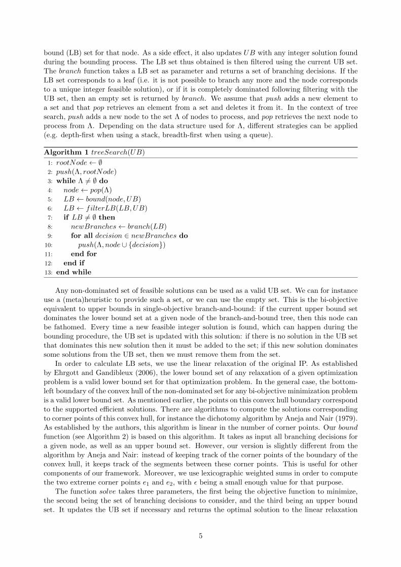
To any LB segment defined by points (x′, y′) and (x′′, y′′) we can associate the subset of objectivespace that it covers. This subset is the space dominated by any point on that segment, and

6

Obj. 1

Obj. 2

(x', y')

(x", y")

µ

Figure 1: Space dominated by a given segment between points (x′, y′) and (x′′, y′′), and local nadirpoint µ in objective space.

represents the possibility to find feasible solutions (x, y) in the space above the segment such thatx ≥ x′ and y ≥ y′′. Figure 1 depicts this space (shaded).

To each segment s, we associate a top-right corner (or local nadir) point µ of which coordinatesare valid single-objective upper bounds, one per objective, on the space dominated by this segment.In the most basic case the upper bounds can be arbitrarily large values. If the two extreme pointsof the Pareto front are known, we can deduce a tighter valid local nadir point from them. Similarly,we can associate to any LB set a valid local nadir point by considering, for each objective, themaximum value among the local nadir points of all segments in this LB set.

Here we note that we can partition the objective space, therefore the solution space, usingvalues for any of the two objectives, or any linear combination of both with positive weights (asis done in Stidsen et al. 2014). In our BIOBAB, we partition the objective space using differentintervals for the first objective, the union of these intervals covering the whole efficient objectivespace. A graphical interpretation is that the objective space can be split in vertical stripes.

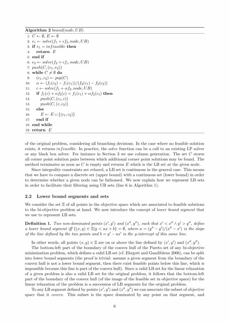
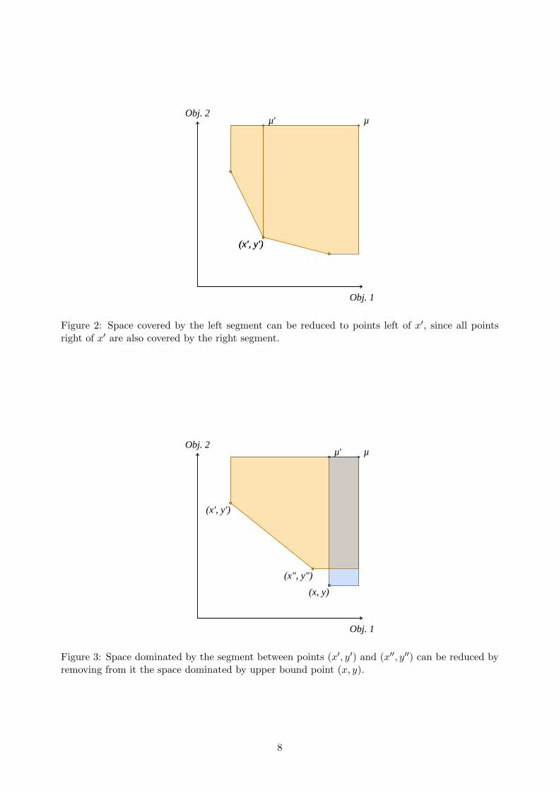
This allows us to improve the initial local nadir point for segments of a connected sequenceof segments: for any two segments connected by point (x′, y′), we cut from the space covered bythe left segment all points (x, y) such that x ≥ x′, since these points are also covered by the rightsegment. This is illustrated in Figure 2: the local nadir point for the segment left of x′ is now µ′.The local nadir point for the right-most segment is still µ.

By doing so, we partition the objective space covered by the LB set into different LB segmentswith associated local nadir points.

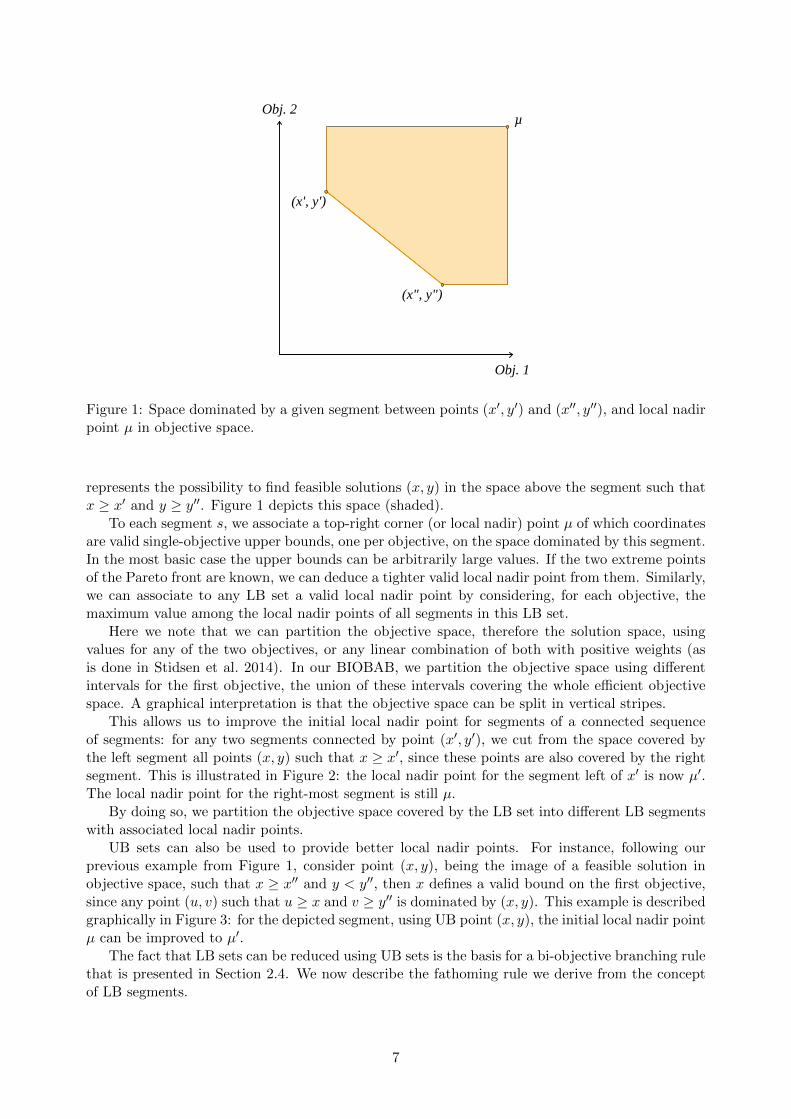
UB sets can also be used to provide better local nadir points. For instance, following ourprevious example from Figure 1, consider point (x, y), being the image of a feasible solution inobjective space, such that x ≥ x′′ and y < y′′, then x defines a valid bound on the first objective,since any point (u, v) such that u ≥ x and v ≥ y′′ is dominated by (x, y). This example is describedgraphically in Figure 3: for the depicted segment, using UB point (x, y), the initial local nadir pointµ can be improved to µ′.

The fact that LB sets can be reduced using UB sets is the basis for a bi-objective branching rulethat is presented in Section 2.4. We now describe the fathoming rule we derive from the conceptof LB segments.

7

Obj. 1

Obj. 2

(x', y')(x', y')

µ µ'

Figure 2: Space covered by the left segment can be reduced to points left of x′, since all pointsright of x′ are also covered by the right segment.

Obj. 1

Obj. 2

(x', y')

(x", y")

µ'

(x, y)

µ

Figure 3: Space dominated by the segment between points (x′, y′) and (x′′, y′′) can be reduced byremoving from it the space dominated by upper bound point (x, y).

8

2.3 Bound set comparisons and node fathoming

One major difficulty in previous approaches lies in the evaluation of the dominance of a given LBset by a given UB set. Multiple fathoming rules have been developed over the years (see Belottiet al. 2013, for the current state of the art). We now introduce the fathoming rule we use.

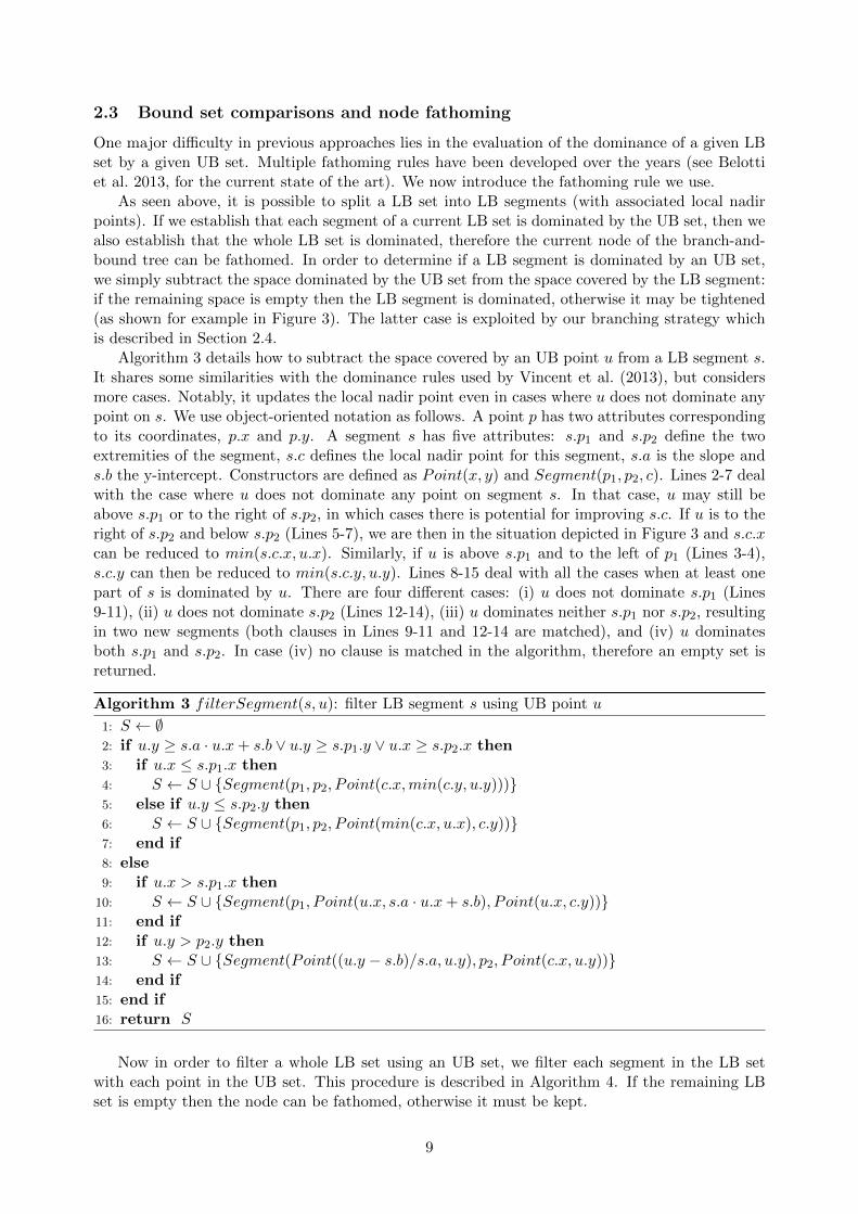
As seen above, it is possible to split a LB set into LB segments (with associated local nadirpoints). If we establish that each segment of a current LB set is dominated by the UB set, then wealso establish that the whole LB set is dominated, therefore the current node of the branch-and-bound tree can be fathomed. In order to determine if a LB segment is dominated by an UB set,we simply subtract the space dominated by the UB set from the space covered by the LB segment:if the remaining space is empty then the LB segment is dominated, otherwise it may be tightened(as shown for example in Figure 3). The latter case is exploited by our branching strategy whichis described in Section 2.4.

Algorithm 3 details how to subtract the space covered by an UB point u from a LB segment s.It shares some similarities with the dominance rules used by Vincent et al. (2013), but considersmore cases. Notably, it updates the local nadir point even in cases where u does not dominate anypoint on s. We use object-oriented notation as follows. A point p has two attributes correspondingto its coordinates, p.x and p.y. A segment s has five attributes: s.p1 and s.p2 define the twoextremities of the segment, s.c defines the local nadir point for this segment, s.a is the slope ands.b the y-intercept. Constructors are defined as Point(x, y) and Segment(p1, p2, c). Lines 2-7 dealwith the case where u does not dominate any point on segment s. In that case, u may still beabove s.p1 or to the right of s.p2, in which cases there is potential for improving s.c. If u is to theright of s.p2 and below s.p2 (Lines 5-7), we are then in the situation depicted in Figure 3 and s.c.xcan be reduced to min(s.c.x, u.x). Similarly, if u is above s.p1 and to the left of p1 (Lines 3-4),s.c.y can then be reduced to min(s.c.y, u.y). Lines 8-15 deal with all the cases when at least onepart of s is dominated by u. There are four different cases: (i) u does not dominate s.p1 (Lines9-11), (ii) u does not dominate s.p2 (Lines 12-14), (iii) u dominates neither s.p1 nor s.p2, resultingin two new segments (both clauses in Lines 9-11 and 12-14 are matched), and (iv) u dominatesboth s.p1 and s.p2. In case (iv) no clause is matched in the algorithm, therefore an empty set isreturned.

Algorithm 3 filterSegment(s, u): filter LB segment s using UB point u

1: S ← ∅2: if u.y ≥ s.a · u.x+ s.b ∨ u.y ≥ s.p1.y ∨ u.x ≥ s.p2.x then3: if u.x ≤ s.p1.x then4: S ← S ∪ Segment(p1, p2, Point(c.x,min(c.y, u.y)))5: else if u.y ≤ s.p2.y then6: S ← S ∪ Segment(p1, p2, Point(min(c.x, u.x), c.y))7: end if8: else9: if u.x > s.p1.x then

10: S ← S ∪ Segment(p1, Point(u.x, s.a · u.x+ s.b), Point(u.x, c.y))11: end if12: if u.y > p2.y then13: S ← S ∪ Segment(Point((u.y − s.b)/s.a, u.y), p2, Point(c.x, u.y))14: end if15: end if16: return S

Now in order to filter a whole LB set using an UB set, we filter each segment in the LB setwith each point in the UB set. This procedure is described in Algorithm 4. If the remaining LBset is empty then the node can be fathomed, otherwise it must be kept.

9

Algorithm 4 filterLB(LB,UB): filter LB set LB using UB set UB

1: S ← LB2: for all u ∈ UB do3: S′ ← ∅4: for all s ∈ S do5: S′ ← S′ ∪ filterSegment(s, u)6: end for7: S ← S′

8: end for9: return S

Obj. 1

Obj. 2

Obj. 1

Obj. 2

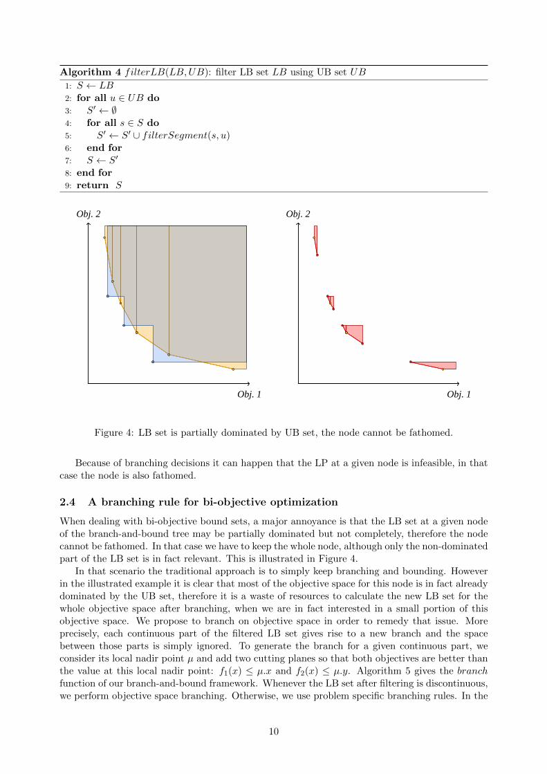
Figure 4: LB set is partially dominated by UB set, the node cannot be fathomed.

Because of branching decisions it can happen that the LP at a given node is infeasible, in thatcase the node is also fathomed.

2.4 A branching rule for bi-objective optimization

When dealing with bi-objective bound sets, a major annoyance is that the LB set at a given nodeof the branch-and-bound tree may be partially dominated but not completely, therefore the nodecannot be fathomed. In that case we have to keep the whole node, although only the non-dominatedpart of the LB set is in fact relevant. This is illustrated in Figure 4.

In that scenario the traditional approach is to simply keep branching and bounding. Howeverin the illustrated example it is clear that most of the objective space for this node is in fact alreadydominated by the UB set, therefore it is a waste of resources to calculate the new LB set for thewhole objective space after branching, when we are in fact interested in a small portion of thisobjective space. We propose to branch on objective space in order to remedy that issue. Moreprecisely, each continuous part of the filtered LB set gives rise to a new branch and the spacebetween those parts is simply ignored. To generate the branch for a given continuous part, weconsider its local nadir point µ and add two cutting planes so that both objectives are better thanthe value at this local nadir point: f1(x) ≤ µ.x and f2(x) ≤ µ.y. Algorithm 5 gives the branchfunction of our branch-and-bound framework. Whenever the LB set after filtering is discontinuous,we perform objective space branching. Otherwise, we use problem specific branching rules. In the

10

Algorithm 5 branch(LB)

1: N ← ∅2: if LB is discontinuous then3: for all continuous subset S ∈ LB do4: µ = Point(max

s∈S(s.c.x),max

s∈S(s.c.y))

5: decision ← (f1(x) ≤ µ.x ∧ f2(x) ≤ µ.y)6: N ← N ∪ decision7: end for8: else9: N ← problemSpecificBranching(LB)

10: end if11: return N

example of Figure 4, function branch generates four different branches.

2.5 Improvements based on the integrality of objective functions

When solving integer programs, in many cases, objective values of feasible integer solutions onlytake integer values. It is in practice almost always possible to use integer numbers. The reasonsinclude the fact that LP solvers have precision limitations, and that time-efficient floating-pointnumbers representations also have precision limitations. So rounding floating-point numbers isalmost always inevitable, and if numbers are rounded to d decimals then they may as well bemultiplied by 10d and considered integers. We note that this property is exploited by other methodsas well. For instance, the ε-constraint framework uses a known ε value which in our case wouldbe 1. In some cases, it is even possible to use values higher than 1, as long as these values arevalid: for instance if every coefficient for a given objective function is integer, then the greatestcommon divisor of these coefficients can be used as a valid value, just like it could be used in anε-constraint framework. For the sake of simplicity and without loss of generality, we consider inthe following that this valid value is 1. We now explore possibilities to speed up our bi-objectivebranch-and-bound by exploiting the fact that objective values of feasible solutions are alwaysinteger.

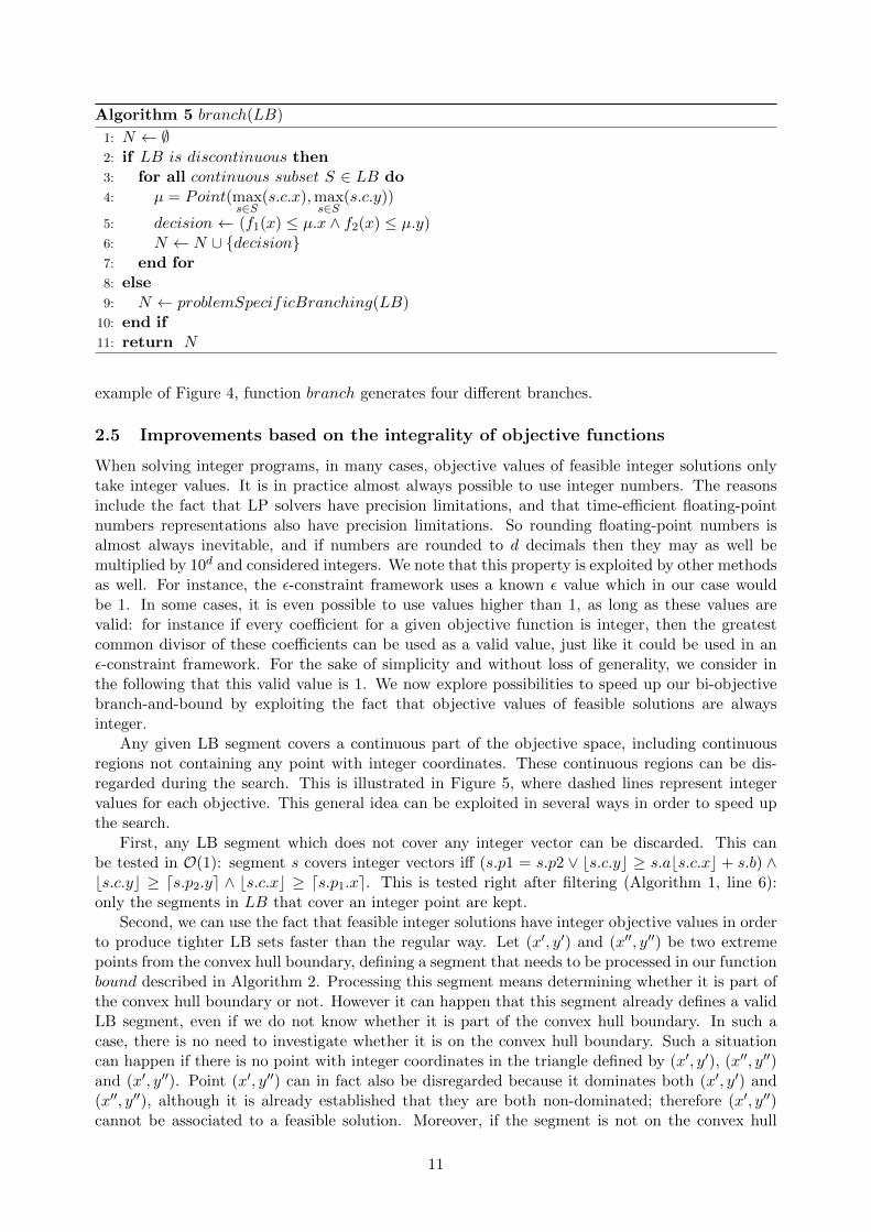
Any given LB segment covers a continuous part of the objective space, including continuousregions not containing any point with integer coordinates. These continuous regions can be dis-regarded during the search. This is illustrated in Figure 5, where dashed lines represent integervalues for each objective. This general idea can be exploited in several ways in order to speed upthe search.

First, any LB segment which does not cover any integer vector can be discarded. This canbe tested in O(1): segment s covers integer vectors iff (s.p1 = s.p2 ∨ bs.c.yc ≥ s.abs.c.xc + s.b) ∧bs.c.yc ≥ ds.p2.ye ∧ bs.c.xc ≥ ds.p1.xe. This is tested right after filtering (Algorithm 1, line 6):only the segments in LB that cover an integer point are kept.

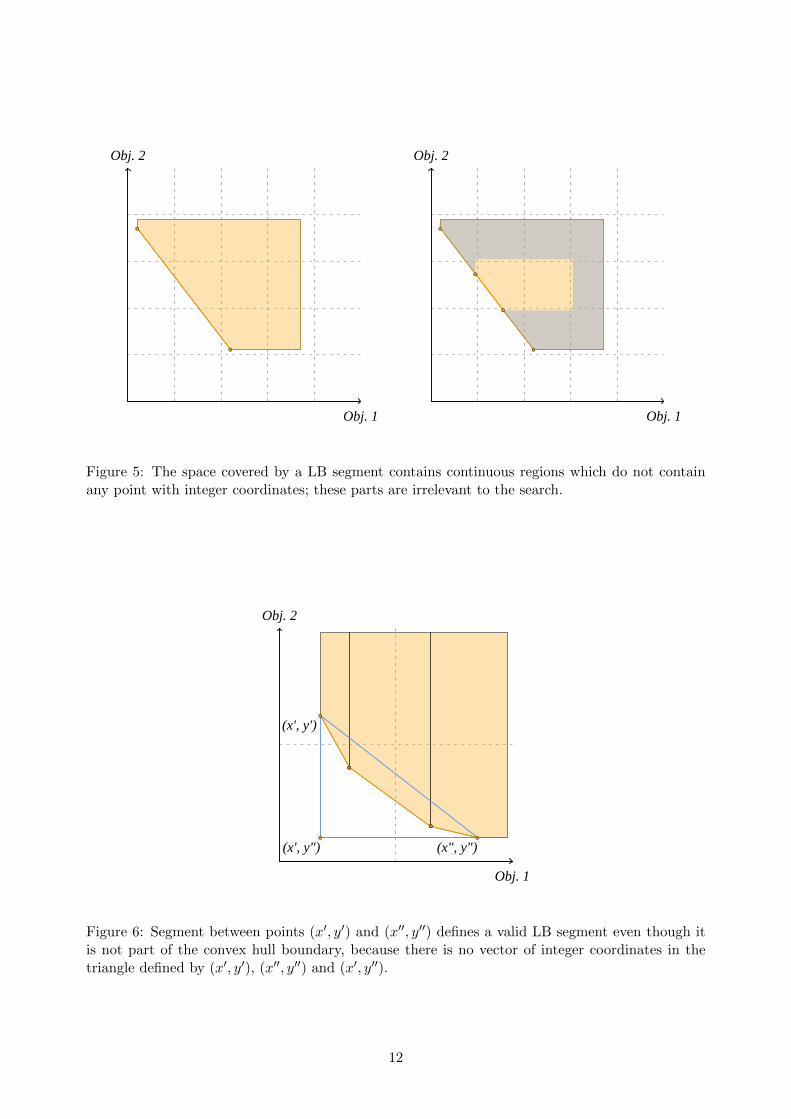
Second, we can use the fact that feasible integer solutions have integer objective values in orderto produce tighter LB sets faster than the regular way. Let (x′, y′) and (x′′, y′′) be two extremepoints from the convex hull boundary, defining a segment that needs to be processed in our functionbound described in Algorithm 2. Processing this segment means determining whether it is part ofthe convex hull boundary or not. However it can happen that this segment already defines a validLB segment, even if we do not know whether it is part of the convex hull boundary. In such acase, there is no need to investigate whether it is on the convex hull boundary. Such a situationcan happen if there is no point with integer coordinates in the triangle defined by (x′, y′), (x′′, y′′)and (x′, y′′). Point (x′, y′′) can in fact also be disregarded because it dominates both (x′, y′) and(x′′, y′′), although it is already established that they are both non-dominated; therefore (x′, y′′)cannot be associated to a feasible solution. Moreover, if the segment is not on the convex hull

11

Obj. 1

Obj. 2

Obj. 1

Obj. 2

Figure 5: The space covered by a LB segment contains continuous regions which do not containany point with integer coordinates; these parts are irrelevant to the search.

Obj. 1

Obj. 2

(x', y')

(x", y")(x', y")

Figure 6: Segment between points (x′, y′) and (x′′, y′′) defines a valid LB segment even though itis not part of the convex hull boundary, because there is no vector of integer coordinates in thetriangle defined by (x′, y′), (x′′, y′′) and (x′, y′′).

12

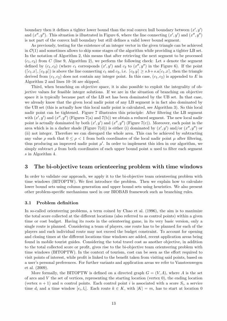
boundary then it defines a tighter lower bound than the real convex hull boundary between (x′, y′)and (x′′, y′′). This situation is illustrated in Figure 6, where the line connecting (x′, y′) and (x′′, y′′)is not part of the convex hull boundary but still defines a valid lower bound segment.

As previously, testing for the existence of an integer vector in the given triangle can be achievedin O(1) and sometimes allows to skip some stages of the algorithm while providing a tighter LB set.In the notation of Algorithm 2, this means that after retrieving the next segment to be processed(c1, c2) from C (line 9, Algorithm 2), we perform the following check: Let s denote the segmentdefined by (c1, c2) (where c1 corresponds (x′, y′) and c2 to (x′′, y′′) in the Figure 6). If the point(dc1.xe, dc2.ye) is above the line connecting c1 and c2, i.e. dc2.ye ≥ s.b+s.adc1.xe, then the trianglederived from (c1, c2) does not contain any integer point. In this case, (c1, c2) is appended to E inAlgorithm 2 and lines 10–16 are skipped.

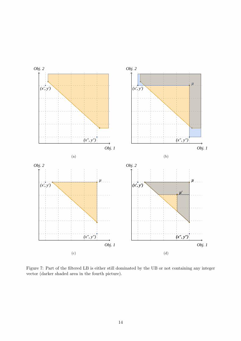
Third, when branching on objective space, it is also possible to exploit the integrality of ob-jective values for feasible integer solutions. If we are in the situation of branching on objectivespace it is typically because part of the LB set has been dominated by the UB set. In that case,we already know that the given local nadir point of any LB segment is in fact also dominated bythe UB set (this is actually how this local nadir point is calculated, see Algorithm 3). So this localnadir point can be tightened. Figure 7 illustrates this principle: After filtering the LB segmentwith (x′, y′) and (x′′, y′′) (Figures 7(a) and 7(b)) we obtain a reduced segment. The new local nadirpoint is actually dominated by both (x′, y′) and (x′′, y′′) (Figure 7(c)). Moreover, each point in thearea which is in a darker shade (Figure 7(d)) is either (i) dominated by (x′, y′) and/or (x′′, y′′) or(ii) not integer. Therefore we can disregard the whole area. This can be achieved by subtractingany value ρ such that 0 ≤ ρ < 1 from both coordinates of the local nadir point µ after filtering,thus producing an improved nadir point µ′. In order to implement this idea in our algorithm, wesimply subtract ρ from both coordinates of each upper bound point u used to filter each segments in Algorithm 4.

3 The bi-objective team orienteering problem with time windows

In order to validate our approach, we apply it to the bi-objective team orienteering problem withtime windows (BITOPTW). We first introduce the problem. Then we explain how to calculatelower bound sets using column generation and upper bound sets using heuristics. We also presentother problem-specific mechanisms used in our BIOBAB framework such as branching rules.

3.1 Problem definition

In so-called orienteering problems, a term coined by Chao et al. (1996), the aim is to maximizethe total score collected at the different locations (also referred to as control points) within a giventime or cost budget. Having its roots in the orienteering game, in its very basic version, only asingle route is planned. Considering a team of players, one route has to be planned for each of theplayers and each individual route may not exceed the budget constraint. To account for openingand closing times at the different locations time windows are added, recent application areas beingfound in mobile tourist guides. Considering the total travel cost as another objective, in additionto the total collected score or profit, gives rise to the bi-objective team orienteering problem withtime windows (BITOPTW). In the context of tourism, cost can be seen as the effort required tovisit points of interest, while profit is linked to the benefit taken from visiting said points, based ona user’s personal preferences. For further variants and application areas we refer to Vansteenwegenet al. (2009).

More formally, the BITOPTW is defined on a directed graph G = (V,A), where A is the setof arcs and V the set of vertices, representing the starting location (vertex 0), the ending location(vertex n + 1) and n control points. Each control point i is associated with a score Si, a servicetime di and a time window [ei, li]. Each route k ∈ K, with |K| = m, has to start at location 0

13

Obj. 1

Obj. 2

(x', y')

(x", y")

(a)

Obj. 1

Obj. 2

µ (x', y')

(x", y")

(b)

Obj. 1

Obj. 2

µ (x', y')

(x", y")

(c)

Obj. 1

Obj. 2

µ

µ'

(x', y')

(x", y")

µ

µ'

(x', y')

(x", y")

(d)

Figure 7: Part of the filtered LB is either still dominated by the UB or not containing any integervector (darker shaded area in the fourth picture).

14

and end at location n+ 1 and each arc (i, j) is associated with travel cost cij and travel time tij .The aim is to maximize the total collected score and to simultaneously minimize the total travelcost. Using binary decision variables zi ∈ 0, 1 equal to 1 if location i is visited and 0 otherwise,and yijk ∈ 0, 1 equal to 1 if arc (i, j) is traversed by route k and 0 otherwise, and continuousvariables Bik, denoting the beginning of service at i by route k, we formally define the BITOPTWas follows:

min∑k∈K

∑(i,j)∈A

cijyijk (1)

max∑

i∈V \0,n+1

Sizi (2)

subject to: ∑j∈V \0

y0jk = 1 ∀k ∈ K (3)

∑i∈V \n+1

yi,n+1,k = 1 ∀k ∈ K (4)

∑k∈K

∑j∈V \n+1

yjik = zi ∀i ∈ V \ 0, n+ 1 (5)

∑j∈V \n+1

yjik −∑

j∈V \0

yijk = 0 ∀k ∈ K, i ∈ V \ 0, n+ 1 (6)

(Bik + di + tij)yijk ≤ Bjk ∀k ∈ K, (i, j) ∈ A (7)

ei ≤ Bik ≤ li ∀k ∈ K, i ∈ V (8)

yijk ∈ 0, 1 ∀k ∈ K, (i, j) ∈ A (9)

zi ∈ 0, 1 ∀i ∈ V \ 0, n+ 1 (10)

Objective function (1) minimizes the total routing costs while objective function (2) maximizesthe total collected profit. Constraints (3) and (4) make sure that each route starts at the definedstarting point and ends at the correct ending point. Constraints (5) link the binary decisionvariables and (6) ensure connectivity for visited nodes. Constraints (7) set the time variablesand (8) make sure that time windows are respected. We note that constraints (7) are not linearbut they can easily be linearized using big M terms.

We solve the BITOPTW with the proposed BIOBAB, where lower bound sets are generatedby means of column generation. This is described next.

3.2 Lower bound sets: column generation

Since state-of-the-art exact methods for single-objective routing problems mostly rely on columngeneration based techniques (see, e.g. Baldacci et al. 2012), we also generate lower bound sets forthe BITOPTW by means of column generation.

Let pr denote the total score or profit achieved by route r, cr the total travel cost of route r,and let air indicate whether location i is visited by route r (air = 1) or not (air = 0). Using binaryvariables xr equal to 1 if route r is selected from the set Ω of all feasible routes, the BITOPTWcan also be formulated as a path-based model:

f1 = min∑r∈Ω

crxr (11)

f2 = max∑r∈Ω

prxr (12)

15

∑r∈Ω

airxr ≤ 1 ∀i ∈ N (13)∑r∈Ω

xr = m (14)

xr ∈ 0, 1 ∀r ∈ Ω. (15)

Relaxing integrality requirements on the xr variables, we replace constraints (15) with:

xr ≥ 0 ∀r ∈ Ω (16)

We also combine the two objective functions into a weighted sum (w1 and w2 giving the respectivenon-negative weights):

min∑r∈Ω

(w1cr − w2pr)xr (17)

We thus obtain a single objective linear problem that can be solved by means of column generation,which allows us to compute LB sets using Algorithm 2. In column generation (see, e.g. Desrosiersand Lubbecke 2005), in each iteration a subset of promising columns is generated and appended tothe restricted set of columns Ω′ and the single objective linear program is re-solved on Ω′. Columngeneration continues as long as new promising columns exist. Otherwise, the optimal solution hasbeen found (i.e. in that case, the optimal solution of the single objective linear program on Ω′

is also the optimal solution of the single objective linear program on Ω). Promising columns areidentified using dual information. Let πi denote the dual variable associated with constraint (13)for a given i and α the dual variable associated with constraint (14), the pricing subproblem wehave to solve corresponds to:

min w1cr − w2pr −∑i∈N

airπi − α (18)

subject to constraints (3)–(10), omitting subscript k. It is an elementary shortest path problemwith resource constraints that can be solved by means of a labeling algorithm (cf. Feillet et al.2004). In our labeling algorithm, a label carries the following information: the node the labelis associated with, the time consumption until that node, the reduced cost so far, which nodeshave been visited along the path leading to the node, and a pointer to the parent label. In orderto compute the reduced cost of the path associated with a given label, we use a reduced costmatrix that is generated before the labeling algorithm is called. The reduced cost of arc (i, j)is cij = w1cij − w2Si − πi, where if i = 0, πi is replaced by α. Since the aim of this paper isnot to investigate the most efficient pricing algorithm, we refrain from adopting all enhancementsproposed in the literature (e.g., Righini and Salani 2009).

Note that during the execution of BIOBAB we keep all previously generated columns in thecolumn pool. We only temporarily deactivate those columns that are incompatible with currentbranching decisions. When branching on objective space, it can happen that the current pool ofcolumns does not allow to produce a feasible solution. This can be due to two reasons: either(i) because there exists no feasible solution to the current problem or (ii) because there existsa feasible solution but it cannot be reached with the currently available columns. In order tofix this issue and guarantee feasibility, we use a dummy column which allows to satisfy everyconstraint from the current problem, including the branching decisions described in Section 3.4.This column covers all mandatory control points, does not cover any forbidden control point, usesall the available vehicles, has a cost inferior to the maximum allowed cost and a profit superior tothe minimum allowed profit. Using this column is penalized in the objective function, so that thecolumn generation procedure converges to feasible solutions that do not use the dummy column.Assuming the variable associated to this dummy column is xD, the objective function described inEquation (17) is modified as follows:

16

min∑r∈Ω

(w1cr − w2pr)xr +MxD, (19)

where M is an arbitrarily large number. The dummy column is only activated when no feasiblesolution can be found, and it is systematically deactivated after column generation converges. Atthis point, if xD has a strictly positive value then there does not exist a feasible solution thatsatisfies all the branching decisions.

3.3 Upper bound sets: multi-directional local search

Using starting upper bound sets has two advantages: uninteresting branches of the search tree maybe pruned earlier and valid starting columns for our lower bound computations are available. Forthe BITOPTW we generate upper bound sets by means of multi-directional local search (MDLS).MDLS has been proposed in Tricoire (2012) where it is shown that MDLS is able to providecompetitive results for the multi-objective multi-dimensional knapsack problem, the bi-objectiveset packing problem and the bi-objective orienteering problem. It obtains approximations of thePareto frontier of either comparable or improved quality. Its main idea is to use several differentlocal search procedures, each considering only one of the objectives. At each iteration, a solution isselected from the current set of non-dominated solutions. Then, local search is performed on thissolution for each of the objectives in turn. Therefore, each call to a local search algorithm aims ata different “direction”. Using the thus produced new solutions, the non-dominated set is updatedand the next iteration is performed.

In this work we use large neighborhood search (LNS) (Shaw 1998, Ropke and Pisinger 2006)as single-objective local search. The LNS we apply works as follows. In every iteration, first, thenumber of nodes to be removed from the current solution is randomly chosen from [1, 0.4ν], whereν gives the number of currently visited nodes. Then, a destroy and a repair operator are chosenrandomly and applied to the current solution. Destroy operators remove control points from thesolution while repair operators insert control points into routes. In terms of destroy operators, weuse a greedy and a random operator. In terms of repair operators, we use a greedy, a random and a“nil” operator. The greedy operators choose the points that help to improve the currently employedobjective function the most or to deteriorate it the least. The random operators randomly selectthe points to be removed or inserted. The “nil” operator does not do anything. It is used toallow the application of a destroy operator without subsequent repairing, which leads to improvedsolutions when optimizing cost. In the repair phase, once a point has been selected for insertion,it is inserted at the cheapest position in terms of travel cost. The random destroy – random repairoperator pair is not employed.

In addition, we add noise to the greedy operators by multiplying the selection value (either thedifference in terms of profit or cost, depending on the objective being currently optimized) by afactor randomly chosen in [0.4, 1].

3.4 Tree search

We now explain how the search tree is constructed, i.e. which branching rules are used, as wellas how it is explored. In terms of tree exploration strategy, we use breadth-first search. Wealso implemented depth-first as well as best-first strategies, where the total area covered by alower bound set is used as score for the best-first strategy. In a preliminary set of experimentsneither of these performed significantly worse than breadth-first, but breadth-first still providedthe best performance overall. In terms of branching rules, whenever the lower bound after filteringis discontinuous, we perform objective space branching (see Section 2.4). Since objective spacebranching involves setting bounds on both objectives, we include such constraints right from thestart (initially setting the respective bounds to infinity) and later update them according to the

17

branching decisions. In order to properly incorporate dual information from these two constraintsinto the subproblem, we modify the reduced cost matrix accordingly. In the case where the lowerbound is not discontinuous, we either branch on control points or on arcs (Line 9 in Algorithm 5):First, we check if a control point is visited a fractional number of times. Since each lower boundrepresents a set of solutions, the number of times a control point is visited may take different valueswithin the same LB set. In order to select a control point to branch on, we consider the extremepoints of the boundary of the convex hull defining the current LB set, each of these being associatedto a different solution. We then average the number of visits for each control point over this setof solutions. The control point with the average number of visits closest to 0.5 is then selectedfor branching. In the case where each control point is visited 0 or 1 time on average, we checkfor arcs that are traversed a fractional number of times on average, following the same procedure.Branching on control points can be achieved by modifying constraint (13) in the master problem.In order to force the visit of control point i, this constraint becomes

∑r∈Ω

airxr ≥ 1. In order to

forbid the visit of i, this constraint becomes∑r∈Ω

airxr ≤ 0. As is usual in branch-and-price for

routing, branching on arcs involves adding constraints to the subproblem.

4 Experimental study

All algorithms are implemented in C++, compiled with g++ version 4.6.2 and run on an 2.67 GHzIntel Xeon CPU. We use ILOG Cplex 12.5 to solve linear programs in the column generation. Werestrict Cplex to a single thread and set the parameter EpRHS to 10−7 in order to avoid numericalstability issues. For MDLS, we use the code available at http://prolog.univie.ac.at/research/MDLSand extend it, as explained above, to tackle the BITOPTW. All the code used in our experimentswill be available online at http://prolog.univie.ac.at/research/BIOBAB.

To test our algorithms, we use instances from the data set of Righini and Salani (2009). In thisdata set, orienteering instances are derived from 29 instances for the vehicle routing problem withtime windows (VRPTW) (Solomon 1987) and from 10 instances for the multi-depot periodic vehiclerouting problem (MDPVRP) (Cordeau et al. 1997). From those derived from VRPTW instances,we use instance c101 100 (clustered locations), r101 100 (randomly spread locations) and rc101 100(mix of clustered and random locations). From those derived from MDPVRP instances, we useinstance pr01 (randomly spread locations). To obtain smaller instances, we consider the firstn = 15, 20, 25, 30 control points and m = 1, 2, 3, 4 vehicles. Distances are given with 2-digitprecision in the original instances, so we multiply them by 100 and only work with integer numbers.

4.1 Performance of the bi-objective branch-and-bound

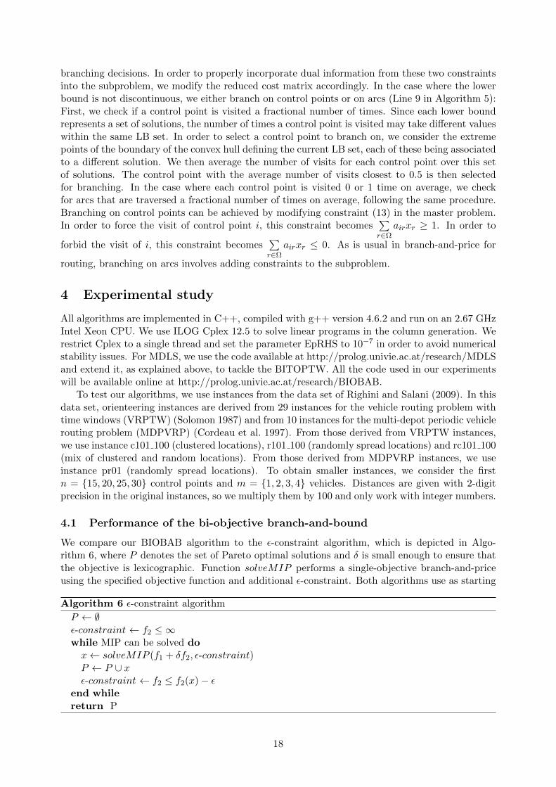
We compare our BIOBAB algorithm to the ε-constraint algorithm, which is depicted in Algo-rithm 6, where P denotes the set of Pareto optimal solutions and δ is small enough to ensure thatthe objective is lexicographic. Function solveMIP performs a single-objective branch-and-priceusing the specified objective function and additional ε-constraint. Both algorithms use as starting

Algorithm 6 ε-constraint algorithm

P ← ∅ε-constraint ← f2 ≤ ∞while MIP can be solved dox← solveMIP (f1 + δf2, ε-constraint)P ← P ∪ xε-constraint ← f2 ≤ f2(x)− ε

end whilereturn P

18

BIOBAB ε-constraint

n #solved tB < tεtεtB> 1.5 tε

tB> 3 #solved tε < tB

tBtε> 1.5 tB

tε> 3

15 16 3 0 0 16 13 1 020 16 1 1 1 16 15 4 025 14 8 2 1 14 6 0 030 13 7 2 0 13 6 0 035 11 6 2 1 11 5 0 0

Total 70 25 7 3 70 45 5 0

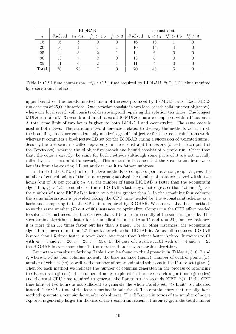
Table 1: CPU time comparison. “tB”: CPU time required by BIOBAB. “tε”: CPU time requiredby ε-constraint method.

upper bound set the non-dominated union of the sets produced by 10 MDLS runs. Each MDLSrun consists of 25,000 iterations. One iteration consists in two local search calls (one per objective),where one local search call consists of destroying and repairing the solution ten times. The longestMDLS run takes 2.13 seconds and in all cases all 10 MDLS runs are completed within 15 seconds.A total time limit of two hours is given to both BIOBAB and ε-constraint. The same code isused in both cases. There are only two differences, related to the way the methods work. First,the bounding procedure considers only one lexicographic objective for the ε-constraint framework,whereas it computes a bi-objective LB set for the BIOBAB (using a succession of weighted sums).Second, the tree search is called repeatedly in the ε-constraint framework (once for each point ofthe Pareto set), whereas the bi-objective branch-and-bound consists of a single run. Other thanthat, the code is exactly the same for both methods (although some parts of it are not actuallycalled by the ε-constraint framework). This means for instance that the ε-constraint frameworkbenefits from the existing UB set and can use it to fathom subtrees.

In Table 1 the CPU effort of the two methods is compared per instance group: n gives thenumber of control points of the instance group; #solved the number of instances solved within twohours (out of 16 per group); tB < tε the number of times BIOBAB is faster than the ε-constraintalgorithm, tε

tB> 1.5 the number of times BIOBAB is faster by a factor greater than 1.5; and tε

tB> 3

the number of times BIOBAB is faster by a factor greater than 3. In the remaining four columnsthe same information is provided taking the CPU time needed by the ε-constraint scheme as abasis and comparing it to the CPU time required by BIOBAB. We observe that both methodssolve the same number (70 out of 80) instances to optimality. Comparing the CPU effort neededto solve these instances, the table shows that CPU times are usually of the same magnitude. Theε-constraint algorithm is faster for the smallest instances (n = 15 and n = 20), for five instancesit is more than 1.5 times faster but less than 3 times. For all other instances, the ε-constraintalgorithm is never more than 1.5 times faster while the BIOBAB is. Across all instances BIOBABis more than 1.5 times faster in seven cases, and more than 3 times faster in three (instances rc101with m = 4 and n = 20, n = 25, n = 35). In the case of instance rc101 with m = 4 and n = 25the BIOBAB is even more than 10 times faster than the ε-constraint algorithm.

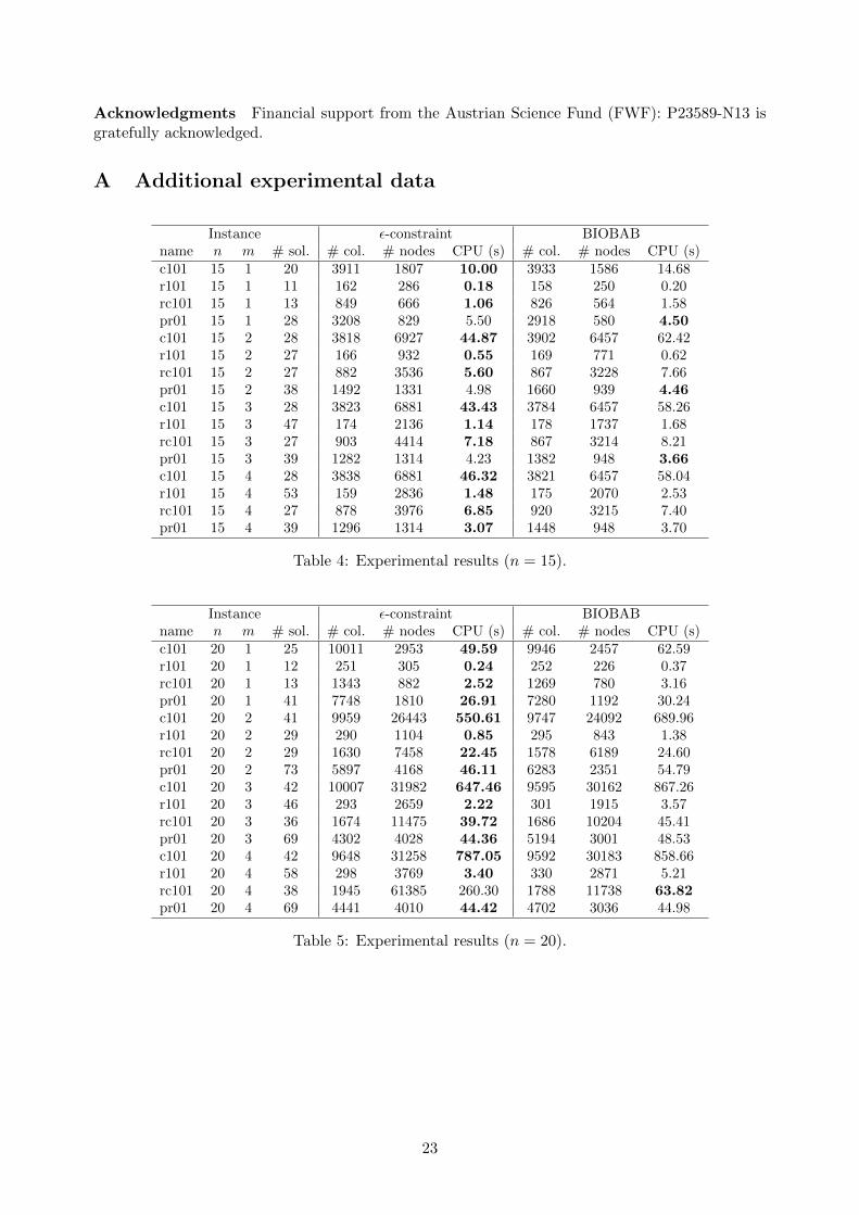
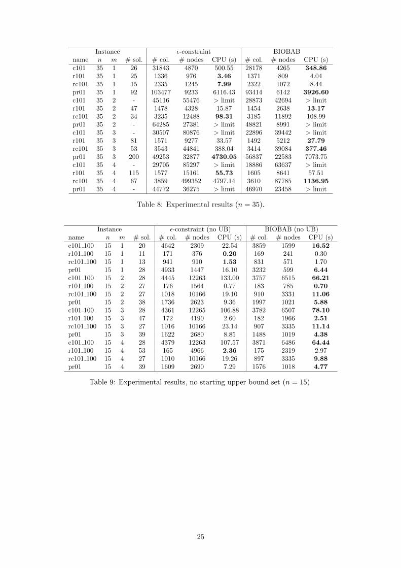
Per instance results underlying Table 1 can be found in the Appendix in Tables 4, 5, 6, 7 and8, where the first four columns indicate the base instance (name), number of control points (n),number of vehicles (m) as well as the number of non-dominated solutions in the Pareto set (# sol.).Then for each method we indicate the number of columns generated in the process of producingthe Pareto set (# col.), the number of nodes explored in the tree search algorithms (# nodes)and the total CPU time required to generate the Pareto set, in seconds (CPU (s)). If the CPUtime limit of two hours is not sufficient to generate the whole Pareto set, “> limit” is indicatedinstead. The CPU time of the fastest method is bold-faced. These tables show that, usually, bothmethods generate a very similar number of columns. The difference in terms of the number of nodesexplored is generally larger (in the case of the ε-constraint scheme, this entry gives the total number

19

BIOBAB (no UB) ε-constraint (no UB)

n #solved tB < tεtεtB> 1.5 tε

tB> 3 #solved tε < tB

tBtε> 1.5 tB

tε> 3

15 16 13 9 0 16 3 0 020 16 14 11 5 16 2 0 025 14 14 7 2 13 0 0 030 13 12 9 2 11 1 0 035 10 9 6 2 7 1 0 0

Total 69 62 42 11 63 7 0 0

Table 2: CPU time comparison, no starting upper bound set. “tB”: CPU time required byBIOBAB. “tε”: CPU time required by ε-constraint method.

of nodes explored across all single objective branch-and-bound calls). Fewer nodes are explored inthe BIOBAB, and much fewer nodes in those cases where BIOBAB provides much shorter CPUtimes. There is a trade-off relationship between the time spent on the evaluation of each node andthe number of nodes that can be explored in the same CPU time. Since the evaluation of eachnode is more costly in the BIOBAB than in the single objective branch-and-bound algorithm ofthe ε-constraint scheme, this result is expected and it indicates that the proposed ingredients helpto keep the tree size small. They are evaluated in further detail later on.

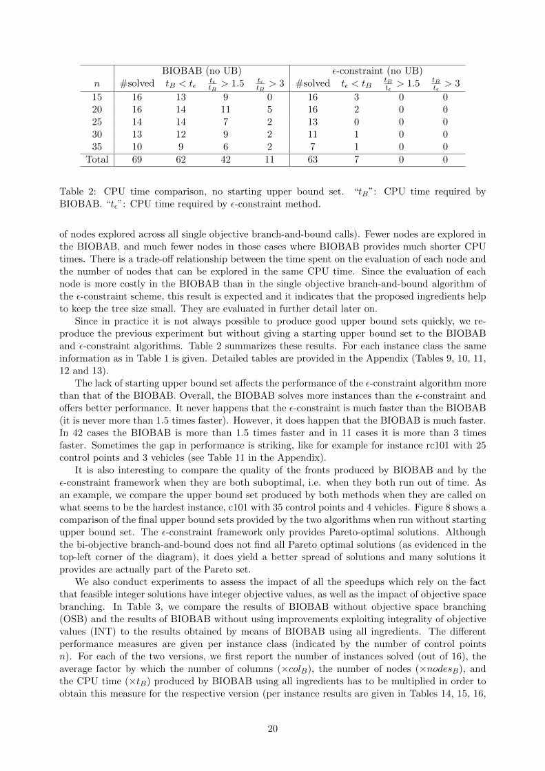
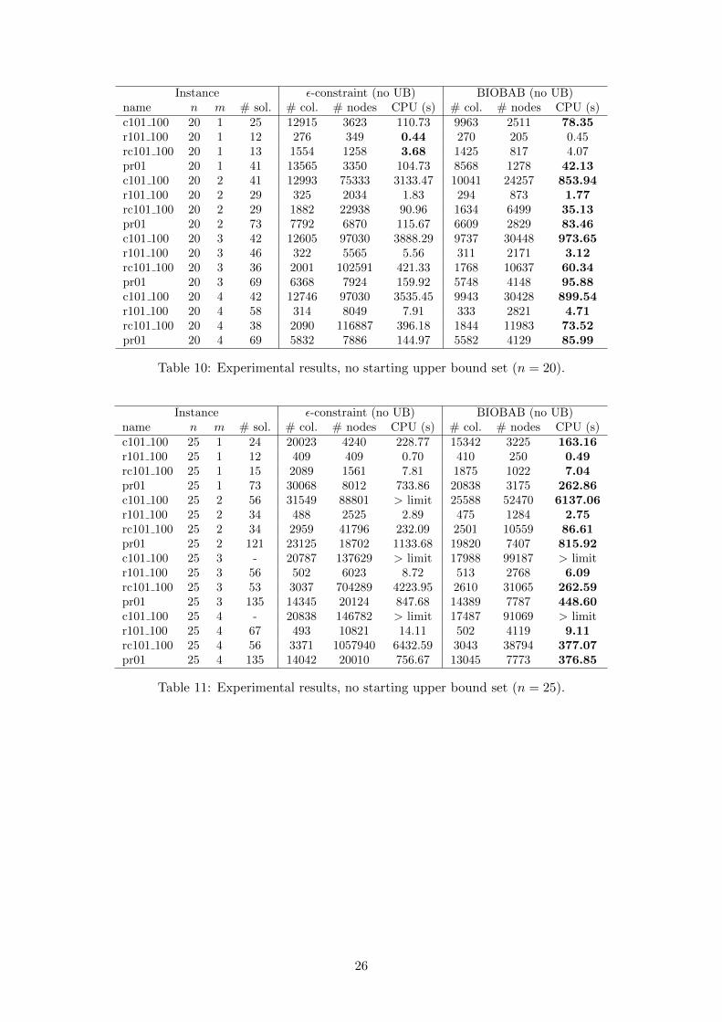
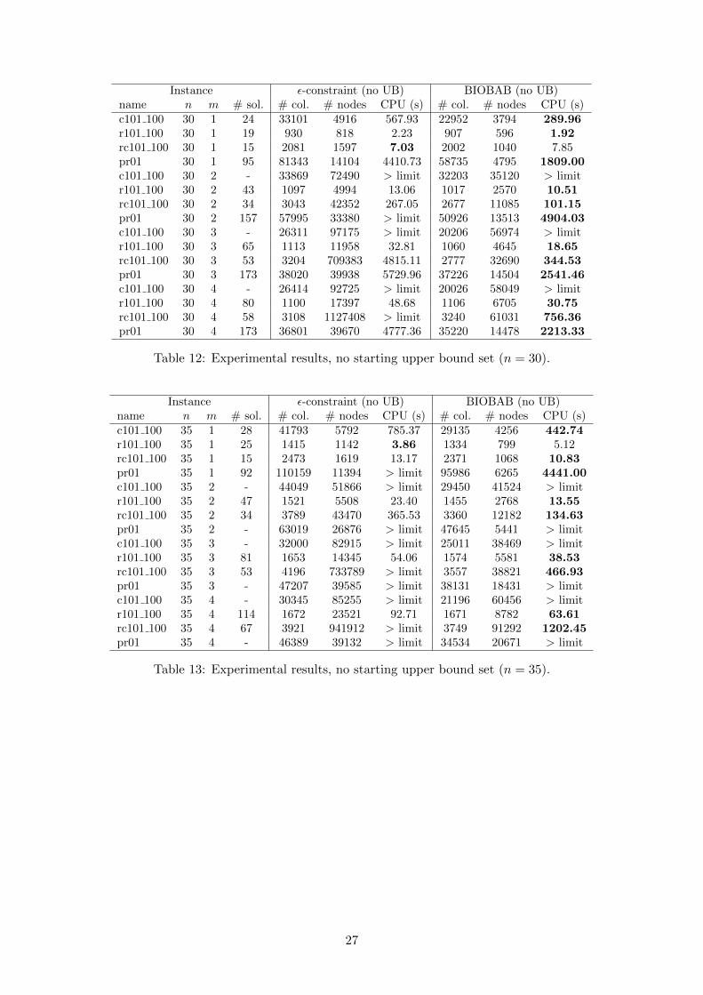
Since in practice it is not always possible to produce good upper bound sets quickly, we re-produce the previous experiment but without giving a starting upper bound set to the BIOBABand ε-constraint algorithms. Table 2 summarizes these results. For each instance class the sameinformation as in Table 1 is given. Detailed tables are provided in the Appendix (Tables 9, 10, 11,12 and 13).

The lack of starting upper bound set affects the performance of the ε-constraint algorithm morethan that of the BIOBAB. Overall, the BIOBAB solves more instances than the ε-constraint andoffers better performance. It never happens that the ε-constraint is much faster than the BIOBAB(it is never more than 1.5 times faster). However, it does happen that the BIOBAB is much faster.In 42 cases the BIOBAB is more than 1.5 times faster and in 11 cases it is more than 3 timesfaster. Sometimes the gap in performance is striking, like for example for instance rc101 with 25control points and 3 vehicles (see Table 11 in the Appendix).

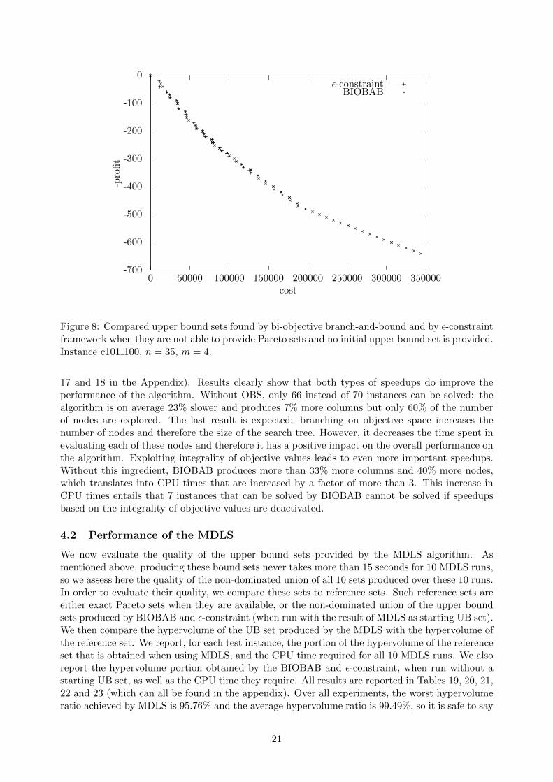
It is also interesting to compare the quality of the fronts produced by BIOBAB and by theε-constraint framework when they are both suboptimal, i.e. when they both run out of time. Asan example, we compare the upper bound set produced by both methods when they are called onwhat seems to be the hardest instance, c101 with 35 control points and 4 vehicles. Figure 8 shows acomparison of the final upper bound sets provided by the two algorithms when run without startingupper bound set. The ε-constraint framework only provides Pareto-optimal solutions. Althoughthe bi-objective branch-and-bound does not find all Pareto optimal solutions (as evidenced in thetop-left corner of the diagram), it does yield a better spread of solutions and many solutions itprovides are actually part of the Pareto set.

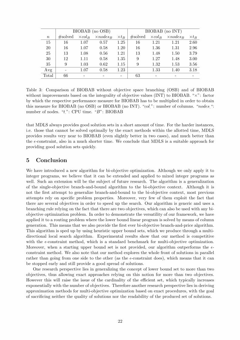
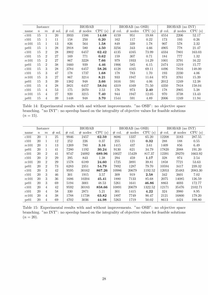
We also conduct experiments to assess the impact of all the speedups which rely on the factthat feasible integer solutions have integer objective values, as well as the impact of objective spacebranching. In Table 3, we compare the results of BIOBAB without objective space branching(OSB) and the results of BIOBAB without using improvements exploiting integrality of objectivevalues (INT) to the results obtained by means of BIOBAB using all ingredients. The differentperformance measures are given per instance class (indicated by the number of control pointsn). For each of the two versions, we first report the number of instances solved (out of 16), theaverage factor by which the number of columns (×colB), the number of nodes (×nodesB), andthe CPU time (×tB) produced by BIOBAB using all ingredients has to be multiplied in order toobtain this measure for the respective version (per instance results are given in Tables 14, 15, 16,

20

-700

-600

-500

-400

-300

-200

-100

0

0 50000 100000 150000 200000 250000 300000 350000

-pro

fit

cost

ε-constraintBIOBAB

Figure 8: Compared upper bound sets found by bi-objective branch-and-bound and by ε-constraintframework when they are not able to provide Pareto sets and no initial upper bound set is provided.Instance c101 100, n = 35, m = 4.

17 and 18 in the Appendix). Results clearly show that both types of speedups do improve theperformance of the algorithm. Without OBS, only 66 instead of 70 instances can be solved: thealgorithm is on average 23% slower and produces 7% more columns but only 60% of the numberof nodes are explored. The last result is expected: branching on objective space increases thenumber of nodes and therefore the size of the search tree. However, it decreases the time spent inevaluating each of these nodes and therefore it has a positive impact on the overall performance onthe algorithm. Exploiting integrality of objective values leads to even more important speedups.Without this ingredient, BIOBAB produces more than 33% more columns and 40% more nodes,which translates into CPU times that are increased by a factor of more than 3. This increase inCPU times entails that 7 instances that can be solved by BIOBAB cannot be solved if speedupsbased on the integrality of objective values are deactivated.

4.2 Performance of the MDLS

We now evaluate the quality of the upper bound sets provided by the MDLS algorithm. Asmentioned above, producing these bound sets never takes more than 15 seconds for 10 MDLS runs,so we assess here the quality of the non-dominated union of all 10 sets produced over these 10 runs.In order to evaluate their quality, we compare these sets to reference sets. Such reference sets areeither exact Pareto sets when they are available, or the non-dominated union of the upper boundsets produced by BIOBAB and ε-constraint (when run with the result of MDLS as starting UB set).We then compare the hypervolume of the UB set produced by the MDLS with the hypervolume ofthe reference set. We report, for each test instance, the portion of the hypervolume of the referenceset that is obtained when using MDLS, and the CPU time required for all 10 MDLS runs. We alsoreport the hypervolume portion obtained by the BIOBAB and ε-constraint, when run without astarting UB set, as well as the CPU time they require. All results are reported in Tables 19, 20, 21,22 and 23 (which can all be found in the appendix). Over all experiments, the worst hypervolumeratio achieved by MDLS is 95.76% and the average hypervolume ratio is 99.49%, so it is safe to say

21

BIOBAB (no OSB) BIOBAB (no INT)n #solved ×colB ×nodesB ×tB #solved ×colB ×nodesB ×tB15 16 1.07 0.57 1.25 16 1.21 1.21 2.6020 16 1.07 0.58 1.20 16 1.36 1.31 2.9625 13 1.08 0.56 1.21 13 1.48 1.50 3.7930 12 1.11 0.58 1.35 9 1.27 1.48 3.0035 9 1.03 0.62 1.15 9 1.32 1.53 3.56

Avg - 1.07 0.58 1.23 1.33 1.40 3.18

Total 66 - - - 63 - - -

Table 3: Comparison of BIOBAB without objective space branching (OSB) and of BIOBABwithout improvements based on the integrality of objective values (INT) to BIOBAB. “×”: factorby which the respective performance measure for BIOBAB has to be multiplied in order to obtainthis measure for BIOBAB (no OSB) or BIOBAB (no INT). “col.”: number of columns. “nodes.“:number of nodes. “t.”: CPU time. “B”: BIOBAB

that MDLS always provides good solution sets in a short amount of time. For the harder instances,i.e. those that cannot be solved optimally by the exact methods within the allotted time, MDLSprovides results very near to BIOBAB (even slightly better in two cases), and much better thanthe ε-constraint, also in a much shorter time. We conclude that MDLS is a suitable approach forproviding good solution sets quickly.

5 Conclusion

We have introduced a new algorithm for bi-objective optimization. Although we only apply it tointeger programs, we believe that it can be extended and applied to mixed integer programs aswell. Such an extension will be the subject of future research. The algorithm is a generalizationof the single-objective branch-and-bound algorithm to the bi-objective context. Although it isnot the first attempt to generalize branch-and-bound to the bi-objective context, most previousattempts rely on specific problem properties. Moreover, very few of them exploit the fact thatthere are several objectives in order to speed up the search. Our algorithm is generic and uses abranching rule relying on the fact that there are two objectives, which can also be used with any bi-objective optimization problem. In order to demonstrate the versatility of our framework, we haveapplied it to a routing problem where the lower bound linear program is solved by means of columngeneration. This means that we also provide the first ever bi-objective branch-and-price algorithm.This algorithm is sped up by using heuristic upper bound sets, which we produce through a multi-directional local search algorithm. Experimental results show that our method is competitivewith the ε-constraint method, which is a standard benchmark for multi-objective optimization.Moreover, when a starting upper bound set is not provided, our algorithm outperforms the ε-constraint method. We also note that our method explores the whole front of solutions in parallelrather than going from one side to the other (as the ε-constraint does), which means that it canbe stopped early and still provide a good spread of solutions.

One research perspective lies in generalizing the concept of lower bound set to more than twoobjectives, thus allowing exact approaches relying on this notion for more than two objectives.However this will raise the issue of the cardinality of the efficient set, which typically increasesexponentially with the number of objectives. Therefore another research perspective lies in derivingapproximation methods for multi-objective optimization based on exact procedures, with the goalof sacrificing neither the quality of solutions nor the readability of the produced set of solutions.

22

Acknowledgments Financial support from the Austrian Science Fund (FWF): P23589-N13 isgratefully acknowledged.

A Additional experimental data

Instance ε-constraint BIOBABname n m # sol. # col. # nodes CPU (s) # col. # nodes CPU (s)c101 15 1 20 3911 1807 10.00 3933 1586 14.68r101 15 1 11 162 286 0.18 158 250 0.20rc101 15 1 13 849 666 1.06 826 564 1.58pr01 15 1 28 3208 829 5.50 2918 580 4.50c101 15 2 28 3818 6927 44.87 3902 6457 62.42r101 15 2 27 166 932 0.55 169 771 0.62rc101 15 2 27 882 3536 5.60 867 3228 7.66pr01 15 2 38 1492 1331 4.98 1660 939 4.46c101 15 3 28 3823 6881 43.43 3784 6457 58.26r101 15 3 47 174 2136 1.14 178 1737 1.68rc101 15 3 27 903 4414 7.18 867 3214 8.21pr01 15 3 39 1282 1314 4.23 1382 948 3.66c101 15 4 28 3838 6881 46.32 3821 6457 58.04r101 15 4 53 159 2836 1.48 175 2070 2.53rc101 15 4 27 878 3976 6.85 920 3215 7.40pr01 15 4 39 1296 1314 3.07 1448 948 3.70

Table 4: Experimental results (n = 15).

Instance ε-constraint BIOBABname n m # sol. # col. # nodes CPU (s) # col. # nodes CPU (s)c101 20 1 25 10011 2953 49.59 9946 2457 62.59r101 20 1 12 251 305 0.24 252 226 0.37rc101 20 1 13 1343 882 2.52 1269 780 3.16pr01 20 1 41 7748 1810 26.91 7280 1192 30.24c101 20 2 41 9959 26443 550.61 9747 24092 689.96r101 20 2 29 290 1104 0.85 295 843 1.38rc101 20 2 29 1630 7458 22.45 1578 6189 24.60pr01 20 2 73 5897 4168 46.11 6283 2351 54.79c101 20 3 42 10007 31982 647.46 9595 30162 867.26r101 20 3 46 293 2659 2.22 301 1915 3.57rc101 20 3 36 1674 11475 39.72 1686 10204 45.41pr01 20 3 69 4302 4028 44.36 5194 3001 48.53c101 20 4 42 9648 31258 787.05 9592 30183 858.66r101 20 4 58 298 3769 3.40 330 2871 5.21rc101 20 4 38 1945 61385 260.30 1788 11738 63.82pr01 20 4 69 4441 4010 44.42 4702 3036 44.98

Table 5: Experimental results (n = 20).

23

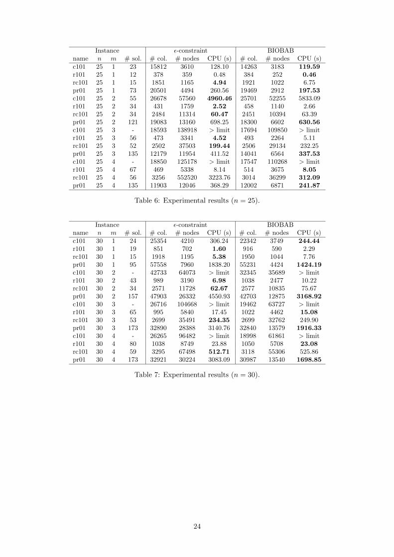
Instance ε-constraint BIOBABname n m # sol. # col. # nodes CPU (s) # col. # nodes CPU (s)c101 25 1 23 15812 3610 128.10 14263 3183 119.59r101 25 1 12 378 359 0.48 384 252 0.46rc101 25 1 15 1851 1165 4.94 1921 1022 6.75pr01 25 1 73 20501 4494 260.56 19469 2912 197.53c101 25 2 55 26678 57560 4960.46 25701 52255 5833.09r101 25 2 34 431 1759 2.52 458 1140 2.66rc101 25 2 34 2484 11314 60.47 2451 10394 63.39pr01 25 2 121 19083 13160 698.25 18300 6602 630.56c101 25 3 - 18593 138918 > limit 17694 109850 > limitr101 25 3 56 473 3341 4.52 493 2264 5.11rc101 25 3 52 2502 37503 199.44 2506 29134 232.25pr01 25 3 135 12179 11954 411.52 14041 6564 337.53c101 25 4 - 18850 125178 > limit 17547 110268 > limitr101 25 4 67 469 5338 8.14 514 3675 8.05rc101 25 4 56 3256 552520 3223.76 3014 36299 312.09pr01 25 4 135 11903 12046 368.29 12002 6871 241.87

Table 6: Experimental results (n = 25).

Instance ε-constraint BIOBABname n m # sol. # col. # nodes CPU (s) # col. # nodes CPU (s)c101 30 1 24 25354 4210 306.24 22342 3749 244.44r101 30 1 19 851 702 1.60 916 590 2.29rc101 30 1 15 1918 1195 5.38 1950 1044 7.76pr01 30 1 95 57558 7960 1838.20 55231 4424 1424.19c101 30 2 - 42733 64073 > limit 32345 35689 > limitr101 30 2 43 989 3190 6.98 1038 2477 10.22rc101 30 2 34 2571 11728 62.67 2577 10835 75.67pr01 30 2 157 47903 26332 4550.93 42703 12875 3168.92c101 30 3 - 26716 104668 > limit 19462 63727 > limitr101 30 3 65 995 5840 17.45 1022 4462 15.08rc101 30 3 53 2699 35491 234.35 2699 32762 249.90pr01 30 3 173 32890 28388 3140.76 32840 13579 1916.33c101 30 4 - 26265 96482 > limit 18998 61861 > limitr101 30 4 80 1038 8749 23.88 1050 5708 23.08rc101 30 4 59 3295 67498 512.71 3118 55306 525.86pr01 30 4 173 32921 30224 3083.09 30987 13540 1698.85

Table 7: Experimental results (n = 30).

24

Instance ε-constraint BIOBABname n m # sol. # col. # nodes CPU (s) # col. # nodes CPU (s)c101 35 1 26 31843 4870 500.55 28178 4265 348.86r101 35 1 25 1336 976 3.46 1371 809 4.04rc101 35 1 15 2335 1245 7.99 2322 1072 8.44pr01 35 1 92 103477 9233 6116.43 93414 6142 3926.60c101 35 2 - 45116 55476 > limit 28873 42694 > limitr101 35 2 47 1478 4328 15.87 1454 2638 13.17rc101 35 2 34 3235 12488 98.31 3185 11892 108.99pr01 35 2 - 64285 27381 > limit 48821 8991 > limitc101 35 3 - 30507 80876 > limit 22896 39442 > limitr101 35 3 81 1571 9277 33.57 1492 5212 27.79rc101 35 3 53 3543 44841 388.04 3414 39084 377.46pr01 35 3 200 49253 32877 4730.05 56837 22583 7073.75c101 35 4 - 29705 85297 > limit 18886 63637 > limitr101 35 4 115 1577 15161 55.73 1605 8641 57.51rc101 35 4 67 3859 499352 4797.14 3610 87785 1136.95pr01 35 4 - 44772 36275 > limit 46970 23458 > limit

Table 8: Experimental results (n = 35).

Instance ε-constraint (no UB) BIOBAB (no UB)name n m # sol. # col. # nodes CPU (s) # col. # nodes CPU (s)c101 100 15 1 20 4642 2309 22.54 3859 1599 16.52r101 100 15 1 11 171 376 0.20 169 241 0.30rc101 100 15 1 13 941 910 1.53 831 571 1.70pr01 15 1 28 4933 1447 16.10 3232 599 6.44c101 100 15 2 28 4445 12263 133.00 3757 6515 66.21r101 100 15 2 27 176 1564 0.77 183 785 0.70rc101 100 15 2 27 1018 10166 19.10 910 3331 11.06pr01 15 2 38 1736 2623 9.36 1997 1021 5.88c101 100 15 3 28 4361 12265 106.88 3782 6507 78.10r101 100 15 3 47 172 4190 2.60 182 1966 2.51rc101 100 15 3 27 1016 10166 23.14 907 3335 11.14pr01 15 3 39 1622 2680 8.85 1488 1019 4.38c101 100 15 4 28 4379 12263 107.57 3871 6486 64.44r101 100 15 4 53 165 4966 2.36 175 2319 2.97rc101 100 15 4 27 1010 10166 19.26 897 3335 9.88pr01 15 4 39 1609 2690 7.29 1576 1018 4.77

Table 9: Experimental results, no starting upper bound set (n = 15).

25

Instance ε-constraint (no UB) BIOBAB (no UB)name n m # sol. # col. # nodes CPU (s) # col. # nodes CPU (s)c101 100 20 1 25 12915 3623 110.73 9963 2511 78.35r101 100 20 1 12 276 349 0.44 270 205 0.45rc101 100 20 1 13 1554 1258 3.68 1425 817 4.07pr01 20 1 41 13565 3350 104.73 8568 1278 42.13c101 100 20 2 41 12993 75333 3133.47 10041 24257 853.94r101 100 20 2 29 325 2034 1.83 294 873 1.77rc101 100 20 2 29 1882 22938 90.96 1634 6499 35.13pr01 20 2 73 7792 6870 115.67 6609 2829 83.46c101 100 20 3 42 12605 97030 3888.29 9737 30448 973.65r101 100 20 3 46 322 5565 5.56 311 2171 3.12rc101 100 20 3 36 2001 102591 421.33 1768 10637 60.34pr01 20 3 69 6368 7924 159.92 5748 4148 95.88c101 100 20 4 42 12746 97030 3535.45 9943 30428 899.54r101 100 20 4 58 314 8049 7.91 333 2821 4.71rc101 100 20 4 38 2090 116887 396.18 1844 11983 73.52pr01 20 4 69 5832 7886 144.97 5582 4129 85.99

Table 10: Experimental results, no starting upper bound set (n = 20).

Instance ε-constraint (no UB) BIOBAB (no UB)name n m # sol. # col. # nodes CPU (s) # col. # nodes CPU (s)c101 100 25 1 24 20023 4240 228.77 15342 3225 163.16r101 100 25 1 12 409 409 0.70 410 250 0.49rc101 100 25 1 15 2089 1561 7.81 1875 1022 7.04pr01 25 1 73 30068 8012 733.86 20838 3175 262.86c101 100 25 2 56 31549 88801 > limit 25588 52470 6137.06r101 100 25 2 34 488 2525 2.89 475 1284 2.75rc101 100 25 2 34 2959 41796 232.09 2501 10559 86.61pr01 25 2 121 23125 18702 1133.68 19820 7407 815.92c101 100 25 3 - 20787 137629 > limit 17988 99187 > limitr101 100 25 3 56 502 6023 8.72 513 2768 6.09rc101 100 25 3 53 3037 704289 4223.95 2610 31065 262.59pr01 25 3 135 14345 20124 847.68 14389 7787 448.60c101 100 25 4 - 20838 146782 > limit 17487 91069 > limitr101 100 25 4 67 493 10821 14.11 502 4119 9.11rc101 100 25 4 56 3371 1057940 6432.59 3043 38794 377.07pr01 25 4 135 14042 20010 756.67 13045 7773 376.85

Table 11: Experimental results, no starting upper bound set (n = 25).

26

Instance ε-constraint (no UB) BIOBAB (no UB)name n m # sol. # col. # nodes CPU (s) # col. # nodes CPU (s)c101 100 30 1 24 33101 4916 567.93 22952 3794 289.96r101 100 30 1 19 930 818 2.23 907 596 1.92rc101 100 30 1 15 2081 1597 7.03 2002 1040 7.85pr01 30 1 95 81343 14104 4410.73 58735 4795 1809.00c101 100 30 2 - 33869 72490 > limit 32203 35120 > limitr101 100 30 2 43 1097 4994 13.06 1017 2570 10.51rc101 100 30 2 34 3043 42352 267.05 2677 11085 101.15pr01 30 2 157 57995 33380 > limit 50926 13513 4904.03c101 100 30 3 - 26311 97175 > limit 20206 56974 > limitr101 100 30 3 65 1113 11958 32.81 1060 4645 18.65rc101 100 30 3 53 3204 709383 4815.11 2777 32690 344.53pr01 30 3 173 38020 39938 5729.96 37226 14504 2541.46c101 100 30 4 - 26414 92725 > limit 20026 58049 > limitr101 100 30 4 80 1100 17397 48.68 1106 6705 30.75rc101 100 30 4 58 3108 1127408 > limit 3240 61031 756.36pr01 30 4 173 36801 39670 4777.36 35220 14478 2213.33

Table 12: Experimental results, no starting upper bound set (n = 30).

Instance ε-constraint (no UB) BIOBAB (no UB)name n m # sol. # col. # nodes CPU (s) # col. # nodes CPU (s)c101 100 35 1 28 41793 5792 785.37 29135 4256 442.74r101 100 35 1 25 1415 1142 3.86 1334 799 5.12rc101 100 35 1 15 2473 1619 13.17 2371 1068 10.83pr01 35 1 92 110159 11394 > limit 95986 6265 4441.00c101 100 35 2 - 44049 51866 > limit 29450 41524 > limitr101 100 35 2 47 1521 5508 23.40 1455 2768 13.55rc101 100 35 2 34 3789 43470 365.53 3360 12182 134.63pr01 35 2 - 63019 26876 > limit 47645 5441 > limitc101 100 35 3 - 32000 82915 > limit 25011 38469 > limitr101 100 35 3 81 1653 14345 54.06 1574 5581 38.53rc101 100 35 3 53 4196 733789 > limit 3557 38821 466.93pr01 35 3 - 47207 39585 > limit 38131 18431 > limitc101 100 35 4 - 30345 85255 > limit 21196 60456 > limitr101 100 35 4 114 1672 23521 92.71 1671 8782 63.61rc101 100 35 4 67 3921 941912 > limit 3749 91292 1202.45pr01 35 4 - 46389 39132 > limit 34534 20671 > limit

Table 13: Experimental results, no starting upper bound set (n = 35).

27

Instance BIOBAB BIOBAB (no OSB) BIOBAB (no INT)name n m # sol. # col. # nodes CPU (s) # col. # nodes CPU (s) # col. # nodes CPU (s)c101 15 1 20 3933 1586 14.68 4159 951 19.88 4554 2206 52.17r101 15 1 11 158 250 0.20 162 117 0.22 173 193 0.26rc101 15 1 13 826 564 1.58 849 339 1.78 907 578 2.32pr01 15 1 28 2918 580 4.50 3256 343 4.66 4905 778 21.47c101 15 2 28 3902 6457 62.42 4135 4165 73.99 4334 7801 163.03r101 15 2 27 169 771 0.62 159 307 0.71 184 777 1.32rc101 15 2 27 867 3228 7.66 979 1933 14.29 1001 3791 16.22pr01 15 2 38 1660 939 4.46 1906 585 6.15 2474 1219 15.77c101 15 3 28 3784 6457 58.26 4128 4165 69.11 4496 7816 148.00r101 15 3 47 178 1737 1.68 178 783 1.70 193 2230 4.06rc101 15 3 27 867 3214 8.21 933 1947 11.64 973 3761 15.39pr01 15 3 39 1382 948 3.66 1616 591 4.06 2012 1249 12.38c101 15 4 28 3821 6457 58.04 4319 4169 71.50 4350 7818 158.04r101 15 4 53 175 2070 2.53 176 973 2.40 178 2905 5.38rc101 15 4 27 920 3215 7.40 944 1947 12.05 970 3738 13.43pr01 15 4 39 1448 948 3.70 1544 591 4.89 2006 1249 11.94

Table 14: Experimental results with and without improvements. ”no OSB”: no objective spacebranching. ”no INT”: no speedup based on the integrality of objective values for feasible solutions(n = 15).

Instance BIOBAB BIOBAB (no OSB) BIOBAB (no INT)name n m # sol. # col. # nodes CPU (s) # col. # nodes CPU (s) # col. # nodes CPU (s)c101 20 1 25 9946 2457 62.59 8686 1337 65.20 12208 3183 287.55r101 20 1 12 252 226 0.37 255 121 0.32 288 188 0.55rc101 20 1 13 1269 780 3.16 1415 437 3.61 1409 856 6.49pr01 20 1 41 7280 1192 30.24 9130 621 34.79 17820 2088 191.20c101 20 2 41 9747 24092 689.96 10027 15429 817.37 12391 29270 1663.92r101 20 2 29 295 843 1.38 294 459 1.17 328 974 2.54rc101 20 2 29 1578 6189 24.60 1725 3891 39.81 1858 7721 53.63pr01 20 2 73 6283 2351 54.79 7892 1287 79.70 10594 3417 239.32c101 20 3 42 9595 30162 867.26 10986 20679 1192.52 12053 35483 2083.30r101 20 3 46 301 1915 3.57 309 919 2.58 342 2601 7.02rc101 20 3 36 1686 10204 45.41 1880 7133 85.68 2075 14085 126.59pr01 20 3 69 5194 3001 48.53 5261 1641 46.86 8863 4693 172.77c101 20 4 42 9592 30183 858.66 10891 20679 1322.52 12171 35476 2102.71r101 20 4 58 330 2871 5.21 301 1415 4.22 324 3980 8.95rc101 20 4 38 1788 11738 63.82 1897 7749 90.47 2121 16800 179.20pr01 20 4 69 4702 3036 44.98 5263 1719 50.02 8613 4424 199.80

Table 15: Experimental results with and without improvements. ”no OSB”: no objective spacebranching. ”no INT”: no speedup based on the integrality of objective values for feasible solutions(n = 20).

28

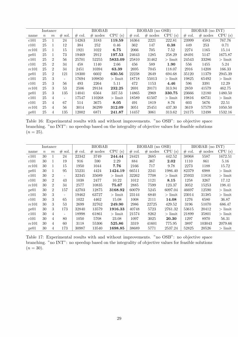
Instance BIOBAB BIOBAB (no OSB) BIOBAB (no INT)name n m # sol. # col. # nodes CPU (s) # col. # nodes CPU (s) # col. # nodes CPU (s)c101 25 1 24 14263 3183 119.59 16364 2221 222.81 23999 4583 767.76r101 25 1 12 384 252 0.46 362 147 0.38 449 253 0.71rc101 25 1 15 1921 1022 6.75 2066 705 7.52 2274 1165 15.14pr01 25 1 73 19469 2912 197.53 24643 1285 258.29 48491 5147 1675.87c101 25 2 56 25701 52255 5833.09 25810 31462 > limit 24543 33286 > limitr101 25 2 34 458 1140 2.66 456 589 1.90 556 1455 5.24rc101 25 2 34 2451 10394 63.39 2695 7045 118.07 2916 14208 166.33pr01 25 2 121 18300 6602 630.56 22238 2649 694.68 35120 11379 2945.39c101 25 3 - 17694 109850 > limit 18718 55013 > limit 19825 65492 > limitr101 25 3 56 493 2264 5.11 472 1153 4.46 596 3391 12.29rc101 25 3 53 2506 29134 232.25 2691 20171 313.94 2859 41579 462.75pr01 25 3 135 14041 6564 337.53 14865 2969 330.75 23666 12180 1480.50c101 25 4 - 17547 110268 > limit 18589 61507 > limit 19816 68731 > limitr101 25 4 67 514 3675 8.05 491 1819 8.76 603 5676 22.51rc101 25 4 56 3014 36299 312.09 3051 25451 437.30 3619 57579 1050.50pr01 25 4 135 12002 6871 241.87 14457 3061 313.62 24175 12498 1532.16

Table 16: Experimental results with and without improvements. ”no OSB”: no objective spacebranching. ”no INT”: no speedup based on the integrality of objective values for feasible solutions(n = 25).

Instance BIOBAB BIOBAB (no OSB) BIOBAB (no INT)name n m # sol. # col. # nodes CPU (s) # col. # nodes CPU (s) # col. # nodes CPU (s)c101 30 1 24 22342 3749 244.44 24421 2685 442.52 38968 5587 1672.51r101 30 1 19 916 590 2.29 884 367 2.02 1110 861 5.16rc101 30 1 15 1950 1044 7.76 2166 717 9.78 2273 1188 15.72pr01 30 1 95 55231 4424 1424.19 66511 2241 1986.40 82379 6988 > limitc101 30 2 - 32345 35689 > limit 32262 7708 > limit 25933 11816 > limitr101 30 2 43 1038 2477 10.22 1012 1121 8.15 1258 3267 17.12rc101 30 2 34 2577 10835 75.67 2885 7599 123.37 3052 15253 198.41pr01 30 2 157 42703 12875 3168.92 60079 5245 6097.04 46697 12590 > limitc101 30 3 - 19462 63727 > limit 23144 6840 > limit 23014 31385 > limitr101 30 3 65 1022 4462 15.08 1008 2111 14.08 1276 6580 36.87rc101 30 3 53 2699 32762 249.90 2986 22725 429.52 3196 51070 686.47pr01 30 3 173 32840 13579 1916.33 40748 5723 2761.32 53615 20412 > limitc101 30 4 - 18998 61861 > limit 21574 8262 > limit 21899 35801 > limitr101 30 4 80 1050 5708 23.08 1097 3025 20.30 1297 8970 56.31rc101 30 4 60 3118 55306 525.86 3319 41601 775.95 3897 103043 2079.66pr01 30 4 173 30987 13540 1698.85 38689 5771 2537.24 52825 20526 > limit

Table 17: Experimental results with and without improvements. ”no OSB”: no objective spacebranching. ”no INT”: no speedup based on the integrality of objective values for feasible solutions(n = 30).

29

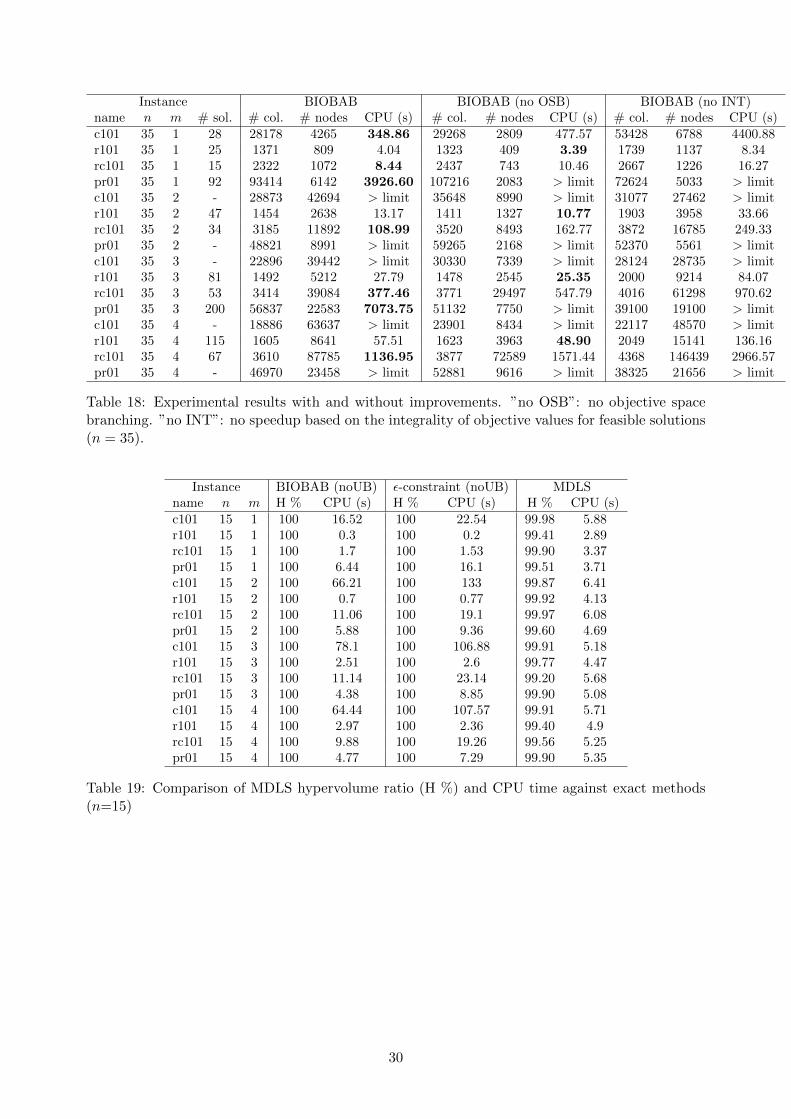
Instance BIOBAB BIOBAB (no OSB) BIOBAB (no INT)name n m # sol. # col. # nodes CPU (s) # col. # nodes CPU (s) # col. # nodes CPU (s)c101 35 1 28 28178 4265 348.86 29268 2809 477.57 53428 6788 4400.88r101 35 1 25 1371 809 4.04 1323 409 3.39 1739 1137 8.34rc101 35 1 15 2322 1072 8.44 2437 743 10.46 2667 1226 16.27pr01 35 1 92 93414 6142 3926.60 107216 2083 > limit 72624 5033 > limitc101 35 2 - 28873 42694 > limit 35648 8990 > limit 31077 27462 > limitr101 35 2 47 1454 2638 13.17 1411 1327 10.77 1903 3958 33.66rc101 35 2 34 3185 11892 108.99 3520 8493 162.77 3872 16785 249.33pr01 35 2 - 48821 8991 > limit 59265 2168 > limit 52370 5561 > limitc101 35 3 - 22896 39442 > limit 30330 7339 > limit 28124 28735 > limitr101 35 3 81 1492 5212 27.79 1478 2545 25.35 2000 9214 84.07rc101 35 3 53 3414 39084 377.46 3771 29497 547.79 4016 61298 970.62pr01 35 3 200 56837 22583 7073.75 51132 7750 > limit 39100 19100 > limitc101 35 4 - 18886 63637 > limit 23901 8434 > limit 22117 48570 > limitr101 35 4 115 1605 8641 57.51 1623 3963 48.90 2049 15141 136.16rc101 35 4 67 3610 87785 1136.95 3877 72589 1571.44 4368 146439 2966.57pr01 35 4 - 46970 23458 > limit 52881 9616 > limit 38325 21656 > limit

Table 18: Experimental results with and without improvements. ”no OSB”: no objective spacebranching. ”no INT”: no speedup based on the integrality of objective values for feasible solutions(n = 35).

Instance BIOBAB (noUB) ε-constraint (noUB) MDLSname n m H % CPU (s) H % CPU (s) H % CPU (s)c101 15 1 100 16.52 100 22.54 99.98 5.88r101 15 1 100 0.3 100 0.2 99.41 2.89rc101 15 1 100 1.7 100 1.53 99.90 3.37pr01 15 1 100 6.44 100 16.1 99.51 3.71c101 15 2 100 66.21 100 133 99.87 6.41r101 15 2 100 0.7 100 0.77 99.92 4.13rc101 15 2 100 11.06 100 19.1 99.97 6.08pr01 15 2 100 5.88 100 9.36 99.60 4.69c101 15 3 100 78.1 100 106.88 99.91 5.18r101 15 3 100 2.51 100 2.6 99.77 4.47rc101 15 3 100 11.14 100 23.14 99.20 5.68pr01 15 3 100 4.38 100 8.85 99.90 5.08c101 15 4 100 64.44 100 107.57 99.91 5.71r101 15 4 100 2.97 100 2.36 99.40 4.9rc101 15 4 100 9.88 100 19.26 99.56 5.25pr01 15 4 100 4.77 100 7.29 99.90 5.35

Table 19: Comparison of MDLS hypervolume ratio (H %) and CPU time against exact methods(n=15)

30

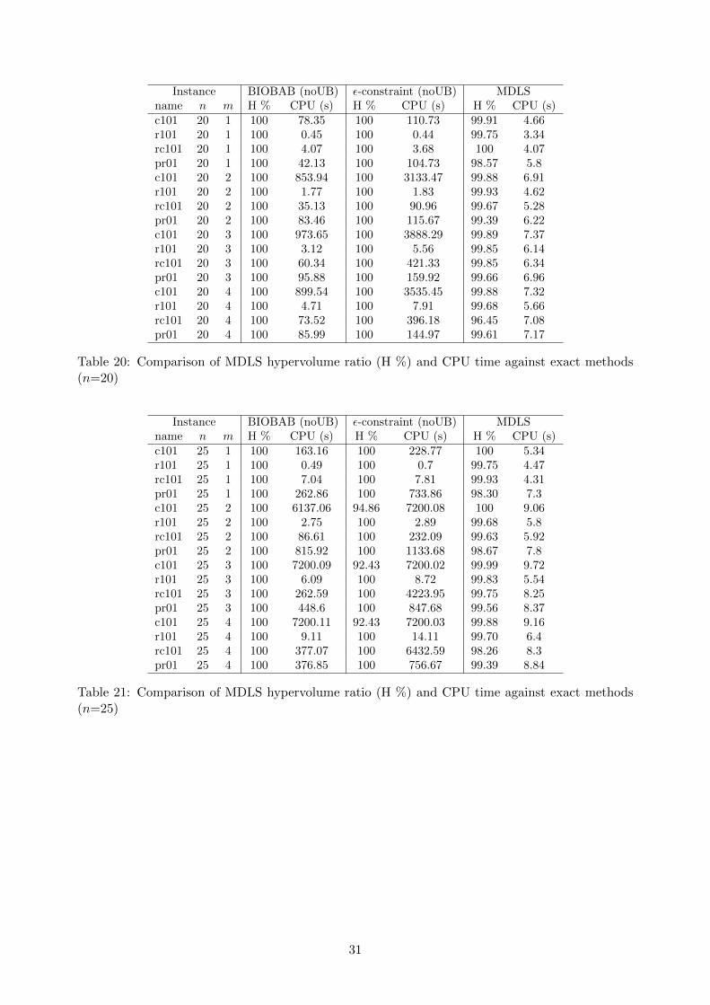
Instance BIOBAB (noUB) ε-constraint (noUB) MDLSname n m H % CPU (s) H % CPU (s) H % CPU (s)c101 20 1 100 78.35 100 110.73 99.91 4.66r101 20 1 100 0.45 100 0.44 99.75 3.34rc101 20 1 100 4.07 100 3.68 100 4.07pr01 20 1 100 42.13 100 104.73 98.57 5.8c101 20 2 100 853.94 100 3133.47 99.88 6.91r101 20 2 100 1.77 100 1.83 99.93 4.62rc101 20 2 100 35.13 100 90.96 99.67 5.28pr01 20 2 100 83.46 100 115.67 99.39 6.22c101 20 3 100 973.65 100 3888.29 99.89 7.37r101 20 3 100 3.12 100 5.56 99.85 6.14rc101 20 3 100 60.34 100 421.33 99.85 6.34pr01 20 3 100 95.88 100 159.92 99.66 6.96c101 20 4 100 899.54 100 3535.45 99.88 7.32r101 20 4 100 4.71 100 7.91 99.68 5.66rc101 20 4 100 73.52 100 396.18 96.45 7.08pr01 20 4 100 85.99 100 144.97 99.61 7.17

Table 20: Comparison of MDLS hypervolume ratio (H %) and CPU time against exact methods(n=20)

Instance BIOBAB (noUB) ε-constraint (noUB) MDLSname n m H % CPU (s) H % CPU (s) H % CPU (s)c101 25 1 100 163.16 100 228.77 100 5.34r101 25 1 100 0.49 100 0.7 99.75 4.47rc101 25 1 100 7.04 100 7.81 99.93 4.31pr01 25 1 100 262.86 100 733.86 98.30 7.3c101 25 2 100 6137.06 94.86 7200.08 100 9.06r101 25 2 100 2.75 100 2.89 99.68 5.8rc101 25 2 100 86.61 100 232.09 99.63 5.92pr01 25 2 100 815.92 100 1133.68 98.67 7.8c101 25 3 100 7200.09 92.43 7200.02 99.99 9.72r101 25 3 100 6.09 100 8.72 99.83 5.54rc101 25 3 100 262.59 100 4223.95 99.75 8.25pr01 25 3 100 448.6 100 847.68 99.56 8.37c101 25 4 100 7200.11 92.43 7200.03 99.88 9.16r101 25 4 100 9.11 100 14.11 99.70 6.4rc101 25 4 100 377.07 100 6432.59 98.26 8.3pr01 25 4 100 376.85 100 756.67 99.39 8.84

Table 21: Comparison of MDLS hypervolume ratio (H %) and CPU time against exact methods(n=25)

31

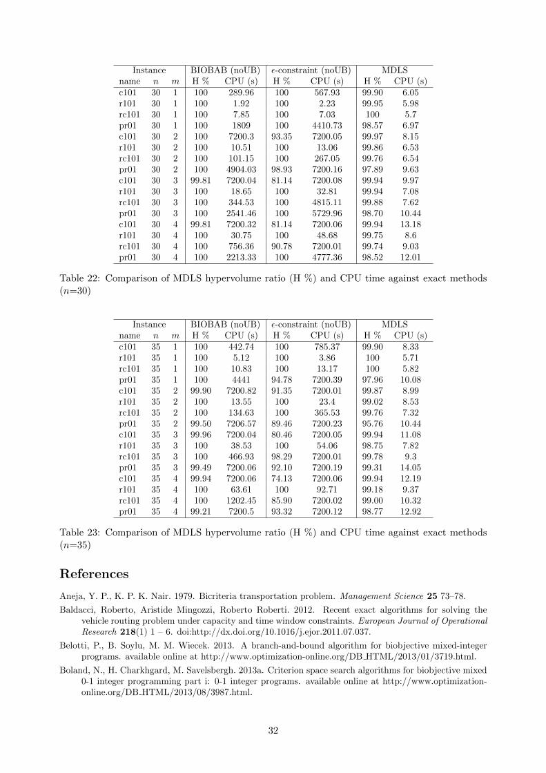
Instance BIOBAB (noUB) ε-constraint (noUB) MDLSname n m H % CPU (s) H % CPU (s) H % CPU (s)c101 30 1 100 289.96 100 567.93 99.90 6.05r101 30 1 100 1.92 100 2.23 99.95 5.98rc101 30 1 100 7.85 100 7.03 100 5.7pr01 30 1 100 1809 100 4410.73 98.57 6.97c101 30 2 100 7200.3 93.35 7200.05 99.97 8.15r101 30 2 100 10.51 100 13.06 99.86 6.53rc101 30 2 100 101.15 100 267.05 99.76 6.54pr01 30 2 100 4904.03 98.93 7200.16 97.89 9.63c101 30 3 99.81 7200.04 81.14 7200.08 99.94 9.97r101 30 3 100 18.65 100 32.81 99.94 7.08rc101 30 3 100 344.53 100 4815.11 99.88 7.62pr01 30 3 100 2541.46 100 5729.96 98.70 10.44c101 30 4 99.81 7200.32 81.14 7200.06 99.94 13.18r101 30 4 100 30.75 100 48.68 99.75 8.6rc101 30 4 100 756.36 90.78 7200.01 99.74 9.03pr01 30 4 100 2213.33 100 4777.36 98.52 12.01

Table 22: Comparison of MDLS hypervolume ratio (H %) and CPU time against exact methods(n=30)

Instance BIOBAB (noUB) ε-constraint (noUB) MDLSname n m H % CPU (s) H % CPU (s) H % CPU (s)c101 35 1 100 442.74 100 785.37 99.90 8.33r101 35 1 100 5.12 100 3.86 100 5.71rc101 35 1 100 10.83 100 13.17 100 5.82pr01 35 1 100 4441 94.78 7200.39 97.96 10.08c101 35 2 99.90 7200.82 91.35 7200.01 99.87 8.99r101 35 2 100 13.55 100 23.4 99.02 8.53rc101 35 2 100 134.63 100 365.53 99.76 7.32pr01 35 2 99.50 7206.57 89.46 7200.23 95.76 10.44c101 35 3 99.96 7200.04 80.46 7200.05 99.94 11.08r101 35 3 100 38.53 100 54.06 98.75 7.82rc101 35 3 100 466.93 98.29 7200.01 99.78 9.3pr01 35 3 99.49 7200.06 92.10 7200.19 99.31 14.05c101 35 4 99.94 7200.06 74.13 7200.06 99.94 12.19r101 35 4 100 63.61 100 92.71 99.18 9.37rc101 35 4 100 1202.45 85.90 7200.02 99.00 10.32pr01 35 4 99.21 7200.5 93.32 7200.12 98.77 12.92

Table 23: Comparison of MDLS hypervolume ratio (H %) and CPU time against exact methods(n=35)

References

Aneja, Y. P., K. P. K. Nair. 1979. Bicriteria transportation problem. Management Science 25 73–78.

Baldacci, Roberto, Aristide Mingozzi, Roberto Roberti. 2012. Recent exact algorithms for solving thevehicle routing problem under capacity and time window constraints. European Journal of OperationalResearch 218(1) 1 – 6. doi:http://dx.doi.org/10.1016/j.ejor.2011.07.037.

Belotti, P., B. Soylu, M. M. Wiecek. 2013. A branch-and-bound algorithm for biobjective mixed-integerprograms. available online at http://www.optimization-online.org/DB HTML/2013/01/3719.html.

Boland, N., H. Charkhgard, M. Savelsbergh. 2013a. Criterion space search algorithms for biobjective mixed0-1 integer programming part i: 0-1 integer programs. available online at http://www.optimization-online.org/DB HTML/2013/08/3987.html.

32

Boland, N., H. Charkhgard, M. Savelsbergh. 2013b. Criterion space search algorithms for biobjective mixed0-1 integer programming part II: Mixed integer programs. available online at http://www.optimization-online.org/DB FILE/2013/11/4107.pdf.

Chalmet, LG, L Lemonidis, DJ Elzinga. 1986. An algorithm for the bi-criterion integer programmingproblem. European Journal of Operational Research 25(2) 292–300.

Chao, I, Bruce L Golden, Edward A Wasil, et al. 1996. A fast and effective heuristic for the orienteeringproblem. European Journal of Operational Research 88(3) 475–489.

Cordeau, Jean-Francois, Michel Gendreau, Gilbert Laporte. 1997. A tabu search heuristic for periodic andmulti-depot vehicle routing problems. Networks 30(2) 105–119.

Dachert, K., J. Gorski, K. Klamroth. 2012. An augmented weighted tchebycheff method with adaptivelychosen parameters for discrete bicriteria optimization problems. Computers & Operations Research39 2929–2943.

Desrosiers, Jacques, Marco E Lubbecke. 2005. A primer in column generation. Guy Desaulniers, JacquesDesrosiers, Marius M. Solomon, eds., Column Generation. Springer US, 1–32.

Ehrgott, Matthias. 2005. Multicriteria optimization, vol. 2. Springer.

Ehrgott, Matthias, Xavier Gandibleux. 2006. Bound sets for biobjective combinatorial optimization prob-lems. Computers & Operations Research 34 2674–2694.

Feillet, Dominique, Pierre Dejax, Michel Gendreau, Cyrille Gueguen. 2004. An exact algorithm for theelementary shortest path problem with resource constraints: Application to some vehicle routingproblems. Networks 44(3) 216–229.

Geoffrion, Arthur M. 1968. Proper efficiency and the theory of vector maximization. Journal of MathematicalAnalysis and Applications 22 618–630.

Haimes, Y., L. Lasdon, D Wismer. 1971. On a bicriterion formulation of the problems of integrated systemidentification and system optimization. IEEE Transactions on systems, man and cybernetics 1 296–297.

Jozefowiez, N., G. Laporte, F. Semet. 2012. A generic branch-and-cut algorithm for multiobjective opti-mization problems: application to the multilabel traveling salesman problem. INFORMS Journal onComputing 24 554–564.

Laumanns, M., L. Thiele, E. Zitzler. 2006. An efficient, adaptive parameter variation scheme for meta-heuristics based on the epsilon-constraint method. European Journal of Operational Research 169932–942.

Leitner, M., I. Ljubic, M. Sinnl. 2014. The bi-objective prize-collecting steiner tree problem. INFORMSJournal on Computing to appear.

Masin, Michael, Yossi Bukchin. 2008. Diversity maximization approach for multiobjective optimization.Operations Research 56(2) 411–424. doi:10.1287/opre.1070.0413. URL http://pubsonline.informs.

org/doi/abs/10.1287/opre.1070.0413.

Mavrotas, G., D. Diakoulaki. 1998. A branch and bound algorithm for mixed zero-one multiple objectivelinear programming. European Journal of Operational Research 107 530–541.

Przybylski, Anthony, Xavier Gandibleux, Matthias Ehrgott. 2008. Two phase algorithms for the bi-objectiveassignment problem. European Journal of Operational Research 185(2) 509–533.

Raith, Andrea, Siamak Moradi, Matthias Ehrgott, Michael Stiglmayr. 2012. Exploring bi-objective columngeneration. Proceedings of the 46th Annual ORSNZ Conference. 288–296.

Righini, Giovanni, Matteo Salani. 2009. Decremental state space relaxation strategies and initializationheuristics for solving the orienteering problem with time windows with dynamic programming. Com-puters & Operations Research 36(4) 1191–1203.

Ropke, Stefan, David Pisinger. 2006. An adaptive large neighborhood search heuristic for the pickup anddelivery problem with time windows. Transportation Science 40(4) 455–472.

Sarpong, Boadu Mensah, Christian Artigues, Nicolas Jozefowiez. 2013. Column generation for bi-objectivevehicle routing problems with a min-max objective. 13th Workshop on Algorithmic Approaches forTransportation Modelling, Optimization, and Systems, ATMOS 2013, September 5, 2013, Sophia An-tipolis, France. 137–149.

Shaw, Paul. 1998. Using constraint programming and local search methods to solve vehicle routing problems.Principles and Practice of Constraint Programming – CP98 . Springer, 417–431.

33

Solomon, Marius M. 1987. Algorithms for the vehicle routing and scheduling problems with time windowconstraints. Operations research 35(2) 254–265.

Sourd, F., O. Spanjaard. 2008. A multi-objective branch-and-bound framework: application to the biobjec-tive spanning tree problem. INFORMS Journal on Computing 20 472–484.

Stidsen, T., K. A. Andersen, B. Dammann. 2014. A branch and bound algorithm for a class of biobjectivemixed integer programs. Management Science Available online.

Tam, Bassy, Matthias Ehrgott, David Ryan, Golbon Zakeri. 2011. A comparison of stochastic programmingand bi-objective optimisation approaches to robust airline crew scheduling. OR Spectrum 33(1) 49–75.doi:10.1007/s00291-009-0164-9. URL http://dx.doi.org/10.1007/s00291-009-0164-9.

Tricoire, Fabien. 2012. Multi-directional local search. Computers & Operations Research 39(12) 3089–3101.

Tuyttens, D., J. Teghem, P. H. fortemps, K. Van Nieuwenhuyze. 2000. Performance of the mosa methodfor the bicriteria assignment problem. Journal of Heuristics 6 295–310.

Ulungu, E.L., J. Teghem. 1995. The two phases method: An efficient procedure to solve bi-objectivecombinatorial optimization problems. Foundations of Computing and Decision Sciences 20(2) 149–165.

Vansteenwegen, Pieter, Wouter Souffriau, Greet Vanden Berghe, Dirk Van Oudheusden. 2009. Iteratedlocal search for the team orienteering problem with time windows. Computers & Operations Research36(12) 3281–3290.

Vincent, T., F. Seipp, S. Ruzika, A. Przybylski, X. Gandibleux. 2013. Multiple objective branch and boundfor mixed 0-1 linear programming: Corrections and improvements for the biobjective case. Computers& Operations Research 40 498–509.

Visee, M., J. Teghem, M. Pirlot, E. L. Ulungu. 1998. Two-phases method and branch and bound proceduresto solve the bi–objective knapsack problem. J. of Global Optimization 12(2) 139–155.

34