bounded distance decoding of linear error-correcting codes with gröbner bases

Journal of Symbolic Computation 44 (2009) 1626–1643

Contents lists available at ScienceDirect

Journal of Symbolic Computation

journal homepage: www.elsevier.com/locate/jsc

Bounded distance decoding of linear error-correcting codeswith Gröbner basesI

Stanislav Bulygin a,1, Ruud Pellikaan ba Department of Mathematics, University of Kaiserslautern, Room No. 48-437, P.O. Box 3049, 67653 Kaiserslautern, Germanyb Department of Mathematics and Computing Science, Eindhoven University of Technology, P.O. Box 513, NL-5600 MB, Eindhoven,The Netherlands

a r t i c l e i n f o

Article history:Received 4 October 2006Accepted 20 December 2007Available online 28 November 2008

Keywords:DecodingGröbner basisLinear codeMinimum distanceSyndrome decodingSystem of polynomial equations

a b s t r a c t

Theproblemof boundeddistance decoding of arbitrary linear codesusing Gröbner bases is addressed. A new method is proposed,which is based on reducing an initial decoding problem to solvinga certain system of polynomial equations over a finite field. Thepeculiarity of this system is that, when we want to decode up tohalf the minimum distance, it has a unique solution even overthe algebraic closure of the considered finite field, although fieldequations are not added. The equations in the system have degreeat most 2. As our experiments suggest, our method is much fasterthan the one of Fitzgerald–Lax. It is also shownvia experiments thatthe proposed approach in some range of parameters is superior tothe generic syndrome decoding.

© 2008 Elsevier Ltd. All rights reserved.

1. Introduction

In this paperwe consider bounded distance decoding of arbitrary linear codes using Gröbner bases.In recent years a lot of attention has been devoted to this question for cyclic codes which form aparticular subclass of linear codes. In this paper we consider a method for decoding arbitrary linearcodes. The reader is assumed to be familiar with the basics of error-correcting codes and Gröbnerbases theory. Introduction material can be taken for instance from Berlekamp (1968), Peterson andWeldon (1977), Cox et al. (1997) and Greuel and Pfister (2002), respectively.

I The first author was funded by ‘‘Cluster of Excellence in Rhineland-Palatinate’’.E-mail addresses: [email protected] (S. Bulygin), [email protected] (R. Pellikaan).URLs: http://www.mathematik.uni-kl.de/∼bulygin/ (S. Bulygin), http://www.win.tue.nl/∼ruudp/ (R. Pellikaan).

1 Tel.: +49 0631 205 2738; fax: +49 0631 205 4795.

0747-7171/$ – see front matter© 2008 Elsevier Ltd. All rights reserved.doi:10.1016/j.jsc.2007.12.003

http://www.elsevier.com/locate/jsc

http://www.elsevier.com/locate/jsc

mailto:[email protected]

mailto:[email protected]

http://www.mathematik.uni-kl.de/~bulygin/






http://www.win.tue.nl/~ruudp/






http://dx.doi.org/10.1016/j.jsc.2007.12.003

S. Bulygin, R. Pellikaan / Journal of Symbolic Computation 44 (2009) 1626–1643 1627

Quite a lot of methods exist for decoding cyclic codes and the literature on this topic is vast.We just mention Arimoto (1961), Berlekamp (1968), Gorenstein and Zierler (1961), Massey (1969),Peterson (1960), Peterson and Weldon (1977) and Sugiyama et al. (1975). All these methods are ofpolynomial complexity and efficient in practice, but do not correct up to the true error-correctingcapacity. Techniques using the theory of Gröbner baseswere addressed to remedy this problem. Thesemethods can be roughly divided into the following categories:

- Unknown syndromes: Berlekamp (1968, pp. 231–240), Tzeng et al. (1971), Hartmann (1972) andHartmann and Tzeng (1974);- Newton identities: Augot et al. (1990, 1992, 2007, 2002) and Chen et al. (1994c);- Power sums: Cooper (1990, 1991, 1993), Chen et al. (1994a,c,b), Loustaunau and York (1997),Carboara and Mora (2002) and Orsini and Sala (2005).

For arbitrary linear codes some generalizations are known, e.g. Fitzgerald (1996), Fitzgerald and Lax(1998), Borges-Quintana et al. (2006, 2005, 2007), Giorgetti and Sala (in press) and Orsini and Sala(2007). Our method is a generalization of the first one of unknown syndromes for arbitrary linearcodes.Finding a Gröbner bases has complexity that is doubly exponential in the number of variables, and

it is still exponential in the case of a finite number of solutions. Some experiments have been donebut it is difficult to estimate the complexity of the decoding algorithms that use Gröbner bases. Theexisting decoding algorithms of arbitrary linear codes all have complexities that are exponential inthe code length, see Barg (1998). The problem turns out to be even harder, as decoding algorithmsremain exponential even if one allows unbounded preprocessing, see Bruck and Naor (1990). So farno asymptotic results of decoding algorithms with Gröbner bases are known that are better than thecomplexity of the existing general decoding algorithms. We continued research in this direction inBulygin and Pelikkan (in preparation).

Notations: A field is denoted by F and its algebraic closure by F. The finite field with q elements isdenoted by Fq. If I is an ideal in the polynomial ring F[X1, . . . Xn] over F, then a zero or a solution of Iis a point x ∈ Fn such that f (x) = 0 for all f ∈ I . Variables are denoted by capital letters such as X, Yand U , and specific values by x, y and u, respectively. The vectors are denoted in bold, e.g. u, v. Thezero set of I is the set of all solutions of I in Fn and is denoted by Z(I). If I is an ideal in Fq[X1, . . . , Xn],then the set of solutions of I over Fq is denoted by Zq(I), and the ideal I + 〈X

qi − Xi, i = 1, . . . , n〉 is

denoted by Iq. So Zq(I) = Z(I) ∩ Fnq = Z(Iq).

2. Syndrome decoding with Gröbner bases

In this section we give a formulation of the well-known syndrome decoding in terms of ideals andsolutions of the corresponding systems.Moreover, some results of this section (e.g. Lemma 9) are laterused in Section 4, where we look closely on the structure of ideals that we need in our constructionfor decoding.Let C be a linear code over Fq of length n, dimension k and minimum distance d. The parameters

of C are denoted by [n, k, d] and its redundancy by r = n − k. The (true) error-correcting capacityb(d−1)/2c of the code is denoted by e. Choose a parity-checkmatrixH of C . Leth1, . . . ,hr be the rowsof H .

Remark 1. Let C = FqmC be the code over Fqm that is generated by C . Then C is the restriction of C toFnq , that is C = Fnq ∩ C . And H is also a parity-check matrix of C , since the rank of H does not changeunder the extension from Fq to Fqm . Furthermore C and C have the same minimum distance, sincethis is equal to the minimum number of dependent columns of H , and this does not change under anextension of scalars.

Definition 2. The (known) syndrome s(H, y) of a word y with respect to H is the column vectors(H, y) = HyT. It has entries si(H, y) = hi · y for i = 1, . . . , n − k. The abbreviations s(y) andsi(y) are used for s(H, y) and si(H, y), respectively.

1628 S. Bulygin, R. Pellikaan / Journal of Symbolic Computation 44 (2009) 1626–1643

Remark 3. Let y = c + e be a received word with c ∈ C the codeword that was sent and e the errorvector. Then hi · c = 0 for all i = 1, . . . , r . So the syndromes of y and e with respect to H are equaland known:

si(y) := hi · y = hi · e = si(e).

Let h′1, . . . ,h′n be the n columns of H . If furthermore the support of e is equal to {i1, . . . , it}, then

s(y) = s(e) = ei1h′

i1 + · · · + eith′

it .

Therefore, if the distance of a received word to the code is t , then the syndrome vector of the receivedword is a linear combination of t columns of H . By syndrome decoding we mean an algorithm thatfinds such a linear combination. One way to accomplish this is to go though all possible t-subsets of{1, . . . , n} and see by linear algebra whether a linear combination of the corresponding columns of Hgives the syndrome vector. The complexity is therefore O(

(nt

)(n− k)t2).

Finding the minimum distance is similar, since we take the syndrome equal to the zero vector, sowe try to find the smallest number of columns of H that are linearly dependent.

Definition 4. Let y ∈ Fnq and let d(y, C) be the distance of y to C . A nearest codeword of y to C is anelement c ∈ C such that d(y, c) = d(y, C). LetL(y, C) be the list of nearest codewords of y to C .

Proposition 5. Let C = FqmC. If y ∈ Fnq , then d(y, C) = d(y, C) andL(y, C) = L(y, C).

Proof. (1) Now d(y, C) ≥ d(y, C), since C ⊆ C . There are d(y, C) columns of H such that anFqm-linear combination of these columns is equal to s(H, y). But y and H have entries in Fq. Henced(y, C) ≤ d(y, C). Therefore equality holds.(2) NowL(y, C) ⊆ L(y, C) by (1). Conversely, let c ∈ L(y, C) and t = d(y, C). Let e = y− c. Let

I = {i1, . . . , it} be the support of e that is the set of nonzero coordinates of e. LetHI be the submatrix ofH consisting of the columns hi1 , . . . , hit . Let s = Hy

T. Then s is a linear combination of the columns ofHI . So HI and the extended matrix [HI |s] have the same rank. This rank is t , otherwise we would havea proper subset I ′ of I such that HI ′ and HI have the same rank. But this would give an e′ with supportI ′ of weight t ′ < t and He′T = s. This gives c′ ∈ C with y = c′ + e′. So d(y, C) ≤ t ′ < t , a contraction.Hence HI and the extended matrix [HI |s] have the same rank t . So HIxT = s has a unique solutionx = (ei1 , . . . , eit )with entries in Fq. Hence and c = y− e ∈ Fnq ∩ C = C . Therefore c ∈ L(y, C). �

Definition 6. Let hi(E) be the linear function in Fq[E1, . . . , En] defined by

hi(E) =n∑j=1

hijEj.

Let E(y) be the ideal in Fq[E1, . . . , En] generated by the elements hi(E)− si(y) for all i = 1, . . . , n− k.Let J(t, n) be the ideal in Fq[E1, . . . , En] defined by

J(t, n) =⋂

1≤j1<···<jn−t≤n

〈Ej1 , . . . , Ejn−t 〉.

Let E(t, y) be the ideal generated by E(y) and J(t, n).

Lemma 7. (1) e is a solution of E(y) if and only if y = c+ e for some positive integer m and c ∈ FqmC.(2) e is a solution of J(t, n) if and only ifwt(e) ≤ t.(3) Let t = d(y, C). Then E(w, y) has no solution for allw < t. And e is a solution of E(t, y) if and only ify = c+ e for some c ∈ C andwt(e) = t.

Proof. (1) If y = c+ e for some c ∈ FqmC , then e is a solution of E(y) by Remarks 1 and 3.Conversely, if e is a solution of E(y), then s(y) = s(e) and e ∈ Fnqm for some positive integer m. So

s(y− e) = 0. Hence c = y− e is a codeword of FqmC and y = c+ e.


(2) If wt(e) ≤ t , then the support of e is contained in {k1, . . . , kt} for some k. Let {j1, . . . , jn−t} bethe complement of this support. Then e is a solution of the ideal 〈Ej1 , . . . , Ejn−t 〉. So e is an element ofthe zero set Z(〈Ej1 , . . . , Ejn−t 〉). Hence e is an element of the zero set⋃

1≤j1<···<jn−t≤n

Z(〈Ej1 , . . . , Ejn−t 〉) = Z(

∩1≤j1<···<jn−t≤n

〈Ej1 , . . . , Ejn−t 〉)= Z(J(t, n)).

So e is a solution of J(t, n)The converse is proved similarly and is left to the reader.(3) Is a direct consequence of (1) and (2) and Proposition 5. �

Theorem 8. Let H be a parity-check matrix of the code C. Let y be a received word. Let t be the smallestpositive integer such that E(t, y) has a solution.(1) Then the solutions e of E(t, y) correspond one-to-one to c inL(y, C).(2) If e is a solution of E(t, y) such that wt(e) ≤ (d(C) − 1)/2, then wt(e) = t and e is the unique

solution.

Proof. (1) is a direct consequence of Lemma 7(3).(2) is a consequence of (1) and the well-known fact that y has a unique nearest codeword in case

d(y, C) ≤ (d− 1)/2. �

Lemma 9. Let

I(t, n) = 〈Ei1 · · · Eit+1 |1 ≤ i1 < · · · < it+1 ≤ n〉.

Then I(t, n) = J(t, n).

Proof. Let Ei1 · · · Eit+1 be a generator of the ideal I(t, n) and let j be an increasing (n− t)-tuple. Then{i1, . . . , it+1} and {j1, . . . , jn−t} are subsets of {1, . . . , n} consisting of t + 1 and n − t elements,respectively. Hence their intersection is not empty, that is ir = js for some r and s. Hence

Ei1 · · · Eit+1 ∈ 〈Ejs〉 ⊆ 〈Ej1 , . . . , Ejn−t 〉.

Hence it is proved that I(t, n) ⊆ J(t, n).Now consider J(t, n)/I(t, n). Let f be a polynomial in J(t, n). Modulo I(t, n)we may assume that

f =∑

i=(i1,...,it ),1≤i1<···<it≤n

fiEαi1i1· · · E

αitit .

with fi ∈ Fq andαi are nonnegative integers,which depend on i. For every iwith 1 ≤ i1 < · · · < it ≤ nthere exists exactly one j such that 1 ≤ j1 < · · · < jn−t ≤ n and {j1, . . . , jn−t} is the complement of{i1, . . . , it} in {1, . . . , n}. Now f ∈ J(t, n). So f ∈ 〈Ej1 , . . . , Ejn−t 〉. This is only possible if fi = 0 sincethe sets of variables {Ei1 , . . . , Eit } and {Ej1 , . . . , Ejn−t } are disjoint. So fi = 0 for every such i. Hencef = 0. Therefore J(t, n) ⊆ I(t, n). �

Remark 10. The ideal J(t, n) is generated by( nt+1

)monomials of degree t + 1, and thus E(t, y) is

generated by n− k linear functions and( nt+1

)monomials of degree t + 1.

Example 11. Wenowprovide a small example explaining Theorem8. Consider a one error-correctingHamming code with parameters [7, 4, 3] over F2. Let y = (1, 0, 1, 0, 1, 1, 1) be a received word. Leta parity-check matrix be

H =

(1 1 0 1 1 0 01 0 1 1 0 1 01 1 1 0 0 0 1

).

The ideal E(1, y) is generated by the linear polynomials E1+ E2+ E4+ E5, E1+ E3+ E4+ E6+ 1, E1+E2 + E3 + E7 + 1 and the binomials EiEj, 1 ≤ i < j ≤ 7. Now E(1, y) has (0, 0, 1, 0, 0, 0, 0) as theunique solution in the algebraic closure. Moreover, the same situation takes place when we considera code with the parity-check matrix H over F8. In particular, one does not need to add field equationsin order to avoid spurious solutions.


3. Matrix in MDS form

In this section we introduce the notions of an MDS basis and an unknown syndrome and thecorresponding matrix. We establish some properties of the matrix of unknown syndromes.Let b1, . . . , bn be a basis of Fn. Now B is the n× nmatrix with b1, . . . , bn as rows.

Definition 12. The (unknown) syndrome u(B, e) of a word e with respect to B is the column vectoru(B, e) = BeT. It has entries ui(B, e) = bi · e for i = 1, . . . , n.

Remark 13. The matrix B is invertible, since its rank is n. The syndrome u(B, e) determines the errorvector e uniquely, since

B−1u(B, e) = B−1BeT = eT.

So the idea is based on finding the unknown syndrome of an error vector with respect to some specificbasis B. Then finding the error vector is trivial.The abbreviations u(e) and ui(e) are used for u(B, e) and ui(B, e), respectively. We have a linear

automorphism β of Fn, defined by β(e) = eBT with inverse map γ . This induces an isomorphism ofrings

β∗ : F[U1, . . . ,Un] −→ F[E1, . . . , En],

defined by

β∗(Ui) =n∑j=1

bijEj

and its inverse γ ∗, defined by

γ ∗(Ei) =n∑j=1

cijUj,

where the cij are the entries of B−1.

Definition 14. Define the coordinatewise star product of two vectors x, y ∈ Fn by x ∗ y =(x1y1, . . . , xnyn). Then bi ∗ bj is a linear combination of the basis vectors b1, . . . , bn, that is thereare constants µijl ∈ F such that

bi ∗ bj =n∑l=1

µijl bl.

The elements µijl ∈ F are called the structure constants of the basis b1, . . . , bn. See Kostrikin andShafarevich (1990)

Definition 15. Define the n×nmatrix of (unknown) syndromesU(e) of aword e by uij(e) = (bi∗bj)·e.

Remark 16. The relation between the entries of the matrix U(e) and the vector u(e) of unknownsyndromes is given by

uij(e) =n∑l=1

µijl ul(e).

Proposition 17. The rank ofU(e) is equal to the weight of e.

Proof. See Høholdt et al. (1998, Lemma 4.7). See also Proposition 25. �

Remark 18. So there arewt(e)+1 columns ofU(e) that are dependent and everyw-tuple of columnsofU(e) is independent if w ≤ wt(e). We will look at the smallest t such that the first t + 1 columnsare dependent. For an arbitrary matrix B we have to go through all the w-tuples of columns ofU(e)withw ≤ wt(e)+1 to find such a dependency. This is not very efficient. There is a more efficient waywith the help of a B in special form.


Definition 19. Let b1, . . . , bn be a basis of Fn. Let Bs be the s × n matrix with b1, . . . , bs as rows, soB = Bn. We say that b1, . . . , bn is an orderedMDS basis and B anMDSmatrix if all the s× s submatricesof Bs have rank s for all s = 1, . . . , n. Let Cs be the code with Bs as parity-check matrix.

Remark 20. Let B be an MDS matrix. Then Cs is an MDS code for all s. This motivates the name in theprevious definition.

Definition 21. Let F = Fq. Suppose n ≤ q. Let x = (x1, . . . , xn) be an n-tuple of pairwise distinctelements in F. Define

bi = (xi−11 , . . . , xi−1n ).

Then b1, . . . , bn is called an ordered Vandermonde basis and the corresponding matrix is denoted byB(x) and called a Vandermonde matrix.In particular, if α ∈ F∗ is an element of order n and xj = αj−1 for all j, then b1, . . . , bn is called an

ordered Reed–Solomon (RS) basis and the corresponding matrix is called a RS matrix and denoted byB(α).

Remark 22. If b1, . . . , bn is a Vandermonde basis of Fn, then it is anMDS basis. Note that an RSmatrixis symmetric.For a finite field and general n there is a positive integerm such that n ≤ qm. The above construction

gives a Vandermonde basis b1, . . . , bn of Fnqm over Fqm such that

uij(e) = ui+j−1(e) if i+ j ≤ n+ 1.

In case n and q are relatively prime, then n divides qm − 1 for some m, and we can take an elementα ∈ F∗qm of order n and xj = α

j−1 for i = 1, . . . , n as for cyclic codes. In that case uij(e) = ui+j−1(e)for all i, jmodulo n.

Remark 23. Let C = FqmC be the code over Fqm that is generated by C . Then C is the restriction of Cto Fnq , that is C = Fnq ∩ C . Furthermore C and C have the same minimum distance by Remark 1.For any prime p and positive integer M there is an algorithm of polynomial computing time

(p logM)O(1) that computes an irreducible polynomial of degree m = M + o(M) over Fp. SeeShparlinski (1993, 1999). Hence for a given field Fq, the complexity of finding an extension Fqm suchthat qm ≥ n, is polynomial in n.Thus the code C can be efficiently realized for a given C .

Definition 24. LetM be a matrix with entrymij in row i and column j. ThenMv is the submatrix ofMconsisting of the first v columns, andMuv is the u× v submatrix ofM given by

Muv =

m11 m12 . . . m1vm21 m22 . . . m2v...

.... . .

...mu1 mu2 . . . muv

.Proposition 25. Suppose that B is an MDS matrix. Letw = wt(e). Then

rank(Unv(e)) = min{v,w}.

Proof. We have that

uij(e) = (bi ∗ bj) · e =n∑l=1

bilelbjl.

Hence

Unv(e) = BD(e)BTv,

where D(e) is the diagonal matrix with e on the diagonal. This triple product implies thatrank(Unv(e)) ≤ min{v,w}, since rank(B) = n, rank(Bv) = v and rank(D(e)) = w.


Wemay assume without loss of generality that the nonzero entries of e are at the beginning, sinceB stays an MDS matrix after a permutation of its columns. So the nonzero entries are e1, . . . , ew . Lete′ = (e1, . . . , ew). Then BD(e)BTv has BwD(e

′)BTvw as a submatrix. Now D(e′) is invertible, since all the

coordinates of e′ are nonzero. Hence BwD(e)BTv has the same rank as BwBTvw . Now Bww is invertible,

since B is an MDS matrix. Hence BwBTvw has the same rank as BTvw . But rank(Bvw) = min{v,w}, again

since B is MDS. Therefore rank(Unv(e)) ≥ min{v,w}. �

4. Determinantal variety of syndromes

In the previous section it is shown that Unv(e) has rank v if v ≤ wt(e), and its rank is wt(e) ifv > wt(e). We see that the first moment of stabilization of the rank of Unv(e) yields the weightof e. We would like to be able to find this moment. For this we change all the entries of Unv(e) tovariables and search for linear dependence of columns, see Definitions 26 and 39. The correspondingresults are developed in this section. It turns out that the study of the corresponding ideal also givesan opportunity to find a vector of unknown syndromes u.

Definition 26. Let B be an MDS matrix with structure constants µijl . Define the linear functions Uij inthe variables U1, . . . ,Un by

Uij =n∑l=1

µijl Ul.

LetU be the n× nmatrix with entries Uij.

Remark 27. If Ui = ui(e) for all i, then Uij = uij(e) for all i, j. So the matrix above exactly reflects theidea stated at the beginning of this section.

Definition 28. Let b′1, . . . , b′n be the columns of B. Let i = (i1, . . . , it)with 1 ≤ i1 < · · · < it ≤ n. Let

L(i) be the linear subspace of the vector space Fn generated by b′i1 , . . . , b′

it . That is

L(i) = {x1b′i1 + · · · + xtb′

it | x1, . . . , xt ∈ F}.

Let I(i) be the defining ideal of L(i) in F[U1, . . . ,Un]. That is

I(i) = {f (U) ∈ F[U1, . . . ,Un] | f (u) = 0 for all u ∈ L(i)}.

Lemma 29. Letk be a t-tuple of increasing entries and let {j1, . . . , jn−t} be the complement of {k1, . . . , kt}in {1, . . . , n}. Then L(k) has dimension t and the ideal I(k) is a radical ideal generated by the n− t linearfunctions γ ∗(Ej1), . . . , γ

∗(Ejn−t ) in the variables U1, . . . ,Un.

Proof. The dimension of L(k) follows formDefinition 28 and the fact that b′1, . . . , b′n are independent.

Now u = u(e) = BeT = e1b′1 + · · · + enb′n. Furthermore wt(e) ≤ t if and only if the support

of e is contained in {k1, . . . , kt} for some k with 1 ≤ k1 < · · · < kt ≤ n. Let β and γ be themaps of Remark 13. Then u ∈ I(k) if and only if e = γ (u) and ej1 = · · · = ejn−t = 0. Soβ∗(I(k)) = 〈Ej1 , . . . , Ejn−t 〉 is a radical ideal. Hence the ideal I(k) is also radical and generated by then − t linear functions γ ∗(Ej1), . . . , γ

∗(Ejn−t ) in the variables U1, . . . ,Un, since β∗ is an isomorphism

with inverse γ ∗. �

Remark 30. If i = (i1, . . . , it), j = (j1, . . . , iu) and k = (k1, . . . , kv) consist of increasing entries suchthat {i1, . . . , it} ∩ {j1, . . . , iu} = {k1, . . . , kv}, then L(i) ∩ L(j) = L(k). This fact is left to the reader tocheck.

Definition 31. LetV be an l×mmatrixwith entries inF[U1, . . . ,Un]. Let I(t,V)be the ideal generatedby the determinants of all (t+ 1)× (t+ 1) submatrices ofVl,t+1. Let Z(t,V) be the zero set of I(t,V)in Fn.

Remark 32. The ideal I(t,V) is invariant under elementary row operations and elementary columnoperations on the first t + 1 columns. In particular I(t,V) = I(t, SV) if V is an l×mmatrix and S isan invertible l× lmatrix. See Bruns and Vetter (1988).


Remark 33. Let u ∈ Fn. The rank of Vl,t+1 at u is at most t if and only if u ∈ Z(t,V). See Bruns andVetter (1988).

Theorem 34. The variety Z(t,U) is the union of the(nt

)irreducible components L(k) with 1 ≤ k1 <

· · · < kt ≤ n. Furthermore I(t,U) is a radical ideal with

I(t,U) =⋂

1≤k1<···<kt≤n

I(k).

Proof. Let u ∈ Fn and Ui = ui for all i. Then u = u(e) for some e ∈ Fn by Remark 13. HenceUij = uij(e) by Remark 27. Now u ∈ Z(t,U) if and only if rank(Un,t+1(e)) ≤ t . But rank(Un,t+1(e))is equal to min{t + 1,wt(e)} by Proposition 25. Hence u ∈ Z(t,U) if and only if wt(e) ≤ t . Nowu = u(e) = BeT = e1b′1 + · · · + enb

′n. Furthermore wt(e) ≤ t if and only if the support of e is

contained in {k1, . . . , kt} for some k with 1 ≤ k1 < · · · < kt ≤ n. Therefore u ∈ Z(t,U) if andonly if u ∈ L(k) for some t-tuple k with increasing entries by Lemma 29. Note that a linear space isirreducible. Hence Z(t,U) is the union of the

(nt

)irreducible components L(k).

Let D(E) be the diagonal matrix with the variables E1, . . . , En on the diagonal. Then thecomponentwise application of β∗ to the entries ofU yields

β∗(U) = BD(E)BT,

because

β∗(Uij) = β∗(

n∑l=1

µijl Ul

)=

n∑l=1

n∑l′=1

µijl bll′El′ =

n∑l′=1

bil′bjl′El′ ,

since bi ∗ bj =∑nl=1 µ

ijl bl.

Remark 32 yields

I(t,U) = I(t,Un,t+1) = I(t, B−1Un,t+1).

Now β∗(Un,t+1) = BD(E)BTt+1. So β∗(B−1Un,t+1) = D(E)BTt+1. Let i be an (t + 1)-tuple with

1 ≤ i1 < · · · < it+1 ≤ n. Then the (t + 1) × (t + 1)minor of β∗(B−1Un,t+1) consisting of the rowsindexed by i is up to a nonzero scalar equal to Ei1 · · · Eit+1 , since all the (t + 1)× (t + 1) submatricesof Bt+1 have rank t + 1. Therefore β∗(I(t,U)) is generated by all (t + 1)-fold products Ei1 · · · Eit+1 . So

β∗(I(t,U)) =⋂

1≤j1<···<jn−t≤n

〈Ej1 , . . . , Ejn−t 〉

by Lemma 9. The inverse of the map β∗ is γ ∗ by Remark 13. Hence

I(t,U) =⋂

1≤j1<···<jn−t≤n

〈γ ∗(Ej1), . . . , γ∗(Ejn−t )〉 =

⋂1≤k1<···<kt≤n

I(k)

by Lemma 29. Therefore I(t,U) is radical, since it is an intersection of radical ideals. �

Remark 35. The ideal I(t,U) is equal to γ ∗(I(t, n)) and is generated by( nt+1

)homogeneous

polynomials of degree t + 1. See also Lemma 9 and Remark 10.

Remark 36. (1) For definitions and properties of determinantal ideals, rings and varieties we referto the early work of Room (1938) and the more recent books (Bruns and Vetter, 1988; Eisenbud,1995). Determinantal rings are Cohen–Macaulay by Eagon andHochster, see Eisenbud (1995, Theorem18.18). Consequently determinantal ideals are unmixed (Eisenbud, 1995, Corollary 18.14), that is allassociated primes are minimal and have the same codimension, in particular there are no embeddedprimes (Eisenbud, 1995, Section 3.1).(2) In the case of Theorem 34 the ideal I(t,U) is generated by the t + 1 minors of a the n× (t + 1)

matrix Un,t+1 Hence the codimension of its zero set Z(t,U) is at most n − (t + 1) − 1. But allcomponents of Z(t,U) have in fact codimension n − t . Hence I(t,U) is a determinantal ideal andtherefore Cohen–Macaulay and unmixed. The associated primes of I(t,U) are minimal and have thesame codimension n− t . The minimal primes are the ideals I(k).


(3) The (t+1)× (t+1)minors of a generic matrixm×nmatrix X form a reduced Gröbner basis ofthe ideal generated by these minors, with respect to a certain lexicographic term order. See Sturmfels(1990). We think that a similar statement holds for I(t,U) and leave this as an open question.(4) The case that the matrixU is ‘‘Hankel’’, ‘‘Toeplitz’’ or ‘‘Catalecticant’’, that is where the entries

ofU are constant along diagonals: Uij = Ui+j−1, is treated in Eisenbud (1988).

Proposition 37. If t < n, then the singular locus of Z(t,U) is Z(t − 1,U).

Proof. For the notion of singular and regular point we refer to Eisenbud (1995, Section 16.6). Everycomponent L(i) of Z(t,U) is nonsingular, since it is a linear subspace. Hence the singular locus ofZ(t,U) is the union of all the intersections of two distinct components. If i = (i1, . . . , it) andj = (j1, . . . , it) consist of increasing entries, such that {i1, . . . , it} ∩ {j1, . . . , it} = {k1, . . . , kv} withk = (k1, . . . , kv), then L(i) ∩ L(j) = L(k) by Remark 30. If moreover i 6= j, then v ≤ t − 1 andL(i) ∩ L(j) ⊆ Z(t − 1,U).Conversely, let L(k) be a component of Z(t − 1,U) with k = (k1, . . . , kt−1). Then {i1, . . . , it} ∩

{j1, . . . , it} = {k1, . . . , kt−1} for some i = (i1, . . . , it) and j = (j1, . . . , it), since t < n. HenceL(k) = L(i) ∩ L(j) is in the singular locus of Z(t,U). �

Example 38. Let α be an element of F∗4 of order 3. Let B be the RS matrix with rows b1 = (1, 1, 1),b2 = (1, α, α2) and b3 = (1, α2, α). The matrixU is of the form (cf. Remark 22)(U1 U2 U3

U2 U3 U1U3 U1 U2

).

If t = 0, then Z(0,U) consists of the origin and indeed

I(0,U) = 〈U1,U2,U3〉.

For t = 1 we have that Z(1,U) is the union of the lines L(1), L(2) and L(3) through the origin withdirections b′1, b

′

2 and b′

3, respectively, given by the columns of B. And

I(1,U) = 〈U22 − U1U3,U21 − U2U3,U

23 − U1U2〉.

In case t = 2 we have that Z(2,U) is the union of the planes L(1, 2), L(1, 3) and L(2, 3), whereL(i, j) is the plane through the origin generated by b′i and b′j . The corresponding ideals are I(1, 2) =〈U1+αU2+α2U3〉, I(1, 3) = 〈U1+α2U2+αU3〉 and I(2, 3) = 〈U1+U2+U3〉, respectively. Furthermore

I(2,U) = 〈U31 + U32 + U

33 + U1U2U3〉.

Indeed we have that

I(2,U) = I(1, 2) ∩ I(1, 3) ∩ I(2, 3),

since

U31 + U32 + U

33 + U1U2U3 = (U1 + αU2 + α

2U3)(U1 + α2U2 + αU3)(U1 + U2 + U3).

Definition 39. The ideal I(t,U, V ) in the ringFq[U1, . . . ,Un, V1, . . . , Vt ] is generated by the elements

t∑j=1

UijVj − Uit+1 for i = 1, . . . , n.

Let Z(t,U, V ) be the zero set of I(t,U, V ) over Fq.

Remark 40. For every u there is a unique e such that u = u(e) by Remark 13. By evaluatingU at u(e)we see that (u, v) is an element of Z(t,U, V )) for some v if and only if the (t + 1)th column ofU(e)is a linear combination of the first t columns ofU(e).

Lemma 41. Let u = u(e). If u ∈ Z(t,U), then there is a t ′ ≤ t and a v such that (u, v) ∈ Z(t ′,U, V ).


Proof. Suppose u ∈ Z(t,U). Then rank(Un,t+1(e)) ≤ t by Remark 33. So the first t + 1 columns ofU(e) are linearly dependent. Hence there is a t ′ ≤ t such that the (t ′+1)th column ofU(e) is a linearcombination of the first t ′ columns ofU(e). Therefore (u, v) is an element of Z(t ′,U, V ) for some v,by Remark 40. �

Proposition 42.

I(t,U) ⊆ I(t,U, V ).

Proof. Let Rt be the factor ring F[U1, . . . ,Un, V1, . . . , Vt ]/I(t,U, V ). Then the following equationshold in the ring Rt

t∑l=1

UilVl − Uit+1 = 0 for all i = 1, . . . , n.

Let∆l be the determinant of the t × t submatrix ofUt,t+1 obtained by deleting the lth column. Then

∆t+1Vl = (−1)t+l∆l for all l = 1, . . . , t,

by Cramer’s rule, which holds in this form for a system of linear equations with entries in anycommutative ring with unit element (Lang, 1993, XIII, Section 4). Now det(Ut+1,t+1) is a generatingelement of I(t,U) and the cofactor expansion this determinant along the last row is

det(Ut+1,t+1) =

t∑l=1

Ut+1,l(−1)t+1+l∆l + Ut+1,t+1∆t+1

which is equal tot∑l=1

−Ut+1,l∆t+1Vl + Ut+1,t+1∆t+1 = −∆t+1

(t∑l=1

Ut+1,lVl − Ut+1,t+1

)= 0

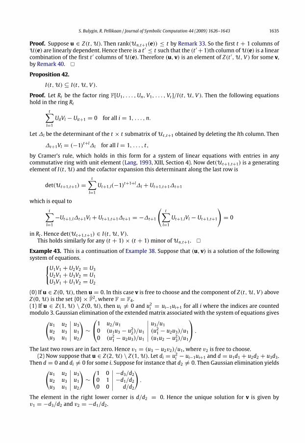
in Rt . Hence det(Ut+1,t+1) ∈ I(t,U, V ).This holds similarly for any (t + 1)× (t + 1)minor ofUn,t+1. �

Example 43. This is a continuation of Example 38. Suppose that (u, v) is a solution of the followingsystem of equations.{U1V1 + U2V2 = U3

U2V1 + U3V2 = U1U3V1 + U1V2 = U2

(0) If u ∈ Z(0,U), then u = 0. In this case v is free to choose and the component of Z(t,U, V ) aboveZ(0,U) is the set {0} × F2, where F = F4.(1) If u ∈ Z(1,U) \ Z(0,U), then ui 6= 0 and u2i = ui−1ui+1 for all i where the indices are countedmodulo 3. Gaussian elimination of the extendedmatrix associated with the system of equations gives(u1 u2 u3

u2 u3 u1u3 u1 u2

)∼

1 u2/u1 u3/u10 (u1u3 − u22)/u1 (u21 − u2u3)/u10 (u21 − u2u3)/u1 (u1u2 − u23)/u1

.The last two rows are in fact zero. Hence v1 = (u3 − u2v2)/u1, where v2 is free to choose.(2) Now suppose that u ∈ Z(2,U) \ Z(1,U). Let di = u2i − ui−1ui+1 and d = u1d1 + u2d2 + u3d3.

Then d = 0 and di 6= 0 for some i. Suppose for instance that d2 6= 0. Then Gaussian elimination yields(u1 u2 u3u2 u3 u1u3 u1 u2

)∼

(1 0 −d3/d20 1 −d1/d20 0 d/d2

).

The element in the right lower corner is d/d2 = 0. Hence the unique solution for v is given byv1 = −d3/d2 and v2 = −d1/d2.


5. Decoding up to half the minimum distance

Without loss of generality we may assume, after a finite extension of the finite field Fq, that n ≤ q.Let b1, . . . , bn be a basis of Fnq . From now on we assume that the corresponding matrix B is an MDSmatrix.Let C be an Fq-linear code with parameters [n, k, d]. Choose an r × n parity-check matrix H of

C with r = n − k. The row hi of H is a linear combination of the basis b1, . . . , bn, that is there areconstants aij ∈ Fq such that

hi =n∑j=1

aijbj.

In other words H = ABwhere A is the r × nmatrix with entries aij.

Remark 44. Let y = c + e be a received word with c ∈ C a codeword and e an error vector. Thesyndromes of y and e with respect to H are equal and known as noted in Remark 3 and they can beexpressed in the unknown syndromes of ewith respect to B:

si(y) = si(e) =n∑j=1

aijuj(e),

since hi =∑nj=1 aijbj and bj · e = uj(e).

Definition 45. The ideal J(y) in the ring Fq[U1, . . . ,Un] is generated by the elements

n∑l=1

ajlUl − sj(y) for j = 1, . . . , r.

Let J(t, y) be the ideal in Fq[U1, . . . ,Un, V1, . . . , Vt ] generated by J(y) and I(t,U, V ) fromDefinition 39.

Remark 46. The ideal J(t, y) is generated by n − k linear functions and n quadratic polynomials. Inprinciple, we can also express some n − k variables, say Uk+1, . . . ,Un, via k others, say U1, . . . ,Uk,using the parity-check matrix H , and then substitute in the quadratic part. In this way we obtain anideal generated by n quadratic polynomials in k+ t variables.

Lemma 47. If y = c+ e for some c ∈ C andwt(e) = t, then there is a v such that (u(e), v) is a solutionof J(t, y).

Proof. Let y = c + e for some c ∈ C and u = u(e). Then u is a solution of J(y) by Remark 44. If weevaluateU at u(e)we see that rank(Unv(e)) = min{v,wt(e)} by Proposition 25. Let wt(e) = t . Thenrank(Unv) = v if v < t and rank(Unv) = t if v ≥ t . So the (t + 1)th column of Un,t+1 is a linearcombination of the first t columns ofU. Hence there is a v such that (u, v) is a solution of I(t,U, V ),by Remark 40. Hence (u, v) is a solution of J(t, y). �

Lemma 48. Let (u, v) be a solution of J(t, y). Then there is a unique e of weight at most t such thatu = u(e), furthermore y = c+ e for some c in FqmC.

Proof. Let (u, v) be a solution of J(t, y). Then there is a unique e such that u = u(e) by Remark 13.The element u in Fnqm is a solution of J(y). Hence si(y) =

∑nj=1 aijuj(e) for all i. But si(e) =∑n

j=1 aijuj(e) for all i, and u = u(e). So s(y− e) = 0. Hence there is a c in FqmC such that y = c+ e.Now (u, v) is a solution of I(t,U, V ). Hence the (t + 1)th column ofU(e) is a linear combination

of the first t columns ofU(e), by Remark 40. Therefore rank(Un,t+1(e)) ≤ t . But rank(Un,t+1(e)) =min{t + 1,wt(e)} by Proposition 25. Hence wt(e) ≤ t . �


Lemma 49. If (u, v) and (u,w) are distinct solutions of J(t, y), then there is a solution (u, z) of J(t ′, y)for some t ′ with t ′ < t. If furthermore t ′ = 0, then y in FqmC for some m.

Proof. Let (u, v) and (u,w) be distinct solutions of J(t, y). Then u is a solution of J(y) and (u, v) and(u,w) are solutions of I(t,U, V ). There is a unique e such that u = u(e). Hence

t∑j=1

uijvj = ui,t+1 andt∑j=1

uijwj = ui,t+1 for all i.

Sot∑j=1

uij(vj − wj) = 0 for all i,

and v − w 6= 0, since v 6= w. Hence the first t columns of the matrix U(e) are linearly dependent.Therefore there is a t ′ < t such that column t ′ + 1 is a linear combination of the first t ′ columns. Inother words there is a solution (u, z) of J(t ′, y) by Remark 40.If t ′ = 0, then u = u(e) for a unique e and y = c + e for some c in FqmC and wt(e) ≤ 0, by

Lemma 48. Hence y in FqmC for somem. �

Theorem 50. Let B be an MDS matrix with structure constants µijl and linear functions Uij. Let H be aparity-check matrix of the code C. Let A be the matrix such that H = AB. Let y = c + e be a receivedword with c ∈ C the codeword sent and e the error vector. Suppose that wt(e) is not zero and at most(d(C) − 1)/2. Let t be the smallest positive integer such that J(t, y) has a solution (u, v) over Fq. Thenwt(e) = t and the solution is unique satisfying u = u(e).

Proof. (1) There is a solution (u(e), v) of J(wt(e), y) by Lemma 47.(2) Suppose that t is the smallest positive integer such that J(t, y) has a solution over Fq. Then

t ≤ wt(e) by (1).Suppose that (u, v) is a solution. Then there is a unique e ∈ Fnqm for somem such that u = u(e). Let

C = FqmC . Then y = c+e for some c ∈ C andwt(e) ≤ t by Lemma48. Now s(e) = s(y) = s(e). Hencee− e is a codeword of C . Now C and C have the sameminimum distance by Remark 1. By assumptionwe have that wt(e) ≤ (d(C) − 1)/2. The minimality of t implies wt(e) ≤ t ≤ wt(e). Hence e − e isa codeword C of weight strictly smaller than d(C). So e = e. Therefore, for every solution (u, v) wehave u = u(e). Thus we have proved that the u-part is unique.Now suppose that (u, v) and (u,w) are distinct solutions of J(t, y). Then there is a solution (u, z)

of J(t ′, y) for some 1 ≤ t ′ < t by Lemma 49, since y is not a codeword. This contradicts theminimalityof t . Hence the solution is unique. �

Theorem 51. Let y = c + e be a received word with c ∈ C the codeword sent and e the error vector.Suppose that wt(e) is not zero and at most (d(C) − 1)/2. Let t be the smallest positive integer such thatJ(t, y) has a solution. Then the solution is unique and the reduced Gröbner basis G for the ideal J(t, y)withrespect to any monomial ordering is

Ui − ui(e), i = 1, . . . , n,Vj − vj, j = 1, . . . , t,

where (u(e), v) is the unique solution.

Proof. There is a unique solution (u, v) with u = u(e) and wt(e) = t , by Theorem 50. So (u, v) ∈Z(t,U, V ). Hence u ∈ Z(t,U) by Proposition 42. So there is a k with 1 ≤ k1 < · · · < kt ≤ n suchthat u ∈ L(k) by Theorem 34. If there is another such k′ with u ∈ L(k′), then u ∈ Z(t − 1,U), byProposition 37. Hence there is a t ′ < t and a v′ such that (u, v′) ∈ Z(t ′,U, V ), by Lemma 41. But thiscontradicts the minimality of t . So u is not an element of Z(t − 1,U) and the k is unique. Hence

L(k) ∩ Z(J(y)) = {u}.


In otherwords Z(J(y)) is a linear affine space, Z(t,U) is a union of linear spaces, and Z(J(y)) intersectsexactly one of the components of Z(t,U). The intersection of these linear spaces is transversal, sincethe intersection consists of exactly one point. Hence J(y) + I(t,U) is equal to the maximal ideal〈U1 − u1, . . . ,Un − un〉. The Vj satisfy linear equations in the Uij which after evaluation at uij becomeconstants. The solution for the Vj is unique and equal to vj. Gaussian elimination gives that Vj − vj isan element of J(t, y). �

Remark 52. We note that in Augot et al. (2007) the authors also prove the uniqueness result forcyclic codes. Still they did not succeed in proving that their unique solution has multiplicity one. OurTheorem 51 states exactly this for arbitrary linear codes.

So we have that the system J(t, y), for t = wt(e), has a unique simple solution (u, v). It isknown from Theorem 50 that, u = u(e), the unknown syndrome of e, which lies in Fnq . But thenvia substitution of u to the system J(t, y) it is not hard to see that v is also from Fnq .We are now ready to formulate the algorithm for decoding. In the algorithm it is assumed that the

number of errors occurred does not exceed the error-correcting capacity of the code as in Theorems 50and 51.

Algorithm 53. We proceed as follows.

(1) Set i = 1.(2) Find the reducedGröbner basisGof the ideal J(i, y)with respect to anyordering chosen in advance.(3) If G = {1}, then i := i+ 1 and go to (2).(4) G is of the form {Uj−uj, Vl−vl}1≤j≤n,1≤l≤i. Form a vector u = (u1, . . . , un) of unknown syndromesof y.

(5) Compute eT = B−1u.(6) Return c := y− e.

Example 54. Consider the ternary Golay code of length 11 and dimension 6. The code is cyclic withdefining set {1} and complete defining set {1, 3, 4, 5, 9}. So the BCH bound implies that the minimumdistance is at least 4, but it is in fact 5. So the code is 2 error-correcting. But the decoding algorithmsby Peterson and Berlekamp–Massey correct only 1 error. Now m = 5 is the smallest degree of anextension such that F∗3m has an element α of order 11. The corresponding RS matrix is given by B =(α(i−1)(j−1)|1 ≤ i, j ≤ 11). Let H be the parity-check matrix over F243 that consists of the rows bi for iin the complete defining set. The matrix of syndromesU has entries Uij = Ui+j−1, where the indicesi, j are takenmodulo n. For a received word ywe have that the syndromes si = y(αi) =

∑11j=1 yjα

i(j−1)

for i = 1, 3, 4, 5, 9 are known. Hence the ideal J(y) is generated by the elements Ui − si, for i inthe complete defining set. If there are no errors, then s1 = 0. If there is one error, then s221 = 1Now suppose that the received word has 2 errors. Then s2421 = 1 and s221 6= 1. The quadraticequations

2∑j=1

Ui+j−1Vj = Ui+2 for i = 1, . . . , n

from J(t, y) become for i = 3, 4{s3V1 + s4V2 = s5s4V1 + s5V2 = U6.

Now s3 = s31, s4 = s811 and s5 = s

271 . Hence ∆ = s3s5 − s

24 = s

301 (1 − s

1321 ) 6= 0. So V1 and V2 can be

expressed as linear functions in U6.{V1 = (s25 − s4U6)/∆V2 = (s3U6 − s4s5)/∆.


The remaining equations give that Ui is a polynomial in U6 of degree i− 5 for i > 6. In fact the Ui, V1and V2 are polynomials in s1. See Higgs and Humphreys (1993).

Remark 55. In the cryptosystem of McEliece (1978) or Niederreiter (1986) a generator matrix orparity-check matrix is scrambled by permuting the coordinate positions and is used as the publickey. For instance let H1 be a ternary parity-check matrix of the ternary Golay code. Let S be aninvertible 5 × 11 matrix and P a 11 × 11 permutation matrix. Then H2 = SH1P is the public key.It is assumed that H2 looks like a random chosen matrix for an eavesdropper. Only those decodingalgorithms can be used for his attack that have arbitrary codes as input. If our method would be used,then B2 is an 11 × 11 MDS matrix over F27 since this is the smallest extension of F3 for which sucha matrix exists. The parity-check matrix H2 and the matrix B2 do not match so nicely anymore. Wecould use the linear equations in J(y) to eliminate 5 variables. Than we are left with 11 quadraticequations in the 8 variables U1, . . . ,U6 and V1, V2, and in general there are no linear equations amongthem.

6. Simulations and experimental results

All computations in this section are undertaken on AMD Opteron Processor 242 (1.6 MHz), 8 GBRAM under Linux. The computations of Gröbner bases are realized in SINGULAR 3-0-3 (Greuel et al.,2007). The command used is std.

6.1. Random binary codes

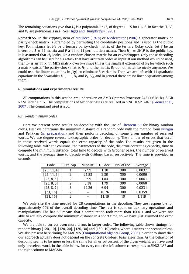
Here we present some results on decoding with the use of Theorem 50 for binary randomcodes. First we determine the minimum distance of a random code with the method from Bulyginand Pelikkan (in preparation) and then perform decoding of some given number of receivedwords. We use degree reverse lexicographic order for decoding. The number of errors that occurin these received words equals the error capacity of the code. The results are given in thefollowing table, with the columns: the parameters of the code, the error-correcting capacity, time tocompute the minimum distance, total time to decode with Gröbner bases, the number of receivedwords, and the average time to decode with Gröbner bases, respectively. The time is provided inseconds.

Code Err. cap. Mindist. GB dec. No. of rec. Average[25, 11, 4] 1 2.99 1.10 300 0.0037[25, 11, 5] 2 21.58 2.89 300 0.0096[25, 8, 5] 2 0.99 1.84 300 0.0061[25, 8, 6] 2 3.38 1.79 300 0.0060[25, 8, 7] 3 12.26 6.94 300 0.0231[31, 15] 2 – 10.76 300 0.0359[31, 15] 3 – 11.19 10 1.119

We only cite the time needed for GB computations in the decoding. They are responsible forapproximately 90% of the overall decoding time. The rest is spent on auxiliary operations andmanipulations. The bar ‘‘-’’ means that a computation took more than 1000 s. and we were notable to actually compute the minimum distance in a short time, so we have just assumed the errorcapacity.We are able to correct even more errors in larger codes. The following table shows timings for

random binary [120, 10], [120, 20], [120, 30] and [150, 10] codes, where 1means one second or less.We also present here timing for MAGMA (Computational Algebra Group, 2005) in order to show thatour approach actually does not depend on the concrete Gröbner basis algorithm. As the behavior ofdecoding seems to be more or less the same for all error-vectors of the given weight, we have usedonly 1 received word. In the table below, for every code the left column corresponds to SINGULAR andthe right column to MAGMA.


No. of err. [120, 40] [120, 30] [120, 20] [120, 10] [150, 10]2 1 1 1 1 1 1 1 1 1 13 22 7 1 1 1 1 1 1 1 14 172 64 5 14 1 1 1 1 1 15 804 228 31 36 1 1 1 1 1 16 – – 98 63 3 9 1 1 2 17 – – 471 144 7 15 1 1 2 18 – – – – 17 25 1 1 2 19 – – – – 43 38 1 1 2 110 – – – – 109 51 1 1 2 111 – – – – 392 84 1 1 3 112 – – – – – 630 2 8 3 113 – – – – – – 2 9 4 114 – – – – – – 3 11 4 115 – – – – – – 7 13 5 2016 – – – – – – 10 16 5 2217 – – – – – – 22 19 8 2618 – – – – – – 38 23 8 3019 – – – – – – 72 28 16 3820 – – – – – – 183 33 27 4321 – – – – – – 265 48 43 5022 – – – – – – 362 64 69 5923 – – – – – – 688 723 128 6924 – – – – – – – – 261 8225 – – – – – – – – 575 93

Remark 56. (1) For a method for speeding up the above computations see Bulygin and Pelikkan (inpreparation).(2) Also note that here we consider a situation, when we actually know the number of errors

occurred, which is not very realistic. In practice one has to compute the Gröbner bases for all thesystems J(i, y) for all i = 1, . . . , t − 1. In Bulygin and Pelikkan (in preparation) we show that actuallythe computation of the Gröbner basis of the last system J(t, y) dominates or at least is comparablewith all the previous work that has to be done.

Now let us compare our method with the FL method (Fitzgerald and Lax, 1998). Note that thismethod exists in both online and offline versions, see Fitzgerald and Lax (1998) Section 2 and 3respectively. Our method is an online one, i.e. we compute a Gröbner basis for every received word.Therefore we do the comparison with the online version of the FL. We will try to follow the samepattern of codes as in our experiments. First, let us take a look at ‘‘small’’ codes.

Code Err. cap. GB dec. No. of rec. Average[25, 11] 1 0.32 300 0.0011[25, 11] 2 14.48 300 0.0483[25, 8] 2 6.03 300 0.0201[25, 8] 3 4.68 1 4.68[31, 15] 2 11.46 100 0.1146[31, 15] 3 112.14 1 112.14

So, we see that except for the case of [25, 11] code with 1 error, our method wins, sometimessubstantially (cf. [25, 8], [31, 15]with 2 errors, and in particular [31, 15]with 3 errors).The difference is even more striking when working with [120, 10], [120, 20], [120, 30] and

[150, 10] codes.


No. of err. [120, 30] [120, 20] [120, 10] [150, 10]2 5 2 1 23 3996 2263 1544 804

These simulations indicate that when dealing with random (binary) codes the FL method(Fitzgerald and Lax, 1998), has problems starting already at 3 errors.

Remark 57. On some comparisons for Hermitian codes see Bulygin and Pelikkan (in preparation).Consult the latter reference also for comparisons with the method of Augot et. al. for cyclic codes.

6.2. Remarks

Remark 58. We note that the rate of a code is a determining factor for complexity. Indeed, we have asystem with n + t variables and n + r equations. It was noticed by researchers that overdeterminedsystems of algebraic equations in general are easier to solve (cf. e.g. Bardet et al. (2003) and Shamiret al. (2000)). So if, for given n, we increase redundancy r , or reduce the number of errors t we wantto correct, the system becomes more overdetermined, which positively reflects on complexity. Wecould see on the above tables, how decrease in dimension caused better performance of the system.

Let us now make some remarks on the ‘‘classical’’ syndrome decoding. One version of syndromedecoding is implemented for example inGAP computer algebra system (GAPGroup, 2006). There cosetleaders (c.l.) are explicitly computed and stored in a table for the further decoding, see Joyner (2007),Sections 4.10-1 and 4.10-9. So, the major part of the time is spent during the first decoding (when thetable is precomputed), whereas further it takes almost no time. Also here the method is independenton t . We have the following (for binary random codes):

Code [25, 11] [25, 8] [31, 15]Time for c.l. computation, s 1.8 15.5 8.0

Already for a randombinary code [35, 15]GAP is not able to performdecoding and returns an error.Similar performance was shown by MAGMA computer algebra system (Computational Algebra

Group, 2005). We were unable to handle syndrome decoding over GF(2), when a redundancy n − kexceeded 20. So aswe see, the syndrome decoding can be effective only in case of small values of n−k,whereas our method provides a better flexibility with respect to these parameters.

7. Conclusions and final remarks

In this paper we proposed the new method for decoding arbitrary linear codes. This methodis based on reducing an initial decoding problem to solving some system of polynomial equationsover a finite field. Although, during the entire paper we had in mind Gröbner bases based approachfor solving such system, other methods could be possible: further work will be undertaken in thisdirection. The peculiarity of our system is that it has a unique solution even over the algebraic closureof the finite field we are working with, although we have not added field equations. The equationsin our system have degree at most 2, which is a certain plus. Nevertheless, high density of equationsprovides obstacles, when working with large parameters.Here we briefly mention that the above method can also be adapted for finding the minimum

distance and nearest codeword decoding. Another interesting issue to consider is to look at the offlinedecoding, where syndromes enter as variables, rather than concrete values. For some details on all theabove see Bulygin and Pelikkan (in preparation).We have compared ourmethodwith other existingmethods. Although, ourmethod is slower, than

e.g. the method based onWaring function designed specifically for cyclic codes (Augot et al., 2007), itis much faster, than the online version of the method of Fitzgerald–Lax for arbitrary linear codes. Wehave also shown that our approach in some range of parameters is superior to the generic syndromedecoding via precomputation of a table with coset leaders.


As future work we see applications of the described method to cryptanalysing schemes based onerror-correcting codes. The question of generic decoding and closed formulas also deserves furtherattention.

Acknowledgements

The first author would like to thank ‘‘DASMOD: Cluster of Excellence in Rhineland-Palatinate’’for funding his research, and also personally his Ph.D. supervisor Prof. Dr. Gert-Martin Greuel andhis second supervisor Prof.Dr. Gerhard Pfister for their continuous support. The work of the firstauthor has been partially inspired by the Special Semester on Gröebner Bases, February 1–July 31,2006, organized by RICAM, Austrian Academy of Sciences, and RISC, Johannes Kepler University,Linz, Austria. The authors thank Max Sala and the referees for the useful discussions, remarks andcomments.

References

Arimoto, S., 1961. Encoding and decoding of p-ary group codes and the correction system. Inform. Process. Japan 2, 320–325.Augot, D., Bardet, M., Faugère, J.-C., 2007. On formulas for decoding binary cyclic codes. In: Proc. IEEE Int. Symp. InformationTheory.

Augot, D., Bardet, M., Faugère, J.C., 2002. Efficient decoding of (binary) cyclic codes beyond the correction capacity of the codeusing Gröbner bases. Tech. Rep. 4652, INRIA.

Augot, D., Charpin, P., Sendrier, N., 1990. The minimum distance of some binary codes via the Newton’s Identities.In: Eurocodes’90. In: LNCS, vol. 514. pp. 65–73.

Augot, D., Charpin, P., Sendrier, N., 1992. Studying the locator polynomial of minimum weight codewords of BCH codes. IEEETrans. Inform. Theory IT-38, 960–973.

Bardet, M., Faugère, J.-C., Salvy, B., 2003. Complexity of Gröbner basis computation for semi-regular overdetermined sequencesover GF(2)with solutions in GF(2). Tech. Rep. 5049, INRIA.

Barg, A., 1998. Complexity issues in coding theory. In: Pless, V.S., Huffman, W.C. (Eds.), Handbook of Coding Theory. Elsevier,pp. 649–756.

Berlekamp, E.R., 1968. Algebraic Coding Theory. Mc Graw Hill.Borges-Quintana, M., Borges-Trenard, M., Martínez-Moro, E., 2007. On a Gröbner bases structure associated to linear codes.J. Discrete Math. Sci. Crypt. (March), 151–191.

Borges-Quintana, M., Borges-Trenard, M. A., Martínez-Moro, E., 2006. A general framework for applying FGLM techniques tolinear codes. Lecture Notes in Computer Science 3857, 76–86.

Borges-Quintana, M., Borges-Trenarda, M.A., Fitzpatrick, P., Martinez-Moro, E., 2005, Groebner bases and combinatorics forbinary codes. URL: http://arxiv.org/abs/math.CO/0509164.

Bruck, J., Naor, M., 1990. The hardness of decoding linear codes with preprocessing. IEEE Trans. Inform. Theory 36 (2), 381–385.Bruns, W., Vetter, U., 1988. Determinantal Rings. In: Lect. Notes in Math., vol. 1327. Springer-Verlag.Bulygin, S., Pellikaan, R., 2009. Decoding and finding the minimum distance of error-correcting codes with Gröbner bases, (inpreparation).

Caboara, M., Mora, T., 2002. The Chen-Reed-Helleseth-Truong decoding algorithm and the Gianni–Kalkbrenner Gröbner shapetheorem. Appl. Algeb. Eng. Commum. Comput. (13), 209–232.

Chen, X., Reed, I.S., Helleseth, T., Truong, T.K., 1994a. Algebraic decoding of cyclic codes: A polynomial point of view.Contemporary Math. 168, 15–22.

Chen, X., Reed, I.S., Helleseth, T., Truong, T.K., 1994b. General principles for the algebraic decoding of cyclic codes. IEEE Trans.Inform. Theory IT-40, 1661–1663.

Chen, X., Reed, I.S., Helleseth, T., Truong, T.K., 1994c. Use of Gröbner bases to decode binary cyclic codes up to the trueminimumdistance. IEEE Trans. Inform. Theory IT-40, 1654–1661.

Computational Algebra Group,, 2005. Magma V2.12–14. URL: http://magma.maths.usyd.edu.au.Cooper, A.B., 1990. Direct solution of BCH decoding equations. Commun. Control Signal Process. 281–286.Cooper, A.B., 1991. Finding BCH error locator polynomials in one step. Electron. Lett. 27, 2090–2091.Cooper, A.B., 1993. Toward a new method of decoding algebraic codes using Gröbner bases. In: Trans. 10th Army Conf. Appl.Math. and Comp. pp. 1–11.

Cox, D., Little, J., O’Shea, D., 1997. Ideals, Varieties, and Algorithms, Second. Springer-Verlag.Eisenbud, D., 1988. Linear sections of determinantal varieties. Amer. J. Math. 110, 541–575.Eisenbud, D., 1995. Commutative Algebra with a View Toward Algebraic Geometry. In: Grad. Texts in Math., vol. 150. Springer-Verlag.

Fitzgerald, J., 1996. Applications of Gröbner bases to linear codes. Ph.D. Thesis, Louisiana State University.Fitzgerald, J., Lax, R.F., 1998. Decoding affine variety codes using Gröbner bases. Des. Codes Crypt. 13, 147–158.GAP Group,, 2006. GAP - Groups, Algorithms, and Programming. Version 4.4. URL: www.gap-system.org.Giorgetti, M., Sala, M., 2008. A commutative algebra approach to linear codes. Journal of Algebra, in press(doi:10.1016/j.jalgebra.2008.09.037).

Gorenstein, D.C., Zierler, N., 1961. A class of error-correcting codes in pm symbols. J. SIAM 9, 207–214.Greuel, G.-M., Pfister, G., 2002. A SINGULAR Introduction to Commutative Algebra. Springer-Verlag.Greuel, G.-M., Pfister, G., Schönemann, H., 2007. SINGULAR3.0. A Computer algebra system for polynomial computations, Centrefor Computer Algbra, University of Kaiserslautern http://www.singular.uni-kl.de.

http://arxiv.org///arxiv.org/abs/math.CO/0509164

http://arxiv.org///magma.maths.usyd.edu.au

http://www.gap-system.org

http://dx.doi.org/doi:10.1016/j.jalgebra.2008.09.037

http://www.singular.uni-kl.de


Hartmann, C.R.P., 1972. Decoding beyond the BCH bound. IEEE Trans. Inform. Theory, IT-18, 441–444.Hartmann, C.R.P., Tzeng, K.K., 1974. Decoding beyond the BCH bound using multiple sets of syndrome sequences. IEEE Trans.Inform. Theory IT-20, 292–295.

Higgs, R.J., Humphreys, J.F., 1993. Decoding the ternary golay code. IEEE Trans. Inform. Theory IT-39, 1043–1046.Høholdt, T., van Lint, J.H., Pellikaan, R., 1998. Algebraic geometry codes. In: Pless, V.S., Huffman,W.C. (Eds.), Handbook of CodingTheory. Elsevier, pp. 871–961.

Joyner, D., 2007. GUAVA: A FAP4 Package for computing with error-correcting codes. Version 3.1. URL: http://www.gap-sustem.org/Manuals/pkg/guava3.1/htm/chap0.html.

Kostrikin, A.I., Shafarevich, I.R. (Eds.), 1990. Algebra I: Basic Notions of Algebra. In: Encyclopedia of Mathematical Sciences, vol.11. Springer-Verlag.

Lang, S., 1993. Algebra. Addison-Wesley Publishing Company.Loustaunau, P., York, E.V., 1997. On the decoding of cyclic codes using Gröbner bases. AAECC 8 (6), 469–483.Massey, J.L., 1969. Shift-register synthesis and BCH decoding. IEEE Trans. Inform. Theory IT-15, 122–127.McEliece, R.J., 1978. A public-key cryptosystem based on algebraic coding theory. Tech. Rep. 42–44, DSN Progress Report.Niederreiter, H., 1986. Knapsack-type crypto systems and algebraic coding theory. Problems of Control and Information Theory15 (2), 159–166,.

Orsini, E., Sala, M., 2005. Correcting errors and erasures via the syndrome variety. J. Pure Appl. Algebra (200), 191–226.Orsini, E., Sala,M., Improved decoding of affine–variety codes. BCRI preprint, www.bcri.ucc.ie, 68, University College Cork, BooleCentre BCRI, UCC Cork, Ireland.

Peterson, W.W., 1960. Encoding and error-correction procedures for the Bose–Chauduri codes. IRE Trans. Inform. Theory, IT-6,459–470.

Peterson, W.W., Weldon, E.J., 1977. Error-Correcting Codes. MIT Press.Room, T.G., 1938. The Geometry of Determinantal Loci. Cambridge University Press.Shamir, A., Patarin, J., Cortois, N., Klimov, A., 2000. Efficient algorithms for solving overdetermined systems of multivariatepolynomial equations. In: Advances in Cryptology — EUROCRYPT’00. In: Lecture notes in Computer Science, vol. 1807.pp. 392–407.

Shparlinski, I.E., 1993. Finding irreducible and primitive polynomials. Appl. Alg. Engin. Commun. Comp. 4, 263–268.Shparlinski, I.E., 1999. Finite fields: Theory and computation. In: Mathematics and its Applications, vol. 477. Kluwer Acad. Publ..Sturmfels, B., 1990. Gröbner bases and Stanley decompositions of determinantal rings. Math. Zeitschrift 205, 137–144.Sugiyama, Y., Kasahara, M., Hirasawa, S., Namekawa, T., 1975. Amethod for solving the key equation for decoding Goppa codes.Inform. Control 27, 87–99.

Tzeng, K.K., Hartmann, C.R.P., Chien, R.T., 1971. Somenotes on iterative decoding. In: Proc. 9th Allerton Conf. Circuit and SystemsTheory.

http://www.gap-sustem.org/Manuals/pkg/guava3.1/htm/chap0.html



http://www.bcri.ucc.ie

bounded distance decoding of linear error-correcting codes with gröbner bases

Documents