Automatica 49 (2013) 3180–3188

Contents lists available at ScienceDirect

Automatica

journal homepage: www.elsevier.com/locate/automatica

Boundary observers for linear and quasi-linear hyperbolic systemswith application to flow control✩

Felipe Castillo a,b,1, Emmanuel Witrant a, Christophe Prieur a, Luc Dugard a

a UJF-Grenoble 1/CNRS, GIPSA Lab, 11 rue des Mathématiques, BP 46, 38402 Saint Martin d’Hères Cedex, Franceb Renault SAS, 1 allée Cornuel, Lardy, France

a r t i c l e i n f o

Article history:Received 9 October 2012Received in revised form6 March 2013Accepted 3 July 2013Available online 27 August 2013

Keywords:Boundary observersHyperbolic systemsInfinite dimensional observer

a b s t r a c t

In this paper we consider the problem of boundary observer design for one-dimensional first order linearand quasi-linear strict hyperbolic systems with n rightward convecting transport PDEs. By means ofLyapunov based techniques, we derive some sufficient conditions for exponential boundary observerdesign using only the information from the boundary control and the boundary conditions. We considerstatic as well as dynamic boundary controls for the boundary observer design. The main results areillustrated on the model of an inviscid incompressible flow.

© 2013 Elsevier Ltd. All rights reserved.

1. Introduction

Techniques based on Lyapunov functions are commonly usedfor the stability analysis of infinite dimensional dynamical systems,such as those described by strict hyperbolic partial differentialequations (PDE). Many distributed physical systems are describedby such models. For example, the conservation laws describingprocess evolution in open conservative systems are described byhyperbolic PDEs. One of the main properties of this class of PDEsis the existence of the so-called Riemann transformation whichis a powerful tool for the proof of classical solutions, analysisand control, among other properties (Alinhac, 2009). Among thepotential applications, hydraulic networks (Dos Santos & Prieur,2008), multiphase flows (Di Meglio, Kaasa, Petit, & Alstad, 2011),road traffic networks (Haut, Leugering, & Seidman, 2009), gasflow in pipelines (Bastin, Coron, & d’Andréa Novel, 2008) or flowregulation in deep pits (Witrant et al., 2010) are of significantimportance. The interest in boundary observers comes from thefact that measurements in distributed parameter systems areusually not available. It is more common for sensors to be locatedat the boundaries.

✩ The material in this paper was not presented at any conference. This paperwas recommended for publication in revised form by Associate Editor Nicolas Petitunder the direction of Editor Miroslav Krstic.

E-mail addresses: felipe.castillo-buenaventura@gipsa-lab.fr (F. Castillo),emmanuel.witrant@ujf-grenoble.fr (E. Witrant), christophe.prieur@gipsa-lab.fr(C. Prieur), luc.dugard@gipsa-lab.fr (L. Dugard).1 Tel.: +33 647463940; fax: +33 0 4 76 82 63 88.

0005-1098/$ – see front matter© 2013 Elsevier Ltd. All rights reserved.http://dx.doi.org/10.1016/j.automatica.2013.07.027

Control results for first order hyperbolic systems do exist inthe literature. In Li (2012), sufficient conditions on the structureof the control problem for controllability and observability of suchsystems are given. The stability problem of the boundary controlin hyperbolic systems has been exhaustively investigated, e.g. inCastillo, Witrant, Prieur, and Dugard (2012), Coron, Bastin, andd’Andréa Novel (2008), Coron, d’Andréa Novel, and Bastin (2007),Krstic and Smyshlyaev (2008a) and Prieur, Winkin, and Bastin(2008), among other references. However, boundary observersfor hyperbolic systems have been less explored. The boundaryobservability of infinite dimensional linear systems has beendiscussed in Tucsnak and Weiss (2009) with operator semigroupsacting on Hilbert spaces. In Krstic and Smyshlyaev (2008b),backstepping boundary observer design for linear PDEs has beenintroduced where the observer gains are found by solving asupplementary set of PDEs. Some of the most recent results onobservation of first order hyperbolic systems can be found inAamo, Salvesen, and Foss (2006), where exponential convergencehas been shown by Lyapunov method, for linearized hyperbolicmodels using boundary injections. In Vazquez, Krstic, and Coron(2011), the problem of boundary stabilization and state estimationfor a 2 × 2 system of first order hyperbolic linear PDEs withspatially varying coefficients is considered. In Castillo,Witrant, andDugard (2012), discrete approximations of this kind of systemshave been used to address the observation problem when havingdynamics associated with the boundary control. Nevertheless, ageneralization for the boundary observer design of linear andquasi-linear one-dimensional conservation laws with static anddynamic boundary control has not been found in the literature.

F. Castillo et al. / Automatica 49 (2013) 3180–3188 3181

Let n be a positive integer and Θ be an open non-empty convexset of Rn. In this work we consider the following class of quasi-linear hyperbolic systems of order n:

∂tξ(x, t) + Λ(ξ)∂xξ(x, t) = 0 ∀ x ∈ [0, 1], t ≥ 0 (1)

where ξ : [0, 1] × [0, ∞) → Rn and Λ is a continuouslydifferentiable diagonal matrix function Λ : Θ → Rn×n suchthat Λ(ξ) = diag(λ1(ξ), λ2(ξ), . . . , λn(ξ)). Let us assume thefollowing:

Assumption 1. The following inequalities hold:

0 < λ1(ξ) < λ2(ξ) < · · · < λn(ξ) ∀ ξ ∈ Θ. (2)

If Λ(ξ) = Λ, then (1) is a linear hyperbolic system given by:

∂tξ(x, t) + Λ∂xξ(x, t) = 0 ∀ x ∈ [0, 1], t ≥ 0. (3)

We consider two types of boundary control for the quasi-linearhyperbolic system (1). The first one is a static boundary controlgiven by:

ξ(0, t) = uc(t) ∀t ≥ 0 (4)

and the second one is a dynamic boundary control:

Xc(t) = AXc(t) + Buc(t) (5)ξ(0, t) = CXc(t) + Duc(t) ∀t ≥ 0

where Xc(t) ∈ Rn, A ∈ Rn×n, B ∈ Rn×n, C ∈ Rn×n,D ∈ Rn×n anduc ∈ C1 ([0, ∞), Rn). The initial condition is defined as:

ξ(x, 0) = ξ 0(x), ∀ x ∈ [0, 1] (6)

Xc(0) = X0c . (7)

Remark 1. The initial condition of (1) with static boundaryconditions (4) is given by (6).

It has been proved, (see e.g. Coron et al., 2008 and Kato, 1985among other references), that there exist a δ0 > 0 and a T > 0 suchthat for every ξ 0

∈ H2((0, 1), Rn) satisfying |ξ 0|H2((0,1),Rn) < δ0

and the zero-order and one-order compatibility conditions, theCauchy problem ((1), (4) and (6)) and ((1), (5), (6) and (7)) h as aunique maximal classical solution satisfying:

|ξ(., t)|H2 < δ0 ∀t ∈ [0, T ). (8)

Moreover, for linear hyperbolic systems (3), it holds for T =

+∞. For the quasi-linear hyperbolic system (1), the followingassumption is necessary for some of the results considered later:

Assumption 2. Given a sufficiently small initial condition (6), thesolutions for (1), with boundary condition (4) or (5) and initialcondition (6) are assumed to be defined for all t > 0.

Remark 2. Under Assumption 1 and the boundary conditions (4),there is no coupling between the states and thus an observer can bedesigned for each state separately. However, this is not true for thedynamic boundary conditions (5) as it induces a coupling betweenthe states and motivates further analysis for the observer design.

Our main contribution is to develop sufficient conditions forinfinite dimensional boundary observers design for linear andquasi-linear strict hyperbolic systemswith n rightward convectingPDEs in presence of static (4) as well as dynamic boundarycontrol (5). To demonstrate the asymptotic convergence of theestimation error, a strict Lyapunov function formulation is used.The sufficient conditions are derived in terms of the system’s andboundary conditions dynamics. In Proposition 1 andTheorem1,wepresent the sufficient conditions for the observer design for linearhyperbolic systems with static and dynamic boundary control,respectively, ∀ ξ 0

: [0, 1] → Θ . Then, in Theorems 2 and 3, somesufficient conditions for boundary observer design for quasi-linear

hyperbolic systems are determined for ξ 0: [0, 1] → Υ ⊂ Θ (the

subset Υ is defined in details in Section 4). Finally, in Section 5, wepresent some of the main results applied to a flow speed boundaryobserver for two inviscid incompressible flows coupled by theboundary conditions.

Notation. By the expression H ≽ 0 and H ≼ 0 we mean that thematrix H is a positive semi-definite and a negative semi-definitematrix, respectively. H ≻ 0 and H ≺ 0 stand for positive definiteand negative definite, respectively. The usual Euclidean norm inRn

is denoted by | · | and the associated matrix norm is denoted ∥ · ∥.Given γ > 0, B(γ ) is the open ball centered in 0 with radius γ .Given g : [0, 1] → Rn, we define its L2-norm (when it is finite) as:

∥g∥L2 =

1

0|g(x)|2dx.

The H1-norm of g is given by ∥g∥H1 = ∥g∥L2 + ∥∂xg∥L2 and theL∞-norm of g is defined as:∥g∥L∞ = sup

x∈(0,1){|g(x)|}.

2. Problem formulation

We consider the problem of establishing a Lyapunov approachto solve the problem of finding a state estimate ξ of ξ fromthe knowledge of the boundary control uc(t) and ξ(1, t). Morespecifically, we focus on the design of exponential boundaryobservers defined as follows:

Definition 1. Consider, for all x ∈ [0, 1] and t ≥ 0, the boundaryobserver given by the following system:

∂t ξ (x, t) + Λ(ξ )∂xξ (x, t) = 0 (9)

with the boundary conditions:

Xo(t) = f (Xo(t), uc(t), v(t)) (10)

ξ (0, t) = h(Xo(t), uc(t), v(t))

where v(t) ∈ Rn is the observer input, Xo(t) ∈ Rn, f : Rn× Rn

×

Rn→ Rn and h : Rn

× Rn× Rn

→ Rn. The initial condition is:

ξ (x, 0) = ξ 0(x), Xo(0) = X0o . (11)

If there existM0 > 0 and α0 > 0 such that for all ξ (the solutionof (1), (4) and (6) or (1), (5) and (6)) and ξ (the solution of (9)–(11))the inequality

|Xc(t) − Xo(t)| + ∥ξ (., t) − ξ(., t)∥L2

≤ M0e−α0t(|X0c − X0

o | + ∥ξ 0− ξ 0

∥L2), ∀ t ≥ 0 (12)

holds, then (9) with boundary conditions (10) and initial condition(11) is called an exponential boundary observer.

We dedicate the following two sections to the design of anexponential boundary observer design for linear and quasi-linearhyperbolic systems with static boundary control (4) and dynamicboundary control (5).

3. Boundary observer for linear hyperbolic systems

The first problem we solve is the boundary observer designfor (3) and (6) with static boundary conditions (4). The followingproposition presents some sufficient conditions for this boundaryobserver design:

Proposition 1. Consider the system (3) with static boundary condi-tions (4) and initial condition (6). Let P ∈ Rn×n be a diagonal positive

3182 F. Castillo et al. / Automatica 49 (2013) 3180–3188

definite matrix, µ > 0 be a constant and L ∈ Rn×n be an observergain such that:

e−µΛP − LTΛPL ≽ 0 (13)

then:

∂t ξ (x, t) + Λ∂xξ (x, t) = 0 (14)

ξ (0, t) = uc(t) + L(ξ(1, t) − ξ (1, t)) (15)

is an exponential boundary observer for all twice continuouslydifferentiable functions ξ 0

: [0, 1] → Θ satisfying the zero-orderand one-order compatibility conditions.

Proof. Define the estimation error ε = ξ − ξ whose dynamics isgiven by:

∂tε(x, t) + Λ∂xε(x, t) = 0 (16)

ε(0, t) = −L(ξ(1, t) − ξ (1, t)) = −Lε(1, t). (17)

The problem of the exponential convergence of (16) withboundary conditions (17) has been already considered in Coronet al. (2008). However, we develop the proof for illustrationpurposes, for the sake of completeness and to allow the discussionof speed convergence. Given a diagonal positive definite matrix P ,consider the quadratic Lyapunov function candidate proposed byCoron et al. (2007) and defined for all continuously differentiablefunctions ε : [0, 1] → Θ as:

V (ε) =

1

0

εTPε

e−µxdx (18)

where µ is a positive scalar. Computing the time derivative V of Valong the classical C1-solutions of (16) with boundary conditions(17) yields the following (after integrating by parts):

V = −[e−µxεTΛPε] |10 −µ

1

0

εTΛPε

e−µxdx. (19)

The boundary conditions (17) imply that:

V = −εT (1)e−µΛP − LTΛPL

ε(1)

− µ

1

0

εTΛPε

e−µxdx (20)

where ε(1) = ε(1, t). For a small enough positive µ and (13),the first term of (20) is always negative or zero. From (2) it can beproved that there always exists an ϱ > 0 such thatΛ > ϱIn×n (e.g.ϱ could be the smallest eigenvalue ofΛ). Moreover, the diagonalityof P and Λ implies that:

V ≤ −µϱV (ε). (21)

Therefore, the function (18) is a Lyapunov function for the hy-perbolic system (16) with boundary conditions (17). This con-cludes the proof. �

Note that (13) and (21) imply that µ is a part of the observerdesign as it explicitly enables to design the convergence speed. Asthe value of µ increases, the smaller the observer gain L has to bein order to satisfy (13). Having an observer gain L = 0 gives atrivial solution for Proposition 1. However, the boundary observerparameters µ and L allow observer performance design.

The second problem we consider is the boundary observerdesign for (3) and (6) with dynamic boundary conditions (5). Thisis solved with the following theorem.

Theorem 1. Consider the system (3) with dynamic boundary condi-tions (5) and initial condition (6)–(7). Assume that there exist two di-agonal positive definite matrices P1, P2 ∈ Rn×n, a constant µ > 0

and an observer gain L ∈ Rn×n such that:ATP1 + P1A + CTΛP2C + µΛP1 −P1L

−LTP1 −e−µΛP2

≼ 0 (22)

then:

∂t ξ (x, t) + Λ∂xξ (x, t) = 0 (23)˙Xc = AXc + Buc(t) + L(ξ(1, t) − ξ (1, t)) (24)

ξ (0, t) = CXc + Duc(t)

is an exponential boundary observer for all twice continuouslydifferentiable functions ξ 0

: [0, 1] → Θ and for all X0c ∈ Rn

satisfying the zero-order and one-order compatibility conditions.

Proof. Define the dynamics of the estimation error ε = ξ − ξ asfollows:

∂tε(x, t) + Λ∂xε(x, t) = 0 (25)

with boundary conditions:

εc = Aεc − Lε(1, t) (26)ε(0, t) = Cεc (27)

where εc = Xc − Xc . Given the diagonal positive definite matricesP1 and P2, consider, as an extension of the Lyapunov functionproposed in Coron et al. (2007), the quadratic Lyapunov functioncandidate defined for all continuously differentiable functions ε :

[0, 1] → Θ as:

V (ε, εc) = εTc P1εc +

1

0

εTP2ε

e−µxdx. (28)

Note that (28) has some similarities with respect to theLyapunov function proposed in Dos Santos, Bastin, Coron, andd’Andréa Novel (2008) for boundary control with integral action.Computing the time derivative V of V along the classical C1-solutions of (25) with boundary conditions (26) yields the follow-ing:

V = εTc

ATP1 + P1A

εc − ε(1)T LTP1εc − εT

c P1Lε(1)

− [e−µxεTΛP2ε] |10 −µ

1

0

εTΛP2ε

e−µxdx (29)

which can be written in terms of the boundary conditions as fol-lows:

V = −µεTc ΛP1εc − µ

1

0

εTΛP2ε

e−µxdx +

εc

ε(1)

T

×

ATP1 + P1A + CTΛP2C + µΛP1 −P1L

−LTP1 −e−µΛP2

×

εc

ε(1)

. (30)

Note that (22) implies that the third term of (30) is always neg-ative or zero. Using the same procedure as in the proof of Proposi-tion 1, it can be easily shown that there exists an ϱ > 0 such that:

V ≤ −µϱV (ε, εc). (31)

Therefore, the function (18) is a Lyapunov function for the hy-perbolic system (25) and (26). �

Note that thematrix inequality (22) considers, through the Lya-punov matrices P1 and P2, the coupling between the system’s dy-namics and the boundary condition dynamics. As in Proposition 1,the strictly positive constant µ allows designing the convergencespeed. Note that for a fixed µ, (22) becomes an LMI that can besolved using numerical procedures such as convex optimization al-gorithms.

F. Castillo et al. / Automatica 49 (2013) 3180–3188 3183

Remark 3. The previous results (namely Proposition 1 and Theo-rem 1) extend to first order hyperbolic systems with both nega-tive and positive convecting speeds (λ1 < · · · < λm < 0 <

λm+1 < · · · < λn) by defining the state description ξ =

ξ−ξ+

,

where ξ− ∈ Rm and ξ+ ∈ Rn−m, and the variable transformationξ (x, t) =

ξ−(1 − x, t)

ξ+(x, t)

.

4. Boundary observer for quasi-linear hyperbolic systems

In this section, under Assumption 2, we present sufficientconditions for exponential observer design for the quasi-linearhyperbolic system (1) and the boundary controls (4) and (5).

From Assumption 2, we know that there exist ιi > 0, ∀ i ∈

[1, . . . , n] and a unique C1 solution for (1) with boundaryconditions (4) or (5) and initial condition (6) such that:

∥ξi(., t)∥H1 ≤ ιi, ∀ t ≥ 0, ∀ i ∈ [1, . . . , n] (32)

where ιi ∈ R+. Moreover, from compact injection from H1(0, 1) toL∞(0, 1), we know that there exists Cξ (which does not depend onthe solution) such that:

∥ξi(., t)∥L∞ ≤ Cξ∥ξi(., t)∥H1 ≤ Cξ ιi =: γi,

∀ t ≥ 0, ∀ i ∈ [1, . . . , n]. (33)

Define Γξ = diag(γ1, . . . , γn) and the non empty subset:

Υ := B(γ1) × · · · × B(γn) ⊂ Θ. (34)

As previously mentioned, the characteristic matrix Λ(ξ) iscontinuous differentiable, implying that there exists a Lipschitzconstant γΛ > 0 such that:

∥∂ξΛ(ξ)∥ < γΛ, ∀ ξ ∈ Υ . (35)

Also, from the continuity of Λ, the characteristic matrix can bebounded as follows:

[Λ(ξ) − Λmin] ≽ 0 and [Λmax − Λ(ξ)] ≽ 0 ∀ ξ ∈ Υ (36)

where Λmin, Λmax ∈ Rn×n are diagonal positive definite matriceswhich can be chosen, for example, as:

Λmin = diagminξ∈Υ

(λ1), . . . ,minξ∈Υ

(λn)

Λmax = diag

maxξ∈Υ

(λ1), . . . ,maxξ∈Υ

(λn)

.

(37)

Using the previous definitions and assumptions, Theorem 2presents sufficient conditions for the boundary observer design for(1) with boundary control (4).

Theorem 2. Consider the system (1) with static boundary condi-tions (4) and initial condition (6). Let P ∈ Rn×n be a diagonal positivedefinite matrix, µ > 0 be a constant and L ∈ Rn×n be an observergain such that:

e−µΛminP − LTΛmaxPL ≽ 0

Λmin −3µ

γΛΓξ ≻ 0(38)

are satisfied, then:

∂t ξ (x, t) + Λ(ξ (x, t))∂xξ (x, t) = 0 (39)

ξ (0, t) = uc(t) + L(ξ(1, t) − ξ (1, t)) (40)

is an exponential boundary observer for all twice continuouslydifferentiable functions ξ 0

: [0, 1] → Υ satisfying the zero-orderand one-order compatibility conditions.

Proof. Defining ε = ξ − ξ , the dynamics of the estimation error isgiven by:

∂tε(x, t) + Λ(ξ)∂xε(x, t) + ve = 0 (41)

with boundary condition

ε(0, t) = −Lε(1, t) (42)

where ve = (Λ(ξ) − Λ(ξ ))ξx. From (35), it is possible to considerthe term ve of (41) as a vanishing perturbation. This implies that asε → 0 in L2, (Λ(ξ) − Λ(ξ ))ξx → 0 in L2. From (32) and (35), thisperturbation can be bounded for all ξ : [0, 1] → Υ as follows:

∥ve∥L∞ = ∥(Λ(ξ) − Λ(ξ ))ξx∥L∞ ≤ γΛ∥Γξε∥L∞ . (43)

Given a diagonal positive definite matrix P ∈ Rn×n, consider(18) as a Lyapunov function candidate defined for all continuouslydifferentiable functions ε : [0, 1] → Υ . Computing the timederivative V of V along the classical C1-solutions of (41) withboundary conditions (42) yields to the following:

V = −

1

0

vTe Pε + εTPve

e−µxdx

− µ

1

0

εTΛ(ξ)Pε

e−µxdx

+

1

0

εT∂ξΛ(ξ)ξxPε

e−µxdx − [e−µxεTΛ(ξ)Pε] |

10 . (44)

Using (32), (35), (37) and (43), the time derivative of theLyapunov function can be bounded as:

V ≤ −ε(1)Te−µΛminP − LTΛmaxPL

ε(1)

− µ

1

0

εT

ΛminP −

3µ

γΛΓξP

ε

e−µxdx. (45)

Conditions (38) imply that (45) is always negative. It can beeasily shown from condition (38) that there exists a γε > 0 suchthat:

V ≤ −µγεV (ε) (46)

where γε could be, for example, the smallest eigenvalue of Λmin −3µγΛΓξ . Therefore, the function (18) is a Lyapunov function for

the hyperbolic system (25) with boundary conditions (26) for allξ : [0, 1] → Υ . �

Note that, unlike the linear hyperbolic case, no µ > 0 ensuresthe stability of the boundary observer for quasi-linear hyperbolicsystems. There is a minimumµ > 0 such that the condition (38) issatisfied. More precisely, Assumption 1 implies that ΛminP ≻ 0.Therefore, there exists a finite µ > µmin and a small enough Lsuch that (38) holds and thus such that (39)–(40) is an exponentialobserver for the system (1) with boundary conditions (4).µmin canbe determined, for example, as follows:

µmin = maxeig

{3γΛΛ−1minΓξ } (47)

where maxeig stands for maximal eigenvalue. Eq. (47) implies thatsmaller values of µ are admissible when having large convectingspeeds, and therefore faster observer convergence can be obtained.

In Theorem 3, sufficient conditions for the observer designwithdynamic boundary conditions (5) are presented.

Theorem 3. Consider the system (1) with dynamic boundary condi-tion (5) and initial conditions (6)–(7). Assume that there exist two di-agonal positive definite matrices P1, P2 ∈ Rn×n, a constant µ > 0

3184 F. Castillo et al. / Automatica 49 (2013) 3180–3188

and an observer gain L ∈ Rn×n such that: ATP1 + P1A + CTΛmaxP2C −P1L+µΛminP1 − 3γΛΓξP1

−LTP1 −e−µΛminP2

≼ 0 (48)

Λmin −3µ

γΛΓξ ≻ 0

are satisfied, then:

∂t ξ (x, t) + Λ∂xξ (x, t) = 0 (49)˙Xc = Ac Xc + Bcu(t) + L(ξ(1, t) − ξ (1, t)) (50)

ξ (0, t) = Cc Xc + Dcu(t)

is an exponential boundary observer for all continuously differentiablefunctions ξ 0

: [0, 1] → Υ and for all X0c ∈ Rn satisfying the zero-

order and one-order compatibility conditions.

Proof. Define the dynamics of the estimation error as in (41) withboundary conditions (26). Using the same vanishing perturbationapproach as in the proof of Theorem 2 and the Lyapunov functioncandidate (28) defined for all continuously differentiable functionsε : [0, 1] → Υ gives:

V = εT ATP1 + P1A

ε − ε(1)T LTP1ε − εTP1Lε(1)

− [e−µxεTΛ(ξ)P2ε] |10 −µ

1

0

εTΛ(ξ)P2ε

e−µxdx

+

1

0

εT∂ξΛ(ξ)ξxP2ε

e−µxdx

−

1

0

vTe P2ε + εTP2ve

e−µxdx. (51)

After expanding (51), we obtain the following:

V = −µ

1

0

εTΛ(ξ)P2ε

e−µxdx

+

1

0

εT∂ξΛ(ξ)ξxP2ε

e−µxdx

−

1

0

vTe P2ε + εTP2ve

e−µxdx +

ε

ε(1)

T

×

ATP1 + P1A+ −P1LCTΛ(ξ(0))P2C

−LTP1 −e−µΛ(ξ(1))P2

ε

ε(1)

(52)

With the Schur complement, it can be easily shown that for allξ : [0, 1] → Υ :ATP1 + P1A + CTΛmaxP2C −P1L

−LTP1 −e−µΛminP2

−

ATP1 + P1A −P1L+CTΛ(ξ(0))P2C

−LTP1 −e−µΛ(ξ(1))P2

≻ 0 (53)

Using (32), (35), (37) and (43), we can bound the Lyapunovfunction time derivative as follows:

V ≤ −µ

1

0

εT (ΛminP2 −

3µ

γΛΓξP2)ε

e−µxdx

− µεTΛminP1 −

3µ

γΛΓξP1

ε +

ε

ε(1)

T

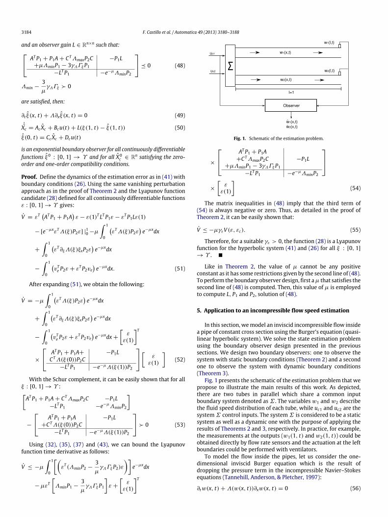
Fig. 1. Schematic of the estimation problem.

×

ATP1 + P1A+CTΛmaxP2C −P1L

+µΛminP1 − 3γΛΓξP1−LTP1 −e−µΛminP2

×

ε

ε(1)

(54)

The matrix inequalities in (48) imply that the third term of(54) is always negative or zero. Thus, as detailed in the proof ofTheorem 2, it can be easily shown that:

V ≤ −µγεV (ε, εc). (55)

Therefore, for a suitable γε > 0, the function (28) is a Lyapunovfunction for the hyperbolic system (41) and (26) for all ξ : [0, 1]→ Υ . �

Like in Theorem 2, the value of µ cannot be any positiveconstant as it has some restrictions given by the second line of (48).To perform the boundary observer design, first aµ that satisfies thesecond line of (48) is computed. Then, this value of µ is employedto compute L, P1 and P2, solution of (48).

5. Application to an incompressible flow speed estimation

In this section, wemodel an inviscid incompressible flow insidea pipe of constant cross section using the Burger’s equation (quasi-linear hyperbolic system). We solve the state estimation problemusing the boundary observer design presented in the previoussections. We design two boundary observers: one to observe thesystem with static boundary conditions (Theorem 2) and a secondone to observe the system with dynamic boundary conditions(Theorem 3).

Fig. 1 presents the schematic of the estimation problem that wepropose to illustrate the main results of this work. As depicted,there are two tubes in parallel which share a common inputboundary system denoted as Σ . The variables w1 and w2 describethe fluid speed distribution of each tube, while uc1 and uc2 are thesystem Σ control inputs. The system Σ is considered to be a staticsystem as well as a dynamic one with the purpose of applying theresults of Theorems 2 and 3, respectively. In practice, for example,the measurements at the outputs (w1(1, t) and w2(1, t)) could beobtained directly by flow rate sensors and the actuation at the leftboundaries could be performed with ventilators.

To model the flow inside the pipes, let us consider the one-dimensional inviscid Burger equation which is the result ofdropping the pressure term in the incompressible Navier–Stokesequations (Tannehill, Anderson, & Pletcher, 1997):

∂tw(x, t) + Λ(w(x, t))∂xw(x, t) = 0 (56)

F. Castillo et al. / Automatica 49 (2013) 3180–3188 3185

where w = [w1, w2]T and

Λ(w) =

w1(x, t) 0

0 w2(x, t)

. (57)

Let us assume that (57) satisfies Assumption 1. Define thefollowing change of coordinates:

ξ1 = w1 − w1, ξ2 = w2 − w2 (58)

where w = [w1, w2]T is an arbitrary reference. With these new

coordinates (ξ1, ξ2), system (56) can be rewritten in the quasi-linear hyperbolic form (1) as follows:

∂t

ξ1ξ2

+

ξ1 + w1 0

0 ξ2 + w2

∂x

ξ1ξ2

=

00

. (59)

Consider the dynamic boundary conditions according to (5)with the respective matrices given by:

A =

−11 45 −8

, B =

8 64 10

,

C = I2, D = 02×2(60)

and also consider the static boundary conditions given by:

ξ(0, t) = −CA−1Buc(t). (61)

Note that due to (60), there is a coupling between thecontrol inputs and the boundary conditions. The static boundaryconditions (61) are chosen such that the obtained flow speeds havesimilar magnitudes as in the dynamic case, allowing to perform acomparison using the same uc for both cases. We require, for theboundary observer design, the definition of the subset Υ as wellas a Lipschitz constant according to (34) and (35), respectively. Wedefine w = [7, 5]T . To build the subset Υ , let us first establish theallowable flow speeds variation as ±0.6 which gives:

w1 ∈ [6.4, 7.6] → ξ1 ∈ [−0.6, 0.6]w2 ∈ [4.4, 5.6] → ξ2 ∈ [−0.6, 0.6].

(62)

From (34), the subset Υ can be defined as:

Υ := {B(0.6) × B(0.6)}. (63)

Due to (57), the Lipschitz constant is γΛ = 1. From (62), thecharacteristic matrix Λ(ξ) can be bounded according to (37) with:

Λmin =

6.4 00 4.4

, Λmax =

7.6 00 5.6

. (64)

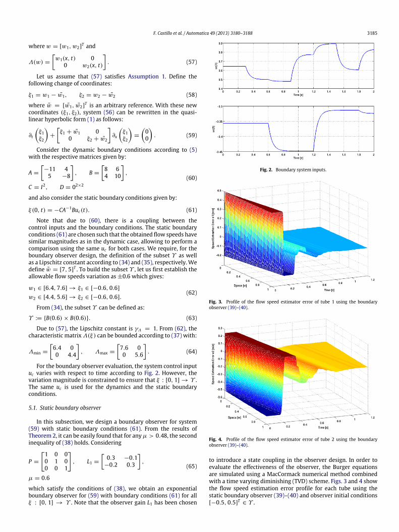
For the boundary observer evaluation, the system control inputuc varies with respect to time according to Fig. 2. However, thevariation magnitude is constrained to ensure that ξ : [0, 1] → Υ .The same uc is used for the dynamics and the static boundaryconditions.

5.1. Static boundary observer

In this subsection, we design a boundary observer for system(59) with static boundary conditions (61). From the results ofTheorem 2, it can be easily found that for anyµ > 0.48, the secondinequality of (38) holds. Considering

P =

1 0 00 1 00 0 1

, L1 =

0.3 −0.1

−0.2 0.3

,

µ = 0.6

(65)

which satisfy the conditions of (38), we obtain an exponentialboundary observer for (59) with boundary conditions (61) for allξ : [0, 1] → Υ . Note that the observer gain L1 has been chosen

Fig. 2. Boundary system inputs.

Fig. 3. Profile of the flow speed estimator error of tube 1 using the boundaryobserver (39)–(40).

Fig. 4. Profile of the flow speed estimator error of tube 2 using the boundaryobserver (39)–(40).

to introduce a state coupling in the observer design. In order toevaluate the effectiveness of the observer, the Burger equationsare simulated using a MacCormack numerical method combinedwith a time varying diminishing (TVD) scheme. Figs. 3 and 4 showthe flow speed estimation error profile for each tube using thestatic boundary observer (39)–(40) and observer initial conditions[−0.5, 0.5]T ∈ Υ .

3186 F. Castillo et al. / Automatica 49 (2013) 3180–3188

Fig. 5. The time evolution of the observer input v(t).

Fig. 6. Time evolution of the Lyapunov function for the static boundary conditions.

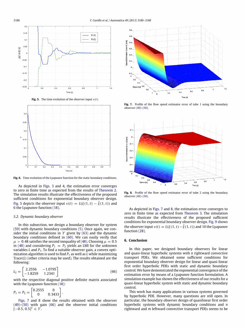
As depicted in Figs. 3 and 4, the estimation error convergesto zero in finite time as expected from the results of Theorem 2.The simulation results illustrate the effectiveness of the proposedsufficient conditions for exponential boundary observer design.Fig. 5 depicts the observer input v(t) = L(ξ(1, t) − ξ (1, t)) and6 the Lyapunov function (18).

5.2. Dynamic boundary observer

In this subsection, we design a boundary observer for system(59) with dynamic boundary conditions (5). Once again, we con-sider the initial conditions in Υ given by (63) and the dynamicboundary conditions defined in (60). We can easily verify thatµ > 0.48 satisfies the second inequality of (48). Choosingµ = 0.5in (48) and considering P1 = P2 yields an LMI for the unknownvariables L and P1. To find a suitable observer gain, a convex opti-mization algorithm is used to find P1 as well as Lwhile maximizingTrace(L) (other criteria may be used). The results obtained are thefollowing:

L2 =

2.2556 −1.0795

−1.8259 1.2341

(66)

with the respective diagonal positive definite matrix associatedwith the Lyapunov function (18):

P1 = P2 =

0.2555 0

0 0.3433

.

Figs. 7 and 8 show the results obtained with the observer(49)–(50) with gain (66) and the observer initial conditions[−0.5, 0.5]T ∈ Υ .

Fig. 7. Profile of the flow speed estimator error of tube 1 using the boundaryobserver (49)–(50).

Fig. 8. Profile of the flow speed estimator error of tube 2 using the boundaryobserver (49)–(50).

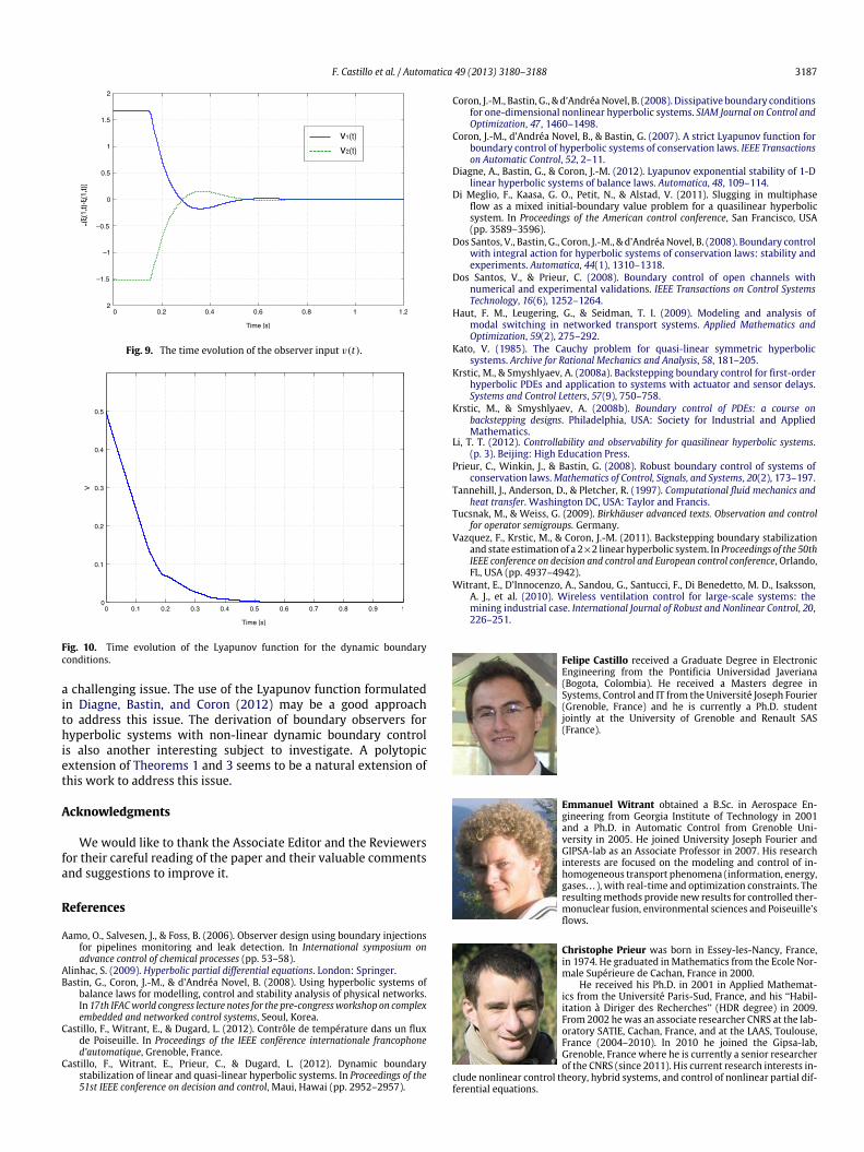
As depicted in Figs. 7 and 8, the estimation error converges tozero in finite time as expected from Theorem 3. The simulationresults illustrate the effectiveness of the proposed sufficientconditions for exponential boundary observer design. Fig. 9 showsthe observer input v(t) = L(ξ(1, t)− ξ (1, t)) and 10 the Lyapunovfunction (28).

6. Conclusion

In this paper, we designed boundary observers for linearand quasi-linear hyperbolic systems with n rightward convectivetransport PDEs. We obtained some sufficient conditions forexponential boundary observer design for linear and quasi-linearfirst order hyperbolic PDEs with static and dynamic boundarycontrol.Wehavedemonstrated the exponential convergence of theestimation error by means of a Lyapunov function formulation. Asimulation example has shown the effectiveness of our results for aquasi-linear hyperbolic system with static and dynamic boundarycontrol.

This work has many applications in various systems governedby hyperbolic PDE. However, many questions are still open. Inparticular, the boundary observer design of quasilinear first orderhyperbolic systems with dynamic boundary conditions and nrightward and m leftward convective transport PDEs seems to be

F. Castillo et al. / Automatica 49 (2013) 3180–3188 3187

Fig. 9. The time evolution of the observer input v(t).

Fig. 10. Time evolution of the Lyapunov function for the dynamic boundaryconditions.

a challenging issue. The use of the Lyapunov function formulatedin Diagne, Bastin, and Coron (2012) may be a good approachto address this issue. The derivation of boundary observers forhyperbolic systems with non-linear dynamic boundary controlis also another interesting subject to investigate. A polytopicextension of Theorems 1 and 3 seems to be a natural extension ofthis work to address this issue.

Acknowledgments

We would like to thank the Associate Editor and the Reviewersfor their careful reading of the paper and their valuable commentsand suggestions to improve it.

References

Aamo, O., Salvesen, J., & Foss, B. (2006). Observer design using boundary injectionsfor pipelines monitoring and leak detection. In International symposium onadvance control of chemical processes (pp. 53–58).

Alinhac, S. (2009). Hyperbolic partial differential equations. London: Springer.Bastin, G., Coron, J.-M., & d’Andréa Novel, B. (2008). Using hyperbolic systems of

balance laws for modelling, control and stability analysis of physical networks.In 17th IFACworld congress lecture notes for the pre-congressworkshop on complexembedded and networked control systems, Seoul, Korea.

Castillo, F., Witrant, E., & Dugard, L. (2012). Contrôle de température dans un fluxde Poiseuille. In Proceedings of the IEEE conférence internationale francophoned’automatique, Grenoble, France.

Castillo, F., Witrant, E., Prieur, C., & Dugard, L. (2012). Dynamic boundarystabilization of linear and quasi-linear hyperbolic systems. In Proceedings of the51st IEEE conference on decision and control, Maui, Hawai (pp. 2952–2957).

Coron, J.-M., Bastin, G., & d’AndréaNovel, B. (2008). Dissipative boundary conditionsfor one-dimensional nonlinear hyperbolic systems. SIAM Journal on Control andOptimization, 47, 1460–1498.

Coron, J.-M., d’Andréa Novel, B., & Bastin, G. (2007). A strict Lyapunov function forboundary control of hyperbolic systems of conservation laws. IEEE Transactionson Automatic Control, 52, 2–11.

Diagne, A., Bastin, G., & Coron, J.-M. (2012). Lyapunov exponential stability of 1-Dlinear hyperbolic systems of balance laws. Automatica, 48, 109–114.

Di Meglio, F., Kaasa, G. O., Petit, N., & Alstad, V. (2011). Slugging in multiphaseflow as a mixed initial-boundary value problem for a quasilinear hyperbolicsystem. In Proceedings of the American control conference, San Francisco, USA(pp. 3589–3596).

Dos Santos, V., Bastin, G., Coron, J.-M., & d’AndréaNovel, B. (2008). Boundary controlwith integral action for hyperbolic systems of conservation laws: stability andexperiments. Automatica, 44(1), 1310–1318.

Dos Santos, V., & Prieur, C. (2008). Boundary control of open channels withnumerical and experimental validations. IEEE Transactions on Control SystemsTechnology, 16(6), 1252–1264.

Haut, F. M., Leugering, G., & Seidman, T. I. (2009). Modeling and analysis ofmodal switching in networked transport systems. Applied Mathematics andOptimization, 59(2), 275–292.

Kato, V. (1985). The Cauchy problem for quasi-linear symmetric hyperbolicsystems. Archive for Rational Mechanics and Analysis, 58, 181–205.

Krstic, M., & Smyshlyaev, A. (2008a). Backstepping boundary control for first-orderhyperbolic PDEs and application to systems with actuator and sensor delays.Systems and Control Letters, 57(9), 750–758.

Krstic, M., & Smyshlyaev, A. (2008b). Boundary control of PDEs: a course onbackstepping designs. Philadelphia, USA: Society for Industrial and AppliedMathematics.

Li, T. T. (2012). Controllability and observability for quasilinear hyperbolic systems.(p. 3). Beijing: High Education Press.

Prieur, C., Winkin, J., & Bastin, G. (2008). Robust boundary control of systems ofconservation laws.Mathematics of Control, Signals, and Systems, 20(2), 173–197.

Tannehill, J., Anderson, D., & Pletcher, R. (1997). Computational fluid mechanics andheat transfer. Washington DC, USA: Taylor and Francis.

Tucsnak, M., & Weiss, G. (2009). Birkhäuser advanced texts. Observation and controlfor operator semigroups. Germany.

Vazquez, F., Krstic, M., & Coron, J.-M. (2011). Backstepping boundary stabilizationand state estimation of a 2×2 linear hyperbolic system. In Proceedings of the 50thIEEE conference on decision and control and European control conference, Orlando,FL, USA (pp. 4937–4942).

Witrant, E., D’Innocenzo, A., Sandou, G., Santucci, F., Di Benedetto, M. D., Isaksson,A. J., et al. (2010). Wireless ventilation control for large-scale systems: themining industrial case. International Journal of Robust and Nonlinear Control, 20,226–251.

Felipe Castillo received a Graduate Degree in ElectronicEngineering from the Pontificia Universidad Javeriana(Bogota, Colombia). He received a Masters degree inSystems, Control and IT from the Université Joseph Fourier(Grenoble, France) and he is currently a Ph.D. studentjointly at the University of Grenoble and Renault SAS(France).

Emmanuel Witrant obtained a B.Sc. in Aerospace En-gineering from Georgia Institute of Technology in 2001and a Ph.D. in Automatic Control from Grenoble Uni-versity in 2005. He joined University Joseph Fourier andGIPSA-lab as an Associate Professor in 2007. His researchinterests are focused on the modeling and control of in-homogeneous transport phenomena (information, energy,gases. . . ), with real-time and optimization constraints. Theresultingmethods provide new results for controlled ther-monuclear fusion, environmental sciences and Poiseuille’sflows.

Christophe Prieur was born in Essey-les-Nancy, France,in 1974. He graduated inMathematics from the Ecole Nor-male Supérieure de Cachan, France in 2000.

He received his Ph.D. in 2001 in Applied Mathemat-ics from the Université Paris-Sud, France, and his ‘‘Habil-itation à Diriger des Recherches’’ (HDR degree) in 2009.From 2002 hewas an associate researcher CNRS at the lab-oratory SATIE, Cachan, France, and at the LAAS, Toulouse,France (2004–2010). In 2010 he joined the Gipsa-lab,Grenoble, France where he is currently a senior researcherof the CNRS (since 2011). His current research interests in-

clude nonlinear control theory, hybrid systems, and control of nonlinear partial dif-ferential equations.

3188 F. Castillo et al. / Automatica 49 (2013) 3180–3188

Luc Dugard got several degrees from the Institut NationalPolytechnique de Grenoble (Grenoble INP): engineerdegrees in radio electricity (1975) and automatic control(1976). Then, he completed his Ph.D. in Automatic Controlin 1980 and his Thèse d’Etat es Sciences Physiques in1984. He also obtained his Habilitation à Diriger desRecherches (HDR) in 1986. Since 1977, he has beenwith the Laboratoire d’Automatique de Grenoble (since2007, Automatic Control Dept. of GIPSA-lab, Grenoble),a research department of Grenoble INP, associated tothe French research organism ‘‘Centre National de la

Recherche Scientifique’’ and presently works as a CNRS Senior Researcher(Directeur de Recherche CNRS). He was vice head (1991–1998) and head(1999–2002) of the Laboratoire d’Automatique de Grenoble. He was part timeworking at the Ministry of Higher Education and Research as a Chargé de Mission(2003–2007). From 2007 to 2012, he was part timeworking at the AERES (Research

and Higher Education Assessment Agency) in Paris, as a Délégué Scientifique(advisor). He has been the chairman of the TC Linear Control Systems of theInternational Federation of Automatic Control (IFAC) from 2005 to 2011. LucDugard has published more than 100 papers (74) and/or chapters (35) ininternational journals or books, and 275 international conference papers. Hehas advised and/or co-advised 34 Ph.D. students. His main research interestsinclude/have included theoretical and methodological studies in the field ofadaptive identification, estimation and control of (multivariable) systems, robustcontrol (time domain and frequency domain approaches), time delay systems(stability analysis and stabilization). The main control applications are/havebeen oriented towards electromechanical systems (flexible systems, inductionmotors, and electrical networks), process control (paper industry, glass industry,nuclear fusion process control) and automotive systems (suspensions, globalchassis control, common rail systems, and engine control), using advanced controlmethods (adaptive control, multivariable control, robust LPV control, nonlinearcontrol. . . ).