boundary domain integral method for transport phenomena in porous media

INTERNATIONAL JOURNAL FOR NUMERICAL METHODS IN FLUIDSInt. J. Numer. Meth. Fluids 2001; 35: 39–54

Boundary domain integral method for transportphenomena in porous media

R. Jecla,*,1, L. S& kergetb and E. Petresina

a Faculty of Ci6il Engineering, Uni6ersity of Maribor, Smetano6a 17, SI-2000 Maribor, Slo6eniab Faculty of Mechanical Engineering, Uni6ersity of Maribor, Smetano6a 17, SI-2000 Maribor, Slo6enia

SUMMARY

A boundary domain integral method (BDIM) for the solution of transport phenomena in porous mediais presented. The complete, so-called modified Navier–Stokes equations (Brinkman-extended Darcyformulation with inertial term included) have been used to describe the fluid motion in porous media.Velocity–vorticity formulation (VVF) of the conservative equations is employed. In this paper, theproposed numerical scheme is tested on a particular case of natural convection and the results of flowand heat transfer characteristics of a fluid in a vertical porous cavity heated from the side and saturatedwith Newtonian fluid are presented in detail. Copyright © 2001 John Wiley & Sons, Ltd.

KEY WORDS: boundary domain integral method; Brinkman-extended Darcy formulation; natural con-vection; porous media; velocity–vorticity formulation

1. INTRODUCTION

Transport phenomena in porous media arise in many diverse fields of science and engineering,such as hydrology, civil and mechanical engineering, chemical and petroleum engineering. Civilengineering deals, for example, with practical problems like the flow of water in aquifers, themovement of moisture through and under engineering structures, the transport of pollutants inaquifers, and heat transport in thermal insulation.

Over the past decades, porous media have been studied both experimentally and theoreti-cally. With the advent of precise instruments and new experimental techniques, it has becomepossible to measure a wide variety of physical properties of porous media and transportphenomena therein. New computational methods and technologies have also allowed us tomodel and simulate various phenomena in porous media, and thus a deeper understanding ofthese problems is being gained on a perpetual basis.

* Correspondence to: Faculty of Civil Engineering, University of Maribor, Smetanova 17, SI-2000 Maribor, Slovenia.Tel.: +386 62 2294322; fax: +386 62 224179.1 E-mail: [email protected]

Copyright © 2001 John Wiley & Sons, Ltd.Recei6ed July 1999

Re6ised December 1999

R. JECL, L. S& KERGET AND E. PETRES& IN40

The term porous media usually refers to material consisting of a solid matrix andinterconnected pores. In the present work, we assume that the solid matrix is rigid, and onaccount of the interconnectedness of the pores, the flow of the fluid is allowed to pass throughthe matrix. Transport phenomena are fluid transport processes describing how variousextensive quantities, e.g. velocity, mass and heat, are transported through a porous mediadomain.

When the temperature of the saturated fluid phase in porous media is not uniform, flowsinduced by buoyancy effects occur. These flows, depending on density differences due totemperature gradients and the pertinent boundary conditions, are commonly called free ornatural convection. Due to its numerous applications in energy-related engineering problems,the natural convection is gaining, over the past decade, strongly enhanced interest and hasbecome one of the most commonly studied transport phenomena in porous media. Studieshave been reported dealing with different geometries and a variety of heating conditions. Forexample, a vertical cavity in which a horizontal temperature gradient is induced by side wallsmaintained at different temperatures has been analysed [1,2]. Others have examined the naturalconvection in porous layers heated from below [3,4]. In all of these studies, use has been madeof Brinkman-extended Darcy formulation as a governing momentum equation, because inearlier works it has been well established that the pure Darcy law does not give satisfactoryresults when one wants to take into account the no-slip boundary condition [5].

The numerical methods often used for the solution of governing equations, which in mostcases are written in vorticity–stream function formulation, are the finite difference method(FDM) and the finite volume method (FVM). The objective of the present work is to examinethe Brinkman-extended Darcy formulation with the transport term included as applied to thecase of natural convection in porous cavity heated from the side, utilizing an approach basedon the boundary domain integral method (BDIM) [6]. The main advantage of the proposedBDIM scheme, as compared with classical domain-type numerical techniques, is that it offersan effective way of dealing with boundary conditions on the solid walls when solving thevorticity equation. Namely, the boundary vorticity in the BDIM is computed directly from thekinematic part of the computation (as described by the Equation (4)) and not through the useof some approximate formulae.

2. GOVERNING EQUATIONS

In principle, the equations that formulate various transport phenomena in porous media areknown and may be written at the microscopic level. However, at this level they can not besolved, as the geometry of the surface that bounds the phase is not observable and/or is toocomplex to be described adequately [7]. Another level of description is therefore needed;namely, the macroscopic level, at which the measurable, continuous and differentiable quanti-ties may be determined and boundary value problems can be stated and later solved. Themacroscopic constitutive equations for the multiphase system, called porous media, areobtained by averaging the governing microscopic equations valid for pure fluid over therepresentative elementary volume (REV), keeping in mind that only the distinct part of theREV (expressed with porosity f) is available for the fluid flow [8]. The averaging process over

Copyright © 2001 John Wiley & Sons, Ltd. Int. J. Numer. Meth. Fluids 2001; 35: 39–54

BDIM FOR TRANSPORT PHENOMENA 41

suitable REV, which has to be determined such that, irrespective of its position in porousmedia, it always contain both a persistent solid and a fluid phases, results in the system ofgoverning equations describing transport phenomena in porous media which consists of

continuity equation

(6i(xi

=0 (1)

momentum equation—Brinkman equation

1f

(6i(t

+1

f2

(6j6i(xj

= −1r

(P(xi

+Fgi−g

K6i

¿¹¹¹¹¹Ë¹¹¹¹¹ÀDarcy law

+g

f

(26i(xj (xj

+1f

(

(xj

(2g¦sij)¿¹¹¹¹¹¹Ë¹¹¹¹¹¹À

Brinkman extension

(2)

energy equation

s(T(t

+(6jT(xj

= ap

(2T(xj (xj

+(

(xj

�a¦p(T(xj

�(3)

where 6i, f, K are filtration velocity, porosity and permeability of porous media respectively.The vector field functions gi and xi represent gravity and position, while the scalar quantitiesP=p−rgiri and T are modified pressure and temperature. The material property r describesthe mass density, assumed to be a constant, and sij stands for the strain rate tensor,sij=

12((6i/(xj+(6j/(xi). The normalized density–temperature variation function F is written as

F= (r−r0)/r0= −bT(T−T0), with r0 denoting the reference mass density at temperature T0

and bT being the thermal volume expansion coefficient. The material property g=m/r is thekinematic viscosity and is partitioned into its constant and perturbated part as g= g+g¦.Coefficient s represents the ratio between the volumetric heat capacity of solid and fluidphases and reads s=f+ (rscs/rc)(1−f), where rs and cs stand for mass density and specificisobaric heat of (only) the solid part of porous media. Finally, the coefficient ap is the constantpart of thermal diffusivity and a¦p is the perturbated part of thermal diffusivity, such thatap= ap+a¦p, where thermal diffusivity is calculated as ap=lp/rc, and lp is the heat conductiv-ity of porous media defined as lp= (1−f)ls+fl, with ls denoting a heat conductivity of thesolid.

As is known, the Brinkman extension expresses the viscous resistance or viscous drag forceexerted by the solid phase on the flowing fluid at their contact surfaces. With the Brinkmanequation one is able to satisfy the no-slip boundary conditions on an impermeable surface,which bounds the porous media. The novelty in our work is that the Brinkman term, asappearing in Equation (2), consists of two parts. The first part, well known in the literature,is a constant and the second one consists of the term that enables us to include the possibilityof general viscosity variation in the computation, a fact of particular importance when dealingwith non-Newtonian saturating fluids. It is important to stress that the Brinkman equation isessentially an interpolation scheme between the Navier–Stokes and Darcy equations. It is well



known [2–8] that, in the limit when the porosity approaches unity (f�1) and consequentlythe permeability tends towards infinity (K��), the Brinkman equation transforms into theclassical Navier–Stokes equation for a pure fluid. Meanwhile, for the permeability convergingto zero (K�0), the Brinkman term becomes negligible and the Darcy law is than recovered.

Due to the general complexity of transport phenomena in porous media we have utilizedcertain assumptions and suppositions as follows:

– the solid phase of the porous media is homogeneous, isotropic and non-deformable (i.e.rigid) substance;

– the fluid phase is described as an incompressible, viscous, single phase;– porous media are saturated—meaning that the fluid occupies the entire void space;– the two average temperatures, Ts for the solid phase and Tf for the fluid phase, are assumed

to be identical in the same REV, so that the thermal behaviour of the porous media isdescribed by a single equation for the average temperature T Ts Tf.

In the BDIM, the obtained set of partial differential equations (PDEs) (1–3), also called themodified Navier–Stokes equations, are further transformed by using the velocity–vorticityvariables formulation (VVF) [9]. With the vorticity vector vi representing the curl of thevelocity field

vi=eijk

(6k(xj

(4)

where eijk is the unit permutation tensor, the fluid motion computation scheme is partitionedinto its kinematic part, as given by the elliptic velocity vector equation

(26i(xj (xj

+eijk

(vk

(xj

=0 (5)

and its kinetic part, as provided by the parabolic–hyperbolic vorticity transport equation,obtained as curl of the momentum equation (2)

(vi

(t6+6j(vi

(xj

=fg(2vi

(xj (xj

+f2eijkgk

(F(xj

+vj

(6i(xj

−f2g

Kvi+f

(

(xj

�g¦(vi

(xj

�+(fij

(xj

(6)

The t6 is so called modified vorticity time step t6= t/f, introduced only as a necessarymathematical step allowing one to use the VVF principle on our momentum equation. Thequantity fij in the last term of Equation (6) is defined as fij=fg¦(9a ×sij).

To improve convergence and stability of the coupled velocity–vorticity iterative numericalscheme, the false transient approach [10] is applied to Equation (5), resulting in the followingparabolic kinematic expression:

(26i(xj (xj

−1a

(6i(t

+eijk

(vk

(xj

=0 (7)



where a is a relaxation parameter. It is obvious that the governing velocity equation (5) isexactly satisfied only in the steady state (t��), i.e. when the artificial time derivative termsvanish.

The boundary conditions assigned to the elliptic kinematic velocity equation (5) aregenerally of the first and second kind

6i= 6i on G1;(6i(xj

nj=(6i(n

on G2 (8)

The Diriclet boundary conditions arise when the velocity is prescribed over the whole surface.In this case, normal derivatives of the velocity components are the unknown boundary valuesin the set of kinematic equations, assuming known vorticity distribution in the solutiondomain. Additional difficulties appear when the velocity vector is not known a priori over partof the surface, i.e. outflow regions. In such cases, a reasonable choice is to assume zero velocitynormal flux values through the specific part of the boundary.

The most critical computation part of the kinematics is the determination of the newboundary vorticity values, which are the only proper physical boundary conditions associatedwith the parabolic kinetic equation (6), as written for the whole boundary

eijk

(6k(xj

=vi on G (9)

while the vorticity normal fluxes

(vi

(xj

nj=(vi

(non G (10)

are the only unknown boundary values in the vorticity kinetics.The mathematical description of the energy kinetics is completed by providing suitable

natural and essential boundary conditions as well as some initial conditions

T=T( on G1; −lp

(T(xj

= q on G2; T=T( 0 in V (11)

3. BOUNDARY DOMAIN INTEGRAL EQUATIONS

3.1. General non-linear parabolic diffusion–con6ecti6e equation

Consider a non-linear time dependent diffusion–convective equation for an arbitrary conserva-tive scalar field function u (velocity, vorticity, temperature) in the form

DuDt

=(u(t

+6j(u(xj

=(

(xj

�a(u(xj

�+Iu (12)



where D/Dt represents the substantial or Stokes derivative and Iu is the source term.Substituting the expression for the diffusivity variation in the form of a constant a and variablepart a¦, so that a= a+a¦, Equation (12) may be partitioned into a linear and non-linear partsin the following manner:

(u(t

+6j(u(xj

= a(2u(xj (xj

+(

(xj

�a¦(u(xj

�+Iu (13)

The equation represents a parabolic initial-boundary value problem; thus some boundary andinitial conditions have to be known a priori in order to complete the mathematical descriptionof the problem

u= u on G1; −k(u(xj

= q on G2; u= u0 in V (14)

The parameters a and k are defined according to the considered conservation laws andcorresponding constitutive hypothesis.

In the transformation from PDEs to integral equations, we consider two different non-ho-mogenous equations, namely the modified Helmholtz PDE for the kinematic and diffusion–convective PDE for the kinetic part of the computation.

By using a finite difference approximation for the time derivative of the field function, wherethe time increment is defined as Dt= tF− tF−1, one has

(u(t:

uF−uF−1

Dt(15)

and Equation (13) can be rewritten in a non-homogenous modified Helmholtz PDE form [9],with the following corresponding integral representation:

c(j)u(j)+&

Gu(u*(n

dG

=1a&

G

�a(u(n

−u6n�

u* dG+1a&

V

�u6j−a¦

(u(xj

� (u*(xj

dV+1a&

VIuu* dV+b

&V

uF−1u* dV

(16)

where the variable u* is the modified Helmholtz fundamental solution [11].The most adequate and stable integral representation could be formulated by using the

fundamental solution of steady diffusion–convective PDE with reaction term [12]. Since itexist only for the case of constant coefficients, the velocity field has to be decomposed into anaverage constant vector 6i and a perturbated vector 6¦i , such that 6i= 6i+6¦i . Once again, theuse of a non-symmetric finite difference approximation of the time derivative permits one torewrite Equation (13) into the non-homogenous diffusion–convective PDE [12], with thefollowing corresponding integral formulation:



c(j)u(j)+&

Gu(U*(n

dG=1a&

G

�a(u(n

−u6n�

U* dG+1a&

V

�u6¦j −a¦

(u(xj

� (U*(xj

dV

+1a&

VIuU* dV+b

&V

uF−1U* dV (17)

with U* being the product of the diffusion–convective fundamental solution and the constantpart of diffusivity as U*= au*, where u* is the fundamental solution of the steady diffusion–convective PDE with first-order reaction term [11].

3.2. Modified Na6ier–Stokes equations

The integral representation of the modified Navier–Stokes equations for the conservative fieldfunctions, i.e. velocity, vorticity and temperature, can be readily obtained following theintegral statements developed above for the general transport equation (13).

As computational results in the present work are limited to the two-dimensional case, all thesubsequent equations will consequently be written for the case of a planar geometry only.Considering that each component of the velocity vector 6i, Equation (7), satisfies the non-ho-mogenous modified Helmholtz PDE subject to the corresponding boundary and initialconditions, as given by Equation (8), applying the integral formulation given by Equation (16),we obtain the boundary-domain integral statement for the planar flow kinematics

c(j)6i(j)+&

G6i(u*(n

dG=&

G

�(6i(n

+eijvnj�

u* dG−eij&

Vv(u*(xj

dV+b&

V6i,F−1u* dV

(18)

describing the time-dependent transport of velocity field 6i in porous media. Parameter b isdefined as b=1/aDt and u* is the modified Helmholtz fundamental solution [13], which takesinto account the effects of geometry, time step and material properties.

Considering that the vorticity v and temperature T, as described by Equations (6) and (3),obey the non-homogenous diffusion–convective PDE, subject to the normal, essential andinitial conditions as given by Equations (9)–(11) respectively, applying the integral formulationas given by Equation (17), we obtain the boundary-domain integral statement for the planar6orticity kinetics

c(j)v(j)+&

Gv(U*(n

dG=1

fg

&G

�fg(v

(n−v6n+f2eijnigjF+ fjnj

�U* dG

+1

fg

&V

�v6¦j −f2eijgjF−fg¦

(v

(xj

− fj� (U*(xj

dV

−1

fg

&V

f2g

KvU* dV+b

&V

vF−1U* dV (19)



describing the time-dependent transport of vorticity v in the porous media domain. Theparameter b is defined as b=1/fgDt6, U*= gfu* and u* is the elliptic diffusion–convectivefundamental solution of the steady diffusion–convective PDE, with first-order reaction term,considering the effects of geometry, material properties, modified vorticity time step andvelocity [13]. Finally, we obtain the boundary–domain integral statement for the planar heatenergy kinetics

c(j)T(j)+&

GT(U*(n

dG

=1ap

&G

�ap

(T(n

−T6n�

U* dG+1ap

&V

�6¦j T−a¦p

(T(xj

� (U*(xj

dV+b&

VTF−1U* dV (20)

describing the time-dependent transport of temperature T in porous media. Here, once againb is defined as b=1/sDtT and tT is the modified temperature time step introduced only forthe proper mathematical treatment of the heat energy equation (3), as tT= t/s. As previously,U*= apu* and u* is the fundamental solution of the steady diffusion–convective PDE with afirst-order reaction term [13].

4. DISCRETIZED BOUNDARY DOMAIN INTEGRAL EQUATIONS

4.1. Formulation for general non-linear partial differential equation

Searching for an approximate numerical solution, the corresponding integral equations arewritten in a discretized manner [14]. The integrals over the boundary and domain areapproximated by a sum of integrals over E individual boundary elements and C internal cellsrespectively. The variation of field functions or their products within each boundary elementor internal cell is approximated by the use of appropriate interpolation polynomials. Afterapplying the discretized integral equations to all subdomain boundary and internal nodes, thefollowing implicit matrix systems can be obtained for the modified Helmholtz PDE:

[H ]{u}= [G ]�a

an!(u(n"

−1a

[G ][6n ]{u}+1a

[Dj ][6j ]{u}− [Dj ]�a¦

an!(u(xj

"+

1a

[B ]{Iu}

+b [B ]{u}F−1 (21)

and for the diffusion–convective PDE:

[H ]{u}= [G ]�a

an!(u(n"

−1a

[G ][6n ]{u}+1a

[Dj ][6¦j ]{u}− [Dj ]�a¦

an!(u(xj

"+

1a

[B ]{Iu}

+b [B ]{u}F−1 (22)

To improve the economics of the computation and thus widen the applicability of theproposed numerical algorithm, the subdomain technique has been chosen [15]. The idea is to



partition the entire solution domain into subdomains to which the same discretized numeri-cal procedure can be applied. The final system of equations for the entire domain is thenobtained by adding the sets of equations for each subdomain considering the compatibilityand equilibrium conditions between their interfaces, resulting in a more sparse matrixsystem, suitable to be solved by iterative techniques. For instance, the following conditionsmay be applied on the interface indicated with G1 between subdomains V1 and V2:

u �I1=u �I2, k(u(n

)I

1

= −k(u(n

)I

2

(23)

The discrete model is based on a substructure technique derived to its limit version follow-ing the concept of finite volume, e.g. that each quadrilateral internal cell represents onesubdomain bounded by four boundary elements. The geometrical singularities are overcomeby using 3-node discontinuous quadratic boundary elements combined with 9-node cornercontinuous internal cells.

4.2. Formulation for modified Na6ier–Stokes equations

The discretized integral representations for the modified Navier–Stokes equations could beobtained by following the solution procedure as developed above for the general conserva-tion field function u. Using the discretized equation (21), having in mind the boundary–domain integral equation (18), the following implicit matrix system is obtained for thekinematic :

[H ]{6i}= [G ]!(6i(n

"+eij [G ]{vnj}−eij [Dj ]{v}+b [D ]{6i}F−1 (24)

to be solved for unknown boundary velocity components or their normal derivatives respec-tively, while the computation of all internal domain velocity components, if needed, isperformed in an explicit manner point by point.

Applying Equation (22) to the corresponding Equations (19) and (20), the implicit matrixsystem for the 6orticity kinetics

[H ]{v}= [G ]�g

g

n!(v(n

"−

1fg

[G ][6n ]{v}+1

fg[Dj ][6¦j ]{v}−

1fg

�f2g

Kn

[B ]{v}

+1

fg[G ]{f2eijnigjF+ fjnj}− [Dj ]

�g¦g

n!(v(xj

"−

1fg

[Dj ]{f2eijgjF+ fj}

+b [B ]{v}F−1 (25)

is obtained to be solved for unknown boundary vorticity flux values and unknown domainvorticity values, while the implicit matrix system for heat energy kinetics



[H ]{T}= [G ]�ap

ap

n!(T(n

"−

1ap

[G ][6n ]{T}+1ap

[Dj ][6¦j ]{T}− [Dj ]�a¦p

ap

n!(T(xj

"+b [B ]{T}F−1

(26)

is recovered in order to determine the unknown boundary temperature flux or boundarytemperature values and temperature internal domain values.

5. SOLUTION PROCEDURE

The kinematics given by Equation (24) and the velocity boundary conditions prescribed byEquation (8) cannot assure a solenoidality of the velocity field for an arbitrary vorticitydistribution, so this property may be fulfilled only by coupling kinetic and kinematicequations. Thus, the solenoidality conditions of the velocity and vorticity field requires acoupled iterative solution of the non-linear dynamic system as given by Equations (24)–(26)with the corresponding boundary conditions described by Equations (9)–(11). To obtain asolution of the fluid motion problem, the following iterative steps have to be performed.

1. Start with some initial values for the vorticity distribution.2. Kinematic computational part:

� solves implicit sets for boundary velocity or velocity normal flux values—Equation (24),� transforms new function values from element nodes to cell nodes,� computes the gradient of the velocity components,� determines new boundary vorticity values—Equation (9),� determines new boundary domain integral kinetic matrices, if the constant velocity

vector is perturbed more than the prescribed tolerance.3. Energy kinetic computational part:

� solves implicit set for boundary and domain values—Equation (26),� transforms new function values from element nodes to cell nodes.

4. Vorticity kinetic computational part:� solves implicit set for unknown boundary vorticity flux and internal domain vorticity

values—Equation (25),� transforms new function values from element nodes to cell nodes.

5. Relaxation of all new values and the convergence examination. If the convergence criterionis satisfied, then stop; otherwise go to step 2.

6. NATURAL CONVECTION IN POROUS CAVITY

To check the validity of proposed numerical procedure we will discuss the problem of naturalconvection in a vertical porous cavity. The description of the physical problem is shown onFigure 1 and represents a two-dimensional, vertical cavity filled with an isotropic, homoge-neous, Newtonian fluid-saturated porous media. One vertical wall of the cavity is isothermallyheated, the other is isothermally cooled, and the horizontal walls are adiabatic.



Figure 1. Geometry and boundary conditions for porous cavity.

The thermo-physical properties of the solid and the fluid are assumed to be constant exceptfor the density variation in the body force term. Assuming that the solid particles and the fluidare in thermal equilibrium, the governing equations are written in the form of Equations(1)–(3). The computations have been carried out for the complete Brinkman-extended Darcymodel with the transport term in the momentum equation included. Whenever we consider theBrinkman term, we have to deal with a parameter called the Darcy number, Da [1], appearingas the ratio between the permeability and the characteristic length multiplied with the viscosityratio L, which is, in our case, equal to the reciprocal value of porosity (L=1/f). We muststress that, with the use of the BDIM, the Darcy number is not explicitly derived as we are notemploying the non-dimensionalized formulation of the governing equations, which is thecommon procedure used with other numerical methods. We will use that parameter only forthe reason of comparison with the published results, noting that the permeability itselfcompletely defines the characteristics of porous media when the BDIM is used. Thus, thegoverning parameters for the present problem are

– porosity f,– modified (porous) Rayleigh number Ra*=gbKDDT/gap,– permeability of porous media K, defined in the terms of the so-called Darcy number as

Da= (1/f)(K/D2),– aspect ratio A=H/D,– ratio between volumetric heat capacity of solid and fluid phase defined as the so-called heat

capacity ratio s=f+ (rscs/rc)(1−f),

where D, H, DT are the width of the cavity, the height of the cavity and the temperaturedifference between hot and cold walls respectively. Parameter b is the isobaric coefficient ofthermal expansion of the fluid.

We have tested our numerical model on several different cases and therefore we can confirmthe findings of others [1,2,5], that the effect of an increase in the Darcy number appears to be



very similar at all modified Rayleigh numbers, although it is known that the effect of theviscous (Brinkman) term becomes more important at high modified Rayleigh numbers. Theproposed BDIM scheme has been verified in a square cavity with aspect ratio A=1 andbecause of the above-mentioned similarity we graphically present only one example, forRa*=500, in order to outline the relevant characteristics that are common to all modifiedRayleigh numbers.

The boundary conditions for computed test examples are

6x= 6y=0 for x=0, D and y=0, H(T(y

=0 for y=0, H

T( =T( H=0.5 for x=0

T( =T( C= −0.5 for x=D

The streamlines and isotherms for a square cavity with aspect ratio A=1, modified Rayleighnumber Ra*=500 and different Darcy numbers Da=10−1, 10−2, 10−3, 10−4, are presented

Figure 2. Streamlines for A=1, f=0.5, DT=1, Ra*=500; (a) Da=10−4, (b) Da=10−3,(c) Da=10−2, (d) Da=10−1.

Figure 3. Isotherms for A=1, f=0.5, DT=1, Ra*=500; (a) Da=10−4, (b) Da=10−3,(c) Da=10−2, (d) Da=10−1.



in Figures 2 and 3. A computational mesh of 10×10 subdomains is used. Time steps rangedfrom Dt=1016 (steady state) for Da=10−1, Dt=10−1 for Da=10−2, Dt=10−2 for Da=10−3 to Dt=10−3 for Da=10−4 and the convergence criterion was selected as o=0.00001.The porosity is equal to f=0.5 and the heat capacity ratio to s=1.

The streamlines in Figure 2(a) are observed to be closely spaced near the solid boundaries.This configuration indicates that the fluid velocity reaches a maximum near the boundaries asexpected, since in the limit when Da=0 (Darcy law), the velocity has a maximum on theboundaries. In this case, Da is small enough so that the viscous term, which is responsible forthe boundary effects, becomes negligible and the Darcy law correctly describes the flowbehaviour. Figure 2(b)–(d) illustrates typical results obtained on the basis of Brinkman modelfor various values of Da. It is evident that when the Darcy number increased, the boundaryeffects on the flow field become significant and the streamlines are observed to becomerelatively more sparsely spaced near the solid boundaries. This is so due to the fact that theviscous term (Brinkman term) becomes gradually more important and slows down the fluid inthe neighbourhood of the solid walls. It is also observed that the region where the flow attainsmaximum velocity, as indicated by closely spaced streamlines, moves away from the wallstowards the core region as Da is increased.

Similarly, we can observe the effects of Darcy numbers on the isotherms or on thetemperature field (Figure 3). When the Darcy number is small—Figure 3(a)—the convectivemotion inside the cavity is strong and the isotherms are considerably distorted. The flatisotherms in the core indicate a negligible lateral conduction. As Da is increased, the viscouseffects become more important and slow down the buoyancy induced flow inside the cavity.The isotherm profiles become more linear and heat transfer across the cavity results from thecombined action of conduction and convection.

From the above-presented results we can clearly observe that the streamlines and isothermsredistribution are almost identical for Da= 10−4 and Da= 10−3, but with a further increasein the Darcy number (that means with an increase in permeability K), the velocity andtemperature fields are starting to becomes significantly modified.

In what follows we will compare our results with the findings of others for which the workof Lauriat and Prasad [1] has been chosen. The rate of heat transfer expressed with the averageNusselt number Nu=0

1 (T/(n dy for different modified Rayleigh numbers are collected inTable I, where in brackets the results from Reference [1] are presented. The straightforwardcomparison is not fully possible because, in above-mentioned study, the authors have calcu-lated the Nusselt number considering the Brinkman momentum equation in which thetransport term had been assumed to be negligible, while in our work the computations havebeen made on the basis of the complete Brinkman equation in the form as given by Equation(2). Also we employ the viscosity ratio L equal to the reciprocal value of porosity [8], whileLauriat and Prasad have taken this ratio equal to unity. Therefore, their results can be usedby replacing the modified Rayleigh number Ra* in their formulation with Ra* multiplied byfactor 2 (f−1=0.5−1=2).

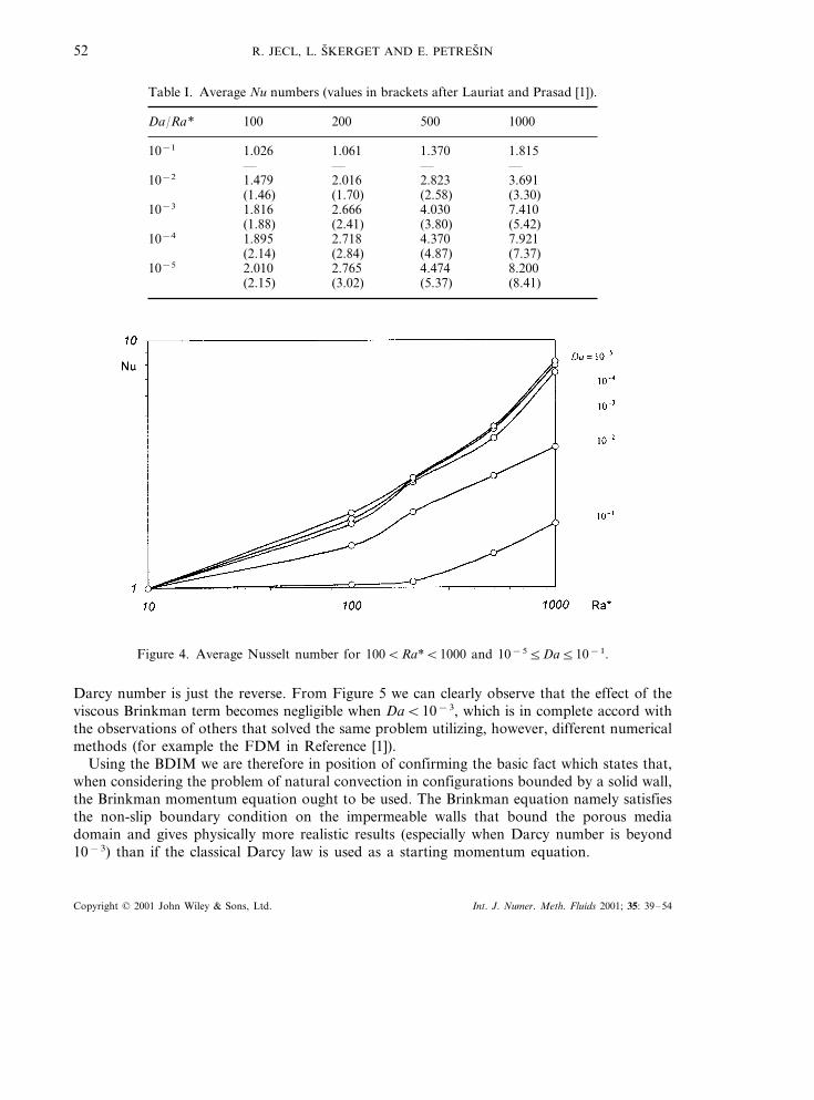
The average Nusselt number is presented in Figures 4 and 5 for A=1, modified Rayleighnumbers Ra*=100, 200, 500 and 1000, and different Darcy Numbers 10−55Da510−1. Asexpected, the Nusselt number approaches the conduction value (Nu=1) when Ra* approacheszero (Ra*�0). Also, the Nusselt number always increases with Ra*, but the effect of the



Table I. Average Nu numbers (values in brackets after Lauriat and Prasad [1]).

100 200Da/Ra* 500 1000

1.026 1.061 1.37010−1 1.815— — — —1.479 2.01610−2 2.823 3.691(1.46) (1.70) (2.58) (3.30)1.816 2.66610−3 4.030 7.410(1.88) (2.41) (3.80) (5.42)1.895 2.71810−4 4.370 7.921(2.14) (2.84) (4.87) (7.37)2.010 2.76510−5 4.474 8.200(2.15) (3.02) (5.37) (8.41)

Figure 4. Average Nusselt number for 100BRa*B1000 and 10−55Da510−1.

Darcy number is just the reverse. From Figure 5 we can clearly observe that the effect of theviscous Brinkman term becomes negligible when DaB10−3, which is in complete accord withthe observations of others that solved the same problem utilizing, however, different numericalmethods (for example the FDM in Reference [1]).

Using the BDIM we are therefore in position of confirming the basic fact which states that,when considering the problem of natural convection in configurations bounded by a solid wall,the Brinkman momentum equation ought to be used. The Brinkman equation namely satisfiesthe non-slip boundary condition on the impermeable walls that bound the porous mediadomain and gives physically more realistic results (especially when Darcy number is beyond10−3) than if the classical Darcy law is used as a starting momentum equation.



Figure 5. Effect of Darcy number on the average Nusselt number.

7. CONCLUSION

A numerical approach based on the BDIM is being applied for the solution of the problem ofnatural convection in porous cavity. The solution is based on the VVF of the modifiedNavier–Stokes equations, which allows the separation of the computational scheme into itskinematic and kinetic part respectively. The elliptic modified Helmholtz fundamental solutionis used for the kinematic part of computation, while the elliptic diffusion–convective funda-mental solution is employed for the kinetic one. The limited version of the subdomaintechnique, e.g. each subdomain is being constructed of four discontinuous 3-node quadraticboundary elements and one continuous 9-node corner continuous quadratic cell, has beenapplied. The proposed numerical procedure is studied, presented and discussed for the case ofnatural convection in porous cavity heated from the side for different Rayleigh and Darcynumbers. The very encouraging results obtained serve as a strong indication that the BDIMpossesses the potential to become a powerful alternative to the existing numerical methods forsolving certain class of transport phenomena in porous media.

REFERENCES

1. Lauriat G, Prasad V. Natural convection in a vertical porous cavity: a numerical study for Brinkman-extendedDarcy formulation. Journal of Heat Transfer 1987; 109: 688–696.

2. Vasseur P, Wang CH, Sen M. Natural convection in an inclined rectangular porous slot: the Brinkman-extendedDarcy model. Journal of Heat Transfer 1990; 112: 507–511.

3. Malmou M, Robillard L, Bilgen E, Vasseur P. Entrainment effect of a moving thermal wave on Benard cells ina horizontal porous layer. In Proceedings of the 2nd International Conference on Ad6anced Computational Methodsin Heat Transfer, Wrobel LC, Brebbia CA, Nowak AJ (eds). CMP: Southampton, 1992; 442–456.



4. Kladias N, Prasad V. Natural convection in horizontal porous layers: effects of Darcy and Prandtl numbers.Journal of Heat Transfer 1989; 111: 926–935.

5. Tong TW, Subramanian E. A boundary-layer analysis for natural convection in vertical porous enclosures—useof the Brinkman-extended Darcy model. International Journal of Heat Mass Transfer 1985; 28: 563–571.

6. S& kerget L, Rek Z. Boundary-domain integral method using a velocity–vorticity formulation. Engineering Analysiswith Boundary Elements 1995; 15: 359–370.

7. Bear J, Bachmat Y. Introduction to Modelling of Transport Phenomena in Porous Media. Kluwer Academic:Dordrecht, 1991.

8. Nield DA, Bejan A. Con6ection in Porous Media. Springer: Berlin, 1992.9. S& kerget L, Alujevic A, Brebbia CA, Kuhn G. Natural and forced convection simulation using the velocity–

vorticity approach. Topics in Boundary Element Research 1989; 5: 49–86.10. Guj G, Stella F. A vorticity–velocity method for the numerical solution of 3D incompressible flows. Journal of

Computational Physics 1993; 106: 286–298.11. S& kerget L, Hribersek M, Kuhn G. Computational fluid dynamics by boundary-domain integral method.

International Journal for Numerical Methods in Engineering 1999; 46: 1291–1311.12. Z& agar I, S& kerget L. Integral formulations of a diffusive–convective transport equation. In BE Applications in Fluid

Mechanics, Power H (ed.). CMP: Southampton, 1995; 153–176.13. Jecl R, S& kerget L. Fluid transport process in porous media using boundary domain integral method. In

Proceedings of the 4th European Computational Fluid Dynamics Conference, Papailiou KD, Tsahalis D, Periaux J,Hirsch C, Pandolfi M (eds). Wiley: Chichester, 1988; 1180–1185.

14. Brebbia CA, Dominquez J. Boundary Elements. An Introductory Course. McGraw-Hill: New York, 1992.15. Hribersek M, S& kerget L. Iterative methods in solving Navier–Stokes equations by the boundary element method.

International Journal for Numerical Methods in Engineering 1996; 39: 115–139.


boundary domain integral method for transport phenomena in porous media

Documents