blume-emery-griffiths model on the honeycomb...

Journal o f Statistical Physics, VoL 50, Nos. 1/2, 1988

Biume-Emery-Griffiths Model on the Honeycomb Lattice

X. N. Wu I and F. Y. Wu 1

Received August 4, 1987

Exact results are obtained for a spin-1 system on the honeycomb lattice with the Blume-Emery~3riffiths Hamiltonian - Yi"/k T = J ~ i , j S i S j My K ~( i , j ) $2 $2 --

A ~ i S 2 + H S ~ S i subject to the constraint K = - l n c o s h J . For J > 0 , the system behaves like a spin-l/2 Ising ferromagnet with the free energy analytic everywhere except at the first-order phase boundary H = 0 , tanh J < (2 + e~)/2x/-J. Derivatives of the free energy across this boundary are discontinuous and we obtain the exact expression for the spontaneous magnetization. For J < 0 , the system can be transcribed into an antiferromagnetic spin-l/2 Ising model in a real magnetic field, and from this equivalence portions of the exact phase boundary are determined.

KEY WORDS: Blume-Emery-Griffiths model; honeycomb lattice; spontaneous magnetization; exact results.

1. I N T R O D U C T I O N

The Blume-Emery-Griffiths (BEG) model (1) is a spin-1 system with dipolar and quadrupolar exchange interactions. The BEG Hamiltonian

-H/kT=J Z $5/+K Z S2iS2-A~S~+H~,Si ( i , j ) ( i , . j ) i i

(1)

where Si=0, +1 was first proposed to explain certain magnetic transitions. (241 But the Hamiltonian (1) has also proven to be useful for modeling the 2 transition and phase separation in 3He-4He mixtures (1) and, more recently, the phase changes in a microemulsionJ 5) In these and other studies of the BEG model, extensive analyses have been carried out using the renormalization group (6) and mean-field (7) approximations in the

1 Department of Physics, Northeastern University, Boston, Massachusetts 02115.

41

0022-4715/88/0100-0041506.00/0 re? 1988 Plenum Publishing Corporation

42 Wu and Wu

ferromagnetic regime J > 0 , K > 0 and the antiferromagnetic regime J < 0 , K=0 . ~8) In addition, a few exact results are known. These include the equivalence with a spin-l/2 Ising model in a nonzero magnetic field for J : H - - - - 0 (9) and J - 0 , H:~O, (1~ and the recently obtained solution of the BEG model on the honeycomb lattice in the subspace

K = - l n cosh J (2)

for H = 0 (11'~2) and H = i~. (13) The tricritical point behavior of the BEG model has been reviewed by Lawrie and Sarbach/14)

In this paper we consider the general BEG model (1) on the honeycomb lattice in the subspace (2) for arbitrary J, H, and A. We show that this BEG model is also equivalent with an Ising model in an external magnetic field, an equivalence which permits us to establish a number of analytic properties for the BEG model. Our method of analysis makes use of results of an eight-vertex model on the honeycomb lattice considered by Wu. (~5) However, details of some crucial steps of the analysis were not given in Ref. 15. These steps are now presented, together with further new results on the equivalence.

The paper is organized as follows. In Section 2 we analyze the ground state of the BEG model (1) and (2), and in Section3 we establish the equivalence of the BEG model with an eight-vertex model. Section 4 is a self-contained analysis of the eight-vertex model, establishing its equivalence with an Ising model, an analysis which goes beyond that given in Ref. 15. This formulation of the eight-vertex model is applied to the BEG model in Section 5, and we discuss analytic properties of the BEG model in Sections 6 and 7 for the cases of J > 0 and J < 0, respectively.

2. G R O U N D STATE OF THE BEG M O D E L

In this section we analyze the ground state of the BEG model (1) and (2). In the limit of T ~ 0 and using (2), we may replace

K--, -IJI (3)

in (1). It is then convenient to consider the two cases J > 0 and J < 0 separately.

2.1. Ferromagnet ic Case ( J > 0)

For J > 0 the ground-state energy is given by, in units of JkT,

~P ~ ( S i S j _ S i S j ) ..~ 2 A~/ ~H~/ --* S/2 ----7 Si (4) ( i , j )

BEG Model on the Honeycomb Lattice 43

12

,

9

\

", (a): =01 %

\ 3

x

- 9 - 6 - 3 ~ \ ( / /

I 0

(e): {si=-l~

/ /

/ /

/ /

1 i

i /

/ /

/ 1

/

3 6 9 1 2

I I ~ " H-j/

(1): ~si=+l]

- 6

- 9

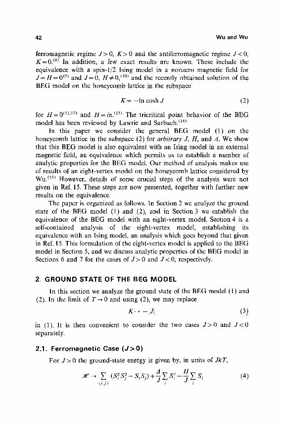
Fig. 1. The three ground-state regimes for J > 0. The phase boundaries indicated by broken lines do not extend into nonzero temperatures.

It is then straightforward to compare energies of ordered states and to see that the ground state can be one of three states with all spins equal to S i = t , - 1, or 0. The regimes in the parameter space in which these ordered states prevail are indicated by 1-3, respectively, in Fig. 1. While we generally expect the phase boundaries in the ground state of a spin system to extend into nonzero temperatures, we shall see later that the boundaries between regime 3 and regimes 1 and 2, denoted by broken lines, are special and do not extend into nonzero temperatures, a reflection of the fact that the surface tension vanishes exactly along these boundaries. 2 But the boundary H = 0 between regimes 1 and 2 does extend into nonzero temperature, becoming a first-order surface.

2.2. A n t i f e r r o m a g n e t i c Case ( J < 0)

For J < 0 the ground-state energy is given by, in units of ]JlkT,

A H

< i , j > " "

Comparison of the energies of the ordered states then leads to six possible ground states. These include the three states in which all spins are 1, - 1 ,

2 We are indebted to Professor Michael Schick for this remark.

44 Wu and Wu

- 1 2

I

~/lal

6 @ %.~ (3): ~s~;ol / x•

\"'%. \ f'/ / \ %,_ \ / / @" /

; r162

Y I''r (~)'.Is~=-q ..I I (1):~,=+II

- I (8): I..

(+)1 ? -6 I (+) I~s~,sJ=!+ l , - i )~

- 9

12

'~ H/IJI

Fig. 2. The six ground-state regimes for J< 0. The phase boundaries indicated by broken lines do not extend into nonzero temperatures.

or 0, as well as the three states in which nearest neighboring pairs are {1, 0}, { - 1 , 0}, and {1, - 1 } . The six regimes are indicated by 1, 2 ..... 6, respectively, in Fig. 2. We shall see later that all phase boundaries, except the two segments denoted by broken lines between regime 6 and regimes 4 and 5, extend to nonzero temperatures.

3. EQUIVALENCE OF THE BEG M O D E L W I T H AN E I G H T - V E R T E X M O D E L

In this section we show that the BEG model (1) and (2) is reducible to an eight-vertex model.

Consider the BEG model (1) on a honeycomb lattice of N sites with the interaction parameters J and K related by (2). In this paper we restrict our considerations to the physical regime when all parameters J, K, A, H are real, although much of our discussions are valid more generally, including complex interactions. By symmetry there is no loss of generality to take H > 0. Interactions J and A can be either positive or negative, and K is always negative, as implied by (2).

It is readily verified, using (2), that we have the identity

exp(JSiSj + KS~ S 2) = 1 + SiSy tanh J (6)


J : .SA. ', , ,, . ~ . . . . . , , , , , . . . . - ~ ~ . . . . . o . . o .

a b b b e e e d

Fig. 3. The eight vertex configurations of the eight-vertex model and the vertex weights.

Then the partition function of the BEG model can be rewritten as

ZBEG = Y', 1-[ ( l + S , S j tanhJ) l - [exp(-AS2+HS~) (7) S i=O• 1 ( i , j ) i

Expand the product over neighboring pairs in (7) and represent each term in the expansion by a graph drawn on the lattice. For each tanh J and the associated SeSj factor we draw a bond between sites i and j. This leads to eight different kinds of configurations, shown in Fig. 3, that can occur at a vertex. Furthermore, by carrying out the spin sums at each vertex and associating a factor (tanh j ) m to each half of a bond incident to a vertex, we can associate weights to vertices. This leads to the consideration of an eight-vertex model on the honeycomb lattice with vertex weights

a = ~. e ~ s 2 + H S = l + 2 e ~ c o s h H S = 0 , + I

b = t 1/2 ~ . S e _as2+ Hs = 2tl/2e-A sinh H S = 0 , + I

c = t ~. S2e-~S2+ns=2te A c o s h H (8) S = O , + I

d= t 3/2 ~ S3e -AS2+Hs= 2t3/2e ~ s inhH S - - O , + l

where

t -= tanh J

Thus, we have established the identity

ZBEO = Zsv(a, b, c, d) (9)

where Zsv(a , b, c, d) is the partition function of the eight-vertex model. For J > 0, the vertex weights a, b, c, and d are positive and we may use results of Ref. 15. For J < 0, however, the weights b and d are pure imaginary, and this leads to a situation different from that of Ref. 15.

46 Wu and Wu

4. EQUIVALENCE OF THE EIGHT-VERTEX M O D E L W I T H AN ISING M O D E L

This section is a self-contained analysis of the eight-vertex model on the honeycomb lattice, establishing its complete equivalence with an Ising model in a nonzero external field. (15) Some steps of the analysis are already given in Ref. 15, but many results presented here are new. This section is written as much as possible without reference to the BEG model, and can be regarded as an independent section.

The equivalence of the two models is deduced by applying a weak- graph expansion to the partition function Z8v(a, b, c, d). The weak-graph expansion is a linear transformation of the vertex weights described by

gz = (a + 3yb + 3y2c + y3d)/(1 + y2)3/2

T) = [ya - (1 - 2y2)b + (y3 _ 2y)c -- y2d]/(1 + y2)3/2 (lO)

? = [y2 a + (y3 _ 2y)b + (1 - 2y2)c + yd]/(1 + y2)3/2

~= (y3a-- 3y2b + 3 y c - d ) / ( 1 + y2)3/2

under which the partition function of the vertex model remains invariant. (15) That is,

Zsv(a, b, c, d) = Zsv(t~, b, 8, ~) (11)

However, the transformation (10) contains a parameter y at disposal, which we can choose at our convenience. For our purposes it is most convenient to choose y to satisfy

~d=be (12)

When (12) holds, the eight-vertex partition function is related to an Ising partition function as described in the following.

Consider a spin-l/2 Ising model on the same honeycomb lattice with the partition function

Z,(L, K,) = Z ~I eKI~e~J 1-[ ec~ (13) ~r n n i

Then, expanding (13) into a high-temperature expansion and considering the resulting expression as an eight-vertex model partition function, one obtains (15)

Zsv(& b, g, ~) = (fi/2 cosh L)~V(cosh K,) -3N/2 Z i ( t , K,) (14)


with the Ising parameters given by

tanh K~ = ?/a (15)

tanh L = ~/(ag)m (16)

It is readily verified using (10) that

~t~-bg= [By2 + 2(A + C) y - B]/(1 + y2) (17)

where

A=_c2-bd, B=_ad-bc, C = a c - b 2 (18)

Therefore, the condition (12) leads to the quadratic equation for y,

By2 + 2(A + C) y - B=O (19)

with the solutions

where

y = y_+ = [ - ( A + C)+6]/B

6 - [(A + C)2+B2] 1/2

(20)

(21)

The choice of the sign in (20) is arbitrary. This means that there exist two weak-graph transformations leading to two sets of Ising parameters (and the same Ising partition function), which we can choose at our convenience.

Using (19) and (20), it is straightforward to show that (10) can be rewritten as

= FU/BD, ~ = FV/BD, ~ = GU/BD, ~= GV/BD (22)

where

F - y(By + 2C) G =- y(By + 2A)

U = - ( b + d ) y + a + c , V = - ( a + c ) y - ( b + d ) (23)

D = (1 + y2)3/2

Furthermore, (15) and (16) lead to

eZtq = By + C + A tanh L = V (By + 2C~ 1/2 C - A ' -~ \--fff -~-~-~ / (24)

822/50/1-2-4

48 Wu and Wu

The substitution of the two values of y = y + into (24) now leads to the two sets of Ising parameters

exp(2K~+ ) = +_6/(C- A) (25)

V+(+f-A+C) 1/2 tanh L + = ~ \ ~ 6 + A - - (26)

where the + signs refer to the use of y = y+ in each expression. [ F o r example, U+ = (b + d) y + + a + c, etc. ]

The two sets of Ising parameters are not independent. Using (25) and the identity U+ U_ = - V + V , one verifies that they are related by

tanh KI+ tanh Ki_ = 1, tanh L + tanh L _ = 1 (27)

or, equivalently,

e 2K'+ = - e 2K'-, e 2c§ = - e 2c (28)

It can be easily seen that these two sets of Ising parameters lead to the same Ising part i t ion function. In fact, it can be more generally shown that 3

(29) , , ,

from which (27) and (28) follow directly from (15) and (16). For A and C real and 6 positive, as is the case in our application (Sec-

tion 5 below), the Ising parameter K~ is real if we take

{y, K, , L} = { y + , L + ), C - A > O (30)

={y_,KI ,L_}, C--A<O

In our application (Section 5) the Ising magnetic field L in (30) also turns out to be real. We shall therefore use (30) to define the Ising parameters, which are always real. 4

In the determinat ion of the critical point of the eight-vertex model, it is necessary to express the locus L = 0 in terms of the vertex weights a, b, c, d. For A and C real, ~ positive, and K I 5~0, which is the case in our

3 The identities in (29) can be proven quite directly using (12) and (13) of Ref. 15 and the fact that y+ y_ = -1.

4 This contrasts with the results of Ref. 15, where it is shown that, for a, b, c, d real, the Ising magnetic field L is pure imaginary for antiferromagnetic K~ < 0.


applicat ion, the locus L = 0 can be realized only by V+ = 0 (for y - y + ) or, equivalently, 5

a ( b 3 + d 3 ) - d ( a 3 + c 3 ) + 3 ( a b + b c + c d ) ( c Z - b d - b 2 + a c ) = O (31)

subject to

( ( C - - A ) A + C + - f f - - ~ c j > 0 (32)

5. T H E B E G M O D E L

In this section we apply the results of the preceeding section to the eight-vertex model formula t ion of the B E G model. By combining (8) and (18), we now have

A = 4t2e -2~

B = 2 t3 /2e -4 sinh H (33)

C = 2te ~(cosh H + 2e -~ )

C - A = 2 t e ~ [ c o s h H + 2 e - a ( 1 - t ) ]

where t - = tanh J as in (8). We see f rom (33) that C - A is real, a fact alluded to earlier, and that

C - A has the same sign as J. It follows that the Ising interact ion K~ defined by (30) is real if we take y = y + for J > 0 and y = y _ for J < 0 . The explicit expression for KI thus obta ined is the following, which holds for all J:

e4K~ = [cosh H + 2e -~ (1 + 0 ] 2 + t sinh 2 H

[cosh H + 2e -~ (1 - t ) ] 2

(cosh H + 4 e - ~ ) 2 - 1 = 1 + t [cosh H + 2 e - A ( 1 - - 0 ] 2 (34)

F r o m (34) we see that K~ has the same sign as J. Tha t is, the resulting Ising model is fer romagnet ic if J > 0 and ant i ferromagnet ic if J < 0.

The explicit expressidn for L given by (30) can be obta ined f rom (26). After some algebra, we find that, for bo th J > 0 and J < 0, L is given by the expression

tanh L = (6' - h +)(1 + x cosh H ) - x t sinh 2 H ~(6 ' + h +)(8 ' + h_ ) l ~/2 (~' + h+)(1 + x cosh H ) T x t sinh 2 H [ _ - ~ ' ~ h + ~ - - ) _ ]

(35) 5 It can be shown that (31) is the same as (42) of Ref. 15. In fact, (42) of Ref. 15 can be

factorized into a product of two factors; one factor is the lhs of (31) and the other factor is C - A = b d - c 2 + ac - b z, which is real and nonvanishing [cf. (-33) below].

5O

where

Wu and Wu

x=__2e 4 ( l + t a n h J )

h i - cosh H + 2(1 + t ) e - ~ (36)

6 ' = 6/]tl = (h 2 + t sinh 2 H ) 1/2

For H, A, and J real, 6' is positive and one can see that L is always real, a fact we alluded to earlier. Furthermore, for H = 0, ire, (34) and (35) reduce to

2 tanh K~ = ~ tanh J, L = 0 (37)

z t e -

where the upper and lower signs are for H = 0 and i~, respectively. This is the result reported in Refs. 11-13.

Finally, we determine the trajectory for L = 0 needed in applications. From either (35) or from the substitution of (8) into (31), the trajectory L = 0 leads to the equation

where

(2X 3 cosh H + 3r2x 2 - 1 ) sinh H = 0

r 2 - 1 + �89 + tanh J) sinh 2 H

The solution of (38) is either

(38)

(39)

or, for e ~ real and positive,

e ~ = 4r(1 + tanh J) cos(0/3 ) (41)

where 0 is determined from

c o s 0 = r 3 c o s h H (42)

It is clear from (39) and (42) that 0 is real for J > 0 and can be either real or pure imaginary for J < 0.

We are now in a position to discuss the analytic properties of the BEG model. It proves convenient to consider the cases of J > 0 and J < 0 separately in the next two sections.

H = 0 (40)


6. FERRROMAGNETIC CASE ( J > 0 )

For J > 0, hence K~ > 0, the ]sing model is ferromagnetic and is known to possess the phase boundary

L = 0 for e2KI> 2 + ~/3 (43)

It is shown in the Appendix that, along the solution (41) of L = 0, we have always

e 2K~ < 2 + ~ for all A and H (44)

It follows that the physical region of the BEG model does no t contain the portion of L = 0 given by (41). As a result, ZBEO can be nonanalytic only along the other solution of L = 0, namely

H = 0 for tanh J < (2 + e~)/2xf3 (45)

where we have used (37) in deducing the rhs of (45) from (44). Equation (45) leads to the phase boundary shown in Fig. 4. Across this phase boundary the BEG model possesses a spontaneous magnetization Mo, which can be computed. After some straightforward algebra, we obtain the expression

e ~ - 4 t - 8 e - ~ ( 1 + t ) - 2 Mo = [-2(e_ A + 2)]1/2~2 + 4e~( 1 + t)] I (46)

3

3 - 2

zx/j -

/,

0

y

7 7

/

/ /

/

/ / /

Fig. 4. The phase diagram for J > 0. The shaded area indicates the phase boundary (45) with the asymptote j - l = 2/ln(2 + .~/3)= 1.518.... Here j - i denotes the temperature axis.

52 Wu and Wu

where I = [ 1 16z3(l_+_z 3) .]1/8

(1 -- z)3(1 -- zZ)3J (47)

is the spontaneous magnetization of the honeycomb Ising lattice ~16) with

z = e 2KI l + 2 e - Z ( l - t ) = l + 2 e Z ( l + t ) (48)

We note that the phase boundary (45) is an extension of the H = 0 boundary between the ground-state regimes 1 and 2, shown in Fig. 1, into nonzero temperatures. Our analysis here also establishes the fact that the boundaries between the ground-state regime 3 and regimes 1, 2, denotes by broken lines in Fig. 1, do not extend to nonzero temperatures.

Finally, we point out that, as seen from the phase diagram shown in Fig. 4, a reentrant transition occurs for sufficiently small A >0, thus confirming recent Monte Carlo findings. ~7)

7. T H E A N T I F E R R O M A G N E T I C CASE ( J < 0 )

For J < 0 , hence K~<0, the equivalent Ising model is antiferromagnetic with a real magnetic field. Unfortunately, the exact phase boundary of this Ising model is not known. However, we do know that, in zero field, the critical point of the antiferromagnetic model is the same as that of the ferromagnetic system and consequently the critical surface of the BEG model goes through the intersection of

L=O and e 21Kxb = 2 + x/3 (49)

where K I < 0 is given by (34). The solution of L = 0 is again given by either H = 0 or by (41) and (42), with, however, pure imaginary 0. We have computed numerically the locus of the intersection of the two surfaces in (49), which we show in Fig. 5. The surface e 2IKII = 2 + x/~ intersects the H = 0 plane at the heavy line, which is also the border of the first-order ( H = 0) phase boundary in Fig. 4. The intersection of the two surfaces e 21K~l = 2 + x / ~ and (41) (denoted by L = 0 in Fig. 5) is denoted by the other heavy line in the figure. The two heavy lines indicate the loci through which the exact critical surface of the BEG model must pass. A little calculation shows that the two loci intersect at

{H, A, 1/IJI} = {0, ln[4(3x/3 -- 5)], 2/1n(4 + 3x/3))

= {0, --0.242 .... 0.901...}


1

I

e21K'l = 2 + , / 3

~/I .

Fig. 5. The intersection of the two surfaces in (49) for J < 0. The exact critical surface passes through the two loci indicated by heavy lines. IJ r 1 denotes the temperature axis.

In addition, by considering the ground state of the Ising model, we know that the phase boundary ends at the two points

Ig~l -a = O, t / I g ~ l = • ( 5 0 )

Using (35), one can show that (50) indeed maps into those ground-state boundaries in Fig. 2 indicated by solid lines. In particular, the boundaries marked with ( + ) in Fig. 2 correspond to the point in (50) with the plus sign and the boundaries marked with ( - ) in Fig. 2 correspond to the point in (50) with the minus sign. Therefore, the exact critical surface must pass through the loci indicated in Fig. 5, and end at the respective "ine segments marked ( + ) and ( - ) in the 1/]J] = 0 ( T = 0 ) plane shown i Fig. 2.

8. S U M M A R Y

In summary, we have considered the BEG mode (1) o the honeycomb lattice subject to the constraint (2). We show ~at this lEG model is completely equivalent to a spin-l/2 Ising model in a n c ~ero magnetic field. This equivalence, given explicitly by (9), (11), (14), (34), and (35), permits us to deduce exact analytic properties of the BEG model. For J > 0 the BEG partition function is found to be analytic everywhere except at the first-order phase boundary H = 0 shown in Fig. 4. Across this boundary the system possesses a spontaneous magnetization, which is c o r n -

54 Wu and Wu

puted and is given by (46). For J < 0 we obtain loci, including zero-temperature trajectories, through which the exact phase boundary must pass. A study of the ground state shows that, for both J > 0 and J < 0, some of the ground-state phase boundaries do not extend to nonzero temperatures. In addition, Section 4 contains a complete and self-contained analysis of the eight-vertex model on the honeycomb lattice, in which we establish the equivalence of the eight-vertex model with a spin-l/2 Ising model in a nonzero magnetic field. Explicit expressions for the Ising parameters in terms of the eight-vertex weights are given by (30), (25), and (26), and the trajectory corresponding to a zero magnetic field is given by (31). These expressions are new and have not been reported previously.

A P P E N D I X . PROOF OF (44)

In this Appendix we show that (44) holds along the trajectory (41). In the feromagnetic case t = tanh J > 0, we can bound e 4x~ using the

first expression of (34) as follows:

e4K~ = [cosh H + 2e-~(1 + 0 ] 2 + t sinh 2 H [cosh H + 2e-a(1 - t)] 2

(cosh H + 4e-~) 2 + sinh 2 H <

cosh 2 H

8e -~ 16e 2a < 2 4 ~ - - -

cosh H cosh 2H

< 2 + 8 e - a + 16e 2.d (A1)

Furthermore, along the tajectory (41), e a is bounded by

e -a < 1/2x/-3 (A2)

It folows that

, e 4K~<2+ 8 x - - + 16 x

2v5 < (2 (A3)

This is the inequality (44). It now remains only to establish (A2). To see that (A2) holds, we use

(41) for e ~ and note that, for J > 0 , we have 0~<0~<rt/2 and hence


cos(0/3) ~> w/3/2. Also from (39) we have r > 1. It follows that, using (41), we have

e~ > 4 x x//3/2 = 2x/~ (A4)

which is the same as (A2).

ACKNOWLEDGMENTS

This work was supported in part by NSF grant DMR-8219254.

REFERENCES

1. M. Blume, V. J. Emery, and R. B. Griffiths, Phys. Rev. B 4:1071 (1971). 2. M. Blume, Phys. Rev. 141:517 (1966). 3. H. W. Capel, Physica 32:966 (1966); 33:795 (1967); 37:423 (1967). 4. M. Blume and R. E. Watson, J. Appl. Phys. 38:991 (1967). 5. M. Schick and W. Shih, Phys. Rev. B 34:1797 (1986). 6. A. N. Berker and M. Wortis, Phys. Rev. B 14:4946 (1976). 7. D. Furman, S. Dattagupta, and R. B. Griffiths, Phys. Rev. B 15:441 (1977). 8. Y. L. Wang and D. Rauchwarger, Phys. Lett. 59A:73 (1976); J, D. Kimel, S. Black,

P. Carter, and Y. L. Wang, Phys. Rev. B 35:3347 (1987). 9. R. B. Griffiths, Physica 33:690 (1967).

10. F. Y. Wu, Chinese J. Phys. 16:153 (1978). 11. T. Horiguchi, Phys. Lett. 113A:425 (1986). 12. F. Y. Wu, Phys. Lett. 116A:245 (1986). 13. R. Shankar, Phys. Lett. 117A:365 (1986). 14. I. D. Lawrie and S. Sarbach, in Phase Transitions and Critical Phenomena, Vol. 9,

C. Domb and J. L. Lebowitz, eds. (Academic Press, New York, 1984). 15. F. Y. Wu, J. Math. Phys. 15:687 (1974). 16. S. Naya, Prog. Theor. Phys. 11:53 (1954). 17. O. F. de Alcantara Bonfim and C. H. Obcemea, Z. Phys. B 64:469 (1986); Y. L. Wang and

C. Wentworth, J. Appl. Phys. 61:4411 (1987); Y. L. Wang, F. Lee and J. D. Kimel, Phys. Rev. B 36 (1987), to appear.

blume-emery-griffiths model on the honeycomb...

Documents