Proc. of the 18th Int. Conference on Digital Audio Effects (DAFx-15), Trondheim, Norway, Nov 30 - Dec 3, 2015

BLOCK-ORIENTED MODELING OF DISTORTION AUDIO EFFECTS USING ITERATIVEMINIMIZATION

Felix Eichas, Stephan Möller, Udo Zölzer

Department of Signal Processing and Communications,Helmut-Schmidt-Universität

Hamburg, Germanyfelix.eichas@hsu-hh.de

ABSTRACT

Virtual analog modeling is the process of digitally recreating ananalog device. This study focuses on analog distortion pedals forguitarists, which are categorized as stompboxes, because the musi-cian turns them on and off by stepping on the switch. While someof the current digital models of distortion effects are circuit-based,this study uses a signal-based approach to identify the device undertest (DUT). An algorithm to identify any distortion effect pedal inany given setting by input-output (I/O) measurements is proposed.A parametric block-oriented Wiener-Hammerstein model fordistortion effects and the corresponding iterative error minimiza-tion procedure are introduced. The algorithm is implemented inMatlab and uses the Levenberg-Marquardt minimizationprocedure with boundaries for the parameters.

1. INTRODUCTION

Since the first distortion stompbox had been introduced in the 1960s,these effects became very popular amongst guitarists. Some arewilling to pay horrendous prices for original vintage effect pedals,others have a huge collection of distortion effects. With the aid ofsystem identification these devices can be digitally reproduced byvirtual analog modeling, providing all advantages of digital sys-tems. Identifying analog distortion circuits and building circuitbased models to capture their characteristics has widely been donein the context of virtual analog modeling.

In [1–5] circuit based approaches were used to model distor-tion effects. Nodal analysis is used to derive a state-space-systemdescribing the original circuit. The state-space-system is extendedto be able to handle nonlinear circuit elements. However, completeknowledge of the circuit-schematics and all characteristics of thenonlinear elements are required for this method to be applied. Ifthe circuit-schematic of a certain device is not accessible, expen-sive reverse-engineering and high quality measurements would beneeded to derive a digital model. Therefore a simple technique,based on input-output (I/O) measurements would be desirable toget a quick snapshot of the DUT’s characteristics. An approachbased on I/O measurements was already used in [6–8]. The au-thors use a modified swept-sine technique, originally introducedby [9], to identify an overdrive effect pedal, which is described bya block-oriented Hammerstein model. Unfortunately, the resultsfrom [6–8] could not be reproduced accurately enough from theinformation given in the paper for a detailed comparison.

To the authors knowledge, there does not exist an objectivemeasure which describes the perceptual correlation between digi-tal model and reference system output. Most of the current objec-

tive metrics to evaluate audio content, like PEAQ [10], were de-signed to rate the sound degradations of low bit-rate audio codecs.This work does not focus on finding an acceptable error metric butdesigning a proper parametric model and the corresponding iden-tification procedure for modeling of distortion effects. The opti-mization is based on iterative error minimization between the para-metric, block-oriented Wiener-Hammerstein model and the DUT.

In 2008 Kemper introduced a patent describing his model andidentification routine for identifying nonlinear guitar amplifiers.He uses a block-oriented Wiener-Hammerstein model to emulatethe characteristics of an analog guitar amplifier by analyzing thestatistical distribution of pitches and volumes of the identificationsignal. The filters and the nonlinearity are identified by an iden-tification procedure of his own design, analyzing small and highsignal levels separately [11].

This paper is structured as follows. The model is described inSection 2. Section 3 explains the identification process. The resultsare described in Section 4 and Section 5 concludes this paper.

2. THE MODEL

The basic idea behind the model used in this study is to havea parametric model, which is flexible enough to adapt to manydistortion effects but still simple enough to be computationallyefficient. The structure of a distortion effect can be describedby a Wiener-Hammerstein model. This model consists of linear-time-invariant (LTI) blocks and a nonlinear block. The blocks areordered in series where the nonlinear block is lined by two LTIblocks. The LTI blocks are filters, which are shown in Fig. 1 as H1

H1 H2

Figure 1: Block diagram of a Wiener-Hammerstein model.

and H2, and the nonlinear block is basically a mapping function,mapping the level of the input signal to an output level, accordingto the nonlinear function g(·), which simulates the nonlinear be-havior of the distortion effect. x(n) denotes the input and y(n) theoutput signal.

Block-oriented Wiener-Hammerstein models are successfullyused in commercial products due to their flexibility and expand-ability. Fractal Audio Systems calls a Wiener-Hammerstein sys-

DAFX-1

Proc. of the 18th Int. Conference on Digital Audio Effects (DAFx-15), Trondheim, Norway, Nov 30 - Dec 3, 2015

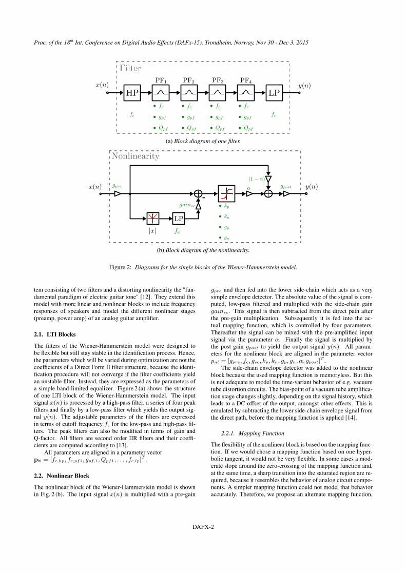
(a) Block diagram of one filter.

LP

(b) Block diagram of the nonlinearity.

Figure 2: Diagrams for the single blocks of the Wiener-Hammerstein model.

tem consisting of two filters and a distorting nonlinearity the "fun-damental paradigm of electric guitar tone" [12]. They extend thismodel with more linear and nonlinear blocks to include frequencyresponses of speakers and model the different nonlinear stages(preamp, power amp) of an analog guitar amplifier.

2.1. LTI Blocks

The filters of the Wiener-Hammerstein model were designed tobe flexible but still stay stable in the identification process. Hence,the parameters which will be varied during optimization are not thecoefficients of a Direct Form II filter structure, because the identi-fication procedure will not converge if the filter coefficients yieldan unstable filter. Instead, they are expressed as the parameters ofa simple band-limited equalizer. Figure 2 (a) shows the structureof one LTI block of the Wiener-Hammerstein model. The inputsignal x(n) is processed by a high-pass filter, a series of four peakfilters and finally by a low-pass filter which yields the output sig-nal y(n). The adjustable parameters of the filters are expressedin terms of cutoff frequency fc for the low-pass and high-pass fil-ters. The peak filters can also be modified in terms of gain andQ-factor. All filters are second order IIR filters and their coeffi-cients are computed according to [13].

All parameters are aligned in a parameter vectorplti = [fc,hp, fc,pf1, gpf,1, Qpf1, . . . , fc,lp]

T .

2.2. Nonlinear Block

The nonlinear block of the Wiener-Hammerstein model is shownin Fig. 2 (b). The input signal x(n) is multiplied with a pre-gain

gpre and then fed into the lower side-chain which acts as a verysimple envelope detector. The absolute value of the signal is com-puted, low-pass filtered and multiplied with the side-chain gaingainsc. This signal is then subtracted from the direct path afterthe pre-gain multiplication. Subsequently it is fed into the ac-tual mapping function, which is controlled by four parameters.Thereafter the signal can be mixed with the pre-amplified inputsignal via the parameter α. Finally the signal is multiplied bythe post-gain gpost to yield the output signal y(n). All param-eters for the nonlinear block are aligned in the parameter vectorpnl = [gpre, fc, gsc, kp, kn, gp, gn, α, gpost]

T .The side-chain envelope detector was added to the nonlinear

block because the used mapping function is memoryless. But thisis not adequate to model the time-variant behavior of e.g. vacuumtube distortion circuits. The bias-point of a vacuum tube amplifica-tion stage changes slightly, depending on the signal history, whichleads to a DC-offset of the output, amongst other effects. This isemulated by subtracting the lower side-chain envelope signal fromthe direct path, before the mapping function is applied [14].

2.2.1. Mapping Function

The flexibility of the nonlinear block is based on the mapping func-tion. If we would chose a mapping function based on one hyper-bolic tangent, it would not be very flexible. In some cases a mod-erate slope around the zero-crossing of the mapping function and,at the same time, a sharp transition into the saturated region are re-quired, because it resembles the behavior of analog circuit compo-nents. A simpler mapping function could not model that behavioraccurately. Therefore, we propose an alternate mapping function,

DAFX-2

Proc. of the 18th Int. Conference on Digital Audio Effects (DAFx-15), Trondheim, Norway, Nov 30 - Dec 3, 2015

consisting of three hyperbolic tangents which are concatenated atthe location denoted by kp for the positive part of input levels andat kn for the negative part. The tanh functions above or respec-tively below kp and kn are modified so that they have the sameslope as the middle part of the function at the connection points,shown in Eq. 1.

m(x) =

tanh(kp)−

[tanh(kp)

2−1

gptanh(gpx− kp)

]if x > kp

tanh(x) if − kn ≤ x ≤ kp−tanh(kn)−

[tanh(kn)2−1

gntanh(gnx+ kn)

]if x < −kn

(1)The parameters gp and gn control the smoothness of the transitionbetween saturated region and linear center part. For high values ofgp and gn the transition is very sharp, for low values it is smoothand for very small values and correctly chosen values of kx and kpit behaves like a linear function.

−1 −0.5 0 0.5 1−1

−0.5

0

0.5

1

Input Amplitude

Out

putA

mpl

itude

p1 = [0.5,0.5,0,0]p2 = [0.1,0.1,6,40]p3 = [0.1,0.25,15,40]p4 = [0.1,0.5,100,40]

Figure 3: Modified tanh function with the parametersp = [kp, kn, gp, gn]. Gain values for gp and gn are in dB.

Figure 3 illustrates the modified tanh function. The darkestcurve for parameter set p1 shows a nearly linear mapping functionwith relatively high values for kn > 0.5 and kp > 0.5 and lowvalues for gn < 1 dB and gp < 1 dB. For positive input ampli-tudes p2, p3 and p4 have steadily increasing gain values gp andthe same connection point kp = 0.1. This changes the shape ofthe nonlinear mapping function. The gain gn was kept constant atgn = 40 dB for negative input amplitudes, while the connectionparameter kn was shifted for p2, p3 and p4. Positive and negativesections of each curve could be interchanged by simply changingthe corresponding gain and connection parameters.

3. IDENTIFICATION

The concept of iterative error minimization is shown in Fig. 4. Thesame input signal is sent through the digital model and the refer-ence system, y(n) denotes the desired output from the DUT, whiley(p, n) denotes the model output, which is not only dependent onthe input samples, but also on a set of parameters p, which wereintroduced in Sec. 2. If the model is nonlinear for at least one

Figure 4: Block diagram of iterative error minimization.

parameter, it has to be identified iteratively [15]. The error signale(p, n) = y(n)− y(p, n) is calculated by subtracting the modeloutput from the reference output. The parameter estimation algo-rithm calculates a new set of parameters, which are applied to themodel in order to minimize the error between digital model andanalog system according to a cost-function C, in our case least-squares, C(p) =

∑Nn=1 e(p, n)

2. Where N is the length of theinput signal in samples. The parameter estimation method used inthis work is the Levenberg-Marquardt algorithm. This algorithmcombines the advantages of gradient-descent and Gauss-Newtonmethod [16, 17].

Before the identification procedure can be started, the refer-ence signals need to be recorded. For this purpose a high qualityaudio interface (RME Fireface UC TM) was used, which is con-trolled via Matlab. The DUT is placed between output and in-put of the audio interface. Before the actual input signals aresend through the DUT, the interface is calibrated by sending atest signal x(n) = sin

(2π f0

fsn)

with an amplitude of 0 dBFS,while the DUT is in bypass mode. The fundamental frequency isf0 = 1 kHz. The output gain of the interface was adjusted, so thatan amplitude of 1 corresponds to 1 V at the output of the audiointerface.

3.1. Nonlinear Identification

There are two different input signals for the identification of thelinear and nonlinear parts of the Wiener-Hammerstein model. Theinput signal,

xnl(n) = a(n) ·M∑i=1

sin(2π ·

[fi · sin

(2π

fmod,i

fsn

)]), (2)

for the identification of the nonlinear block is created by sum-ming several sine waves with different fundamental frequencies.Where a(n) is a scaling function, creating a logarithmically risingamplitude from −60 dBFS to 0 dBFS to emphasize lower signallevels. f = (50, 100, . . . , 900, 1000)Hz is a vector containingall the desired frequencies that roughly cover the range of notesthat can be played on a guitar and fmod,i is a vector containingthe modulation frequencies, which range from fmod,min = 1Hz tofmod,max = 10Hz and are used to avoid destructive and construc-tive interference which affect the envelope of the signal. M is theamount of sine waves which are summed and then normalized toachieve a maximum amplitude of 1.

When the parameters of a nonlinear model are optimized by aniterative error minimization algorithm, like the Levenberg-Marquardt

DAFX-3

Proc. of the 18th Int. Conference on Digital Audio Effects (DAFx-15), Trondheim, Norway, Nov 30 - Dec 3, 2015

method, it is very important to have an appropriate set of initial pa-rameters. The minimization algorithm might converge into a localminimum if the wrong set of initial parameters is chosen. Thus, ev-ery possible combination of the parameters gpre, kp, kn, gp and gnis tested on a coarse grid by calculating the sum of squares C(p)for each combination. The set with the lowest sum of squares isused as the initial parameter set for the identification process.

Because the parameters gpre, kp, kn, gp and gn have the mostinfluence on the envelope of the input signal, this procedure helpsfinding a starting point, which is most likely to converge into theglobal minimum of the cost function. During the iterative errorminimization, only the parameters of the parameter vector pnl areoptimized. The parameters of the two LTI blocks are fixed andcan not be changed during this identification step. The parametersin the plti vectors are set to yield a neutral filter characteristic inthe audible frequency range for both filters. After the optimizationpnl is saved for further use.

3.2. Filter Identification

The input signal for the parameter optimization of the LTI blocksis white noise with signal levels below −50 dBFS, because we as-sume, that for low signal levels the nonlinear part of the referencesystem operates in its linear region and tanh(x) ≈ x for |x| � 1is also true for the nonlinear block of the digital model.

In this case optimization of time domain error signals is chal-lenging because the signal can look different in time domain, dueto deviating phase characteristics of simulation and reference sys-tem, but is still perceived as similar for the human ear. For thisreason the output signals y(n) and y(p, n) need special treatmentbefore the actual minimization procedure can be started.

First the saved parameters from the identification of the non-linear block are loaded and used during filter parameter optimiza-tion. This helps identifying both filters of the model. If the filter’sparameters would be identified before the nonlinear parameters inthe first optimization step, characteristics of the first filter couldbe optimized onto the second filter and vice versa even though theoverall frequency response is retained.

The time domain output sequence for the white noise identifi-cation input is recorded. The power spectral density (PSD) of theoutput is computed by calculating a 16384-point discrete Fouriertransform (DFT) with a hop size of 4096 samples. All calculatedspectra are averaged and multiplied by its complex conjugate toyield the PSD. But the frequency resolution of a PSD or DFT re-spectively does not correspond to the perceptual resolution of thehuman ear. For this reason the semi-tone spectrum is calculatedfrom the PSD by averaging the frequency bins corresponding toone note. The first note is A0 in the sub contra octave which has afrequency of f0,A0 = 27.5Hz, which is one note below the lowestnote on a standard tuning 5-string bass. This is done for referenceand digital model respectively before the error signal is calculated.

The initial values for the identification procedure are chosenin such a way that the filter is flat and the cutoff frequencies ofhigh- and low-pass filters are set to fc,HP = 10Hz and fc,LP =18 kHz. After the filter parameters are adapted, they are stored forfurther use.

3.3. Overall Identification

In this final step the stored parameter vectors for both LTI blocksand the nonlinear block are loaded and used as the initial parameter

set in the final parameter vector

p =

plti1

plti2

pnl

. (3)

The Levenberg-Marquardt algorithm is started and now all pa-rameters of the model can be modified to refine the results fromthe previous optimization runs. The input signal for this step isthe same as for the optimization of the nonlinear parameters, de-scribed in Subsec. 3.1. The identification is not done solely in timedomain. This approach helps finding an initial parameter set forthe error minimization which is likely to converge into the globalminimum of the cost function. The spectrogram (8192-point DFT,4096 hop size) of the output of the analog system and the digitalsimulation is calculated and then vectorized as the minimizationalgorithm is not able to process error signals which are not in vec-torial form. By optimizing over the spectrogram error signal thenecessary information for adapting the filter and nonlinear param-eters is included.

4. RESULTS

As stated in Subsec. 3.2 it is challenging to find an objective er-ror measure for the perceived differences between to audio sig-nals. For this reason the error between simulation and reference isshown in time-domain as well as frequency-domain.

4.1. Time-Domain Error

A possible objective error measure would be the time domain error,

eyy =

∑Nn=1(y(n)− y(p, n))

2

N, (4)

whereN is the overall length in samples of the output signals. Theerror becomes zero if the signals are completely the same. But incertain cases, the time domain error is quite high but the perceived(subjective) difference is hard to hear. In general however, the timedomain error gives us an estimate about how close the model canrecreate the DUT. Nevertheless this is no reliable metric to charac-terize the perceptual difference between two audio signals. Figure5 shows the comparison between time domain signals of DUT andthe identified model. The DUT was a Hughes & Kettner - TubeFactor, which is basically a tube-preamp in stompbox format witha 12AX7 vacuum tube. Figure 5 (a) shows the response of digi-tal model and reference system to an exponentially decaying sineinput with 440Hz. The maximum amplitude of the input was 1.The digital model reproduces the analog system quite well, ex-cept from the transient part at the beginning of the signal. For therecorded electrical guitar signal, depicted in Fig. 5 (b), the simu-lation follows the measured curve closely but there are still somedifferences for certain frequency components, which may be a re-sult of the simple nonlinear block, where one nonlinear functionis used for all frequency components of the input signal. Anotherway of determining how well the identification worked, is by com-paring the transfer functions of both, reference and simulation.

4.2. Time and Frequency-Domain Error

Figure 6 shows the frequency response of a Jim Dunlop - FuzzFace fuzz pedal in comparison to the frequency response of its

DAFX-4

Proc. of the 18th Int. Conference on Digital Audio Effects (DAFx-15), Trondheim, Norway, Nov 30 - Dec 3, 2015

0.5 0.52 0.54−0.4

−0.2

0

0.2

0.4

t in s

Am

plitu

de

ReferenceSimulation

(a) 40ms 440Hz sin with exponentially decaying amplitude.

3.42 3.43 3.43−1

−0.5

0

0.5

1

t in s

Am

plitu

de

ReferenceSimulation

(b) Excerpt from recorded guitar signal.

Figure 5: Comparison of the time-domain signals for the Hughes& Kettner Tube Factor and the identified model.

102 103 104−40

−20

0

20

40

Frequency in Hz

Mag

nitu

dein

dB

SystemModel

Figure 6: Comparison of the frequency response of analog refer-ence and digital model for a Jim Dunlop - Fuzz Face.

digital model. The model deviates from the reference system byless than 1 dB, but becomes more inaccurate for low frequencies(below 60Hz) and for frequencies above 18 kHz.

The spectrograms of digital model and analog system outputare shown in Fig. 7. The input to both reference system and digi-tal model was a recording of an electrical guitar playing fast highchords, as customary for funk music. The DUT was a Hughes &Kettner - Tube Factor. The harmonics generated by the DUT andits digital representation resemble each other well. The error spec-trogram, shown in Fig. 7 (c), shows the difference of the absolutevalues of the previous spectrograms. The overall error energy ismuch lower than the signal energy of reference system and digitalmodel.

0 0.5 1 1.50

0.5

1

1.5

2

·104

Time in seconds

Freq

uenc

yin

Hz

(a) Reference

0 0.5 1 1.50

0.5

1

1.5

2

·104

Time in seconds

Freq

uenc

yin

Hz

(b) Simulation

0 0.5 1 1.50

0.5

1

1.5

2

·104

Time in seconds

Freq

uenc

yin

Hz

(c) Error

Figure 7: Spectrograms of reference system and digital model out-put and the error spectrogram.

4.3. Aliasing

The sampling frequency was set to fs = 48 kHz for identificationand runtime operations. The upper plot of Fig. 8 shows the fre-quency response of the digital model to a 1500Hz sine wave. Thealiasing, caused by the nonlinear block of the Wiener-Harmmersteinmodel is clearly visible due to the distinct peaks between the mainpeaks for fundamental frequency and the harmonics. For this rea-son resampling was introduced. The output signal of the first LTIblock is upsampled by resampling factor L, then processed by thenonlinear block and finally the output of the nonlinear block isdownsampled by factor L. The lower plot of Fig. 8 shows the re-sponse of the digital model to a 1500Hz sine wave with resam-pling factor L = 8. The effects of aliasing are now nearly dimin-ished.

DAFX-5

Proc. of the 18th Int. Conference on Digital Audio Effects (DAFx-15), Trondheim, Norway, Nov 30 - Dec 3, 2015

0 0.5 1 1.5 2

·104

−100

−80

−60

−40

−20

0

Frequency in Hz

Mag

nitu

dein

dB

0 0.5 1 1.5 2

·104

−100

−80

−60

−40

−20

0

Frequency in Hz

Mag

nitu

dein

dB

Figure 8: Response of the digital model to a 1500Hz sine. Above:without oversampling. Below: with 8 times oversampling.

4.4. Auditory Impression

Although no formal listening test was conducted, the subjectiveauditory impression of the proposed model is quite satisfying. Insome cases the difference between simulation and reference outputis still audible but only for a trained listener. Different input signalsas well as digital model and analog system outputs can be foundonline. Please visit [18] for listening examples.

5. CONCLUSIONS

This work proposed a method to identify and model nonlinear ana-log distortion effects. LTI filter blocks and a nonlinear block ofa Wiener-Hammerstein model, are introduced. The identificationroutine is described and the model is able to emulate any distor-tion pedal in a given setting. For many effects the results from themodel are nearly indistinguishable from the analog device itself.But this method still has several drawbacks, which should be ad-dressed in the future. First the search for the initial parameter setis still carried out on a coarse grid, because the computational ef-fort rises drastically if the grid resolution or the amount of testedparameters increases. This may cause the identification algorithmto converge into a local minimum instead of the global minimum.Furthermore it is essential to study more perceptually motivatederror metrics, e.g. PEAQ, to find a comparable and reliable errormetric.

6. REFERENCES

[1] D. Yeh, J.S. Abel, and J.O. Smith, “Automated physical mod-eling of nonlinear audio circuits for real-time audio effects:Part 1 - theoretical development,” in IEEE Trans. Audio,Speech, and Language Process., May 2010, vol. 18, pp. 203–206.

[2] D. Yeh and J.O. Smith, “Simulating guitar distortion circuitsusing wave digital and nonlinear state-space formulations,”

in Proc. Digital Audio Effects (DAFx-08), Espoo, Finland,Sept. 1-4, 2008, pp. 19–26.

[3] J. Macak, Real-time Digital Simulation of Guitar Amplifiersas Audio Effects, Ph.D. thesis, Brno University of Technol-ogy, 2011.

[4] K. Dempwolf, Modellierung analoger Gitarrenverstärkermit digitaler Signalverarbeitung, Ph.D. thesis, Helmut-Schmidt-Universität, 2012.

[5] M. Holters and U. Zölzer, “Physical modelling of a wah-wah effect pedal as a case study for application of the nodaldk method to circuits with variable parts,” in Proc. DigitalAudio Effects (DAFx-11), Paris, France, Sept. 19-23, 2011,pp. 31–35.

[6] A Novak, L. Simon, P. Lotton, and J. Gilbert, “Chebyshevmodel and synchronized swept sine method in nonlinear au-dio effect modeling,” in Proc. Digital Audio Effects (DAFx-10), Graz, Austria, Sept. 6-10, 2010.

[7] A. Novak, L. Simon, F. Kadlec, and P. Lotton, “Nonlinearsystem identification using exponential swept-sine signal,”Instrumentation and Measurement, IEEE Trans. on, vol. 59,no. 8, pp. 2220–2229, 2010.

[8] R. Cauduro Dias de Paiva, J. Pakarinen, and V. Välimäki,“Reduced-complexity modeling of high-order nonlinear au-dio systems using swept-sine and principal component anal-ysis,” in Audio Engineering Society Conference: 45th Inter-national Conference: Applications of Time-Frequency Pro-cessing in Audio, Mar 2012.

[9] A. Farina, “Simultaneous measurement of impulse responseand distortion with a swept-sine technique,” in Audio Engi-neering Society Convention 108, Paris, France, 2000.

[10] International Telecommunication Union, “Bs.1387: Methodfor objective measurements of perceived audio quality,”url, Available online at http://www.itu.int/rec/R-REC-BS.1387 − accessed June 1st 2015.

[11] C. Kemper, “Musical instrument with acoustic transducer,”US Patent: US20080134867 A1, July 2008.

[12] Fractal Audio Systems, “Multipoint Iterative Matching andImpedance Correction Tevhnology (MIMICTM),” Tech. Rep.,Fractal Audio Systems, April 2013.

[13] U. Zölzer, DAFx - Digital Audio Effects, John Wiley andSons, 2011.

[14] J. Pakarinen and D. T. Yeh, “A review of digital techniquesfor modeling vacuum-tube guitar amplifiers,” Computer Mu-sic Journal, vol. 33, no. 2, pp. 85–100, 2009.

[15] T. Strutz, Data fitting and uncertainty: a practical intro-duction to weighted least squares and beyond, Vieweg andTeubner, 2010.

[16] K. Levenberg, “A method for the solution of certain problemsin least squares,” Quarterly of applied mathematics, vol. 2,pp. 164–168, 1944.

[17] D. W. Marquardt, “An algorithm for least-squares estimationof nonlinear parameters,” Journal of the Society for Indus-trial & Applied Mathematics, vol. 11, no. 2, pp. 431–441,1963.

[18] “Listening Examples,” Website, Available at http://www2.hsu-hh.de/ant/webbox/audio/eichas/dafx15/audio_examples_local_version.html− accessed June 4th 2015.

DAFX-6