bivariate issues in leader election algorithms with marshall-olkin limit distribution

Methodol Comput Appl ProbabDOI 10.1007/s11009-014-9428-1

Bivariate Issues in Leader Election Algorithmswith Marshall-Olkin Limit Distribution

Cheng Zhang ·Hosam Mahmoud

Received: 13 May 2014 / Revised: 15 October 2014 / Accepted: 28 October 2014© Springer Science+Business Media New York 2014

Abstract Most prior work in leader election algorithms deals with univariate statistics. Weconsider multivariate issues in a broad class of fair leader election algorithms. We investi-gate the joint distribution of the duration of two competing candidates. Under rather mildconditions on the splitting protocol, we prove the convergence of the joint distribution of theduration of any two contestants to a limit via convergence of distance (to 0) in a metric spaceon distributions. We then show that the limiting distribution is a Marshall-Olkin bivariategeometric distribution. Under the classic binomial splitting we are able to say a few moreprecise words about the exact joint distribution and exact covariance, and to explore (viaRice’s integral method) the oscillatory behavior of the diminishing covariance. We discussseveral practical examples and present empirical observations on the rate of convergence ofthe covariance.

Keywords Randomized algorithm · Stochastic recurrence · Marshall-Olkin distribution ·Weak convergence · Rice’s integral method

Mathematics Subject Classification (2010) 60C05 · 60E05 · 68W40

1 Introduction

Lately, leader election algorithms have become a subject of intensive study, mainly becauseof their potential use in various applications. Many interesting parameters have been stud-ied in fair leader election, ranging from the duration of the algorithm till termination(see Fill et al. (1996) and Janson and Szpankowski (1997)), the total cost till termina-tion (Kalpathy and Mahmoud 2014; Prodinger 1993), to the number of rounds a contestantsurvives (Kalpathy and Mahmoud 2014; Kalpathy et al. 2011), and the number of survivorsafter a prespecified number of rounds (Kalpathy et al. 2013). All these investigations are

C. Zhang · H. Mahmoud (�)Department of Statistics, The George Washington University, Washington, DC 20052, USAe-mail: [email protected]

mailto:[email protected]

Methodol Comput Appl Probab

concerned with univariate statistics in leader election. In this note we address multivariateissues that can give us a more refined view of the overall random structure.

In the univariate setting, the classic example of binomial splitting has been thoroughlystudied (Fill et al. 1996; Janson and Szpankowski 1997; Janson et al. 2008; Kalpathy et al.2011; Louchard and Prodinger 2009; Louchard et al. 2011; Louchard et al. 2012). Onlyvery recently did research branch out of the specific case of binomial splitting to moregeneral splitting protocols. For instance, the reference (Kalpathy and Ward 2014) considerstruncated geometric distributions as splitting protocols, while Janson et al. (2008), Kalpathyand Mahmoud (2014), Kalpathy et al. (2013) consider broader theories that cover largeclasses of probability distributions.

In this article, we consider only fair leader election algorithms. In a fair leader electionalgorithm we restrict splitting algorithms to those in which a priori all participants haveequal chance of winning the contest. Such an algorithm is initialized with a number of con-testants competing fairly to elect a winner. In some variations the procedure may result inno winners at all, and all contestants lose. The contestants go through elimination roundsin which events are generated by contestants, agents or moderators. These events decidewhether or not they advance to the next round. Those who advance, compete again recur-sively till a winner is selected or the election is considered winnerless. Below, we shalldescribe more precisely the methods of recursive application on the advancing contestants.

As we mention in the preceding paragraphs, Kalpathy and Mahmoud (2014) looks at thedistribution of the duration of a particular individual contestant, a statistic that is importantfrom the vantage point of that individual contestant. In this note we look at the various layersat which contestants can fall and examine the covariance structure between the variousdurations. The joint distribution of two durations can tell one contestant how well otherswill do compared to him/herself. That is, this joint distribution specifies the prospect ofcompeting against other constants, which impacts settling bilateral scores and side betsbetween two contestants, and may influence budget planning, if there are entry fees or othercosts at each stage.

As the quest continues for broad theories, we examine joint distributions and the covariancestructure under a large class of splitting protocols that satisfy a set of mild regularity conditions.

The paper is structured in sections as follows. In Section 2 we describe the recursivealgorithms. The technical work is done in Section 3, which is divided into three subsec-tions: Section 3.1 sets up the basic two-dimensional stochastic recurrence, Section 3.2 iswhere proofs of convergence by the contraction method are, and in Section 3.3 we derivea Marshall-Olkin joint limiting distribution for the duration of pairs of participants. InSection 4, we thoroughly discuss the joint distribution under the specific binomial splittingprotocol in two subsections: Section 4.1 is for exact and limit distributions, and Section 4.2is where the oscillations are discussed. To put the results in perspective, the paper is con-cluded in Section 5 with some practical examples and empirical observations that help usdiscern rates of convergence under splitting protocols other than the binomial.

2 Leader Election

A priori, we have a predetermined sequence of random variables, K0, K1, K2, . . . , with Kj

having a distribution on the set {0, 1, . . . , j }. We call this sequence of distributions thesplitting protocol—whenever we need to generate winning candidates, say, when the contestsize becomes j , we use the distribution of Kj to generate a random number which is thenumber of contestants to advance.


Initially, there are n contestants. A certain number Kn ∈ {0, 1, . . . , n}, having the nth dis-tribution from the given list is generated. Then, Kn candidates are fairly selected to advanceto the second round and the rest of the contestants are eliminated. Fair selection means that,given Kn = k, all

(nk

)subsets of the initially present contestants are equally likely choices

to be competitors in the second round. The process continues in this fashion till one leaderis elected, or till all contestants are eliminated (resulting in no winner), and that is when theelection is stopped.

There is a one-sided tree structure underlying the process—all the n contestants initiallyreside in a root node. Losers of the first round are placed in a leaf node that appears as aright child of the root; which is not developed any further. Those who advance to competein the second round (if any) are placed in a node that appears as the left child of the root,which is then developed recursively till all contestants are eliminated, or one winner appearsby itself as a left child of its parent, and is not developed further. Thus, the duration of acontestant is the length of the path (counted in terms of edges) from the root to the node it isin at the termination time. That is, a contestant’s duration is its depth in the underlying tree.We shall interchangeably use the terms “duration” and “depth” to mean the same thing. Asthe tree leaves containing losers are not developed, many authors call this kind of tree an“incomplete tree.” Figure 1 shows an incomplete tree underlying the election of six partic-ipants, with leaves represened by rectangles, and nodes under development represented byovals. The competition ends after three rounds, with 5 winning the contest.

3 Joint Duration of a Random Pair of Contestants

Let Dn,j be the number of rounds (the duration) the j th contestant participated in the tour-nament by the termination time of the algorithm. The incomplete tree in Fig. 1 has D6,1 = 1and D6,5 = 3. This duration is also the depth of the contestant in the incomplete tree under-lying the algorithm. Specifying the number of rounds till termination of the election is a

Fig. 1 Leader election choosinga winner from six contestants


description of the maximal duration of the entire algorithm (height of the tree). A descrip-tion of the different depths (levels of duration) can be of interest from a particular individualcontestant’s point of view.

Under a fair splitting policy, we have a symmetry principle—all contestants are equally

likely to be selected to advance, and for 1 ≤ i < j ≤ n, we have

(Dn,i

Dn,j

)=

(Dn,1

Dn,2

)

(hered= denotes equality in distribution). So, it is sufficient to develop results for

(Dn,1Dn,2

).

To simplify notation and economize in typography, let Xn = Dn,1, and Yn = Dn,2, to deal

with fewer subscripts. Thus,

(Xn

Yn

)also has the joint distribution of the duration of any two

specific contestants. Note also that it has the joint distribution of the duration of a randomlyselected pair of contestants.

3.1 A Stochastic Recurrence

We study the distribution of

(Xn

Yn

)by establishing a stochastic recurrence, which arises

from a trichotomy of cases:

(i) Contestants 1 and 2 both advance to the second round with probability (conditioned

on Kn) equal to

(n − 2Kn − 2

)

(n

Kn

) = Kn(Kn−1)n(n−1)

.

(ii) Contestant 1 advances to the second round while contestant 2 is immediately

eliminated, with conditional probability

(n − 2Kn − 1

)

(n

Kn

) = Kn(n−Kn)n(n−1)

. There is a sym-

metrical case where Contestant 2 advances to the second round while contestant 1 isimmediately eliminated; this event has the same probability by symmetry.

(iii) The two contestants 1 and 2 are both eliminated together and they do not advance

to the second round, which occurs with conditional probability

(n − 2Kn − 1

)

(n

Kn

) =

(n−Kn)(n−Kn−1)n(n−1)

.

Therefore, for n ≥ 2, and for a given Kn, we have a stochastic recurrence equation:

(Xn

Yn

)d=

⎧⎪⎪⎪⎪⎪⎪⎪⎪⎪⎪⎪⎨

⎪⎪⎪⎪⎪⎪⎪⎪⎪⎪⎪⎩

(XKn + 1YKn + 1

), with probability Kn(Kn−1)

n(n−1)

(XKn + 11

), with probability Kn(n−Kn)

n(n−1);

(1YKn + 1

), with probability Kn(n−Kn)

n(n−1);

(11

), with probability (n−Kn)(n−Kn−1)

n(n−1).


The initial conditions are

(X0

Y0

)=

(X1

Y1

)=

(00

).

To write these conditional recurrences in one distributional equation, we need an auxil-iary random variable uniformly distributed on (0, 1) defined on the same space as Kn. Wecall this continuous random variable U . In what follows we use the indicator notation 1E ,which assumes the value 1, if the event E occurs, and assumes the value 0, otherwise. Forn ≥ 2, we can concisely write the recurrence in the form

(Xn

Yn

)d= 1{

U<Kn(Kn−1)

n(n−1)

}(

XKn

YKn

)+ 1{

Kn(Kn−1)n(n−1)

<U<Knn

}(

XKn

0

)

+1{Knn <U<

Kn(2n−Kn−1)n(n−1)

}(

0YKn

)+

(11

)

= An

(XKn

YKn

)+

(11

), (1)

where

An =⎛

⎝1{

U<Kn(Kn−1)

n(n−1)

} + 1{Kn(Kn−1)

n(n−1)<U<

Knn

} 0

0 1{U<

Kn(Kn−1)n(n−1)

} + 1{Knn

<U<Kn(2n−Kn−1)

n(n−1)

}

⎞

⎠ ,

and Kn,U ,

(Xi

Yi

)are independent, for all i < n.

3.2 Contraction

We shall consider classes of splitting protocols satisfying Kn

n

L1−→ K, thus Kn grows indef-

initely in probability. Under this condition, if

(Xn

Yn

)converges in distribution, so would

(XKn

YKn

). The recurrence then suggests that

(Xn

Yn

)converges to a limiting random vector

(X

Y

)that satisfies the distributional equation

(X

Y

)d=

(1{U<K2} + 1{K2<U<K} 0

0 1{U<K2} + 1{K<U<K(2−K)}

)(X

Y

)+

(11

),

with

(X

Y

), U and K being independent.

We prove this guessed limit by applying a multivariate contraction method (Neininger2001). The idea of the method is to first show convergence to 0 of the distance betweenthe distribution of the bivariate vector and a limit under a suitable metric. The limitsatisfies a distributional equation, with the right-hand side being a contraction. Finally,Banach’s fixed-point theorem asserts the existence of a unique limiting distribution. Forthe reader’s convenience, we state the multivariate limit in Neininger (2001). The theo-rem uses the notation ||A||op := sup||x||=1 ||Ax|| for the spectral radius of a square matrixA (maximal eigenvalue), where ||.|| is the usual norm of a matrix. A suitable metric forthe task is Wasserstein’s second-order distance. Convergence in this metric is known toimply convergence in distribution, and in the first two moments. We shall us the symbolW2 to denotes the Wasserstein distance of order 2. The transpose of a matrix B will bedenoted by BT .


Theorem 3.1 (Neininger 2001) Let (Xn) be a sequence of d-dimensional square integrablemean 0 random vectors satisfying the distributional recursion

Xnd=

m∑

r=1

A(n)r X(n)

I(n)r

+ b(n), n ≥ n0,

where(

A(n)1 , . . . , A(n)

m , b(n), I(n))

,(

X(1)n

), . . . ,

(X(m)

n

)are independent, A(n)

1 , . . . , A(n)m

are square integrable random d × d matrices, b(n) is a square integrable random vector

with mean 0, X(r)n

d= Xn, and I(n) is a vector of random integers with I(n)r ∈ {0, . . . , n}, r =

1, . . . ,m;n ≥ 0. Assume the following conditions hold:

(i)(

A(n)1 , . . . , A(n)

m , b(n))

L1−→ (A∗

1, . . . , A∗m, b∗) , n → ∞,

(ii)m∑

r=1

E

[|| (A∗

r

)T A∗r ||op

]< 1,

(iii)

E

[1{I (n)

r ≤�}∪{I (n)r =n}||

(A(n)

r

)T

A(n)r ||op

]→ 0, n → ∞,

for all � ∈ N, r = 1, . . . ,m.

Then we have

W2(Xn, X) → 0, as n → ∞,

where X is the unique fixed point of the distributional equation

Xd=

m∑

r=1

A∗r X(r) + b∗,

with (A∗1, . . . , A(∗)

m , b∗), X(1), . . . , X(m) independent and X(r) d= X, ∀r = 1, . . . , m.

We appeal to Theorem 3.1 to prove the convergence of

(Xn

Yn

)satisfying the recur-

rence (1). Note that the model in Theorem 3.1 is centered. We shall apply the theoremwithout centering, since we can transform our model into a centered one and the centeringwill not affect the conditions, and only shifts the limit.

Theorem 3.2 Suppose we run a fair leader election algorithm with Kn being the splitting

protocol. Suppose Kn

n

L1−→ K, where K is supported over [0, 1] with mean E[K] < 1. Then(

Xn

Yn

)d−→

(X

Y

),

where

(X

Y

)is the unique fixed point of the distributional equation

(X

Y

)d= A∗

(X

Y

)+

(11

),


with

(X

Y

), U and K being independent, and

A∗ =(

1{U<K2} + 1{K2<U<K} 00 1{U<K2} + 1{K<U<K(2−K)}

).

Proof The recurrence (1) is a special case of a class of multivariate stochastic recurrencesin Theorem 3.1. Specializing the parameters in Theorem 3.1 to our case, we see that

m = 1; b(n) = b∗ =(

11

); I

(n)1 = Kn; Kn ∈ {0, 1, . . . , n},

and

A(n) =⎛

⎝1{

U<Kn(Kn−1)

n(n−1)

} + 1{Kn(Kn−1)

n(n−1) <U<Knn

} 0

0 1{U<

Kn(Kn−1)n(n−1)

} + 1{Knn <U<


}

⎞

⎠ .

We next check the conditions of Theorem 3.1:

(i) The matrix E[(A(n) − A∗)2] is a diagonal matrix with the top left element being

E

[(1{

U<Kn(Kn−1)

n(n−1)

} + 1{Kn(Kn−1)

n(n−1)<U<

Knn

} − 1{U<K2} − 1{K2<U<K})2

]

,

and the bottom right element being

E

[(1{

U<Kn(Kn−1)

n(n−1)

} + 1{Knn <U<


}− 1{U<K2}− 1{K<U<K(2−K)})2

]

.

A calculation ensues—the top left element reduces to

E

[(1{

U<Knn

} − ‘1{U<K})2

]

= E

[1{

U<Knn

} + 1{U<K} − 21{U<

Knn

}∩{U<K}

]

= E

[Kn

n

]+ E[K] − 2E

[min

{Kn

n,K

}]

= (E[K] + o(1)) + E[K]− 2E

[min

{K + oL1(1),K

}]

= (2E[K] + o(1)) − (2E[K] + o(1))

→ 0.

Similarly, we have the convergence

E

[(1{

U<Kn(Kn−1)

n(n−1)

} + 1{Knn <U<


} − 1{U<K2} − 1{K<U<K(2−K)})2

]

→ 0.

It fololws that

E

[(A(n) − A∗)2

]→

(0 00 0

).


(ii) We have

E

[||(A∗)T A∗||op

]< E[1{U<K2}] + E[1{K2<U<K} + 1{K<U<K(2−K)}]

= E [K(2 − K)]

< 1;The last inequality follows from the fact that the function x(2 − x) reaches itsmaximum 1 at x = 1.

(iii) For any � ∈ N, and large n, we have

E

[1{Kn≤�}∪{Kn=n}||(A(n))T A(n)||op

]

≤ E[1{Kn≤�}∪{Kn=n} max

{1{U<

Kn(Kn−1)n(n−1)

} + 1{ Kn(Kn−1)n(n−1)

<U<Knn },

1{U<Kn(Kn−1)

n(n−1)} + 1{ Kn

n<U<


}

}].

We compute the expectation by conditioning on U , and get

E

[1{Kn≤�}∪{Kn=n} ||(A(n))T A(n)||op

]≤ E

[1{Kn≤�}

Kn(2n − Kn − 1)

n(n − 1)

].

Note that the function x(2n − x − 1) is increasing on [0, n]—in the presence of theindicator, the bound is maximized at �. We proceed with

E

[1{Kn≤�}∪{Kn=n}||(A(n))T A(n)||op

]≤ �

n

(2n − � − 1

n − 1

)→ 0, as n → ∞.

The conditions of Theorem 3.1 have been checked. As n → ∞, we have the convergence

W2

((X

Y

),

(Xn

Yn

))→ 0.

Consequently,

(Xn

Yn

)converges to

(X

Y

)in distribution and in the first two moments.

3.3 Marshall-Olkin Bivariate Geometric Limit

We shall recognize that the limiting bivariate moment generating function is that of aMarshall-Olkin bivariate geometric distribution. For the reader’s convenience, we say a fewwords on how such a bivariate geometric distribution arises, and provide some references.

A Marshall-Olkin bivariate geometric distribution is generated from independent iden-

tically distributed bivariate Bernoulli vectors

{(Ai

Bi

)}∞

i=1, that assume one of the four

values

(00

),

(01

),

(10

)and

(11

), with respective probabilities p00, p01, p10, and p11.

The vector(X

)Y , with X counting the number of attempts till success in the A compo-

nents (number of 0’s before the first 1 in the sequence A1, A2, . . .), and with Y counting thenumber of attempts till success in the B components (number of 0’s before the first 1 in thesequence B1, B2, . . .) is said to have a Marshall-Olkin bivariate geometric distribution with

parameters

(p00 p01p10 p11

). The original derivation of this and many other discrete bivariate


distributions appear in Marshall and Olkin (1985). Saralees (2008) provides an excellentsurvey. The distribution has a known bivariate moment generating function:

eu+v

1 − p00eu+v

(p11 + p01(p10 + p11)

1 − (p00 + p01)eu+ p10(p01 + p11)

1 − (p00 + p10)ev

).

Theorem 3.3 Suppose {Kn}∞n=0 is a given splitting protocol and we run a leader election

among n contestants, in which a fair selection of a subset of contestants of a random sizeKn advance to the next round, and the algorithm is applied recursively on that subset, tillone leader is elected or none. Suppose

Kn

n

L1−→ K,

and K has a distribution supported on [0, 1], with mean E[K∗] < 1. Let

(Xn

Yn

)be a vector

with two components representing the depths of the first two contestants. We then have

(Xn

Yn

)d−→

(X

Y

),

where

(X

Y

)has a Marshall-Olkin bivariate geometric distribution with parameters

(E[K2] E [K(1 − K)]

E [K(1 − K)] E[(1 − K)2

])

.

Proof Starting from the standard definition of a bivariate moment generating function, wewrite

φ(u, v) = E[euX+vY ]

= eu+v(E[euX+vY ]P(1{U<K2}) + E[euX]P(1{K2<U<K})

+ E[evY ]P(1{K<U<K(2−K)}) + E

[(1 − K)2

])

= eu+v(φ(u, v)E[K2] + E

[(1 − K)2

]

+ (ψ(u) + ψ(v))E [K(1 − K)]) ,

where ψ(w) = E[ewX] is the moment generating function of the limiting depth. Rearrang-ing the terms in the latter equation, we obtain an explicit form:

φ(u, v) = e(u+v)E

[(1 − K)2

] + E[K(1 − K)](ψ(u) + ψ(v))

1 − E[K2]e(u+v).


It is shown in Kalpathy and Mahmoud (2014) that X has a geometric distribution withparameter 1−E[K], i.e., ψ(w) = (1−E[K])ew/(1−E[K]ew). After we write the limitingbivariate generating function in the form

φ(u, v) = eu+v

1−E[K2]eu+v

(E

[(1 − K)2

] + E[K(1−K)]E[1−K]1−E[K]eu

+E[K(1−K)]E[1−K]1−E[K]ev

),

we see that

(Xn

Yn

)has a limiting Marshall-Olkin bivariate geometric distribution with

parameters

(E[K2] E[K(1 − K)]

E[K(1 − K)] E[(1 − K)2

])

.

Corollary 3.1

Cov[Xn, Yn] → Var[K](1 − E[K2])(1 − E[K])2

.

Proof Convergence in the Wasserstein metric implies convergence in the first twomoments. Thus, we have Cov[Xn, Yn] → Cov[X,Y ]. The limiting covariance can be com-puted from the explicit bivariate generating function established in the proof of Theorem3.3 by taking partial derivatives. Namely, we compute

Cov[X, Y ] = E[XY ] − E[X]E[Y ]= ∂2φ(u, v)

∂u∂v

∣∣∣u=v=0

−(

∂φ(u, v)

∂u

)

u=0

(∂φ(u, v)

∂v

)

v=0.

A mechanical procedure of calculating derivatives yield the result.

4 Binomial Splitting

In binomial splitting, the protocol is for the contestants to flip coins, producing Heads (suc-cess) with probability p, and producing Tails (failure) with probability q = 1 − p. Thosewho succeed advance to the next round; those who fail are eliminated. The competition con-tinues, so long as there are at least two competing candidates. This splitting protocol mayresult in no winners. In this model, the splitting protocol is a sequence of binomial distribu-

tions of a varying number of experiments, but fixed rate of success. That is, Knd= Bin(n, p).

The transparent structure of this particular protocol is amenable to exact calculation andrefined asymptotics including oscillations.

4.1 Exact and Limiting Distributions

Our general result applies to this instance, yielding

(Xn

Yn

)d−→

(X

Y

),


where

(X

Y

)is a Marshall-Olkin bivariate geometric distribution with parameters

(p2 pq

pq q2

), i.e., p0,0 = p2, p1,1 = q2, and both p0,1 and p1,0 are equal to pq . Asymp-

totics are, of course, a statement about infinite n. However, we are also able to say a fewmore precise words about what happens for finite n in this instance. For example, we get

the exact joint distribution of

(Xn

Yn

)and exact covariance, for each n.

Theorem 4.1 For n ≥ 2, and i, j ≥ 1, we have

P(Xn = i, Yn = j) =⎧⎨

⎩

qpi+j−2(q + p(1 − pj )n−2 − (1 − pj−1)n−2

), f or i < j ;

q2p2(i−1) + 2qp2i−1(1 − pi)n−2, f or i = j ;qpi+j−2

(q + p(1 − pi)n−2 − (1 − pi−1)n−2

)f or i > j.

Proof Let us first consider the case of equal depths:

(Xn

Yn

)=

(i

i

). In this case, either

both contestants 1 and 2 lose the election in i rounds, or one of these two contestants winsin i rounds and the other loses in i rounds (which necessitates that all other contestants havealready lost by the ith round). In the case they both lose in i rounds, they must both flipHeads i − 1 times in the first i − 1 rounds, then they both flip Tails in the ith round. Hence,we have

P(Xn = i, Yn = i) = (p2)i−1(q2) + 2(pi)(pi−1q)(1 − pi)n−2.

Consider next the case of unequal depths:

(Xn

Yn

)=

(i

j

), with i < j . In this case,

Contestant 1 is eliminated in i rounds, after flipping Heads in the first i − 1 in the rounds,and Tails in the ith round. However, Contestant 2 and at least one other contestant stayin the competition till depth j − 1. Subsequently, reaching depth j for Contestant 2 can

occur in one of two ways that partition the event

(Xn

Yn

)=

(i

j

)in two disjoint events.

At termination, Contestant 2 can be at depth j as a loser or as a sole winner. Let Li,j bethe event that Xn = i, and Contestant 2 loses the contest by getting eliminated in the j thround,. We then have

P(Li,j ) = (pi−1q)(pj−1q)(

1 − (1 − pj−1)n−2)

.

Let Wi,j be the event that Xn = i, and Contestant 2 wins the contest in the j th round, inwhich case at least one other contestant loses in the j rounds (or else the contest would haveended earlier). The event Wi,j occurs, if Contestant 2 flips j Heads, provided that none ofthe other contestant flips j Heads, while at least one of the other n−2 contestants (excludingContestant 1) flips j − 1 Heads (or else the first contest would have ended earlier). Thus,

P(Wi,j ) = (pi−1q)(pj)((1 − pj )n−2 − (1 − pj−1)n−2

).

It now follows that

P(Xn = i, Yn = j) = P(Li,j ) + P(Wi,j )

= qpi+j−2(q + p(1 − pj )n−2 − (1 − pj−1)

).

The argument for the case i > j is, of course, symmetrical.


Corollary 4.1 As n → ∞, the vector

(Xn

Yn

)converges in distribution to a vector

(X

Y

)

of independent geometric random variables, with parameter p each.

Proof It is shown in Kalpathy et al. (2011) that XnD−→ X, and X is geometrically

distributed with parameter p. Note that

limn→∞P(Xn = i, Yn = j) = q2pi+j−2 = P(X = i)P(Y = j).

The exact covariance can be found from the exact distribution. Its limiting value is, of

course, 0, since the two components of

(XKn

YKn

)are ultimately independent. However, a pre-

cise analysis reveals minute oscillations that eventually disappear. To simplify the followingpresentation, we use the notation

cp = (p4r+7 − 3p3r+5 + 4p2r+3 + p2r+4 − 4pr+2 − p3r+6 + 2pr+3

− q2p2r+3 + q2pr+1)/(pr+2 − 1)3.

Corollary 4.2

Cov[Xn, Yn] = 2

q

n−2∑

r=0

(−1)r(

n − 2

r

)cp − pr+1(pr+1 − 2)

pr+1 − 1

+ 2

q

n−1∑

j=1

(−1)j(

n − 1

j

)1

1 − pj+1

−⎛

⎝n−1∑

j=1

(−1)j(

n − 1

j

)1

1 − pj+1

⎞

⎠

2

.

Proof The exact joint distribution in Theorem 4.1 yields the exact first mixed moment, forn ≥ 2:

E[XnYn] =∑

1≤i,j<∞ijP(Xn = i, Yn = j)

=∑

1≤i<∞i2P(Xn = i, Yn = i) + 2

∑

1≤i<j<∞ijP(Xn = i, Yn = i).

This is a daunting computation. We only outline the main steps. We collect all the terms thatare dependent on i and j only (and not on n). The series so obtained is easily summed, giving1/q2. We then expand each of the terms raised to the power n − 2 in the joint probabilityby the binomial theorem, and interchange the order of summation to deal with the sums onr last. Combined, these parts give

2

q

n−2∑

r=0

(−1)r(

n − 2

r

)(

cp − pr+1((pr+1 − 2)

pr+1 − 1

)

=: An.


The lemma follows by writing

Cov[Xn, Yn] = 1

q2+ An − E[Xn]E[Yn] = 1

q2+ An − (E[Xn])2 .

The proof is completed by plugging in the average of Xn (given in Kalpathy et al. (2011)),which is

E[Xn] = 1

q−

n−1∑

j=0

(n − 1

j

)(−1)j

1 − pj+1.

4.2 Oscillations

Let

g(r) = cp − pr+1((pr+1 − 2)

pr+1 − 1.

To detect oscillations, we analyze the asymptotics in a more refined way, reaching lowerorder asymototics via an analytic method. Replace r by z ∈ C in g to get a continuationof g to a complex function in the complex plane. The continuation g(z) coincides with thevalue g(r) at each value in the domain of definition of r , and is analytic at all z ∈ C exceptat the poles of g(z).

The alternating signs and binomial coefficients in the sum An are a hallmark of Rice’sintegral method (Flajolet and Sedgewick 1995). The basic idea in that method is to recognizethat such an alternating sum is the same as

− 1

2πi

∮

C1

β(n − 1,−z)g(z)dz,

where β(., .) is the Beta function, and the line integral is taken over a “thin” closed contourC1 surrounding the integers 0, 1, . . . , n − 2 and no other. The contour C1 can be takenas the rectangle connecting the four corners at − 1

2 ± i and n − 1 ± i. The connectionbetween the sum and the line integral is that the integrand has simple poles at the integerpoints 0, 1, . . . , n − 2, with residues coinciding with the negative of the summands. Theintegral is then evaluated via the residues of the poles outside C1 and a small error. This isdone by deforming C1 into a larger contour C2(a,M), say a rectangle connecting the fourcorners at −a ± π(2M + 1)i and n ± π(2M + 1)i, for a > 2, and large positive integerM . The two integrals over C1 and C2(a,M) differ by the residues of the poles enclavedbetween the two contours. The poles outside C1 are located at zk = −1 + 2πki/ ln p, andat z′

k = −2 + 2πki/ ln p, for k = 0,±1,±2, . . . . Let M → ∞; the rectangle C2(a,M)

grows to encompass all the poles outside C1, and

− 1

2πi

∮

C1

β(n − 1,−z)g(z)dz = − 1

2πilim

M→∞

∮

C2(a,M)

β(n − 1,−z)g(z)dz

+∞∑

k=−∞Resz=zk

β(n − 1,−z)g(z)

+∞∑

k=−∞Resz=z′

k

β(n − 1,−z) g(z).


By Stirling’s approximation to the Gamma function, we have the residue calculation

Resz=zk

g(z) = − 2 �(n − 1) �(−zk)

q �(n − 1 − zk) ln p= −2n−1+2πki/ ln p

q ln p�

(1 − 2πki

ln p

)(1 + O

(1

n

)),

and

Resz=z′

k

g(z) = O(n− 3

2

).

It can be shown that, as M → ∞, the contribution of the limiting contourlimM→∞ C2(a,M) is O(n−a).

Putting all the elements together, we get

E[XnYn] = 1

q2−

(2

q ln p

∞∑

k=−∞�

(1 − 2πik

ln p

)e2πik log1/p n

)1

n+ O

(1

n32

).

For (E[Xn])2, we use an asymptotic estimate from Kalpathy et al. (2011), and obtain

Cov[Xn, Yn] = 1

q2−

(2

q ln p

∞∑

k=−∞�

(1 − 2πik

ln p

)e2πik log1/p n

)1

n+ O

(1

n32

)

−(

1

q+

(1

ln p

∞∑

k=−∞�

(1 − 2πik

ln p

)e2πik log1/p n

)1

n+ O

(1

n2

))2

= − 4

q ln p

⎛

⎜⎝1 +

∞∑

k=−∞k �=0

�

(1 − 2πik

ln p

)e2πik log1/p n

⎞

⎟⎠

1

n+ O

(1

n2

)

→ 0.

The asymptotic equivalent of the covariance is diminishing and contains the oscillat-ing functions e2πik log1/p n. Collectively, the sum of all the oscillations is very small. Forinstance, in the unbiased case p = q = 1

2 , the sum is bounded absolutely by 5.7 × 10−5.

5 Practical Issues

We presented theoretical results for the covariance structure in leader election algorithms,when the splitting protocol produces a sequence of random variables that converges (uponappropriate scaling) in L1 to a limit. In practice, the rate of convergence may be of interestas well. A practitioner or a political campaign advisor may need to know how large n, thenumber of contestants, should be before he/she can accept the covariance limiting value asa reliable approximation.

We explored this issue theoretically under the binomial splitting. However, we do nothave a general theoretical result for the rate of convergence, and it may be hard to findthe rate of convergence of the covariance in closed form under other splitting protocols. Inthis section we explore the rate of convergence via simulation under two splitting protocolsother than binomial: uniform splitting and ladder splitting.

The reason for choosing these two particular splitting protocols stems from practi-cal considerations. We are more interested in protocols arising from a natural procedure


or a mechanical process, such as coin flips, picking labelled chips from a jar, computergeneration of random numbers, organization of sports tournaments, etc.

For instance, while a limiting beta (a, b) qualifies in the class of limits we studied, it maybe hard to achieve a beta (a, b) limiting random variable by a practicable process, whereasbinomial, uniform and ladder splitting correspond to rather natural processes that employvery simple functions and mechanical steps. That is, the latter three distributions arise morenaturally in many contexts. To better illustrate this point, we include the pseudocode for theleader election algorithms under the splitting protocols under discussion.

Take for instance the binomial splitting, which receives p and the set of candidates C asinput. The pseudocode for a binomial splitting leader election algorithm might look like:

n ← Size (C);while n > 1 do

n ← Bin(n, p);C ← Subset(C,n);

print (C);

This procedure assumes only primitive functions, like Size, one that measures the size ofa given set, and the algorithm assumes the presence of random number and set generators toproduce a binomially distributed random variable and a uniformly chosen subset of a givensize from a larger set (we refer to the Subset function used in the procedure). Many modernsystems like R provide such facility. We analyzed the rate of convergence of the covariancetheoretically and found a rate of O(1/n) convergence, with oscillations within.

The pseudocode for uniform splitting is similar, with a uniform random number generatorreplacing the line following the while loop in the previous code. Under this fair splittingprotocol, Kn = Un, with Un being a discrete random variable distributed uniformly onthe set {1, . . . , n}. So, on a suitable probability space, we have Kn/n = 1

2 + O(1/n).By Corollary 3.1, in this case the covariance between two randomly chosen participantsconverges to 1

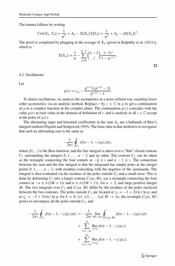
2 .We conducted simulations in R to observe how the covariance varies with the num-

ber of contestants n under a uniform splitting protocol. For each n ∈ {3, 4, . . . , 102},we obtained 10000 observations. The results of these simulations are shown in Fig. 2. Inthis figure, the horizontal axis represents the number of contestants, and the vertical axisrepresents the absolute value of the difference of the covariance between two contestantsand one half. It empirically appears that the rate of convergence is 1/n, possibly withfluctuations.

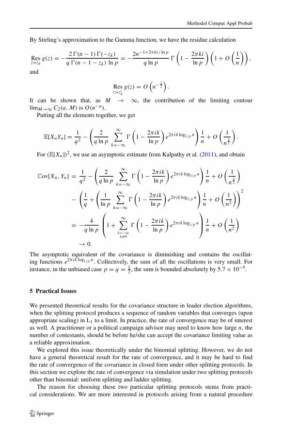
We can also describe a mechanical process associated with ladder splitting. Many real-life tournaments, such as the ones used in organizing major sports events like Wimbledon,the World Cup and NCAA March Madness are organized in ladders. In these contests, n

is usually a power of 2. We describe the ladder splitting protocol for arbitrary n. Given n

contestants, if n is even, we randomly group the contestants into n2 matches, and within each

matched pair we select the winner at random. If n is odd, we first select a “wildcard” atrandom, who advances (gets by) to the next round automatically. That is why the wildcardis often called a bye. Among the remaining n − 1 contestants, a pairing procedure similarto the one used for even n is applied to advance half of these n − 1 contestants. Note thatfairness is guaranteed by the randomization of the wildcard and by randomly advancingone contestant from each paired match. Among those who advance, we apply the sameprocedure recursively. Unlike the uniform splitting protocol, a ladder guarantees selecting


Fig. 2 A plot of the absolute value of the difference between the covariance and 12 under a uniform splitting

protocol versus the number of contestants

a winner at termination. Receiving the set of candidates C as input, the pseudocode for aladder-based leader election might look like this:

n ← Size (C);while n > 1 do

randomize (order of C);if n mod 2 ≡ 1 then

wildcard ← C[n];NewC ← {wildcard}

else NewC ← ∅;for i ← 1 to �n

2 � doU ← uniform(0,1);if U < 1

2 then NewC ← NewC + {C[2i − 1]};else NewC ← NewC + {C[2i]};

C ← NewC;n ← Size (C);

print (C);


Fig. 3 A plot of the absolute value of the covariance under a ladder splitting protocol versus the number ofcontestants

In a fair ladder, Kn = � 12n�, and so Kn/n = 1

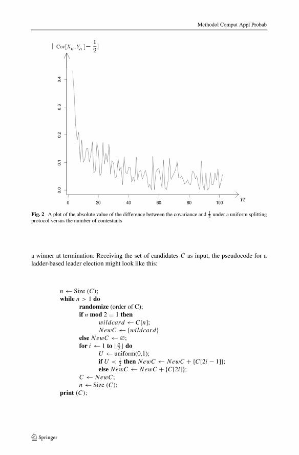
2 + O(1/n). It is easy to check that allthe conditions of Theorem 3.3. By Corollary 3.1, we see that the covariance converges to 0under a ladder splitting protocol.

We conducted simulations in R to observe how the covariance varies with the number ofcontestants n under a ladder splitting protocol. For each n ∈ {3, 4, . . . , 102}, we obtained10000 observations. The results of these simulations are shown in Fig. 3. In this figure, thehorizontal axis represents the number of contestants, and the vertical axis represents theabsolute value of the covariance between two contestants. It empirically appears that therate of convergence is 1/n, possibly with fluctuations.

Remark 5.1 By inspecting Corollary 3.1, we see that, among these practicable algorithms,the only facet of the splitting protocol that enters the picture in the limit is the first twomoments of the limiting variable K. All splitting protocols with a limiting K (satisfy-ing the conditions) with the same mean and variance have the same covariance structure.For instance, all splitting protocols where Kn converges to a constant (0 variance) willhave 0 covariance (and 0 correlation). The uniform example shows that practicable split-ting protocols can produce limiting covariances other than 0 (it is 1

2 in the uniformsplitting case).


Acknowledgment The authors would like to thank Dr. Winfried Barta for suggesting this problem ina local seminar. They also acknowledge the encouragement and critique provided by the referees, whichimproved the exposition.

References

Fill J, Mahmoud H, Szpankowski W (1996) The distribution for the duration of a randomized leader electionalgorithm. Ann Appl Probab 6:1260–1283

Flajolet P, Sedgewick R (1995) Mellin transforms and asymptotics: Finite differences and Rice’s integrals.Theor Comput Sci 144:101–124

Janson S, Szpankowski W (1997) Analysis of an asymmetric leader election algorithm. Electron J Comb4(R17):1–16

Janson S, Lavault C, Louchard G (2008) Convergence of some leader election algorithms. Discret MathTheor Comput Sci 10:171–196

Kalpathy R, Mahmoud H (2014) Perpetuities in fair leader election algorithms. Adv App Prob 46Kalpathy R, Ward M (2014) On a leader election algorithm: Truncated geometric case study. Stat Probab

Lett 87:40–47Kalpathy R, Mahmoud H, Rosenkrantz W (2013) Survivors in Leader Election Algorithms. Stat Probab Lett

83:2743–2749Kalpathy R, Mahmoud H, Ward M (2011) Asymptotic properties of a leader election algorithm. J Appl

Probab 48:569–575Louchard G, Prodinger H (2009) The asymmetric leader election algorithm: Another approach. Ann of Comb

12:449–478Louchard G, Martı́nez C, Prodinger H (2011) The Swedish leader election protocol: Analysis and varia-

tions. In: Flajolet P, Panario D (eds) Proceedings of the Eighth ACM-SIAM Workshop on AnalyticAlgorithmics and Combinatorics (ANALCO) San Francisco, pp. 127–134

Louchard G, Prodinger H, Ward M (2012) Number of survivors in the presence of a demon. Period MathHung 64:101–117

Marshall A, Olkin I (1985) A family of bivariate distributions generated by the Bernoulli distribution. J PublAm Stat Assoc 80:332–338

Neininger R (2001) On a multivariate contraction method for random recursive structures with applicationsto Quicksort. Random Struct Algorithm 19:498–524

Prodinger H (1993) How to select a loser. Discret Math 120:149–159Saralees N (2008) Marshall and Olkin’s Distributions. Acta Applicandae Math 103:87–100

bivariate issues in leader election algorithms with marshall-olkin limit distribution

Documents