NBER WORKING PAPER SERIES

BIRTHPLACE DIVERSITY AND ECONOMIC PROSPERITY

Alberto AlesinaJohann HarnossHillel Rapoport

Working Paper 18699http://www.nber.org/papers/w18699

NATIONAL BUREAU OF ECONOMIC RESEARCH1050 Massachusetts Avenue

Cambridge, MA 02138January 2013

We thank Amandine Aubry, Simone Bertoli, François Bourguignon, Frédéric Docquier, Jesús Fernández-HuertasMoraga, Oded Galor, Frédéric Jouneau, Thierry Mayer, Yona Rubinstein, Joao Santos-Silva, JacquesSilber, Sylvana Tenreyro, Nico Voigtlaender, participants at the 5th AFD-World Bank Conferenceon Migration and Development, Paris, June 2012, the 1st CEMIR conference at CESifo, Munich, December2012, the NBER Economics of Culture and Institutions Meeting, Cambridge, April 2013, the 10thIZA Migration Meeting in Jerusalem, June 2013, and seminar audiences at PSE-SciencePo-Paris 1(Paris Trade Seminar), Louvain (IRES), the Geneva Graduate Institute, Luxembourg, Milan, HebrewUniversity, Tel-Aviv, EUI and IDC for comments and suggestions. We also thank Quamrul Ashrafand Frédéric Docquier for sharing their datasets with us. The views expressed herein are those of theauthors and do not necessarily reflect the views of the National Bureau of Economic Research.

NBER working papers are circulated for discussion and comment purposes. They have not been peer-reviewed or been subject to the review by the NBER Board of Directors that accompanies officialNBER publications.

© 2013 by Alberto Alesina, Johann Harnoss, and Hillel Rapoport. All rights reserved. Short sectionsof text, not to exceed two paragraphs, may be quoted without explicit permission provided that fullcredit, including © notice, is given to the source.

Birthplace Diversity and Economic ProsperityAlberto Alesina, Johann Harnoss, and Hillel RapoportNBER Working Paper No. 18699January 2013, Revised August 2015JEL No. F22,F43,O1,O4

ABSTRACT

We use recent immigration data from 195 countries and propose an index of population diversity basedon people's birthplaces. This new index is then decomposed into a size (share of foreign born) anda variety (diversity of immigrants) component and is available for 1990 and 2000 disaggregated byskill level. We show that birthplace diversity is largely uncorrelated with ethnic, linguistic, or geneticdiversity. Our main result is that the diversity of skilled immigration relates positively to economicdevelopment (as measured by income and TFP per capita and patent intensity) even after controllingfor ethno-linguistic and genetic fractionalization, geography, trade, education, institutions and origin-effectscapturing income/productivity levels in the immigrants' home countries. We make progress towardsaddressing endogeneity by specifying a gravity model to predict the share and diversity of immigrationbased on exogenous bilateral variables. The results are robust across various OLS and 2SLS specificationsand suggestive of skill complementarities between native workers and immigrants, especially whenthe latter come from richer countries at intermediate levels of cultural proximity.

Alberto AlesinaDepartment of EconomicsHarvard UniversityLittauer Center 210Cambridge, MA 02138and IGIERand also NBERaalesina@harvard.edu

Johann HarnossEQUIPPE,University of Lille, and Harvard Universityjohann.harnoss@post.harvard.edu

Hillel RapoportDepartment of EconomicsBar Ilan University52900 Ramat Gan, Israeland QUIPPE, University of Lilleand also Center for International Development Hillel.Rapoport@biu.ac.il

1 Introduction

Population heterogeneity is increasing in virtually all advanced economies due to immigra-

tion. Foreign-born individuals now represent about ten percent of the workforce in OECD

countries, a threefold increase since 1960 and a twofold increase since 1990. High-skill mi-

gration is growing even faster, with a twofold increase during the 1990s alone.1 As a result,

the diversity of the skilled workforce (measured as the likelihood that two randomly-drawn

skilled workers have different countries of birth) in a typical OECD country has increased

by more than three percentage points (from .19 to .22) within just ten years.2

What are the economic implications of such higher diversity? Theory suggests that di-

versity has positive and negative economic effects. The former are due to complementarities

in production, diversity of skills, experiences and ideas (think of a Dixit Stiglitz production

function). The latter arise from potential conflicts, disagreements about public policies, and

animosity between different groups. A vast literature has investigated these issues. The

empirical literature has so far focused on ethnic and linguistic fractionalization, which were

shown to exert negative effects on economic growth in cross-country comparisons (Easterly

and Levine, 1997, Collier, 2001, Alesina et al., 2003, 2012), with the possible exception

of very rich countries (see Alesina and La Ferrara, 2005, for a discussion of these issues).

Ashraf and Galor (2013a,b) focus on genetic diversity and show that it exhibits an inverse

u-shaped relationship with income per capita. On balance the negative effects of diversity

seem to dominate empirically, or to put it differently, it has been hard to document the

positive economic effects of diversity. This is the key objective of this paper.

We examine the relationship between intrapopulation diversity in birthplaces and eco-

nomic prosperity. More specifically, we make four contributions. First, we construct and

discuss the properties of a new index of birthplace diversity. We build indicators of diver-

sity for the workforce of 195 countries in 1990 and 2000, disaggregated by skill/education

level, and computed both for the workforce as a whole and for its foreign-born component.

Empirically, ethno-linguistic and birthplace diversity are - somewhat surprisingly - almost

completely uncorrelated. Conceptually, ethnic, genetic and birthplace diversity also differ

as people born in different countries are likely to have been educated in different school sys-

tems, learned different skills, and developed different cognitive abilities. That may not be

the case for people of different ethnic origins born, raised and educated in the same country.

1See Ozden et al. (2011) for a picture of the evolution of international migration over the last fifty years,

and Docquier and Rapoport (2012) for a focus on high-skill migration and its effects on source and host

countries.2That is, a 17-percent increase. 22 out of 27 OECD countries saw increases in the diversity of their

skilled workforce between 1990 and 2000 (the only exceptions being Estonia, Greece, New Zealand, Poland

and Slovakia).

2

Second, we investigate the relationship between birthplace diversity and economic devel-

opment. We find that unlike ethnic/linguistic fractionalization, birthplace diversity remains

positively related to long-run income after controlling for many covariates. This positive rela-

tionship is stronger for skilled migrants (workers with college education) in richer countries.

In terms of magnitudes, increasing the diversity of skilled immigrants by one percentage

point raises long-run output by about two percent.

Third, we make progress towards addressing endogeneity issues arising from selection

on unobservables and reverse causality. We show that our results are unlikely to be ex-

plained by positive selection on unobservables. To address reverse causality, we specify

a gravity model to predict the size and diversity of a country’s immigration using bilat-

eral geographic/cultural variables. We confirm the robustness of our OLS findings in 2SLS

models.

Fourth, we allow the effect of diversity to vary with bilateral distance between immigrants

and natives along two dimensions: genetic/cultural distance, and income at origin. The

productive effect of birthplace diversity is largest for immigrants from richer origin countries

and for immigrants from countries at intermediate levels of cultural proximity. That is, the

effect of diversity is inversely u-shaped in terms of cultural distance between immigrant and

native workers. This suggests an optimal level of birthplace diversity in terms of cultural

proximity.3

The current empirical evidence linking income and productivity differences to birthplace

diversity is growing rapidly but is still limited when it comes to cross-country evidence.

Existing studies have focused mainly on the United States. Ottaviano and Peri (2006)

construct a measure of cultural diversity for the period 1970-1990 using migration data on

US metropolitan areas and find positive effects on the productivity of native workers as

measured by their wages.4 Peri (2012) finds positive effects of the diversity coming from

immigration on the productivity of US states, a result he attributes to unskilled migrants

promoting effi cient task-specialization and adoption of unskilled-effi cient technologies, and

more so when immigration is diverse. Ager and Brückner (2013) study the link between

immigration, diversity and economic growth in the context of the United States about a

century ago, at a time now commonly referred to as "the age of mass migration" (Hatton

and Williamson, 1998).5 They find that fractionalization increases output while polarization

decreases it in US counties during the period 1870-1920. Cross-country comparisons include

3This inverted u-curve for cultural proximity mirrors the results of Ashraf and Galor (2013a) on genetic

diversity.4Bellini et al. (2013) apply the same methodology to European regions and find broadly consistent results

for Europe as well.5See also Bandiera, Rasul and Viarengo (2013) and Abramitzky, Boustan and Eriksson (2012, 2013),

respectively, on the measurement of entry and return flows and on migrants’self-selection.

3

Andersen and Dalgaard (2011), who find positive effects of travel intensity on total factor

productivity which they attribute to knowledge diffusion of temporary migrants, and Ortega

and Peri (2014), who analyze the connection between income per capita and migration in a

cross-section of countries. They focus on the growth effects of openness and diversity of trade

vs. migration and find the share of immigration to be a stronger determinant of long run

output than trade. In contrast, we focus on the effect of intrapopulation diversity, comparing

birthplace to other dimensions of diversity (ethnic, linguistic, genetic) and demonstrate the

positive effect of the diversity arising from immigration (especially its high-skill component)

on income per capita.

The rest of this paper proceeds as follows. Section 2 briefly discusses theoretical chan-

nels and related literature on diversity and economic performance. Section 3 explains the

construction and analytical decomposition of our birthplace diversity index; we also explore

its descriptive features and patterns of correlation with other diversity/fractionalization in-

dices. In Section 4 we provide data sources, develop our empirical model, and describe OLS

results for birthplace diversity in a range of empirical specifications. In Section 5, we discuss

unobserved heterogeneity and reverse causality, showing that they are unlikely to explain

our results. In Section 6, we augment our birthplace diversity index to include bilateral

economic and cultural group distance between the native population and each immigrant

group. Section 7 concludes.

2 The literature

People born in different countries are likely to have different productive skills because they

have been exposed to different life experiences, different school and value systems, and thus

have developed different perspectives that allow them to interpret and solve problems differ-

ently. We use the term "birthplace diversity" to designate the dimension of intrapopulation

diversity arising from the heterogeneity in people’s birthplaces and posit that this source of

diversity is more likely to capture skill complementarity effects than alternative dimensions

of diversity (e.g., ethnic or linguistic fractionalization). Alesina et al. (2000) formalize the

idea of skill complementarities using a Dixit-Stiglitz type production function where output

increases in the variety of inputs and inputs can be interpreted as different type of work-

ers. Their model thus allows for diversity to increase output without any counterbalancing

costs. Lazear (1999a,b) proposes a model of teams of workers where diversity brings bene-

fits via production complementarities from relevant disjoint information sets and also costs

via barriers to communication; with decreasing marginal benefits and increasing marginal

costs, this suggests that there is an optimal degree of diversity. A related argument, also

brought forward by Lazear (1999b), is that diverse groups of immigrants tend to assimilate

4

more quickly (in terms of learning the language of the majority) since they have stronger

incentives to do so. Hong and Page (2001) see two sources for the heterogeneity of people’s

minds: cognitive differences between people’s internal perspectives (their interpretation of

a complex problem) as well as their heuristics (their algorithms to solve these problems).

They show theoretically that, under certain conditions, a group of cognitively diverse but

skill-limited workers can outperform a homogenous group of highly skilled workers. Fer-

shtman, Hvide and Weiss (2006) reach similar conclusions in a model where workers are

heterogeneous in terms of status concerns.6

Empirically, diversity is commonly measured by ethno-linguistic fractionalization (East-

erly and Levine 1997, Alesina et al., 2003, Fearon, 2003, Desmet et al., 2012) and ethno-

linguistic polarization indices (Esteban and Ray, 1994, Reynal-Querol, 2002 and Montalvo

and Reynal-Querol, 2005). At a macro level, the costs of fractionalization have been es-

tablished empirically in particular for ethno-linguistic diversity. These studies began with

Easterly and Levine (1997), who show that ethnic fragmentation is associated with lower

economic growth, especially in Africa. Collier (1999, 2001) adds that ethnic fractionalization

is less detrimental in the presence of democratic institutions that mediate ethnic conflict,

It is, however, unclear if this observation is not a corollary of higher income as shown in

Alesina and La Ferrara (2005). Fearon and Laitin (2003) add that ethnic diversity alone

is not suffi cient to explain the outbreak of civil war. Putnam (1995), and Alesina and La

Ferrara (2000, 2002) stress the role of trust, showing that individuals in racially diverse

cities in the US participate less frequently in social activities and trust their neighbors to a

lesser degree. The authors also find evidence that preferences for redistribution are lower in

racially diverse communities. This also extends to the provision of productive public goods

(Alesina, Baqir and Easterly, 1999). Alesina and Zhuravskaya (2011) stress the negative

effect of ethnic segregation on the quality of government, while Alesina, Michalopoulos and

Papaioannou (2015) highlight the detrimental effects of "ethnic inequality" (i.e., when eco-

nomic inequality and ethnic diversity go hand-in-hand). Esteban, Mayoral and Ray (2012)

distinguish conflicts over public and private goods and find polarization to correlate posi-

tively with conflict on the former, and fractionalization to correlate positively with the latter

(see also Esteban and Ray, 2011). Ashraf and Galor (2013a) introduce a new dimension

of diversity, intrapopulation genetic heterozygosity. Genetic diversity is found to have a

long-lasting effect on population density in the pre-colonial era as well as on contemporary

levels of development. More specifically, the authors find an inverted u-shaped relation-

ship between genetic diversity and income/productivity. Ashraf and Galor (2011) find that

cultural diversity (based on World Values Survey data) is positively correlated with con-

temporary development and suggest that cultural diversity facilitated the transition from

6See Laitin and Jeon (2013) for a recent overview of social psychology research on the effects of diversity.

5

agricultural to industrial societies,suggestive of the trade-off between beneficial forces of di-

versity expanding the production possibility frontier and detrimental ones leading to higher

ineffi ciency and conflict.

At the micro level, empirical studies of diverse teams in the management and organization

literature also find diversity to be a double-edged sword, with diversity (in terms of gender,

education, tenure, nationality) being often beneficial for performance but also decreasing

team cohesion and increasing coordination costs (see O’Reilly et al., 1989, and Milliken

and Martins, 1996 . A study in the airline industry by Hambrick et al. (1996) finds that

management teams heterogeneous in terms of education, tenure and functional background

react more slowly to a competitor’s actions, but also obtain higher market shares and profits

than their homogeneous competitors. In an experimental study, Hoogendoorn and van Praag

(2012) set up a randomized experiment in which business school students were assigned to

manage a fictitious business and increase outcome metrics like market share, sales and profits

of their business. The authors find that more diverse teams (defined by parents’countries

of birth) outperform more homogeneous ones, but only if the majority of team members is

foreign. Finally, Kahane et al. (2013) use data on team composition of NHL teams in the

U.S. and find that teams with higher share of foreign (European) players tend to perform

better. They attribute this finding both to skill effects (better access to foreign talent) and

to skill complementarities among the group of foreign players; however, when players come

from too large a pool of European countries, team performance starts decreasing.

Hjort (2014) analyzes productivity at a flower production plant in Kenya and uses quasi-

random variation in ethnic team composition as well as natural experiments in this setting

to identify productivity effects from ethnic diversity in joint production. He finds evidence

for taste-based discrimination between ethnic groups, suggesting that ethnic diversity, in the

context of a poor society with deep ethnic cleavages, affects productivity negatively. Brunow

et al. (2015) analyze the impact of birthplace diversity on firm productivity in Germany.

They find that the share of immigrants has no effect on firm productivity while the diversity

of foreign workers does impact firm performance positively (as does workers’diversity at

the regional level). These effects appear to be stronger for manufacturing and high-tech

industries, suggesting the presence of skill complementarities at the firm level as well as

regional spillovers from workforce diversity. Parrotta et al. (2014) use a firm level dataset of

matched employee-employer records in Denmark to analyze the effects of diversity in terms

of skills, age and ethnicity on firm productivity. They find that while diversity in skills

increases productivity, diversity in ethnicity and age decreases it. They interpret this as

showing that the costs of ethnic diversity outweigh its benefits. Interestingly, they also find

suggestive evidence that diversity is more valuable in problem-solving oriented tasks and in

innovative industries. Ozgen et al. (2013) match Dutch firm level innovation survey data

6

with employer/employee records and find that the diversity of immigrant workers increases

the likelihood of product and process innovations. Boeheim et al. (2012) find further micro

level evidence for the presence of production function complementarities using a linked

dataset of Austrian firms and their workers during the period 1994-2005. Workers’wages

increase with diversity and the effect is stronger for white-collar workers and workers with

recent tenure.

3 An index of birthplace diversity

We base our birthplace diversity measure on the Herfindahl-Hirschmann concentration in-

dex. Let si refer to the share in the total population of individuals born in country i with

i = 1, . . . , I. In particular, i = 1 refers to natives.

The fractionalization index Divpop may be expressed as:

Divpop =I∑i=1

si ∗ (1− si) = 1−I∑i=1

(si)2 (1)

This index measures the probability that two individuals drawn randomly from the entire

population have two different countries of birth. It uses information on relative group sizes

within a population to construct measures of diversity for the entire national population as

well as by skill category; in particular, in the empirical analysis we distinguish between high-

skill (for college educated workers) and low-skill diversity. It is important to stress that a key

characteristic of the birthplace-diversity measures introduced in this paper is that they treat

immigrants from the same country of origin as being identical to one another. The same

problem characterizes other group-based measures like ethnic or linguistic fractionalization

in which intragroup homogeneity is assumed for any given ethnic or linguistic group in

a national population. In particular, unlike the genetic diversity measure of Ashraf and

Galor (2013a), group-based fractionalization indices only pick up diversity that arises from

intergroup rather than intragroup heterogeneity in individual traits. In particular, the index

assumes that: i) all groups are culturally equidistant one from another; and ii) within a skill

group, immigrants have the same characteristics as the average native of their origin country.

We discuss these potentially important limitations in Section 5.1 on immigrants’selection

and Section 6 on group distance.

Our measure of Divpop has two potentially independent margins that we intend to in-

vestigate empirically. First, the share of immigrants (1 − s1), irrespective of their country

of origin; and second, the diversity arising from the variety and relative size of immigrant

groups (irrespective of their sizes relative to natives). We therefore decompose our diversity

index into a component that we call Divbetween (for "between natives and all immigrants"),

7

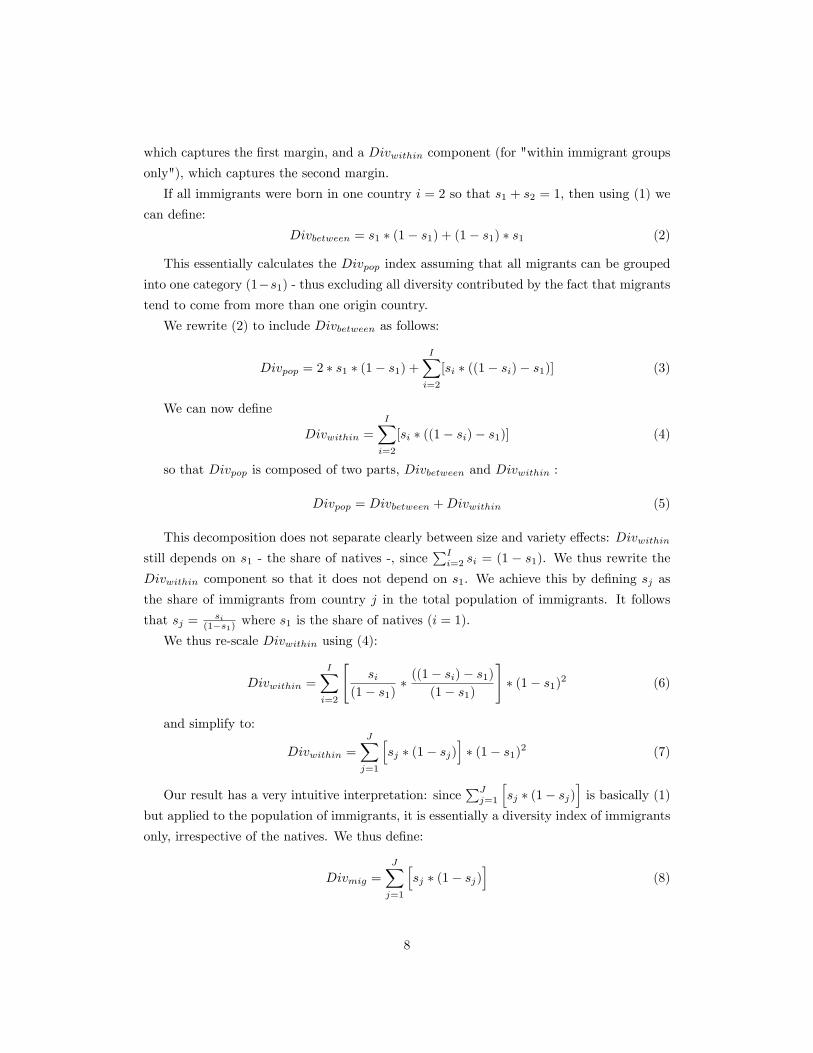
which captures the first margin, and a Divwithin component (for "within immigrant groups

only"), which captures the second margin.

If all immigrants were born in one country i = 2 so that s1 + s2 = 1, then using (1) we

can define:

Divbetween = s1 ∗ (1− s1) + (1− s1) ∗ s1 (2)

This essentially calculates the Divpop index assuming that all migrants can be grouped

into one category (1−s1) - thus excluding all diversity contributed by the fact that migrantstend to come from more than one origin country.

We rewrite (2) to include Divbetween as follows:

Divpop = 2 ∗ s1 ∗ (1− s1) +I∑i=2

[si ∗ ((1− si)− s1)] (3)

We can now define

Divwithin =I∑i=2

[si ∗ ((1− si)− s1)] (4)

so that Divpop is composed of two parts, Divbetween and Divwithin :

Divpop = Divbetween +Divwithin (5)

This decomposition does not separate clearly between size and variety effects: Divwithinstill depends on s1 - the share of natives -, since

∑Ii=2 si = (1 − s1). We thus rewrite the

Divwithin component so that it does not depend on s1. We achieve this by defining sj as

the share of immigrants from country j in the total population of immigrants. It follows

that sj = si(1−s1) where s1 is the share of natives (i = 1).

We thus re-scale Divwithin using (4):

Divwithin =I∑i=2

[si

(1− s1)∗ ((1− si)− s1)

(1− s1)

]∗ (1− s1)2 (6)

and simplify to:

Divwithin =J∑j=1

[sj ∗ (1− sj)

]∗ (1− s1)2 (7)

Our result has a very intuitive interpretation: since∑Jj=1

[sj ∗ (1− sj)

]is basically (1)

but applied to the population of immigrants, it is essentially a diversity index of immigrants

only, irrespective of the natives. We thus define:

Divmig =J∑j=1

[sj ∗ (1− sj)

](8)

8

And rewrite (5)

Divpop = Divbetween + (1− s1)2 ∗Divmig (9)

where (1− s1)2 has an intuitive interpretation as scale parameter for Divmig.We can then rewrite (9) in terms of smig, the share of immigrants (defined as foreign-

born) and define smig = (1− s1):

Divpop = 2 ∗ smig ∗ (1− smig) + (smig)2 ∗Divmig (10)

We have thus an expression of Divpop purely as a function of the size and diversity of

immigration.

4 Empirical analysis

4.1 Birthplace diversity data

Our computation of birthplace diversity indices relies on the Artuc, Docquier, Ozden and

Parsons (henceforth ADOP, 2015) data set which provides a comprehensive 195x195 ma-

trix of bilateral migration stocks disaggregated by skill category (with or without college

education) and gender for the years 1990 and 2000. Immigrants are defined as foreign-born

individuals aged 25+ at census or survey date. The dataset is based on a comprehensive

data collection effort in the host countries. For few destinations (and even fewer in our

sample), offi cial census information is not available. ADOP (2015) thus rely on a gravity

model-based estimation of these cells.7 In our sample, only 10% of skilled immigrants are

estimated based on this methodology.8

Three caveats are in order. First, illegal immigration is not accounted for in most

censuses, although in some cases (like in the US census) it is estimated. However, this

limitation is mitigated by the fact that we use data on immigration stocks, not flows: most

illegal migrants eventually become legalized or return to their country of origin. Second,

immigrants who came as children are subsequently treated fully as immigrant workers (when

aged 25+). However, these children then grow up, socialize and go to school in the host

country, which puts a limit on the extent of variety in skills that they can contribute when

they integrate the labor force. We address this issue in a robustness check. Third, a

migrant is considered skilled independently of the location of college education, meaning

that skilled migrants may be heterogeneous in terms of human capital quality. We partly

7See ADOP (2015) for more details.8We conduct a robustness check restricting our OLS and IV models to non-estimated observations only.

The results (available upon request) remain virtually unchanged.

9

address this issue by controlling for what we call "origin-effects" and review implications for

our identification in Section 5.

4.2 Descriptive statistics and correlations

Table 1a shows the weak bilateral correlations between ethnic, genetic and birthplace diver-

sity measures. The correlation between ethnic fractionalization and Divmig (all) is negative

at -.11 and close to zero for Divmig (skilled).9 Table 1b shows summary statistics, Table 1c

presents our data sources.

There is ample variation in country level birthplace diversity: Canada, Italy, Israel,

Germany, Australia and the UK have high birthplace diversity of immigrants (Divmig). The

United States rank only 18th in a list of countries with the highest immigration diversity

(at .92) due to relatively low diversity for unskilled immigration (0.84). Similarly low ranks

can be observed for Germany (rank 27, at .90) and Australia (rank 28, at .90). In terms

of Divmig (skilled), however, the USA is very near the top (at .97). Countries with lowest

overall immigration diversity are Pakistan, Bangladesh, Nepal, Syria and Iran (all lower

than .5). Neighboring country effects seem to play a role: Ireland’s Divmig (.54 overall, .44

for the unskilled and .67 for the skilled) is still quite low due to dominant immigration from

the UK. Switzerland, Austria or Australia follow similar patterns. Generally, such effects

are more prevalent for Divmig (unskilled). As a result, Divmig (skilled) tends to be higher

than Divmig (unskilled). This is consistent with migrants’ self-selection being driven by

net-of-migration-costs wage differentials, where low migration costs (due to short distances

and high networks) mostly affect low-skill migration.10

Table 2 shows some multivariate correlations between ethnic, linguistic and genetic di-

versity (ancestry-corrected), birthplace diversity and income per capita. Unlike all other

dimensions of diversity, Divpop is positively correlated with income per capita (at PPP),

while ethnic and linguistic fractionalization are negatively correlated. Genetic diversity’s

effect on income follows an inverted u-shape (Ashraf and Galor, 2013a). When we include

population birthplace diversity (Divpop), coeffi cients on the other diversity variables change

insignificantly. The inclusion of birthplace diversity, however, adds considerably to the pre-

dictive power of the model. We interpret this as indication thatDivpop is correlated with and

jointly determined by many other factors, such as geography or the quality of institutions.

Interestingly, this seems to be more an issue for the diversity of the unskilled population,

and generally this is driven to a lower extent by the variety than by the size of immigration.

9This also holds in first differences: the correlation between changes in size and diversity of skilled

immigration 1990-2000 is low and even negative at -.14.10See McKenzie and Rapoport (2010) and Bertoli (2010) for micro evidence on the role of migrant networks

in determining self-selection patterns, and Beine, Docquier and Ozden (2011) for macro evidence.

10

This point is further illustrated in models (6)-(8) where we use our decomposition analysis

and separate Divpop into Divbetween and Divwithin. The productive effects of Divpop clearly

vary by skill level: Divpop (unskilled) is mostly driven by Divbetween, but the association of

Divpop (skilled) with income per capita runs mostly through Divwithin. Still, Divbetween and

Divwithin are not independent from each other, as both depend on smig (see equations 2

and 4 above). We thus proceed with a model that includes a large range of co-determinants

of birthplace diversity and income. We also clearly separate the size (smig) and the variety

(Divmig) dimensions of birthplace diversity.

4.3 Model specification

To empirically investigate the relationship between birthplace diversity and economic de-

velopment, we specify the following model where our dependent variable y is a country’s

income per capita (GDP) at real PPP from the Penn World Tables 8.0 (Feenstra et al.,

2013):11

ln ykt = α+ β1 ∗Divmig kst + β2 ∗ smig kst+β3 ∗∆k + β4 ∗ Φk + β5 ∗Xk

+β6 ∗Ψkt + β7 ∗ Ωkt + β8 ∗ Γkt + ηt + e

where ∆k is a vector of fractionalization/diversity measures, Φk is a vector of climate

and geography characteristics, Xk is a vector of disease environment indices, Ψkt is a vector

of controls for institutional development, Ωkt is a vector of trade and origin effects, Γkt is a

vector containing the country’s population size and schooling level, and ηt is a period fixed

effect. We use indices s for skill groups (s=overall, skilled, unskilled), t for time periods

(1990, 2000) and k for countries.

The results from our decomposition analysis as well as our initial correlation analyses

point to the need to separate Divbetween and Divwithin further into their components, the

share of immigrants, smig, and the diversity of immigrants, Divmig. Thus we include the

share and the diversity of immigrants evaluated at the means of the respective variables. To

facilitate the interpretation we standardize both variables with a mean of zero and standard

deviation of one. In the appendix we also test for interaction effects between size and variety.

Our baseline specification starts with a parsimonious model based upon Table 2 where we

control for fractionalization/diversity indices (∆k) only. We specifically include both ethnic

and linguistic fractionalization (from Alesina et al., 2003) and genetic diversity (ancestry-

adjusted) from Ashraf and Galor (2013a) since all three indices capture a potentially different

productive margin of diversity.12

11See the online appendix for details on the definitions and sources for all variables.12Following Ashraf and Galor (2013a) we also include a squared term for genetic diversity.

11

We add more controls, going for increasingly stringent specifications incorporating first

exogenous geographic/climatic controls only (our vector Φk); we follow the literature on the

geographical determinants of income13 in including a landlockedness dummy (from CEPII,

2010), absolute latitude and share of population living within 100km of an ice-free coast

(both from Gallup et al., 1998), average temperature and precipitation (World Bank, 2013),

as well as a set of regional fixed effects for Latin America, Asia, Middle East and Northern

Africa (MENA), and Sub-Saharan Africa. We then add the semi-exogenous geographical

controls for the disease environment (Xk), which include malaria, yellow fever and tubercu-

losis incidence (all from World Bank, 2013).

We further extend the model to account for endogenous variables that co-determine

income and migration patterns. For institutional quality (Ψkt), we use the revised com-

bined Polity-2 score from the Polity IV database (Marshall and Jaggers, 2012). This index

measures the degree of political competition and participation, the degree of openness of

political executives’ recruitment and the extent of executives’ constraints (Glaeser et al.,

2004). We also add dummies for British, French and Spanish ex-colonies as proxies for the

origins of the legal system (CEPII, 2010).

Then comes our "trade and origin effects" vector, (Ωkt), which contains controls for the

volume and structure of trade (namely real trade openness from PWT 8.0),14 measures of

trade diversity in imports and exports (based on Feenstra et al., 2005),15 and also includes a

weighted average of the GDP per capita (in PPP) of immigrants’origin countries. The trade

diversity indices are the goods market equivalents ofDivmig, since import diversity is a proxy

for variety in (imported) intermediary goods. Controlling for trade is also necessary since

trade is determined by similar factors as migration (Ortega and Peri, 2014). Surprisingly

however, Divmig and variables of trade openness/diversity are not much correlated (+.08

for trade openness, +0.12 for trade diversity). Last, the "origin-effects" variable captures

the income at origin of the average representative immigrant and - while not a proxy for

the selection of immigrants from each country of origin - correlates with immigrant groups’

ability to cover migration costs. Richer destination countries that draw on (relatively) richer

source countries should be able to attract a wider range of immigrant groups and have higher

immigrant diversity. Controlling for such origin-effects allows us to account for differences

in migrant backgrounds (and skills) and focus on the pure (birthplace) diversity effect of

immigration. Finally, we include a vector (Γkt) containing education as captured by years

13See, e.g., Hall and Jones (1999), Gallup et al. (1998), Rodriguez and Rodrik (2001), Sachs (2003),

Rodrik et al. (2004).14We use the standard measure of trade volume: real trade openness (exports+imports) in percentage of

GDP in real PPP prices. This indicator correlates most robustly with GDP growth (Yanikkaya, 2003).15This definition follows the literature on trade concentration. See, e.g., Kali et al. (2007) for the effect

of trade concentration on income or Frankel et al. (1995) on transportation costs.

12

of education (Barro and Lee, 2013) and population size (U.N. Population Division, 2013).

We end up with a highly structured model and a short panel of 120 countries with data

for 1990 and 2000. We made a significant effort to broaden our sample. The 120 countries

reflect the intersection of the ADOP (2015) data, which is available for 190 countries and

territories (195 origins, but no immigration data for five destinations), the PWT 8.0 data,

which does not contain GDP data for 26 of those, the education data (Barro and Lee,

2013) which is not available for 25 remaining countries and other data sources (primarily

Alesina et al. 2003 and Ashraf and Galor, 2013a) where missing data drops another 19

countries.16 Our full sample does not differ systematically from a broader sample at the

intersection of PWT 8.0 and ADOP (2015). Differences in sample means are small (not

statistically significant) for most variables, with two exceptions: the sample mean for smigof skilled people is actually lower in our full sample than in the broader sample, and the

sample mean for Divmig is slightly higher (see the appendix for details). This reflects the

fact that we drop mainly small island states and territories that have very few skilled natives

and correspondingly higher smig (skilled) as well as experience immigration from few large

neighboring countries (leading to a lower Divmig). Still, after these slight reductions of the

sample size, our full sample still covers 90% of all global migrants and 93.7% of all skilled

migrants.

4.4 OLS results

We estimate our model using an OLS estimator with standard errors clustered at the country

level to account for serial correlation of standard errors. Our results are presented in Tables

3-5. Table 3 shows the full model estimated in a sample of 120 countries. In Table 4, we split

our sample into two sub-samples of rich vs. poor countries and establish our main results.

In Table 5 we analyze the stability of our main coeffi cients of interest by introducing groups

of controls sequentially as described above.

Table 3 shows the full model results for our two margins of birthplace diversity, smig and

Divmig, and does so separately for each skill level (overall, high- and low-skill). Both the

size of immigration and its diversity correlate positively with income at the 1% statistical

significance level. We report standardized coeffi cients for our key variables of interest to

facilitate interpretation. Coeffi cients for Divmig (skilled) are somewhat higher than those

for Divmig (unskilled), but this difference is not statistically significant. Once we control

for geographic variables (Michalopoulos 2012) ethnic and linguistic fractionalization con-

verge towards zero. Genetic diversity shows the expected inverted u-shaped pattern (Ashraf

and Galor, 2013a). Trade openness (Frankel and Romer, 1999), the quality of institutions

16Typical countries that drop out of this sample are small island states or territories.

13

(Acemoglu et al. 2001, Glaeser et al., 2004) and the level of education correlate positively

with economic development. These findings are consistent with the argument that both

the birthplace diversity of migrants as well as the share of immigrants relate positively to

economic development.

Table 4 shows sub-sample results for rich and poor countries (above or below median

GDP/capita in 1990). Given the theoretical arguments outlined in Section 2, we expect

the birthplace diversity (Divmig) of skilled workers to capture production function comple-

mentarities to a higher degree than other diversity indices. These complementarities should

also be larger in countries closer to the technology frontier. Hence, our estimates for Divmig(skilled) should be larger and more significant in a subset of rich economies relative toDivmig(unskilled) and relative to estimates in a poor country subsample. This is exactly what we

find. In the rich country subsample (column 2), our estimates for the standardized Divmig(skilled) are now considerably magnified vis-a-vis the full sample and remain significant at

the 1% level. When we conduct a horse-race of skilled and unskilled Divmig (column 4),

we find that our results for Divmig (skilled) continue to hold whereas the effect of Divmig(unskilled) are close to zero. In the poor country subsample (columns 5-8) we find no statis-

tically significant results for birthplace diversity. These results are consistent with the view

that the economic value of birthplace diversity for countries closer to the technology frontier,

particularly that arising from the diversity of skilled immigrants.17 Interestingly, neither

ethnic fractionalization nor linguistic or genetic diversity correlate robustly with income for

these countries.

Our identification strategy is potentially exposed to omitted variables bias, since within-

country variation in Divmig is very low and is thus an insuffi cient basis for identification.18

To address this concern at least partially, we specify in Table 5 a range of models that

sequentially introduce our controls. We analyze the stability of our main coeffi cients of

interest (on birthplace diversity of skilled immigrants) for rich countries (based on Table

4). Our estimates for Divmig (skilled) are stable across specifications. The coeffi cient

increases when going from model (1) to model (2), where we add a host of geography

controls (including, most importantly, our set of regional fixed-effects). All subsequent

model expansions do not substantially affect our coeffi cient estimates. In the last model

(column 6) we add population size and education controls, two variables that are positively

related to income and diversity. This slightly decreases the point-estimate for Divmig as this

likely takes out a small residual positive omitted variables bias. Interestingly, the relative

stability of our Divmig coeffi cient is not mirrored in our results for smig (skilled). Here, the

17The difference in Divmig (skilled) between the rich and poor country subsample is significant at the 1%

level (unlike the diversity of unskilled migrants).18Still, we obtain qualitatively similar results in our rich country subsample when using country fixed

effects (see Appendix).

14

coeffi cient varies substantially across specifications. This suggests that - as we discuss below

- Divmig is less likely to be affected by endogeneity issues than smig.

To add more structure to the analysis, we follow Oster (2013) who proposes a simple

heuristic to calculate bounding values for unbiased coeffi cients.19 The results following this

procedure indicate that any remaining omitted variables bias in our rich country subsample

model is negative but relatively small, as Oster’s bounding values for unbiased coeffi cients

are higher but in close proximity to our OLS estimates (see Table 5, column 6).

4.5 Robustness

4.5.1 Patenting activity

We extend our model to patent data in order to shed more light on the productivity effects

of Divmig (see Table 6). We define average patent intensity as the average number of

patent applications per capita filed by country nationals and registered by national patent

offi ces. We obtain this data from the World Intellectual Property Organization (2010) for

the period 1995-2005 and construct this measure for 117 countries.20 We apply our baseline

model using all covariates on a year 2000 cross section. We find that the diversity of

immigrants - in particular that of skilled immigrants - is robustly positively related to

scientific innovation as measured by patenting activity. This holds both for measures of

patent applications and patents granted per capita. These results hold also in our subsample

of richer countries. We do not find similar effects for the diversity of unskilled workers. We

take this as indication that the productivity-enhancing effect of variety in backgrounds and

problem solving heuristics embedded in Divmig partly works through innovation.

4.5.2 Total factor productivity

GDP/capita at PPP is our main dependent variable and we interpret the results for birth-

place diversity as indicative of skill complementarities. Our interpretation implies that the

effect of birthplace diversity should affect GDP/capita through total factor productivity

(TFP). To test this proposition, we replace our measure of GDP by a measure of TFP per

capita from the Penn World Tables 8.0 (Feenstra et al., 2013). Table 7 shows the results.

In both the full sample as well as the rich country subsample, birthplace diversity of skilled

immigrants remains positive and highly robust (at 1%). This suggests that, consistently

with an interpretation of the results in terms of skill complementarities, birthplace diversity

19This test relies on the assumption that selection on observables from a basic model towards a full model

is proportional to selection on unobservables.20The sample thus includes all countries with patenting activity as covered by WIPO (2010). Hence, our

estimates are best interpreted as effect on the intensive margin of patenting.

15

affects income via total factor productivity.

4.5.3 Second-generation effects

Immigration flows are highly time persistent due to network effects. This means that our

first-generation measure Divmig could capture also second/third-generation effects of im-

migration, biasing our results. We thus construct a measure of Divmig in 1960 based on

data from Ozden et al. (2011) to obtain a lagged birthplace diversity index and add this

new index and a lagged share of immigration to our model (see Table 8).21 As can be seen

in Column 2, the birthplace diversity of immigration in 1960 is positive but not significant

while the size of immigration in 1960 is positive and significant when these lagged variables

are entered independently of their contemporaneous values. Importantly, our main results

for first-generation birthplace diversity and for immigration size remain positive and highly

significant when past and present immigration size and diversity are entered jointly, with

point-estimates which are barely affected. In particular, the magnitude of Divmig remains

virtually unchanged, despite the high positive correlation between Divmig today and in the

past (+0.66). This suggests that skilled diversity’s productive effects in high income coun-

tries - our main finding - operate primarily through first-generation effects. This finding

is fully consistent with the theoretical arguments outlined in Section 2. The lack of sig-

nificance of past diversity, on the other hand, is consistent with an interpretation in terms

of compensating effects of birthplace and ethnic diversity (second-generation immigration

being a mix of the two).

4.5.4 Children immigrants

Our measure of Divmig counts all foreign-born workers as immigrants irrespective of the

duration of their stay in their host country. Immigrants arriving in the destination country

as children are - in terms of education and exposure to the destination country - probably

closer to being native than foreign. We thus compute Divmig and smig (skilled) at different

age-of-entry thresholds, using data for a subset of 29 OECD destination countries from Beine,

Docquier and Rapoport (2007). We find that our estimates for birthplace diversity are robust

to the exclusion of such special immigrant groups. We find somewhat lower estimates for

these corrected birthplace diversity measures (the difference is not statistically significant),

a fact that may be driven by attenuation bias due to counterfactual re-classification of young

immigrants as natives.

21Note that Ozden et al. (2011) do not provide a skill decomposition of immigration in 1960, we hence

rely on diversity of immigrants of all skill groups.

16

4.5.5 Outliers and alternative fixed effects

In a last step, we test the robustness of our results to the introduction of alternative re-

gional fixed effects as well as to excluding outliers (see Table 10). More specifically, Aus-

tralia, Canada and New Zealand have points-based immigration systems that select skilled

immigrants according to labor market needs. The United States attracts a huge part of

all skilled migrants in the world thanks to its large (pre and post tax) premium for skilled

labor (Grogger and Hanson, 2011). Controlling for these countries (in Column 3) or simply

dropping them from the sample (in Column 4) does not affect our results. Likewise, this

also holds for OPEC countries. In addition, we test robustness to alternative sets of fixed

effects to establish robustness for our within-geographic region estimator.22 Our results are

fully robust to these modifications.

5 Identification

5.1 Unobserved heterogeneity

Our measures of Divpop and Divmig rely on the assumption that we cover representative

individuals for the respective emigrant populations at different origins, and that immigrants

across destinations are homogenous. Since we lack detailed information on these migrants

(apart from education, gender and age-of-entry), we cannot exclude the possibility that

migrants are positively self-selected from the home-country pool of skilled workers and also

positively sort themselves to high-income destinations.23

In a first step, we use the ADOP (2015) dataset to calculate the relative degree of

selection per country of origin and destination based on observable skills. We calculate the

distribution of educational attainment (% of skilled) for the natives of any origin country

i from Barro and Lee (2013) and ADOP (2015) before emigration and immigration take

place. We then calculate the share of skilled emigrants from origin i to any destination k

and define:

skill selectionk =J∑j=1

skilled migrantsjktotal migrantsjk

skilled native bornjtotal native bornj

∗ smig jk

(11)

where k is an index for destination country, j for origin country, and smig jk is the share

of immigrants from origin j over all immigrants to destination k in year t. This index

is a weighted average of immigrants’ skills relative to the skill distribution of their home

countries’native population. A value of 1 indicates that migrants from j to k are identical

in terms of observed skills to non-migrants, a value above 1 signals positive selection. The

22 In particular, we test for robustness to continental fixed effects as employed by Ashraf and Galor (2013a).23See Grogger and Hanson (2011) for a deeper discussion on such sorting across destinations.

17

index may reflect skill-selective policies in destination countries as much as it reflects the

relative attractiveness of a destination country to skilled workers. Both aspects should be

correlated with selection on unobservables, since both are proxies for the relative return to

high skill, effort and risk taking attitudes. Clearly, our index of skill selection is at best an

imperfect and noisy measure of the true degree of positive selection. Still, skill selection is

positively correlated with income/capita at destination (+.34), even more than our origin

effects variable (+0.17) that accounts for destination countries’over-sampling of immigrants

from richer origins.

We proceed by adding the index of skill selection to our full model (Table 11, columns

2 and 3). The index and our origin effects variable both possess independent explanatory

power in a parsimonious model (column 2). This serves as indicative evidence that the

inclusion of these indices indeed mitigates the issue of migrant selection to some degree.

Column 3 shows full model results, indicating that once we condition on the full set of

controls, both indices lose their predictive power, while the coeffi cient on our key variable of

interest Divmig remains robustly estimated and statistically significant at the 1% level. The

estimate is slightly lower than in our base model, indicating the removal of a small positive

bias in our estimate.

We test the robustness of our findings further by dropping countries with the highest

skill selection from our sample. These are Australia, Belgium, Canada, Singapore, United

Kingdom and the USA. Their relative attractiveness reveals a preference of highly skilled

(and, presumably, highly motivated) workers towards destinations with higher returns to

skill and effort. Table 11, column (4) shows that our estimation does not depend on these

countries.

In a second step, we employ an alternative indirect measure of selection. We use data

collected by Gallup market research reported in Espinova et al. (2011). These authors

report an index of net migration potential that is based on surveys of close to 348.000 adults

between 2007 and 2010 and available for 148 countries. The index is based on answers to

the question "Ideally, if you had the opportunity, would you like to move permanently to

another country, or would you prefer to continue living in this country?" and is defined as

the potential percentage increase in the destination country population. The index is thus

effectively an indicator of attractiveness as it gives the potential share of immigration if there

were no constraints on migration. Besides the "usual suspects", countries like Botswana

and Malaysia make the TOP 20 due to their relative regional attractiveness. In addition

to controlling for this index (Table 11, column 5), we regress it on actual immigration

(smig) and birthplace diversity (Divmig) and add the residuals from these regressions to our

full model (columns 6 and 7). These residuals can be interpreted as the degree to which

18

existing constraints to immigration both at origin and destination countries are binding.24

Constraints to emigration in the origin countries and constraints in destination countries

both serve to increase the extent of migrants’skill-selection. Throughout models (5) to (7),

we find our estimates for Divmig to remain robust at the 1% level, albeit at slightly lower

magnitudes. This suggests that our main OLS findings are robust to alternative indirect

measures of selection.

In a third step, we use data provided by the OECD (2009) that capture the quality of

education in a range of OECD and non-OECD countries based on standardized (PISA) test

scores.25 Figure A3 in the appendix shows the distribution of countries’mean overall PISA

score for high school students at age 15. We re-compute our Divmig indices and exclude

countries of origin with scores exceeding the OECD average (e.g. Finland, Hong Kong,

Singapore). Countries that draw most heavily on such origins are - on average - more likely

to attract above average talent and thus have a higher chance to benefit from "superstar"

effects. Table 11, model (8) shows that the exclusion of these immigrants does not change

our results.

Next, we use the full distribution of highly-skilled math- and science students (namely,

the share of pupils per country in the highest sextile bracket of math and science skills

worldwide - see appendix for more details). The quality of education around the world,

especially outside the OECD, is remarkably poor.26 Thus, very few countries have a deep

pool of highly skilled individuals. We formalize this insight by calculating the maximum

population in each country of origin that could theoretically be classified as "highly-skilled"

in terms of mathematical skills. In essence, we apply the share of pupils in the top sextile

of math skills today to the entire population born in a given country (before emigration

and immigration), make very conservative assumptions (e.g., that the gap between rich and

poor countries’ educational quality is stable over time) where we encounter missing data

and compare that theoretical maximum of highly (math-) skilled people in each country

with the stock of actual (subsequent) emigration. The appendix provides more details on

the calculation. Given the very low numbers of highly skilled students outside the OECD,

the emigrant stock of skilled workers of many countries in the world greatly exceeds even an

optimistic hypothetical stock of highly math-skilled workers in these countries.27 In other

24 In line with our priors, in a basic model as in Table 11, column (2), both indices hold independent

explanatory power and correlate highly positively with income (available upon request).25See www.oecd-ilibrary.org (PISA 2009 results at a glance).26See Filmer, Hasan and Pritchett (2006), for an illustrative review of test score results. They report,

among many other examples, that "the average science score among students in Peru [is] equivalent to that

of the lowest scoring 5 percent of US students".27See the appendix for a simulation. The figures show that the vast majority of countries — even under

the assumption that all high-ability math/science students had left —mostly sent non- highly math-skilled

people abroad.

19

words, it is very unlikely for a rich country (with the possible exception of the mentioned

top few destinations) to attract highly-skilled migrants without specializing on just a few

countries with deep talent pools. Thus, for any not highly sought-after destination, more

Divmig necessarily implies less —not more —skill selection.

We test the robustness of our estimates for Divmig by dropping all immigrants from ori-

gins with large pools of highly talented workers (i.e., with a ratio of math/science-talented

workers / skilled emigrants > 1) from our calculation of Divmig. We thus obtain a coun-

terfactual index of birthplace diversity that disregards potential "high quality" immigrant

groups (see Table 11, columns 9 and 10). Our estimates are very comparable in terms of

magnitude and significance to our baseline Divmig index. This suggests that the inclusion of

immigrant groups with the highest likelihood for "superstar" backgrounds in our diversity

index does not observably drive our results.

Overall, our baseline specification remains fairly robust to empirical and conceptual

challenges to identification arising from the issue of selection on unobservables. Our main

result for the diversity of skilled immigrants survives the introduction of an index of skill-

selection based on observable skills as well as various adjustments to exclude immigrants

from source countries that either possess deep "talent pools" (i.e., where the national average

score on the standardized PISA test exceeds the cross-country OECD average) or that are

not "highly-skilled constrained" (i.e., where the ratio of an imputed number of highly-

talented workers in math/sciences skills to the overall number of skilled emigrants is larger

than unity). It is therefore plausible that only a minor fraction of our overall effect can be

explained by such selection. To the contrary, given that the pools of extra-ordinary high

achievers (with high cognitive abilities in science and math fields) are relatively shallow, it

seems that drawing skilled immigrants from a wide range of countries (and thus attaining

a high Divmig) is likely even correlated with a lower degree of selection of the best and the

brightest.

5.2 Reverse causality

Richer countries could attract a larger flow of immigrants (resulting in a higher smig) coming

from a wider range of origin countries (Divmig) simply because they are richer. An initial

descriptive analysis shows that the pure bilateral correlation with income, particularly for

skilled immigrants, is higher for smig (+0.32) than for Divmig (+0.23). This is even more

prevalent in first differences: changes in smig between 1990 and 2000 are clearly positively

associated with changes in income per capita (at 1% level), but changes in diversity are not

(the effect is close to zero and is not estimated precisely). Indirect effects from growth via

smig to Divmig appear also unlikely, since the correlation between a change in smig and a

20

change in Divmig is clearly negative (-0.36, significant at 5%).

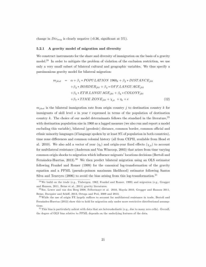
5.2.1 A gravity model of migration and diversity

We construct instruments for the share and diversity of immigration on the basis of a gravity

model.28 In order to mitigate the problem of violation of the exclusion restriction, we use

only a very small subset of bilateral cultural and geographic variables. We thus specify a

parsimonious gravity model for bilateral migration:

mjkst = α+ β1 ∗ POPULATION 1960k + β2 ∗DISTANCEjkt+β3 ∗BORDERjkt + β4 ∗OFF.LANGUAGEjkt+β5 ∗ ETH.LANGUAGEjkt + β6 ∗ COLONYjkt+β7 ∗ TIME ZONEjkt + χjt + ηt + e (12)

mjkst is the bilateral immigration rate from origin country j to destination country k for

immigrants of skill level s in year t expressed in terms of the population of destination

country k. The choice of our model determinants follows the standard in the literature,29

with destination population size in 1960 as a lagged measure (we also run and report a model

excluding this variable), bilateral (geodesic) distance, common border, common offi cial and

ethnic minority languages (if language spoken by at least 9% of population in both countries),

time zone differences and common colonial history (all from CEPII, available from Head et

al. 2010). We also add a vector of year (ηt) and origin-year fixed effects (χjt) to account

for multilateral resistance (Anderson and Van Wincoop, 2003) that arises from time varying

common origin shocks to migration which influence migrants’locations decisions (Bertoli and

Fernández-Huertas, 2013).30 We then predict bilateral migration using an OLS estimator

following Frankel and Romer (1999) for the canonical log-transformation of the gravity

equation and a PPML (pseudo-poisson maximum likelihood) estimator following Santos

Silva and Tenreyro (2006) to avoid the bias arising from this log-transformation.31

28We build on the trade (e.g., Tinbergen, 1962, Frankel and Romer, 1999) and migration (e.g., Grogger

and Hanson, 2011, Beine et al., 2011) gravity literatures.29See, Lewer and van den Berg 2008, Felbermayr et al. 2010, Mayda 2010, Grogger and Hanson 2011,

Beine, Docquier and Schiff, 2013, Ortega and Peri, 2009 and 2013.30While the use of origin FE largely suffi ces to account for multilateral resistance in trade, Bertoli and

Fernández-Huertas (2013) show this to hold for migration only under more restrictive distributional assump-

tions.31This bias is particularly salient with data that are heteroskedastic (e.g., due to many zero cells). Overall,

the degree of OLS bias relative to PPML depends on the underlying features of the data.

21

5.2.2 Instrumentation and identification

Table 12a/b shows results for our gravity models. Generally, the models have suffi ciently

high explanatory power and seem appropriately specified (keeping in mind that they are

purposefully excluding potential determinants of destination countries’productivity). All

estimates on the migration determinants have the expected sign: destination country pop-

ulation in 1960 and bilateral distance enter negatively. Skilled migration is less constrained

by migratory distance, as theory would predict, and is less affected by border-effects. The

cultural proximity variables (common colonial relationship and common offi cial/ethnic mi-

nority languages) both enter positively, as expected.

We construct instruments for our two main variables of interest, skilled birthplace di-

versity and the share of skilled immigration, using the predicted bilateral migration shares

estimated from our PPML and OLS gravity models.32 We turn to comparing our instru-

ments for predicted diversity with actual Divmig (see Appendix Figure 2a). The correlation

between actual and predicted diversity is strong, suggesting a priori a strong instrument.

Furthermore, the instrument should be lower (higher) than actual diversity in richer (poorer)

countries. This is exactly what we find (see Appendix Figure 2b): a negative link between

GDP per capita at destination and the difference between actual and predicted Divmig. We

take this as indication that our gravity model yields an instrument which takes out at least

a part of any small but endogenous component in the diversity-income relationship.

Table 13 shows the first-stage results corresponding to our 2SLS models in Table 14.

Throughout the models (which start with one instrumented variable and extend to up to

three) we reject the null hypothesis of weak instruments both jointly (Kleibergen-Paap F-

test) and individually (Angrist-Pischke F-tests), as these statistics exceed the strictest or

(in model 3) second strictest Stock and Yogo (2005) critical values.33

There are two issues that could affect the validity of our identification. First, bilateral

omitted variables could be correlated with bilateral migration and also with destination

country GDP/capita; for example bilateral trade with a rapidly growing trade partner such

as China could affect the GDP (via TFP) of China’s neighboring trade partners. However,

Hsieh and Ossa (2011) find that China’s productivity growth has only very small positive

effects on neighbor countries’TFP. We also account for such effects econometrically by in-

cluding origin-year fixed effects. Our trade controls should adequately capture any residual

aggregate bias. Second, relative bilateral geography variables (such as distance, common

32To avoid violating the exclusion restriction via inclusion of a lagged measure of population size, we fully

rely on the more parsimonious model excluding this variable.33As is well known, the Stock and Yogo (2002) critical values are are appropriate under homoskedasticity

only. We report heteroskedasticity-robust clustered standard errors, which tend to be higher than those

obtained under the assumption of homoskedasticity.

22

language or border contiguity) may be correlated with absolute (unilateral) geography vari-

ables, a point first raised in the context of trade gravity models by Rodriguez and Rodrik

(2001). We account for that by including a very broad set of geography and disease variables

into our second-stage baseline model, including the geographical fixed effects as suggested

by these authors and conducting many robustness exercises on our geography variables.

The inclusion of geography variables in our main model also served to remove an apparent

negative omitted variables bias (see Table 5, column 2), suggesting that such an (unlikely)

remaining bias from geography variables if any, may increase (not decrease) our Divmigestimates.

5.2.3 2SLS results

Table 14 shows results from our full model using the 2SLS estimator. We compare our

baseline OLS specification in model (1) with alternative IV-specifications in models (2)-(4).

In (2), we first instrument solely our main variable of interest, Divmig, assuming that any

remaining endogeneity in our model (e.g., from smig) is negligible. Then in (3), we relax

this assumption and also instrument for smig. We confirm our prior OLS findings on skilled

Divmig at the 5% level in both models.34 The IV estimates appear very stable and somewhat

lower than our OLS estimates. This is closely in line with our expectation, namely that first,

the OLS model suffers (if at all) from a low negative omitted variables bias, and second, that

our OLS estimates may only mildly suffer from a positive bias due to selection or reverse

causality. Our IV estimates confirm these inferences to a large extent. The slightly lower

IV estimates suggest that the net effect of these two biases was positive and relatively small

(less than 10% of the estimate). In other words, the positive bias from selection/reverse

causality exceeded the negative bias from omitted variables and (if at all) measurement

error. When instrumenting for the share of immigration (model 3), our estimates for smigremain similar in magnitude but lose significance. This suggests - in line with our discussion

of omitted variables and selection - that establishing causality for smig is a bigger challenge

than for Divmig.

In model (4), we go one step further and also instrument for Divimports. We thus apply

our gravity model of migration determinants to trade, following Frankel and Romer (1999).

The strategy to obtain instruments from similar models is valid to the extent that the

model determinants for migration and trade are estimated differentially. Table 12b shows

that this is indeed the case. Our Divmig estimate remains remarkably robust, but the overall

model is weakly identified since the instruments for the diversity of trade and migration are

correlated. Needless to say, this approach is very demanding given the few degrees of freedom

34F-Tests on the excluded instruments and the joint instruments are well above the respective Stock and

Yogo (2002) critical values.

23

in our model and correlation structure between instruments. Remarkably, our estimate for

Divmig remains similar in magnitude but - as expected - loses some statistical significance

(it remains significant at the 10% level). This serves as indication that any endogeneity bias

in our OLS model is small and unlikely to drive our main results.

6 Does cultural distance matter?

Is birthplace diversity more valuable if immigrants are culturally similar or come from

richer origin countries? So far, our index does not capture such characteristics and assumes

all groups to be equidistant from each other. We now expand this well-established but

restrictive notion of diversity to shed more light on the transmission channels.

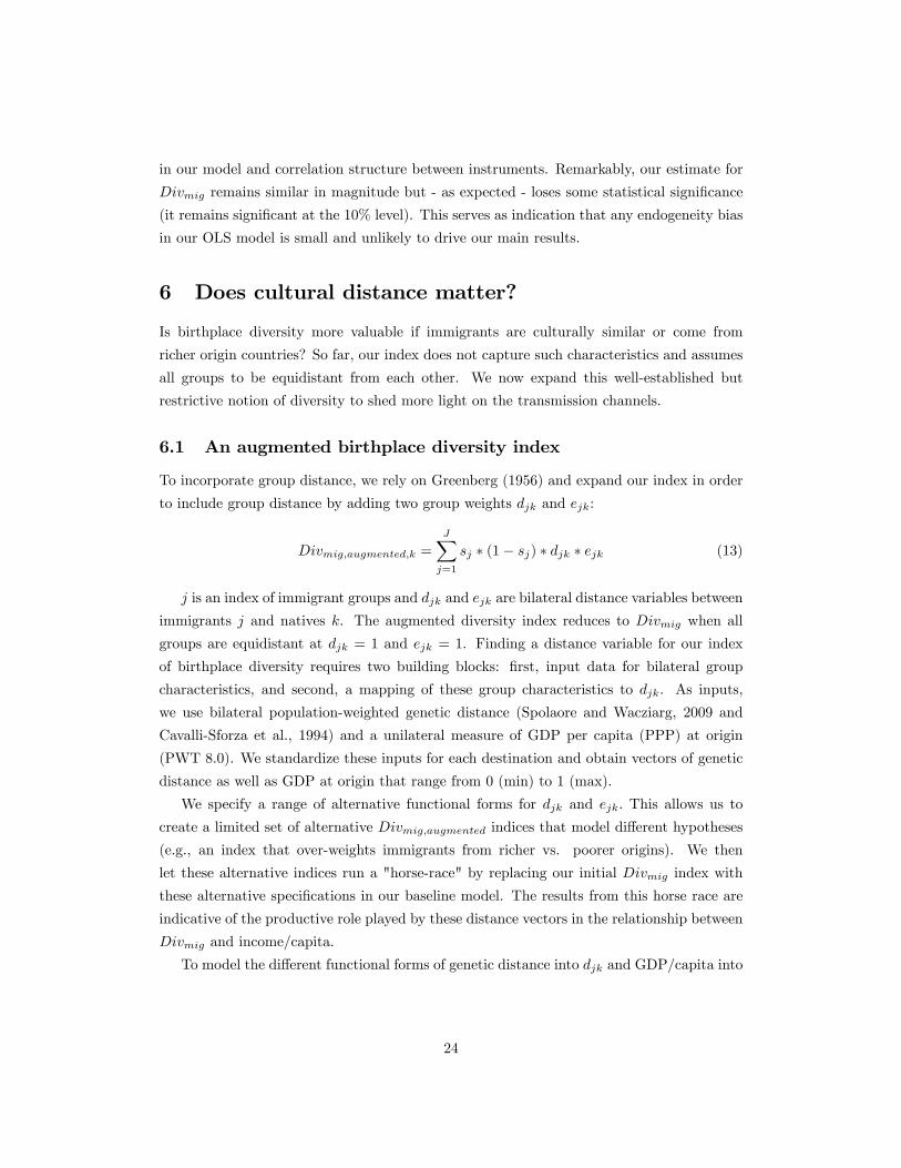
6.1 An augmented birthplace diversity index

To incorporate group distance, we rely on Greenberg (1956) and expand our index in order

to include group distance by adding two group weights djk and ejk:

Divmig,augmented,k =J∑j=1

sj ∗ (1− sj) ∗ djk ∗ ejk (13)

j is an index of immigrant groups and djk and ejk are bilateral distance variables between

immigrants j and natives k. The augmented diversity index reduces to Divmig when all

groups are equidistant at djk = 1 and ejk = 1. Finding a distance variable for our index

of birthplace diversity requires two building blocks: first, input data for bilateral group

characteristics, and second, a mapping of these group characteristics to djk. As inputs,

we use bilateral population-weighted genetic distance (Spolaore and Wacziarg, 2009 and

Cavalli-Sforza et al., 1994) and a unilateral measure of GDP per capita (PPP) at origin

(PWT 8.0). We standardize these inputs for each destination and obtain vectors of genetic

distance as well as GDP at origin that range from 0 (min) to 1 (max).

We specify a range of alternative functional forms for djk and ejk. This allows us to

create a limited set of alternative Divmig,augmented indices that model different hypotheses

(e.g., an index that over-weights immigrants from richer vs. poorer origins). We then

let these alternative indices run a "horse-race" by replacing our initial Divmig index with

these alternative specifications in our baseline model. The results from this horse race are

indicative of the productive role played by these distance vectors in the relationship between

Divmig and income/capita.

To model the different functional forms of genetic distance into djk and GDP/capita into

24

ejk we use a standard logistic function

djk =2(

1 + e−(θ∗xjk)) (14)

where θ is a parameter that ranges from -10 to +10 and xjk takes on standardized values

of genetic distance (for djk) and GDP/capita (for ejk). 35 The logistic function is convenient

for our purpose. It can be centered easily on djk = 1 for groups at average genetic proximity

(income) from the natives of a given per country and set to converge to two bounds 0 and 2.

In addition, by varying a single parameter θ, we can vary both the slope of the function and

the spread between genetically closer (poorer) and more distant (richer) groups. It assigns

djk and ejk values between 0 and 2 (centered on 1 for the theoretical case that all immigrant

groups are equidistant to natives). djk and ejk then act as group weights in the calculation of

Divmig,augmented. Larger absolute values of θ indicate a higher degree of relative over/under-

weighting. Augmented diversity indices based on θ > 0 overweight groups with higher

genetic distance (richer origins), those based on θ < 0 overweight closer groups (poorer

origins).The intuition is the following: if, say, genetically more distant (richer) groups were

more valuable in terms of explaining productivity differences, weighting these groups with

djk > 1 and correspondingly giving a lower weight of djk < 1 to genetically closer (poorer)

groups should result in an augmented birthplace diversity index that has higher explanatory

power in our model than its inverse index, one where we overweight closer (poorer) groups.

6.2 Results

Table 15 shows coeffi cients for Divmig (skilled) on a full range of alternative birthplace di-

versity indices at different combinations of θ1 and θ2. First, we interpret unilateral effects.

When holding GDP/capita constant (at θ2 = 0), giving more weight to culturally closer

immigrants (θ1 < 0) increases the predictive power of Divmig slightly - but excessively over-

weighting those diminishes the predictive power. In turn, overweighting culturally distant

groups (and thus relatively underweighting closer groups) clearly diminishes the effect of

Divmig on income. This nonlinear, concave pattern for genetic/cultural distance appears to

be very stable (even to a large extent when varying income at origin). It suggests a trade-

off between the productive costs and benefits of cultural distance. When holding genetic

distance constant at (θ2 = 0), the effect of Divmig increases somewhat linearly in income at

origin, but with a very small gradient than that of cultural proximity and also not monoton-

ically. This may suggest that the productive effects of Divmig (skilled) are driven to a larger

extent by culture than by income. We however cannot conclude this with certainty since

this interpretation is based on marginal, not average effects.35We use GDP/capita in origin countries only (not economic distance) to avoid including our dependent

variable in our regressor.

25

Second, we look at interaction effects. Moving from the center of Table 15 towards the

lower left corner (thus overweighting culturally closer immigrant groups and also overweight-

ing those from richer origins), the estimate on e.g., Divmig,augmented (θ1 = −2.5; θ2 = 10)

increases significantly (at 5% level) vs. the simple baseline index Divmig. This increase is

larger than any individual increase in either dimension (holding constant either θ1 or θ2 at

zero). This suggests that a combination of culturally closer immigrants and richer origins

(potentially a proxy for higher skills) can be particularly valuable.

7 Conclusion

We construct an index of population diversity based on people’s birthplaces. This new

index, which we decompose into a size (share of foreign born) and a variety (diversity of

immigrants) component, is available for 195 countries in 1990 and 2000 disaggregated by skill

level. Our birthplace diversity measures are conceptually and empirically orthogonal to the

various measures of diversity previously explored in the literature (such as ethnic, linguistic

or genetic diversity). We find that the diversity of (and arising from) immigration relates

positively to measures of economic prosperity. This holds especially for skilled immigrants

in richer countries. Increasing the diversity of skilled immigration by one percentage point

increases long run economic output by about two percent.36 These results are robust to our

attempts to account for potential reverse causality and unobserved heterogeneity among

skilled immigrants. They are also robust to using various sub-samples (and definitions of

countries), to accounting for immigrants’age of entry or to second-generation effects.

Lastly, we extend our index of birthplace diversity and account for cultural and economic

distance between immigrants and natives. The productive effects of birthplace diversity ap-

pear to be largest for immigrants originating from richer countries and from countries at

intermediate levels of cultural proximity. We interpret these findings as suggestive of the

trade-offs between communication and social costs of diversity and benefits in terms of pro-

duction function effects that arise from skill complementarities. Hence, birthplace diversity

is an important determinant of economic prosperity that is conceptually, empirically and

economically different from other (e.g., ethnic, linguistic or genetic) dimensions of intrapop-

ulation diversity.

36For a one standard deviation increase in birthplace diversity (skilled immigrants), this equals an increase

of about 25% in economic output.

26

8 References

Abramitzky, R., L. Boustan and K. Eriksson (2012), "Europe’s Tired, Poor, Huddled

Masses: Self-selection and Economic Outcomes in the Age of Mass Migration." American

Economic Review, 102(5): 1832-1856.

Abramitzky, R., L. Boustan and K. Eriksson (2013), "Have the Poor Always Been Less

Likely to Migrate? Evidence from Inheritance Practices during the Age of Mass Migration.”

Journal of Development Economics, 102: 2-14.

Acemoglu, D., S. Johnson and J. Robinson (2001), "The Colonial Origins of Comparative

Development: An Empirical Investigation." American Economic Review, 91(5): 1369-1401.

Ager, P. and M. Brückner (2013), "Cultural Diversity and Economic Growth: Evidence

from the US during the Age of Mass Migration." European Economic Review, 64: 76—97.

Alesina, A., R. Baqir and W. Easterly (1999), "Public Goods and Ethnic Divisions."

Quarterly Journal of Economics, 114(4): 1243-84.

Alesina, A., A. Devleeschauwer, W. Easterly, S. Kurlat and R. Wacziarg (2003), "Frac-

tionalization." Journal of Economic Growth, 8(2): 155-194.

Alesina, A. and E. La Ferrara (2000), "Participation in Heterogeneous Communities."

Quarterly Journal of Economics, 115(3): 847-904.

Alesina, A. and E. La Ferrara (2002), "Who Trusts Others?" Journal of Public Eco-

nomics, 85(2): 207-234.

Alesina, A. and E. La Ferrara (2005), "Ethnic Diversity and Economic Performance."

Journal of Economic Literature, 43(3): 762-800.

Alesina, A., S. Michalopoulos, and E. Papaioannou (2015), "Ethnic Inequality." Journal

of Political Economy, forthcoming.

Alesina, A., E. Spolaore, and R. Wacziarg (2000), "Economic Integration and Political

Disintegration." American Economic Review, 90(5): 1276-1296.

Alesina, A. and E. Spolaore (2005), "The Size of Nations." MIT Press, 2005.

Alesina, A. and E. Zhuravskaya (2011), "Segregation and the Quality of Government in

a Cross Section of Countries." American Economic Review, 101(5): 1872-1911.

Andersen, T. and C.-J. Dalgaard (2011), "Flows of People, Flows of Ideas, and the

Inequality of Nations." Journal of Economic Growth, 16(1): 1-32.

Anderson, J. and E. Van Wincoop (2003), "Gravity And Gravitas: A Solution To The

Border Puzzle." American Economic Review, 93(1): 170-192.

Artuc, E., F. Docquier, C. Özden and C. Parsons (2015), "A Global Assessment of

Human Capital Mobility: The Role of non-OECD Destinations." World Development, 65:

6-26.

Ashraf, Q. and O. Galor (2011), "Cultural Diversity, Geographical Isolation, and the

27

Origin of the Wealth of Nations." NBER Working Paper No. 17640.

Ashraf, Q. and O. Galor (2013a), "The Out of Africa Hypothesis, Human Genetic Diver-

sity and Comparative Economic Development." American Economic Review, 103(1): 1-46.

Ashraf, Q. and O. Galor (2013b), "Genetic Diversity and the Origins of Cultural Frag-

mentation." American Economic Review, 103(3): 528—533.

Bandiera, O., I. Rasul and M. Viarengo (2013): "The Making of Modern America: Migra-

tory Flows in the Age of Mass Migration." Journal of Development Economics, 102(May):

23-47.

Barro, R. and J. Lee (2013), "A New Data Set of Educational Attainment in the World,

1950-2010." Journal of Development Economics, Vol. 104: 184-198.

Beine, M., F. Docquier and H. Rapoport (2007), "Measuring International Skilled Mi-

gration: New Estimates Controlling For Age of Entry." World Bank Economic Review, 21:

249-254.

Beine, M., F. Docquier and C. Özden (2011), "Diasporas." Journal of Development

Economics, 95(1): 30-41.

Beine, M., F. Docquier and M. Schiff (2013), "Migration, Transfer of Norms and Home

Country Fertility." Canadian Journal of Economics, 46(4): 1406-1430.

Bellini E., G. Ottaviano, D. Pinelli and G. Prarolo (2013): "Cultural Diversity and

Economic Performance: Evidence from European Regions"; in R. Crescenzi and R. Percoco,

eds.: Geography, Institutions and Regional Economic Performance, Advances in Spatial

Science, Berlin and Heidelberg: Springer Verlag : 121-141.

Bertoli, S. (2010), "Networks, Sorting and Self-selection of Ecuadorian Migrants." An-

nales d’Economie et de Statistique, 97-98: 261-88.

Bertoli, S. and J. Fernández-Huertas Moraga (2013), "Multilateral Resistance to Migra-

tion." Journal of Development Economics, Vol. 102: 79-100.

Boeheim, R., G. Horvath and K. Mayr (2012), "Birthplace Diversity of the Workforce

and Productivity Spill-overs in Firms." WIFO Working Papers No. 438.

Brunow, S., M. Trax and J. Suedekum (2015), "Cultural Diversity and Plant-level Pro-

ductivity." Regional Science and Urban Economics, 53: 85-96.

Cavalli-Sforza, L. L., P. Menozzi and A. Piazza (1994), "The History and Geography of

Human Genes." Princeton University Press, Princeton.

Collier, P. (1999), "On the Economic Consequences of Civil War." Oxford Economic

Papers, 51: 168-183.

Collier, P. (2001), "Ethnic Diversity: An Economic Analysis of its Implications." Eco-

nomic Policy, 32: 129-166.

Desmet, K., I. Ortuño-Ortín and R. Wacziarg (2012), "The Political Economy of Eth-

nolinguistic Cleavages." Journal of Development Economics, 97(2): 322-338.

28

Docquier, F. and H. Rapoport (2012), "Globalization, Brain Drain and Development."

Journal of Economic Literature, 50(3): 681-730.

Easterly, W. and R. Levine (1997), "Africa’s Growth Tragedy: Policies and Ethnic

Divisions." Quarterly Journal of Economics, 112(4): 1203-1250.

Espinova, N., J. Ray and R. Srinivasan (2011), "The World’s Potential Migrants."

Gallup. Available from www.imi.ox.ac.uk/pdfs/the-worlds-potential-migrants. Last ac-

cessed: 23 March 2015.

Esteban, J. and E. Ray (1994), "On the Measurement of Polarization." Econometrica,

62(4): 819-51.

Esteban, J. and E. Ray (2011), "Linking Conflict to Inequality and Polarization." Amer-

ican Economic Review, 101 (4): 1345-74.

Esteban, J., L. Mayoral and E. Ray (2012), "Ethnicity and Conflict: An Empirical

Study." American Economic Review, 102(4): 1310-1342.

Fearon, J. (2003), "Ethnic and Cultural Diversity by Country." Journal of Economic

Growth, 8(2): 195-222.

Fearon, J. and D. Laitin (2003), "Ethnicity, Insurgency, and Civil War." American Po-

litical Science Review, 97(1): 75-90.

Feenstra, R., R. Lipsey, H. Deng, A. Ma and H. Mo (2005), "World Trade Flows: 1962-

2000." NBER Working Paper No. 11040.

Feenstra, R., R. Inklaar and M. Timmer (2013), "The Next Generation of The Penn

World Table." Available for download at www.ggdc.net/pwt.

Felbermayr, G., S. Hiller and D. Sala (2010), "Does Immigration Boost Per Capita

Income?" Economics Letters, 107(2): 177-179.

Fershtman, C., H. Hvide and Y. Weiss (2006), "Cultural Diversity, Status Concerns and

the Organization of Work." Research in Labor Economics, 24: 3-38.

Filmer, D. A. Hasan and L. Pritchett (2006), "A Millennium Learning Goal: Measuring

Real Progress in Education." Center for Global Development Working Paper 97.

Frankel, J. and D. Romer (1999), "Does Trade Cause Growth?" The American Economic

Review, 89(3): 379-399.

Frankel, J., E. Stein and S. J. Wei (1995), "Trading Blocs and the Americas: The Natural,

the Unnatural, and the Super-Natural." Journal of Development Economics, 47(1): 61-95.

Gallup, J., J. Sachs and A. Mellinger (1998), "Geography and Economic Development,"

in Pleskovic, B. and J.E. Stiglitz (eds.), Annual World Bank Conference on Development

Economics, The World Bank: Washington, DC.

Glaeser, E., R. La Porta and A. Shleifer (2004), "Do Institutions Cause Growth?" Journal

of Economic Growth, 9(4): 271-303.

Greenberg, J. (1956), "The Measurement of Linguistic Diversity." Language, 32: 109-115.

29

Grogger, J. and G. Hanson (2011), "Income Maximization and the Selection and Sorting

of International Migrants." Journal of Development Economics, 95: 42-57.

Hall, R. and C. Jones (1999), "Why do some Countries Produce so much more Output

per Worker than Others?" Quarterly Journal of Economics, 114(1): 83-116.

Hambrick, D., T. Seung Cho and M. J. Chen (1996), "The Influence of Top Manage-

ment Team Heterogeneity on Firms’Competitive Moves." Administrative Science Quarterly,

41(4): 659-684.

Hatton, T. and J. Williamson (1998), "The Age of Mass Migration: Causes and Economic

Impact." Oxford : Oxford University Press.

Head, K., T. Mayer and J. Ries (2010), "The Erosion of Colonial Trade Linkages after

Independence." Journal of International Economics, 81(1): 1—14.

Hjort, J. (2014), "Ethnic Divisions and Production in Firms." Quarterly Journal of

Economics, 129, 4: 1899-1946.

Hong, L. and S. Page (2001), "Problem Solving by Heterogeneous Agents." Journal of

Economic Theory, 97(1): 123-163.

Hoogendoorn, S. and M. van Praag (2012), "Ethnic Diversity and Team Performance:

A Field Experiment." IZA Working Paper No. 6731.

Hsieh, C. T. and R. Ossa (2011), "A Global View of Productivity Growth in China."

NBER Working Paper 16778, September 2011.

Kahane, L., N. Longley and R. Simmons (2013), "The effect of coworker heterogeneity

on firm-level output: assessing the impacts of cultural and language diversity in the National

Hockey League." Review of Economics and Statistics, 95, 1: 302-314.

Kali, R., F. Méndez and J. Reyes (2007), "Trade Structure and Economic Growth."

Journal of International Trade & Econ. Development, 16(2): 245-269.

Laitin, D. D. and S. Jeon (2013), "Exploring Opportunities in Cultural Diversity."

Mimeo, Stanford University.

Lazear, E. P. (1999a), "Globalisation and the Market for Teammates." Economic Jour-

nal, 109(454): 15-40.

Lazear, E. P. (1999b), "Culture and Language." Journal of Political Economy, 107(6):

95-126.

Marshall, M. and K. Jaggers (2012), "Polity IV Project: Political Regime Characteristics

and Transitions, 1800-2012." Center for International Development and Conflict Manage-

ment, University of Maryland.

Mayda, A. (2010), "International Migration: A Panel Data Analysis of the Determinants

of Bilateral Flows." Journal of Population Economics, 23(4): 1249-1274.

McKenzie, D. and H. Rapoport (2010), "Self-selection Patterns in Mexico-US Migration:

The Role of Migration Networks." Review of Economics and Statistics, 92(4): 811-821.

30

Michalopoulos, S. (2012), "The Origins of Ethnolinguistic Diversity." American Eco-

nomic Review, 102(4): 1508-1539.

Milliken, F. J. and L. L. Martins (1996), "Searching for Common Threads: Understand-

ing the Multiple Effects of Diversity in Organizational Groups." Academy of Management

Review, 21(2): 402-433.

Montalvo J. and M. Reynal-Querol (2005), "Ethnic Polarization, Potential Conflict and

Civil War." American Economic Review, 95(3): 796-816.

O’Reilly, C., D. Caldwell and W. Barnett (1989), "Work Group Demography, Social

Integration, and Turnover." Admin. Science Quarterly, 34(1): 21-37.

Oster, E. (2013), "Unobservable Selection and Coeffi cient Stability: Theory and Valida-

tion." NBER Working Paper 19054.

Ortega, F. and G. Peri (2009), "The Causes and Effects of International Migrations:

Evidence from OECD countries 1980-2005." NBER Working Paper 14833.

Ortega, F. and G. Peri (2014), "Openness and Income: the Roles of Trade and Migra-

tion." Journal of International Economics, 92, 2: 231-51.

Ottaviano, G. and G. Peri (2006), "The Economic Value of Cultural Diversity: Evidence

from U.S. Cities." Journal of Economic Geography, 6(1): 9-44.

Ozden, C., C. Parsons, M. Schiff and T. Walmsley (2011), "Where on Earth is Every-

body? The Evolution of Global Bilateral Migration 1960—2000." The World Bank Economic

Review, 25(1): 12-56.

Ozgen, C., P. Nijkamp and J. Poot (2013), "The Impact of Cultural Diversity on Firm:

Evidence from Dutch Micro Data." IZA Journal of Migration, 2, 18.

Parrotta, P., D. Pozzoli, and M. Pytlikova (2014), "Does Labor Diversity Affect Firm

Productivity?" European Economic Review, 66: 144—179.

Peri, G. (2012), "The Effect of Immigration on Productivity: Evidence from US States."

Review of Economics and Statistics, 94(1): 348-358.

Putnam, R. D. (1995), "Bowling Alone: America’s Declining Social Capital." Journal of

Democracy, 6(1): 65-78.

Reynal-Querol, M. (2002), "Ethnicity, Political Systems, and Civil Wars." Journal of

Conflict Resolution, 46(1): 29-54.

Rodriguez, F. and D. Rodrik (2001), "Trade Policy and Economic Growth: A Skeptic’s

Guide to the Cross-National Evidence." NBER Macroeconomics Annual, 15: 261-338.

Rodrik, D., A. Subramanian and F. Trebbi (2004), "Institutions Rule: The Primacy

of Institutions Over Geography and Integration in Economic Development." Journal of

Economic Growth, 9(2): 131-165.

Sachs, J. (2003), "Institutions don’t Rule: Direct Effects of Geography on Per Capita

Income." NBER Working Paper No 9490.

31

Santos Silva, J. and S. Tenreyro (2006), "The Log of Gravity." The Review of Economics

and Statistics, 88(4): 641-658.

Spolaore, E. and R. Wacziarg (2009), "The Diffusion of Development." Quarterly Journal

of Economics, 124(2): 469-529.

Stock, J. and M. Yogo (2005), "Testing for Weak Instruments in Linear IV Regression."

In Donald Andrews and James H. Stock, eds. Identification and Inference for Econometric

Models: Essays in Honor of Thomas Rothenberg, NY: Cambridge University Press.

Tinbergen, J. (1962), "An Analysis of World Trade Flows." in Shaping the World Econ-

omy, edited by Jan Tinbergen. New York: Twentieth Century Fund.

U.N. Population Division (2013): "World Population Prospects: The 2013 Revision."

availably at esa.un.org/wpp.

U.N. Statistics Division (2013): "Comtrade Database." available at comtrade.un.org.

World Intellectual Property Organization (2010), "World Intellectual Property Indica-

tors", http://www.wipo.int/ipstats/en/statistics/patents/.

Yanikkaya, H. (2003), "Trade Openness and Economic Growth: A Cross-Country Em-

pirical Investigation." Journal of Development Economics, 72(1): 57-89.

32

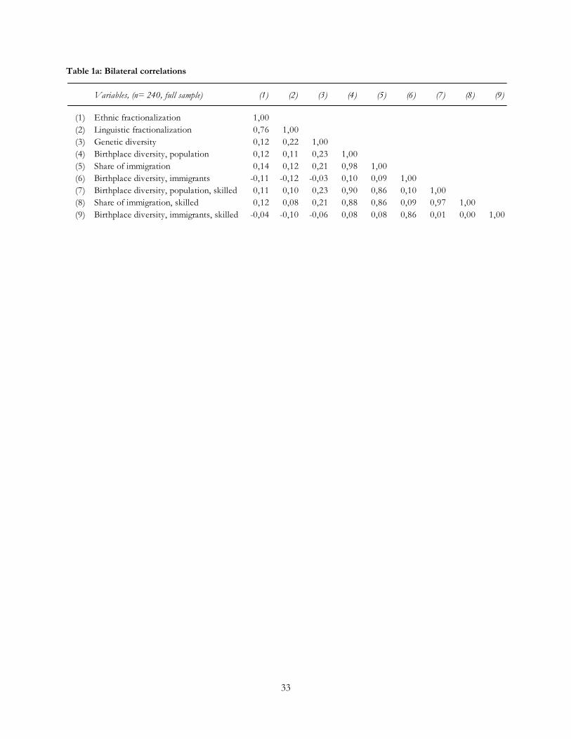
33

Table 1a: Bilateral correlations

Variables, (n= 240, full sample) (1) (2) (3) (4) (5) (6) (7) (8) (9)

(1) Ethnic fractionalization 1,00

(2) Linguistic fractionalization 0,76 1,00

(3) Genetic diversity 0,12 0,22 1,00

(4) Birthplace diversity, population 0,12 0,11 0,23 1,00

(5) Share of immigration 0,14 0,12 0,21 0,98 1,00

(6) Birthplace diversity, immigrants -0,11 -0,12 -0,03 0,10 0,09 1,00

(7) Birthplace diversity, population, skilled 0,11 0,10 0,23 0,90 0,86 0,10 1,00

(8) Share of immigration, skilled 0,12 0,08 0,21 0,88 0,86 0,09 0,97 1,00

(9) Birthplace diversity, immigrants, skilled -0,04 -0,10 -0,06 0,08 0,08 0,86 0,01 0,00 1,00

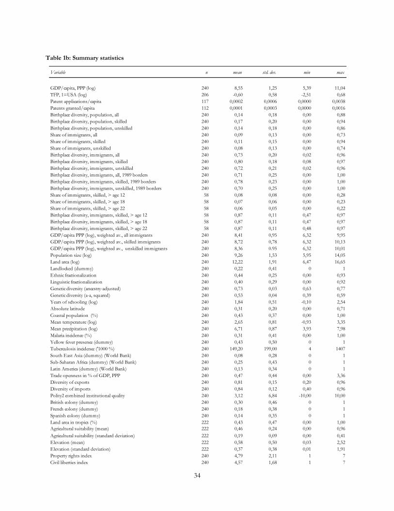
34

Table 1b: Summary statistics

Variable n mean std. dev. min max

GDP/capita, PPP (log) 240 8,55 1,25 5,39 11,04

TFP, 1=USA (log) 206 -0,60 0,58 -2,51 0,68

Patent applications/capita 117 0,0002 0,0006 0,0000 0,0038

Patents granted/capita 112 0,0001 0,0003 0,0000 0,0016

Birthplace diversity, population, all 240 0,14 0,18 0,00 0,88

Birthplace diversity, population, skilled 240 0,17 0,20 0,00 0,94

Birthplace diversity, population, unskilled 240 0,14 0,18 0,00 0,86

Share of immigrants, all 240 0,09 0,13 0,00 0,73

Share of immigrants, skilled 240 0,11 0,15 0,00 0,94

Share of immigrants, unskilled 240 0,08 0,13 0,00 0,74

Birthplace diversity, immigrants, all 240 0,73 0,20 0,02 0,96

Birthplace diversity, immigrants, skilled 240 0,80 0,18 0,08 0,97

Birthplace diversity, immigrants, unskilled 240 0,72 0,21 0,02 0,96

Birthplace diversity, immigrants, all, 1989 borders 240 0,71 0,25 0,00 1,00

Birthplace diversity, immigrants, skilled, 1989 borders 240 0,78 0,23 0,00 1,00

Birthplace diversity, immigrants, unskilled, 1989 borders 240 0,70 0,25 0,00 1,00

Share of immigrants, skilled, > age 12 58 0,08 0,08 0,00 0,28

Share of immigrants, skilled, > age 18 58 0,07 0,06 0,00 0,23

Share of immigrants, skilled, > age 22 58 0,06 0,05 0,00 0,22

Birthplace diversity, immigrants, skilled, > age 12 58 0,87 0,11 0,47 0,97

Birthplace diversity, immigrants, skilled, > age 18 58 0,87 0,11 0,47 0,97

Birthplace diversity, immigrants, skilled, > age 22 58 0,87 0,11 0,48 0,97

GDP/capita PPP (log), weighted av., all immigrants 240 8,41 0,95 6,32 9,95

GDP/capita PPP (log), weighted av., skilled immigrants 240 8,72 0,78 6,32 10,13

GDP/capita PPP (log), weighted av., unskilled immigrants 240 8,36 0.95 6,32 10,01

Population size (log) 240 9,26 1,53 5,95 14,05

Land area (log) 240 12,22 1,91 6,47 16,65

Landlocked (dummy) 240 0,22 0,41 0 1

Ethnic fractionalization 240 0,44 0,25 0,00 0,93

Linguistic fractionalization 240 0,40 0,29 0,00 0,92

Genetic diversity (ancestry-adjusted) 240 0,73 0,03 0,63 0,77

Genetic diversity (a-a, squared) 240 0,53 0,04 0,39 0,59

Years of schooling (log) 240 1,84 0,51 -0,10 2,54

Absolute latitude 240 0,31 0,20 0,00 0,71

Coastal population (%) 240 0,43 0,37 0,00 1,00

Mean temperature (log) 240 2,65 0,81 -0,93 3,35

Mean precipitation (log) 240 6,71 0,87 3,93 7,98

Malaria incidence (%) 240 0,31 0,41 0,00 1,00

Yellow fever presence (dummy) 240 0,43 0,50 0 1

Tuberculosis incidence ('1000 %) 240 149,20 199,00 4 1407

South East Asia (dummy) (World Bank) 240 0,08 0,28 0 1

Sub-Saharan Africa (dummy) (World Bank) 240 0,25 0,43 0 1

Latin America (dummy) (World Bank) 240 0,13 0,34 0 1

Trade openness in % of GDP, PPP 240 0,47 0,44 0,00 3,36

Diversity of exports 240 0,81 0,15 0,20 0,96

Diversity of imports 240 0,84 0,12 0,40 0,96

Polity2 combined institutional quality 240 3,12 6,84 -10,00 10,00

British colony (dummy) 240 0,30 0,46 0 1

French colony (dummy) 240 0,18 0,38 0 1

Spanish colony (dummy) 240 0,14 0,35 0 1

Land area in tropics (%) 222 0,43 0,47 0,00 1,00

Agricultural suitability (mean) 222 0,46 0,24 0,00 0,96

Agricultural suitability (standard deviation) 222 0,19 0,09 0,00 0,41

Elevation (mean) 222 0,58 0,50 0,03 2,52

Elevation (standard deviation) 222 0,37 0,38 0,01 1,91

Property rights index 240 4,79 2,11 1 7

Civil liberties index 240 4,57 1,68 1 7

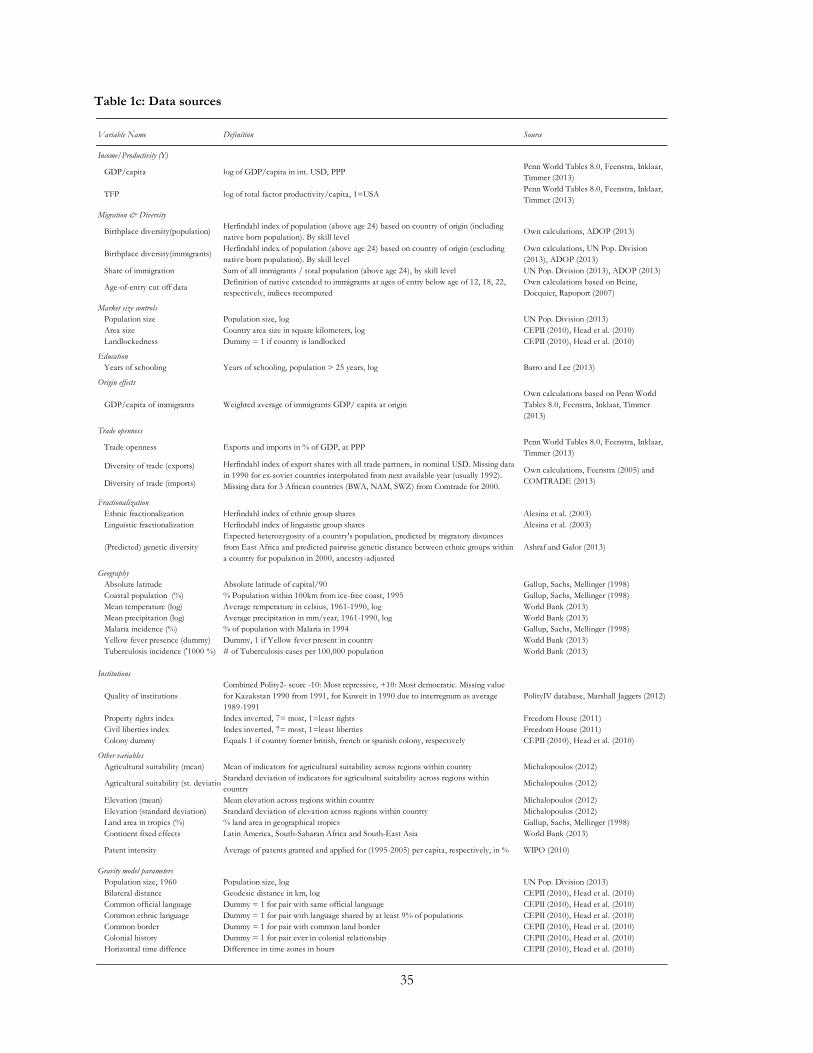
35

Table 1c: Data sources

Variable Name Definition Source

Income/Productivity (Y)

GDP/capita log of GDP/capita in int. USD, PPPPenn World Tables 8.0, Feenstra, Inklaar,

Timmer (2013)

TFP log of total factor productivity/capita, 1=USAPenn World Tables 8.0, Feenstra, Inklaar,

Timmer (2013)

Migration & Diversity

Birthplace diversity(population)Herfindahl index of population (above age 24) based on country of origin (including

native born population). By skill level Own calculations, ADOP (2013)

Birthplace diversity(immigrants)Herfindahl index of population (above age 24) based on country of origin (excluding

native born population). By skill level

Own calculations, UN Pop. Division

(2013), ADOP (2013)

Share of immigration Sum of all immigrants / total population (above age 24), by skill level UN Pop. Division (2013), ADOP (2013)

Age-of-entry cut off dataDefinition of native extended to immigrants at ages of entry below age of 12, 18, 22,

respectively, indices recomputed

Own calculations based on Beine,

Docquier, Rapoport (2007)

Market size controls

Population size Population size, log UN Pop. Division (2013)

Area size Country area size in square kilometers, log CEPII (2010), Head et al. (2010)

Landlockedness Dummy = 1 if country is landlocked CEPII (2010), Head et al. (2010)

Education

Years of schooling Years of schooling, population > 25 years, log Barro and Lee (2013)

Origin effects

GDP/capita of immigrants Weighted average of immigrants GDP/ capita at origin

Own calculations based on Penn World

Tables 8.0, Feenstra, Inklaar, Timmer

(2013)

Trade openness

Trade openness Exports and imports in % of GDP, at PPPPenn World Tables 8.0, Feenstra, Inklaar,

Timmer (2013)

Diversity of trade (exports)

Diversity of trade (imports)

Fractionalization

Ethnic fractionalization Herfindahl index of ethnic group shares Alesina et al. (2003)

Linguistic fractionalization Herfindahl index of linguistic group shares Alesina et al. (2003)

(Predicted) genetic diversity

Expected heterozygosity of a country's population, predicted by migratory distances

from East Africa and predicted pairwise genetic distance between ethnic groups within

a country for population in 2000, ancestry-adjusted

Ashraf and Galor (2013)

Geography

Absolute latitude Absolute latitude of capital/90 Gallup, Sachs, Mellinger (1998)

Coastal population (%) % Population within 100km from ice-free coast, 1995 Gallup, Sachs, Mellinger (1998)

Mean temperature (log) Average temperature in celsius, 1961-1990, log World Bank (2013)

Mean precipitation (log) Average precipitation in mm/year, 1961-1990, log World Bank (2013)

Malaria incidence (%) % of population with Malaria in 1994 Gallup, Sachs, Mellinger (1998)

Yellow fever presence (dummy) Dummy, 1 if Yellow fever present in country World Bank (2013)

Tuberculosis incidence ('1000 %) # of Tuberculosis cases per 100,000 population World Bank (2013)

Institutions

Quality of institutions

Combined Polity2- score -10: Most repressive, +10: Most democratic. Missing value

for Kazakstan 1990 from 1991, for Kuweit in 1990 due to interregnum as average

1989-1991

PolityIV database, Marshall Jaggers (2012)

Property rights index Index inverted, 7= most, 1=least rights Freedom House (2011)

Civil liberties index Index inverted, 7= most, 1=least liberties Freedom House (2011)

Colony dummy Equals 1 if country former british, french or spanish colony, respectively CEPII (2010), Head et al. (2010)

Other variables

Agricultural suitability (mean) Mean of indicators for agricultural suitability across regions within country Michalopoulos (2012)

Agricultural suitability (st. deviation)Standard deviation of indicators for agricultural suitability across regions within

countryMichalopoulos (2012)

Elevation (mean) Mean elevation across regions within country Michalopoulos (2012)

Elevation (standard deviation) Standard deviation of elevation across regions within country Michalopoulos (2012)

Land area in tropics (%) % land area in geographical tropics Gallup, Sachs, Mellinger (1998)

Continent fixed effects Latin America, South-Saharan Africa and South-East Asia World Bank (2013)

Patent intensity Average of patents granted and applied for (1995-2005) per capita, respectively, in % WIPO (2010)

Gravity model parameters

Population size, 1960 Population size, log UN Pop. Division (2013)

Bilateral distance Geodesic distance in km, log CEPII (2010), Head et al. (2010)

Common official language Dummy = 1 for pair with same official language CEPII (2010), Head et al. (2010)

Common ethnic language Dummy = 1 for pair with language shared by at least 9% of populations CEPII (2010), Head et al. (2010)

Common border Dummy = 1 for pair with common land border CEPII (2010), Head et al. (2010)

Colonial history Dummy = 1 for pair ever in colonial relationship CEPII (2010), Head et al. (2010)

Horizontal time diffence Difference in time zones in hours CEPII (2010), Head et al. (2010)

Herfindahl index of export shares with all trade partners, in nominal USD. Missing data

in 1990 for ex-soviet countries interpolated from next available year (usually 1992).

Missing data for 3 African countries (BWA, NAM, SWZ) from Comtrade for 2000.

Own calculations, Feenstra (2005) and

COMTRADE (2013)

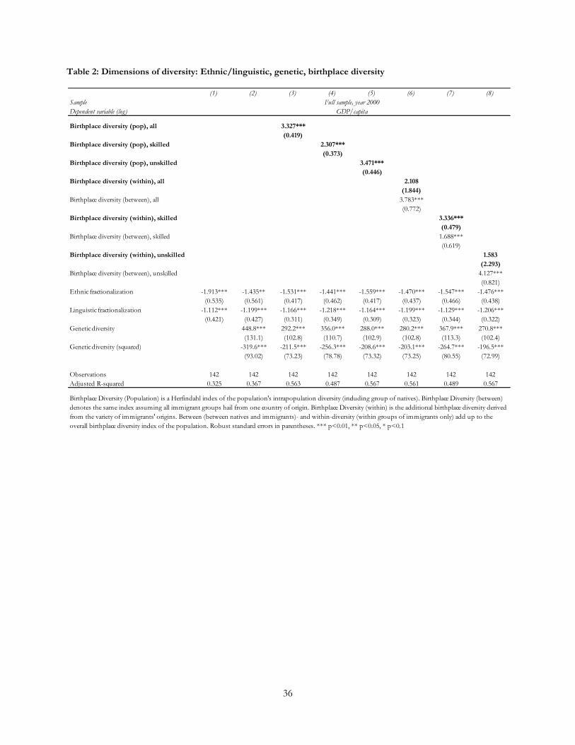
36

Table 2: Dimensions of diversity: Ethnic/linguistic, genetic, birthplace diversity

(1) (2) (3) (4) (5) (6) (7) (8)

Sample

Dependent variable (log)

Birthplace diversity (pop), all 3.327***

(0.419)

Birthplace diversity (pop), skilled 2.307***

(0.373)

Birthplace diversity (pop), unskilled 3.471***

(0.446)

Birthplace diversity (within), all 2.108

(1.844)

Birthplace diversity (between), all 3.783***

(0.772)

Birthplace diversity (within), skilled 3.336***

(0.479)

Birthplace diversity (between), skilled 1.688***

(0.619)

Birthplace diversity (within), unskilled 1.583

(2.293)

Birthplace diversity (between), unskilled 4.127***

(0.821)

Ethnic fractionalization -1.913*** -1.435** -1.531*** -1.441*** -1.559*** -1.470*** -1.547*** -1.476***

(0.535) (0.561) (0.417) (0.462) (0.417) (0.437) (0.466) (0.438)

Linguistic fractionalization -1.112*** -1.199*** -1.166*** -1.218*** -1.164*** -1.199*** -1.129*** -1.206***

(0.421) (0.427) (0.311) (0.349) (0.309) (0.323) (0.344) (0.322)

Genetic diversity 448.8*** 292.2*** 356.0*** 288.0*** 280.2*** 367.9*** 270.8***

(131.1) (102.8) (110.7) (102.9) (102.8) (113.3) (102.4)

Genetic diversity (squared) -319.6*** -211.5*** -256.3*** -208.6*** -203.1*** -264.7*** -196.5***

(93.02) (73.23) (78.78) (73.32) (73.25) (80.55) (72.99)

Observations 142 142 142 142 142 142 142 142

Adjusted R-squared 0.325 0.367 0.563 0.487 0.567 0.561 0.489 0.567

Full sample, year 2000

GDP/capita

Birthplace Diversity (Population) is a Herfindahl index of the population's intrapopulation diversity (including group of natives). Birthplace Diversity (between)

denotes the same index assuming all immigrant groups hail from one country of origin. Birthplace Diversity (within) is the additional birthplace diversity derived

from the variety of immigrants' origins. Between (between natives and immigrants)- and within-diversity (within groups of immigrants only) add up to the

overall birthplace diversity index of the population. Robust standard errors in parentheses. *** p<0.01, ** p<0.05, * p<0.1

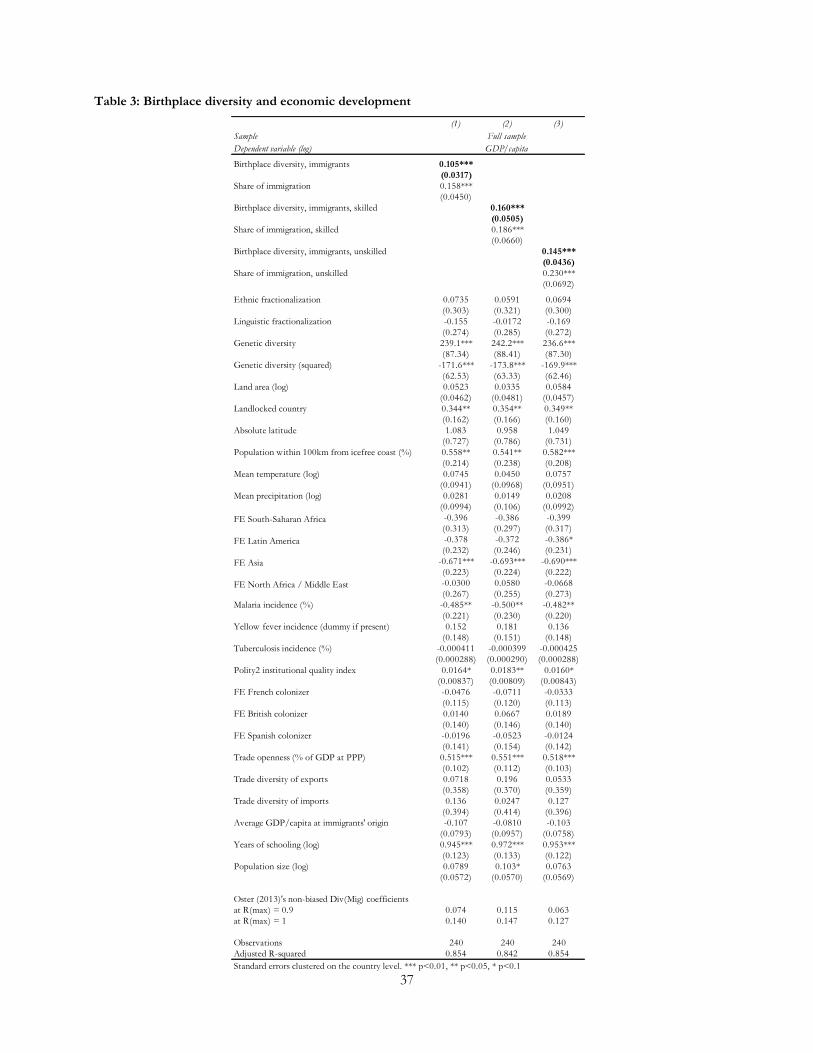
37

Table 3: Birthplace diversity and economic development

(1) (2) (3)

Sample

Dependent variable (log)

Birthplace diversity, immigrants 0.105***

(0.0317)

Share of immigration 0.158***

(0.0450)

Birthplace diversity, immigrants, skilled 0.160***

(0.0505)

Share of immigration, skilled 0.186***

(0.0660)

Birthplace diversity, immigrants, unskilled 0.145***

(0.0436)

Share of immigration, unskilled 0.230***

(0.0692)

Ethnic fractionalization 0.0735 0.0591 0.0694

(0.303) (0.321) (0.300)

Linguistic fractionalization -0.155 -0.0172 -0.169

(0.274) (0.285) (0.272)

Genetic diversity 239.1*** 242.2*** 236.6***

(87.34) (88.41) (87.30)

Genetic diversity (squared) -171.6*** -173.8*** -169.9***

(62.53) (63.33) (62.46)

Land area (log) 0.0523 0.0335 0.0584

(0.0462) (0.0481) (0.0457)

Landlocked country 0.344** 0.354** 0.349**

(0.162) (0.166) (0.160)

Absolute latitude 1.083 0.958 1.049

(0.727) (0.786) (0.731)

Population within 100km from icefree coast (%) 0.558** 0.541** 0.582***

(0.214) (0.238) (0.208)

Mean temperature (log) 0.0745 0.0450 0.0757

(0.0941) (0.0968) (0.0951)

Mean precipitation (log) 0.0281 0.0149 0.0208

(0.0994) (0.106) (0.0992)

FE South-Saharan Africa -0.396 -0.386 -0.399

(0.313) (0.297) (0.317)

FE Latin America -0.378 -0.372 -0.386*

(0.232) (0.246) (0.231)

FE Asia -0.671*** -0.693*** -0.690***

(0.223) (0.224) (0.222)

FE North Africa / Middle East -0.0300 0.0580 -0.0668

(0.267) (0.255) (0.273)

Malaria incidence (%) -0.485** -0.500** -0.482**

(0.221) (0.230) (0.220)

Yellow fever incidence (dummy if present) 0.152 0.181 0.136

(0.148) (0.151) (0.148)

Tuberculosis incidence (%) -0.000411 -0.000399 -0.000425

(0.000288) (0.000290) (0.000288)

Polity2 institutional quality index 0.0164* 0.0183** 0.0160*

(0.00837) (0.00809) (0.00843)

FE French colonizer -0.0476 -0.0711 -0.0333

(0.115) (0.120) (0.113)

FE British colonizer 0.0140 0.0667 0.0189

(0.140) (0.146) (0.140)

FE Spanish colonizer -0.0196 -0.0523 -0.0124

(0.141) (0.154) (0.142)

Trade openness (% of GDP at PPP) 0.515*** 0.551*** 0.518***

(0.102) (0.112) (0.103)

Trade diversity of exports 0.0718 0.196 0.0533

(0.358) (0.370) (0.359)

Trade diversity of imports 0.136 0.0247 0.127

(0.394) (0.414) (0.396)

Average GDP/capita at immigrants' origin -0.107 -0.0810 -0.103

(0.0793) (0.0957) (0.0758)

Years of schooling (log) 0.945*** 0.972*** 0.953***

(0.123) (0.133) (0.122)

Population size (log) 0.0789 0.103* 0.0763

(0.0572) (0.0570) (0.0569)

Oster (2013)'s non-biased Div(Mig) coefficients

at R(max) = 0.9 0.074 0.115 0.063

at R(max) = 1 0.140 0.147 0.127

Observations 240 240 240

Adjusted R-squared 0.854 0.842 0.854

Standard errors clustered on the country level. *** p<0.01, ** p<0.05, * p<0.1

Full sample

GDP/capita

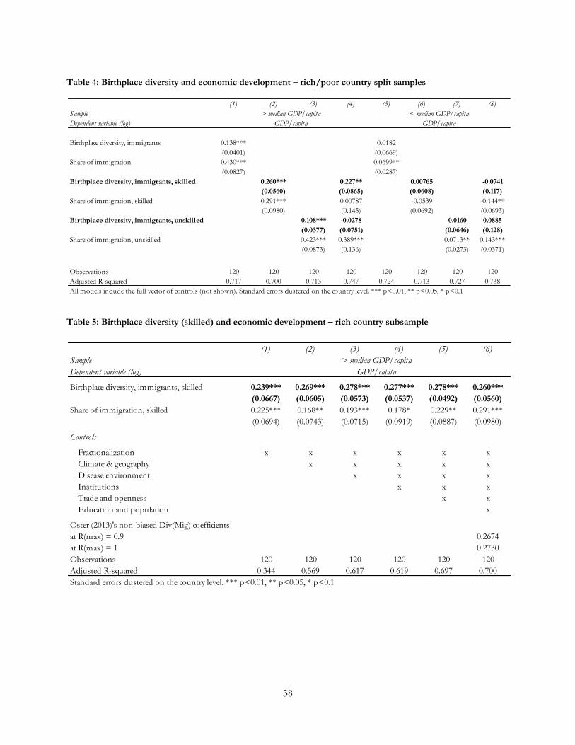
38

Table 4: Birthplace diversity and economic development – rich/poor country split samples

Table 5: Birthplace diversity (skilled) and economic development – rich country subsample

(1) (2) (3) (4) (5) (6) (7) (8)

Sample

Dependent variable (log)

Birthplace diversity, immigrants 0.138*** 0.0182

(0.0401) (0.0669)

Share of immigration 0.430*** 0.0699**

(0.0827) (0.0287)

Birthplace diversity, immigrants, skilled 0.260*** 0.227** 0.00765 -0.0741

(0.0560) (0.0865) (0.0608) (0.117)

Share of immigration, skilled 0.291*** 0.00787 -0.0539 -0.144**

(0.0980) (0.145) (0.0692) (0.0693)

Birthplace diversity, immigrants, unskilled 0.108*** -0.0278 0.0160 0.0885

(0.0377) (0.0751) (0.0646) (0.128)

Share of immigration, unskilled 0.423*** 0.389*** 0.0713** 0.143***

(0.0873) (0.136) (0.0273) (0.0371)

Observations 120 120 120 120 120 120 120 120

Adjusted R-squared 0.717 0.700 0.713 0.747 0.724 0.713 0.727 0.738

> median GDP/capita < median GDP/capita

GDP/capita GDP/capita

All models include the full vector of controls (not shown). Standard errors clustered on the country level. *** p<0.01, ** p<0.05, * p<0.1

(1) (2) (3) (4) (5) (6)

Sample

Dependent variable (log)

Birthplace diversity, immigrants, skilled 0.239*** 0.269*** 0.278*** 0.277*** 0.278*** 0.260***

(0.0667) (0.0605) (0.0573) (0.0537) (0.0492) (0.0560)

Share of immigration, skilled 0.225*** 0.168** 0.193*** 0.178* 0.229** 0.291***

(0.0694) (0.0743) (0.0715) (0.0919) (0.0887) (0.0980)

Controls

Fractionalization x x x x x x

Climate & geography x x x x x

Disease environment x x x x

Institutions x x x

Trade and openness x x

Education and population x

Oster (2013)'s non-biased Div(Mig) coefficients

at R(max) = 0.9 0.2674

at R(max) = 1 0.2730

Observations 120 120 120 120 120 120

Adjusted R-squared 0.344 0.569 0.617 0.619 0.697 0.700

Standard errors clustered on the country level. *** p<0.01, ** p<0.05, * p<0.1

> median GDP/capita

GDP/capita

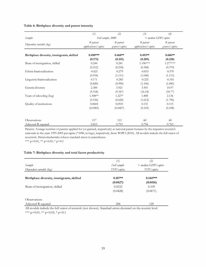
39

Table 6: Birthplace diversity and patent intensity

Table 7: Birthplace diversity and total factor productivity

(1) (2) (3) (4)

Sample

Dependent variable (log)# patent

applications/capita

# patent

grants/capita

# patent

applications/capita

# patent

grants/capita

Birthplace diversity, immigrants, skilled 0.490*** 0.468** 0.493** 0.606**

(0.173) (0.215) (0.205) (0.228)

Share of immigration, skilled 0.244 0.241 1.196*** 1.277***

(0.212) (0.218) (0.368) (0.370)

Ethnic fractionalization -0.621 -0.279 -0.833 -0.570

(0.934) (1.111) (1.040) (1.113)

Linguistic fractionalization 0.171 -0.283 -0.225 -0.316

(0.820) (0.990) (1.106) (1.085)

Genetic diversity 2.300 5.921 3.501 10.97

(9.318) (9.347) (16.18) (18.77)

Years of schooling (log) 1.308** 1.227* 1.808 2.136

(0.536) (0.620) (1.612) (1.796)

Quality of institutions 0.0604 0.0551 0.131 0.115

(0.0383) (0.0407) (0.103) (0.108)

Observations 117 112 60 60

Adjusted R-squared 0.813 0.793 0.794 0.763

*** p<0.01, ** p<0.05, * p<0.1

Patents: Average number of patents applied for (or granted, respectively) at national patent bureaus by the respective country's

nationals in the years 1995-2005 per capita (*1000, in logs), respectively, from WIPO (2010). All models include the full vector of

countrols. Heteroskedasticity-robust standard errors in parentheses.

Full sample, 2000 > median GDP/capita

(1) (2)

Sample Full sample > median GDP/capita

Dependent variable (log) TFP/capita TFP/capita

Birthplace diversity, immigrants, skilled 0.107** 0.144***

(0.0427) (0.0416)

Share of immigration, skilled 0.0232 0.109

(0.0428) (0.0671)

Observations

Adjusted R-squared 206 120

*** p<0.01, ** p<0.05, * p<0.1

All models include the full vector of controls (not shown). Standard errors clustered on the country level.

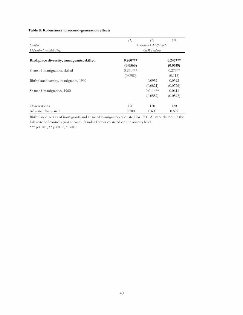
40

Table 8: Robustness to second-generation effects

(1) (2) (3)

Sample

Dependent variable (log)

Birthplace diversity, immigrants, skilled 0.260*** 0.247***

(0.0560) (0.0619)

Share of immigration, skilled 0.291*** 0.273**

(0.0980) (0.115)

Birthplace diversity, immigrants, 1960 0.0952 0.0392

(0.0821) (0.0776)

Share of immigration, 1960 0.0114** 0.0611

(0.0557) (0.0592)

Observations 120 120 120

Adjusted R-squared 0.700 0.600 0.699

*** p<0.01, ** p<0.05, * p<0.1

> median GDP/capita

GDP/capita

Birthplace diversity of immigrants and share of immigration calculated for 1960. All models include the

full vector of controls (not shown). Standard errors clustered on the country level.

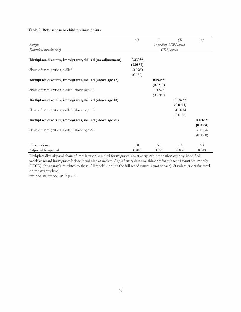
41

Table 9: Robustness to children immigrants

(1) (2) (3) (4)

Sample

Dependent variable (log)

Birthplace diversity, immigrants, skilled (no adjustment) 0.230**

(0.0855)

Share of immigration, skilled -0.0960

(0.189)

Birthplace diversity, immigrants, skilled (above age 12) 0.192**

(0.0710)

Share of immigration, skilled (above age 12) -0.0526

(0.0887)

Birthplace diversity, immigrants, skilled (above age 18) 0.187**

(0.0701)

Share of immigration, skilled (above age 18) -0.0284

(0.0756)

Birthplace diversity, immigrants, skilled (above age 22) 0.186**

(0.0684)

Share of immigration, skilled (above age 22) -0.0134

(0.0668)

Observations 58 58 58 58

Adjusted R-squared 0.848 0.851 0.850 0.849

*** p<0.01, ** p<0.05, * p<0.1

GDP/capita

Birthplace diversity and share of immigration adjusted for migrants' age at entry into destination country. Modified

variables regard immigrants below thresholds as natives. Age-of-entry data available only for subset of countries (mostly

OECD), thus sample restricted to these. All models include the full set of controls (not shown). Standard errors clustered

on the country level.

> median GDP/capita

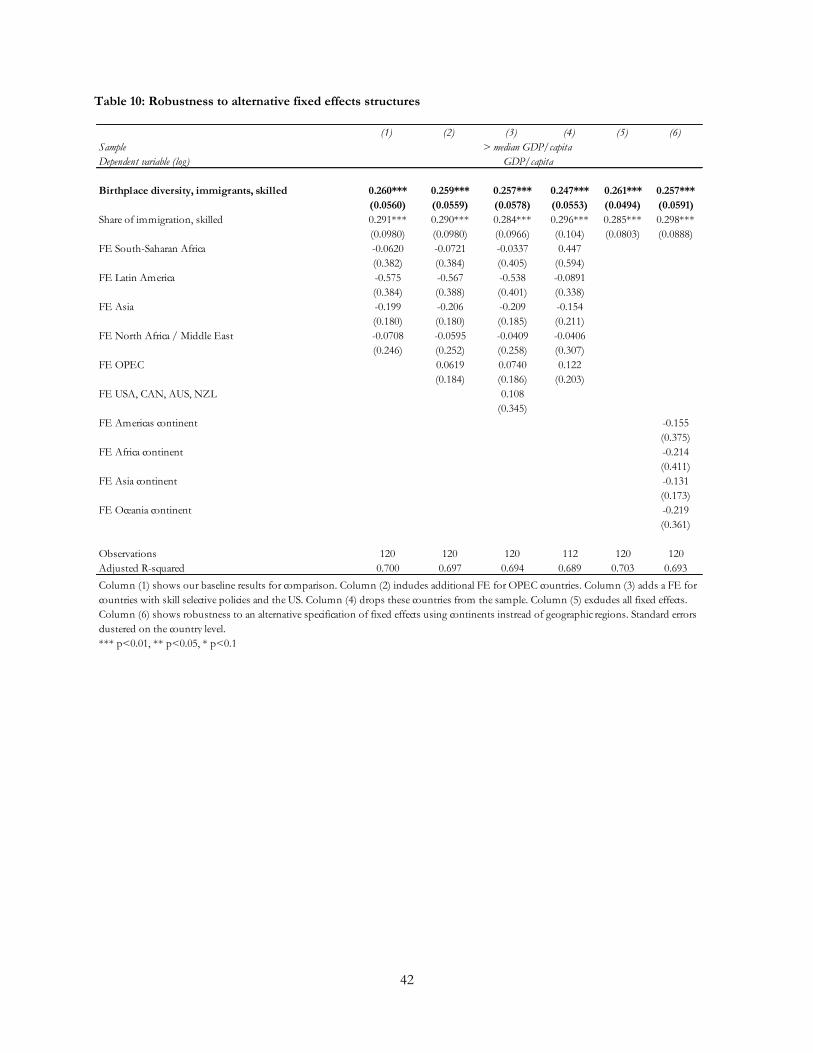
42

Table 10: Robustness to alternative fixed effects structures

(1) (2) (3) (4) (5) (6)

Sample

Dependent variable (log)

Birthplace diversity, immigrants, skilled 0.260*** 0.259*** 0.257*** 0.247*** 0.261*** 0.257***

(0.0560) (0.0559) (0.0578) (0.0553) (0.0494) (0.0591)

Share of immigration, skilled 0.291*** 0.290*** 0.284*** 0.296*** 0.285*** 0.298***

(0.0980) (0.0980) (0.0966) (0.104) (0.0803) (0.0888)

FE South-Saharan Africa -0.0620 -0.0721 -0.0337 0.447

(0.382) (0.384) (0.405) (0.594)

FE Latin America -0.575 -0.567 -0.538 -0.0891

(0.384) (0.388) (0.401) (0.338)

FE Asia -0.199 -0.206 -0.209 -0.154

(0.180) (0.180) (0.185) (0.211)

FE North Africa / Middle East -0.0708 -0.0595 -0.0409 -0.0406

(0.246) (0.252) (0.258) (0.307)

FE OPEC 0.0619 0.0740 0.122

(0.184) (0.186) (0.203)

FE USA, CAN, AUS, NZL 0.108

(0.345)

FE Americas continent -0.155

(0.375)

FE Africa continent -0.214

(0.411)

FE Asia continent -0.131

(0.173)

FE Oceania continent -0.219

(0.361)

Observations 120 120 120 112 120 120

Adjusted R-squared 0.700 0.697 0.694 0.689 0.703 0.693

*** p<0.01, ** p<0.05, * p<0.1

GDP/capita

> median GDP/capita

Column (1) shows our baseline results for comparison. Column (2) includes additional FE for OPEC countries. Column (3) adds a FE for

countries with skill selective policies and the US. Column (4) drops these countries from the sample. Column (5) excludes all fixed effects.

Column (6) shows robustness to an alternative specification of fixed effects using continents instread of geographic regions. Standard errors

clustered on the country level.

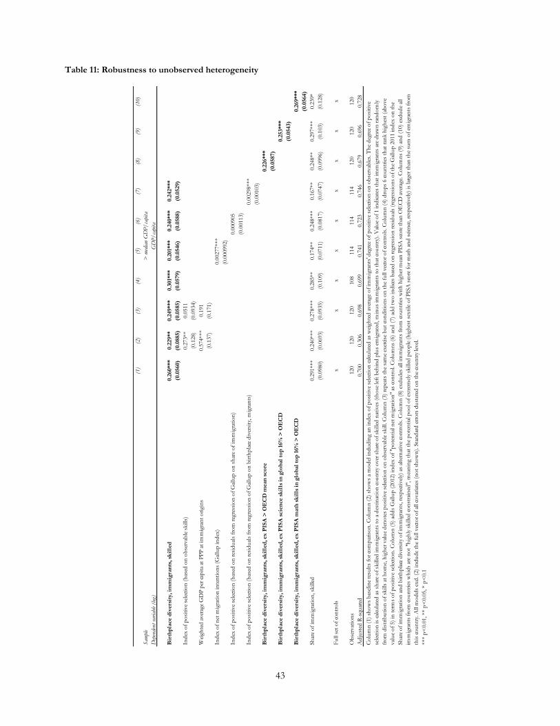
43

Table 11: Robustness to unobserved heterogeneity

(1)

(2)

(3)

(4)

(5)

(6)

(7)

(8)

(9)

(10)

Sam

ple

Dep

ende

nt

vari

able

(lo

g)

Bir

thp

lace d

ivers

ity, im

mig

ran

ts, sk

ille

d0.2

60***

0.2

29**

0.2

49***

0.3

01*

**

0.2

01*

**

0.2

40***

0.2

42***

(0.0

560)

(0.0

885)

(0.0

585)

(0.0

579)

(0.0

546)

(0.0

588)

(0.0

529)

Ind

ex o

f p

osi

tive

sele

ctio

n (

bas

ed o

n o

bse

rvab

le s

kills

)0.2

73**

0.0

511

(0.1

28)

(0.0

934)

Wei

gh

ted

aver

age

GD

P p

er c

apit

a at

PP

P a

t im

mig

ran

t o

rigin

s0.5

74***

0.1

91

(0.1

37)

(0.1

71)

Ind

ex o

f n

et m

igra

tio

n in

ten

tio

ns

(Gal

lup

in

dex

)0.0

0277***

(0.0

00992)

Ind

ex o

f p

osi

tive

sele

ctio

n (

bas

ed o

n r

esid

ual

s fr

om

reg

ress

ion

of

Gal

lup

on

sh

are

of

imm

igra

tio

n)

0.0

00905

(0.0

0113)

Ind

ex o

f p

osi

tive

sele

ctio

n (

bas

ed o

n r

esid

ual

s fr

om

reg

ress

ion

of

Gal

lup

on

bir

thp

lace

div

ersi

ty, m

igra

nts

)0.0

0298***

(0.0

0103)

Bir

thp

lace d

ivers

ity, im

mig

ran

ts, sk

ille

d, ex

PIS

A >

OE

CD

mean

sco

re0.2

26***

(0.0

587)

Bir

thp

lace d

ivers

ity, im

mig

ran

ts, sk

ille

d, ex

PIS

A s

cie

nce s

kil

ls i

n g

lob

al

top

16%

> O

EC

D0.2

53***

(0.0

543)

Bir

thp

lace d

ivers

ity, im

mig

ran

ts, sk

ille

d, ex

PIS

A m

ath

sk

ills

in

glo

bal

top

16%

> O

EC

D0.2

69***

(0.0

564)

Sh

are

of

imm

igra

tio

n, sk

ille

d0.2

91***

0.2

40***

0.2

78***

0.2

85**

0.1

74**

0.2

48***

0.1

67**

0.2

48**

0.2

97***

0.2

39*

(0.0

980)

(0.0

693)

(0.0

935)

(0.1

09)

(0.0

711)

(0.0

817)

(0.0

747)

(0.0

996)

(0.1

03)

(0.1

28)

Fu

ll s

et o

f co

ntr

ols

xx

xx

xx

xx

x

Ob

serv

atio

ns

120

120

120

108

114

114

114

120

120

120

Ad

just

ed R

-squ

ared

0.7

00

0.3

06

0.6

98

0.6

99

0.7

41

0.7

23

0.7

46

0.6

79

0.6

96

0.7

28

*** p

<0.0

1, ** p

<0.0

5, * p

<0.1

Co

lum

n (

1)

sho

ws

bas

elin

e re

sult

s fo

r co

mp

aris

on

. C

olu

mn

(2)

sho

ws

a m

od

el in

clu

din

g a

n in

dex

of

po

siti

ve

sele

ctio

n c

alcu

late

d a

s w

eigh

ted

aver

age

of

imm

igra

nts

' deg

ree

of

po

siti

ve

sele

ctio

n o

n o

bse

rvab

les.

Th

e d

egre

e o

f p

osi

tive

sele

ctio

n is

calc

ula

ted

as

shar

e o

f sk

ille

d im

mig

ran

ts t

o a

des

tin

atio

n c

ou

ntr

y o

ver

sh

are

of

skille

d n

ativ

es (

tho

se lef

t b

ehin

d p

lus

emig

rate

d, m

inu

s im

mig

ran

ts t

o t

hat

co

un

try)

. V

alu

e o

f 1 in

dic

ates

th

at im

mig

ran

ts a

re d

raw

n r

and

om

ly

fro

m d

istr

ibu

tio

n o

f sk

ills

at

ho

me,

hig

her

val

ue

den

ote

s p

osi

tive

sele

ctio

n o

n o

bse

rvab

le s

kill. C

olu

mn

(3)

rep

eats

th

e sa

me

exer

cise

bu

t co

nd

itio

ns

on

th

e fu

ll v

ecto

r o

f co

ntr

ols

. C

olu

mn

(4)

dro

ps

6 c

ou

ntr

ies

that

ran

k h

igh

est

(ab

ove

val

ue

of

5)

in t

erm

s o

f p

osi

tive

sele

ctio

n. C

olu

mn

(5)

add

s G

allu

p (

2012)

ind

ex o

f "p

ote

nti

al n

et m

igra

tio

n"

as c

on

tro

l. C

olu

mn

s (6

) an

d (

7)

add

tw

o in

dic

es b

ased

on

reg

ress

ion

res

idu

als

(reg

ress

ion

s o

f th

e G

allu

p 2

011 in

dex

on

th

e

Sh

are

of

imm

igra

tio

n a

nd

bir

thp

lace

div

ersi

ty o

f im

mig

ran

ts, re

spec

tivel

y) a

s al

tern

ativ

e co

ntr

ols

. C

olu

mn

(8)

excl

ud

es a

ll im

mig

ran

ts f

rom

co

un

trie

s w

ith

hig

her

mea

n P

ISA

sco

re t

han

OE

CD

aver

age.

Co

lum

ns

(9)

and

(10)

excl

ud

e al

l

imm

igra

nts

fro

m c

ou

ntr

ies

wh

ich

are

no

t "h

igh

ly s

kille

d c

on

stra

ined

", m

ean

ing t

hat

th

e p

ote

nti

al p

oo

l o

f ex

trem

ely

skille

d p

eop

le (

hig

hes

t se

xti

le o

f P

ISA

sco

re f

or

mat

h a

nd

sci

ence

, re

spec

tivel

y) is

larg

er t

han

th

e su

m o

f em

igra

nts

fro

m

this

co

un

try.

All m

od

els

excl

. (2

) in

clu

de

the

full v

ecto

r o

f al

l co

var

iate

s (n

ot

sho

wn

). S

tan

dar

d e

rro

rs c

lust

ered

on

th

e co

un

try

level

.

> m

edia

n G

DP

/ca

pita

GD

P/

capi

ta

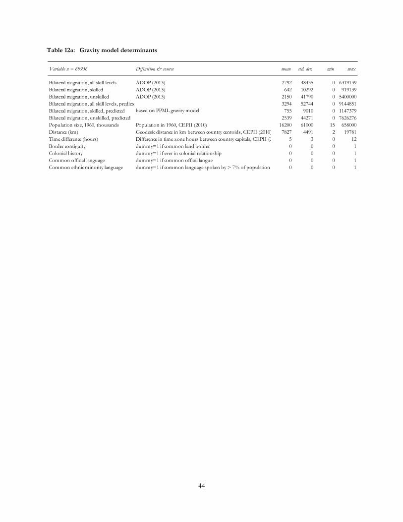
44

Table 12a: Gravity model determinants

Variable n = 69936 Def inition & source mean std. dev. min max

Bilateral migration, all skill levels ADOP (2013) 2792 48435 0 6319139

Bilateral migration, skilled ADOP (2013) 642 10292 0 919139

Bilateral migration, unskilled ADOP (2013) 2150 41790 0 5400000

Bilateral migration, all skill levels, predicted 3294 52744 0 9144851

Bilateral migration, skilled, predicted 755 9010 0 1147379

Bilateral migration, unskilled, predicted 2539 44271 0 7626276

Population size, 1960, thousands Population in 1960, CEPII (2010) 16200 61000 15 658000

Distance (km) Geodesic distance in km between country centoids, CEPII (2010) 7827 4491 2 19781

Time difference (hours) Difference in time zone hours between country capitals, CEPII (2010) 5 3 0 12

Border contiguity dummy=1 if common land border 0 0 0 1

Colonial history dummy=1 if ever in colonial relationship 0 0 0 1

Common official language dummy=1 if common offical langue 0 0 0 1

Common ethnic minority language dummy=1 if common language spoken by > 7% of population 0 0 0 1

based on PPML gravity model

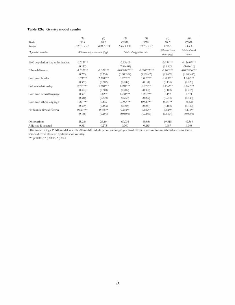
45

Table 12b: Gravity model results

(1) (2) (3) (4) (5) (6)

Model OLS OLS PPML PPML OLS PPML

Sample SKILLED SKILLED SKILLED SKILLED FULL FULL

Dependent variableBilateral trade

share (log)

Bilateral trade

share

1960 population size at destination -0.313*** -6.95e-09 -0.194*** 4.11e-09***

(0.112) (7.59e-09) (0.0503) (9.64e-10)

Bilateral distance -1.332*** -1.322*** -0.000342*** -0.000323*** -1.060*** -0.002696***

(0.233) (0.235) (0.000104) (9.82e-05) (0.0669) (0.000485)

Common border 0.796** 2.368*** 0.973*** 1.007*** 0.983*** 1.942***

(0.367) (0.307) (0.242) (0.178) (0.130) (0.228)

Colonial relationship 2.767*** 1.260*** 1.091*** 0.772** 1.156*** 0.660***

(0.424) (0.369) (0.209) (0.322) (0.103) (0.216)

Common official language 0.371 0.628* 1.234*** 1.287*** 0.192 0.571

(0.340) (0.349) (0.258) (0.272) (0.210) (0.548)

Common ethnic language 1.297*** 0.436 0.799*** 0.926*** 0.357** -0.228

(0.379) (0.455) (0.308) (0.247) (0.160) (0.332)

Horizontal time difference 0.523*** 0.465** 0.218** 0.189** 0.0259 0.175**

(0.188) (0.191) (0.0895) (0.0809) (0.0594) (0.0790)

Observations 25,244 25,244 69,936 69,936 19,315 42,369

Adjusted R-squared 0.311 0.275 0.300 0.285 0.687 0.308

*** p<0.01, ** p<0.05, * p<0.1

Bilateral migration rate (log) Bilateral migration rate

OLS model in logs, PPML model in levels. All models include period and origin-year fixed effects to account for multilateral resistance terms.

Standard errors clustered by destination country.

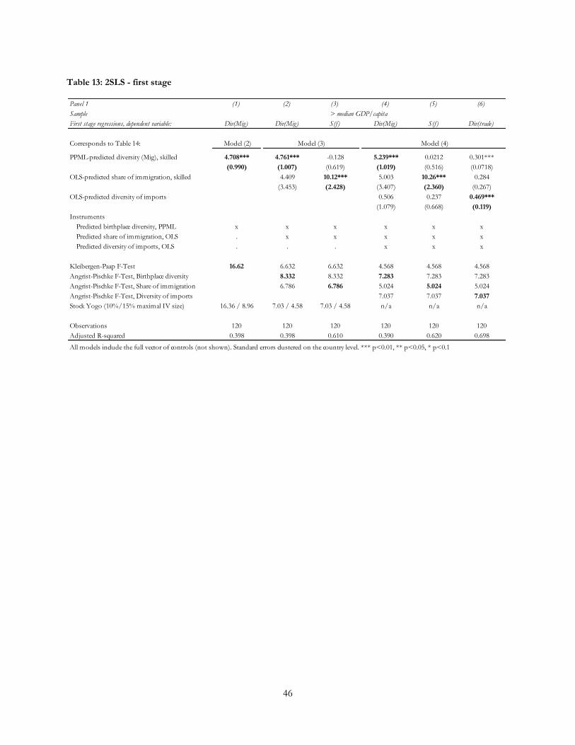
46

Table 13: 2SLS - first stage

Panel 1 (1) (2) (3) (4) (5) (6)

Sample

First stage regressions, dependent variable: Div(Mig) Div(Mig) S(f ) Div(Mig) S(f ) Div(trade)

Corresponds to Table 14: Model (2)

PPML-predicted diversity (Mig), skilled 4.708*** 4.761*** -0.128 5.239*** 0.0212 0.301***

(0.990) (1.007) (0.619) (1.019) (0.516) (0.0718)

OLS-predicted share of immigration, skilled 4.409 10.12*** 5.003 10.26*** 0.284

(3.453) (2.428) (3.407) (2.360) (0.267)

OLS-predicted diversity of imports 0.506 0.237 0.469***

(1.079) (0.668) (0.119)

Instruments

Predicted birthplace diversity, PPML x x x x x x

Predicted share of immigration, OLS . x x x x x

Predicted diversity of imports, OLS . . . x x x

Kleibergen-Paap F-Test 16.62 6.632 6.632 4.568 4.568 4.568

Angrist-Pischke F-Test, Birthplace diversity 8.332 8.332 7.283 7.283 7.283

Angrist-Pischke F-Test, Share of immigration 6.786 6.786 5.024 5.024 5.024

Angrist-Pischke F-Test, Diversity of imports 7.037 7.037 7.037

Stock Yogo (10%/15% maximal IV size) 16.36 / 8.96 7.03 / 4.58 7.03 / 4.58 n/a n/a n/a

Observations 120 120 120 120 120 120

Adjusted R-squared 0.398 0.398 0.610 0.390 0.620 0.698

> median GDP/capita

Model (3) Model (4)

All models include the full vector of controls (not shown). Standard errors clustered on the country level. *** p<0.01, ** p<0.05, * p<0.1

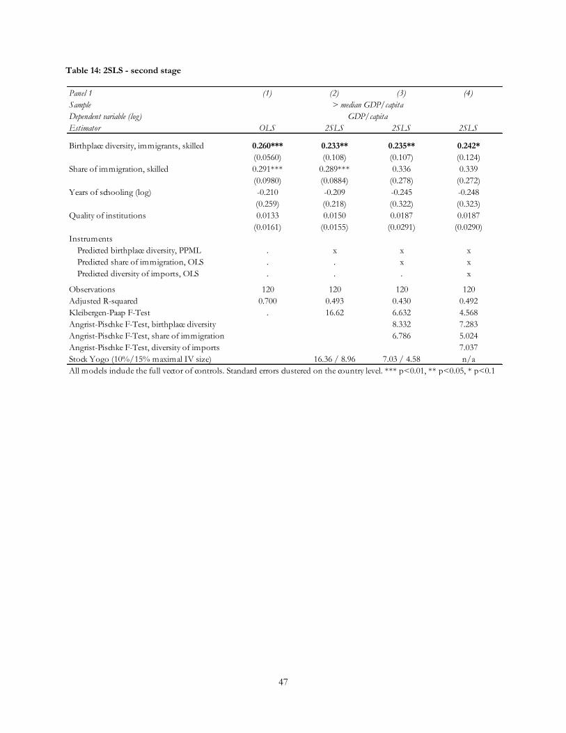
47

Table 14: 2SLS - second stage

Panel 1 (1) (2) (3) (4)

Sample

Dependent variable (log)

Estimator OLS 2SLS 2SLS 2SLS

Birthplace diversity, immigrants, skilled 0.260*** 0.233** 0.235** 0.242*

(0.0560) (0.108) (0.107) (0.124)

Share of immigration, skilled 0.291*** 0.289*** 0.336 0.339

(0.0980) (0.0884) (0.278) (0.272)

Years of schooling (log) -0.210 -0.209 -0.245 -0.248

(0.259) (0.218) (0.322) (0.323)

Quality of institutions 0.0133 0.0150 0.0187 0.0187

(0.0161) (0.0155) (0.0291) (0.0290)

Instruments

Predicted birthplace diversity, PPML . x x x

Predicted share of immigration, OLS . . x x

Predicted diversity of imports, OLS . . . x

Observations 120 120 120 120

Adjusted R-squared 0.700 0.493 0.430 0.492

Kleibergen-Paap F-Test . 16.62 6.632 4.568

Angrist-Pischke F-Test, birthplace diversity 8.332 7.283

Angrist-Pischke F-Test, share of immigration 6.786 5.024

Angrist-Pischke F-Test, diversity of imports 7.037

Stock Yogo (10%/15% maximal IV size) 16.36 / 8.96 7.03 / 4.58 n/a

> median GDP/capita

GDP/capita

All models include the full vector of controls. Standard errors clustered on the country level. *** p<0.01, ** p<0.05, * p<0.1

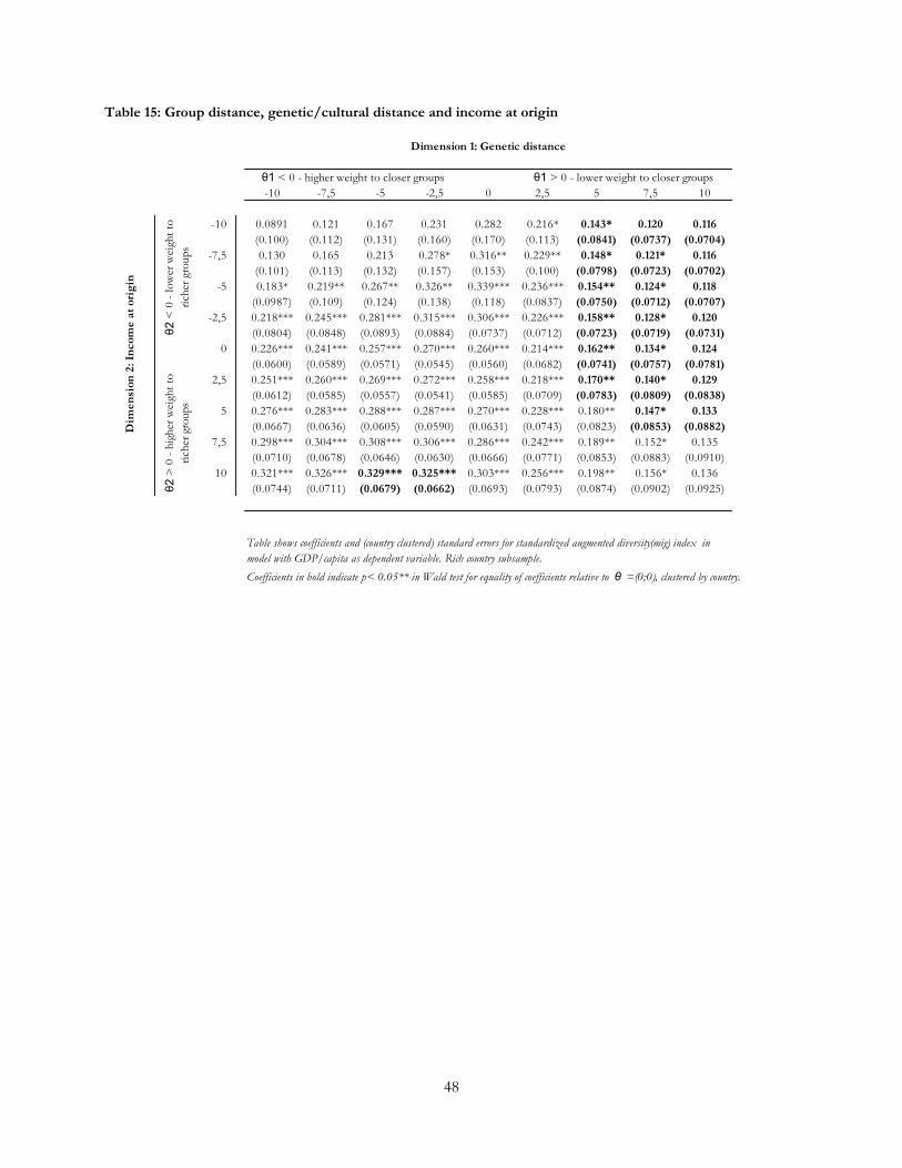
48

Table 15: Group distance, genetic/cultural distance and income at origin

-10 -7,5 -5 -2,5 0 2,5 5 7,5 10

-10 0.0891 0.121 0.167 0.231 0.282 0.216* 0.143* 0.120 0.116

(0.100) (0.112) (0.131) (0.160) (0.170) (0.113) (0.0841) (0.0737) (0.0704)

-7,5 0.130 0.165 0.213 0.278* 0.316** 0.229** 0.148* 0.121* 0.116

(0.101) (0.113) (0.132) (0.157) (0.153) (0.100) (0.0798) (0.0723) (0.0702)

-5 0.183* 0.219** 0.267** 0.326** 0.339*** 0.236*** 0.154** 0.124* 0.118

(0.0987) (0.109) (0.124) (0.138) (0.118) (0.0837) (0.0750) (0.0712) (0.0707)

-2,5 0.218*** 0.245*** 0.281*** 0.315*** 0.306*** 0.226*** 0.158** 0.128* 0.120

(0.0804) (0.0848) (0.0893) (0.0884) (0.0737) (0.0712) (0.0723) (0.0719) (0.0731)

0 0.226*** 0.241*** 0.257*** 0.270*** 0.260*** 0.214*** 0.162** 0.134* 0.124

(0.0600) (0.0589) (0.0571) (0.0545) (0.0560) (0.0682) (0.0741) (0.0757) (0.0781)

2,5 0.251*** 0.260*** 0.269*** 0.272*** 0.258*** 0.218*** 0.170** 0.140* 0.129

(0.0612) (0.0585) (0.0557) (0.0541) (0.0585) (0.0709) (0.0783) (0.0809) (0.0838)

5 0.276*** 0.283*** 0.288*** 0.287*** 0.270*** 0.228*** 0.180** 0.147* 0.133

(0.0667) (0.0636) (0.0605) (0.0590) (0.0631) (0.0743) (0.0823) (0.0853) (0.0882)

7,5 0.298*** 0.304*** 0.308*** 0.306*** 0.286*** 0.242*** 0.189** 0.152* 0.135

(0.0710) (0.0678) (0.0646) (0.0630) (0.0666) (0.0771) (0.0853) (0.0883) (0.0910)

10 0.321*** 0.326*** 0.329*** 0.325*** 0.303*** 0.256*** 0.198** 0.156* 0.136

(0.0744) (0.0711) (0.0679) (0.0662) (0.0693) (0.0793) (0.0874) (0.0902) (0.0925)

Coefficients in bold indicate p< 0.05** in Wald test for equality of coefficients relative to θ =(0;0), clustered by country.

Table shows coefficients and (country clustered) standard errors for standardized augmented diversity(mig) index in

model with GDP/capita as dependent variable. Rich country subsample.

Dimension 1: Genetic distance

θ1 < 0 - higher weight to closer groups θ1 > 0 - lower weight to closer groups

Dim

en

sion

2: In

com

e a

t ori

gin

θ2 <

0 -

low

er w

eigh

t to

rich

er g

roups

θ2 >

0 -

hig

her

wei

ght

to

rich

er g

roups

Appendix – 1

ONLINE APPENDIX

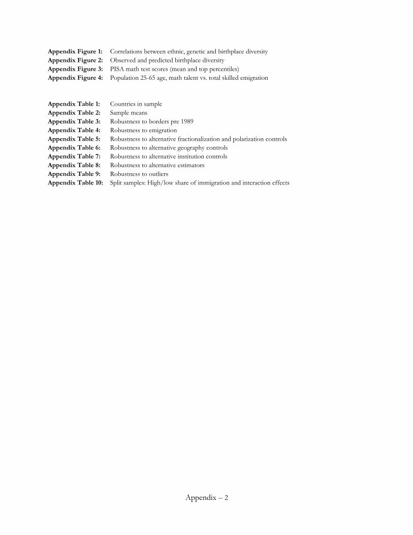
Appendix – 2

Appendix Figure 1: Correlations between ethnic, genetic and birthplace diversity Appendix Figure 2: Observed and predicted birthplace diversity Appendix Figure 3: PISA math test scores (mean and top percentiles)

Appendix Figure 4: Population 25-65 age, math talent vs. total skilled emigration

Appendix Table 1: Countries in sample

Appendix Table 2: Sample means

Appendix Table 3: Robustness to borders pre 1989

Appendix Table 4: Robustness to emigration

Appendix Table 5: Robustness to alternative fractionalization and polarization controls

Appendix Table 6: Robustness to alternative geography controls

Appendix Table 7: Robustness to alternative institution controls

Appendix Table 8: Robustness to alternative estimators

Appendix Table 9: Robustness to outliers

Appendix Table 10: Split samples: High/low share of immigration and interaction effects

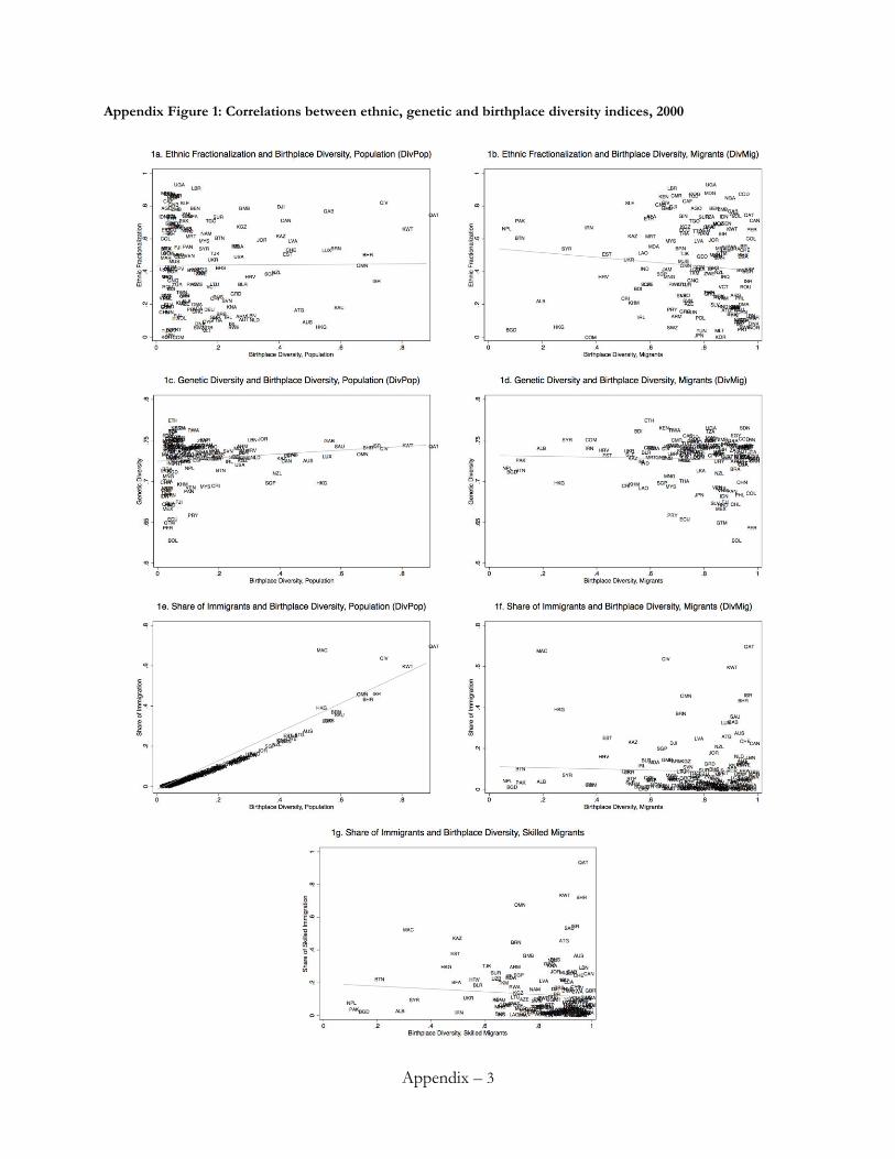
Appendix – 3

Appendix Figure 1: Correlations between ethnic, genetic and birthplace diversity indices, 2000

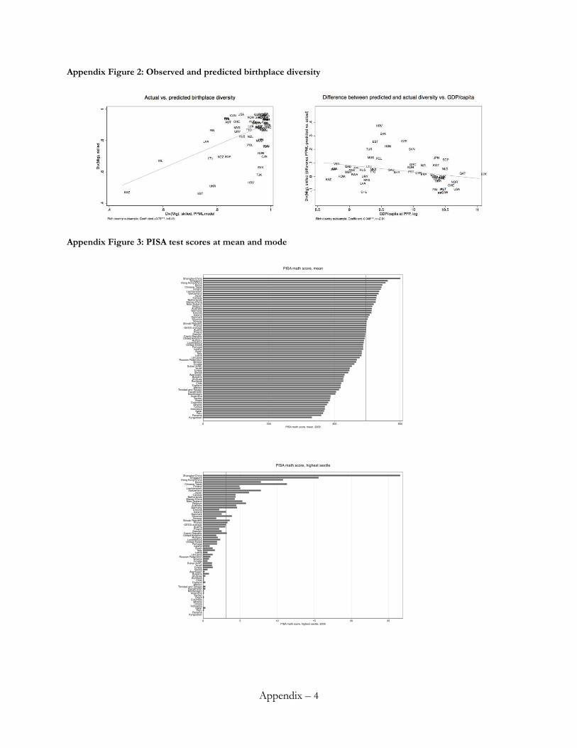
Appendix – 4

Appendix Figure 2: Observed and predicted birthplace diversity

Appendix Figure 3: PISA test scores at mean and mode

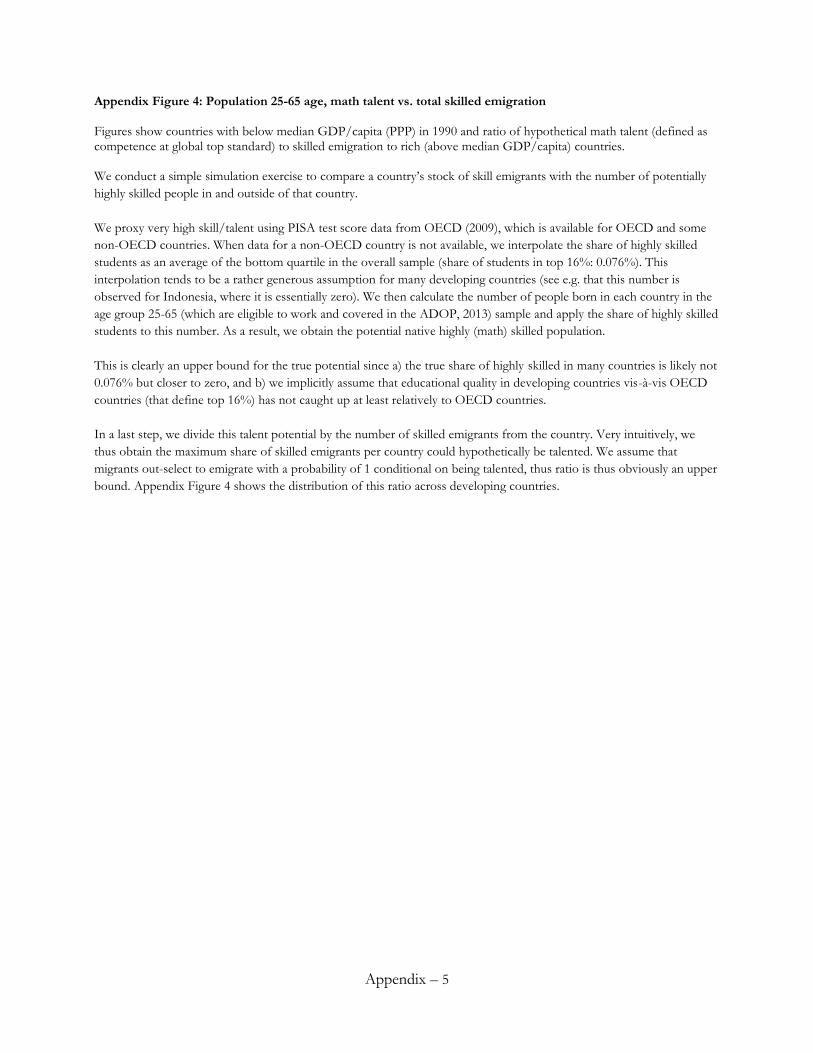
Appendix – 5

Appendix Figure 4: Population 25-65 age, math talent vs. total skilled emigration Figures show countries with below median GDP/capita (PPP) in 1990 and ratio of hypothetical math talent (defined as competence at global top standard) to skilled emigration to rich (above median GDP/capita) countries. We conduct a simple simulation exercise to compare a country’s stock of skill emigrants with the number of potentially

highly skilled people in and outside of that country.

We proxy very high skill/talent using PISA test score data from OECD (2009), which is available for OECD and some

non-OECD countries. When data for a non-OECD country is not available, we interpolate the share of highly skilled

students as an average of the bottom quartile in the overall sample (share of students in top 16%: 0.076%). This

interpolation tends to be a rather generous assumption for many developing countries (see e.g. that this number is

observed for Indonesia, where it is essentially zero). We then calculate the number of people born in each country in the

age group 25-65 (which are eligible to work and covered in the ADOP, 2013) sample and apply the share of highly skilled

students to this number. As a result, we obtain the potential native highly (math) skilled population.

This is clearly an upper bound for the true potential since a) the true share of highly skilled in many countries is likely not

0.076% but closer to zero, and b) we implicitly assume that educational quality in developing countries vis-à-vis OECD

countries (that define top 16%) has not caught up at least relatively to OECD countries.

In a last step, we divide this talent potential by the number of skilled emigrants from the country. Very intuitively, we

thus obtain the maximum share of skilled emigrants per country could hypothetically be talented. We assume that

migrants out-select to emigrate with a probability of 1 conditional on being talented, thus ratio is thus obviously an upper

bound. Appendix Figure 4 shows the distribution of this ratio across developing countries.

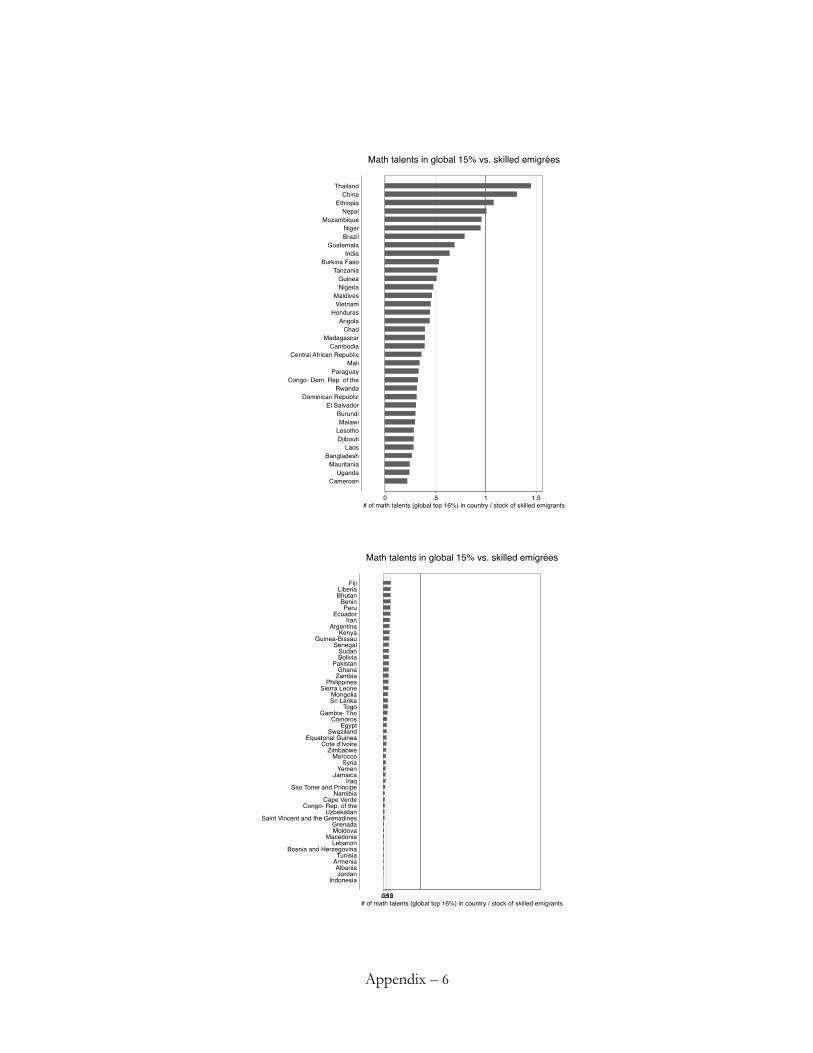
Appendix – 6

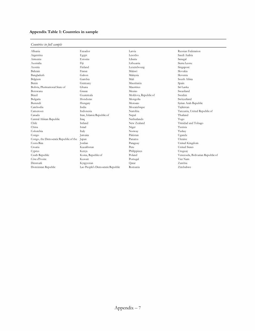
Appendix – 7

Appendix Table 1: Countries in sample

Countries in full sample

Albania Ecuador Latvia Russian Federation

Argentina Egypt Lesotho Saudi Arabia

Armenia Estonia Liberia Senegal

Australia Fiji Lithuania Sierra Leone

Austria Finland Luxembourg Singapore

Bahrain France Malawi Slovakia

Bangladesh Gabon Malaysia Slovenia

Belgium Gambia Mali South Africa

Benin Germany Mauritania Spain

Bolivia, Plurinational State of Ghana Mauritius Sri Lanka

Botswana Greece Mexico Swaziland

Brazil Guatemala Moldova, Republic of Sweden

Bulgaria Honduras Mongolia Switzerland

Burundi Hungary Morocco Syrian Arab Republic

Cambodia India Mozambique Tajikistan

Cameroon Indonesia Namibia Tanzania, United Republic of

Canada Iran, Islamic Republic of Nepal Thailand

Central African Republic Iraq Netherlands Togo

Chile Ireland New Zealand Trinidad and Tobago

China Israel Niger Tunisia

Colombia Italy Norway Turkey

Congo Jamaica Pakistan Uganda

Congo, the Democratic Republic of the Japan Panama Ukraine

Costa Rica Jordan Paraguay United Kingdom

Croatia Kazakhstan Peru United States

Cyprus Kenya Philippines Uruguay

Czech Republic Korea, Republic of Poland Venezuela, Bolivarian Republic of

Côte d'Ivoire Kuwait Portugal Viet Nam

Denmark Kyrgyzstan Qatar Zambia

Dominican Republic Lao People's Democratic Republic Romania Zimbabwe

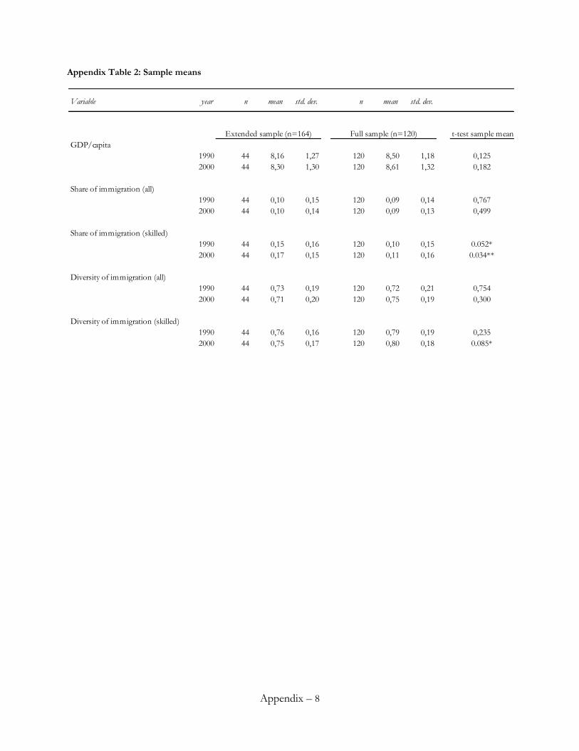
Appendix – 8

Appendix Table 2: Sample means

Variable year n mean std. dev. n mean std. dev.

t-test sample means

GDP/capita

1990 44 8,16 1,27 120 8,50 1,18 0,125

2000 44 8,30 1,30 120 8,61 1,32 0,182

Share of immigration (all)

1990 44 0,10 0,15 120 0,09 0,14 0,767

2000 44 0,10 0,14 120 0,09 0,13 0,499

Share of immigration (skilled)

1990 44 0,15 0,16 120 0,10 0,15 0.052*

2000 44 0,17 0,15 120 0,11 0,16 0.034**

Diversity of immigration (all)

1990 44 0,73 0,19 120 0,72 0,21 0,754

2000 44 0,71 0,20 120 0,75 0,19 0,300

Diversity of immigration (skilled)

1990 44 0,76 0,16 120 0,79 0,19 0,235

2000 44 0,75 0,17 120 0,80 0,18 0.085*

Extended sample (n=164) Full sample (n=120)

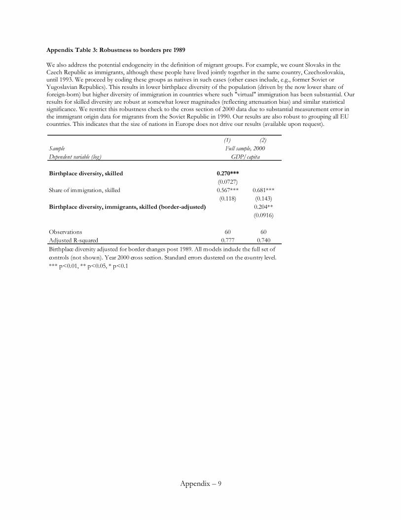
Appendix – 9

Appendix Table 3: Robustness to borders pre 1989 We also address the potential endogeneity in the definition of migrant groups. For example, we count Slovaks in the Czech Republic as immigrants, although these people have lived jointly together in the same country, Czechoslovakia, until 1993. We proceed by coding these groups as natives in such cases (other cases include, e.g., former Soviet or Yugoslavian Republics). This results in lower birthplace diversity of the population (driven by the now lower share of foreign-born) but higher diversity of immigration in countries where such "virtual" immigration has been substantial. Our results for skilled diversity are robust at somewhat lower magnitudes (reflecting attenuation bias) and similar statistical significance. We restrict this robustness check to the cross section of 2000 data due to substantial measurement error in the immigrant origin data for migrants from the Soviet Republic in 1990. Our results are also robust to grouping all EU countries. This indicates that the size of nations in Europe does not drive our results (available upon request).

(1) (2)

Sample

Dependent variable (log)

Birthplace diversity, skilled 0.270***

(0.0727)

Share of immigration, skilled 0.567*** 0.681***

(0.118) (0.143)

Birthplace diversity, immigrants, skilled (border-adjusted) 0.204**

(0.0916)

Observations 60 60

Adjusted R-squared 0.777 0.740

*** p<0.01, ** p<0.05, * p<0.1

Birthplace diversity adjusted for border changes post 1989. All models include the full set of

controls (not shown). Year 2000 cross section. Standard errors clustered on the country level.

Full sample, 2000

GDP/capita

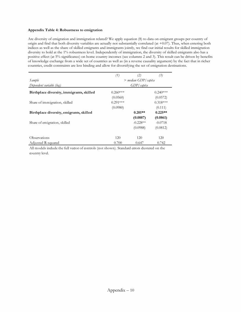
Appendix – 10

Appendix Table 4: Robustness to emigration Are diversity of emigration and immigration related? We apply equation (8) to data on emigrant groups per country of origin and find that both diversity variables are actually not substantially correlated (at +0.07). Thus, when entering both indices as well as the share of skilled emigrants and immigrants jointly, we find our initial results for skilled immigration diversity to hold at the 1% robustness level. Independently of immigration, the diversity of skilled emigrants also has a positive effect (at 5% significance) on home country incomes (see columns 2 and 3). This result can be driven by benefits of knowledge exchange from a wide set of countries as well as (in a reverse causality argument) by the fact that in richer countries, credit constraints are less binding and allow for diversifying the set of emigration destinations.

(1) (2) (3)

Sample

Dependent variable (log)

Birthplace diversity, immigrants, skilled 0.260*** 0.240***

(0.0560) (0.0572)

Share of immigration, skilled 0.291*** 0.318***

(0.0980) (0.111)

Birthplace diversity, emigrants, skilled 0.201** 0.225**

(0.0887) (0.0861)

Share of emigration, skilled -0.228** -0.0718

(0.0988) (0.0812)

Observations 120 120 120

Adjusted R-squared 0.700 0.647 0.742

> median GDP/capita

GDP/capita

All models include the full vector of controls (not shown). Standard errors clustered on the

country level.

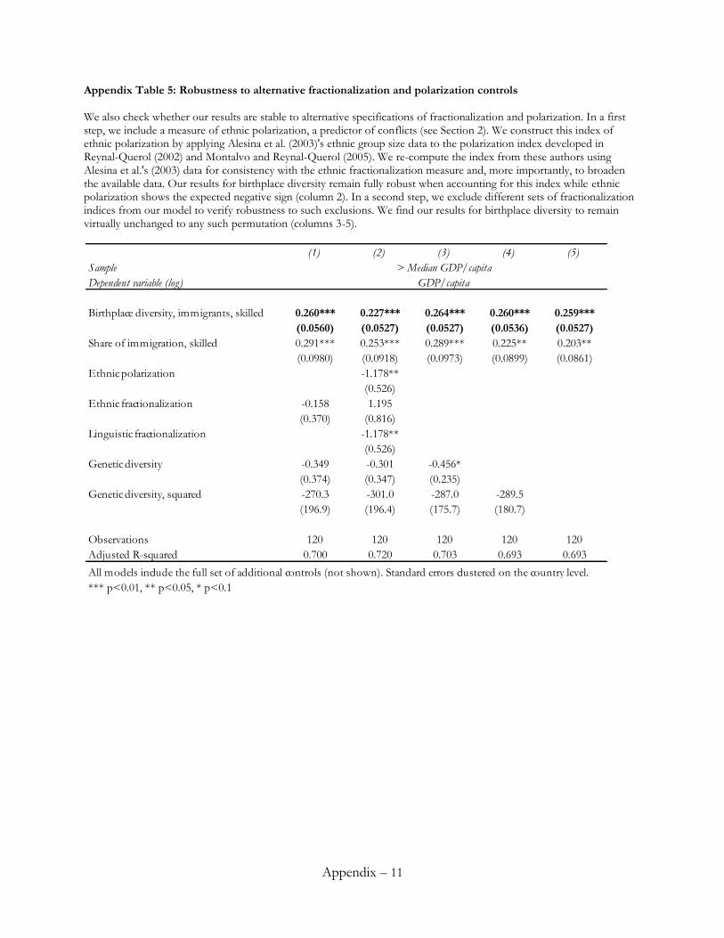
Appendix – 11

Appendix Table 5: Robustness to alternative fractionalization and polarization controls We also check whether our results are stable to alternative specifications of fractionalization and polarization. In a first step, we include a measure of ethnic polarization, a predictor of conflicts (see Section 2). We construct this index of ethnic polarization by applying Alesina et al. (2003)'s ethnic group size data to the polarization index developed in Reynal-Querol (2002) and Montalvo and Reynal-Querol (2005). We re-compute the index from these authors using Alesina et al.'s (2003) data for consistency with the ethnic fractionalization measure and, more importantly, to broaden the available data. Our results for birthplace diversity remain fully robust when accounting for this index while ethnic polarization shows the expected negative sign (column 2). In a second step, we exclude different sets of fractionalization indices from our model to verify robustness to such exclusions. We find our results for birthplace diversity to remain virtually unchanged to any such permutation (columns 3-5).

(1) (2) (3) (4) (5)

Sample

Dependent variable (log)

Birthplace diversity, immigrants, skilled 0.260*** 0.227*** 0.264*** 0.260*** 0.259***

(0.0560) (0.0527) (0.0527) (0.0536) (0.0527)

Share of immigration, skilled 0.291*** 0.253*** 0.289*** 0.225** 0.203**

(0.0980) (0.0918) (0.0973) (0.0899) (0.0861)

Ethnic polarization -1.178**

(0.526)

Ethnic fractionalization -0.158 1.195

(0.370) (0.816)

Linguistic fractionalization -1.178**

(0.526)

Genetic diversity -0.349 -0.301 -0.456*

(0.374) (0.347) (0.235)

Genetic diversity, squared -270.3 -301.0 -287.0 -289.5

(196.9) (196.4) (175.7) (180.7)

Observations 120 120 120 120 120

Adjusted R-squared 0.700 0.720 0.703 0.693 0.693

*** p<0.01, ** p<0.05, * p<0.1

All models include the full set of additional controls (not shown). Standard errors clustered on the country level.

> Median GDP/capita

GDP/capita

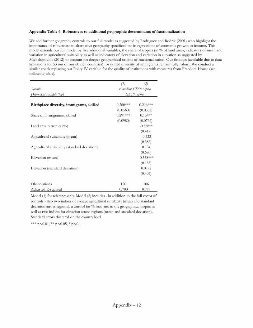
Appendix – 12

Appendix Table 6: Robustness to additional geographic determinants of fractionalization We add further geography controls to our full model as suggested by Rodriguez and Rodrik (2001) who highlight the importance of robustness to alternative geography specifications in regressions of economic growth or income. This model extends our full model by five additional variables, the share of tropics (in % of land area), indicators of mean and variation in agricultural suitability as well as indicators of elevation and variation in elevation as suggested by Michalopoulos (2012) to account for deeper geographical origins of fractionalization. Our findings (available due to data limitations for 53 out of our 60 rich countries) for skilled diversity of immigrants remain fully robust. We conduct a similar check replacing our Polity IV variable for the quality of institutions with measures from Freedom House (see following table).

(1) (2)

Sample

Dependent variable (log)

Birthplace diversity, immigrants, skilled 0.260*** 0.216***

(0.0560) (0.0582)

Share of immigration, skilled 0.291*** 0.154**

(0.0980) (0.0766)

Land area in tropics (%) -0.888**

(0.417)

Agricultural suitability (mean) -0.533

(0.386)

Agricultural suitability (standard deviation) 0.734

(0.680)

Elevation (mean) -0.558***

(0.185)

Elevation (standard deviation) 0.0772

(0.405)

Observations 120 106

Adjusted R-squared 0.700 0.779

*** p<0.01, ** p<0.05, * p<0.1

> median GDP/capita

GDP/capita

Model (1) for reference only. Model (2) includes - in addition to the full vector of

controls - also two indices of average agricultural suitability (mean and standard

deviation across regions), a control for % land area in the geographical tropics as

well as two indices for elevation across regions (mean and standard deviation).

Standard errors clustered on the country level.

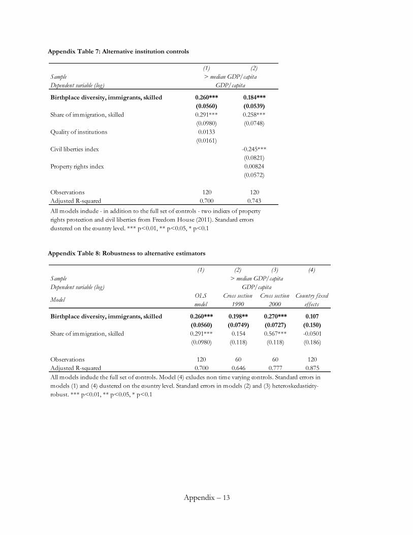
Appendix – 13

Appendix Table 7: Alternative institution controls

Appendix Table 8: Robustness to alternative estimators

(1) (2)

Sample

Dependent variable (log)

Birthplace diversity, immigrants, skilled 0.260*** 0.184***

(0.0560) (0.0539)

Share of immigration, skilled 0.291*** 0.258***

(0.0980) (0.0748)

Quality of institutions 0.0133

(0.0161)

Civil liberties index -0.245***

(0.0821)

Property rights index 0.00824

(0.0572)

Observations 120 120

Adjusted R-squared 0.700 0.743

> median GDP/capita

GDP/capita

All models include - in addition to the full set of controls - two indices of property

rights protection and civil liberties from Freedom House (2011). Standard errors

clustered on the country level. *** p<0.01, ** p<0.05, * p<0.1

(1) (2) (3) (4)

Sample

Dependent variable (log)

ModelOLS

model

Cross section

1990

Cross section

2000

Country f ixed

ef f ects

Birthplace diversity, immigrants, skilled 0.260*** 0.198** 0.270*** 0.107

(0.0560) (0.0749) (0.0727) (0.150)

Share of immigration, skilled 0.291*** 0.154 0.567*** -0.0501

(0.0980) (0.118) (0.118) (0.186)

Observations 120 60 60 120

Adjusted R-squared 0.700 0.646 0.777 0.875

All models include the full set of controls. Model (4) exludes non time varying controls. Standard errors in

models (1) and (4) clustered on the country level. Standard errors in models (2) and (3) heteroskedasticity-

robust. *** p<0.01, ** p<0.05, * p<0.1

> median GDP/capita

GDP/capita

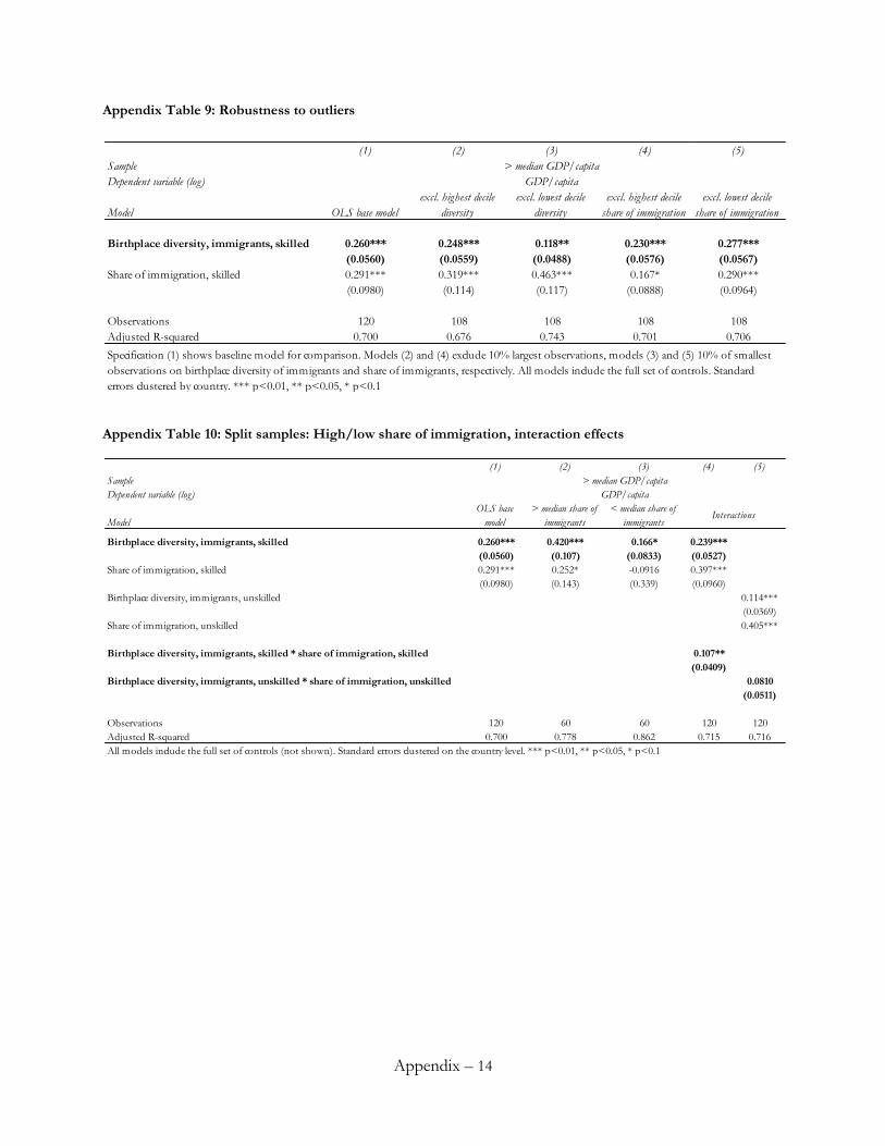
Appendix – 14

Appendix Table 9: Robustness to outliers

Appendix Table 10: Split samples: High/low share of immigration, interaction effects

(1) (2) (3) (4) (5)

Sample

Dependent variable (log)

Model OLS base model

excl. highest decile

diversity

excl. lowest decile

diversity

excl. highest decile

share of immigration

excl. lowest decile

share of immigration

Birthplace diversity, immigrants, skilled 0.260*** 0.248*** 0.118** 0.230*** 0.277***

(0.0560) (0.0559) (0.0488) (0.0576) (0.0567)

Share of immigration, skilled 0.291*** 0.319*** 0.463*** 0.167* 0.290***

(0.0980) (0.114) (0.117) (0.0888) (0.0964)

Observations 120 108 108 108 108

Adjusted R-squared 0.700 0.676 0.743 0.701 0.706

Specification (1) shows baseline model for comparison. Models (2) and (4) exclude 10% largest observations, models (3) and (5) 10% of smallest

observations on birthplace diversity of immigrants and share of immigrants, respectively. All models include the full set of controls. Standard

errors clustered by country. *** p<0.01, ** p<0.05, * p<0.1

> median GDP/capita

GDP/capita

(1) (2) (3) (4) (5)

Sample

Dependent variable (log)

Model

OLS base

model

> median share of

immigrants

< median share of

immigrants

Birthplace diversity, immigrants, skilled 0.260*** 0.420*** 0.166* 0.239***

(0.0560) (0.107) (0.0833) (0.0527)

Share of immigration, skilled 0.291*** 0.252* -0.0916 0.397***

(0.0980) (0.143) (0.339) (0.0960)

Birthplace diversity, immigrants, unskilled 0.114***

(0.0369)

Share of immigration, unskilled 0.405***

Birthplace diversity, immigrants, skilled * share of immigration, skilled 0.107**

(0.0409)

Birthplace diversity, immigrants, unskilled * share of immigration, unskilled 0.0810

(0.0511)

Observations 120 60 60 120 120

Adjusted R-squared 0.700 0.778 0.862 0.715 0.716

> median GDP/capita

GDP/capita

Interactions

All models include the full set of controls (not shown). Standard errors clustered on the country level. *** p<0.01, ** p<0.05, * p<0.1