biodiversity in two parts: environmental heterogeneity and ... · ii biodiversity in two parts:...
TRANSCRIPT

Biodiversity in two parts: environmental heterogeneity and the maintenance of diversity, and the prioritization
of diversity
by
Caroline Marie Tucker
A thesis submitted in conformity with the requirements for the degree of Doctor of Philosophy
Ecology and Evolutionary Biology University of Toronto
© Copyright by Caroline M. Tucker 2013

ii
Biodiversity in two parts: environmental heterogeneity and the maintenance of diversity, and the prioritization
of diversity Caroline Marie Tucker
Doctor of Philosophy
Ecology and Evolutionary Biology University of Toronto
2013
Abstract
Questions surrounding the causes and consequences of diversity lie at the centre of
community ecology. Understanding the mechanisms by which species diversity is
maintained motivates much experimental and theoretical work, but this work often
focuses on fluctuation-independent mechanisms. Variability in habitat suitability is
ubiquitous through space and time however, and provides another important path through
which species diversity can be maintained. As a result, considering environmental
variability has value for conservation and management. Finally, differences through
space and time in the mechanisms that promote and maintain diversity produce spatially
varying patterns of diversity. Spatial variation in different forms of diversity (species
(SR), phylogenetic (PD), and functional diversity (FD)) creates difficult decisions about
prioritization and reserve locations.
This thesis uses experimental, observational, and theoretical methods to explore the
causes and consequences of diversity. I show that variation in space and time has
important implications for species coexistence and diversity maintenance. In microbial
nectar communities, temperature variation through space and time alters the importance

iii
of priority effects on community assembly. Using models of warming temperatures in
annual plant communities I show that considering temporal partitioning of flowering (a
strategy to minimize competition) introduces constraints on phenological shifts: this has
implications for phenological monitoring programs. Finally, I show that variability in the
timing of fire events in Mediterranean shrublands contributes to coexistence between life
forms, suggesting that it should be considered for fire management. In the final two
chapters, I focus on conservation prioritization. Comparisons of species richness and
evolutionary diversity through space in the Cape Floristic Region of South Africa show
that existing reserves protect Proteaceae richness, but fail to capture evolutionary distinct
species. More generally, in the final chapter I suggest that SR and PD should be
congruent through space when species are of similar ages, regions are depauperate, or
ranges are discontinuous.

iv
Acknowledgments
Above all, many thanks to my supervisor Marc Cadotte, who was good Samaritan,
Cheerleader and Sage all along. Without his support this degree wouldn’t have had a
middle or an end. Thanks to my extended lab family for all the support and general good
times they have provided: Lanna Jin, Nick Mirotchnick, Kelly Carscadden, Stuart
Livingstone, and Carlos Arnillas.
In no particular order, thanks to all the faculty members who were incredibly generous
with their time and expertise including Peter Abrams, Ben Gilbert, T.J. Davies, Art Weis,
Marie-Josee Fortin and Tadashi Fukami. Equally valuable were the fellow grad students
who shared their knowledge with me, especially Josie Hughes, Stephen Walker, Dak de
Kerckhove, and Jordan Pleet. In addition, thanks to my Scarborough cohort (Maria
Modanu, Emily MacLeod, Devin Bloom, and Tiffany Schriever), who were sources of
constant peer support.
For their constant support, Anna, John, and Michael Tucker have played a special role in
my success, and will continue to do so in the future. My gratitude to Anna Tucker and
Patrick Tucker who introduced me to the world of plants and nature.
Finally, thank you to my committee members: Helene Wagner, Ben Gilbert, Don
Jackson for patiently letting me find my feet as a scientist.

v
Table of Contents
Acknowledgments.......................................................................................................................... iv
Table of Contents ............................................................................................................................ v
List of Figures ................................................................................................................................ ix
List of Appendices ........................................................................................................................ xii
Introduction: Understanding patterns of diversity .......................................................................... 1
References....................................................................................................................................... 9
Chapter 1 Environmental Variability Counteracts Priority Effects to Facilitate Species Coexistence: Evidence from Nectar Microbes......................................................................... 13
1 1................................................................................................................................................ 13
1.1 Abstract ............................................................................................................................. 13
1.2 Introduction....................................................................................................................... 13
1.3 Methods............................................................................................................................. 15
1.3.1 Study organisms.................................................................................................... 15
1.3.2 Experimental flowers ............................................................................................ 16
1.3.3 Experimental design.............................................................................................. 16
1.3.4 Dispersal between flowers .................................................................................... 17
1.3.5 Population density estimation ............................................................................... 18
1.3.6 Supplementary experiments.................................................................................. 18
1.4 Results............................................................................................................................... 19
1.5 Discussion ......................................................................................................................... 20
1.6 Acknowledgements........................................................................................................... 22
References..................................................................................................................................... 23
Figures........................................................................................................................................... 25
Appendices.................................................................................................................................... 29

vi
Chapter 2 Community-level interactions alter species responses to climate change.................... 33
2 2................................................................................................................................................ 33
2.1 Abstract ............................................................................................................................. 33
2.2 Introduction....................................................................................................................... 34
2.3 Model and Results............................................................................................................. 35
2.3.1 Model .................................................................................................................... 35
2.3.2 Simulations ........................................................................................................... 37
2.3.3 Results................................................................................................................... 39
2.4 Discussion ......................................................................................................................... 40
2.5 Acknowledgements........................................................................................................... 43
References..................................................................................................................................... 44
Figures........................................................................................................................................... 48
Appendices.................................................................................................................................... 53
Chapter 3 Fire variability, as well as frequency, can explain coexistence between seeder and resprouter life histories........................................................................................... 57
3 3................................................................................................................................................ 57
3.1 Abstract ............................................................................................................................. 57
3.1.1 Synthesis and applications. ................................................................................... 57
3.2 Introduction....................................................................................................................... 58
3.3 Materials and methods ...................................................................................................... 60
3.3.1 Lottery model........................................................................................................ 60
3.3.2 A disturbance-based storage effect ....................................................................... 63
3.3.3 Numerical simulations .......................................................................................... 64
3.3.4 Parameter value selection ..................................................................................... 65
3.3.5 Sensitivity of the model to parameter values........................................................ 66
3.4 Results............................................................................................................................... 67

vii
3.4.1 Coexistence with non-variable fire return: ........................................................... 67
3.4.2 Coexistence with variable fire return.................................................................... 67
3.4.3 Influence of parameter values on coexistence ...................................................... 68
3.5 Discussion ......................................................................................................................... 68
3.5.1 Management implications..................................................................................... 70
References..................................................................................................................................... 71
Figures........................................................................................................................................... 76
Appendices.................................................................................................................................... 82
Copyright Acknowledgements...................................................................................................... 84
Chapter 4 Incorporating geographical and evolutionary rarity into conservation prioritization............................................................................................................................. 85
4 4................................................................................................................................................ 85
4.1 Abstract ............................................................................................................................. 85
4.2 Introduction....................................................................................................................... 86
4.3 Methods............................................................................................................................. 88
4.3.1 Study Area ............................................................................................................ 88
4.3.2 Data sources .......................................................................................................... 88
4.3.3 Phylogeny ............................................................................................................. 89
4.3.4 Diversity................................................................................................................ 90
4.3.5 Biogeographically weighted evolutionary distinctiveness.................................... 91
4.3.6 Metrics with genera-level tree .............................................................................. 92
4.3.7 Reserve representation indices.............................................................................. 92
4.4 Results............................................................................................................................... 93
4.5 Discussion ......................................................................................................................... 94
References..................................................................................................................................... 98
Figures......................................................................................................................................... 101

viii
Appendices.................................................................................................................................. 104
Copyright Acknowledgements.................................................................................................... 110
Chapter 5 Unifying measures of biodiversity: understanding when richness and phylogenetic diversity should be congruent........................................................................... 111
5 5.............................................................................................................................................. 111
5.1 Abstract ........................................................................................................................... 111
5.2 Introduction..................................................................................................................... 112
5.3 Unifying biodiversity measures ...................................................................................... 116
5.3.1 Conceptual underpinning of biodiversity measures............................................ 117
5.3.2 Exploring the correlation between metrics ......................................................... 118
5.3.3 Tree structure ...................................................................................................... 118
5.3.4 Spatial structure and abundance distribution ...................................................... 120
5.3.5 Species pool size ................................................................................................. 120
5.4 Conclusions: Securing the place for evolution and rarity in conserving biodiversity ..................................................................................................................... 121
References................................................................................................................................... 124
Figures......................................................................................................................................... 128
Appendices.................................................................................................................................. 133
Copyright Acknowledgements.................................................................................................... 135
Conclusions: Accounting for diversity in a changing world ...................................................... 136
References................................................................................................................................... 141

ix
List of Figures
Figure 1-1. Temporal changes in mean species abundances (± standard errors, n=4
metacommunity replicates), averaged over the paired flowers for each metacommunity,
when species were introduced in different timings in a constant or variable environment. ......... 25
Figure 1-2. Characterization of the common species Metschnikowia reukaufii and
Gluconobacter sp. ......................................................................................................................... 26
Figure 1-3. Graphical representation of one hypothesis for how environmental variability
promotes species coexistence when species arrive sequentially, but not simultaneously in
the experimental system of nectar microbes. ................................................................................ 27
Figure 2-1. Rate of allocation to reproduction (i.e 1/Di) for species 1-4. Species’ optimal
temperatures are 19, 20, 21, 22°C, respectively. .......................................................................... 48
Figure 2-2. Randomly simulated temperatures for 1000 years, shaded area represents the
range of the possible values, the dashed line represents the mean temperature under a)
ambient conditions and b) warming conditions (+2°C)................................................................ 49
Figure 2-3. Boxplots of Julian day of first flower over 1000 simulated years for four
species. Blue boxes represent ambient temperature conditions (either light blue for no
competition or dark blue for competition) and pink boxes represent warming (+2°C)
conditions (light pink, no competition or dark pink for competition). ......................................... 50
Figure 2-4. Change in the average Julian day of first flower in response to changing
species developmental overlap for species 1-4. ............................................................................ 51
Figure 2-5. Proportional distribution of flowering times Figure 3, for species 1-4, across
all combinations of warming and competition treatments. ........................................................... 52
Figure 3-1. Conceptual model showing the number of seeds available for recruitment (βi,
Equation 2) as a function of the length of the inter-fire interval (f) for a generic seeder
x
(red) and resprouter (black) species. c=8000 and a=50. See Materials and methods for
further details on parameterization. .............................................................................................. 76
Figure 3-2. A. Mean inter-fire intervals for which coexistence or exclusion between
seeder and resprouter species is expected, when the length of the inter-fire interval is
invariant. c=8000 and a=50. 5 regions of inter-fire intervals are highlighted; grey regions
indicate where long-term persistence is predicted. ....................................................................... 77
Figure 3-3. The probability of coexistence between the seeder and resprouter species, as a
function of both the length of the inter-fire interval and variation in the fire return
interval. ......................................................................................................................................... 79
Figure 3-4. The probability of coexistence between seeders and resprouters when there is
no storage for the resprouter species (i.e. δ = 1), as a function of the length of the inter-
fire interval and variation in the length of the inter-fire interval. ................................................. 80
Figure 3-5. The interaction between the number of seeds available for recruitment and
resprouter mortality (δ), and their effect on the minimum amount of variation in the inter-
fire interval necessary for coexistence. ......................................................................................... 81
Figure 4-1. Pearson correlation coefficients showing the strength of the relationships
among species richness, phylogenetic diversity (PD), and biogeographically weighted
evolutionary distinctiveness (BEDT) metrics for Proteaceae in the Cape Floristic Region,
South Africa (none, species lacking sequence data not included; low, species lacking
sequence data included at low evolutionary diversity position; high, species lacking
sequence data included at high evolutionary diversity position; genera, resolved only to
the level of genus). ...................................................................................................................... 101
Figure 4-2. Proteaceae diversity of 311 species in the Cape Floristic Region on the
southern tip of Africa, diversity is measured using (a) species richness, (b) phylogenetic
diversity, and (c) biogeographically weighted ecological distinctiveness, where (b) and
(c) were calculated using the low tree, where species lacking sequence data were included
at low evolutionary diversity position......................................................................................... 102
xi
Figure 4-3. (a) The relation between biogeographically weighted evolutionary
distinctiveness (BEDT) and range size (calculated as the square-root transformed number
of cells occupied by the species) and (b) distribution of range size for the ‘none’
phylogenetic tree, where Proteaceae species lacking species data are not included. ................. 103
Figure 5-1. Comparison of the four types of biogeographical diversity metrics that use
different types of information. .................................................................................................... 128
Figure 5-2. Examples of the range of tree topology simulated................................................... 129
Figure 5-3. Spearman’s correlation (r) between species richness (SR) and phylogenetic
diversity (PD) as a function of tree topology.............................................................................. 130
Figure 5-4. A) Spearman’s correlation (r) between biogeographically-weighted species
richness (BSR) and biogeographically-weighted evolutionary distinctivness (BED), as a
function of tree topology and species range sizes. B) Spearman’s correlation (r) between
phylogenetic diversity (PD) and biogeographically-weighted evolutionary distinctivness
(BED), as a function of tree topology and species range sizes. .................................................. 131
Figure 5-5. The expected correlation between species richness (SR) and phylogenetic
diversity (PD) as a function of tree topology, species pool size and spatial autocorrelation. .... 132

xii
List of Appendices
Appendix 1-1. Temperature variability......................................................................................... 29
Appendix 1-2. Temporal changes in mean species abundances when species were
introduced in different arrival timings with either spatial or temporal environmental
(temperature) variability. Symbols are as in Figure 1-1. .............................................................. 31
Appendix 1-3. Consumer-resource model used to produce zero-net growth isoclines
(ZNGIs), modelling competition for resources (amino acids) between a bacteria species
(representing Gluconobacter) producing an inhibitor (pH) and a yeast species
(representing Metschnikowia). ...................................................................................................... 32
Appendix 2-1. Parameter values used for model simulations....................................................... 53
Appendix 2-2. R code for model and simulations of warming in annual plant
communities. ................................................................................................................................. 53
Appendix 3-1. R code for the disturbance-based storage model .................................................. 82
Appendix 4-1. Phylogenetic tree of the CFR Proteaceae, constructed using sequences
from Genbank. ............................................................................................................................ 104
Appendix 4-2. Graphical representation of how a species, D, lacking sequence data,
would be positioned on the phylogenetic tree, based on branch lengths, relative to its
congeners A, B, and C with sequence data. ................................................................................ 108
Appendix 4-3. Reserve representation index for 311 species of Proteaceae in the Cape
Floristic Region, a biodiversity hotspot on the southern tip of Africa. The maps illustrate
prioritization of a, species diversity or b, phylogenetic diversity, outside of reserve sites:
Phylogenetic or species diversity is scaled by degree of representation within the existing
reserve network species to highlight remaining areas with less represented phylogenetic
or species diversity (see Methods). ............................................................................................. 109
Appendix 5-1. Simulation methods. ........................................................................................... 133

xiii
Appendix 5-2. A) Effect of spatial autocorrelation in species occupancy on the correlation
between the four biodiversity metrics; B) Effect of regional species pool size on the
strength of the correlation between the four biodiversity metrics. ............................................. 134

1
Introduction: Understanding patterns of diversity
Species diversity has long been the central focus of community ecology. Questions relating to
how many species coexist, their particular identities, and their distribution and abundances
consumed the earliest ecologists, and were answered with the belief that nature was predictable
and ordered and that discoverable mechanisms explained diversity (McIntosh 1985). Modern
ecologists have expanded their definition of diversity to incorporate all forms of biological
diversity, “the variability among living organisms from all sources including, inter alia,
terrestrial, marine and other aquatic ecosystems and the ecological complexes of which they are
part; this includes diversity within species, between species and of ecosystems” (United Nations
1992). They also place more emphasis on the role of chance and stochastic processes (Drake et
al. 1999; Hubbell 2001). However, a central goal remains explaining the patterns and processes
behind global biological diversity (e.g. Andrewartha & Birch 1954; Hutchinson 1961;
MacArthur & Wilson 1967; Whittaker 1967; Brown 1984; Chesson 2000; Hubbell 2001).
There are two approaches to understanding global patterns of biodiversity – one can focus on
large-scale patterns of diversity which reflect how diversity is produced over evolutionary time
scales via speciation and extinction events, or alternately one can focus on how local interactions
in ecological time allow the coexistence of species and therefore the maintenance of diversity.
Together these approaches contribute to a holistic understanding of diversity, but represent
different spatial and temporal lenses. Research on the production of diversity is particularly
focused on explanations for patterns of diversity over large spatial scales (e.g. macroecology
(Brown 1999; Gaston & Blackburn 2000)), its relationship with latitudinal or elevational
gradients (Hillebrand 2004; Mittelbach et al. 2007), and the evolutionary and ecological
processes influencing speciation and extinction (Losos 2011; Wiens 2012). Patterns of diversity
over biogeographical spatial scales tend to be the focus of conservation activities as well
(Mittermeier et al. 1998; Myers et al. 2000). In contrast, interest in the maintenance of diversity
has long been inspired by the paradox of coexistence – how can ecologically similar species and
limited resources somehow manage to stably co-occur through time (Hutchinson 1961)? Many
mechanisms have been suggested to play a role in mediating competitive interactions between
species (e.g. Grubb 1977; Chesson 2000; Grime 2001; Wilson 2011), and this remains an area of
2
continued interest. These contrasting approaches to studying biodiversity provide complementary
information about the causes, maintenance and consequences of biodiversity. My thesis
considers both: in the first three chapters, I focus on mechanisms of biodiversity maintenance
over small spatial scales, in particular, for communities or guilds of species. The second half
considers biogeographical-scale patterns of diversity and focuses on how differences in the
importance of processes originating species and evolutionary diversity result in spatially
incongruent patterns of these forms of diversity. This is important both for understanding how
diversity is produced at large spatial scales and what the implications of this are for conservation
and management.
Part 1: The maintenance of diversity in local communities.
Diversity maintenance can be defined as coexistence in the same spatial region by ecologically
similar species (Chesson 2000). Gause’s “law” of competitive exclusion states that two species
competing for the same resource cannot coexist (Gause 1934). Because multiple species persist
in ecological communities, ecologists have had cause to explore numerous mechanisms that
might explain the maintenance of this diversity. While a comprehensive framework
incorporating the many suggested mechanisms of coexistence is lacking, Chesson (2000)
suggested one possible unifying set of mechanisms: equalizing and stabilizing forces. Under this
framework, species stably coexist because niche differences (stabilizing forces) are large enough
for intraspecific competition to exceed interspecific competition. The size of niche differences
necessary for coexistence depends on the fitness inequality (equalizing forces) between the
competing species. Species with similar fitnesses should require smaller stabilizing forces to
coexist. Most mechanisms of coexistence can be reframed in terms of Chesson’s (2000)
framework, although this has not been done in a comprehensive manner. One consideration when
explaining mechanisms of coexistence is whether variability in environmental conditions plays a
role. However, although variability has received attention as a possible driver of species
coexistence (Hutchinson 1961; Wiens 1977; Chesson & Warner 1981; Warner & Chesson 1985),
for many ecosystems it has received less attention than fluctuation-independent mechanisms.
Given environmental variation is undeniably ubiquitous in natural systems, it should be a fruitful
area of focus.
3
Role for environmental heterogeneity: Environmental heterogeneity–here defined as variability
in patch suitability–occurs through time or space, and can facilitate coexistence (Wilson 2011).
Heterogeneity thus produces differences in a species’ success (e.g. recruitment) through time
and/or space. Heterogeneity arising from abiotic and biotic sources is ubiquitous throughout
many ecosystems at many spatial and temporal scales (e.g. Moore et al. 1993; Palmer & Poff
1997). Spatial heterogeneity, for example, can exist between microclimates in a habitat, between
habitats, and between ecosystems (Pickett & Cadenasso 1995). Spatial heterogeneity may be
driven by abiotic patterns (e.g. elevational or latitudinal trends in temperature (Gaston 2000)),
biotic patterns (e.g. limitations on dispersal (Levine & Murrell 2003) or neighbour identity
(Tilman 1994)). Temporal heterogeneity is similarly ubiquitous in natural systems and occurs on
a wide range of temporal scales (Ruel & Ayres 1999) and with differing patterns of
autocorrelation (Vasseur & Yodzis 2004). Most organisms experience some spatial and temporal
heterogeneity during their lifetimes, and as a result there is an increasing awareness of the need
to account for these factors (Ruel & Ayres 1999; Hewitt et al. 2007).
Heterogeneity encourages coexistence at the multi-patch or –time scale by providing a way for
species to partition their performance between spatial patches or times. Provided that species’
ecologies allow for movement between patches or survival of different temporal conditions,
coexistence of two or more species competing for limiting resources is possible (e.g. Slatkin
1974; Hanski 1983; Warner & Chesson 1985; Chesson 2000, 2003). Spatial and/or temporal
variation in habitat suitability has the effect of producing spatial and/or temporal variation in
recruitment. Temporal variability in recruitment results in lower growth rates than those
experienced under optimal conditions. In general variation contributes to coexistence either by
enhancing temporal/spatial partitioning or through non-linearity in competition (Chesson 2000).
Non-linearity of competition: Species often have non-linear responses to environmental
variables. For example, functional responses tend to be non-linear functions of limiting
resources. Jensen’s inequality states that for nonlinear functions, the average of the function (
€
f (x) ) is not equal to the function of the average (
€
f (x )). In practice this means that because
variation results in averaged recruitment rates across space and/or time, species with decelerating
functional responses tend to have decreased average recruitment when variation is present, while
accelerating functions result in species with higher average recruitment when variation is present.

4
The interaction between variability in the system and the shape of a species’ functional response
can therefore reduce or increase the competitive success of that species in relation to other
species (Ruel & Ayres 1999). Because non-linear averaging can reduce fitness differences
between individuals, it can be considered an equalizing force (Chesson 2000).
Spatial and temporal partitioning (i.e. the storage effect): Species can also partition or specialize
on subsets of the spatial and temporal conditions they experience. Spatial and temporal
partitioning of resources or habitat are fairly analogous mechanisms for coexistence: 1) species
need to exhibit differential responses to the environment; 2) covariance between competition and
the environment; and, 3) a mechanism for buffered population growth (Chesson 2000).
“The first and third components are largely determined by how different
environmental conditions affect the utilization rates of the limiting resource by
two (or more) competing species. When two species have different relationships
between utilization rate of a resource and one or more varying environmental
factors, a rare species can achieve a high per capita growth rate under conditions
that allow it to have a much greater utilization rate and/or competitive ability
than its competitor(s)” (Abrams et al. 2012).
In the spatial case, buffering mechanisms could simply be dispersal between patches with
different growth rates (Amarasekare 2003); in the temporal case, they might include seed banks
(Angert et al. 2009) or long-lived dormant stages (Caceres 1997). Storage effect type
mechanisms allow species to decrease the strength of their interactions by becoming increasingly
specialized on a subset of the possible conditions, thereby acting as a stabilizing effect (Chesson
2000).
Environmental conditions are inherently variable and there are numerous ways that species can
take advantage of this heterogeneity to facilitate competitive coexistence. Environmental
heterogeneity in its many forms is suggested to play a role in coexistence between plants in
general (Ricklefs 1977), desert annuals (Angert et al. 2007; Huxman et al. 2008; Kimball et al.
2011), Mediterranean shrubs (Tucker & Cadotte, In press), invertebrates (Ranta &
Vepsalaininen 1981), protists (Gause 1934; Caceres 1997), as well as many others. As a result, it
is not surprising that diversity in many systems is dependent on the continued occurrence of

5
environmental variability. For this reason, understanding the mechanisms by which
environmental variability contributes to biodiversity is also valuable for management and
conservation activities.
Part 2: Using large-scale patterns of diversity to inform prioritization
Ecological dynamics are changing globally for a number of reasons. Climate is changing,
including increasing mean temperatures and decreasing precipitation and snowfall (IPCC 2007).
The amount of variability in climate conditions is also changing – the extremes of temperature
and precipitation values are increasing along with overall variation (Karl et al. 1995; Folland et
al. 2002). Changes in disturbance regimes accompany these climatic changes, for example
modifying the frequency, intensity, and extent of fire events (Gillet et al. 2004). Changes in
climate and disturbance regimes, combined with habitat loss and fragmentation have contributed
to a century of species extinctions (Groombridge 1992; Heywood & Watson 1995).
In response to the potential for extinctions, conservation activities include selecting vulnerable or
valuable regions for protection (Myers et al. 2000; Mittermeier & Cemex 2004), managing land
for values such as diversity maintenance, and restoring damaged sites (Hunter Jr 1990; White &
Walker 1997; Grumbine 2002). These activities tend to focus on diversity with a regional lens,
because changes in climate and human activities act at a large scale. In addition, there is a
recognition that “biodiversity” is similarly broad, and encompasses all forms of organismal
variety, from genetic variation to the differences in the richness of higher taxa, and diversity in
ecosystem structure and function in conservation activities (Wilson & Peter 1988). In any
geographical region of interest, spatial patterns of different forms of diversity vary. This makes it
difficult to capture all types of diversity in a single protected area, for example. Combined with
limited funds, this creates the need to prioritize regions and/or types of taxa, a problem described
as the agony of choice (Vane-Wright 1991). By focusing on multiple types of diversity in regions
of interest, researchers can gain important information about the processes at play and informs
prioritization of areas for reserve locations. As a result, the focus of prioritization is becoming
increasingly multidimensional with regards to optimal reserve selection and protection of
diversity (Faith 1992; Rodrigues et al. 2005; Forest et al. 2007; Huang et al. 2011; Tucker et al.
2012a).

6
Chapter overviews
In this thesis, I will consider these two broad areas of ecological research, examining first the
mechanisms by which spatial and temporal heterogeneity promotes diversity maintenance in
communities and secondly how spatially variable patterns of biodiversity in biogeographical
regions inform conservation and management activities.
Part 1: The maintenance of diversity in local communities
1) Environmental Variability Counteracts Priority Effects to Facilitate Species Coexistence:
Evidence from Nectar Microbes.
In the first chapter, I explore whether variability in temperature through space and/or time affects
the assembly of floral microbial communities, and further whether it alters the contribution of
priority effects to community assembly. Priority effects have received the majority of attention as
a determinant of species diversity and identity in nectar microbial communities, but natural
communities of nectar yeast and bacteria also experience temperature variation over a wide
variety of scales. In this chapter, I examine the possibility that environmental heterogeneity may
alter the outcome of other mechanisms of diversity maintenance using experimental
manipulations and mathematical models.
2) Community-level Interactions Alter Species’ Responses to Climate Change.
The second chapter focuses on a different scale of temporal variability, the importance of intra-
seasonal partitioning by competing annual plants and the effect of increasing temperatures on
this. To minimize competitive interactions during their growing season, annual plants often
minimize temporal co-occurrence by differentially specializing on particular subsets of
temperature, precipitation and photoperiod conditions during the season. In annual plant
communities structured in this way, climate change may affect the temperature-sensitive timing
of reproduction, and the degree of competition between species in a community. This may have
important implications for studies of shifts in plant phenology in response to global climate
change, because it suggests a constraint–biotic interactions—rarely considered when using
phenological measures as indicators of changing climate.

7
3) Fire Variability, as well as Frequency, can Explain Coexistence Between Seeder and
Resprouter Life Histories.
In the third chapter, I use theory and modelling to explore whether temporal variation in fire
occurrences can help to promote coexistence between two life histories of Mediterranean shrubs.
Evidence that such variability in fire events mediates a storage effect would have implications
for fire management plans and the question of whether maintaining natural variation in planned
burns is likely to be important for diversity maintenance.
Part 2: Using large-scale patterns of diversity to inform prioritization
4) Incorporating Geographical and Evolutionary Rarity into Conservation Prioritization.
A variety of mechanisms, including temporal and spatial variability in disturbance and climate,
have led to high levels of angiosperm diversity and endemism in Mediterranean ecosystems. As a
result, all Mediterranean ecosystems are declared biodiversity hotspots (Myers et al. 2000). For
example, in the Cape Floristic Region of South Africa, there are a number of international,
national, and provincially established protected areas that capture a high proportion of the
Proteaceae species in the region. However, other forms of diversity were not considered when
the initial reserves were established. In the fourth chapter, I examine how well existing reserve
networks capture phylogenetic diversity (PD) and biogeographically-weighted evolutionary
diversity (BED), as well as Proteaceae richness, and consider the implications for conservation in
the Cape Floristic Region.
5) Unifying measures of biodiversity: understanding when richness and phylogenetic diversity
should be congruent
Not surprisingly, spatial patterns of species richness often differ from spatial patterns of
evolutionary diversity or functional diversity, because ecological and evolutionary processes do
not occur evenly through space, and since ecological processes contribute differentially to
different types of diversity. In this chapter, I develop a predictive framework to help understand
the conditions under which we expect species richness and evolutionary history in communities
to be differentially or similarly distributed through space, using information about a region’s
evolutionary history and spatial structure.

8
Conclusions
Across these five chapters, common themes include the understanding the mechanisms behind
diversity maintenance in local communities, with a particular focus on environmental
heterogeneity, and the implications of this information for management and conservation
activities. I hope to show that environmental variability is important for ecological processes
such as coexistence because it is ubiquitous, it alters species demographic responses, and human
actions and changing climate are altering drivers of variability. In addition I look at large-scale
patterns of diversity, particularly contrasting patterns of species richness and evolutionary
history, to inform diversity prioritization and conservation. This multi-scale, multi-method
approach allows me to more completely explore these important questions in ecology.

9
References
Abrams P.A., Tucker C.M. & Gilbert B. (2012). The evolution of the storage effect. Evolution, In press.
Amarasekare P. (2003). Competitive coexistence in spatially structured environments: a synthesis. Ecology Letters, 6, 1109-1122.
Andrewartha H.G. & Birch L.C. (1954). The distribution and abundance of animals. University of Chicago Press, Chicago.
Angert A.L., Huxman T.E., Barron-Gafford G.A., Gerst K.L. & Venable D.L. (2007). Linking growth strategies to long-term population dynamics in a guild of desert annuals. Journal of Ecology, 95, 321-331.
Angert A.L., Huxman T.E., Chesson P. & Venable D.L. (2009). Funtional tradeoffs determine species coexistence via the storage effect. Proceedings of the National Academy of Sciences of the United States of America, 106, 11641-11645.
Brown J.H. (1984). On the relationship between distribution and abundance. The American Naturalist, 124, 255-279.
Brown J.H. (1999). Macroecology: Progress and prospect. Oikos, 87, 3-14.
Caceres C.E. (1997). Temporal variation, dormancy, and coexistence: a field test of the storage effect. Proceedings of the National Academy of Sciences of the United States of America, 94, 9171-9175.
Chesson P. (2000). Mechanisms of maintenance of species diversity. Annual Review of Ecology and Systematics, 31, 343-366.
Chesson P. (2003). Quantifying and testing coexistence mechanisms arising from recruitment fluctuations. Theoretical Population Biology, 4, 345-357.
Chesson P. & Warner R.R. (1981). Environmental variability promotes coexistence in lottery competitive systems. American Naturalist, 117, 923-943.
Drake J.A., Zimmerman C.R., Purucker T. & Rojo C. (1999). On the nature of the assembly trajectory. In: Ecological Assembly Rules: Perspectives, advances, retreats (eds. Keddy PA & Weiher E). Cambridge University Press Cambridge, UK.
Faith D.P. (1992). Conservation evaluation and phylogenetic diversity. Biological Conservation, 61, 1-10.
Folland C.K., Karl T.R. & Salinger M.J. (2002). Observed climate variability and change. Weather, 57, 269-278.
Forest F., Grenyer R., Rouget M., Davies T.J., Cowling R.M., Faith D.P., Balmford A., Manning J., Proches S., van der Bank M., Reeves G., Hedderson T.A.J. & Savolainen V. (2007). Preserving the evolutionary potential of floras in biodiversity hotspots. Nature, 445, 757-760.
Gaston K.J. (2000). Global patterns in biodiversity. Nature, 405, 220-227.
10
Gaston K.J. & Blackburn T.M. (2000). Pattern and proccess in Macroecology. Blackwell Science.
Gause G.F. (1934). The struggle for existence. Williams & Wilkins, Baltimore.
Gillet N., Weaver A., Zwiers F. & Flannigan M. (2004). Detecting the effects of climate change on Canadian forest fires. Geophysical Research Letters, 31.
Grime J.P. (2001). Plant strategies, vegetation processes, and ecosystem properties. 2nd edn. John Wiley & Sons Ltd, West Sussex.
Groombridge B. (1992). Global Biodiversity: status of the earth living resources. In: London.
Grubb P.J. (1977). The maintenance of species-richness in plant communities: the importance of the regeneration niche. Biological Reviews, 52, 107-145.
Grumbine R.E. (2002). What is ecosystem management? Conservation Biology, 8, 27-38.
Hanski I. (1983). Coexistence of competitors in a patchy environment. Ecology, 64, 493-500.
Hewitt J.E., Thrush S.F., Dayton P.K. & Bonsdorf E. (2007). The effect of spatial and temporal heterogeneity on the design and analysis of empirical studies of scale-dependent systems. The American Naturalist, 169, 398-408.
Heywood V.H. & Watson R.T. (1995). Global biodiversity assessment. Cambridge University Press.
Hillebrand H. (2004). On the generality of the latitudinal diversity gradient. The American Naturalist, 163, 192-211.
Huang J., Chen B., Liu C., Lai J., Zhang J. & Ma K. (2011). Identifying hotspots of endemic woody seed plant diversity in China. Diversity and Distributions, 7, 673-688.
Hubbell S.P. (2001). The Unified Neutral Theory of Biodiversity and Biogeography. Princeton University Press.
Hunter Jr M.L. (1990). Wildlife, Forests, and Forestry. Principles of Managing Forests for Biological Diversity. Prentice Hall.
Hutchinson G.E. (1961). The Paradox of the plankton. The American Naturalist, 95, 137-145.
Huxman T.E., Barron-Gafford G.A., Gerst K.L., Angert A.L., Tyler A.P. & Venable D.L. (2008). Photosynthetic resource-use efficiency and demographic variability in desert winter annual plants. Ecology, 89, 1554-63.
IPCC (2007). Contribution of Working Groups I, II, and III to the fourth assessment report of thye Intergovernmental Panel on Climate Change. In: IPCC (eds. Pachauri RK & Reisinger A) Geneva, Switzerland.
Karl T.R., Knight R.W. & Plummer N. (1995). Trends in high-frequency variability in the twentieth century. Nature, 377, 217-220.
Kimball S., Gremer J.R., Angert A.L., Huxman T.E. & Venable D.L. (2011). Fitness and physiology in a variabile environment. Oecologia.
Levine J.M. & Murrell D.J. (2003). The community-level consequences of seed dispersal patterns. Annual Review of Ecology, Evolution, and Systematics, 34, 549-574.
11
Losos J.B. (2011). Convergence, adaptation, and constraint. Evolution, 65, 1827-1840.
MacArthur R.H. & Wilson E.O. (1967). The Theory of Island Biogeography. Princeton University Press, Princeton.
McIntosh R.P. (1985). The Background of Ecology: Concept and Theory. Cambridge University Press, Cambridge, U.K.
Mittelbach G.G., Schemske D.W., Cornell H.V., Allen A.P., Brown J.M., Bush M.B., Harrison S., Hurlbert A.H., Knowlton N., Lessios H.A., McCain C.M., McCune A.R., McDade L.A., McPeek M.A., Near T.J., Price T.D., Ricklefs R.E., Roy K., Sax D.F., Schluter D., Sobel J.M. & Turelli M. (2007). Evolution and the latitudinal diversity gradient: speciation, extinction and biogeography. Ecology Letters, 10, 315-331.
Mittermeier R.A. & Cemex S.A. (2004). Hotspots Revisited. Cemex, Mexico City, Mx.
Mittermeier R.A., Myers N., Thorsen J.B., da Fonseca G.A.B. & Olivier S. (1998). Biodiversity hotspots and major tropical wilderness areas: approaches to setting conservation priorities. Conservation Biology, 12, 516-520.
Moore I.D., Norton T. & Williams J.E. (1993). Modelling environmental heterogeneity in forested landscapes. Journal of Hydrology, 150, 717-747.
Myers N., Mittermeier R.A., Mittermeier C.G., da Fonseca G.A.B. & Kent J. (2000). Biodiversity hotspots for conservation priorities. Nature, 403, 853-858.
United Nations. (1992). Convention on Biological Diversity. In.
Palmer M.A. & Poff N.L. (1997). The Influence of Environmental Heterogeneity on Patterns and Processes in Streams. Journal of the North American Benthological Society, 16, 169-173.
Pickett S.T.A. & Cadenasso M.L. (1995). Landscape ecology: spatial heterogeneity in ecological systems. Science, 269, 331-334.
Ranta E. & Vepsalaininen K. (1981). Why are there so many species? Spatio-temporal heterogeneity and northern bumblebee communities. Oikos, 28-34.
Ricklefs R.E. (1977). Environmental heterogeneity and plant species diversity: a hypothesis. The American Naturalist, 111, 376-381.
Rodrigues A.S.L., Brooks T.M. & Gaston K.J. (2005). Integrating phylogenetic diversity in the selection of priority areas for conservation: does it make a difference? In: Phylogeny and Conservation (eds. Purvis A, Gittleman JL & Brooks TM). Cambridge University Press Cambridge, UK, pp. 101-199.
Ruel J.J. & Ayres M.P. (1999). Jensen's inequality predicts effects of environmental variation. Trends in Ecology & Evolution, 14, 361-366.
Slatkin M. (1974). Competition and regional coexistence Ecology, 55, 128-134.
Tilman D. (1994). Competition and biodiversity in spatially structured habitats. Ecology, 75, 2-16.
Tucker C.M., Cadotte M.W., Davies T.J. & Rebelo A.G. (2012). The distribution of biodiversity: linking richness to geographical and evolutionary rarity in a biodiversity hotspot Conservation Biology, In press.
12
Vane-Wright (1991). What to protect - systematics and the agony of choice. Biological Conservation, 55, 235-254.
Vasseur D.A. & Yodzis P. (2004). The color of environmental noise. Ecology, 85, 1146-1152.
Warner R.R. & Chesson P. (1985). Coexistence mediated by recruitment fluctuations: a field guide to the storage effect. The American Naturalist, 125, 769-787.
White P.S. & Walker J.L. (1997). Approximating nature's variation: selecting and using reference information in restoration ecology. Restoration Ecology, 5, 338-349.
Whittaker R.H. (1967). Gradient analysis of vegetation. Biological Reviews, 49, 207-264.
Wiens J.A. (1977). On Competition and Variable Environments: Populations may experience "ecological crunches" in variable climates, nullifying the assumptions of competition theory and limiting the usefulness of short-term studies of population patterns. American Scientist, 65, 590-597.
Wiens J.J. (2012). Phylogeny, ecology, and the origins of climate-richness relationships. Ecology, 93, S167-S181.
Wilson E.O. & Peter F.M. (1988). Biodiversity. National Academy Press, Washington.
Wilson J.B. (2011). The twelve theories of coexistence in plant communities: the doubtful, the important and the unexplored. Journal of Vegetation Science, 22, 184-195.

13
Chapter 1 Environmental Variability Counteracts Priority Effects to Facilitate
Species Coexistence: Evidence from Nectar Microbes
1 1
1.1 Abstract
The order of species arrival during community assembly can affect species coexistence, but the
strength of these effects, known as priority effects, is variable among species and across
ecosystems, and causes of this variation remain unclear. Here we show that environmental
variability can be one such cause. In experiments with nectar-inhabiting microorganisms that
disperse between flowers via pollinators, we manipulated spatial and temporal variability of
temperature and examined consequences for priority effects. If species arrived sequentially,
multiple species coexisted when temperature was variable, but not when it was constant.
Temperature variability prevented extinction of late-arriving species that would have been
excluded due to priority effects if temperature had been constant. In contrast, if species arrived
simultaneously, species coexisted under both variable and constant temperature. These results
suggest that understanding consequences of priority effects for species coexistence requires
consideration of how environmental variability alters the strength of priority effects.
1.2 Introduction
It is now widely recognized that variation in the order of species arrival among sites can drive
local communities to divergent successional trajectories, thereby affecting the coexistence of
species—the phenomenon known as priority effects (Sutherland 1974, 1990; Drake 1991; Chase
2003). However, studies of community assembly have yielded variable results as to the
importance of priority effects (Chase 2003) and identifying the causes of this variation remains
elusive. Although many potential causes have been considered (e.g. Chase 2003; Knowlton
2004; Fukami 2010), one likely cause, environmental variability, has rarely been investigated
despite the considerable interest it has long received as a factor affecting species coexistence
(e.g. Hutchinson 1961; Grubb 1977; Chesson & Warner 1981; Chesson 1985).

14
In theory, environmental variability may affect the strength of priority effects by changing
species growth rates (Loeuille & Leibold 2008). Priority effects are expected to be strong when
early-arriving species have high growth rates because they are then likely to pre-empt resources
or modify habitats rapidly enough to influence the performance of late-arriving species
(deFreitas & Frederickson 1978; Tilman 1980; Facelli & Facelli 1993). If environmental
variability makes growth rates temporally variable, it can result in overall reduction of growth
rates and therefore priority effects. This reduction occurs because the growth rate of a species
averaged over time is represented as the geometric, rather than arithmetic, mean, which is lower
than growth rates under constant environmental conditions (i.e. Jensen’s inequality)(Chesson
1985, 2000). In some circumstances, however, the amount of reduction in growth rates due to
environmental variability may differ among species when growth rates of some species are more
sensitive to environmental conditions than those of other species. In this case, whether
environmental variability weakens or strengthens priority effects may depend on the specific
relative response curves of different species to environmental conditions. For example, a tolerant
species would show a lesser decline in growth rate compared to a highly specialized or sensitive
species. Despite their potential to provide general explanations for when priority effects should
be strong, these theoretical ideas remain largely untested.
The purpose of this paper is to experimentally test the basic hypothesis that environmental
variability alters the influence of priority effects on community assembly. To this end, we
conducted a series of laboratory experiments using a simple model system, namely the
communities of yeast and bacterial species that inhabit the floral nectar of a hummingbird-
pollinated shrub in California (Belisle et al. 2012). Microbial systems provide many advantages
in testing general hypotheses regarding community assembly (reviewed in Drake et al. 1996;
Jessup et al. 2004; Cadotte et al. 2005) including short generation times and small habitat sizes
of microbial species, which allow community dynamics to be observed for many generations of
the species involved under rigorous experimental control over environmental conditions and
species arrival history.

15
Rapidly accumulating knowledge on the natural history of nectar-inhabiting microorganisms
(e.g. Herrera et al. 2008; Adam et al. 2011; Belisle et al. 2012; Fridman et al. 2012; Jacquemyn
et al. 2013) enables one to design naturally relevant experiments with these species. There is
evidence for strongly negative priority effects among some of these nectar-inhabiting species
(Peay et al. 2011), and ambient temperature is highly variable on a daily basis over both space
and time where the plants occur (Belisle et al. 2012). In the nectar microbial system, differences
in resource usage (amino acid and sugars) affect species interactions (Peay et al. 2011; Vannette
et al. 2013) and changes in nectar pH by acetic acid bacteria act as a barrier to community
invasion by yeasts (Vannette et al. 2013). We predicted that these processes of resource pre-
emption and habitat modification would drive an interaction between priority effects and
temperature heterogeneity. In this paper, we provide the first empirical evidence, to our
knowledge, for the hypothesis that the effect of arrival order on species coexistence depends on
environmental variability.
1.3 Methods
1.3.1 Study organisms
Our experiments involved yeast and bacterial species isolated from nectar samples collected
from flowers of Mimulus aurantiacus at the Jasper Ridge Biological Preserve (JRBP) in the
Santa Cruz Mountains of California (Belisle et al. 2012). A field survey of M. aurantiacus nectar
at JRBP indicated that yeast species richness in nectar was low, with an average of about one
species per flower and that Metschnikowia reukaufii was the most commonly observed yeast
(Belisle et al. 2012). Individuals belonging to the genera of acetic acid bacteria such as
Gluconobacter were some of the most common bacterial species found in M. aurantiacus nectar
(Vanette et al. 2013). Although less common, several other species have also been found in M.
aurantiacus nectar at JRBP, including another yeast species, Starmerella bombicola, and a
bacterial species, Asaia sp. (Belisle et al. 2012). Strains of these species collected at JRBP were
stored at -80oC in 20% glycerol. They were freshly streaked on yeast–malt agar (YMA; Difco,
Sparks, MD, USA) two to four days prior to the experiment described below.

16
1.3.2 Experimental flowers
We used paired 200-µl round-topped PCR tubes, each intended to mimic a M. aurantiacus
flower, hereafter referred to as a local community. The tubes were paired as an experimental
unit, hereafter referred to as a metacommunity. To each tube, we added 10 µl of artificial nectar,
which contained levels of sugar and amino acids that approximated those in M. aurantiacus
nectar in the field. Specifically, the artificial nectar was prepared by filter-sterilizing 15 % w/v
sucrose solution supplemented with 0.32 mM amino acids from digested casein, as in Vannette et
al. (2013).
1.3.3 Experimental design
We used a two-way factorial design, with three different orders of species introductions and four
different types of temperature variability. Introduction treatment groups included (1)
simultaneous introductions of two yeast species, Metschnikowia reukaufii and Starmerella
bombicola, and two bacterial species, Gluconobacter sp. and Asaia sp., to the artificial nectar
placed in the experimental flowers, (2) “yeast-first” sequential introductions, in which we
introduced the two yeast species first and, 48 hours later, the two bacterial species, and (3)
“bacteria-first” sequential introductions, in which we introduced the two bacterial species first
and, 48 hours later, the two yeast species. For brevity, we will refer to the species by their
generic names (i.e., Metschnikowia, Starmerella, Gluconobacter, Asaia). For each introduction,
we prepared 0.5-µl inoculation solutions by suspending a single colony of each species from
YMA agar plates in sterile 15% w/v sucrose solution and diluting this solution to obtain
approximately 150-200 cells per species in 0.5 µl.
Temperature treatment groups included (1) no variability (constant at 15oC), (2) spatial
variability (10oC in one of the two local communities in the metacommunity and 20oC in the
other community), (3) temporal variability (daily fluctuations, with 5oC as the minimum and
25oC as the maximum, in both local communities), and (4) both spatial and temporal variability
(daily fluctuations, with 0oC as the minimum and 20oC as the maximum in one local community
and 10oC as the minimum and 30oC as the maximum in the other local community)
(Supplementary Figure 1B). We were mainly interested in understanding whether realistic
environmental variability, occurring both spatially and temporally, interacted with arrival order.

17
Therefore, we focused on comparing treatments 1 and 4. Treatments 2 and 3 were used to assess
which aspect of variability, spatial or temporal (or both), was responsible for any difference that
we might find between treatments 1 and 4. All four treatments shared the same average
temperature through time and space for the metacommunity (15oC), and the range of temperature
used in these treatments was within the range typically recorded during the M. aurantiacus
flowering season at JRBP (Belisle et al. 2012) (Supplementary Figure 1A). Temperature
treatments were implemented by holding the PCR tubes in thermal cyclers that were
programmed to control temperature as appropriate for each treatment group. Each of the 12
treatments (i.e., three introduction orders x four variability types) was replicated four times.
1.3.4 Dispersal between flowers
Every 96 hours throughout the duration of the experiment, beginning at 48 hours after
introduction of early-arriving species, we vortexed each tube for 30 seconds and replaced 9 µl of
nectar with fresh artificial nectar. In addition, every 96 hours, beginning at 48 hours after
introduction of late-arriving species, we exchanged 0.5 µl of nectar using a sterile pipette
between paired tubes within each metacommunity. Our intention was to simulate the natural
process of flower senescence followed by recolonization of new flowers by yeasts and bacteria.
The exchange of nectar in our experiment could also be considered analogous to nectar feeding
by a hummingbird, followed by replenishment with fresh nectar. The frequency at which we
exchanged nectar, every 96 hours, is a realistic length of time for which an individual flower
holds nectar microbes before the flower senesces: we previously found that M. aurantiacus
flowers at JRBP lasted about a week and that yeasts were detected in the nectar of about 70% of
flowers by the third day since the opening of the flower (Peay et al. 2012). We repeated the
nectar exchange eight times to run the experiment for a total of 32 days, which is similar in
duration to a typical length of time individual M. aurantiacus plants bloom during a flowering
season at JRBP. Because this schedule of periodic nectar replacement creates a non-equilibrium
situation, we will define coexistence as long-term persistence of species in a metacommunity,
rather than a more formal definition.
18
1.3.5 Population density estimation
Every 96 hours throughout the experiment, we plated 50 µl of serial dilutions (1/100th and
1/1000th) of the nectar removed for dispersal onto YMA agar plates. After 4 days of plate
incubation at 22oC, we determined the species identity of colonies based on morphology and
enumerated colony forming units (CFU) of each species. Molecular sequencing of colonies,
conducted as described by Belisle et al. (2012) for yeasts and by Vannette et al. (2013) for
bacteria, confirmed that colony morphology could be used reliably to identify the four species
used in our experiment. Previously, we confirmed that the number of CFU corresponded closely
to the number of cells in solution for yeasts (Peay et al. 2012) and bacteria (Vannette et al.
2013).
1.3.6 Supplementary experiments
We performed two additional experiments to explore the mechanisms of priority effect that were
likely to be important in our communities. In one experiment, we quantified the effect of the two
common species, Metschnikowia and Gluconobacter, on the pH and amino acid concentrations
of nectar, because previous work indicated that these chemical properties of nectar might explain
how the microbial species affected one another (Peay et al. 2012, Vannette et al. 2013). To this
end, we grew Metschnikowia and Gluconobacter by introducing 150-200 cells suspended in 0.5
µl of deionized water to 10 µl of the artificial nectar in 370-µl wells of a 96-well microplate and
sampled 0.5 µl of nectar after 36 hours of incubation at 22oC to measure the pH of nectar using
pH indicator strips (colorpHast pH indicator strips by EMD, Darmstadt, Germany). Each of three
treatments (introduction of either the two species or only deionized water as control) was
replicated three times. Additionally, we sampled 1-µl from each replicate at 0 and 36 hours,
replicating each sample three times, to measure amino acid concentrations. Amino acids in each
nectar sample were derivatized using an AccQ-Tag Kit (Waters, Milford, MA, USA) following
the manufacturer’s instructions. Briefly, 1-µl of derivatized solution was injected into an
AccQTag Ultra Column (2.1x 100 mm) at 43oC using a Waters H-Class U-HPLC. Each gradient
run was 10 minutes long, with a flow rate of 700-µL/min and began with an aqueous mobile
phase with increasing concentration of organics. Derivatized compounds were detected using UV
absorbance at 260 nm. Acquired peaks in each sample were identified by comparing each
19
retention time to those generated by known compounds in Waters Hydrolysate standards, and the
concentration of each compound was calculated based on a series of external standards.
In the second experiment, we quantified the effect of temperature on the population growth of
Metschnikowia and Gluconobacter. We grew Metschnikowia and Gluconobacter, as in the first
supplementary experiment, but under different constant temperatures of 5, 13, 22, and 28 and
33oC, each replicated four times. Tubes were incubated for 4 days and then 50 µl of a 1/10
dilution was plated on YMA agar plates. We then counted the number of CFU for each species at
each temperature.
1.4 Results
When all species were introduced simultaneously, Metschnikowia and Gluconobacter persisted
throughout the duration of the experiment, whereas Starmerella and Asaia went extinct (Figure
1A, panel 1). Given simultaneous species introductions, temperature variability did not influence
the number or identity of persistent species, although their relative abundances were affected,
with Metschnikowia and Gluconobacter more abundant under constant (Figure 1A, panel 1) and
spatio-temporally variable (Figure 1A, panel 2) temperature, respectively.
When the yeasts were introduced first, Metschnikowia was the only species that persisted if
temperature was constant (Figure 1B, panel 1), whereas Gluconobacter coexisted with
Metschnikowia if temperature was spatio-temporally variable (Figure 1B, panel 2), albeit at a low
abundance compared to the simultaneous introduction treatment (Figure 1A). Conversely, when
the bacteria were introduced first, Gluconobacter was the only species that persisted if
temperature was constant (Figure 1C, panel 1), whereas Asaia coexisted with Gluconobacter,
though at a low abundance, if temperature was spatio-temporally variable (Figure 1C, panel 2).
Comparison of the four temperature variability treatments, within each introduction order
treatment (Figure 1 and Supplementary Figure 2), indicated that temporal, not spatial, variability
was mainly responsible for the differences observed between constant and spatio-temporally
variable treatments (Figure 1).
In the supplementary experiments, Gluconobacter lowered nectar pH from 5.5 to 2.5 within 36
hours, whereas Metschnikowia lowered it only to 5.0 (Figure 2A). In contrast, Metschnikowia
20
reduced amino acid concentrations to a lower level than Gluconobacter did over 36 hours
(Figure 2B). Gluconobacter was less sensitive to temperature (either high or low), but had a
lower growth rate than Metschnikowia when averaged across all temperatures examined (Figure
2C). Metschnikowia had a higher growth rate than Gluconobacter at moderate temperatures (22
and 28oC), but showed negligible growth at low temperatures (5 and 13oC) and high
temperatures (33oC).
1.5 Discussion
Taken together, our results indicate that temperature variability promotes the coexistence of the
nectar-inhabiting microbial species only when species arrive sequentially, rather than
simultaneously, to a metacommunity in which new flowers repeatedly emerge as local habitats
for species colonization. This finding represents the first experimental evidence, to our
knowledge, that the effect of arrival order on species coexistence depends on environmental
variability.
Often, studies reporting priority effects lack an explicit mechanism, making it difficult to
understand how priority effects might interact with other processes. Using supplemental results
from our controlled laboratory system combined with a simplified model of our system, we
suggest a likely scenario, in which environmental variability interacts with resource preemption
by early arriving Metschnikowia and nectar acidification by early arriving Gluconobacter to
produce results similar to those from our experiment (Figure 1). To explain this scenario, we use
a consumer-resource model, in which we assume that one species (Metschnikowia) is a superior
resource competitor, via amino acid usage, and the other (Gluconobacter) is a superior habitat
modifier, via acetic acid production. This model is similar to that from deFreitas & Frederickson
(1978) (see Appendix for model details). Evidence shows that Metschnikowia reduces fructose
and most amino acids more rapidly than Gluconobacter (Peay et al. 2011; Vannette et al.
2013)(Figure 2B), whereas Gluconobacter lowers nectar pH significantly by producing acetic
acid (Vannette et al. 2013)(Figure 2A).
In the case of unstable equilibrium between the two species, the starting concentrations of the
resource and the inhibitor chemical determine whether the yeast and bacteria will coexist or not
(Figure 3A). The resource and inhibitor concentrations in turn depend in part on which species

21
arrives first (Figure 3A, arrows). This is similar to our results in Figure 1, which suggest that
priority effects determine community composition. Temperature variability should reduce
growth rates, and the rate of resource consumption and inhibitor production, promoting
coexistence of Gluconobacter and Metschnikowia (Figure 3B, green arrow). However, if these
two species respond differentially to temperature variability, as suggested by the results (Figure
2C), in which Gluconobacter was more tolerant to changes in temperature than Metschnikowia,
Gluconobacter should gain an advantage from temporal variability (Figure 3B, pink arrow). This
is one likely explanation for the finding (Figure 1) that Gluconobacter, but not Metschnikowia,
gains an advantage from temperature variability.
The finding that variability can impact priority effects emphasizes the need for research into the
underlying mechanisms of priority effects. Combining this knowledge with an understanding of
species’ tolerance of, and responses to, relevant environmental conditions will improve our
ability to predict how priority effects will change if the environment is variable. For example, if
priority effects depend on arrival timing in relation to the type of predators present (which
induces phenotypic changes), variation in predator type or activity through time could reduce the
advantage of arriving at a particular time and weaken priority effects (Hoverman & Relyea
2008). Alternately, in frequently disturbed systems, arrival order during favourable conditions
may be especially important (Palmer et al. 1996) .
Priority effects may have wider-ranging ecosystem-level consequences than just for the structure
of the assembling communities (Fukami et al. 2010). For example, we recently found that
Metschnikowia and Gluconobacter differ in their effects on plant-pollinator mutualism, likely
due to their contrasting effects on the chemical properties of nectar (Vannette et al. 2013). In
combination with the results from the present study, this finding suggests that priority effects in
nectar microbes and the modification of their strength by temperature variability may have
consequences for plant-pollinator interactions. More generally, our results suggest that
consideration of both natural levels of abiotic variability and patterns of propagule arrival is
necessary to understand the causes and consequences of community assembly.

22
1.6 Acknowledgements
We thank Breanna Allen, Melinda Belisle, Nicole Bradon, Daria Hekmat-Scafe, and Pat Seawell
for laboratory assistance. We also thank Marc Cadotte for comments on earlier versions of this
manuscript. The Department of Biology and the Terman Fellowship of Stanford University and
the National Science Foundation (award number: DEB1149600) funded this research.

23
References
Adam T.C., Schmitt R.J., Holbrook S.J., Brooks A.J., Edmunds P.J., Carpenter R.C. & Bernardi G. (2011). Herbivory, connectivity, and ecosystem resilience: response of a coral reef to a large-scale perturbation. Plos One, 6(8), e23717.
Belisle M., Peay K.G. & Fukami T. (2012). Flowers as islands: spatial distribution of nectar-inhabiting microfungi among plants of Mimulus aurantiacus, a hummingbird-pollinated shrub. Microbial ecology, 63, 711-718.
Cadotte M.W., Drake J.A. & Fukami T. (2005). Constructing Nature: Laboratory models as necessary tools for investigating complex ecological communities. Advances in Ecological Research, 37, 333-353.
Chase J.M. (2003). Community assembly: when should history matter? Oecologia, 136, 489-498.
Chesson P. (1985). Coexistence of competitors in spatially and temporally varying environments: A look at the combined effects of different sorts of variability. Theoretical Population Biology, 28, 263-287.
Chesson P. (2000). Mechanisms of maintenance of species diversity. Annual Review of Ecology and Systematics, 31, 343-366.
Chesson P. & Warner R.R. (1981). Environmental variability promotes coexistence in lottery competitive systems. American Naturalist, 117, 923-943.
deFreitas M.J. & Frederickson A.G. (1978). Inhibition as a factor in the maintenance of the diversity of microbial ecosystems. Journal of General Microbiology, 106, 307-320.
Drake J.A. (1991). Community-assembly mechanics and the structure of an experimental specie ensemble. The American Naturalist, 137, 1-26.
Drake J.A., Huxel G.R. & Hewitt C.L. (1996). Microcosms as models for generating and testing community theory. Ecology, 77, 670-677.
Facelli J. & Facelli E. (1993). Interactions after death: plant litter controls priority effects in a successional plant community. Oecologia, 95, 277-282.
Fridman S., Izhaki I., Gerchman Y. & Halpern M. (2012). Bacterial communities in floral nectar. Environmental Microbiology Reports, 4, 97-104.
Fukami T. (2010). Community assembly dynamics in space. In: Community Ecology: Processes, Models, and Applications (eds. Verhoef HA & Morin PJ). Oxford University Press Oxford, pp. 45-54.
Fukami T., Dickie I.A., Wilkie J.P., Paulus B.C., Park D., Roberts A., Buchanan P.K. & Allen R.B. (2010). Assembly history dictates ecosystem functioning: evidence from wood decomposer communities. Ecology Letters, 13, 675-684.
Grubb P.J. (1977). The maintenance of species-richness in plant communities: the importance of the regeneration niche. Biological Reviews, 52, 107-145.
Herrera C.M., Garcia I.M. & Perez R. (2008). Invisible floral larcenies: microbial communities degrade floral nectar of bumble bee-pollinated plants. Ecology, 89, 2369-2376.
24
Hoverman J.T. & Relyea R.A. (2008). Temporal environmental variation and phenotypic plasticity: a mechanism underlying priority effects. Oikos, 117, 23-32.
Hutchinson G.E. (1961). The Paradox of the plankton. The American Naturalist, 95, 137-145.
Jacquemyn H., Lenaerts M., Brys R., Willems K., Honnay O. & Lievens B. (2013). Among-population variation in microbial community structure in the floral nectar of the bee-pollinated forest herb Pulmonaria officinalis L. Plos One, 8, e56917.
Jessup C.M., Kassen R., Forde S.E., Kerr B., Buckling A., Rainey P.B. & Bohannan B.J. (2004). Big questions, small worlds: microbial model systems in ecology. Trends in Ecology & Evolution, 19, 189-197.
Knowlton N. (2004). Multiple "stable" states and the conservation of marine ecosystems. Progress in Oceanography, 60, 387-396.
Loeuille N. & Leibold M.A. (2008). Evolution in metacommunities: on the relative importance of species sorting and monopolization in structuring communities. The American Naturalist, 171, 788-799.
Palmer M.A., Allan J.D. & Butman C.A. (1996). Dispersal as a regional process affecting the local dynamics of marine and stream benthic invertebrates. Trends in Ecology & Evolution, 11, 322-326.
Peay K.G., Belisle M. & Fukami T. (2012). Phylogenetic relatedness predicts priority effects in nectar yeast communities. Proceedings of the Royal Society B: Biological Sciences, 279, 749-758.
Sutherland J.P. (1974). Multiple stable points in natural communities. American Naturalist, 859-873.
Sutherland J.P. (1990). Perturbations, resistance, and alternative views of the existence of multiple stable points in nature. The American Naturalist, 136, 270-275.
Tilman D. (1980). Resources: a graphical-mechanistic approach to competition and predation. American Naturalist, 362-393.
Vannette R.L., Gauthier M.-P.L. & Fukami T. (2013). Nectar bacteria, but not yeast, weaken a plant-pollinator mutualism. Proceedings of the Royal Society B-Biological Sciences, 280(1752).
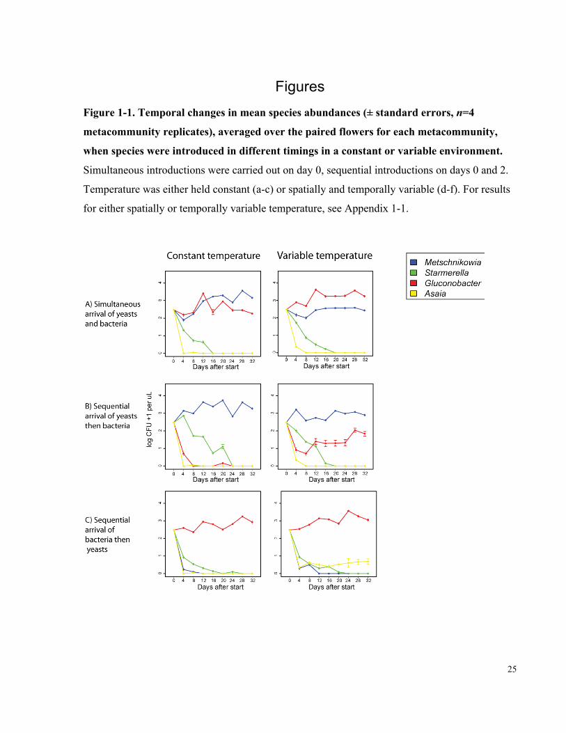
25
Figures
Figure 1-1. Temporal changes in mean species abundances (± standard errors, n=4
metacommunity replicates), averaged over the paired flowers for each metacommunity,
when species were introduced in different timings in a constant or variable environment.
Simultaneous introductions were carried out on day 0, sequential introductions on days 0 and 2.
Temperature was either held constant (a-c) or spatially and temporally variable (d-f). For results
for either spatially or temporally variable temperature, see Appendix 1-1.

26
Figure 1-2. Characterization of the common species Metschnikowia reukaufii and
Gluconobacter sp.
(a) Effect on mean nectar pH after 36 hours growth (± standard errors, n= 3), (b) Percent decline
in amino acid concentrations in nectar after 36 hours growth (± standard errors, n= 3), (c) Mean
abundance attained after four days of growth at different temperatures
!"
#"
$"
%"
&"
'"
("
)*+,-*." !"#$%&'()*+(,- ./0%*'*1,%#"2-
!"#$%&'()
*("#+",'#-.$-&"/'+0'0"#$%&'
/!0$'"
/!0$"
/!0#'"
/!0#"
/!0!'"
!")*+,-*."
1"&#"0$%2"'/"#.+0"'+0'%3+04'%#+/#40#"0$&%$+40567'
!"#$%&'()*+(,- ./0%*'*1,%#"2-
*("#+",'#-.$-&"/'+0'0"#$%&'!"
!0'"
#"
#0'"
$"
$0'"
%"
%0'"
'" #%" $#" $1" %%"
89-0/%0#"'%:$"&';</%='+0#-9%$+40'5.42>?5@ABC-.'0"#$%&'D>7''
E"3("&%$-&"'54@7'
./0%*'*1,%#"2-!"#%&'()*+(,-
*("#+",
3 4 5
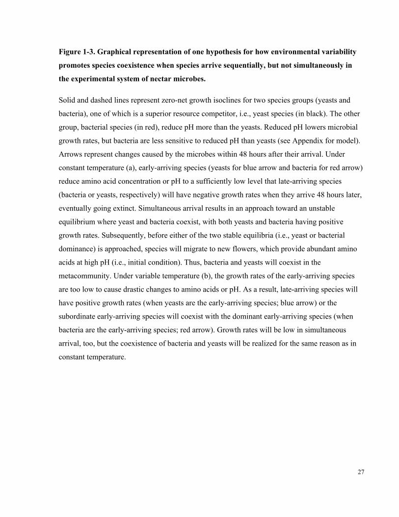
27
Figure 1-3. Graphical representation of one hypothesis for how environmental variability
promotes species coexistence when species arrive sequentially, but not simultaneously in
the experimental system of nectar microbes.
Solid and dashed lines represent zero-net growth isoclines for two species groups (yeasts and
bacteria), one of which is a superior resource competitor, i.e., yeast species (in black). The other
group, bacterial species (in red), reduce pH more than the yeasts. Reduced pH lowers microbial
growth rates, but bacteria are less sensitive to reduced pH than yeasts (see Appendix for model).
Arrows represent changes caused by the microbes within 48 hours after their arrival. Under
constant temperature (a), early-arriving species (yeasts for blue arrow and bacteria for red arrow)
reduce amino acid concentration or pH to a sufficiently low level that late-arriving species
(bacteria or yeasts, respectively) will have negative growth rates when they arrive 48 hours later,
eventually going extinct. Simultaneous arrival results in an approach toward an unstable
equilibrium where yeast and bacteria coexist, with both yeasts and bacteria having positive
growth rates. Subsequently, before either of the two stable equilibria (i.e., yeast or bacterial
dominance) is approached, species will migrate to new flowers, which provide abundant amino
acids at high pH (i.e., initial condition). Thus, bacteria and yeasts will coexist in the
metacommunity. Under variable temperature (b), the growth rates of the early-arriving species
are too low to cause drastic changes to amino acids or pH. As a result, late-arriving species will
have positive growth rates (when yeasts are the early-arriving species; blue arrow) or the
subordinate early-arriving species will coexist with the dominant early-arriving species (when
bacteria are the early-arriving species; red arrow). Growth rates will be low in simultaneous
arrival, too, but the coexistence of bacteria and yeasts will be realized for the same reason as in
constant temperature.
28
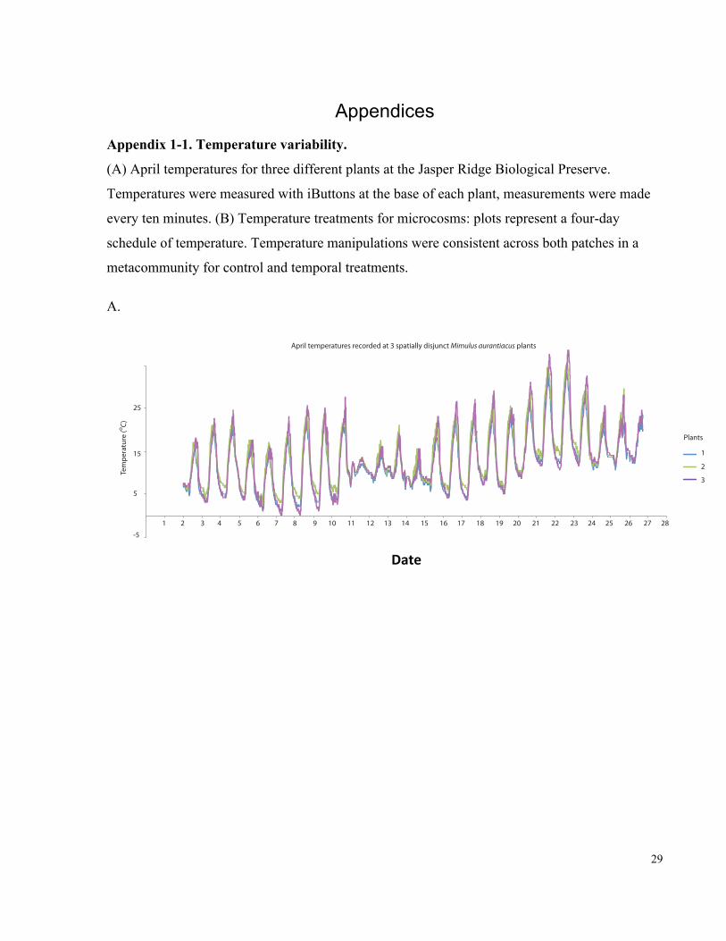
29
Appendices
Appendix 1-1. Temperature variability.
(A) April temperatures for three different plants at the Jasper Ridge Biological Preserve.
Temperatures were measured with iButtons at the base of each plant, measurements were made
every ten minutes. (B) Temperature treatments for microcosms: plots represent a four-day
schedule of temperature. Temperature manipulations were consistent across both patches in a
metacommunity for control and temporal treatments.
A.
1 2 3 4 5 6 7 8 9 10 11 12 13 14 15 16 17 18 19 20 21 22 23 24 25 26 27 28
Tem
pera
ture
(o C)
Date
5
15
25
-5
April temperatures recorded at 3 spatially disjunct Mimulus aurantiacus plants
Plants
1
2
3
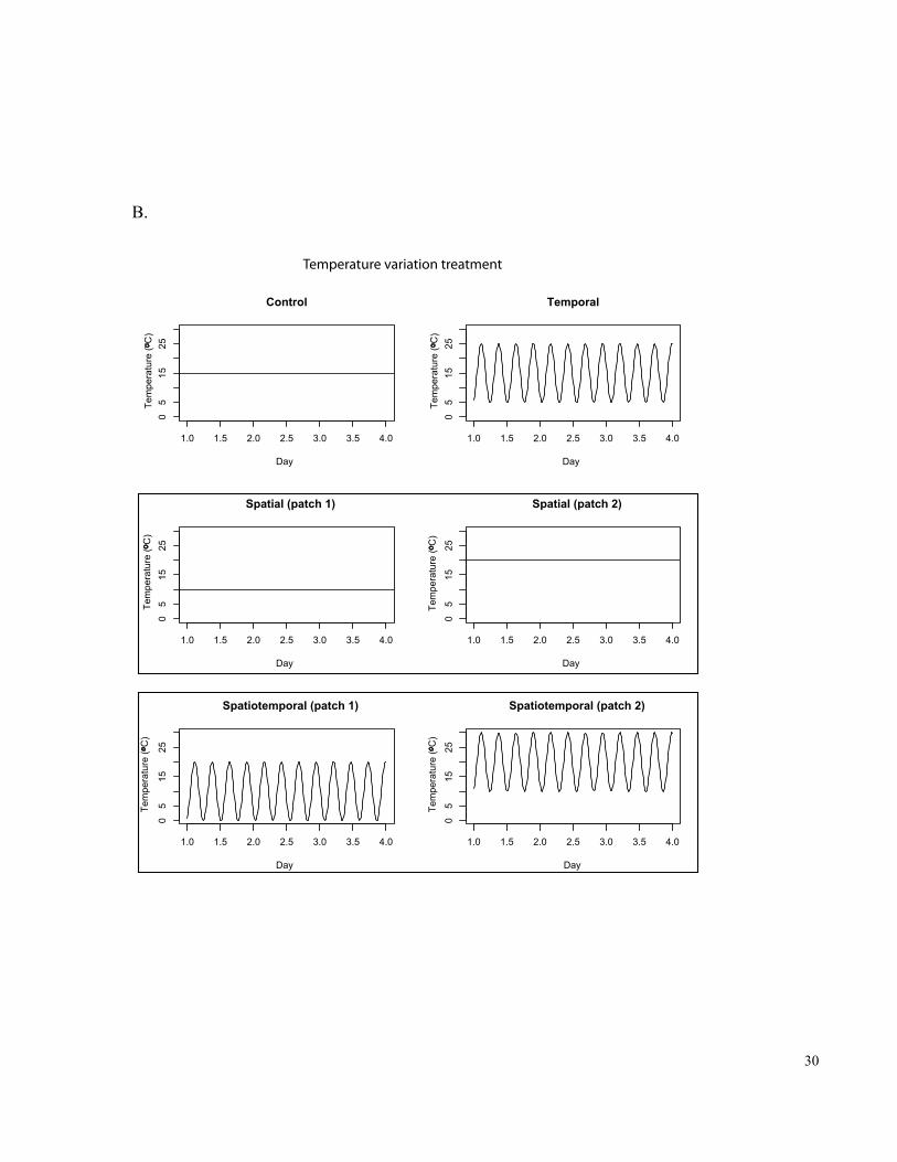
30
B.
1.0 1.5 2.0 2.5 3.0 3.5 4.0
05
1525
Control
Day
Temperature (oC)
1.0 1.5 2.0 2.5 3.0 3.5 4.00
515
25
Temporal
Day
Temperature (oC)
1.0 1.5 2.0 2.5 3.0 3.5 4.0
05
1525
Spatial (patch 1)
Day
Temperature (oC)
1.0 1.5 2.0 2.5 3.0 3.5 4.0
05
1525
Spatial (patch 2)
Day
Temperature (oC)
1.0 1.5 2.0 2.5 3.0 3.5 4.0
05
1525
Spatiotemporal (patch 1)
Day
Temperature (oC)
1.0 1.5 2.0 2.5 3.0 3.5 4.0
05
1525
Spatiotemporal (patch 2)
Day
Temperature (oC)
Temperature variation treatment

31
Appendix 1-2. Temporal changes in mean species abundances when species were
introduced in different arrival timings with either spatial or temporal environmental
(temperature) variability. Symbols are as in Figure 1-1.

32
Appendix 1-3. Consumer-resource model used to produce zero-net growth isoclines
(ZNGIs), modelling competition for resources (amino acids) between a bacteria species
(representing Gluconobacter) producing an inhibitor (pH) and a yeast species (representing
Metschnikowia).
€
dYdt
=Y[t]* (µY ,T A[t]
(KY + A[t])(1+pH[t]KpHY
)−m)
dBdt
= B[t]* (µB ,T A[t]
(KB + A[t])(1+pH[t]KpHB
)−m)
dAdt
= −QYY[t]µY ,T A[t]
(KY + A[t])(1+pH[t]KpHY
)−
QBB[t]µB ,T A[t]
(KB + A[t])(1+pH[t]KpHB
)
dpHdt
=εBB[t]µB ,T A[t]
(KB + A[t])(1+pH[t]KpHB
)
Where: Y - the dominant yeast species, Metschnikowia;
B - the dominant acetic acid bacteria species, Gluconobacte
µi,T - maximum growth rate at a given temperature
A – concentration of amino acids in the medium
pH – medium pH
Ki – half saturation constant for species i on amino acids
KpHi – resistance to pH – pH at which growth is ½ maximum
Qi – units of amino acids used to produce one unit species i
εi – units inhibitor produced per unit of species i (in this case, only Bacteria produce inhibitor).
m – mortality rate

33
Chapter 2 Community-level interactions alter species responses to climate
change
2 2
2.1 Abstract
One of the most apparent impacts of climate change is the shift in the timing of phenological
events such as fruiting and flowering in plant communities. The sensitivity of phenology to
climatic cues makes it useful as an indicator of the effects of warming, but long-term studies of
phenological shifts suggest that there is much variation within and between communities in the
extent of shifts. Such variation makes understanding and predicting community effects difficult.
One explanation for this variation is that most studies ignore interactions between temperature
and the competitive environment a species faces. Competition can create seasonal constraints on
resource availability that impact the timing of life history events. We use simulation models to
show how coupling temperature increases with interspecific competition can alter expectations
for phenological shifts in annual plant communities.
We found that interspecific competition introduced variation between communities and among
species within communities in how the timing of flowering shifted with warming. High
interspecific competition constrained the extent of phenological shifts in communities. Within
communities, species which avoid competition temporally (e.g. winter annuals) and large,
competitive late season species advanced most consistently with warming, while midseason
species advanced less than expected. Mismatches between the optimal timing of flowering and
rates of development were another outcome of warming that introduced variability in observed
dates of flowering onset. Considering that competition is one of many biotic interactions species
experience, ignoring the biotic environment is likely to reduce the predictability of changes in
communities with climate change.
34
2.2 Introduction
Global climate change has had demonstrable impacts on the timing of biological events (Menzel
et al. 2006; Schwartz et al. 2006; Parmesan 2007; Primack & Miller-Rushing 2012). Changes in
the timing of life history (phenology) events can have ecosystem-wide implications, including
changes in net primary productivity (Nemani et al. 2003; Edwards & Richardson 2004), CO2
cycles (Keeling et al. 1996), and disrupted species interactions (Tylianakis et al. 2008). The
primary evidence for the potential impact of climate change has been from controlled warming
experiments on single populations (with exceptions, see Sherry et al. (2006)), but recent papers
have revealed just how variable phenology shifts can be in natural communities (Diez et al.
2012; Wolkovich et al. 2012). Numerous ecological processes and interactions influence
phenology in communities.
Research examining biotic interactions with warming-induced phenological shifts has largely
focused on trophic mismatches, such as between plants and pollinator or herbivore communities
(Edwards & Richardson 2004; Parmesan 2006; e.g. Post & Forchhammer 2008; Diez et al.
2012). Yet, competitive interactions are ubiquitous in plant communities (Keddy 1989) and
given that competition can reduce growth rates, reproductive output and increase flowering time
(Lovett Doust & Lovett Doust 1988; Reekie & Bazzaz 2005), it is reasonable that competitive
interactions can influence phenological responses to warming. Given the dearth of community
warming experiments, the question of how within-trophic level competitive interactions might
interact with increasing temperatures has not been considered.
Competition can reduce nutrient uptake and ultimately limit or alter the timing of allocation to
reproduction in annual plants (Weiner 1982, 1988; Weiner & Damgaard 2006). Species may
have a threshold size that determines the onset of reproductive, or alternately important
environmental cues might drive reproductive allocation, with allocation being proportional to
size (Lacey 1986; Weiner 1988; Bernier & Perilleux 2005). The staggered nature of community-
level patterns in flowering phenology suggests a potential strategy for minimizing competition
between species is the partitioning of growth and development into temporal niches with
minimal overlap. As a result, environmentally induced shifts in phenology can alter the duration
or frequency of competitive interactions throughout the community. In turn, potential
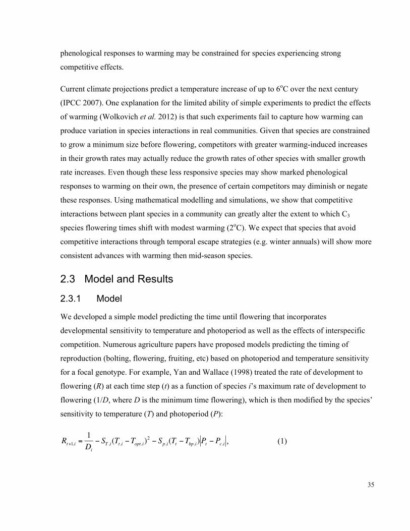
35
phenological responses to warming may be constrained for species experiencing strong
competitive effects.
Current climate projections predict a temperature increase of up to 6oC over the next century
(IPCC 2007). One explanation for the limited ability of simple experiments to predict the effects
of warming (Wolkovich et al. 2012) is that such experiments fail to capture how warming can
produce variation in species interactions in real communities. Given that species are constrained
to grow a minimum size before flowering, competitors with greater warming-induced increases
in their growth rates may actually reduce the growth rates of other species with smaller growth
rate increases. Even though these less responsive species may show marked phenological
responses to warming on their own, the presence of certain competitors may diminish or negate
these responses. Using mathematical modelling and simulations, we show that competitive
interactions between plant species in a community can greatly alter the extent to which C3
species flowering times shift with modest warming (2oC). We expect that species that avoid
competitive interactions through temporal escape strategies (e.g. winter annuals) will show more
consistent advances with warming then mid-season species.
2.3 Model and Results
2.3.1 Model
We developed a simple model predicting the time until flowering that incorporates
developmental sensitivity to temperature and photoperiod as well as the effects of interspecific
competition. Numerous agriculture papers have proposed models predicting the timing of
reproduction (bolting, flowering, fruiting, etc) based on photoperiod and temperature sensitivity
for a focal genotype. For example, Yan and Wallace (1998) treated the rate of development to
flowering (R) at each time step (t) as a function of species i’s maximum rate of development to
flowering (1/D, where D is the minimum time flowering), which is then modified by the species’
sensitivity to temperature (T) and photoperiod (P):
€
Rt+1,i =1Di
− ST ,i(Tt,i −Topt ,i)2 − Sp,i(Tt −Tbp,i)Pt − Pc,i , (1)

36
where Topt and Pc are the species’ optimal temperature and critical photoperiod, and St and Sp are
the sensitivity of the species to non-optimal temperatures and photoperiods. High sensitivity
suggests that when temperature and/or photoperiod diverge from optimal, the species’ rate of
development slows greatly compared to a more tolerant, insensitive species. This model assumes
that supraoptimal temperatures have a negative effect on development (Craufurd & Wheeler
2009), however other relationships between temperature and development could be modelled.
Under optimal temperatures and photoperiods, a species’ rate of development to flowering
should approach its maximum.
Species necessarily face limitations on the resources available to allocate to growth and
reproduction (Reznick 1985; Obeso 2002). Spatially and temporally contemporaneous species
compete for resources, and this can affect their growth and development (Weiner 1988). For
example, there is a well known “law of constant yield” which states that above a certain density,
no further gains in yield can be obtained due to the negative effects of intraspecific competition
(Weiner & Freckleton 2010). Because most models of development are formulated for crop
species where interspecific competition is minimized, interspecific competition is generally not
incorporated into models of reproductive timing for agricultural species.
To incorporate interspecific competition into Equation 1, we make the simplifying assumption
that that competition is a function of size: in particular, size asymmetries with competitors will
affect the magnitude and direction of species’ interactions (Weiner & Damgaard 2006). We
model biomass accumulation (M) over each time step (t) as a logistic function, where the
denominator includes a term representing the competitive environment (here, C, some measure
of competitive intensity, scaled by the mass of each competitor). The term C represents the
intensity of competition, for example, in relation to the proportion of niche overlap between
species i and species j (and resulting decline in growth rate when they co-occur). Competition is
therefore a declining function of species i’s size (i.e. CM). p is the innate rate of biomass
accumulation, θ represents a self-thinning constant (e.g. Weis & Hochberg 2000; Weiner &
Damgaard 2006).
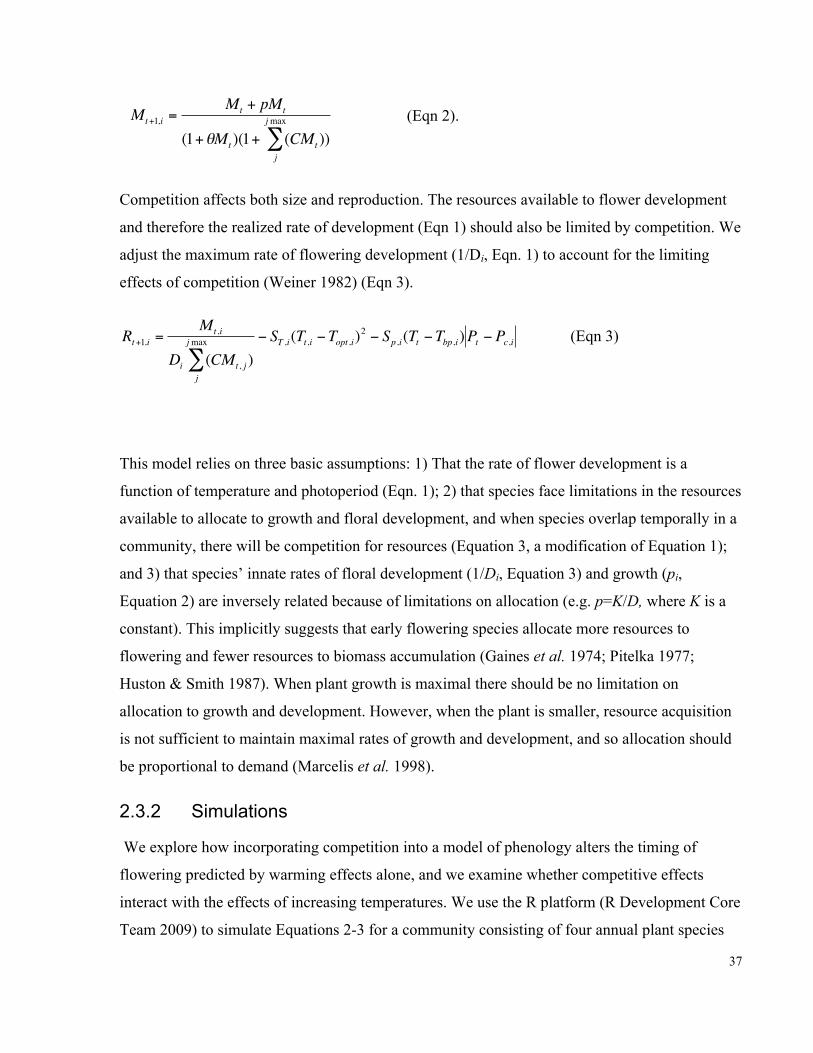
37
€
Mt+1,i =Mt + pMt
(1+θMt )(1+ (CMt )j
jmax
∑ ) (Eqn 2).
Competition affects both size and reproduction. The resources available to flower development
and therefore the realized rate of development (Eqn 1) should also be limited by competition. We
adjust the maximum rate of flowering development (1/Di, Eqn. 1) to account for the limiting
effects of competition (Weiner 1982) (Eqn 3).
€
Rt+1,i =Mt ,i
Di (CMt , j )j
jmax
∑− ST ,i(Tt,i −Topt ,i)
2 − Sp,i(Tt −Tbp,i)Pt − Pc,i (Eqn 3)
This model relies on three basic assumptions: 1) That the rate of flower development is a
function of temperature and photoperiod (Eqn. 1); 2) that species face limitations in the resources
available to allocate to growth and floral development, and when species overlap temporally in a
community, there will be competition for resources (Equation 3, a modification of Equation 1);
and 3) that species’ innate rates of floral development (1/Di, Equation 3) and growth (pi,
Equation 2) are inversely related because of limitations on allocation (e.g. p=K/D, where K is a
constant). This implicitly suggests that early flowering species allocate more resources to
flowering and fewer resources to biomass accumulation (Gaines et al. 1974; Pitelka 1977;
Huston & Smith 1987). When plant growth is maximal there should be no limitation on
allocation to growth and development. However, when the plant is smaller, resource acquisition
is not sufficient to maintain maximal rates of growth and development, and so allocation should
be proportional to demand (Marcelis et al. 1998).
2.3.2 Simulations
We explore how incorporating competition into a model of phenology alters the timing of
flowering predicted by warming effects alone, and we examine whether competitive effects
interact with the effects of increasing temperatures. We use the R platform (R Development Core
Team 2009) to simulate Equations 2-3 for a community consisting of four annual plant species
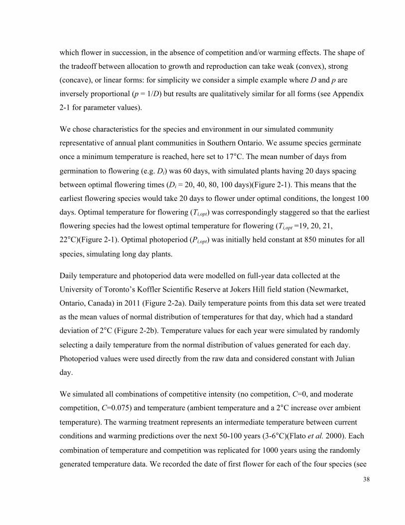
38
which flower in succession, in the absence of competition and/or warming effects. The shape of
the tradeoff between allocation to growth and reproduction can take weak (convex), strong
(concave), or linear forms: for simplicity we consider a simple example where D and p are
inversely proportional (p = 1/D) but results are qualitatively similar for all forms (see Appendix
2-1 for parameter values).
We chose characteristics for the species and environment in our simulated community
representative of annual plant communities in Southern Ontario. We assume species germinate
once a minimum temperature is reached, here set to 17°C. The mean number of days from
germination to flowering (e.g. Di) was 60 days, with simulated plants having 20 days spacing
between optimal flowering times (Di = 20, 40, 80, 100 days)(Figure 2-1). This means that the
earliest flowering species would take 20 days to flower under optimal conditions, the longest 100
days. Optimal temperature for flowering (Ti,opt) was correspondingly staggered so that the earliest
flowering species had the lowest optimal temperature for flowering (Ti,opt =19, 20, 21,
22°C)(Figure 2-1). Optimal photoperiod (Pi,opt) was initially held constant at 850 minutes for all
species, simulating long day plants.
Daily temperature and photoperiod data were modelled on full-year data collected at the
University of Toronto’s Koffler Scientific Reserve at Jokers Hill field station (Newmarket,
Ontario, Canada) in 2011 (Figure 2-2a). Daily temperature points from this data set were treated
as the mean values of normal distribution of temperatures for that day, which had a standard
deviation of 2°C (Figure 2-2b). Temperature values for each year were simulated by randomly
selecting a daily temperature from the normal distribution of values generated for each day.
Photoperiod values were used directly from the raw data and considered constant with Julian
day.
We simulated all combinations of competitive intensity (no competition, C=0, and moderate
competition, C=0.075) and temperature (ambient temperature and a 2°C increase over ambient
temperature). The warming treatment represents an intermediate temperature between current
conditions and warming predictions over the next 50-100 years (3-6°C)(Flato et al. 2000). Each
combination of temperature and competition was replicated for 1000 years using the randomly
generated temperature data. We recorded the date of first flower for each of the four species (see

39
Appendix 2-2 for R code) and looked at changes in the mean flowering date over 1000 replicate
years using a two-way ANOVA with a Poisson distribution.
2.3.3 Results
In the absence of warming and competitive interactions among species, the four plant species
flowered in a temporally staggered manner in the order predicted by their rates of reproductive
allocation (average Julian day: µ1=138.7, µ2=159.9, µ3=201.8, µ4=223.2) (Figure 2-3, light blue).
Under ambient conditions, but with competition incorporated into predicted date of first
flowering, the average date of flowering was delayed for all four species, but proportionally
more for early (e.g. species 1 and 2) species (average Julian day: µ1=158.2, µ2=220.9, µ3=227.3,
µ4=227.7)(Figure 2-3, dark blue).
Under warming conditions, the timing of flowering advances, because temperatures become
suitable for germination and rapid development earlier in the year. In the absence of competition,
flowering dates are much advanced (average Julian day: µ1=121.6, µ2=143.3, µ3=185.8,
µ4=207.5)(Figure 2-3, pink). When species face both competitive interactions (and therefore
restrictions on resources) in addition to warming conditions, flowering dates are advanced.
However, this advance is less, particularly for mid-season plants (species 2, 3): Average Julian
days were µ1=141.4, µ2=208.2, µ3=211.3, µ4=211.4, respectively (Figure 2-3, red).
For all four species, the mean date of first flower occurred significantly earlier under warming
conditions and was significantly delayed when competition was present (p<0.001). For species 1,
2 and 3 there was also a significant interaction (p<0.05) between the warming conditions and the
presence of competition, while the interaction was not significant for species 4. Species 2
exhibited greater delays in flowering than expected (~4 days) when there was both competition
and 2°C warming present, while species 1 & 3 faced modest but significant delays (<1 day on
average) in the presence of both warming and competition.
There are two mechanisms by which competition between species can increase in this model –
the intensity of competition (the term C in equations 2 & 3) can increase, or the duration of
competitive interactions can increase. The latter situation would be expected when species have
high temporal overlap, while the former would reflect greater niche (e.g. resource use) overlap
40
between species. Increased duration of overlap should have a greater effect on species that have
a temporal escape strategy and are poor competitors (e.g. early season species such as species 1;
Figure 2-4). In Figure 4, as temporal overlap between species increases (x-axis values become
smaller), competition increases and early species are greatly delayed in flowering.
It is also notable that the distribution of flowering dates changes between the ambient
temperature simulations and the warming simulations. The distributions are significantly right-
skewed (p<0.05) under ambient conditions, and bimodal under warming conditions. Variance
tests of the distribution of flowering dates between ambient and warmed treatments (for each
species, comparing the treatments where competition is present and where competition is absent
separately) showed that in every case variance was greater (p<0.01) when there was warming
(Figure 2-5).
2.4 Discussion
Given the fact that phenological measures are an important indicator of climate change,
understanding how community interactions affect phenology is a critically important goal.
Variability within phenological data tends to be high (Diez et al. 2012), with different responses
being observed among populations (Schwartz & Hanes 2009), among species within a
community, (Cleland et al. 2006; Miller-Rushing & Primack 2008; Crimmins et al. 2010) and
among communities (Aldridge et al. 2011). Our results suggest two possible ways in which
competitive interactions can contribute to this variability. First, phenological responses may
differ among habitats or populations if there are differences in the strength of competitive
interactions. Secondly, even within habitats, different species may show differing responses to
warming based on changes in the importance of competitive interactions and their ability to
compete.
If competition between species is an important contributor to variation in flowering time, we can
generate a few hypotheses about how to search for this signal in long-term data sets. Habitats
where competition is high among annual plants, due to low habitat heterogeneity or similar niche
requirements among species, high species richness, or short growing seasons (e.g. Hovenden et
al. 2008), might be predicted to show smaller phenological shifts with warming climate. In
contrast, agricultural systems—in which competition is suppressed—typically provide some of
41
the strongest evidence of advancing flowering times (Estrella et al. 2007; Craufurd & Wheeler
2009). Other natural systems characterized by relatively low densities or richness (e.g.,
frequently disturbed or stressful habitats) should also experience greater shifts in flowering time
compared to more diverse, stable ecosystems. For example, in a meta-analysis of arctic
phenological shifts with experimental warming, greater advances in bud-burst and antithesis
were seen in the high arctic compared to lower arctic locations (Arft et al. 1999).
Within habitats, the model results suggest that species that reduce competition by early and rapid
completion of their life cycle (such as winter annuals) and large, late-season annuals should be
less constrained by competition than species that flower at intermediate dates and sizes. Such
mid-season species face increasing overlap with fast growing, late season species as temperatures
warm, increasing competitive duration and intensity, ultimately reducing their developmental
rates. Certainly early flowering annuals are among the species for which advances with warming
are most consistently observed (Price & Waser 1998; Kudo et al. 2004; Sherry et al. 2006).
Our model is meant to be a general representation of the effects of competition on phenological
variables such as the timing of flowering onset, and as such we make simplifying assumptions
about the relationship between growth and reproduction. The strength and shape of the tradeoff
between growth and reproduction greatly affects our results: differential interactions of
competition and warming depend on a tradeoff between development and growth, and as the
tradeoff weakens, species should be similarly effected by warming regardless of the timing of
their development. We assume that allocation to growth and reproduction are continuous
processes from germination onwards: this may not be accurate, as it is also possible that
reproductive allocation requires a minimum size to begin. In addition, we assume that
competition is the most important constraint on development that species will experience.
Competition has been shown numerous times to be important for plants (Connell 1983; Levine &
Rees 2002; Silvertown 2004). However, other biotic interactions may act as important
constraints on flowering time. For example, we assumed that pollinators were not limiting in our
simulated community, but the availability of pollinators can be an important temporal constraint
on flowering time in some systems (e.g. Rathcke & Lacey 1985; Kochmer & Handel 1986).
Perennial species are not considered, as their lifecycles are considerably more complicated and
42
development, flowering, and competition may occur in relation to conditions that exceed a single
year’s climate (e.g. Tucker & Cadotte In Press).
We considered a relatively moderate increase in climate (2°C) representing temperatures likely
to be experienced by plants in Southern Ontario as climates warm, but temperature increases
greater than 3-6°C are predicted for 2100 (Flato et al. 2000), suggesting that pressure to flower
earlier will be strong. Results are qualitatively similar when we consider a 4°C increase in
temperature, but advances in flowering time and the size of the interaction between competition
and warming are increased. This increases the pressure to flower earlier and the competitive
constraints on doing so for mid-season plants. Models of warming for the region often predict
greater increases in temperature for winter and early spring months, such a pattern is likely to
increase the size of the interaction between warming and competition for early season species.
An important question regarding annual plants’ responses to warming temperatures is whether
species possess sufficient phenotypic plasticity or the capacity to adapt rapidly to maintain
fitness under changing conditions. With either phenotypic plasticity or rapid adaptation, plants
are able to explore phenotypic space in the absence of competitors. However, competition can
create evolutionary constraints limiting the actual rate of evolutionary change (Futuyma 2010),
and this would be the case in our model system if advanced flowering proves costly when
competitors are present. These competition constraints can be further confounded by herbivore or
pollinator timing, resulting in higher fitness consequences for shifting phenology and thus
making it difficult to predict how optimal flowering should evolve (Elzinga et al. 2007). Thus,
species could maintain suboptimal fitness, despite the ability to take advantage of a warming
climate.
One interesting outcome of our simulations was the change in the distribution of flowering times
between ambient and warming conditions. Changes in skew arise under ambient conditions,
where species typically flower close to their optimal temperatures. Occasional warm years shift
flowering times to earlier in the season, resulting in a right-skewed distribution, but overall
optimal flowering temperatures and flowering rates are in agreement, consistent with adaptive
timing seen in plants. However under warming conditions species’ optimal temperatures and
rates of development are mismatched: species may experience temperatures beyond their optima
43
during the growing season, creating periods of slow development. As a result, a bimodal
distribution emerges, such that species either manage to complete development prior to
experiencing detrimental temperatures, or else are delayed in the timing of flowering.
Supraoptimal temperatures have been shown to cause delays in crop species (i.e. “heat delay”)
(Craufurd & Wheeler 2009; Thomas et al. 2010). Sherry et al. (2006) similarly found that some
mid-season species faced delays, likely in response to high temperatures mid-summer. This
increased variability in species’ flowering time is likely to magnify trophic mismatches with
pollinator or herbivore communities. It also suggests one additional explanation for variation in
observational studies.
Warming temperatures are already being shown to have ecosystem-wide effects, and changes in
biotic communities will change in response to warming conditions helps us predict how
biodiversity, ecosystem services, carbon balance, pollination services and crop success, and
species invasions will change. Our analysis provides a plausible mechanism in which
competitive interactions alone can explain variation in warming-induced phenological responses
between and within communities. Many additional factors likely contribute to this variation,
including herbivory and resource limitation, intraspecific variation, phenotypic plasticity, and
differences in mating systems (Diez et al. 2012). However, given the general ubiquity of
competition shaping plant communities (Levine & HilleRisLambers 2009), our results suggest
that climate change-induced phenological shifts cannot be fully understood without accounting
for competition. Future studies need to experimentally manipulate the strength of intra- and
interspecific competitive interactions in plant communities and consider how these treatments
alter community responses to warming conditions.
2.5 Acknowledgements
Thanks to Art Weis and Kelly Carscadden for comments on an earlier version of this manuscript.

44
References
Aldridge G., Inouye D.W., Forrest J., Barr W.A. & Miller-Rushing A.J. (2011). Emergence of a mid-season period of low floral resources in montane meadow ecosystem associated with climate change. Journal of Ecology, 99, 905-913.
Arft A., Walker M., Gurevitch J.e.a., Alatalo J., Bret-Harte M., Dale M., Diemer M., Gugerli F., Henry G. & Jones M. (1999). Responses of tundra plants to experimental warming: meta-analysis of the international tundra experiment. Ecological Monographs, 69, 491-511.
Bernier G. & Perilleux C. (2005). A physiological overview of the genetics of flowering time control. Plant Biotechnology Journal, 3, 3-16.
Cleland E., Chiariello S.R., Loarie S.R., Mooney H.A. & Field C.B. (2006). Diverse responses of phenology to global changes in a grassland ecosystem. Proceedings of the National Academy of Science, 103, 13740-13744.
Connell J.H. (1983). On the prevalence and relative importance of interspecific competition: evidence from field experiments. The American Naturalist, 122, 661-696.
Craufurd P.Q. & Wheeler T.R. (2009). Climate change and the flowering time of annual crops. Journal of Experimental Botany, 60, 2529-2539.
Crimmins T.M., Crimmins M.A. & Bertelsen C.D. (2010). Complex responses to climate drivers in onset of spring flowering across a semi-arid elevation gradient. Journal of Ecology, 98, 1042-1051.
Diez J.M., Ibanez I., Miller-Rushing A.J., Mazer S.J., Crimmins T.M., Crimmins M.A., Bertelsen C.D. & Inouye D.W. (2012). Forecasting phenology: from species variability to community patterns. Ecology Letters, 15, 545-553.
Edwards M. & Richardson A.J. (2004). Impact of climate change on marine pelagic phenology and trophic mismatch. Nature, 430, 881-884.
Elzinga J.A., Atlan A., Biere A., Gigord L., Weis A.E. & Bernasconi G. (2007). Time after time: flowering phenology and biotic interactions. Trends in Ecology & Evolution, 22, 432-439.
Estrella N., Sparks T.H. & Menzel A. (2007). Trends and temperature response in the phenology of crops in Germany. Global Change Biology, 13, 1737-1747.
Flato G.M., Boer G.J., Lee W.G., McFarlane N.A., Ramsden D., Reader M.C. & Weaver A.J. (2000). The Canadian Centre for Climate Modelling and Analysis global coupled model and its climate. Climate Dynamics, 16, 451-467.
Futuyma D.J. (2010). Evolutionary constraint and ecological consequences. Evolution, 64, 1865-1884.
Gaines M.S., Vogt K.J., Hamrick J.L. & Caldwell J. (1974). Reproductive strategies and growth patterns in sunflowers (Helianthus). American Naturalist, 108, 889-894.
45
Hovenden M.J., Wills K.E., Vander Schoor J.K., Williams A.L. & Newton P.C. (2008). Flowering phenology in a species rich temperate grassland is sensitive to warming but not elevated CO2. New Phytologist, 178, 815-822.
Huston M.A. & Smith T. (1987). Plant succession: life history and competition. The American Naturalist, 130, 169-198.
Keddy P.A. (1989). Competition. 2nd edn. Springer.
Keeling C.D., Chin J. & Whorf T. (1996). Increased activity of northern vegetation inferred from atmospheric CO2 measurements. Nature, 382, 146-149.
Kochmer J.P. & Handel S.N. (1986). Constraints and Competition in the Evolution of Flowering Phenology. Ecological Monographs, 56, 303-325.
Kudo G., Nishikawa Y., Kasagi T. & Kosuge S. (2004). Does seed production of spring ephemerals decrease when spring comes early? Ecological Research, 19, 255-259.
Lacey E.P. (1986). Onset of reproduction in plants: size-versus age-dependency. Trends in Ecology & Evolution, 1, 72-75.
Levine J.M. & HilleRisLambers J. (2009). The importance of niches for the maintenance of species diversity. Nature, 461, 254-257.
Levine J.M. & Rees M. (2002). Coexistence and relative abundance in annual plant assemblages: The roles of competition and colonization. The American Naturalist, 160, 452-467.
Lovett Doust J. & Lovett Doust L. (eds.) (1988). Plant reproductive ecology: patterns and strategies. Oxford University Press, Oxford.
Marcelis L.F.M., Heuvelink E. & Goudriaan J. (1998). Modelling biomass production and yield of horticultural crops: a review. Scientia Horticulturae, 75, 83-111.
Menzel A., Sparks T.H., Estrella N., Koch E., Aasa A., Ahas R., Almakubler K., Bissolli P., Braslavskov, O. & Briede A. (2006). European phenological response to climate change matches the warming pattern. Global Change Biology, 12, 1969-1976.
Miller-Rushing A.J. & Primack R.B. (2008). Global warming and flowering times in Thoreau's Concord: a community perspective. Ecology, 96, 1821-1829.
Nemani R.R., Keeling C.D., Hashimoto H., Jolly W.M., Piper S.C., Tucker C.J., Myneni R.B. & Running S.W. (2003). Climate-driven increases in global terrestrial net primary production from 1982 to 1999. Science, 300, 1560-1563.
Obeso J.R.N. (2002). Tansley Review No. 139. The Costs of Reproduction in Plants. New Phytologist, 155, 321-348.
Parmesan C. (2006). Ecological and evolutionary responses to recent climate change. Annual Review of Ecology, Evolution, and Systematics, 37, 637-669.
Parmesan C. (2007). Influences of species, latitude and methodologies on estimates of phenological response to global warming. Global Change Biology, 13, 1860-1872.
Pitelka L.F. (1977). Energy allocation in annual and perennial lupines (Lupinus: Leguminosae). Ecology, 58, 401-420.

46
Post E. & Forchhammer M.C. (2008). Climate change reduces reproductive success of an Arctic herbivore through trophic mismatch. Philosophical Transactions of the Royal Society B: Biological Sciences, 363, 2367-2373.
Price M.V. & Waser N.M. (1998). Effects of experimental warming on plant reproductive phenology in a subalpine meadow. Ecology, 79, 1261-1271.
Primack R.B. & Miller-Rushing A.J. (2012). Uncovering, collecting, and analyzing records to investigate the ecological impacts of climate change: a template from Thoreau's Concord. Bioscience, 62, 170-181.
R Development Core Team (2009). R: A Language and Environment for Statistical Computing. R Foundation for Statistical Computing. Vienna, Austria.
Rathcke B. & Lacey E.P. (1985). Phenological Patterns of terrestrial plants. Annual Review of Ecology and Systematics, 16, 179-214.
Reekie E.G. & Bazzaz F.A. (eds.) (2005). Reproductive allocation in plants. Elsevier Academic Press, Oxford, UK.
Reznick D. (1985). Cost of reproduction: an evaluation of the empirical evidence. Oikos, 44, 257-267.
Schwartz M.D., Ahas R. & Aasa A. (2006). Onset of spring starting earlier across the Northern Hemisphere. Global Change Biology, 12, 343-351.
Schwartz M.D. & Hanes J.M. (2009). Continental-scale phenology: warming and chilling. International Journal of Climatology, 30, 1595-1598.
Sherry R.A., Zhou X., Gu S., Arnone III J.A., Schimel D.S. & Verburg P.S. (2006). Divergence of reproductive phenology under climate warming. Proceedings of the National Academy of Sciences of the United States of America.
Silvertown J. (2004). Plant coexistence and the niche. Trends in Ecology and Evolution, 19, 605-611.
Thomas M.G., Boote K.J., Pan D. & Allen L.H. (2010). Elevated temperature delays onset of reproductive growth and reduces seed growth rate of soybean. Journal of Agro Crop Science, 1(1).
Tucker C.M. & Cadotte M.W. (In Press). Fire variability, as well as frequency, can explain coexistence between seeder and resprouter life histories. Journal of Applied Ecology.
Tylianakis J.M., Didham R.K., Bascompte J. & Wardle D.A. (2008). Global change and species interactions in terrestrial ecosystems. Ecology Letters, 11, 1351-1363.
Weiner J. (1982). A neighbourhood model of annual-plant interference. Ecology, 63, 1237-1241.
Weiner J. (1988). The influence of competition on plant reproduction. In: Plant Reproductive Ecology (eds. Doust JL & Lovett Doust L). Oxford University Press Oxford.
Weiner J. & Damgaard C. (2006). Size-asymmetric competition and size-asymmetric growth in a spatially explicit zone-of-influence model of plant competition. Ecological Research, 21, 707-712.
47
Weiner J. & Freckleton R.P. (2010). Constant final yield. Annual Review of Ecology, Evolution, and Systematics, 41, 173-192.
Weis A.E. & Hochberg M.E. (2000). The diverse effects of intraspecific competition on the selective advantage to resistance: a model and its predictions. The American Naturalist, 156, 276-292.
Wolkovich E.M., Cook B.I., Allen J.M., Crimmins T.M., Betancourt J.L., Travers S.E., Pau S., Regetz J., Davies T.J., Kraft N.J.B., Ault T.R., Bolmgren K., Mazer S.J., McCabe G.J., McGill B., Parmesan C., Salamin N., Schwartz M.D. & Cleland E. (2012). Warming experiments underpredict plant phenological responses to climate change. Nature, 485, 494-497.
Yan W. & Wallace D.H. (1998). Simulation and prediction of plant phenology for five crops based on photoperiod x temperature interaction. Annals of Botany, 81, 705-716.
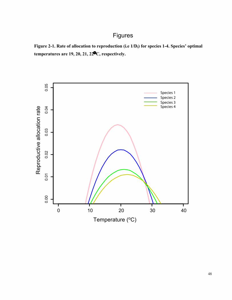
48
Figures
Figure 2-1. Rate of allocation to reproduction (i.e 1/Di) for species 1-4. Species’ optimal
temperatures are 19, 20, 21, 22°C, respectively.
! "! #! $! %!
!&!!
!&!"
!&!#
!&!$
!&!%
!&!'
()*+),-./,)01234
5)+,26/7.89)0-::27-.82;0,-.)
Species 1Species 2Species 3Species 4
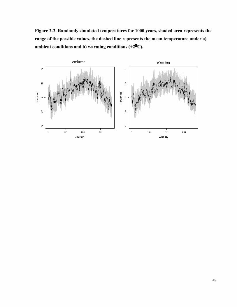
49
Figure 2-2. Randomly simulated temperatures for 1000 years, shaded area represents the
range of the possible values, the dashed line represents the mean temperature under a)
ambient conditions and b) warming conditions (+2°C).
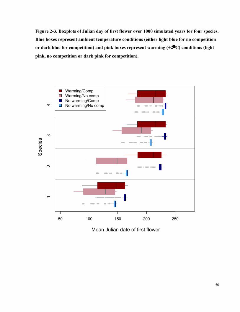
50
Figure 2-3. Boxplots of Julian day of first flower over 1000 simulated years for four species.
Blue boxes represent ambient temperature conditions (either light blue for no competition
or dark blue for competition) and pink boxes represent warming (+2°C) conditions (light
pink, no competition or dark pink for competition).
!" #"" #!" $"" $!"
%&'()*+,-'().'/&)01)1-23/)1,04&2
56&7-&3
12
34
8'29-(:;<0968'29-(:;=0)7096=0)4'29-(:;<096=0)4'29-(:;=0)7096
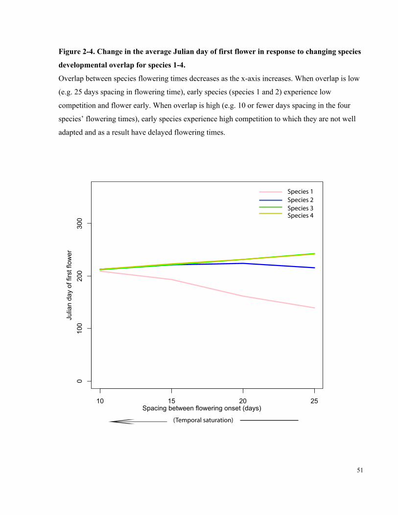
51
Figure 2-4. Change in the average Julian day of first flower in response to changing species
developmental overlap for species 1-4.
Overlap between species flowering times decreases as the x-axis increases. When overlap is low
(e.g. 25 days spacing in flowering time), early species (species 1 and 2) experience low
competition and flower early. When overlap is high (e.g. 10 or fewer days spacing in the four
species’ flowering times), early species experience high competition to which they are not well
adapted and as a result have delayed flowering times.
10 15 20 25
0100
200
300
Spacing between flowering onset (days)
Julian day of first flower
(Temporal saturation)
Species 1Species 2Species 3Species 4

52
Figure 2-5. Proportional distribution of flowering times Figure 3, for species 1-4, across all
combinations of warming and competition treatments.
Blue curves represent ambient temperature conditions (either light blue for no competition or
dark blue for competition) and pink curves represent warming (+2°C) conditions (light pink, no
competition or dark pink for competition).
! "!! #!! $!!
%&'()*+,-'().'/&)01)1-23/)1,04&2
56&7-&3
12
34
8'29-(:;<0968'29-(:;=0)7096=0)4'29-(:;<096=0)4'29-(:;=0)7096

53
Appendices
Appendix 2-1. Parameter values used for model simulations.
Parameter Value C 0/0.075 Tvar 4°C Popt 850 min Topt (19, 20, 21, 22°C) GTemp 17°C Db 1/(20, 40, 80, 100) p 5/(100, 80, 40, 20) ST 0.001 SP 0.0001 θ 1
Appendix 2-2. R code for model and simulations of warming in annual plant communities.
##Simulations library(zoo) library(geosphere) Photoperiod<-daylength(43.66,1:365) temp<-read.delim("Documents/Caroline/Evolution_warming/PhotoTemp2.txt") Temp<-temp[-366,] names(Temp)<-c("Temp","Julian") Temp<-cbind(Temp,Photoperiod) ##################################### species=4 season=nrow(Temp) P=Temp$Photoperiod*60 G<-rep(17,4) y=20
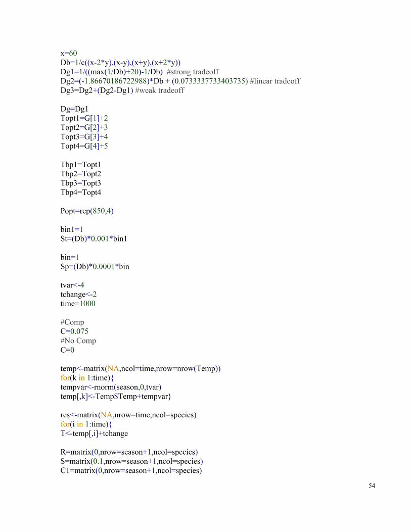
54
x=60 Db=1/c((x-2*y),(x-y),(x+y),(x+2*y)) Dg1=1/((max(1/Db)+20)-1/Db) #strong tradeoff Dg2=(-1.86670186722988)*Db + (0.0733337733403735) #linear tradeoff Dg3=Dg2+(Dg2-Dg1) #weak tradeoff Dg=Dg1 Topt1=G[1]+2 Topt2=G[2]+3 Topt3=G[3]+4 Topt4=G[4]+5 Tbp1=Topt1 Tbp2=Topt2 Tbp3=Topt3 Tbp4=Topt4 Popt=rep(850,4) bin1=1 St=(Db)*0.001*bin1 bin=1 Sp=(Db)*0.0001*bin tvar<-4 tchange<-2 time=1000 #Comp C=0.075 #No Comp C=0 temp<-matrix(NA,ncol=time,nrow=nrow(Temp)) for(k in 1:time){ tempvar<-rnorm(season,0,tvar) temp[,k]<-Temp$Temp+tempvar} res<-matrix(NA,nrow=time,ncol=species) for(i in 1:time){ T<-temp[,i]+tchange R=matrix(0,nrow=season+1,ncol=species) S=matrix(0.1,nrow=season+1,ncol=species) C1=matrix(0,nrow=season+1,ncol=species)
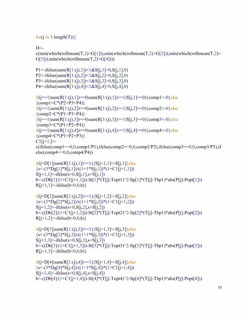
55
for(j in 1:length(T)){ D<-c(min(which(rollmean(T,2)>G[1])),min(which(rollmean(T,2)>G[2])),min(which(rollmean(T,2)>G[3])),min(which(rollmean(T,2)>G[4]))) P1<-ifelse(sum(R[1:(j),1])<1&S[j,1]>0,S[j,1],0) P2<-ifelse(sum(R[1:(j),2])<1&S[j,2]>0,S[j,2],0) P3<-ifelse(sum(R[1:(j),3])<1&S[j,3]>0,S[j,3],0) P4<-ifelse(sum(R[1:(j),4])<1&S[j,4]>0,S[j,4],0) if(j==1|sum(R[1:(j),1])==0|sum(R[1:(j),1])>=1|S[j,1]==0){comp1<-0}else {comp1=C*(P2+P3+P4)} if(j==1|sum(R[1:(j),2])==0|sum(R[1:(j),2])>=1|S[j,2]==0){comp2<-0}else {comp2=C*(P1+P3+P4)} if(j==1|sum(R[1:(j),3])==0|sum(R[1:(j),3])>=1|S[j,3]==0){comp3<-0}else {comp3=C*(P1+P2+P4)} if(j==1|sum(R[1:(j),4])==0|sum(R[1:(j),4])>=1|S[j,4]==0){comp4<-0}else {comp4=C*(P1+P2+P3)} C1[j+1,]<-c(ifelse(comp1==0,0,comp1/P1),ifelse(comp2==0,0,comp2/P2),ifelse(comp3==0,0,comp3/P3),ifelse(comp4==0,0,comp4/P4)) if(j<D[1]|sum(R[1:(j),1])>=1){S[j+1,1]<-S[j,1]}else {s<-(5*Dg[1]*S[j,1])/((1+1*S[j,1])*(1+C1[j+1,1])) S[j+1,1]<-ifelse(s<0,S[j,1],s+S[j,1]) b<-((Db[1]/(1+C1[j+1,1]))-St[1]*(T[j]-Topt1)^2-Sp[1]*(T[j]-Tbp1)*abs(P[j]-Popt[1])) R[j+1,1]<-ifelse(b<0,0,b)} if(j<D[2]|sum(R[1:(j),2])>=1){S[j+1,2]<-S[j,2]}else {s<-(5*Dg[2]*S[j,2])/((1+1*S[j,2])*(1+C1[j+1,2])) S[j+1,2]<-ifelse(s<0,S[j,2],s+S[j,2]) b<-((Db[2]/(1+C1[j+1,2]))-St[2]*(T[j]-Topt2)^2-Sp[2]*(T[j]-Tbp1)*abs(P[j]-Popt[2])) R[j+1,2]<-ifelse(b<0,0,b)} if(j<D[3]|sum(R[1:(j),3])>=1){S[j+1,3]<-S[j,3]}else {s<-(5*Dg[3]*S[j,3])/((1+1*S[j,3])*(1+C1[j+1,3])) S[j+1,3]<-ifelse(s<0,S[j,3],s+S[j,3]) b<-((Db[3]/(1+C1[j+1,3]))-St[3]*(T[j]-Topt3)^2-Sp[3]*(T[j]-Tbp1)*abs(P[j]-Popt[3])) R[j+1,3]<-ifelse(b<0,0,b)} if(j<D[4]|sum(R[1:(j),4])>=1){S[j+1,4]<-S[j,4]}else {s<-(5*Dg[4]*S[j,4])/((1+1*S[j,4])*(1+C1[j+1,4])) S[j+1,4]<-ifelse(s<0,S[j,4],s+S[j,4]) b<-((Db[4]/(1+C1[j+1,4]))-St[4]*(T[j]-Topt4)^2-Sp[4]*(T[j]-Tbp1)*abs(P[j]-Popt[4]))

56
R[j+1,4]<-ifelse(b<0,0,b)} } res[i,]<-c(ifelse(sum(R[,1])<1,0,which(cumsum(R[,1])==max(cumsum(R[,1])))[1]),ifelse(sum(R[,2])<1,0,which(cumsum(R[,2])==max(cumsum(R[,2])))[1]),ifelse(sum(R[,3])<1,0,which(cumsum(R[,3])==max(cumsum(R[,3])))[1]),ifelse(sum(R[,4])<1,0,which(cumsum(R[,4])==max(cumsum(R[,4])))[1])) }

57
Chapter 3 Fire variability, as well as frequency, can explain coexistence
between seeder and resprouter life histories
3 3
3.1 Abstract
Studies in fire-prone Mediterranean ecosystems have repeatedly shown that the mean values of
fire regimes (particularly frequency, but also size and intensity) are important for managing
sensitive species and maintaining diversity. However, recent studies suggest that invariant fire
regimes – i.e. those with no variation about the mean value—may not be sufficient to maintain
the coexistence mechanisms which could help explain the high levels of species diversity.
However, there has been little examination of the potential mechanisms by which variability in
fire regimes might foster coexistence.
In these species-diverse ecosystems, fluctuations in fire regimes promote the coexistence of
competitively unequal species, thus providing a potential mechanism of coexistence. We
examine the role of variability in the length of the inter-fire interval, and ask whether this
variability can allow a fluctuation-dependent mechanism, namely the storage effect, to promote
the coexistence of species. We focus on dominant trade-offs in fire regeneration strategies (i.e.
obligate resprouting versus obligate seeding) common among Mediterranean plant species and
use simulations to explore the interrelationship between variability in the time between fires and
the coexistence of species.
Several empirical studies have found that variability in the length of the inter-fire interval
improved diversity – our simulations suggested one mechanism that could explain this result.
Variability can greatly increase the regions over which coexistence between two species – a fire-
obligate seeder and a resprouter—occurs.
3.1.1 Synthesis and applications.
Mediterranean ecosystems tend to have high plant diversity, and yet the mechanisms maintaining
this diversity are often incompletely understood, and thus management actions that aim to

58
promote coexistence may be relying on imprecise information. In general though, fire events
drive the evolution and maintenance of diversity and are an important management tool. It is
highly likely that fluctuations or variability in fire are also important, and this suggests that
invariant regimes of prescribed burning or fire suppression could be detrimental to the
mechanisms that play a role in the maintenance of diversity in these Mediterranean ecosystems.
As a result, attention should be paid to historical fire regimes and the variation in fire return
times they displayed when developing prescribed burning regimes.
3.2 Introduction
Fire-dominated landscapes include some of the most diverse ecosystems on the planet, with the
fire-prone semi-arid shrublands in South Africa, California, Southwest Australia, and the
Mediterranean basin being recognized as globally important biodiversity hotspots, due to the
combination of high concentrations of endemic species and high habitat loss (Myers et al. 2000).
In some of these regions, fire regimes are actively managed to reduce fuel load and to control the
frequency and size of natural wildfires using prescribed burning (Wade & Lunsford 1989;
Fernandes & Botelho 2003). However, prescribed burning may also be applied to achieve
management goals that extend beyond hazard reduction to include ecosystem management goals
such as diversity maintenance (Bradstock et al. 1995; Richards et al. 1999; Haines et al. 2001).
However, the use of prescribed burning in ecosystem management is controversial (e.g. Morrison
et al. 1996; Clarke 2008; Reinhardt et al. 2008), and evidence suggests that fire management and
prescribed burns may not have the desired effects on community diversity and composition
compared to natural fire regimes (Bond & van Wilgen 1996). For example, attempts to protect
the rare fynbos shrub Orothamnus zeyheri by suppressing fires resulted in near extirpation of
populations, since the shrub was an obligate fire recruiter. Fortunately, controlled burns were
instituted before the species’ seed banks disappeared (Boucher 1981).
The different aspects of the fire regime – including fuel type, temporal nature and spatial pattern
(Bond & Keeley 2005) – affect diversity and coexistence, population size and persistence, the
likelihood of invasion, and ecosystem structure and services in Mediterranean-type and other
ecosystems (e.g. Boucher 1981; Richardson & van Wilgen 1992; Cary & Morrison 1995;
Bradstock & Kenny 2003; Brooks et al. 2004; Pausas et al. 2004; Bowman et al. 2009).

59
Determining targets related to fire frequency, intensity, or season, for managed fire regimes in
Mediterranean ecosystems (Gill 1975) is the focus of much research (for example, Gill 1977;
Gill & Bradstock 1997; Richards et al. 1999; McCarthy et al. 2001). This research focuses on the
length of the time between fires (the inter-fire interval) and its relationship to important life-
history events among plant species including maturation, seed bank accumulation, and
senescence. In the case of Mediterranean shrub species, when fires burn too frequently species
may not have time to mature and produce seed, leading to population extirpation (Gill & Groves
1981; Gill & Bradstock 1995; Pausas 2001). When fires occur too infrequently, seed banks of
species that require fire-related cues for germination may be lost (Pausas 2001), thereby limiting
population recruitment.
Variation in the inter-fire interval may also be important in determining the outcome of fire
regimes, but the effect of variation is much less understood (Cary & Morrison 1995; Bradstock et
al. 1996). Work from fire-prone heathlands in Australia suggests that invariant timing of fire
events can be harmful to overall diversity (Keith & Bradstock 1994; Morrison et al. 1995; but
see Wittkuhn et al. 2011), possibly because some mechanisms of coexistence rely on fluctuations
in fire occurrence. However, theoretical work explicitly considering the mechanisms that relate
variation in the fire interval and species diversity is still generally lacking, making it difficult to
determine how much variation should be incorporated into a fire regime to maintain diversity in
an ecosystem (Gill & McCarthy 1998).
The characteristics of present-day fire regimes in Mediterranean ecosystems are important
because species’ life histories are adaptations to historic fire regimes, the result of which is that
the timing and nature of fires determine species’ presences and abundances (Bond et al. 1990;
Bond & van Wilgen 1996; Bond & Midgley 2003; Bond & Keeley 2005). Across different
Mediterranean shrublands, convergent evolution has repeatedly produced woody, evergreen,
sclerophyllous shrub species (Mooney & Dunn 1970). Crown-fires in these shrublands consume
the majority of above-ground biomass, leading to a well-documented trade-off in post-fire
regeneration strategies among shrub species: species either rely on fire-stimulated germination or
post-fire resprouting behaviour (Mooney & Dunn 1970; Bond & Midgley 2003).

60
We hypothesize that variability in the length of the inter-fire interval may be one mechanism by
which fire promotes coexistence among species. In particular, we provide an example of a
possible mechanism – a temporal storage effect – through which variability in the length of the
inter-fire interval could promote species coexistence between an obligate resprouter and obligate
seeder. The storage effect (Chesson & Huntley 1997; Chesson 2000; Adler & Drake 2008) is a
form of temporal partitioning in which competing species show differential recruitment in
response to environmental conditions. There are several conditions required for the storage effect
to act (Chesson & Huntley 1997): 1) species must have differential responses to environmental
conditions including disturbances; 2) there must be covariance between competition and these
environmental conditions, which occurs when one species is favoured over another by particular
conditions; and 3) there must be a mechanism for buffered population growth, allowing species
to persist through unfavourable conditions when interspecific competition is high, by “storing”
fitness from past times when conditions were more favourable. Storage could be a result of long-
lived life history stages such as seed banks or long-lived perennials (Chesson 2000). Although
the focus is usually on fluctuations in the abiotic environment, variability in fire events can also
create a storage effect (e.g.Miller & Chesson 2009 ). Given that shrub species in Mediterranean
systems fulfil the requirements for the storage effect, we develop a model to show that varying
the length of the inter-fire interval could alter the effect of fire regimes on seeder and resprouter
species in Mediterranean ecosystems.
3.3 Materials and methods
3.3.1 Lottery model
We model the storage effect using a simple version of the lottery model (Chesson & Warner
1981). A lottery model considers the division of available sites among species as being in
proportion to their representation in the available pool of recruits (Sale 1977, 1978). Such a
model is useful for space-limited systems, where there are more recruits than there are available
sites for establishment, or to represent stochastic recruitment in systems where species appear
similar in form and function (Hubbell 2001). A simple formulation of the lottery model
represents the proportion of sites occupied by species i as:
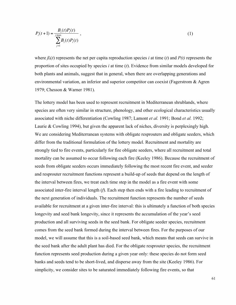
61
€
Pi(t +1) =Bi(t)Pi(t)
Bi(t)Pi(t)j=1
jmax
∑ , (1)
where ßi(t) represents the net per capita reproduction species i at time (t) and P(t) represents the
proportion of sites occupied by species i at time (t). Evidence from similar models developed for
both plants and animals, suggest that in general, when there are overlapping generations and
environmental variation, an inferior and superior competitor can coexist (Fagerstrom & Agren
1979; Chesson & Warner 1981).
The lottery model has been used to represent recruitment in Mediterranean shrublands, where
species are often very similar in structure, phenology, and other ecological characteristics usually
associated with niche differentiation (Cowling 1987; Lamont et al. 1991; Bond et al. 1992;
Laurie & Cowling 1994), but given the apparent lack of niches, diversity is perplexingly high.
We are considering Mediterranean systems with obligate resprouters and obligate seeders, which
differ from the traditional formulation of the lottery model. Recruitment and mortality are
strongly tied to fire events, particularly for fire obligate seeders, where all recruitment and total
mortality can be assumed to occur following each fire (Keeley 1986). Because the recruitment of
seeds from obligate seeders occurs immediately following the most recent fire event, and seeder
and resprouter recruitment functions represent a build-up of seeds that depend on the length of
the interval between fires, we treat each time step in the model as a fire event with some
associated inter-fire interval length (f). Each step then ends with a fire leading to recruitment of
the next generation of individuals. The recruitment function represents the number of seeds
available for recruitment at a given inter-fire interval: this is ultimately a function of both species
longevity and seed bank longevity, since it represents the accumulation of the year’s seed
production and all surviving seeds in the seed bank. For obligate seeder species, recruitment
comes from the seed bank formed during the interval between fires. For the purposes of our
model, we will assume that this is a soil-based seed bank, which means that seeds can survive in
the seed bank after the adult plant has died. For the obligate resprouter species, the recruitment
function represents seed production during a given year only: these species do not form seed
banks and seeds tend to be short-lived, and disperse away from the site (Keeley 1986). For
simplicity, we consider sites to be saturated immediately following fire events, so that

62
recruitment of both resprouting species (from seeds produced during the previous year) and
seeding species (from the seed bank accumulated over the time between fires) only occurs during
the post-fire period when mortality makes sites available. Here seeds in the seed bank are
considered to be in the soil and so survive past the death of the plant. As resprouters survive fire
events, we treat this as a situation when one species (resprouters) have overlapping generations,
while the other (seeders) does not.
This model shows the proportion of sites occupied by species i with adult population size Ni(f) at
a given fire (f):
€
Pi(t +1) = (1−δ i( f ))Pi( f ) + δ j ( f ))Pj ( f )j=1∑⎡
⎣ ⎢ ⎢
⎤
⎦ ⎥ ⎥
βi( f )Pi( f )( β j ( f )Pj ( f ))∑
⎡
⎣ ⎢ ⎢
⎤
⎦ ⎥ ⎥ , (2)
where ßi(f) represents the seed bank accumulated by species i over the current interval and P(f)
represents the proportion of sites occupied by species i at the end of the fire interval. Henceforth,
we will use the subscript Sp to represent the resprouter species, and the subscript Se to represent
the seeder species. δ represents mortality caused by a fire event: for the resprouter species this is
can take a range of values between 0 and 1, ranging from no, to total, mortality of adult
resprouters. This value can be a function of the inter-fire interval, or may be represented as a
constant value. For the seeder species, δ is set to 1, representing the total mortality of seeders
following a fire event.
For the seeder species, ßSe(f) represents the seed bank accumulated during the inter-fire period,
which we represent as a Gaussian function of the length of the inter-fire interval. The seeder
species is most common when fire intervals are intermediate, because recruitment is low when
fire intervals are too short to allow time for establishment and reproduction, or too long, causing
seed bank exhaustion (Keeley 1986; Bond & van Wilgen 1996; Schwilk et al. 1997; Pausas
2001).
€
βSe ( f ) = c⋅ e−( f −µ )2
2σ 2 , (3)
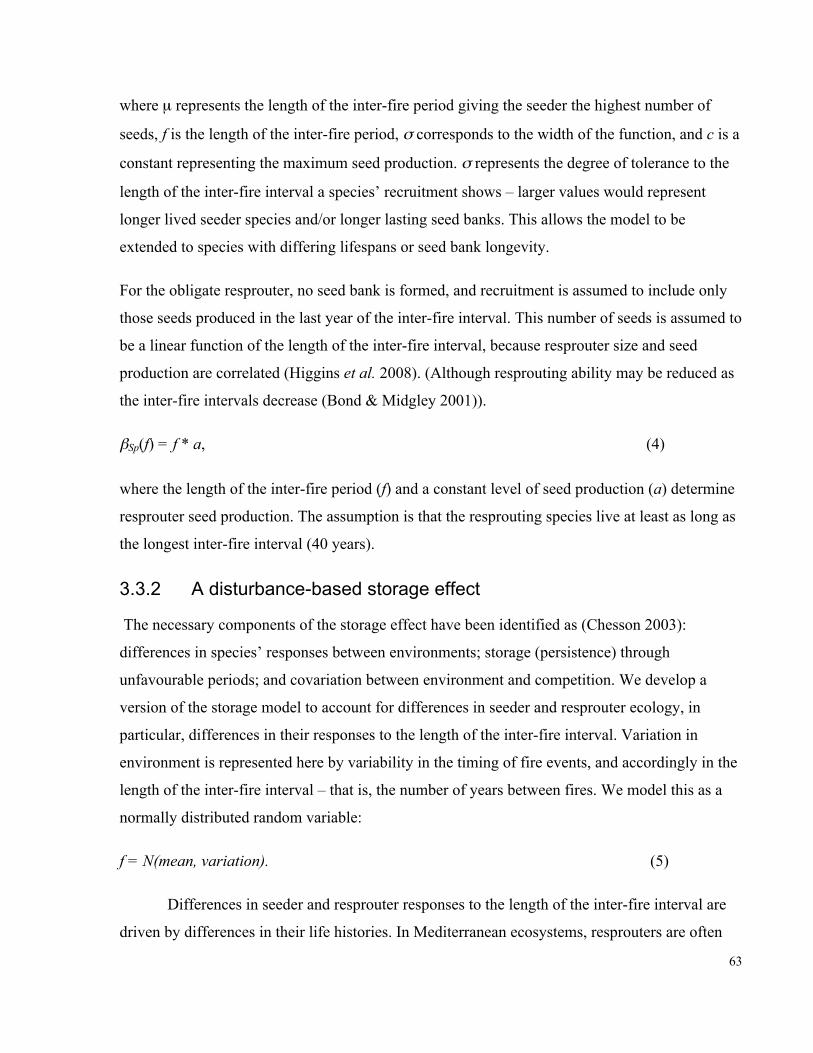
63
where µ represents the length of the inter-fire period giving the seeder the highest number of
seeds, f is the length of the inter-fire period, σ corresponds to the width of the function, and c is a
constant representing the maximum seed production. σ represents the degree of tolerance to the
length of the inter-fire interval a species’ recruitment shows – larger values would represent
longer lived seeder species and/or longer lasting seed banks. This allows the model to be
extended to species with differing lifespans or seed bank longevity.
For the obligate resprouter, no seed bank is formed, and recruitment is assumed to include only
those seeds produced in the last year of the inter-fire interval. This number of seeds is assumed to
be a linear function of the length of the inter-fire interval, because resprouter size and seed
production are correlated (Higgins et al. 2008). (Although resprouting ability may be reduced as
the inter-fire intervals decrease (Bond & Midgley 2001)).
βSp(f) = f * a, (4)
where the length of the inter-fire period (f) and a constant level of seed production (a) determine
resprouter seed production. The assumption is that the resprouting species live at least as long as
the longest inter-fire interval (40 years).
3.3.2 A disturbance-based storage effect
The necessary components of the storage effect have been identified as (Chesson 2003):
differences in species’ responses between environments; storage (persistence) through
unfavourable periods; and covariation between environment and competition. We develop a
version of the storage model to account for differences in seeder and resprouter ecology, in
particular, differences in their responses to the length of the inter-fire interval. Variation in
environment is represented here by variability in the timing of fire events, and accordingly in the
length of the inter-fire interval – that is, the number of years between fires. We model this as a
normally distributed random variable:
f = N(mean, variation). (5)
Differences in seeder and resprouter responses to the length of the inter-fire interval are
driven by differences in their life histories. In Mediterranean ecosystems, resprouters are often

64
observed to have lower seed recruitment than seeder species, and being outcompeted by seeders
(Keeley 1986; Burgman & Lamont 1992; Pausas 2001). While there is variation among
Mediterranean ecosystems in seeder and resprouter life histories and in fire regimes, we follow a
general model where seeders dominate at intermediate inter-fire intervals and resprouter at low
and high inter-fire intervals (Burgman & Lamont 1992; Pausas 2001).
Finally, both the seeder and resprouter species can buffer their fitness, either through fire
tolerance and survival of resprouters, or seed bank formation by seeders. Competition among
seeder and resprouter species occurs primarily during the recruitment of seedlings (Yeaton &
Bond 1991; Laurie & Cowling 1994), and once established, adult resprouters may persist for
multiple fire cycles. Hence resprouters that establish during favourable periods can maintain their
populations by persisting through unfavourable periods. Seeds produced by seeder species are
either stored in serotinous seed banks or, particularly in the South Africa and Australia, cached
underground by ants. Comprehensive data on the longevity of these buried seeds is lacking, but
at least some buried seeds from seeder species may remain viable for longer periods of time and
this confers some buffering of fitness (Holmes & Cowling 1997; Auld et al. 2000; Holmes &
Newton 2004; Willis & Read 2007). As stated earlier, we assume soil-based seed banks in this
analysis.
For simplicity’s sake, we model a generic obligate resprouter and obligate seeder species with a
soil-based seed bank in an ecosystem with similar fire regimes as those found in the Cape
Floristic Region of South Africa (CapeNature & SANBI 2008). Although this is necessarily a
simplification of the actual relationship between seeders and resprouters and fire (and it ignores
species-specific differences), it is sufficient to highlight how fluctuations in fire occurrences
could promote long-term persistence of these life histories.
3.3.3 Numerical simulations
We chose to simulate a co-occurring obligate seeder and obligate resprouter species in a
system where the mean length of the inter-fire interval ranged between 0–40 years and varied by
between 0–15 years (see Appendix 3-1 in Supporting Information for R code). This represents a
realistic range of values for the Cape Floristic Region of South Africa (CapeNature & SANBI
2008), but the specific values are less important than the necessity that the requirements of the
65
storage effect be met, and any Mediterranean ecosystem could have been modelled provided the
life histories of species and their relationship to historical fire regimes were understood. The total
number of available sites in a community was set to 1000, and initial starting populations were
set in accordance to invasion analysis: i.e. the invading species had a starting population of 1
individual, and the resident a starting population of 999. The invader was considered the species
with the fewer seeds available for recruitment for each length of the inter-fire interval, when
variability in length of the inter-fire interval is zero, given the parameter values used for a and c
(see below).
We repeated the simulations 1000 times at each combination of inter-fire interval (for lengths
between 0 and 40 years) and variation (from 0 to 15 years), a total of 600,000 simulations. It
should be noted that regimes with short periods between fires and high variability are unlikely to
be observed in nature. For each simulation, we recorded the proportion of the community
occupied by resprouters and seeders after 1000 time steps. We calculated the probability of
coexistence at each combination of inter-fire length and variability as the number of runs per
1000 in which seeders and resprouters persisted together after 1000 time steps. Persistence was
defined as occupying at least 1 site in the community after the 1000 time steps. Throughout the
results, where we refer to “coexistence” we imply this definition of long-term persistence, rather
than analytical coexistence.
3.3.4 Parameter value selection
The numbers of seeds available for recruitment at time each fire event were set to c = 8000
(Equation 3) for seeders and a = 50 (Equation 4) for resprouters. c is equivalent to the
accumulated seed bank available for recruitment for seeders; this seed bank is modelled to be
largest when the fire-return interval (µ) is 20 years (Figure 3-1), which is equivalent to saying
that the combination of seeder life span and seed bank longevity result in the greatest number of
seeds at 20 years. We examine the effects of changing the seeder seed recruitment function, to
account for different species lifespans or seed bank longevity: however, the results of our
simulation do not fundamentally change (Figure S1). Resprouters are likely to have far fewer
seeds available for recruitment (Bond & Midgley 2001) (one record from the CFR found that
resprouters produced between 9.7% to 88.0% of the number of cones produced by seeder
66
species (Higgins et al. 2008)), and resprouters do not form a lasting seed bank (Keeley 1986).
Given these parameter values, resprouters are invaders for sites with fire frequencies less than
~33 years. Resprouters were invaders for sites with frequencies between those values. Resprouter
fire mortality (δSp) was set to 0.25 (i.e. 75% survival). We examine the sensitivity of our model
to the difference in the number of seeds available for recruitment between seeders and
resprouters (see below).
3.3.5 Sensitivity of the model to parameter values
One essential question is how important is the difference in the seeds available for recruitment
for seeders and resprouters. We examined how altering the number of seeder and resprouter
seeds available changed the likelihood of coexistence at different inter-fire intervals. We expect
that there should be a relationship between the amount of variation that allows coexistence, the
differences in seeds available for recruitment, and the amount of storage that the species have
(Chesson 2000). To explore this relationship, we simulated all combinations of parameters of
length of inter-fire period variation (f ∈ [0,40]), buffering (δSp ∈ [0.1,0.9]), and the difference in
the number of seeds available for recruitment between seeder and resprouter (c ∈ [3000,10000],
a ∈ [10,300]) and recorded the corresponding minimum variation in length of inter-fire period
required for coexistence at each combination of these.
An important point is that the storage effect should not function in the absence of some form of
storage or buffering that allows species to maintain their populations through unfavourably short
or long inter-fire intervals. For example, if the resprouter species are no longer able to survive
fire events, variability in the length of the inter-fire period should not promote coexistence of the
seeder and resprouter species. We removed buffering of resprouter fitness by setting δSp to 0, so
that no adult resprouters survive fire events. We then repeated the simulations 1000 times at each
combination of length of inter-fire period (for fire frequencies between 0 and 40 years) and
variation (for values ranging from 0 to 15 years). For each simulation, we recorded the
proportion of the community occupied by resprouters and seeders after 1000 time steps.

67
3.4 Results
3.4.1 Coexistence with non-variable fire return:
When there is no variability in the length of the interval between fires, there is a small range of
fire frequencies where the seeder and resprouter species are expected persist (Figure 3-2A,
greyed regions 2, 4). These regions reflect the length of the inter-fire period that minimize the
difference in recruitment between seeders and resprouters and allow persistence under the lottery
model. However, for the majority of fire frequencies only one of the two species is predicted to
persist when variability is set to 0 (Figure 3-2B, regions 1, 3, 5).
3.4.2 Coexistence with variable fire return
When variability in the length of the inter-fire period is incorporated, persistence of seeders and
resprouters can occur in regions where exclusion occurred in the absence of variation (Figure 3-
2B, 1–5). For example, in region 3 (Figure 3-2B–3) where the seeder species excluded the
resprouter species when variability is zero, increased variation means that the resprouter species
periodically has high recruitment, which, combined with buffered population growth, allows its
population to coexist with the seeder species. In contrast, higher variability can decrease the
ability of the seeder to persist (region 4), by increasing the number of unfavourably long inter-
fire intervals. Ultimately, the likelihood that the seeder and resprouter species coexist is
determined by the interaction between the length of the inter-fire interval (and implicitly, its
relationship with the number of seeder and resprouter seeds available for recruitment) and the
variability in this length, which interacts with buffering ability (Figure 3-3). When variation in
the length of inter-fire period is 0 in this plot, the red regions of coexistence are equivalent to the
grey areas in Figure 3-2a. There is a high probability of coexistence of the seeder and resprouter
species across the widest range of fire frequencies when the variability is ~8.5 years. In fact,
when variation is this high, the resprouter and seeder species coexist across nearly all inter-fire
intervals below 30 years.
When adult mortality of the resprouter species was set to 1, so that there was no storage of fitness
between generations for that species, variability in length of inter-fire period did not increase the
region over which resprouters and seeders could coexist (Figure 3-4).

68
3.4.3 Influence of parameter values on coexistence
The values of a and c that we chose appear to be less important to the outcome of our model than
the overall difference in the number of seeds available for recruitment between seeders and
sprouters. Figure 3-5 suggests that there is a relationship between the size of this difference in
seed number and the mortality resprouters experience during fire events, and the corresponding
amount of variation necessary for coexistence. When seeders have more seeds available for
recruitment, greater variability in the inter-fire interval is necessary for the resprouters to coexist.
When resprouter mortality is low, resprouters are able to maintain sites and more effectively
compete, so less variability is required for their coexistence with seeders. When resprouter
mortality is higher, greater variability is required for coexistence. The initial choice of parameter
values (a and c) for the resprouter and seeder species is not as important as having the essential
components of the storage effect present, i.e. variation in length of inter-fire period and buffering
of fitness.
3.5 Discussion
We found that variability in the length of time between fires can greatly increase the likelihood
of coexistence between species with obligate seeder and obligate resprouter life histories. This
trade-off (between seeder and resprouter life histories) is common in Mediterranean ecosystems.
In many ecosystems, recurrent fires are necessary to maintain community composition and
diversity (Cowling & Campbell 1980; Keeley 1986), in part because disturbance creates
opportunities for temporal niche differentiation (Bonis et al. 1995; Buckling et al. 2000). In such
situations, invariant fire return intervals would be likely to reduce diversity by removing
temporal niches for differentiation among species. However, achieving a balance between risk
reduction through fire management and diversity maintenance may be difficult, especially when
it is unclear which aspects of natural fire regimes must be retained for diversity maintenance. For
example, maintaining an appropriate mean return interval between fires but neglecting variability
in the return interval could lead to a reduction in diversity, if coexistence depends on temporal
fluctuations in fire events.
Historically, fires regimes were both spatially and temporally variable. Fire regimes in
Mediterranean ecosystems were initiated by lightning strikes (prior to human habitation) and
69
initiation was probabilistic, dependent on the combination of suitable weather and fuel conditions
in addition to the initial spark (Keeley et al. 1989; Keeley & Fotheringham 2003). In fact, most
aspects of fires were likely much more variable in the past (Keeley et al. 2005). Plant species in
Mediterranean ecosystems show clear adaptations that allow post-fire regeneration (seed banks,
resprouting ability), and can provide a buffering mechanism against some variability in fire
return intervals. It may be that managed fire regimes should account for the historical variability
in fire return in a region and the life history traits of species present that have evolved in
response to it. Although there have been few empirical studies looking at the relationship
between variability in the length of the inter-fire interval and diversity, Morrison et al. (1995)
found that variability in the length of the inter-fire interval is associated with increased diversity
of both fire sensitive and fire tolerant species, similar to the expectation of a storage effect.
Although we did not explore the effect of variability over multiple spatial scales, both temporal
variability and spatial variability in the length of the inter-fire period could be important in these
regions. The combination of both temporal rescue of populations via storage, and spatial rescue
via seed dispersal could concurrently act to maintain diversity in fire prone ecosystems (Miller &
Chesson 2009). While our results show that the coexistence of resprouter and seeder species may
even be possible in the absence of variability, in situations with multiple (>2) species, variability
may be an important coexistence mechanism.
The exact shape of the relationship between resprouter and seeder seed recruitment, and the
length of fire return interval in different Mediterranean regions will differ from our model
(Bellingham & Sparrow 2004), since different fire regimes have different selective effects on the
relationship between seeder or resprouter fitness and the fire return interval (for example, in the
Californian chaparral some obligate seeders may reestablish even after 100+ years between fires
(Keeley 1986)). However, the seed recruitment curves implicitly encompass a number of life
history traits, including seed bank longevity and species lifespan, making them flexible across
different species and ecosystems where these traits may vary in complex ways. Our model is also
flexible in terms of parameter values (degree of buffering, shape of the relationship between
seeder and resprouter fitness and fire), and only requires that the components of the storage
effect be present. It is of particular importance that buffering must be present, since systems
where species show little ability to tolerate unfavourable conditions will do poorly when

70
variation is increased. Further, the storage effect, modelled here to explain a two-species
interaction, could explain the coexistence of multiple seeder and resprouter species, if these
species are differentiated along additional axes relating to fire conditions (intensity) and/or
specialized within the seeder or resprouter response, or even partitioned along other aspects of
the biotic and abiotic environment.
3.5.1 Management implications
For high-diversity Mediterranean regions, the specific mechanisms by which disturbance can
contribute to and promote coexistence have important management implications. In most fire-
prone systems, species have evolved to historical fire regimes and it is highly probable that
historical fire regimes were variable. In these systems, even if there is an absence of species-
specific information about fire responses, it should be assumed that fire is an important aspect of
species coexistence. In these cases, we argue, management programs need to consider the
variability, as well as frequency, in fire events. The storage effect may be a fundamentally
important coexistence mechanism in these systems, and management activities that remove
variability in fire occurrence could ultimately result in population declines and extinctions. Thus
it is increasingly important to develop mechanistic models of the relationship between diversity
maintenance and fire in these species-rich, fire-prone systems. However, the value of variability
in managed fire regimes must be balanced against the higher fuel loads that result from longer
than average inter-fire intervals, and the increased risk of large, high-intensity fires which put
human communities and property at risk. It will remain important to optimize risk management
against the ecological gains of incorporating variability into fire regimes in Mediterranean
ecosystems.
71
References
Adler, P.B. & Drake, J.A. (2008) Environmenatl variation, stochastic extinction, and competitive coexistence. The American Naturalist, 172(5).
Auld, T.D., Keith, D.A. & Bradstock, R.A. (2000) Patterns in logevity of soil seedbanks in fire-prone communities of south-eastern Australia. Australian Journal of Botany, 48, 539-548.
Bellingham, P.J. & Sparrow, A.D. (2004) Resprouting as a life history strategy in woody plant communities. Oikos, 89, 409-416.
Bond, W.J., Cowling, R.M. & Richards, M.B. (1992) Competition and coexistence in proteoid shrubs. The ecology of fynbos: fire, nutrients, and diversity (ed. R.M. Cowling), pp. 206-225. Oxford University Press, Cape Town.
Bond, W.J. & Keeley, J.E. (2005) Fire as a global 'herbivore': the ecology and evolution of flammable ecosystems. Trends in Ecology and Evolution, 20, 387-394.
Bond, W.J., LeRoux, D. & Erntzen, R. (1990) Fire intensity and regeneration of myrmecochorous Proteaceae. South African Journal of Botany, 56, 326-330.
Bond, W.J. & Midgley, G.F. (2001) Ecology of sprouting woody plants: the persistence niche. Trends in Ecology and Evolution, 16, 45-51.
Bond, W.J. & Midgley, J.J. (2003) The evolutionary ecology of sprouting in woody plants. International Journal of Plant Sciences, 164, S103-S114.
Bond, W.J. & van Wilgen, B.W. (1996) Fire and Plants. Chapman & Hall, London.
Bonis, A., Lepart, J. & Grillas, P. (1995) Seed bank dynamics and coexistence of annual macrophytes in a temporary and variable habitat. Oikos, 74, 81-92.
Boucher, C. (1981) Autoecological and population studies of Orothamnus zeyheri in the Cape of South Africa. The Biological Aspects of Rare Plant Conservation (ed. H. Synge), pp. 343-353. Chichester etc., Wiley, Cambridge, UK.
Bowman, M.J.S., Balch, J.K., Artaxo, P., Bond, W.J., Carlson, J.M., Cochrane, M.A., D'Antonio, C.M., DeFries, R.S., Doyle, J.C., Harrison, S.P., Johnston, F.H., Keeley, J.E., Krawchuk, M.A., Kull, C.A., Marston, J.B., Moritz, M.A., Prentice, I.C., Roos, C.I., Scott, A.C., Swetnam, T.W., van der Werf, G.R. & Pyne, S.J. (2009) Fire in the earth system. Science, 324, 481-484.
Bradstock, R.A., Bedward, M., Scott, J. & Keith, D.A. (1996) Simulation of the effect of spatial and temporal variation in fire regimes on the population viability of a Banksia species. Conservation Biology, 10, 776-784.
Bradstock, R.A., Keith, D.A. & Auld, T.D. (1995) Fire and conservation: imperatives and constraints on managing diversity. Conserving biodiversity: Threats and Solutions (eds R.A. Bradstock, T.D. Auld, D.A. Keith, R.T. Kingsford, D. Lunney & D.P. Sivertsen).
Bradstock, R.A. & Kenny, B.J. (2003) Application of plant functional types to fire management. Journal of Vegetation Science, 14, 345-354.

72
Brooks, M.L., D'Antonio, C.M., Richardson, D.M., Grace, J.B., Keeley, J.E., DiTomaso, J.M., Hobbs, R.J., Pellant, M. & Pyke, D. (2004) Effects of Invasive Alien Plants on Fire Regimes. Bioscience, 54, 677-688.
Buckling, A., Kassen, R., Bell, G. & Rainey, P.B. (2000) Disturbance and diversity in experimental microcosms. Nature, 408, 961-964.
Burgman, M.A. & Lamont, B.B. (1992) A stochastic model for the viability of Banksi cuneata populations: environmental, demographic and genetic effects. Journal of Applied Ecology, 29, 719-727.
CapeNature & SANBI (2008) GIS Metadata - all_fires_07_08.shp. (ed. C. Tucker). Cape Town.
Cary, G.J. & Morrison, D.A. (1995) Effects of fire frequency on plant species composition of sandstone communities in the Sydney region: Combinations of inter-fire intervals. Australian Journal of Ecology, 20, 418-426.
Chesson, P. (2000) Mechanisms of maintenance of species diversity. Annual Review of Ecology and Systematics, 31, 343-366.
Chesson, P. (2003) Quantifying and testing coexistence mechanisms arising from recruitment fluctuations. Theoretical Population Biology, 4, 345-357.
Chesson, P. & Huntley, N. (1997) The roles of harsh and fluctuating conditions in the dynamics of ecological communities. The American Naturalist, 150, 519-553.
Chesson, P. & Warner, R.R. (1981) Environmental variability promotes coexistence in lottery competitive systems. American Naturalist, 117, 923-943.
Clarke, M.F. (2008) Catering for the needs of fauna in fire management: science or just wishful thinking? Wildlife Research, 35, 385-394.
Cowling, R.M. (1987) Fire and its role in coexistence and speciation in Gondwanan shrublands. South African Journal of Science, 83, 106-112.
Cowling, R.M. & Campbell, B.M. (1980) Convergence in the vegetation structure in the Mediterranean communities of California, Chile, and South Africa. Plant Ecology, 43, 191-197.
Fagerstrom, T. & Agren, G.I. (1979) Theory for coexistence of species differing in regeneration properties. Oikos, 33, 1-10.
Fernandes, P.M. & Botelho, H.S. (2003) A review of prescribed burning effectiveness in fire hazard reduction. International Journal of Wildland Fire, 12, 117-128.
Gill, A.M. (1975) Fire and the Australian flora: a review. Australian Forestry, 38, 4-28.
Gill, A.M. (1977) Management of fire-prone vegetation for plant species conservation in Australia. Journal of the Australian and New Zealand Association for the Advancement of Science, 8, 20-26.
Gill, A.M. & Bradstock, R.A. (1995) Extinction of biota by fires. Conserving biodiversity: Threats and Solutions (eds R.A. Bradstock, T.D. Auld, D.A. Keith, R.T. Kingsford, D. Lunney & D.P. Sivertson), pp. 309-322. Surrey Beatty and Sons, Sydney, Australia.
73
Gill, A.M. & Bradstock, R.A. (1997) Prescribed burning: patterns and strategies. 13th International Conference on Fire and Forest Meteorology. Victoria, Australia.
Gill, A.M. & Groves, R.H. (1981) Fire regimes in heathlands and their plant-ecological effects. Ecosystems of the world, 9B, Heathlands and Related Shrublands (ed. R.L. Specht), pp. 61-84. Elsevier, Amsterdam.
Gill, A.M. & McCarthy, M.A. (1998) Intervals between prescribed fires in Australia: what intrinsic variation should apply? Biological conservation, 85, 161-169.
Haines, T.K., Busby, R.L. & Cleaves, D.A. (2001) Prescribed burning in the South: trends, purpose, and barriers. Southern Journal of Applied Forestry, 25, 149-153.
Higgins, S.I., Flores, O. & Schurr, F.M. (2008) Costs of persistence and the spread of competing seeders and sprouters. Journal of Ecology, 96, 679-686.
Holmes, P.M. & Cowling, R.M. (1997) Diversity, composition and guild structure relationships between soil-stored seed banks and mature vegetation in alien plant-invaded South African fynbos shrublands. Plant Ecology, 133, 107-122.
Holmes, P.M. & Newton, R.J. (2004) Patterns of seed persistence in South African Fynbos. Plant Ecology, 172, 143-158.
Hubbell, S.P. (2001) The Unified Neutral Theory of Biodiversity and Biogeography. Princeton University Press. Princeton, NJ.
Keeley, J.E. (1986) Resilience of Mediterranean shrub communities to fire. Resilience in Mediterranean-type Ecosystems (eds B. Dell, A.J.M. Hopkins & B.B. Lamont). Dr. W. Junk Publishers, Dordrecht.
Keeley, J.E. & Fotheringham, C.J. (2003) Impact of past, present, and future fire regimes on North American Mediterranean shrublands. Ecological studies, 160, 218-262.
Keeley, J.E., Fotheringham, C.J. & Baer-Keeley, M. (2005) Factors affecting plant diversity during post-fire recovery and succession of Mediterranean-climate shrublands in California, USA. Diversity and Distributions, 11, 525-537.
Keeley, J.E., Zedler, P.H., Zammit, C.A. & Stohlgren, T.J. (1989) Fire and demography. The California Chaparral. Paradigms reexamined. (ed. N.H.M.o.L.A. County). Los Angeles.
Keith, D.A. & Bradstock, R.A. (1994) Fire and competition in Australian heath: a conceptual model and field investigation. Journal of Vegetation Science, 5, 347-354.
Lamont, B.B., Connell, S.W. & Bergl, S.M. (1991) Seed bank and population dynamics of Banksia cuneata: the role of time, fire, and moisture. Botanical Gazette, 152, 114-122.
Laurie, H. & Cowling, R.M. (1994) Lottery coexistence models exteded to plants with disjoint generations. Journal of Vegetation Science, 5, 161-168.
McCarthy, M.A., Possingham, H.P. & Gill, A.M. (2001) Using stochastic dynamic programming to determine optimal fire management for Banksia ornata. Journal of Applied Ecology, 38.
74
Miller, A.D. & Chesson, P. (2009) Coexistence in disturbance-prone communities: how a resistance-resilience trade-off generates coexistence via the storage effect. The American Naturalist, 173, E30-E43.
Mooney, H.A. & Dunn, E.L. (1970) Convergent Evolution of Mediterranean-Climate Evergreen Sclerophyll Shrubs. Evolution, 24, 292-303.
Morrison, D.A., Buckney, R.T., Bewick, B.J. & Cary, G.J. (1996) Conservation conflicts over burning bush in south-eastern Australia. Biological conservation, 76, 175.
Morrison, D.A., Cary, G.J., Pengelly, S.M., Ross, D.G., Mullins, B.J., Thomas, C.R. & Anderson, T.S. (1995) Effects of fire frequency on plant species composition of sandstone communities in the Sydney region: inter-fire interval and time-since-fire. Australian Journal of Ecology, 20, 239-247.
Myers, N., Mittermeier, R.A., Mittermeier, C.G., da Fonseca, G.A.B. & Kent, J. (2000) Biodiversity hotspots for conservation priorities. Nature, 403, 853-858.
Pausas, J.G. (2001) Resprouting vs seeding: A Mediterranean perspective. Oikos, 94, 193-194.
Pausas, J.G., Bradstock, R.A., Keith, D.A. & Keeley, E.R. (2004) Plant functional traits in relation to fire in crown-fire ecosystems. Ecology, 85, 1085-1100.
Reinhardt, E.D., Keane, R.E., Calkin, D.E. & Cohen, J.D. (2008) Objectives and considerations for wildland fuel treatment in forested ecosystems of the interior western United States. United States Forest Ecology and Management, 256, 1997-2006.
Richards, S.A., Possingham, H.P. & Tizard, J. (1999) Optimal fire management for maintaining community diversity. Ecological Applications, 9, 880-892.
Richardson, D.M. & van Wilgen, B.W. (1992) Ecosystem, community and species response to fire in mountain fynbos: conclusions from the Swartboskloof experiment. Ecological studies: analysis and synthesis, 93, 273-284.
Sale, P.F. (1977) Maintenance of high diversity in coral reef communities. The American Naturalist, 111, 337-359.
Sale, P.F. (1978) Coexistence of coral reef fishes--a lottery for living space. Environmental Biology of Fishes, 3, 85-102.
Schwilk, D.W., Keeley, J.E. & Bond, W.J. (1997) The intermediate disturbance hypothesis does not explain fire and diversity pattern in fynbos. Plant Ecology, 132, 77-84.
Wade, D. & Lunsford, J.D. (1989) A Guide for Prescribed Fire in Southern Forests. (ed. U.F. Service). Atlanta, GA.
Willis, T.J. & Read, J. (2007) Soil seed bank dynamics in post-fire heathland succession in south-eastern Australia. Plant Ecology, 190.
Wittkuhn, R.S., McCaw, L., Wills, A.J., Robinson, R., Anderson, A.N., Van Heurck, P., Farr, J., Liddelow, G. & Cranfield, R. (2011) Variation in fire interval sequences has minimal effects on species richenss and composition in fire-prone landscapes of south-west Western Australia. Forest Ecology and Management, 261, 965-978.

75
Yeaton, R.I. & Bond, W.J. (1991) Competition between two shrub species: dispersal differences and fire promote coexistence. The American Naturalist, 138, 328-341.

76
Figures
Figure 3-1. Conceptual model showing the number of seeds available for recruitment (β i,
Equation 2) as a function of the length of the inter-fire interval (f) for a generic seeder (red)
and resprouter (black) species. c=8000 and a=50. See Materials and methods for further
details on parameterization.
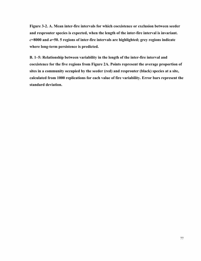
77
Figure 3-2. A. Mean inter-fire intervals for which coexistence or exclusion between seeder
and resprouter species is expected, when the length of the inter-fire interval is invariant.
c=8000 and a=50. 5 regions of inter-fire intervals are highlighted; grey regions indicate
where long-term persistence is predicted.
B. 1–5: Relationship between variability in the length of the inter-fire interval and
coexistence for the five regions from Figure 2A. Points represent the average proportion of
sites in a community occupied by the seeder (red) and resprouter (black) species at a site,
calculated from 1000 replications for each value of fire variability. Error bars represent the
standard deviation.
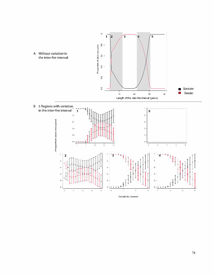
78
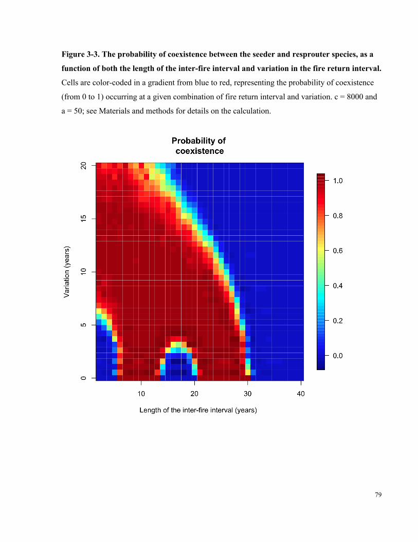
79
Figure 3-3. The probability of coexistence between the seeder and resprouter species, as a
function of both the length of the inter-fire interval and variation in the fire return interval.
Cells are color-coded in a gradient from blue to red, representing the probability of coexistence
(from 0 to 1) occurring at a given combination of fire return interval and variation. c = 8000 and
a = 50; see Materials and methods for details on the calculation.
80
Figure 3-4. The probability of coexistence between seeders and resprouters when there is
no storage for the resprouter species (i.e. δ = 1), as a function of the length of the inter-fire
interval and variation in the length of the inter-fire interval.
Cells are color-coded in a gradient from blue to red, representing the probability of coexistence
(from 0 to 1) occurring at a given combination of fire return interval and variation.
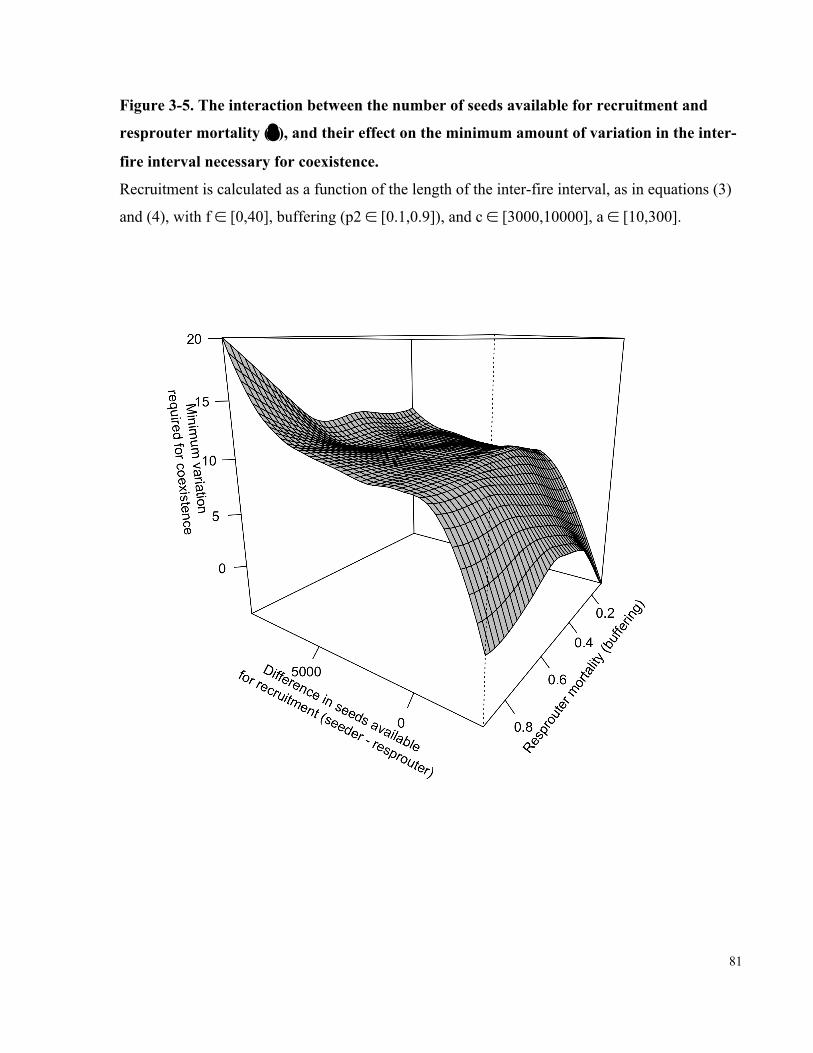
81
Figure 3-5. The interaction between the number of seeds available for recruitment and
resprouter mortality (δ), and their effect on the minimum amount of variation in the inter-
fire interval necessary for coexistence.
Recruitment is calculated as a function of the length of the inter-fire interval, as in equations (3)
and (4), with f ∈ [0,40], buffering (p2 ∈ [0.1,0.9]), and c ∈ [3000,10000], a ∈ [10,300].
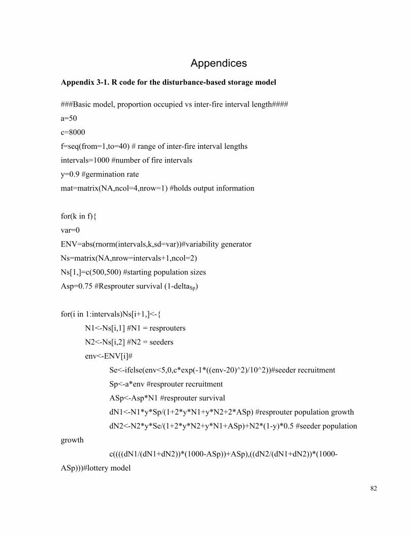
82
Appendices
Appendix 3-1. R code for the disturbance-based storage model
###Basic model, proportion occupied vs inter-fire interval length####
a=50
c=8000
f=seq(from=1,to=40) # range of inter-fire interval lengths
intervals=1000 #number of fire intervals
y=0.9 #germination rate
mat=matrix(NA,ncol=4,nrow=1) #holds output information
for(k in f){
var=0
ENV=abs(rnorm(intervals,k,sd=var))#variability generator
Ns=matrix(NA,nrow=intervals+1,ncol=2)
Ns[1,]=c(500,500) #starting population sizes
Asp=0.75 #Resprouter survival (1-deltaSp)
for(i in 1:intervals)Ns[i+1,]<-{
N1<-Ns[i,1] #N1 = resprouters
N2<-Ns[i,2] #N2 = seeders
env<-ENV[i]#
Se<-ifelse(env<5,0,c*exp(-1*((env-20)^2)/10^2))#seeder recruitment
Sp<-a*env #resprouter recruitment
ASp<-Asp*N1 #resprouter survival
dN1<-N1*y*Sp/(1+2*y*N1+y*N2+2*ASp) #resprouter population growth
dN2<-N2*y*Se/(1+2*y*N2+y*N1+ASp)+N2*(1-y)*0.5 #seeder population
growth
c((((dN1/(dN1+dN2))*(1000-ASp))+ASp),((dN2/(dN1+dN2))*(1000-
ASp)))#lottery model

83
}
mat<-rbind(mat,c(k,var,Ns[1000,]))
}
tot<-mat[-1,]
plot(tot[-1,3]/1000~tot[-1,1],type="l",xlab="Length inter-fire interval (years)",ylab="Proportion
of sites occupied",ylim=c(0,1))
points(tot[-1,4]/1000~tot[-1,1],type="l",col="red",lty="dashed",ylim=c(0,1))
legend(y=0.900,x=30,c("Resprouter","Seeder"),fill=c("black","red"))

84
Copyright Acknowledgements
Tucker, C.M. and Cadotte, M.W. 2013. Fire variability, as well as frequency, can explain
coexistence between seeder and resprouter life histories. Journal of Applied Ecology. DOI:
10.1111/1365-2664.12073.
Copyright © 2000-2008 by John Wiley & Sons, Inc. or related companies. All rights reserved.

85
Chapter 4 Incorporating geographical and evolutionary rarity into
conservation prioritization
4 4
4.1 Abstract
Key goals of conservation are to protect both species and the functional and genetic diversity
they represent. A strictly species-based approach may underrepresent rare, threatened, or
genetically distinct species and overrepresent widespread species. Although reserves are created
for a number of reasons, including economic, cultural, and ecological reasons, their efficacy has
primarily been measured in terms of how well species richness is protected, and it is useful to
compare how well they protect other measures of diversity.
We used Proteaceae species-occurrence data in the Cape Floristic Region of South Africa to
illustrate differences in the spatial distribution of species and evolutionary diversity estimated
from a new maximum-likelihood molecular phylogeny. We calculated species richness,
phylogenetic diversity (i.e., summed phylogenetic branch lengths in a site), and a site-aggregated
measure of biogeographically weighted evolutionary distinctiveness (i.e., an abundance weighted
measure that captures the unique proportion of the phylogenetic tree a species represents) for
sites throughout the Cape Floristic Region. Species richness and phylogenetic diversity values
were highly correlated for sites in the region, but species richness was concentrated at a few sites
that underrepresented the much more spatially extensive distribution of phylogenetic diversity.
Biogeographically weighted evolutionary diversity produced a scheme of prioritization distinct
from the other two metrics and highlighted southern sites as conservation priorities. In these sites
the high values of biogeographically weighted evolutionary diversity were the result of a
nonrandom relationship between evolutionary distinctiveness and geographical rarity, where rare
species also tended to have high levels of evolutionary distinctiveness. Such distinct and rare
species are of particular concern, but not are captured by conservation schemes that focus on
species richness or phylogenetically diversity alone.
86
4.2 Introduction
Thirty-four regions with high species diversity, levels of endemism, and probability of habitat
loss are currently defined as “biodiversity hotspots” (Mittermeier & Cemex 2004). These criteria
implicitly assume species (with a focus on endemic species) are the focus of conservation efforts.
Similarly, evaluation of the effectiveness of existing conserved areas often focuses on taxonomic
diversity (Fleishman et al. 2006). Conservation efforts seek to protect not only species, but also
the underlying functional and genetic diversity they represent. A strictly species-based approach
may underrepresent rare, threatened, or genetically distinct species and overrepresent widespread
species (Faith 1992; Moritz 2002). The evolutionary relations of species capture the genetic and
likely the phenotypic and ecological similarities among species (Erwin 1991; Harvey & Pagel
1991). Phylogenetic information therefore provides a convenient way to capture the
multidimensional differences and similarities among species (Faith 1994, 2002). Phylogenetic
diversity is commonly measured with Faith’s (1992) method, which is the sum of branch lengths
in the tree connecting all resident species of interest in a site. It may also be useful to account for
evolutionary distinctiveness among species, as an efficient way to conserve multiple, often
unmeasured (and hard to measure) ecological traits (Crozier 1997). Measures of evolutionary
distinctiveness partition branches on the basis of the number of species descending from them,
and the measure gives priority to species with less redundant genetic information (Isaac 2007;
Redding et al. 2008). BEDT represents the summation of the BED (biogeographically-weighted
evolutionary diversity) values of all species in a site, allowing comparison with other site-level
measures such as species richness or phylogenetic diversity. A focus on evolutionary
distinctiveness suggests that species lacking close relatives, and thereby representing a greater
proportion of the unshared evolutionary diversity of a clade, should be prioritized (Vane-Wright
1991).
Just as it is common to consider the geographical distribution of species diversity, it is becoming
common to examine the geographical distribution of phylogenetic diversity throughout
biogeographical regions (eg. Sechrest et al. 2002; Forest et al. 2007). However, it is unclear
whether phylogenetic diversity provides additional information about the distribution of diversity
beyond simple maps of species richness (Moritz 2002; Rodrigues & Gaston 2002; Forest et al.
2007). Using simulations, Rodrigues et al. (2002) showed that in the majority of cases, species

87
richness is a good surrogate for phylogenetic diversity. They concluded that only where species
with high evolutionary distinctiveness have narrow geographic distributions does phylogenetic
diversity provide additional information. Therefore, in most theoretical scenarios, species
richness is an acceptable proxy for phylogenetic diversity.
Contrary to theoretical expectations, several researchers have found that phylogenetic diversity
may diverge significantly from taxonomic richness (Moritz 2002; Forest et al. 2007). For
example, in the Cape of South Africa, there is a strong biogeographical gradient in the relation
between taxonomic richness and phylogenetic diversity, whereby the relative level of
phylogenetic diversity, adjusted for species richness, increases from west to east, although this
was observed for a phylogenetic tree resolved to the level of the genus (rather than species)
(Forest et al. 2007). Rodrigues et al. (2005) suggest species richness and phylogenetic diversity
are uncorrelated when phylogenetic trees are very asymmetrical; thus, there are both species with
long and short terminal branches, and ancient species tend to have limited ranges. One method
for capturing this variation is to use metrics that incorporate both phylogenetic diversity and
range size.
Methods for integrating evolutionary history and geographical rarity have been developed
(Rosauer et al. 2009b; Cadotte & Davies 2010). Biogeographically weighted evolutionary
distinctiveness (Cadotte & Davies 2010) weights diversity as a function of range size and
evolutionary distinctiveness (sensu Isaac 2007) such that phylogenetic branch lengths are
inversely weighted in proportion to the descendant species’ number of populations or range
sizes. Thus, species with high evolutionary distinctiveness and greater rarity receive more weight
(Rosauer et al. 2009b; Cadotte & Davies 2010). Higher weights are assigned to more
geographically restricted species because species with small ranges, on average, have a higher
probability of extinction than their more widely distributed congeners (Gaston 2003; Jones et al.
2003). Such range-weighted metrics are also beginning to be used for assessments of biological
diversity. For example, Huang et al. (2011) used these metrics to assess how the distribution of
diversity (species richness and biogeographically weighted evolutionary distinctiveness)
compares in China.

88
The positioning of reserves is often motivated by economics or politics rather than (or in addition
to) ecological principles. However, assessing the effectiveness of existing reserve networks is
critical if one is to maximize conservation returns by making efficient choices about the use of
future resources. In addition, as the importance of alternative conservation measures is
increasingly recognized, contrasting alternative diversity metrics may help highlight gaps in
current reserve networks and focus discussion on identifying conservation priorities. Here we
used four alternative metrics of diversity--species richness, phylogenetic diversity (PD),
biogeographically weighted evolutionary distinctiveness (BEDT), and biogeographically
weighted species richness (BSR)— to examine the distribution of biological diversity of
Proteaceae in the Cape Floristic Region of South Africa.
4.3 Methods
4.3.1 Study Area
The Cape Floristic Region is known for its floristic diversity and high degree of endemism: 70%
of the 9000 plant species found there are endemic to the region (Myers et al. 2000; Goldblatt &
Manning 2002). It is located on the southwestern tip of South Africa and had an original extent
of <80,000 km². One-third of the region’s flora are classified as of conservation concern on the
International Union for Conservation of Nature Red List and a high proportion of those are
threatened or near-threatened (Raimondo et al. 2009). The region is characterized by cool, wet
winters and hot, drought-prone summers. It includes regions of Mediterranean-type climate in
the southwest. Rain falls in the summer in the east and in winter in the west (Schultze 1997). A
longitudinal gradient of taxonomic richness exists; the western Cape has the highest species
richness (Forest et al. 2007). The Fynbos biome is 1 of the 2 biomes in the Cape Floristic Region.
It consists of Mediterranean shrublands. Proteaceae species are a major component of the Fynbos
biome; there are over 330 taxa in the region and all are endemic or nearly endemic (>80% of
range within the Cape Floristic Region).
4.3.2 Data sources
The Protea Atlas Project provides estimates of Proteaceae species presence and abundance in the
Fynbos biome. It has over 250,000 species records that were collected from 1991 through 2001
(Protea Atlas Project Year [2006]) (Rebelo 2002). Species records were treated as point values

89
and placed within 1’x1’ grid cells (~1.55 x 1.85 km rectangles). The resulting area for which
records were available covered ~36,000 grid cells. Range size was defined as the number of cells
in which a species was recorded as present.
4.3.3 Phylogeny
We constructed a molecular phylogeny containing all Proteaceae species found in the Cape
Floristic Region. To reduce the effects of biased taxon sampling in the region of interest on tree
construction, we included all global Proteaceae genera that had sequences available in GenBank
and then pruned the tree to include only those taxa in the data set. We used the PhyLoTA
browser to identify 30 informative sequence clusters available in GenBank (Bilofsky & Burks
1988; Sanderson et al. 2008)(Appendix 4-1). When there were multiple sequences for a species,
we chose the sequence with the fewest missing base pairs. We then aligned and combined these
sequences into a supermatrix with ClustalX (version 2.0) (Larkin et al. 2007). This supermatrix
included over 25,000 characters across the 30 gene sequences and 466 Proteaceae species. We
used PhyML to estimate phylogenies of the supermatrix with maximum likelihood. This is a
“fast algorithm” that accurately estimates the tree topology, branch lengths, and parameters of
the Markov model of substitution (Guindon & Gascuel 2003). We used the general time
reversible (GTR) model of nucleotide substitution (Lanave et al. 1984), with the rate of
substitution within each group initially set to 1.0, rates of nucleotide substitution were then
optimized based on our data. We then optimized tree topology to maximize the likelihood;
branch support is indicated with bootstrap values. This phylogenetic tree is included in the
Supporting Information; most nodes were highly supported (e.g., values > 0.75). On the basis of
the Proteaceae phylogeny published in Sauquet et al. (2009), we treated Bellendena montana as
the outgroup when we rooted the tree. We generated a chronogram by converting this
phylogeny—pruned to contain only the Cape Floristic Proteaceae—to an ultrametric tree.
For 311 Proteaceae species, we had >1 observation, and we used this subset of observations for
further analyses. Of the 311 retained species, 154 had sequence data available and could be
included in the supermatrix. Sequences were available for at least 1 species in all 13 Cape
Floristic Proteaceae genera (Aulax, Diastella, Faurea, Leucadendron, Leucospermum, Mimetes,
Orothamnus, Paranomus, Protea, Serruria, Sorocephalus, Spatalla, Vexatorella). However, we

90
subsequently pruned the tree to represent only species with >1 observation and thus included
only 11 genera in our analyses. To account for the effect of missing species for which sequence
data were not available, we explored 3 alternate tree topologies: a tree consisting of only species
for which sequences were available (‘none’); a tree in which missing species were added as
polytomies at the node where their congener had the highest evolutionary distinctiveness
(‘high’); and a tree in which the missing species were added as polytomies at the node where
their congener had the lowest evolutionary distinctiveness (‘low’) (Appendix 4-2).
To examine potential discrepancy between phylogenetic diversity measured with trees resolved
to species versus genera, we also pruned the phylogenetic tree to the genus level (e.g., Forest et
al. 2007). This tree included 11 genera of Proteaceae. In our genus-level analyses, we used this
tree and community data aggregated to the level of genus.
4.3.4 Diversity
We calculated measures of taxonomic richness, phylogenetic diversity, biogeographically-
weighted species richness, and community biogeographically-weighted evolutionary
distinctiveness for each grid cell in the region containing >2 species, which is the minimum
number of species necessary for determining the phylogenetic diversity within a cell without
specifying the length of the root branch (see below). Our analyses included 4935 cells where the
missing species were included and 4029 cells where they were not. We repeated these
calculations at the genus level (i.e., we included only those cells that contained >2 genera [4492
cells]). We used the R package ecoPD to calculate all metrics (R Development Core Team 2009;
Regetz et al. 2009). We treated all Proteaceae subspecies as separate taxa and included them in
the phylogeny as polytomies with uninformative branch lengths (i.e., branch lengths set to zero).
We based our quantification of taxonomic diversity on Proteaceae species richness (number of
species per cell) or on genera-level richness, as applicable.
We measured phylogenetic diversity for all Proteaceae species using the PD metric, which
calculates the sum of the branch lengths for a restricted tree that included only the taxa present in
the cell, irrespective of the total regional species pool:
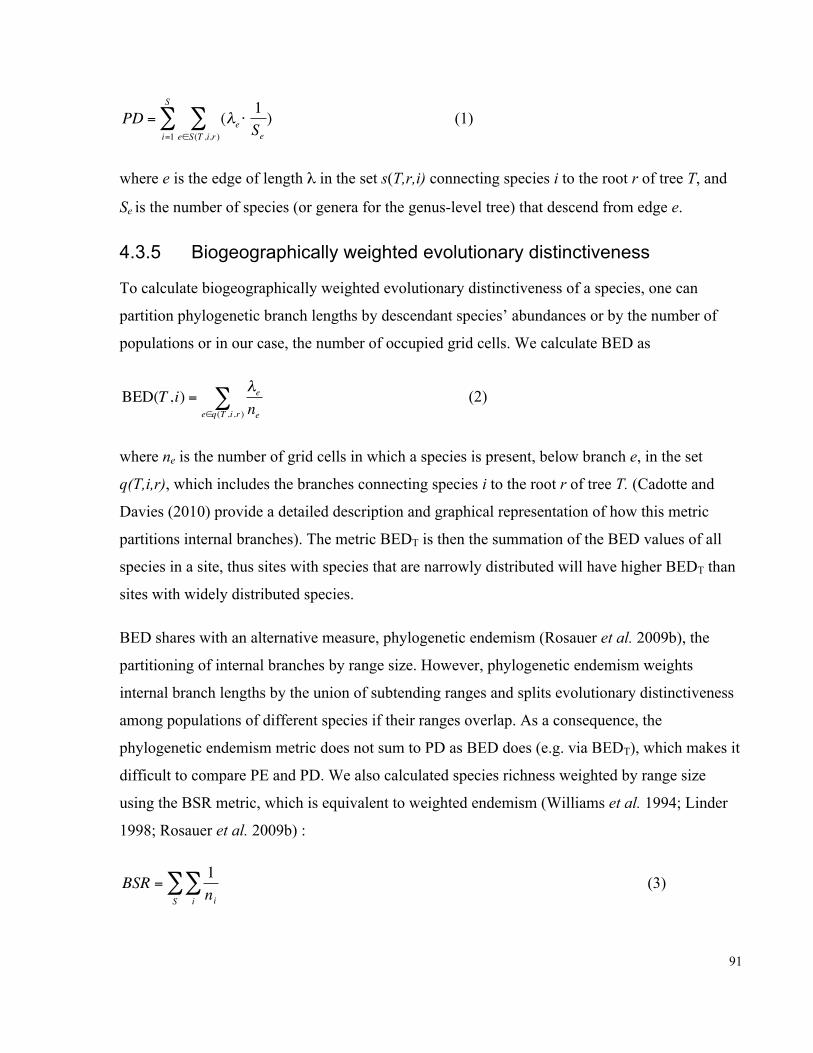
91
€
PD = (λe ⋅1See∈S(T ,i,r )
∑i=1
S
∑ ) (1)
where e is the edge of length λ in the set s(T,r,i) connecting species i to the root r of tree T, and
Se is the number of species (or genera for the genus-level tree) that descend from edge e.
4.3.5 Biogeographically weighted evolutionary distinctiveness
To calculate biogeographically weighted evolutionary distinctiveness of a species, one can
partition phylogenetic branch lengths by descendant species’ abundances or by the number of
populations or in our case, the number of occupied grid cells. We calculate BED as
BED(T ,i) = λenee∈q(T ,i,r )
∑ (2)
where ne is the number of grid cells in which a species is present, below branch e, in the set
q(T,i,r), which includes the branches connecting species i to the root r of tree T. (Cadotte and
Davies (2010) provide a detailed description and graphical representation of how this metric
partitions internal branches). The metric BEDT is then the summation of the BED values of all
species in a site, thus sites with species that are narrowly distributed will have higher BEDT than
sites with widely distributed species.
BED shares with an alternative measure, phylogenetic endemism (Rosauer et al. 2009b), the
partitioning of internal branches by range size. However, phylogenetic endemism weights
internal branch lengths by the union of subtending ranges and splits evolutionary distinctiveness
among populations of different species if their ranges overlap. As a consequence, the
phylogenetic endemism metric does not sum to PD as BED does (e.g. via BEDT), which makes it
difficult to compare PE and PD. We also calculated species richness weighted by range size
using the BSR metric, which is equivalent to weighted endemism (Williams et al. 1994; Linder
1998; Rosauer et al. 2009b) :
€
BSR =1nii
∑S∑ (3)
92
where i is the species, s is the number of species in the cell, and n is range size (in our case, the
number of cells occupied).
4.3.6 Metrics with genera-level tree
For all metrics (species richness, PD, BEDT, and BSR), we repeated the calculations at the level
of genus rather than species with the genera-level tree and site data aggregated across species at
each site. We examined the concordance among species richness, PD, BSR and BEDT with
Pearson correlation coefficients. We did not correct for spatial autocorrelation directly because
autocorrelation tends to strengthen the perceived relation between spatially structured variables,
whereas we were interested in departures between the various metrics; hence, our comparisons
are conservative.
Maps representing the distribution of species richness, PD, and BEDT values (all standardized at
mean[SD]=0 [1]) across the Cape Floristic Region were constructed in arcEditor (ESRI,
Redlands, California) with 8 quantile intervals from blue to red. The mapped values were derived
from the most conservative tree (low), where species lacking sequence data were included at low
evolutionary diversity position.
4.3.7 Reserve representation indices
We used a weighted index to compare how the prioritization of areas outside the current reserve
system differed when applying phylogenetic and species-diversity metrics. We weighted species
as an inverse function of the number of sites in which they were present were contained in
reserves. For species richness, this calculation was similar to BSR, except that the number of
sites in reserves was used instead of range size. We used a modification of the BEDT metric to
calculate the representation of phylogenetic richness in reserves. In this case, however, we
partitioned phylogenetic branch lengths by the number of sites a species occupied in the reserve
system, rather than by range size. Results were mapped for the Cape Floristic Region, using 8
quantile intervals from blue to red. The mapped values illustrated standardized (mean 0, SD 1)
values derived from the most conservative (low) tree, in which species lacking sequence data
included at low evolutionary diversity position.
93
To explore further the relation between evolutionary distinctiveness and range size, we plotted
one against the other (including only species for which sequence data were available)
4.4 Results
The cells analyzed in the Cape Floristic Region contained between 2 and 26 Proteaceae species
(mean [SD]=5.28 species [3.83]). Pearson’s correlation coefficients among the 3 metrics were
calculated separately for metrics from the no added species, lowest and highest evolutionary
distinctiveness and genus-level trees (Fig. 4-1). For the 4 trees, PD was strongly correlated with
species richness (r = 0.68-0.85), whereas the correlation between BEDT and species richness was
much weaker (r = 0.18-0.56). PD was similarly correlated with BEDT (r = 0.26-0.53). All
correlations were positive, but BEDT was distinct from the other metrics (Fig. 4-1).
The positioning of species missing phylogenetic information in the trees had little effect on the
relation between metrics, regardless of whether these species were added in positions of low or
high evolutionary distinctiveness (Fig. 4-1). However, metrics calculated with a tree resolved to
the level of genus resulted in different patterns of correlation than the equivalent values
calculated from the species-level tree. There was a stronger correlation between BEDT and PD (r
= 0.45) and BEDT and species richness (r = 0.37) and a weaker correlation between species
richness and PD (r = 0.67) for genus-level than for species-level trees.
To determine whether the distribution of BEDT values resulted only from the inclusion of
information on range size, independent of phylogeny, we compared BEDT with our metric BSR,
which incorporates both species richness and range size, but not phylogenetic branch lengths.
The correlation between the BSR and BEDT metrics was weak (r = 0.21-0.22, depending on how
species with missing sequence data were incorporated) (Fig. 4-1), which indicated BEDT’s
differential performance was the result of a nonrandom distribution of range size in relative to
evolutionary history. In addition, BSR was not correlated with species richness (r = -0.21).
Species richness and PD had similar spatial distributions. However, PD was less concentrated
than species richness such that many regions had moderate levels of phylogenetic diversity
whereas species richness tended to have high values in relatively fewer locations. The map of
BEDT showed far fewer areas of high diversity than the maps of either species richness or PD
94
and highlighted sites in the south and southwest as having higher diversity and thus higher
priority for conservation.
Species with high evolutionary distinctiveness tended to have smaller ranges, whereas a subset of
species with low evolutionary distinctiveness had very large ranges (Fig. 4-3b). However,
species’ range sizes were not correlated with relatedness (Blomberg’s Κ= 0.18, p>0.05), which
indicated close relatives did not tend to have similar range sizes.
The representation of species and phylogenetic diversity in the current reserve system differed
greatly. The correlation between the species and phylogenetic representation indices was not
significant (r = 0.17). Furthermore, the spatial distributions of these representation indices across
the region were strikingly different (Appendix 4-3). Few areas had a high concentration of
underrepresented species, and those that did were primarily near the southern border of the
region. There were numerous areas with high levels of underrepresented phylogenetic richness
near both the south and northeastern edges of the region.
4.5 Discussion
It is necessary to determine whether and when phylogenetic and species diversity represent
complementary or comparable information. We found that alternative metrics of diversity
emphasize different areas within the Cape Floristic Region of having high diversity, and that this
disconnect may provide additional information for conservation planning, such as in the selection
of areas for augmenting an existing reserve network. For example, the spatial distribution of our
multivariate metric, biogeographically weighted evolutionary distinctiveness (BEDT), which
incorporated both evolutionary distinctiveness and regional species rarity, departed from the
distribution of more traditional diversity metrics and highlighted additional areas (e.g., areas in
the southern edge of the region) that might be considered for protection, because they represent
areas with species that are both relatively distinct and rare compared the regional species pool.
Metrics accounting for evolutionary history may help identify sites overlooked by diversity
metrics that focus on species richness (Polasky et al. 2001; Forest et al. 2007). Divergence
between phylogenetic diversity (measured using PD) and species richness may be sizeable in
only particular cases, for example, when evolutionarily distinct species have narrow geographic
95
distributions and occur in species-poor sites (Rodrigues et al. 2005). Here, we found that
phylogenetic diversity and species richness are, unsurprisingly, strongly correlated in the Cape
Floristic Region. Nonetheless, their mapped values indicated species richness was concentrated
in fewer sites, which underrepresented the more spatially extensive distribution of phylogenetic
diversity, particularly in the eastern Cape Floristic Region. Significant differences among the
metrics were evident in the Cape Floristic Region even in the absence of a highly unbalanced
phylogeny or structured species distribution. Relatively few Proteaceae in the region have very
large or very small range sizes, and the phylogenetic tree we used was not greatly unbalanced (Ic
= 0.067, which is not significantly different than an equal-rates Markov null model [Ic = 0]. We
therefore suggest that even modest departures in tree shape or structuring of the distribution of
species ranges may therefore result in realized differences among metrics. In particular,
phylogenetic metrics and species richness can be decoupled when the focus is on sites within an
extensive region because sites may contain greatly different subsets of the species pool, which
would alter the shape of the tree (Cadotte & Davies 2010).
Forest et al. (2007) examined phylogenetic diversity for the entire Cape Floristic flora at a
coarser spatial grain than our analysis. Our results for patterns of divergence between species
richness and evolutionary diversity were similar to theirs. However, because Forest et al.
examined genus-level rather than species-level richness, it is possible their estimates of
phylogenetic diversity are biased downward because branching relations among species within
genera were not included. When we compared the relation between phylogenetic diversity and
species richness at the genus level, we observed an approximately 10% drop in correlation
strength compared with the species-level analyses, which may suggest the coarser taxonomic
resolution overestimated the mismatch between phylogenetic diversity and species richness.
Despite this difference in spatial and taxonomic resolutions between studies, our results were
generally congruent: phylogenetic diversity and species richness covaried closely when
considered in the absence of spatial context, but departed significantly in their spatial
distribution.
Metrics such as biogeographically weighted evolutionary distinctiveness, which combines
evolutionary diversity and rarity into a single measure of diversity, may allow a more holistic
approach to conservation prioritization. Nonrandom relations between evolutionary

96
distinctiveness and range size can produce rankings different from those of any single input
variable. Comparing biogeographically weighted evolutionary distinctiveness and
biogeographically weighted species richness allowed us to determine whether differences
between biogeographically weighted evolutionary distinctiveness and phylogenetic diversity
resulted simply from the incorporation of range-size information (in which case
biogeographically weighted evolutionary distinctiveness and biogeographically weighted species
richness should have a similar relation to the relation between species richness and phylogenetic
diversity) or from more complex relations between range size and evolutionary distinctiveness.
We found that biogeographically weighted evolutionary distinctiveness differed from the
similarly range size-weighted biogeographically weighted species richness, which suggests
evolutionarily distinct species tended to have more restricted geographical distributions. The
relation between evolutionary distinctiveness and range size could be of interest for species
conservation. Species that are evolutionarily distinct are of high conservation value (Crozier
1997), and species with small ranges have greater risk of extinction (Purvis et al. 2000a; Purvis
et al. 2000b; Cardillo et al. 2005). Although species-based prioritization schemes that
incorporate range size more likely emphasize these species, such schemes cannot differentiate
between species with small ranges that are not evolutionarily distinct and species that have small
ranges and are more evolutionary distinct (Davies et al. 2011).
Other metrics of phylogenetic diversity also incorporate measures of extinction risk (Redding &
Mooers 2006; Isaac 2007; Faith 2008a), but they rely on inferred estimates of extinction risk that
require detailed species data such as probability of extinction. In contrast, biogeographically
weighted evolutionary distinctiveness requires information only on range size (or abundance, or
population numbers, etc.), which is perhaps the most widely available type of species data. We
suggest biogeographically weighted evolutionary distinctiveness might therefore have much
greater practicality, especially for less well-described clades. Species prioritization rankings are
often developed at global or national scales, which means sites may be assigned a high priority
that may not contain the rarest species at the scale of interest.
A common criticism of alternative diversity metrics is that they are sensitive to the calculations
and the weighting scheme used to construct them. Although this criticism is valid, in fact
weighting schemes are implicit in all reserve-selection approaches (e.g., measures of species
97
richness simply assume all species have equal weights). Alternative weighting schemes allow
one to make explicit those aspects of biological diversity that are valued and further encourages
debate over what aspects of biological diversity should be valued. In addition, all metrics depend
on the calculations used to construct them. Comparing alternative metrics and performing
sensitivity analyses (here, differing phylogenetic construction methods) makes it clear that there
are differences in the distribution of biological diversity that are worth considering and that are
due to more than choice of metric construction alone.
The Protea Atlas Project (Rebelo 2001) produced one of the most detailed surveys of species
occurrence in the world (presence or absence of approximately 330 species over 36,000 sites).
These data are being used to guide reserve selection and predict how range sizes, locations, and
extinction risks will change as temperatures increase (Lombard et al. 2003; Midgley et al. 2003;
Bomhard et al. 2005). Proteaceae species in the Cape Floristic Region currently receive
considerable protection; the majority of species occur in at least one reserve. Our analyses are
primarily an illustration of how the distribution of evolutionary history can differ from the
distribution of species richness. Our results suggest that sites near the southern edge of the region
contain species that have high levels of evolutionary distinctiveness and limited ranges, but are
not assigned high conservation-priority rankings on the basis of species richness or phylogenetic
diversity. These areas in the south and southwest representing sites high in rare and evolutionary
distinct species may relate to the presence of lowland fynbos, which is restricted to areas
between the coast and interior mountains and has different vegetation than other fynbos types.
Many species in this region have small ranges, and mountains and coastal areas may form
barriers to dispersal. The resulting negative relationship between evolutionary distinctiveness and
range size that resulted in this area is important to consider because it means that in some cases
the species that capture the greatest evolutionary diversity will also be the species most
vulnerable to extinction. Further, modest differences in the distribution of phylogenetic and
species richness in the region may suggest different conservation scenarios for protecting
phylogenetic versus species richness and may lead to different conclusions regarding the future
positioning of protected areas.
98
References
Bilofsky, H. S., and C. Burks. 1988. The GenBank genetic sequence data bank. Nucleic Acids Research 16:1861-1864.
Bomhard, B., D. M. Richardson, J. S. Donaldson, G. O. Hughes, G. F. Midgley, D. C. Raimondo, A. G. Rebelo, M. Rouget, and W. Thuiller. 2005. Potential impacts of future land use and climate change on the Red List status of Proteaceae in the Cape Floristic Region, South Africa. Global Change Biology 11:1452-1468.
Cadotte, M. W., and T. J. Davies. 2010. Rarest of the rare: advances in combining evolutionary distinctivenss and scarcity to inform conservation at biogeographical scales. Diversity and Distributions, 16, 376-385.
Cardillo, M., G. M. Mace, K. E. Jones, J. Bielby, O. R. P. Bininda-Emonds, W. Sechrest, C. D. L. Orme, and A. Purvis. 2005. Multiple causes of high extinction risk in large mammal species. Science, 309:1239-1241.
Crozier, R. H. 1997. Preserving the information content of species: genetic diversity, phylogeny, and conservation worth. Annual Review of Ecology and Systematics 28:243-268.
Davies, T. J., G. F. Smith, D. U. Bellstedt, J. S. Boatwright, B. Bytebier, R. M. Cowling, F. Forest, L. J. Harmon, M. Musasya, B. D. Schrire, Y. Steenkamp, M. van der Bank, and V. Savolainen. 2011. Extinction risk and diversification are linked in a plant biodiversity hotspot. PLoS Biology 9(5): e1000620. doi:10.1371/journal.pbio.1000620.
Erwin, T. L. 1991. An evolutionary basis for conservation strategies. Science 253:750-752.
Faith, D. P. 1992. Conservation evaluation and phylogenetic diversity. Biological conservation 61:1-10.
Faith, D. P. 1994. Phylogenetic pattern and the quantification of organismal biodiversity. Philosophical Transactions of the Royal Society, London, B 345:45-58.
Faith, D. P. 2002. Quantifying biodiversity: a phylogenetic perspective. Conservation Biology 16:248-252.
Faith, D. P. 2008. Threatend species and the potential loss of phylogenetic diversity: conservation scenarios based on estimated extinction probabilities and phylogenetic risk analysis. Conservation Biology 22:1461-1470.
Fleishman, E., R. F. Noss, and B. R. Noon. 2006. Utility and limitations of species richness metrics for conservation planning. Ecological Indicators 6:543-553.
Forest, F., R. Grenyer, M. Rouget, T. J. Davies, R. M. Cowling, D. P. Faith, A. Balmford, J. Manning, S. Proches, M. van der Bank, G. Reeves, T. A. J. Hedderson, and V. Savolainen. 2007. Preserving the evolutionary potential of floras in biodiversity hotspots. Nature 445:757-760.
Gaston, K. J. 2003. The Structure and Dynamics of Geographic Ranges. Oxford University Press, Oxford, UK.
99
Goldblatt, P., and J. Manning. 2002. Plant diversity of the Cape Region of South Africa. Annals of the Missouri Botanical Garden 89:281-302.
Guindon, S., and O. Gascuel. 2003. A simple, fast, and accurate algorithm to estimate large phylogenies by maximum likelihood. Systematic Biology 52:696-704.
Harvey, P. H., and M. Pagel 1991. The Comparative Method in Evolutionary Biology. Oxford University Press, Oxford, UK.
Huang, J., B. Chen, C. Liu, J. Lai, J. Zhang, and K. Ma. 2011. Identifying hotspots of endemic woody seed plant diversity in China. Diversity and Distributions.
Isaac, N. J. B. 2007. Mammals on the edge: conservation priorities based on threat and phylogeny. PLoS ONE, 2(3): e296. doi:10.1371/journal.pone.0000296.
Jones, K. E., A. Purvis, and J. L. Gittleman. 2003. Biological correlations of extinction risk in bats. American Naturalist 161:601-614.
Lanave, C., G. Preparata, C. Saccone, and G. Serio. 1984. A new method for calculating evolutionary substitution rates. Journal of Molecular Evolution 20:86-93.
Larkin, M. A., G. Blackshields, N. P. Brown, R. Chenna, P. A. McGettigan, H. McWilliam, F. Valentin, I. M. Wallace, A. Wilm, R. Lopez, J. D. Thompson, T. J. Gibson, and D. G. Higgins. 2007. Clustal W and Clustal X version 2.0. Bioinformatics 23:2947-2948.
Linder, H. P. 1998. Historical interpretation of the African phytochoria. Pages 67-86 in C. R. Huxley, J. M. Lock, and D. F. Cutler, editors. Chorology, Taxonomy, and Ecology of the African and Madagascan Floras. Royal Botanical Gardens, Kew.
Lombard, A. T., R. M. Cowling, R. L. Pressey, and A. G. Rebelo. 2003. Effectiveness of land classes as surrogates for species in conservation planning for the Cape Floristic Region. Biological Conservation 112:45-62.
Midgley, G. F., L. Hannah, D. Millar, W. Thuiller, and A. Booth. 2003. Developing regional and species-level assessments of climate change impacts on biodiversity in the Cape Floristic Region. Biological conservation 112:87-97.
Mittermeier, R. A., and S. A. Cemex 2004. Hotspots revisited. CEMEX.
Moritz, C. 2002. Strategies to protect biological diversity and the evolutionary processes that sustain it. Systematic Biology 51:238-254.
Myers, N., R. A. Mittermeier, C. G. Mittermeier, G. A. B. da Fonseca, and J. Kent. 2000. Biodiversity hotspots for conservation priorities. Nature 403:853-858.
Polasky, S., B. Csuti, C. A. Vossler, and A. S. M. Meyers. 2001. A comparison of taxanomic distinctiveness versus richness as criteria for setting conservation priorities. Biological Conservation 97:99-105.
Purvis, A., J. L. Gittleman, G. Cowlishaw, and G. M. Mace. 2000a. Predicting extinction risk in declining specices. Proceedings of the Royal Society, B. 267:1947-1952.
Purvis, A., K. E. Jones, and G. M. Mace. 2000b. Extinction. Bioessays 22:1123-1133.
R Development Core Team. 2009. R: A Language and Environment for Statistical Computing. R Foundation for Statistical Computing. Vienna, Austria.
100
Raimondo, D. C., L. Von Staden, W. Foden, J. E. Victor, N. A. Helme, R. C. Turner, D. A. Kamundi, and P. A. Manyama. 2009. Red List of South African Plants. Strelitzia No. 25.
Rebelo, A. G. 2001. Sasol Proteas - a Field Guide to the Proteas of southern Africa. Fernwood Press, Vlaeberg.
Rebelo, A. G. 2002. Are we really finished atlassing. Protea Atlas Newsletter.
Redding, D. W., K. M. Hartman, A. Mimoto, D. Bokal, M. DeVos, and A. O. Mooers. 2008. Evolutionarily distinctive species often capture more phylogenetic diversity than expected. Journal of Theoretical Biology 251:606-615.
Redding, D. W., and A. O. Mooers. 2006. Incorporating evolutionary measures into conservation prioritization. Conservation Biology 20:1670-1678.
Regetz, J., M. W. Cadotte, and T. J. Davies. 2009. Ecologically-informed phylodiversity metrics. R-forge.
Rodrigues, A. S. L., and K. J. Gaston. 2002. Maximizing phylogenetic diversity in the selection of networks of conservation areas. Conservation Biology 16:674-682.
Rosauer, D., S. W. Laffan, M. D. Crisp, S. C. Donnellan, and L. G. Cool. 2009. Phylogenetic endemism: a new approach for identifying geographical concentrations of evolutionary history. Molecular Ecology 18:4061-4072.
Sanderson, M. J., D. Boss, D. Chen, K. A. Cranston, and A. Wehe. 2008. The PhyLoTA Browser: processing GenBank for molecular phylogenetics research. Systematic Biology 57:335-346.
Sauquet, H., P. H. Weston, C. L. Anderson, N. P. Barker, D. J. Cantrill, A. R. Mast, and V. Savolainen. 2009. Contrasted patterns of hyperdiversification in Mediterranean hotspots. Proceedings of the National Academy of Sciences of the United States of America 106:221-225.
Schultze, R. E. 1997. South African Atlas of Agrohydrology and Climatology. Water Research Commission, Pretoria.
Sechrest, W., T. M. Brooks, G. A. B. da Fonseca, W. R. Konstant, and R. A. Mittermeier. 2002. Hotspots and the conservation of evolutionary history. Proceedings of the National Academy of Sciences of the United States of America 99:2067-2071.
Vane-Wright. 1991. What to protect - systematics and the agony of choice. Biological conservation 55:235-254.
Williams, P. H., C. J. Humphries, P. L. Forey, and R. I. Vane-Wright. 1994. Biodiversity, taxonomic relatedness, and endemsm in conservation. Page 438 in P. L. Forey, C. J. Humphries, and R. I. Vane-Wright, editors. Systematics and Conservation Evaluation. Oxford University Press, Oxford, UK.

101
Figures
Figure 4-1. Pearson correlation coefficients showing the strength of the relationships
among species richness, phylogenetic diversity (PD), and biogeographically weighted
evolutionary distinctiveness (BEDT) metrics for Proteaceae in the Cape Floristic Region,
South Africa (none, species lacking sequence data not included; low, species lacking
sequence data included at low evolutionary diversity position; high, species lacking
sequence data included at high evolutionary diversity position; genera, resolved only to the
level of genus).
The inset shows the Pearson correlation coefficients between the 2 range-weighted metrics
(biogeographically weighted evolutionary distinctiveness and biogeographically weighted
species richness (BSR)) for the none, low, and high trees.

102
Figure 4-2. Proteaceae diversity of 311 species in the Cape Floristic Region on the southern
tip of Africa, diversity is measured using (a) species richness, (b) phylogenetic diversity,
and (c) biogeographically weighted ecological distinctiveness, where (b) and (c) were
calculated using the low tree, where species lacking sequence data were included at low
evolutionary diversity position.
All diversity measures are scaled with mean 0 and SD 1. Colors are scaled over 8 quantile
intervals from blue (low diversity) to red (high diversity).

103
Figure 4-3. (a) The relation between biogeographically weighted evolutionary
distinctiveness (BEDT) and range size (calculated as the square-root transformed number
of cells occupied by the species) and (b) distribution of range size for the ‘none’
phylogenetic tree, where Proteaceae species lacking species data are not included.
104
Appendices
Appendix 4-1. Phylogenetic tree of the CFR Proteaceae, constructed using sequences from
Genbank.
(Martin & Dowd 1991; Martin & Dowd 1993; Nickrent & Soltis 1995; Hoot & Douglas 1998;
Hoot et al. 1999; Parkinson et al. 1999; Qiu et al. 1999, 2000; Fishbein et al. 2001; Barker et al.
2002; Mast & Givnish 2002; Moisen & Frescino 2002; Soltis et al. 2003; Barker et al. 2004;
Kim et al. 2004; Mast et al. 2004; Reeves et al. 2004; Pharmawati et al. 2005; Qiu et al. 2005;
Qiu et al. 2006; Redding & Mooers 2006; Wright et al. 2006; Chase et al. 2007; Worberg et al.
2007; Holmes et al. 2008; Lahaye et al. 2008; Mast et al. 2008; Ford et al. 2009; Group 2009;
Royas-Jimenez et al. 2009; Sauquet et al. 2009; Wang et al. 2009; Gillman et al. 2010; Qiu et al.
2010; Valente et al. 2010).

105

106
Appendix 4.1 References for phylogeny
1. Martin PG & Dowd JM (1991) A comparison of 18s ribosomal RNA and rubisco large subunit sequences for studying angiosperm phylogeny. Journal of Molecular Ecology 33(3):274-282.
2. Martin PG & Dowd JM (1993) Partial sequence of ribosomal RNA of Papilionaceae and related families. Phytochemistry 33:361-363.
3. Nickrent DL & Soltis DE (1995) A comparison of angiosperm phylogenies from nuclear 18S rRNA and rbcL sequences. Annals of the Missouri Botanical Garden 82(2):208-234.
4. Hoot SB & Douglas A (1998) Phylogeny of the Proteaceae based on atpB and atpB/rbcL intergenic spacer region sequences Australian Systemic Botany, 11(4), 301-320.
5. Parkinson CL, Adams KL, & Palmer JD (1999) Multigene analyses identify the three earliest lineages of extant flower plants. Unpublished.
6. Qiu YL, et al. (1999) The earliest angiosperms: evidence from mitochondrial, plastid and nuclear genomes. Nature 402:404-407.
7. Hoot SB, Magallon S, & Crane PR (1999) Phylogeny of basal eudicots based on three molecular data sets: atpB, rbcL, 18S nuclear ribosomal DNA sequences. Annals of the Missouri Botanical Garden 86:1-32.
8. Qiu YL, et al. (2000) Phylogeny of basal angiosperms: analyses of five genes from three genomes. International Journal of Plant Sciences 161(S6):S3-S27.
9. Fishbein M, Hibsch-Jetter C, & Hufford L (2001) Phylogeny of Saxifragales (angiosperms, eudicots): analysis of a rapid, ancient radiation. Systematic Biology 50(6):817-847.
10. Moisen GG & Frescino TS (2002) Comparing five modelling techniques for predicting forest characteristics. Ecological Modelling 157(2-3):209-225.
11. Mast AR & Givnish TJ (2002) Historical biogeography and the origin of stomatal distributions in Banksia and Dryandra (Proteaceae) based on their cpDNA phylogeny. American Journal of Botany 89(8):1311-1323.
12. Barker NP, Weston PH, Rourke JP, & Reeves G (2002) The relationships of the southern African Proteaceae as elucidated by internal transcribed spacer (ITS) DNA sequence data. Kew Bulletin 2002.
13. Soltis DE, et al. (2003) Gunnerales are sister to other core eudicots: implications for the evolution of pentamery. American Journal of Botany 90(3):461-470.
14. Mast AR, Jones EH, & Havery SP (2004) An assessment of the DNA sequence evidence for the paraphyly of Banksia with respect to Dryandra (Proteaceae). Unpublished.
15. Reeves G, Barraclough TG, Rebelo AG, Fay MF, & Chase MW (2004) Molecular phylogenetics of African Protea: evidence from DNA sequences and AFLP markers for a Cape origin. Unpublished.
107
16. Barker NP, Vanderpoorten A, Morton CM, & Rourke JP (2004) Phylogeny, biogeography, and the evolution of life-history traits in Luecadendron (Proteaceae). Molecular Phylogenetics and Evolution 33(3):845-860.
17. Kim S, Soltis DE, Soltis PS, Zanis M, & Suh Y (2004) Phylogenetic relationships among early-diverging eudicots based on four genes: were the eudicots ancestrally woody? Molecular Phylogenetics and Evolution 31(1):16-30.
18. Qiu YL, et al. (2005) Phylogenetic analyses of basal angiosperms based on nine plastid, mitochondrial, and nuclear genes. International Journal of Plant Sciences 166(5):815-842.
19. Pharmawati M, Yan G, & Finnegan PM (2005) The conservation of mitochondrial genome sequence in Luecadendron (Proteaceae). Unpublished.
20. Wright S, Keeling J, & Gillman L (2006) The road from Santa Rosalia: a faster tempo of evolution in tropical climates. Proceedings of the National Academy of Sciences of the United States of America 103(20):7718-7722.
21. Qiu YL, et al. (2006) Reconstructing the basal angiosperm phylogeny: evaluating information content of mitochondrial genes. Taxon 55(4):837-856.
22. Worberg A, et al. (2007) Phylogeny of basal eudicots: insights from non-coding and rapidly evolving DNA. Organism Diversity and Evolution 7(1):55-77.
23. Chase MW, Cowan RS, Hollingsworth PM, & Conrad F (2007) Unpublished.
24. Mast AR, Willis CL, Jones EH, Downs KM, & Weston PH (2008) A smaller Macadamia from a more vagile tribe: inference of phylogenetic relationships, divergence times, and diaspore evolution in Macadamia and relative (tribe Macadamieae; Proteaceae). American Journal of Botany 95(7).
25. Holmes GD, Blacket MJ, James EA, & Hoffmann AA (2008) Molecular phylogenetic analysis of the Grevillea aquifolium (Proteaceae) group of species. Unpublished.
26. Lahaye R, et al. (2008) DNA barcoding the floras of biodiversity hotspots. Proceedings of the National Academy of Sciences of the United States of America 105(8):2923-2928.
27. Sauquet H, et al. (2009) Contrasted patterns of hyperdiversification in Mediterranean hotspots. Proceedings of the National Academy of Sciences of the United States of America 106(1):221-225.
28. Wang W, Lu AM, Ren Y, Endress ME, & Chen ZD (2009) Phylogeny and classification of Ranunculales: Evidence from four molecuar loci and morphological data. Perspectives in Plant Ecology, Evolution, and Systematics 11:81-110.
29. Ford CS, et al. (2009) Selection of candidate coding DNA barcoding regions for use on land plants. Botanical Journal of the Linnean Society 159(1):1-11.
30. Group CPW (2009) A DNA Barcode for Land Plants. Unpublished.
31. Royas-Jimenez K, Vindas-Rodriguez M, & Tamayo-Castillo G (2009) Evaluation of three chloroplastic markers for barcoding and for phylogenetic reconstruction purposes in native plants of Costa Rica. Unpublished.

108
32. Gillman LN, Keeling J, Gardner RC, & Wright SD (2010) Faster evolution of highly conserved DNA in tropical plants. Unpublished.
33. Valente LM, et al. (2010) Diversification of the african genus protea (proteaceae) in the cape biodiversity hotspot and beyond: equal rates in different biomes. Evolution 64(3):745-760.
34. Qiu YL, et al. (2010) Angiosperm phylogeny inferred from sequences of four mitochondrial genes. Journal of Systematics and Evolution 48:391-425.
35. Redding DW & Mooers AO (2006) Incorporating evolutionary measures into conservation prioritization. Conservation Biology 20:1670-1678.
Appendix 4-2. Graphical representation of how a species, D, lacking sequence data, would
be positioned on the phylogenetic tree, based on branch lengths, relative to its congeners A,
B, and C with sequence data.
a) The species tree based only on species with sequence data; b) the high tree with D in a
polytomy with its most evolutionarily distinct congener A, and c) the low tree with D in a
polytomy with its most evolutionarily distinct congeners (B and C).
‘none’ ‘high’ ‘low’

109
Appendix 4-3. Reserve representation index for 311 species of Proteaceae in the Cape
Floristic Region, a biodiversity hotspot on the southern tip of Africa. The maps illustrate
prioritization of a, species diversity or b, phylogenetic diversity, outside of reserve sites:
Phylogenetic or species diversity is scaled by degree of representation within the existing
reserve network species to highlight remaining areas with less represented phylogenetic or
species diversity (see Methods).
Measures are scaled with mean 0 and standard deviation 1; colors are scaled over eight quantile
intervals from blue to red, and increase as the degree of underrepresented diversity in a site
increases. The current system of reserves is shown in green. See text for additional details.

110
Copyright Acknowledgements
Tucker, C.M., Cadotte, M.W., Davies, T.J., Rebelo, A.G. 2012. The distribution of biodiversity:
linking richness to geographical and evolutionary rarity in a biodiversity hotspot. Conservation
Biology, Volume 26, No. 4, 593–601
2012 Society for Conservation Biology
111
Chapter 5 Unifying measures of biodiversity: understanding when richness
and phylogenetic diversity should be congruent
5 5
5.1 Abstract
Aim: Biogeographical theory and conservation valuation schemes necessarily involve assessing
how biodiversity is distributed through space, and ‘biodiversity’ encapsulates many different
aspects of biological organization and information. While biogeography may try to explain
biodiversity patterns, successful conservation strategies should attempt to maximize different
aspects of diversity. Ultimately, diversity patterns are the product of evolutionary history, and
research and conservation efforts seek to understand the unequal distribution of evolutionary
history. For conservation efforts, results have been inconsistent as to whether species richness
provides sufficient surrogacy for evolutionary history. Here we provide a conceptual framework
allowing for the direct comparison of taxonomic richness and phylogenetic diversity, both in
terms of their mechanistic relationship, and the relationship between their spatial distributions.
Location: Global
Methods: We present a framework that relates regional species richness, phylogenetic diversity,
biogeographically weighted evolutionary distinctiveness, and biogeographically weighted
species richness. Further, we use simulations to illustrate how the size of the species pool,
topological patterns within the phylogeny, and autocorrelation in spatial distributions affect the
correlation among metrics.
Results: In regions that include both recently diversified groups and ancient species poor
lineages, large species pools and low spatial autocorrelation, the correlation between biodiversity
measures is lower than regions with low richness, balanced phylogenetic trees and high spatial
autocorrelation.
Main conclusions: We can now understand and predict when regional richness and phylogenetic
diversity should be strongly correlated. This congruency is the product of evolutionary and

112
ecological processes that determine species pool membership and community assembly. Further,
in regions where species richness is not expected to be congruent with phylogenetic
distinctiveness, re-examining how existing reserve networks protect the multiple aspects of
biodiversity is critically important.
5.2 Introduction
Global patterns of biological diversity reveal stark contrasts. Some regions contain thousands of
species in relatively small areas, whereas elsewhere there may only be a few species over
extremely large areas. Understanding this inequality in the distribution of species has been the
focus of the creative energy of numerous scientists (e.g. MacArthur & Wilson 1967; Gaston &
Blackburn 2000) and has served as the basis of global conservation prioritization (Myers et al.
2000; Fleishman et al. 2006). The recognition that the term diversity is not synonymous with
species richness, but instead encompasses organismal variety at all levels, from genetic variation
to the differences in the richness of higher taxa, and includes the diversity in ecosystem structure
and function (Wilson & Peter 1988), has led researchers to measure the spatial distribution of
different aspects of diversity (Faith 1992; Forest et al. 2007; Devictor et al. 2010; Huang et al.
2011; Tucker et al. 2012a). Such comparisons aim to understand the biogeographical relationship
between different facets of diversity. This type of research has been motivated, in part, by the
fact that historically reserves have not focused on aspects of diversity beyond richness and
endemism. Therefore it is reasonable to examine the efficacy of existing reserves in protecting
other facets of biodiversity (Devictor et al. 2010; Huang et al. 2011; Tucker et al. 2012a). In
addition, comparing different biogeographical distributions of diversity allows researchers to
potentially infer different mechanisms generating and maintaining different aspects of diversity.
For example, studies examining latitudinal gradients of species richness often infer the influence
of climate on speciation rates (Weir & Schluter 2007), whereas biogeographical studies that
focus on genetic diversity often find that vicariance or natural barriers are critically important
(Kuo & Avise 2005).
There is a long history of measuring and mapping patterns of species richness across
biogeographical regions throughout the world (Wallace 1876; Whittaker 1954; Preston 1960;
Whittaker 1960; Stevens 1989). As the importance of alternative forms of diversity is
113
increasingly recognized (Faith 1992, 1994; Diaz & Cabido 2001; 2010; Cadotte et al. 2011),
documenting patterns of other measures of diversity such as phylogenetic and functional
diversity become an important exercise. For diversity and conservation research, having a precise
estimate of ecological or functional diversity is beneficial. However, ecologically-meaningful
functional diversity is often difficult to quantify due to a lack of comprehensive trait information
for species in a region, or an incomplete understanding of how traits correspond to ecological
differences.
A related measure that is used as a surrogate for functional diversity is that of phylogenetic or
evolutionary diversity, which quantifies the amount, distribution or evenness of evolutionary
information contained within species assemblages. There are a number of ways to measure
phylogenetic diversity in communities (Webb et al. 2002; Cavender-Bares et al. 2009; Cadotte et
al. 2010b), but methods that quantify either the amount of evolutionary history or the
evolutionary distinctiveness of a set of species are most appropriate to examine spatial patterns
of diversity (Faith 1992; Isaac 2007; Cadotte & Davies 2010; Davies & Cadotte 2011). The most
often used measure is Faith’s (1992) phylogenetic diversity (PD), which is the sum of all
phylogenetic branch lengths connecting species together. Evolutionary distances are often
correlated with potential multidimensional phenotypic differences among species (Vane-Wright
et al. 1991; Faith 1992). There are many subtleties associated with this assumption, including the
degree of phylogenetic conservatism among traits and the degree that trait divergence follows
Brownian motion evolution. Specific traits and lineages often fail to meet these assumptions and
some researchers have found functional diversity and phylogenetic diversity vary independently
(Safi et al. 2011). Regardless, researchers often use phylogenetic information to represent
unknown aspects of species ecologies or simply as a representation of similarities in the
information contained within their genomes. To this end, a number of studies have examined the
spatial distribution of phylogenetic diversity and delineate sites with disproportionately high
phylogenetic diversity (Moritz 2002; Rodrigues & Gaston 2002; Forest et al. 2007; Devictor et
al. 2010; Tucker et al. 2012a).
On its own, species richness is not ecologically meaningful, and considering other forms of
diversity which capture species differences becomes important. With a particular focus on
conservation, a number of studies have questioned the efficacy of richness as a surrogate for

114
other types of diversity and have called for more multifaceted approaches to conservation
(Crozier 1997; Bonn & Gaston 2005; Fleishman et al. 2006; Devictor et al. 2010; Davies &
Cadotte 2011). Studies that examine the congruence between species (or generic) and
phylogenetic diversity have been inconsistent. For example, Devictor et al. (2010) found a large
spatial mismatch between the species, functional and phylogenetic diversity of birds across
France; these measures were congruent in some areas, and incongruent in others, possibly
depending on the history of the regional species pool in each area. They found that phylogenetic
and functional diversity were underrepresented in the current reserve network, relative to species
richness. Two papers which compared the spatial distribution of generic or species diversity in
the Cape Floristic Region of South Africa (Forest et al. 2007; Tucker et al. 2012a) similarly
found evidence of spatial incongruence between species richness and phylogenetic diversity.
Conversely, several studies found that phylogenetic diversity and taxonomic diversity to have
similar spatial distributions: for example, Rodrigues and Gaston (2002) found that phylogenetic
and generic richness of birds in northwest South Africa showed high spatial congruence, and
reserve site selection was complementary. Perez-Losada and colleagues (2002) found little
difference in conservation priorities for Chilean freshwater crabs, regardless of whether species
richness or phylogenetic diversity was considered (though Faith & Baker 2006 raise doubts about
these results). Similar conclusions were made regarding Ozark crayfishes (Crandall 1998). This
marked variation in the observed relationship between species richness and phylogenetic
diversity appears to makes it difficult to draw conclusions regarding the relationship between
these measures.
The relationship between phylogenetic diversity and species diversity depends on the
phylogenetic topology and the geographic distribution of species (Rodrigues et al. 2005). For
example, in regions with large, diverse species pools, particularly in the case of randomly
accumulating species, phylogenetic diversity increases at a similar rate as species richness, and
thus phylogenetic diversity is likely to be highly correlated with species richness (Fjeldsa 1994;
Mace et al. 2003). This suggests that a framework predicting the degree of correlation expected
between different measures of diversity could make an important contribution to our
understanding of the biogeographical distribution of diversity.

115
While there has been substantial effort to measure alternative aspects of diversity, there is a
surprising dearth of studies that explicitly incorporate abundances into phylogenetic metrics of
any kind (but see: Cadotte et al. 2010c; Scheiner 2012). Given the importance of species range
sizes and abundances for understanding basic biogeographical processes as well as their role in
extinction risk, this is an area that deserves further study. One method of weighting richness by
abundances, here referred to as ‘biogeographically-weighted species richness’ (BSR)1, which
sums the inverse of the range sizes, or number of sites or populations of all species at a site or in
a region as: , where S is the number of species at a specific site and ni is the number
of sites (or populations or range size) that species i occurs at over the larger region (Crisp et al.
2001; Rosauer et al. 2009b). Thus BSR is small if a site contains species with large ranges, and is
large if the site has many range-restricted species. A measure like BSR may show quite different
patterns than non-range size related measures of diversity, especially if rich sites
disproportionately contain large-ranged or abundant species (Rosauer et al. 2009a; Tucker et al.
2012b).
Measures of phylogenetic diversity may also provide additional information when they
incorporate range-size. When Isambert and colleagues (2011) examined phylogenetic diversity
patterns in Malagasy national parks, they found that phylogenetic diversity was negatively
correlated with numbers of endemic species, as these endemics are the product of recent species
radiations in Madagascar. Abundance information is straightforward to incorporate into
phylogenies, because stopping a phylogenetic tree at the species level is arbitrary, and a tree can
be resolved to the individual or population level by extending the tree via adding further tips
(Cadotte et al. 2010c). (In cases where additional genetic information is not available for
individuals or populations, intraspecific tips can still be added as uninformative polytomies). As
a result, the evolutionary distinctiveness of a species would explicitly account for the numbers of
individuals or populations, and therefore a measure of extinction risk. Several weighted
1 Crisp and colleagues referred to this metric as ‘weighted endemism’ (WE) and we refer to it as BSR to make the terminology comparable to the other measures in this paper and because endemism is a scale dependent measure with specific connotations.
BSR = 1nii=1
S
!

116
phylogenetic diversity metrics have been proposed that explicitly incorporate species abundances
or range sizes into prioritization schemes (Rosauer et al. 2009b; Cadotte & Davies 2010). There
are other useful measures that use extinction risk (Redding & Mooers 2006; Faith 2008b) or
IUCN species ranks (Isaac 2007) to weight phylogenetically-based prioritization. IUCN ranks
and extinction risk are used because of the availability and accessibility of this data and the fact
that such conservation ranks are based on abundance and range size.
An example of a metric that combines evolutionary distinctiveness with abundances is the BED
metric (Cadotte & Davies 2010), which partitions internal branches in a phylogenetic tree by the
range or population size of the subtending taxa: , where ne is the number
of grid cells in which a species is present, below branch e, of length λ , in the set q(T,i,r), which
includes the branches connecting species i to the root r of tree T. (Cadotte and Davies [2010]
provide a detailed description and graphical representation of how this metric partitions internal
branches –see also Fig. 1d). It should be noted that how abundances are calculated (e.g., number
of sites occupied versus geographical extent versus total number of individuals) can affect BED
values and their interpretation, and researchers should be cognizant of the potential implications
of their measure of rarity (Rabinowitz 1981). Species with long branches and low abundances or
ranges are weighted highly (i.e. distinct and rare), while species that share the majority of their
genetic heritages with many other species, and have high abundances receive less weight. As a
result, in a biogeographic setting, BED highlights sites containing species that have greater
extinction risk and also have few close relatives.
5.3 Unifying biodiversity measures
Given seemingly contradictory results from empirical studies (Rodrigues & Gaston 2002; Forest
et al. 2007; Devictor et al. 2010; Tucker et al. 2012a), reconciling results from different
biodiversity metrics, and further, predicting how these differing metrics will relate is clearly
necessary. There have only been a few studies published that investigate the effect of
phylogenetic topology and abundance distributions on the relationship between phylogenetic and
species based metrics of diversity (Rodrigues et al. 2005; Schweiger et al. 2008), and there
remains a need for frameworks relating phylogenetic diversity with species richness (whether
!
!
BED(T,i) ="enee#q(T ,i,r)
$

117
they are weighted by abundance or not). Comparing the spatial distributions of biodiversity
measures informs conservation decision-making because incongruence between measures
highlights how different aspects of diversity (species richness, evolutionary history, geographical
rarity) are differentially distributed through space. It also provides an opportunity to understand
why patterns of diversity vary among biogeographic regions. In the following, we present a
conceptual unification of these measures, and then explore the effects of 1) tree structure, 2)
spatial structure, 3) species pool size on the relationship between diversity metrics.
5.3.1 Conceptual underpinning of biodiversity measures
It is relatively straightforward to compare counts of the number of species with Faith’s
phylogenetic diversity. Metrics based on species richness (SR) implicitly assume that species are
all equally weighted (weight of 1). This is synonymous to a phylogenetic tree where the
phylogenetic relationships are removed and the tip to root distance is equal to 1 for an ultrametric
tree (Fig. 1a) –that is, a star phylogeny where all terminal branches originate from a single
polytomy (Helmus et al. 2007). If an informative ultrametric phylogeny is also scaled with a tip
to root length of 1 (Fig. 1b) then the more distantly related the individual species, the closer the
value of PD is to SR. The alternative scaling method would be to multiply species richness by
the real tip to root distance from the phylogeny. Regardless of the scaling method, PD will
diverge from SR as the tree becomes increasingly imbalanced and as the mean nearest neighbour
distance decreases. Thus in regions with incongruent site rankings between PD and SR, we
should expect less balanced evolutionary relationships among species.
When we weight the branches by species abundances or range sizes for BSR or BED (Fig. 1c, d),
then there is a second axis to compare. BED can deviate from SR due to topology, abundance or
their combined effect. Thus BED must be compared to both PD and BSR in order to draw
conclusions about the mechanisms that affect diversity distributions. Like the relationship
between SR and PD, when the phylogeny is relatively balanced and has long terminal branches,
the expectation is that BSR and BED give similar values. Both BSR and BED sum to their
unweighted counterparts when each species value is multiplied by its abundance, for example:
or PD is approximated by: where S is the number of species or !
!
PD = ni " BEDii
S
#!
!
n ni " BEDii
S
#
118
terminal tips in the phylogeny and n is a measure of abundance. Thus, if abundance lacks
variation (i.e., all species have roughly equivalent abundances) then PD and site summed BED
values are highly correlated.
5.3.2 Exploring the correlation between metrics
The four biogeographical measures of diversity considered here (Fig. 5-1) can vary from one
another depending on the topology of the phylogeny and the geographical ranges sizes or
abundances of species. We now ask how variation in these aspects can affect the strength of the
correlation between metrics. To do this, we simulated thousands of trees and abundance
distributions (see Appendix 5-1 for full methodology) and compared the four diversity metrics.
Specifically, we assess whether variation in topology, the strength of the spatial autocorrelation
in species occupancy patterns and species pool size have consequences for the strength of the
relationship between richness and phylogenetic measures of diversity.
5.3.3 Tree structure
If all species are equally related in a polytomy or star phylogeny (i.e. all species have identical
amounts of unshared evolutionary information), with tip to root branch lengths equal to 1, then
SR and PD are equivalent (e.g., Fig. 1). When a tree’s topology diverges from that of a star
phylogeny (as is common), so that information is no longer symmetrically distributed through
clades and/or through time (see Fig. 2), we can expect systematic changes in the relationship
between SR and PD.
In trees with proportionally more information in the terminal branches –that is, when there are
few recent radiations (Fig. 2)--SR and PD should be highly correlated. A star phylogeny is the
extreme of this situation, in which internal branches are minimized so the ratio between branch
number and species number approaches one, at which point SR and PD are equivalent (Fig. 3).
This suggests that in communities with species from anciently diverged lineages (Hawkins et al.
2006; Lopez-Fernandez & Albert 2011) or where community assembly selects distantly related
species (Webb 2000; Webb et al. 2002), we would expect stronger correlations between SR and
PD. Conversely, when trees have long internal branches and many short terminal branches
representing recent speciation events (e.g. the Cape Flora, Linder 2005; cichlids, Seehausen
2006) or assembly processes that select for clades of closely related species (Cadotte et al.

119
2010a; Helmus et al. 2010), the correlation between SR and PD should be weaker. When the
evolutionary information in the tree is biased towards particular clades—i.e. some clades contain
more evolutionary diversity than others—the correlation between SR and PD is also weakened
(Fig. 3). Asymmetrical trees are likely more common in some regions with a long history of
climatic or geological instability, as diversity in these regions is largely defined by unequal or
temporally contingent speciation and extinction rates (Stebbins 1974; Weir & Schluter 2007).
Symmetrical trees may be more likely in regions in which rates of extinction and speciation are
relatively similar or more stable, such as in the tropics (Hawkins et al. 2006; Weir & Schluter
2007).
The relationship between the two abundance-weighted metrics (BSR and BED) is also dependent
on the shape of the phylogenetic tree. A symmetrical tree with long internal branches yields a
stronger correlation between BSR and BED (Fig. 4a-i,iii). This is because short terminal
branches (recent radiations) minimizes the variation in evolutionary diversity, so that BSR and
BED are more similar. In addition, the strength of the correlation between range size and
evolutionary distinctiveness alters the correlation between BSR and BED (Fig. 4a-ii). When
range size and evolutionary distinctiveness are negatively correlated, i.e. rare species do not tend
to be distinct and vice versa, the correlation between BSR and BED is stronger. This is because
the relationship between BSR and BED is weakened when rare species also tend to be distinct
and so receive high BED values, causing BED values to diverge from the abundance weighted--
but not phylogenetically informed--BSR metric.
Similarly, the abundance weighted BED metric should have predictable relationships with PD
and SR depending on the topology of the phylogenetic tree. In addition to the shape of the tree,
the distribution of the abundance information in relation to the phylogenetic branch lengths
changes the relationship between BED and PD. The correlation between BED and PD should be
strongest under those conditions that minimize the importance of the abundance weighting (as
previously, when there is a negative correlation between range size and evolutionary
distinctiveness)(Fig. 4b-ii), and when the phylogenetic tree has long terminal branches and high
symmetry (Fig. 4b-i,iii).

120
5.3.4 Spatial structure and abundance distribution
The spatial structure of species ranges in a region can alter the expected relationship between the
different types of diversity. We examined the role of spatial structure in species’ ranges, in
particular the likelihood that conspecifics be present in neighbouring sites. High autocorrelation
in species presences’ tends to result in small, compact ranges, whereas low autocorrelation
results in patchy but larger ranges. This spatial structure can create variation in the spatial
distribution overall of species richness. High autocorrelation could be reflected in the clumped
distribution of tropical tree species, for example, while in other forests species might be highly
dispersed, representing a system with low autocorrelation in species presences (Condit et al.
2000). The correlation between metrics tends to be lowest when there is low spatial
autocorrelation in species presences (Appendix 5-2, A). When spatial autocorrelation is low, the
distribution of evolutionarily distinct species is more uneven through space, meaning that some
sites may contain more phylogenetic information despite containing fewer species, and this
weakens the relationship between the different metrics.
The distribution of species abundances should also affect the relationship between the SR, PD
and the abundance weighted BED and BSR metrics. When the relative abundance distribution is
uniform (e.g. each abundance is equally likely to be observed), the correlation between
abundance-weighted BED and BSR with SR and PD metrics should be highest. As the
abundance distribution reflects the more realistic scenario in which most species have low
abundances, and increasingly few species have high abundances (often represented with a log-
normal distribution), abundance-weighted and non-abundance-weighted metrics will diverge.
5.3.5 Species pool size
The number of species in the regional species pool impacts the strength of the correlations
between metrics. When species pools are small, the correlation between PD and SR is stronger,
since communities contain relatively few species and proportionally more of the species pool;
this means that the subtree for that community is relatively depauperate and the importance of
tree shape is minimized (Appendix 5-2, B). Only for relatively large regional pools, above about
80 species, do sites with very low SR-PD correlations regularly appear. PD will always be highly
correlated with SR for regional pools with relatively few species.
121
While species pool size has important consequences for PD-SR correlations, it is much less
consequential for metrics that incorporate species range sizes or abundances. The effect of the
abundance distribution or the degree of autocorrelation in species occupancy patterns is critically
important for the abundance-weighted metrics and appears to mask any effect of the pool size.
5.4 Conclusions: Securing the place for evolution and rarity in conserving biodiversity
If we are to conserve the diversity of life on Earth, then biodiversity conservation is an
invaluable endeavour. It necessarily involves emphasizing or accommodating multiple priorities
including social and economic valuations (Meffe & Viederman 1995), the functioning of
ecosystems and accounting for the services they provide (Chan et al. 2006), and the preservation
of the diversity of life. Conservation efforts have focused on numerous aspects of diversity and
have produced conflicting priorities (Fleishman et al. 2006). Species diversity, composition,
rarity and evolutionary distinctiveness are three important aspects of diversity that are often
considered, and conceptual approach that provides a meaningful way to compare differing
aspects of diversity is of value. While incongruities in biodiversity metrics can highlight
additional sites to protect in a conservation network (Forest et al. 2007; Devictor et al. 2010;
Tucker et al. 2012a), understanding how and why metrics diverge is important for larger scale
conservation schemes, as well as informing our basic understanding of the evolutionary and
ecological processes generating patterns of biodiversity. With a priori knowledge about several
aspects of diversity, such as basic information about the evolutionary topology, species pool size
or how species are distributed through space; one can predict whether different metrics should be
weakly or strongly correlated (Fig. 5). This in turn would inform the types of diversity that
should be prioritized in conservation assessments, as well as inform hypotheses about the
processes behind the origin and maintenance of diversity in a region.
Two studies that conclude that SR and PD are highly correlated, and thus recommend using SR
as a surrogate for PD (Rodrigues et al. 2005; Rodrigues et al. 2011b), can be contextualized
given our understanding of how topology and species distributions affect SR-PD correlations. In
one of these studies, which examines the surrogate value of SR for PD using an artificially
simulated set of species and phylogenetic data (Rodrigues et al. 2005), the species pool chosen

122
was quite small –about 16 species. Given the influence of pool size on the strength of the
correlations (Supplementary figure 1 ), we would expect that there would be a high correlation.
This highlights an important message, that when the number of species being evaluated for
conservation is relatively small number, and especially if they are all members of a single clade
(e.g., bumblebees, seahorses, etc.), then finding sites that maximize richness is sufficient to meet
multiple conservation priorities.
In the second study, which examines how well sites selected for species richness also protect
global mammal phylogenetic diversity (Rodrigues et al. 2011a) also finds high surrogate value in
SR. Because Rodrigues and colleagues examined an extremely large species pool of 5258
mammal species globally, the expectation should be for a low correlation between SR and PD,
although results become more variable as species pool size increases (Supplementary figure 1). It
could be that for mammals, SR is an efficacious surrogate for PD. Alternately, other aspects of
the Rodrigues et al. study may lead to a higher correlation. Their phylogeny relied on a backbone
supertree and many species were added as polytomies, and polytomies necessarily increase the
SR-PD correlation. Further, the spatial information that they were able to obtain was at a very
coarse resolution with cells corresponding to approximately 23,000 km2. This scale, which likely
contains many species and phylogenetic branches, but would also undoubtedly mask subtle
spatial patterns of species occupancy, autocorrelation and rarity. We have shown that spatial
patterns of occupancy are quite important, and we haven’t assessed the consequences of
aggregating spatial patterns into larger scales, but lumping together would increase the SR-PD
correlation. While the study by Rodrigues and colleagues (Rodrigues et al. 2011b) has important
value for global conservation, the scale of this study may be mismatched to the finer scales that
many managers focus on.
Widening the focus of conservation programs to account for multiple aspects of biodiversity is a
worthy goal, but given the limited resources available for conservation and the lack of consensus
about multiple forms of diversity, different measures of diversity have not often been used in
biodiversity assessments. One approach to rectifying this is to develop a clearer understanding of
how different measures of biodiversity relate to each other in a region. Here we have attempted
to reconcile inconstant findings on congruencies among different diversity. In regions where

123
species richness is not expected to be congruent with phylogenetic distinctiveness, re-examining
how existing reserve networks protect the multiple aspects of biodiversity is critically important.
124
References
Bonn, A. & Gaston, K. J. (2005) Capturing biodiversity: selecting priority areas for conservation using different criteria. Biodiversity and Conservation, 14, 1083-1100.
Cadotte, M. W., Borer, E. T., Seabloom E. W., Cavender-Bares J., Harpole W. S., Cleland E. & Davies K. F. (2010). Phylogenetic patterns differ for native and exotic plant communities across a richness gradient in Northern California. Diversity and Distributions 16, 892-901.
Cadotte, M. W., Carscadden, K. & Mirotchnick, N. (2011) Beyond species: functional diversity and the maintenance of ecological processes and services. Journal of Applied Ecology, 48, 1079-1087.
Cadotte, M. W. & Davies, T. J. (2010). Rarest of the rare: advances in combining evolutionary distinctiveness and scarcity to inform conservation at biogeographical scales. Diversity and Distributions 16.
Cadotte, M. W., Davies, T. J., Regetz, J., Kembel, S. W., Cleland, E. E. & Oakley, T. H. (2010) Phylogenetic diversity metrics for ecological communities: integrating species richness, abundance and evolutionary history. Ecology Letters, 13, 96-105.
Cavender-Bares, J., Kozak, K. H., Fine, P. V. A. & Kembel, S. W. (2009) The merging of community ecology and phylogenetic biology. Ecology Letters, 12, 693-715.
Chan, K. M. A., Shaw, M. R., Cameron, D. R., Underwood, E. C. & Daily, G. C. (2006) Conservation Planning for Ecosystem Services. PLoS Biol, 4, e379.
Condit, R., Ashton, P. S., Baker, P., Bunyavejchewin, S., Gunatilleke, S., Gunatilleke, N., Hubbell, S. P., Foster, R. B., Itoh, A., Lafrankie, J. V., Lee, H. S., Losos, E., Manokaran, N., Sukumar, R. & Yamakura, T. (2000) Spatial Patterns in the Distribution of Tropical Tree Species. Science, 288, 1414-1418.
Crandall, K. A. (1998) Conservation phylogenetics of Ozark crayfishes: assigning priorities for aquatic habitat protection Biological conservation 84, 107-117.
Crisp, M. D., Laffan, S., Linder, H. P. & Monro, A. (2001) Endemism in the Australian flora. Journal of Biogeography, 28, 183-198.
Crozier, R. H. (1997) Preserving the information content of species: genetic diversity, phylogeny, and conservation worth. Annual Review of Ecology and Systematics 28, 243-268.
Davies, T. J. & Cadotte, M. W. (2011) Quantifying biodiversity –does it matter what we measure? Biodiversity Hotspots (ed. by F.E. Zachos & J.C. Habel), pp 43-60. Springer.
Devictor, V., Mouillot, D., Meynard, C., Jiguet, F., Thuiller, W. & Mouquet, N. (2010) Spatial mismatch and congruence between taxonomic, phylogenetic and functional diversity: the need for integrative conservation strategies in a changing world. Ecology Letters, 13, 1030-1040.
Diaz, S. & Cabido, M. (2001) Vive la difference: plant functional diversity matters to ecosystem processes. Trends in Ecology and Evolution 16, 646-655.
125
Faith, D. P. (1992) Conservation evaluation and phylogenetic diversity. Biological conservation 61, 1-10.
Faith, D. P. (1994) Phylogenetic pattern and the quantification of organismal biodiversity. Philosophical Transactions of the Royal Society, London, B 345, 45-58.
Faith, D. P. (2008) Threatened species and the potential loss of phylogenetic diversity: conservation scenarios based on estimated extinction probabilities and phylogenetic risk analysis. Conservation Biology 22, 1461-1470.
Faith, D. P. & Baker, A. M. (2006) Phylogenetic diversity (PD) and biodiversity conservation: some bioinformatics challenges. Evolutionary Bioinformatics 2, 121-128.
Fjeldsa, J. (1994) Geographic patterns for relict and young species of birds in Africa and South America and implications for conservation priorities Biodiversity and Conservation 3, 207-226.
Fleishman, E., Noss, R. F. & Noon, B. R. (2006) Utility and limitations of species richness metrics for conservation planning. Ecological Indicators, 6, 543-553.
Forest, F., Grenyer, R., Rouget, M., Davies, T. J., Cowling, R. M., Faith, D. P., Balmford, A., Manning, J. C., Proches, S., Van Der Bank, M., Reeves, G., Hedderson, T. A. J. & Savolainen, V. (2007) Preserving the evolutionary potential of floras in biodiversity hotspots. Nature, 445, 757-760.
Gaston, K. J. & Blackburn, T. M. (2000) Pattern and Proccess in Macroecology, Blackwell Science. Oxford, UK.
Hawkins, B. A., Diniz, J. A. F., Jaramillo, C. A. & Soeller, S. A. (2006) Post-Eocene climate change, niche conservatism, and the latitudinal diversity gradient of New World birds. Journal of Biogeography, 33, 770-780.
Helmus, M. R., Bland, T. J., Williams, C. K. & Ives, A. R. (2007) Phylogenetic measures of biodiversity. American Naturalist, 169, E68-E83.
Helmus, M. R., Keller, W., Paterson, M. J., Yan, N. D., Cannon, C. H. & Rusak, J. A. (2010) Communities contain closely related species during ecosystem disturbance. Ecology Letters, 13, 162-174.
Huang, J., Chen, B., Liu, C., Lai, J., Zhang, J. & Ma, K. (2011) Identifying hotspots of endemic woody seed plant diversity in China. Diversity and Distributions, 18, 673-688.
Isaac, N. J. B. (2007) Mammals on the edge: conservation priorities based on threat and phylogeny. PLoS ONE, 2(3): e296. doi:10.1371/journal.pone.0000296.
Kuo, C. H. & Avise, J. C. (2005) Phylogeographic breaks in low-dispersal species: the emergence of concordance across gene trees. Genetica 124, 179-186.
Linder, H. P. (2005) Evolution of diversity: the Cape flora. Trends in Ecology and Evolution 10, 1360-1385.
Lopez-Fernandez, H. & Albert, J. S. (2011) Paleogene radiations. Historical Biogeography of Neotropical Freshwater Fishes. (ed. by J. S. Albert and R. E. Reis). University of California Press, Los Angeles, CA.

126
MacArthur, R. H. & Wilson. E. O. (1967) The Theory of Island Biogeography, Princeton, Princeton University Press.
Mace, G. M., Gittleman, J. L. & Purvis, A. (2003) Preserving the Tree of Life. Science, 300, 1707-1709.
Meffe, G. K. & Viederman, S. (1995) Combining science and policy in conservation biology. Wildlife Society Bulletin 23, 327-332.
Moritz, C. (2002) Strategies to protect biological diversity and the evolutionary processes that sustain it. Systematic Biology 51, 238-254.
Perez-Losada, M., Jara, C. G., Bond-Buckup, G. & Crandall, K. A. (2002) Conservation phylogenetics of Chilean freshwater crabs Aegla (Anomura, Aeglidae): assigning priorities for aquatic habitat protection. Biological Conservation, 105, 345-353.
Preston, F. W. (1960) Time and space and the variation of species. Ecology 41, 611-627.
Rabinowitz, D. (1981) Seven forms of rarity. The Biological Aspects of Rare Plant Conservation. (ed. by H. Synge), pp. 205-217. J.Wiley, Chichester, England.
Redding, D. W. & Mooers, A. O. (2006) Incorporating evolutionary measures into conservation prioritization. Conservation Biology 20, 1670-1678.
Rodrigues, A. S. L., Brooks, T. M. & Gaston, K. J. (2005) Integrating phylogenetic diversity in the selection of priority areas for conservation: does it make a difference? Phylogeny and Conservation (ed. by A. Purvis & J.L. Gittleman & T.M. Brooks), pp 101-119. Cambridge University Press, Cambridge, UK.
Rodrigues, A. S. L. & Gaston, K. J. (2002) Maximizing phylogenetic diversity in the selection of networks of conservation areas. Conservation Biology 16, 674-682.
Rodrigues, A. S. L., Grenyer, R., Baillie, J. E. M., Bininda-Emonds, O. R. P., Gittleman, J. L., Hoffmann, M., Safi, K., Schipper, J., Stuart, N. S. & Brooks, T. M. (2011) Complete, accurate, mammalian phylogenies aid conservation planning, but not much. Philosophical Transactions of the Royal Society B-Biological Sciences, 1579, 2652-2660.
Rosauer, D., Laffan, S. W., Crisp, M. D., Donnellan, S. C. & Cool, L. G. (2009) Phylogenetic endemism: a new approach for identifying geographical concentrations of evolutionary history. Molecular Ecology, 18, 4061-4072.
Safi, K., Cianciaruso, M. V., Loyola, R. D., Brito, D., Armour-Marshall, K. & Diniz-Filho, J. A. F. (2011) Understanding global patterns of mammalian functional and phylogenetic diversity. Philosophical Transactions of the Royal Society B: Biological Sciences, 366, 2536-2544.
Scheiner, S. M. (2012) A metric of biodiversity that integrates abundance, phylogeny, and function. Oikos 121, 1191-1202.
Schweiger, O., Klotz, S., Durka, W. & Kuhn, I. (2008) A comparative test of phylogenetic diversity indices. Oecologia, 157, 485-495.
Seehausen, O. (2006) African cichlid fish: a model system in adaptive radiation research. Proceedings of the Royal Society B-Biological Sciences 273, 1987-1998.
127
Stebbins, G. L. (1974) Flower Plants: Evolution Above the Species Level, Cambridge, MA, Harvard University Press.
Stevens, G. C. (1989) The latitudinal gradients in geographical range: how so many species co-exist in the tropics. American Naturalist 133, 240-256.
Tucker, C. M., Cadotte, M. W., Davies, T. J. & Rebelo, A. G. (2012) The distribution of biodiversity: linking richness to geographical and evolutionary rarity in a biodiversity hotspot. Conservation Biology, 26, 593-601.
Vane-Wright, R. I., Humphries, C. J. & Williams, P. H. (1991) What to protect - systematics and the agony of choice. Biological Conservation, 55, 235-254.
Wallace, A. R. (1876) The Geographical Distribution of Animals; With A Study of the Relations of Living and Extinct Faunas as Elucidating the Past Changes of the Earth's Surface., London, Macmillan & Co.
Webb, C. O. (2000) Exploring the phylogenetic structure of ecological communities: an example for rain forest trees. American Naturalist 156, 145-155.
Webb, C. O., Ackerly, D. D., Mcpeek, M. A. & Donoghue, M. J. (2002) Phylogenies and community ecology. Annual Review of Ecology and Systematics, 33, 475-505.
Weir, J. T. & Schluter, D. (2007) The latitudinal gradient in recent speciation and extinction rates of birds and mammals. Science 315, 1574-1576.
Whittaker, R. H. (1954) Vegetation of the Great Smokey Mountains. Ecological Monographs 26, 2-80.
Whittaker, R. H. (1960) Vegetation of the Siskiyou Mountains, Oregon and California. Ecological Monographs 30, 279-338.
Wilson, E. O. & Peter, F. M. (1988) Biodiversity, Washington, National Academy Press.

128
Figures
Figure 5-1. Comparison of the four types of biogeographical diversity metrics that use
different types of information.
When only species presence/absence information is available the similarity of (a) species
richness and (b) phylogenetic diversity depends on the deviation of the phylogeny from equal
relatedness. Adding abundance or occupancy information to either richness ((c)
biogeographically-weighted species richness or phylogenetic diversity ((d) Biogeographically-
weighted evolutionary distinctiveness) weights individual tips by t relative abundances. In this
schematic, the tip to root distance (λ ) is set to 1, but this value can be the actual distance from
the phylogeny, in which case, corrected richness is SR x λt . Lambdas with numeric subscripts
are branch lengths and n is the abundance or range size of species.
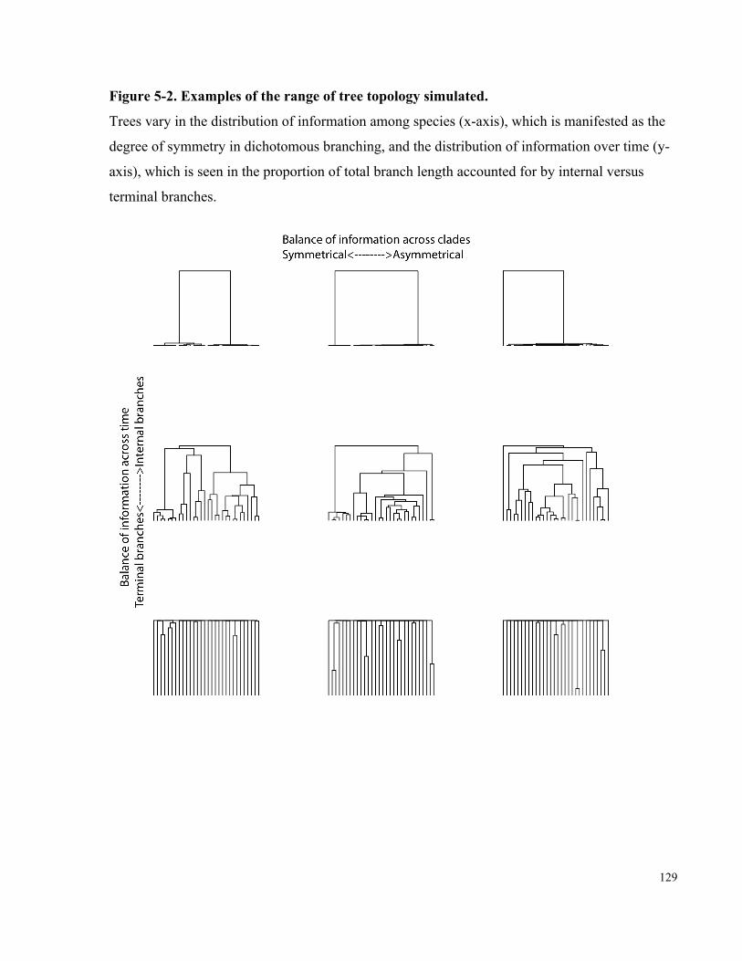
129
Figure 5-2. Examples of the range of tree topology simulated.
Trees vary in the distribution of information among species (x-axis), which is manifested as the
degree of symmetry in dichotomous branching, and the distribution of information over time (y-
axis), which is seen in the proportion of total branch length accounted for by internal versus
terminal branches.

130
Figure 5-3. Spearman’s correlation (r) between species richness (SR) and phylogenetic
diversity (PD) as a function of tree topology.

131
Figure 5-4. A) Spearman’s correlation (r) between biogeographically-weighted species
richness (BSR) and biogeographically-weighted evolutionary distinctivness (BED), as a
function of tree topology and species range sizes. B) Spearman’s correlation (r) between
phylogenetic diversity (PD) and biogeographically-weighted evolutionary distinctivness
(BED), as a function of tree topology and species range sizes.
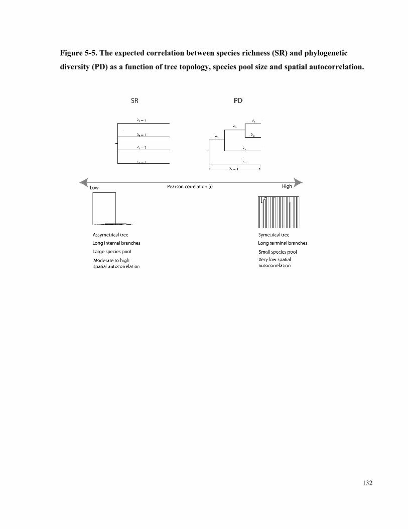
132
Figure 5-5. The expected correlation between species richness (SR) and phylogenetic
diversity (PD) as a function of tree topology, species pool size and spatial autocorrelation.
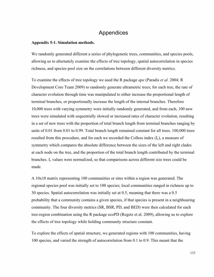
133
Appendices
Appendix 5-1. Simulation methods.
We randomly generated different a series of phylogenetic trees, communities, and species pools,
allowing us to alternately examine the effects of tree topology, spatial autocorrelation in species
richness, and species pool size on the correlations between different diversity metrics.
To examine the effects of tree topology we used the R package ape (Paradis et al. 2004; R
Development Core Team 2009) to randomly generate ultrametric trees; for each tree, the rate of
character evolution through time was manipulated to either increase the proportional length of
terminal branches, or proportionally increase the length of the internal branches. Therefore
10,000 trees with varying symmetry were initially randomly generated, and from each, 100 new
trees were simulated with sequentially slowed or increased rates of character evolution, resulting
in a set of new trees with the proportion of total branch length from terminal branches ranging by
units of 0.01 from 0.01 to 0.99. Total branch length remained constant for all trees. 100,000 trees
resulted from this procedure, and for each we recorded the Colless index (Ic), a measure of
symmetry which compares the absolute difference between the sizes of the left and right clades
at each node on the tree, and the proportion of the total branch length contributed by the terminal
branches. Ic values were normalized, so that comparisons across different size trees could be
made.
A 10x10 matrix representing 100 communities or sites within a region was generated. The
regional species pool was initially set to 100 species; local communities ranged in richness up to
30 species. Spatial autocorrelation was initially set at 0.5, meaning that there was a 0.5
probability that a community contains a given species, if that species is present in a neighbouring
community. The four diversity metrics (SR, BSR, PD, and BED) were then calculated for each
tree-region combination using the R package ecoPD (Regetz et al. 2009), allowing us to explore
the effects of tree topology while holding community structure constant.
To explore the effects of spatial structure, we generated regions with 100 communities, having
100 species, and varied the strength of autocorrelation from 0.1 to 0.9. This meant that the
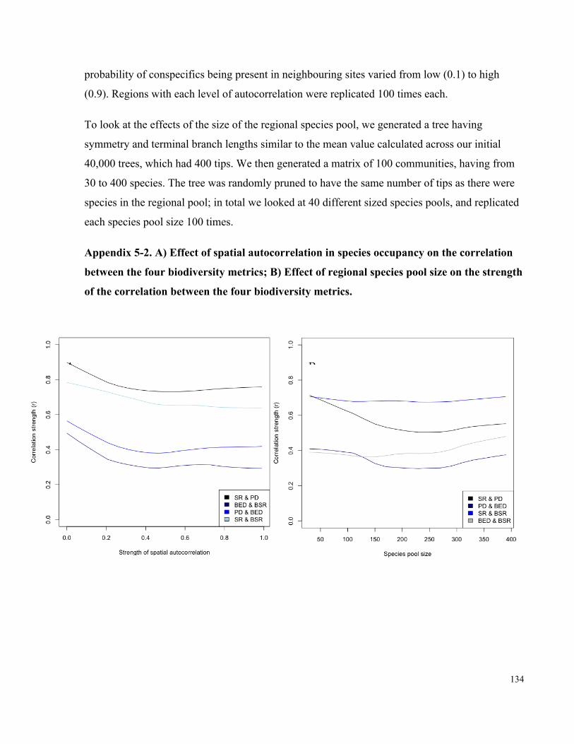
134
probability of conspecifics being present in neighbouring sites varied from low (0.1) to high
(0.9). Regions with each level of autocorrelation were replicated 100 times each.
To look at the effects of the size of the regional species pool, we generated a tree having
symmetry and terminal branch lengths similar to the mean value calculated across our initial
40,000 trees, which had 400 tips. We then generated a matrix of 100 communities, having from
30 to 400 species. The tree was randomly pruned to have the same number of tips as there were
species in the regional pool; in total we looked at 40 different sized species pools, and replicated
each species pool size 100 times.
Appendix 5-2. A) Effect of spatial autocorrelation in species occupancy on the correlation
between the four biodiversity metrics; B) Effect of regional species pool size on the strength
of the correlation between the four biodiversity metrics.
A B

135
Copyright Acknowledgements
Tucker, C.M. and Cadotte, M.W. 2013. Unifying measures of biodiversity: understanding when
richness and phylogenetic diversity should be congruent. Diversity and Distributions. DOI:
10.1111/ddi.12087.
Copyright © 1999–2013 John Wiley & Sons, Inc. All Rights Reserved.

136
Conclusions: Accounting for diversity in a changing world
Understanding global biodiversity—both the mechanisms that promote and maintain diversity
and the contribution of diversity to ecosystem services—informs management and conservation
in vital ways. Habitat loss, climate change, and species invasions all contribute to high rates of
contemporary species extinctions, and combining ecological theory, particularly with a focus on
mechanisms, with ecological applications is necessary to successfully support conservation
activities. The ecological literature is replete with mechanisms through which species
coexistence can be allowed (and thus species diversity promoted). Reconciling these mechanisms
with the possible effects of changing climate and human actions on their efficacy is necessary
and still incomplete. For example, global warming will lead to changes in both the mean
temperature and precipitation, and possible effects on species extinctions, range shifts, invasion
success, and biome shifts have been explored (Stachowicz et al. 2002; Thomas et al. 2004;
Thomas et al. 2006; Colwell et al. 2008; Chen et al. 2011). Temperature and precipitation
extremes and overall variability will also change with warming, and the implications of changes
in variability regimes have received less attention, although ecological theory suggests that
environmental variability is also an important driver of species coexistence (Warner & Chesson
1985).
In this thesis, I provided theoretical and experimental evidence that environmental heterogeneity
affects species coexistence directly and also indirectly through its effects on other coexistence
mechanisms. Further, I suggested particular conservation and management actions that would be
improved if environmental heterogeneity were considered during planning. In addition, I
provided evidence that, regardless of the mechanisms producing and maintaining spatial patterns
of species, phylogenetic, or functional diversity, they tend to be spatially variable in their
distributions creating a need to explicitly prioritize diversity conservation and reserve selection.
Themes found throughout this thesis include the use of ecological theory to inform conservation,
broadening conservation activities to include multiple types of diversity, and recognizing the role
for environmental variability.
In the first three chapters, I explored the question of how environmental heterogeneity alters
expectations for species coexistence, mechanisms of diversity maintenance, and management
137
activities. In the first chapter, “Environmental Variability Counteracts Priority Effects to
Facilitate Species Coexistence: Evidence from Nectar Microbes”, I manipulated communities
of nectar bacteria and yeast species to explore whether temperature variability through space and
time altered the assembly of nectar microbe communities. Because nectar-dwelling communities
typically experience temperature variability through space and time, I hypothesized that
commonly-studied assembly mechanisms such as arrival order might interact with temperature
variability. A fully crossed design of temperature variability treatments (spatial, temporal, or
spatiotemporal) and arrival order (yeast first, bacteria first, or concurrent arrival) indicated that
variability and arrival order interacted to determine the end state of the community. In particular,
models suggested that temporal variability in temperature decreases the strength of priority effect
mechanisms such as habitat modification and resource consumption. Temporal variability in
temperature gave an advantage to temperature-tolerant bacterial species, such that they were
more likely to be present in communities that assembled in temporally variable conditions.
Ultimately these results provide a reminder that community assembly is a complex process
affected by multiple mechanisms. Studying only a single mechanism in isolation will limit our
ability to extend results to the complexities of real communities. Indeed, a key limitation of
laboratory microcosms is that they simplify the wide range of conditions likely to be important in
natural systems (Carpenter 1996; but see Srivastava et al. 2004). If a study of two mechanisms
(priority effects and temperature variability) alters expectations for community assembly, the
natural systems may not be easily understood from simplistic studies.
Annual plant species partition seasonal environmental variation to minimize competitive
interactions, leading to successional patterns of flowering and reproduction. Temperature cues
underlie most such phenological displays, and so the link between temperature and phenology is
used to track changes in global climate. However, observational data suggest that advances in
flowering time are highly variable. In “Community-level Interactions Alter Species’
Responses to Climate Change”, I used simple models of plant development to show that
mismatches between temperature regime and species’ optimal flowering temperatures occur with
warming, but competitive interactions can constrain species from closely tracking changes in
climate. Understanding the mechanisms by which species partitioning seasonal variation in
temperature here informs models of the effects of climate change on plant communities. This

138
model provides a template for one mechanism by which competition could introduce variation
into observations of flowering time. However, this is only one pathway by which biotic
interactions could interact with warming temperatures. Facilitative interactions or mutualisms
(e.g. pollinators) could introduce constraints on phenological shifts that counteract those driven
by competition, for example. Natural communities include both annual and perennial species,
and perennial species’ fitnesses and flowering times depend on conditions occurring in more than
a single year.
In “Fire Variability, as well as Frequency, can Explain Coexistence Between Seeder and
Resprouter Life Histories”, I connected ecological theory–coexistence driven by variability in
fire occurrences—with management considerations–the timing and nature of managed fire
regimes that is optimal for diversity maintenance. Recent evidence from Australian shrublands
suggests that modern invariant fire regimes are associated with declines in diversity. Where
species have long histories of adaptation to particular disturbance regimes (such as fire regimes
in Mediterranean hotspots), changes away from natural regimes could disrupt mechanisms of
coexistence. Model results enforced this line of thought: a disturbance-mediated storage effect
could explain the coexistence of competitively unequal shrubs in Mediterranean shrublands,
however this mechanism required that fire events vary in occurrence. Too high or too low
variability and diversity would decline. This suggested that fire management activities that
ignore variability in fire events miss an important component of diversity maintenance. To
determine if this general model has relevance for more specific shrub communities, it will still be
necessary to parameterize the model for specific shrub species and fire regimes. Observational
data from regions that have received differing fire regimes can also provide insight into the
importance of variability in fire occurrence.
The final two chapters provide observational and theoretical evidence that the spatial distribution
of different forms of biodiversity tend to be incongruent and this creates a need to explicitly
consider and prioritize each type of diversity in conservation activities. Researchers have argued
since the 1990s (Faith 1992; UN 1992) that all forms of diversity, not just species richness, have
intrinsic and extrinsic value, but most reserve-selection exercises and applications are species-
focused or habitat-focused. One outcome of this is that other forms of diversity such as a region’s
evolutionary history are not well protected. This proved true in the Cape Floristic Region of

139
South Africa, for which I showed in “Incorporating Geographical and Evolutionary Rarity
into Conservation Prioritization” that although Proteaceae species are well protected by
existing international, national, provincial, and regional protected areas, phylogenetic diversity
and range-restricted evolutionary distinctiveness is poorly protected. This proved true regardless
of the degree of resolution of the Proteaceae phylogeny. While showing that alternate forms of
diversity are not captured by extant reserves is an important first step, ultimately political and
economic limitations will determine where future reserves are placed in the Cape Floristic
Region.
The spatial divergence of different forms of diversity can provide insight into the ecological and
evolutionary processes structuring communities as well as informing diversity prioritization. It
places increased pressure on managers however, to obtain and understand information about
multiple types of diversity. Surveys of species richness, for example, tend to be more often
available than evolutionary history, and more easily interpreted. In the final chapter, “Unifying
measures of biodiversity: understanding when richness and phylogenetic diversity should
be congruent”, I provide some insight into this problem by demonstrating that the spatial
congruence between measures such as species richness and phylogenetic diversity is predictably
related to evolutionary history and spatial extent of species’ ranges. When species are anciently
diverged, there are relatively few species, or species ranges are large and disjoint, phylogenetic
diversity and species richness tend to agree, suggesting that a “one-size fits all” conservation
plan will be effective. However, in many biodiversity hotspots, diversification rates vary through
time, species pools are large (hence the initial desire to protect the region) and species are often
range-limited or endemic. In these situations, explicitly considering multiple forms of diversity
separately may be necessary.
The findings presented in this thesis attempt to connect ecological theory with applications for
management and conservation. Ecology has the duty to integrate ecological knowledge and
theory with real-world applications, and it can at times be difficult to understand and express the
connections between highly generalized theory and highly specific real world problems. When
the connections depend on models and/or highly controlled laboratory experiments (as they do in
Chapters 1, 2, 3 & 5), it is likely that experimental work in the field and tests of observation data
will be necessary to test whether the suggested mechanisms tend to be important in natural

140
systems and whether they are altered by interactions with other mechanisms. However, models
of constraints on phenological shifts or coexistence promoted by fire variability provide clearly
testable hypotheses and as such play an important role in combining theory and application.
Future directions require both that we understand how theory applies to natural ecosystems, and
further than relevant knowledge is transferred to managers and policy makers so that it can be
meaningfully applied in the real world.

141
References
Carpenter S.R. (1996). Microcosm experiments have limited relevance for community and ecosystem ecology. Ecology, 77, 677-680.
Chen I.-C., Hill J.K., Ohlemoller R., Roy D.B. & Thomas C.D. (2011). Rapid range shifts of species associated with high levels of climate warming. Science, 333, 1024-1026.
Colwell R.K., Brehm G., Cardelis C.L., Gilman A.C. & Longino J.T. (2008). Global warming, elevational range shifts, and lowland biotic attrition in the wet tropics. Science, 322, 258-261.
Faith D.P. (1992). Conservation evaluation and phylogenetic diversity. Biological Conservation, 61, 1-10.
Srivastava D.S., Kolasa J., Bengtsson J., Gonzalez A., Lawler S.P., Miller T.E., Munguia P., Romanuk T., Schneider D.C. & Trzcinski M.K. (2004). Are natural microcosms useful model systems for ecology? Trends in Ecology & Evolution, 19, 379-384.
Stachowicz J.J., Terwin J.R., Whitlatch R.B. & Osman R.W. (2002). Linking climate change and biological invasions: ocean warming facilitates nonindigenous species invasions. Proceedings of the National Academy of Sciences, 99, 15497-15500.
Thomas C.D., Cameron A., Green R.E., Bakkenes M., Beaumont L.J., Collingham Y.C., Erasmus B.F., De Siqueira M.F., Grainger A. & Hannah L. (2004). Extinction risk from climate change. Nature, 427, 145-148.
Thomas C.D., Franco A. & Hill J.K. (2006). Range retractions and extinction in the face of climate warming. Trends in Ecology & Evolution, 21, 415-416.
United Nations (1992). Convention on Biological Diversity.
Warner R.R. & Chesson P. (1985). Coexistence mediated by recruitment fluctuations: a field guide to the storage effect. The American Naturalist, 125, 769-787.