bio-inspired algorithms for fuzzy rule-based systems · bio-inspired algorithms for fuzzy...

TMRF e-Book Advanced Knowledge Based Systems: Model, Applications & Research (Eds. Sajja & Akerkar), Vol. 1, pp 126 – 159, 2010 Chapter 7

Bio-Inspired Algorithms for Fuzzy Rule-Based Systems Bahareh Atoufi * and Hamed Shah-Hosseini † Abstract In this chapter we focus on three bio-inspired algorithms and their combinations with fuzzy rule based systems. Rule Based systems are widely being used in decision making, control systems and forecasting. In the real world, much of the knowledge is imprecise and ambiguous but fuzzy logic provides for systems better presentations of the knowledge, which is often expressed in terms of the natural language. Fuzzy rule based systems constitute an extension of classical Rule-Based Systems, because they deal with fuzzy rules instead of classical logic rules. Since bio-inspired optimization algorithms have been shown effective in improving the tuning the parameters and learning the Fuzzy Rule Base, our major objective is to represent the application of these algorithms in improving the Knowledge Based Systems with focus on Rule-Base Learning. We first introduce the Evolutionary Computation and Swarm Intelligence topics as a subfield of Computational Intelligence dealing with Combinatorial Optimization problems. Then, three following bio-inspired algorithms, i.e. Genetic Algorithms, Ant Colony Optimization, and Particle Swarm Optimization are explained and their application in improving the knowledge Based Systems are presented. INTRODUCTION The generation of the Knowledge Base (KB) of a Fuzzy Rule-Based System (FRBS) [Mamdani E.H., 1982] presents several difficulties because the KB depends on the concrete application, and this makes the accuracy of the FRBS directly depend on its composition. Many approaches have been proposed to automatically learn the KB from numerical information. Most of them have focused on the Rule Base (RB) learning, using a predefined Data Base (DB) [Cordón et al. 1998]. This operation mode makes the DB have a significant influence on the FRBS performance. In fact, some studies have shown that the system performance is much more sensitive to the choice of the semantics in the DB than to the composition of the RB. The usual solution for improving the FRBS performance in dealing with the DB components involves a tuning process of the preliminary DB definition once the RB has been derived. This process only adjusts the membership function definitions and does not modify the

* Department of Electrical and Computer Engineering, Shahid Beheshti University, G.C., [email protected] † Corresponding author: Department of Electrical and Computer Engineering, Shahid Beheshti University, G.C., [email protected], [email protected]

Bio-inspired Algorithms for Fuzzy Rule Based Systems

127

number of linguistic terms in each fuzzy partition since the RB remains unchanged. In contrast to this, a posteriori DB learning, there are some approaches that learn the different DB components a priori. The objective of this chapter is to introduce methods to automatically generate the KB of an FRBS based on learning approach. We show the application of Evolutionary Computation (EC) [ Back T., Schwefel H.P. 1986] and Swarm Intelligence (Genetic Algorithms (GA) [Goldberg D.E., 1989], Ant Colony Optimization (ACO) [Dorigo M., 1992], and Particle Swarm Optimization (PSO)[Kennedy J., Eberhart R.C. 1995] ) in improving the Rule-base learning. The outline of the chapter is as follows: in Section 1, we introduce the Evolutionary Computing concept. In addition to a brief history, we give an introduction to some of the biological processes that have served as an inspiration and that have provided rich sources of ideas and metaphors to researchers. The GA as part of EC is described in a subsection of this part. In Section 2, Swarm Intelligence is described with focus on introducing ACO and PSO as the most popular optimization algorithms based on Swarm Intelligence used for fuzzy rule bases. Section 3 includes an introduction to Fuzzy Rule-Based Systems as an extension of classical Rule-Based systems. Genetic Fuzzy Rule-Based Systems are introduced in Section 4. Generating the Knowledge Base of a Fuzzy Rule-Based System by the Genetic Learning of the Data Base is discussed here. In this part, we give the reader an idea about Genetic Tuning and Genetic Learning of Rule Bases. Section 5 is devoted to introduce all the aspects related to ACO algorithms specialized to the FRL (Fuzzy Rule Learning) problem. Here, the learning task is formulated as an optimization problem and is solved by the ACO. Finally, in Section 6, application of PSO for Fuzzy Rule-Based System is discussed. 1. EVOLUTIONARY COMPUTATION Nearly three decades of research and applications have clearly demonstrated that the mimicked search process of natural evolution can yield very robust, direct computer algorithms, although these imitations are crude simplifications of biological reality. The resulting Evolutionary Algorithms are based on the collective learning process within a population of individuals, each of which represents a search point in the space of potential solutions to a given problem. The population is arbitrarily initialized, and it evolves towards better and better regions of the search space by means of randomized processes of selection (which is deterministic in some algorithms), mutation, and recombination (which is completely omitted in some algorithmic realizations). The environment (given aim of the search) delivers some information about quality (fitness value) of the search points, and the selection process favors those individuals of higher fitness to reproduce more often than worse individuals. The recombination mechanism allows the mixing of parental information while passing it to their descendants, and mutation introduces innovation into the population.

RRf n →: denotes the objective function to be optimized, and without loss of generality we assume a minimization task in the following. In general, fitness and objective function values of an individual are not required to be identical, such that fitness RI →Φ : (I being the space of individuals) and f are distinguished mappings (but f is always a component of Φ ). While Ia ∈

r is

used to denote an individual, nRx ∈r

indicates an object variable vector. Furthermore 1≤μ denotes the size of the parent population and 1≥λ is the offspring population size, i.e. the number of individuals created by means of recombination and mutation at each generation (if the life time of individuals is limited to one generation, i.e. selection is not elitist, μλ ≥ is a more reasonable

assumption). A population at generation t, )}(),...,({)( 1 tatatP μrr

= consists of individuals,

Itai ∈)(r , and λμ IIrr

→Θ : denotes the recombination operator which might be controlled by

Advanced Knowledge Based Systems: Models, Applications & Research

128

128

additional parameters summarized in the set rΘ .Similarly, the mutation operator λλ IImm

→Θ :

modifies the offspring population, again being controlled by some parameters mΘ . Both mutation and recombination, though introduced here as macro-operators transforming populations into populations, can essentially be reduced to local operators IIm

m→′Θ : and IIr

r→′Θ

μ: that create one individual when applied. These local variants will be used when the particular instances of the operators are explained in subsequent Sections. Selection μλμλ IIIs

s→∪ +

Θ )(: is applied to choose the parent population of the next generation. During the evaluation steps the fitness function

RI →Φ : is calculated for all individuals of a population, and },{: falsetrueI →μι is used to denote the termination criterion. The resulting algorithmic description is given below.

Here, )}(,0{ tPQ ∈ is a set of individuals that are additionally taken into account during the selection step. The evaluation process yields a multi-set of fitness values, which in general are not necessarily identical to objective function values. However, since the selection criterion operates on fitness instead of objective function values, fitness values are used here as result of the evaluation process. During the calculation of fitness, the evaluation of objective function values is always necessary, such that the information is available and can easily be stored in an appropriate data structure. Three main streams of instances of this general algorithm, developed independently of each other, can nowadays be identified: Evolutionary Programming (EP), originally developed by L. J. Fogel, A. J. Owens, and M. J.Walsh in the U.S., Evolution Strategies (ESs), developed in Germany by I. Rechenberg, and Genetic Algorithms (GAs) by J. Holland in the U.S. as well, with refinements by D. Goldberg. Each of these main stream algorithms have clearly demonstrated their capability to yield good approximate solutions even in case of complicated multimodal, discontinuous, non-differentiable, and even noisy or moving response surfaces of optimization problems. Within each research community, parameter optimization has been a common and highly successful theme of applications. Evolutionary Programming and especially GAs, however, were designed with a very much broader range of possible applications in mind and confirmed their wide applicability by a variety of important examples in fields like machine learning, control, automatic programming, planning, and etc. Here, we focus on GA as a successful optimization method which has been shown effective in improving the tuning the parameters and learning the Fuzzy Rule Base.


129

1.1 Genetic Algorithm GA is a part of evolutionary computing. In fact, they are adaptive heuristic search algorithms premised on the evolutionary ideas of natural selection and genetic. The basic concept of GA is designed to simulate processes in the natural system necessary for evolution, specifically as you can guess, GAs often follow the principles first laid down by Charles Darwin of survival of the fittest. As such they represent an intelligent exploitation of a random search within a defined search space to solve a problem. First pioneered by John Holland in the 60s, GA has been widely studied, experimented and applied in many fields in engineering worlds. Not only does GA provide an alternative method to problem solving, it consistently outperforms other traditional methods in most of the problems. Many of the real world problems involved finding optimal parameters, which might prove difficult for traditional methods but ideal for GA. However, because of its outstanding performance in optimization, GA has been regarded as a function optimizer. In fact, there are many ways to view GA. Perhaps, most users come to GA, looking for a problem solver, but this is a restrictive view. In fact, GA can be examined as a number of different things:

• GA as problem solvers • GA as challenging technical puzzle • GA as basis for competent machine learning • GA as computational model of innovation and creativity • GA as computational model of other innovating systems • GA as guiding philosophy

However, due to various constraints, we would only be looking at GAs as problem solvers here. The problem addressed by GA is to search a space of candidate hypotheses to identify the best hypothesis. In GA, the "best hypothesis" is defined as the one that optimizes a predefined numerical measure for the problem at hand, called the hypothesis fitness. Although different implementations of GA vary in their details, they typically share the following structure: The algorithm operates by iteratively updating a pool of hypotheses, called the population. In each iteration, all members of the population are evaluated according to the fitness function. A new population is then generated by probabilistically selecting the fittest individuals from the current population. Some of these selected individuals are carried forward into the next generation population intact. Others are used as the basis for creating new offspring individuals by applying genetic operations such as crossover and mutation. A prototypical GA is described in Table 1.1 The input to this algorithm includes the fitness function for ranking candidate hypotheses, a threshold defining an acceptable level of fitness for terminating the algorithm, the size of the population to be maintained, and parameters that determine how successor populations are to be generated: the fraction of the population to be replaced at each generation and the mutation rate. Notice in this algorithm each iteration through the main loop produces a new generation of hypotheses based on the current population.


130

130

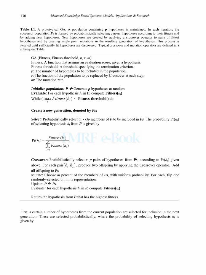
Table 1.1. A prototypical GA. A population containing p hypotheses is maintained. In each iteration, the successor population Ps is formed by probabilistically selecting current hypotheses according to their fitness and by adding new hypotheses. New hypotheses are created by applying a crossover operator to pairs of fittest hypotheses and by creating single point mutations in the resulting generation of hypotheses. This process is iterated until sufficiently fit hypotheses are discovered. Typical crossover and mutation operators are defined in a subsequent Table.

GA (Fitness, Fitness-threshold, p, r, m) Fitness: A function that assigns an evaluation score, given a hypothesis. Fitness-threshold: A threshold specifying the termination criterion. p: The number of hypotheses to be included in the population. r: The fraction of the population to be replaced by Crossover at each step. m: The mutation rate. Initialize population: P Generate p hypotheses at random Evaluate: For each hypothesis hi in P, compute Fitness(hi) While ( )(max ii

hFitness < Fitness-threshold ) do

Create a new generation, denoted by Ps: Select: Probabilistically select (1 - r)p members of P to be included in Ps. The probability Pr(hi) of selecting hypothesis hi from P is given by

∑=

= P

ji

ii

hFitness

hFitnessh

1)(

)()Pr(

Crossover: Probabilistically select r⋅ p pairs of hypotheses from Ps, according to Pr(hi) given above. For each pair ],[ 21 hh , produce two offspring by applying the Crossover operator. Add all offspring to Ps Mutate: Choose m percent of the members of Ps, with uniform probability. For each, flip one randomly-selected bit in its representation. Update: P Ps Evaluate: for each hypothesis hi in P, compute Fitness(hi) Return the hypothesis from P that has the highest fitness.

First, a certain number of hypotheses from the current population are selected for inclusion in the next generation. These are selected probabilistically, where the probability of selecting hypothesis hi is given by


131

∑=

= P

ji

ii

hFitness

hFitnessh

1)(

)()Pr( (1)

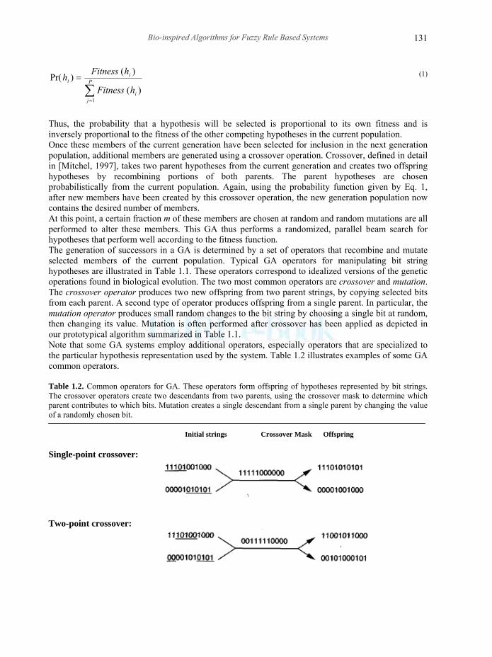
Thus, the probability that a hypothesis will be selected is proportional to its own fitness and is inversely proportional to the fitness of the other competing hypotheses in the current population. Once these members of the current generation have been selected for inclusion in the next generation population, additional members are generated using a crossover operation. Crossover, defined in detail in [Mitchel, 1997], takes two parent hypotheses from the current generation and creates two offspring hypotheses by recombining portions of both parents. The parent hypotheses are chosen probabilistically from the current population. Again, using the probability function given by Eq. 1, after new members have been created by this crossover operation, the new generation population now contains the desired number of members. At this point, a certain fraction m of these members are chosen at random and random mutations are all performed to alter these members. This GA thus performs a randomized, parallel beam search for hypotheses that perform well according to the fitness function. The generation of successors in a GA is determined by a set of operators that recombine and mutate selected members of the current population. Typical GA operators for manipulating bit string hypotheses are illustrated in Table 1.1. These operators correspond to idealized versions of the genetic operations found in biological evolution. The two most common operators are crossover and mutation. The crossover operator produces two new offspring from two parent strings, by copying selected bits from each parent. A second type of operator produces offspring from a single parent. In particular, the mutation operator produces small random changes to the bit string by choosing a single bit at random, then changing its value. Mutation is often performed after crossover has been applied as depicted in our prototypical algorithm summarized in Table 1.1. Note that some GA systems employ additional operators, especially operators that are specialized to the particular hypothesis representation used by the system. Table 1.2 illustrates examples of some GA common operators. Table 1.2. Common operators for GA. These operators form offspring of hypotheses represented by bit strings. The crossover operators create two descendants from two parents, using the crossover mask to determine which parent contributes to which bits. Mutation creates a single descendant from a single parent by changing the value of a randomly chosen bit. Initial strings Crossover Mask Offspring Single-point crossover:

Two-point crossover:


132

132

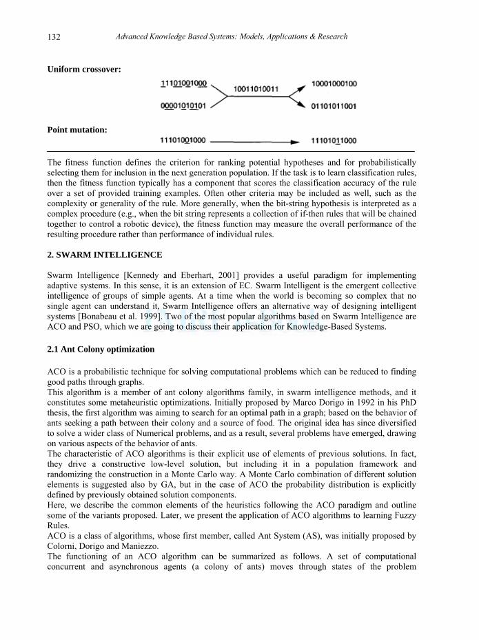
Uniform crossover:

Point mutation: The fitness function defines the criterion for ranking potential hypotheses and for probabilistically selecting them for inclusion in the next generation population. If the task is to learn classification rules, then the fitness function typically has a component that scores the classification accuracy of the rule over a set of provided training examples. Often other criteria may be included as well, such as the complexity or generality of the rule. More generally, when the bit-string hypothesis is interpreted as a complex procedure (e.g., when the bit string represents a collection of if-then rules that will be chained together to control a robotic device), the fitness function may measure the overall performance of the resulting procedure rather than performance of individual rules. 2. SWARM INTELLIGENCE Swarm Intelligence [Kennedy and Eberhart, 2001] provides a useful paradigm for implementing adaptive systems. In this sense, it is an extension of EC. Swarm Intelligent is the emergent collective intelligence of groups of simple agents. At a time when the world is becoming so complex that no single agent can understand it, Swarm Intelligence offers an alternative way of designing intelligent systems [Bonabeau et al. 1999]. Two of the most popular algorithms based on Swarm Intelligence are ACO and PSO, which we are going to discuss their application for Knowledge-Based Systems. 2.1 Ant Colony optimization ACO is a probabilistic technique for solving computational problems which can be reduced to finding good paths through graphs. This algorithm is a member of ant colony algorithms family, in swarm intelligence methods, and it constitutes some metaheuristic optimizations. Initially proposed by Marco Dorigo in 1992 in his PhD thesis, the first algorithm was aiming to search for an optimal path in a graph; based on the behavior of ants seeking a path between their colony and a source of food. The original idea has since diversified to solve a wider class of Numerical problems, and as a result, several problems have emerged, drawing on various aspects of the behavior of ants. The characteristic of ACO algorithms is their explicit use of elements of previous solutions. In fact, they drive a constructive low-level solution, but including it in a population framework and randomizing the construction in a Monte Carlo way. A Monte Carlo combination of different solution elements is suggested also by GA, but in the case of ACO the probability distribution is explicitly defined by previously obtained solution components. Here, we describe the common elements of the heuristics following the ACO paradigm and outline some of the variants proposed. Later, we present the application of ACO algorithms to learning Fuzzy Rules. ACO is a class of algorithms, whose first member, called Ant System (AS), was initially proposed by Colorni, Dorigo and Maniezzo. The functioning of an ACO algorithm can be summarized as follows. A set of computational concurrent and asynchronous agents (a colony of ants) moves through states of the problem


133

corresponding to partial solutions of the problem to solve. They move by applying a stochastic local decision policy based on two parameters, called trails and attractiveness. By moving, each ant incrementally constructs a solution to the problem. When an ant completes a solution, or during the construction phase, the ant evaluates the solution and modifies the pheromone trail value on the components used in its solution. This pheromone information will direct the search of the future ants. Furthermore, an ACO algorithm includes two more mechanisms: trail evaporation and, optionally, daemon actions. Trail evaporation decreases all trail values over time, in order to avoid unlimited accumulation of trails over some component. Daemon actions can be used to implement centralized actions which cannot be performed by single ants, such as the invocation of a local optimization procedure, or the update of global information to be used to decide whether to bias the search process from a non-local perspective. More specifically, an ant is a simple computational agent, which iteratively constructs a solution for the instance to solve. Partial problem solutions are seen as states. At the core of the ACO algorithm lies a loop, where at each iteration, each ant moves (performs a step) from a state ι to another one ψ, corresponding to a more complete partial solution. That is, at each step, each ant k computes a set

( )ισkA of feasible expansions to its current state, and moves to one of these in probability. The

probability distribution is specified as follows. For ant k, the probability kpιψ of moving from state ι to

state ψ depends on the combination of two values:

the attractiveness ιψη of the move, as computed by some heuristic indicating the a priori desirability of

that move‡;

the pheromone trail level ιψτ of the move, indicating how efficient it has been in the past to make that particular move: it represents therefore an a posteriori indication of the desirability of that move. Trails are updated usually when all ants have completed their solution, increasing or decreasing the level of trails corresponding to moves that were part of "good" or "bad" solutions, respectively. The importance of the original Ant System (AS) resides mainly in being the prototype of a number of ant algorithms, which collectively implement the ACO paradigm. The components of AS are specifies as follows. The move probability distribution defines probabilities kpιψ to be equal to 0 for all moves which are infeasible (i.e., they are in the tabu list of ant k, that is a list containing all moves which are infeasible for ants k starting from state ι, otherwise they are computed by means of Eq. 2, where α and β are user defined parameters (another parameter, 10 ≤≤ ρ ):

‡ The attractiveness of a move can be effectively estimated by means of lower bounds (upper bounds in the case of maximization problems) on the cost of the completion of a partial solution. In fact, if a state ι corresponds to a partial problem solution it is possible to compute a lower bound on the cost of a complete solution containing ι. Therefore, for each feasible move ι,ψ, it is possible to compute the lower bound on the cost of a complete solution containing ψ: the lower the bound the better the move.


134

134

( )⎪⎩

⎪⎨

⎧

×

×

= ∑ ∉

0ktabu

kp ζβ

ιζαιζ

βιψ

αιψ

ιψ ητητ

ktabuif ∉)(ιψ (2)

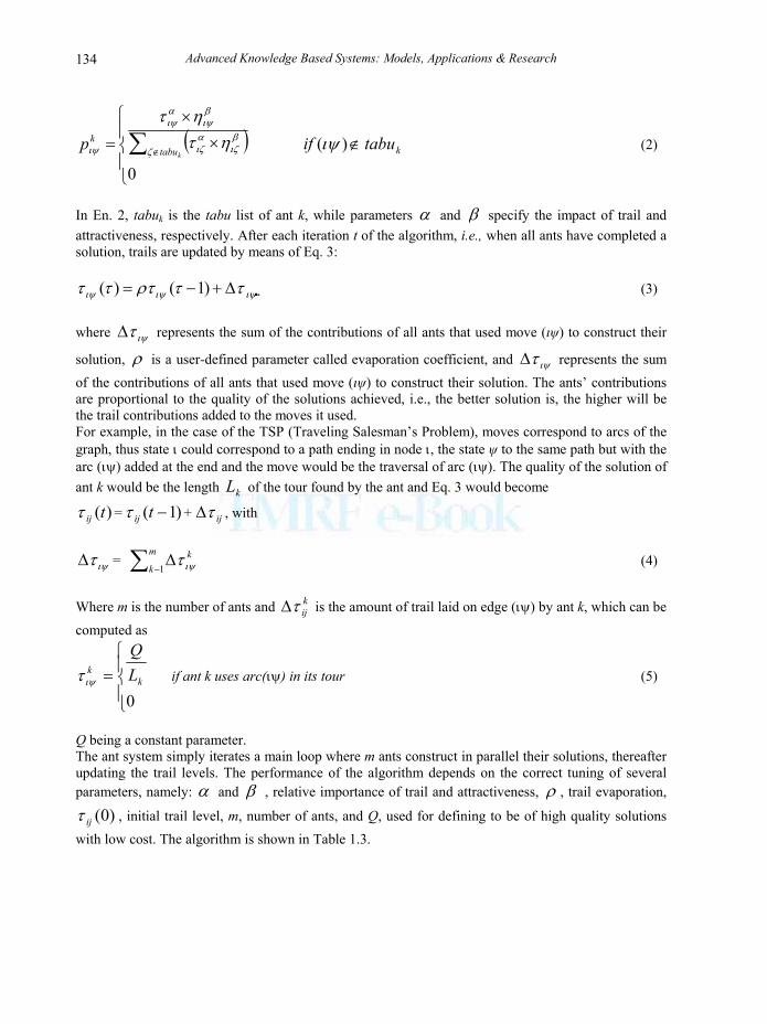
In En. 2, tabuk is the tabu list of ant k, while parameters α and β specify the impact of trail and attractiveness, respectively. After each iteration t of the algorithm, i.e., when all ants have completed a solution, trails are updated by means of Eq. 3:

ιψιψιψ ττρτττ Δ+−= )1()( (3) where ιψτΔ represents the sum of the contributions of all ants that used move (ιψ) to construct their

solution, ρ is a user-defined parameter called evaporation coefficient, and ιψτΔ represents the sum of the contributions of all ants that used move (ιψ) to construct their solution. The ants’ contributions are proportional to the quality of the solutions achieved, i.e., the better solution is, the higher will be the trail contributions added to the moves it used. For example, in the case of the TSP (Traveling Salesman’s Problem), moves correspond to arcs of the graph, thus state ι could correspond to a path ending in node ι, the state ψ to the same path but with the arc (ιψ) added at the end and the move would be the traversal of arc (ιψ). The quality of the solution of ant k would be the length kL of the tour found by the ant and Eq. 3 would become

)(tijτ = )1( −tijτ + ijτΔ , with

ιψτΔ = ∑ −Δ

m

kk

1 ιψτ (4)

Where m is the number of ants and k

ijτΔ is the amount of trail laid on edge (ιψ) by ant k, which can be computed as

⎪⎩

⎪⎨

⎧=

0k

k LQ

ιψτ if ant k uses arc(ιψ) in its tour (5)

Q being a constant parameter. The ant system simply iterates a main loop where m ants construct in parallel their solutions, thereafter updating the trail levels. The performance of the algorithm depends on the correct tuning of several parameters, namely: α and β , relative importance of trail and attractiveness, ρ , trail evaporation,

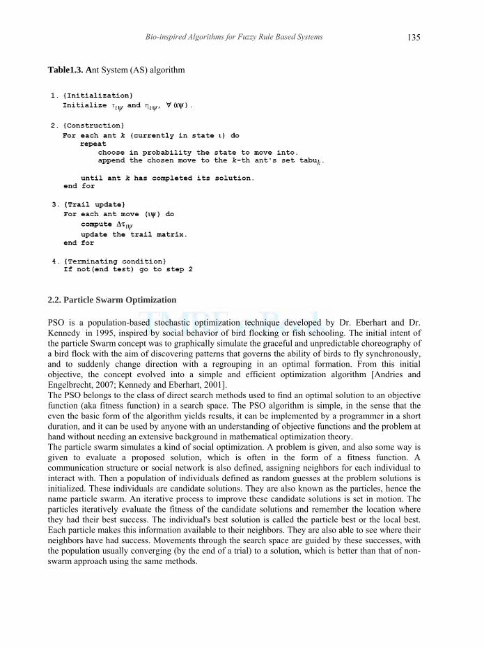
)0(ijτ , initial trail level, m, number of ants, and Q, used for defining to be of high quality solutions with low cost. The algorithm is shown in Table 1.3.


135

Table1.3. Ant System (AS) algorithm

2.2. Particle Swarm Optimization PSO is a population-based stochastic optimization technique developed by Dr. Eberhart and Dr. Kennedy in 1995, inspired by social behavior of bird flocking or fish schooling. The initial intent of the particle Swarm concept was to graphically simulate the graceful and unpredictable choreography of a bird flock with the aim of discovering patterns that governs the ability of birds to fly synchronously, and to suddenly change direction with a regrouping in an optimal formation. From this initial objective, the concept evolved into a simple and efficient optimization algorithm [Andries and Engelbrecht, 2007; Kennedy and Eberhart, 2001]. The PSO belongs to the class of direct search methods used to find an optimal solution to an objective function (aka fitness function) in a search space. The PSO algorithm is simple, in the sense that the even the basic form of the algorithm yields results, it can be implemented by a programmer in a short duration, and it can be used by anyone with an understanding of objective functions and the problem at hand without needing an extensive background in mathematical optimization theory. The particle swarm simulates a kind of social optimization. A problem is given, and also some way is given to evaluate a proposed solution, which is often in the form of a fitness function. A communication structure or social network is also defined, assigning neighbors for each individual to interact with. Then a population of individuals defined as random guesses at the problem solutions is initialized. These individuals are candidate solutions. They are also known as the particles, hence the name particle swarm. An iterative process to improve these candidate solutions is set in motion. The particles iteratively evaluate the fitness of the candidate solutions and remember the location where they had their best success. The individual's best solution is called the particle best or the local best. Each particle makes this information available to their neighbors. They are also able to see where their neighbors have had success. Movements through the search space are guided by these successes, with the population usually converging (by the end of a trial) to a solution, which is better than that of non-swarm approach using the same methods.


136

136

The swarm is typically modeled by particles in multidimensional space that have a position and a velocity. These particles fly through hyperspace (i.e. Rn) and have two essential reasoning capabilities: their memory of their own best position and knowledge of the global or their neighborhood's best. In a minimization optimization problem, problems are formulated so that "best" simply means the position with the smallest objective value. Members of a swarm communicate good positions to each other and adjust their own position and velocity based on these good positions. So a particle has the following information to make a suitable change in its position and velocity:

• A global best that is known to all and immediately updated when a new best position is found by any particle in the swarm.

• Neighborhood best that the particle obtains by communicating with a subset of the swarm. • The local best, which is the best solution that the particle has seen.

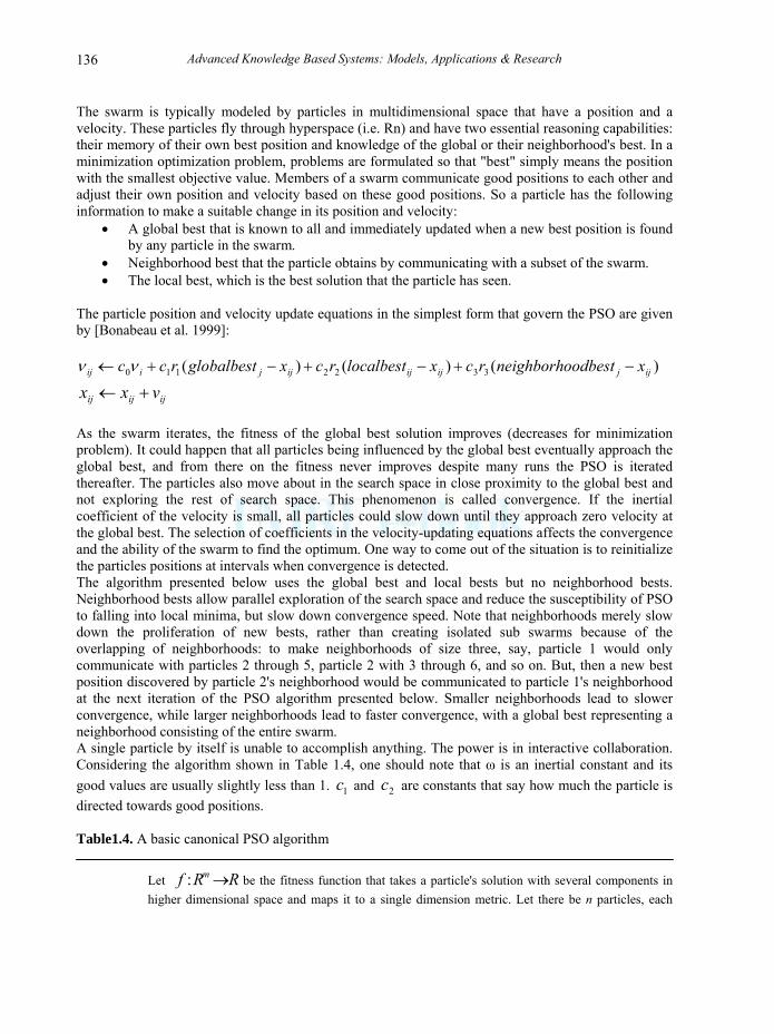
The particle position and velocity update equations in the simplest form that govern the PSO are given by [Bonabeau et al. 1999]:

)()()( 3322110 ijjijijijjiij xodbestneighborhorcxlocalbestrcxglobalbestrcc −+−+−+← νν

ijijij vxx +← As the swarm iterates, the fitness of the global best solution improves (decreases for minimization problem). It could happen that all particles being influenced by the global best eventually approach the global best, and from there on the fitness never improves despite many runs the PSO is iterated thereafter. The particles also move about in the search space in close proximity to the global best and not exploring the rest of search space. This phenomenon is called convergence. If the inertial coefficient of the velocity is small, all particles could slow down until they approach zero velocity at the global best. The selection of coefficients in the velocity-updating equations affects the convergence and the ability of the swarm to find the optimum. One way to come out of the situation is to reinitialize the particles positions at intervals when convergence is detected. The algorithm presented below uses the global best and local bests but no neighborhood bests. Neighborhood bests allow parallel exploration of the search space and reduce the susceptibility of PSO to falling into local minima, but slow down convergence speed. Note that neighborhoods merely slow down the proliferation of new bests, rather than creating isolated sub swarms because of the overlapping of neighborhoods: to make neighborhoods of size three, say, particle 1 would only communicate with particles 2 through 5, particle 2 with 3 through 6, and so on. But, then a new best position discovered by particle 2's neighborhood would be communicated to particle 1's neighborhood at the next iteration of the PSO algorithm presented below. Smaller neighborhoods lead to slower convergence, while larger neighborhoods lead to faster convergence, with a global best representing a neighborhood consisting of the entire swarm. A single particle by itself is unable to accomplish anything. The power is in interactive collaboration. Considering the algorithm shown in Table 1.4, one should note that ω is an inertial constant and its good values are usually slightly less than 1. 1c and 2c are constants that say how much the particle is directed towards good positions. Table1.4. A basic canonical PSO algorithm

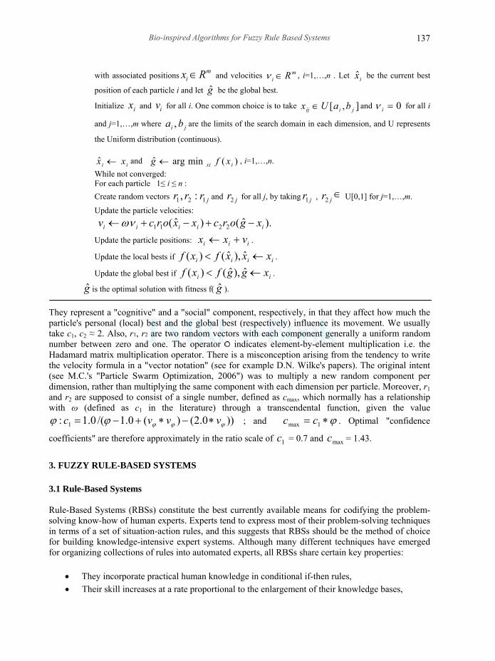
Let RRf m →: be the fitness function that takes a particle's solution with several components in higher dimensional space and maps it to a single dimension metric. Let there be n particles, each


137

with associated positions mi Rx ∈ and velocities m

i R∈ν , i=1,…,n . Let ix be the current best

position of each particle i and let g be the global best.

Initialize ix and iv for all i. One common choice is to take ],[ jiij baUx ∈ and 0=iν for all i

and j=1,…,m where ji ba , are the limits of the search domain in each dimension, and U represents

the Uniform distribution (continuous).

ix ix← and )(minargˆ ixi xfg ← , i=1,…,n. While not converged: For each particle 1≤ i ≤ n : Create random vectors jrrr 121 :, and jr2 for all j, by taking jr1 , jr2

∈ U[0,1] for j=1,…,m.

Update the particle velocities: ).ˆ()ˆ( 2211 iiiii xgorcxxorcv −+−+← ων

Update the particle positions: iii vxx +← .

Update the local bests if iiii xxxfxf ←< ˆ),ˆ()( .

Update the global best if ii xggfxf ←< ˆ),ˆ()( .

g is the optimal solution with fitness f( g ). They represent a "cognitive" and a "social" component, respectively, in that they affect how much the particle's personal (local) best and the global best (respectively) influence its movement. We usually take c1, c2 ≈ 2. Also, r1, r2 are two random vectors with each component generally a uniform random number between zero and one. The operator indicates element-by-element multiplication i.e. the Hadamard matrix multiplication operator. There is a misconception arising from the tendency to write the velocity formula in a "vector notation" (see for example D.N. Wilke's papers). The original intent (see M.C.'s "Particle Swarm Optimization, 2006") was to multiply a new random component per dimension, rather than multiplying the same component with each dimension per particle. Moreover, r1 and r2 are supposed to consist of a single number, defined as cmax, which normally has a relationship with ω (defined as c1 in the literature) through a transcendental function, given the value

))0.2()(0.1/(0.1: 1 ϕϕϕϕϕ vvvc ∗−∗+−= ; and ϕ∗= 1max cc . Optimal "confidence

coefficients" are therefore approximately in the ratio scale of 1c = 0.7 and maxc = 1.43.

3. FUZZY RULE-BASED SYSTEMS

3.1 Rule-Based Systems Rule-Based Systems (RBSs) constitute the best currently available means for codifying the problem-solving know-how of human experts. Experts tend to express most of their problem-solving techniques in terms of a set of situation-action rules, and this suggests that RBSs should be the method of choice for building knowledge-intensive expert systems. Although many different techniques have emerged for organizing collections of rules into automated experts, all RBSs share certain key properties:

• They incorporate practical human knowledge in conditional if-then rules, • Their skill increases at a rate proportional to the enlargement of their knowledge bases,


138

138

• They can solve a wide range of possibly complex problems by selecting relevant rules and then combining the results inappropriate ways,

• They adaptively determine the best sequence of rules to execute, and • They explain their conclusions by retracing their actual lines of reasoning and translating the

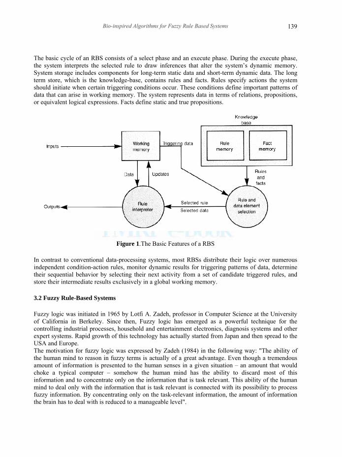
logic of each rule employed into natural language. RBSs address a need for capturing, representing, storing, distributing, reasoning about, and applying human knowledge electronically. They provide a practical means of building automated experts in application areas where job excellence requires consistent reasoning and practical experience. The hallmark of these systems is the way they represent knowledge about plausible inferences and preferred problem-solving tactics. Typically, both sorts of know-how are represented as conditional rules. Roughly speaking, an RBS consists of a knowledge base and an inference engine (Figure 1). The knowledge base contains rules and facts. Rules always express a conditional, with an antecedent and a consequent component. The interpretation of a rule is that if the antecedent can be satisfied the consequent can too. When the consequent defines an action, the effect of satisfying the antecedent is to schedule the action for execution. When the consequent defines a conclusion, the effect is to infer the conclusion. Because the behavior of all RBSs derives from this simple regimen, their rules will always specify the actual behavior of the system when particular problem-solving data are entered. In doing so, rules perform a variety of distinctive functions:

• They define a parallel decomposition of state transition behavior, thereby inducing a parallel decomposition of the overall system state that simplifies auditing and explanation. Every result can thus be traced to its antecedent data and intermediate rule-based inferences.

• They can simulate deduction and reasoning by expressing logical relationships (conditionals) and definitional equivalences.

• They can simulate subjective perception by relating signal data to higher level pattern classes. • They can simulate subjective decision making by using conditional rules to express heuristics.

As Figure 1 illustrates, a simple RBS consists of storage and processing elements, which are often referred to respectively as the knowledge-base and the inference engine.

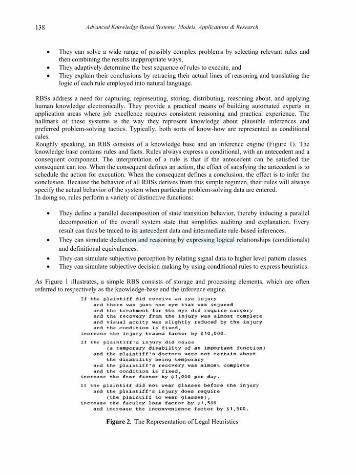
Figure 2. The Representation of Legal Heuristics


139

The basic cycle of an RBS consists of a select phase and an execute phase. During the execute phase, the system interprets the selected rule to draw inferences that alter the system’s dynamic memory. System storage includes components for long-term static data and short-term dynamic data. The long term store, which is the knowledge-base, contains rules and facts. Rules specify actions the system should initiate when certain triggering conditions occur. These conditions define important patterns of data that can arise in working memory. The system represents data in terms of relations, propositions, or equivalent logical expressions. Facts define static and true propositions.

Figure 1.The Basic Features of a RBS In contrast to conventional data-processing systems, most RBSs distribute their logic over numerous independent condition-action rules, monitor dynamic results for triggering patterns of data, determine their sequential behavior by selecting their next activity from a set of candidate triggered rules, and store their intermediate results exclusively in a global working memory. 3.2 Fuzzy Rule-Based Systems Fuzzy logic was initiated in 1965 by Lotfi A. Zadeh, professor in Computer Science at the University of California in Berkeley. Since then, Fuzzy logic has emerged as a powerful technique for the controlling industrial processes, household and entertainment electronics, diagnosis systems and other expert systems. Rapid growth of this technology has actually started from Japan and then spread to the USA and Europe. The motivation for fuzzy logic was expressed by Zadeh (1984) in the following way: "The ability of the human mind to reason in fuzzy terms is actually of a great advantage. Even though a tremendous amount of information is presented to the human senses in a given situation – an amount that would choke a typical computer – somehow the human mind has the ability to discard most of this information and to concentrate only on the information that is task relevant. This ability of the human mind to deal only with the information that is task relevant is connected with its possibility to process fuzzy information. By concentrating only on the task-relevant information, the amount of information the brain has to deal with is reduced to a manageable level".


140

140

Fuzzy logic is basically a multi-valued logic that allows intermediate values to be defined between conventional evaluations like yes/no, true/false, black/white, etc. Notions like rather warm or pretty cold can be formulated mathematically and algorithmically processed. In this way, an attempt is made to apply a more human-like way of thinking in the programming of computers ("soft" computing). Fuzzy logic systems address the imprecision of the input and output variables by defining fuzzy numbers and fuzzy sets that can be expressed in linguistic variables (e.g. small, medium, and large). Fuzzy rule-based approach to modeling is based on verbally formulated rules overlapped throughout the parameter space. They use numerical interpolation to handle complex non-linear relationships. Fuzzy rules are linguistic IF-THEN- constructions that have the general form "IF A THEN B" where A and B are (collections of) propositions containing linguistic variables. A is called the premise and B is the consequence of the rule. In effect, the use of linguistic variables and fuzzy IF-THEN- rules exploits the tolerance for imprecision and uncertainty. In this respect, fuzzy logic mimics the crucial ability of the human mind to summarize data and focus on decision-relevant information. A more explicit form, we can generate FRBs with one of the following three types of rules:

• Fuzzy rules with a class in the consequent. This kind of rules has the following structure:

kR : if 1x is klA and … and Nx is k

NA then Y is Cj Where 1x ... Nx are the outstanding selected features for the classification problem. k

lA ... kNA are

linguistic labels used to discretize the continuous domain of the variables, and Y is the class Cj to which the pattern belongs.

• Fuzzy rules with a class and certainty degree in the consequent.


NA then Y is Cj with kr Where, kr is the certainty degree of the classification in the class Cj for a pattern belonging to the

fuzzy subspace delimited by the antecedent. This degree can be determined by the ratio k

kj

SS

. Where,

considering the matching degree as the compatibility degree between the rule antecedent and the pattern feature values.

kjS is the sum of the matching degrees for the class Cj patterns belonging to the fuzzy region delimited

by the antecedent, and is the sum of the matching degrees for all the patterns belonging to this fuzzy subspace, regardless its associated class.

• Fuzzy rules with certainty degree for all classes in the consequent.


NA then ( kM

k rr ,...,1 )

Where, kr1 is the soundness degree for the rule k to predict the class Cj for a pattern belonging to the fuzzy region represented by the antecedent of the rule. This degree of certainty can be determined by the same ratio as the type b) rules. A Fuzzy Reasoning Method (FRM) is an inference procedure that derives conclusions from a set of fuzzy if-then rules and a pattern. The power of fuzzy reasoning is that we can achieve a result even when we do not have an exact match between a system observation and the antecedents of the rules.


141

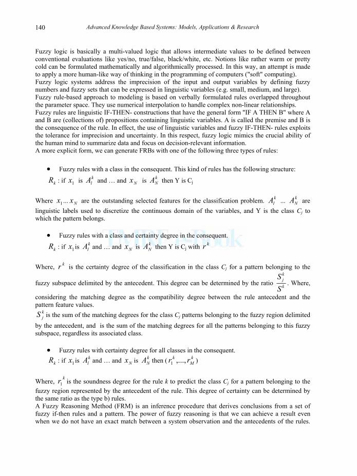
Here, we only explain a classical FRM (Maximum Matching) although there are various methods, which you can find in [Zadeh, 1992] and [Cordon et al., 1999]. Suppose that the RB is R={ 1R ,…, LR } and there are Lj rules in R that produce class Cj. Clearly, in an RB type c), Lj = L and j = 1,… M. For a pattern Et = ( te1 , …, t

Ne ), the classical fuzzy reasoning method considers the rule with the highest combination between the matching degree of the pattern with the if-part and the certainty degree for the classes. It classifies Et with the class that obtains the highest value. This procedure can be described in the following steps.

• Let Rk(Et) denote the strength of activation of the if-part of the rule k (matching degree).

Usually Rk(Et) is obtained by applying a t-norm to the degree of satisfaction of the clauses

( ix is kiA )

) )(e ( ,… )),(e ( T =)( tNA

t1A k

NkN

μμtk ER (7)

• Let h( )( tk ER , kjr )denote the degree of association of the pattern with class Cj according to

the rule k. This degree is obtained by applying a combination operator between )( tk ER and k

jr . For this operator, we can use the minimum and product ones or the product and the arithmetic means.

For each class Cj, the degree of association of the pattern with the class, Yj , is calculated by

)),((max kj

tkLkj rERhY

j∉= (8)

This degree of association is a soundness degree of the classification of the pattern Et in class Cj.

• The classification for the pattern Et is the class Ch such

jMjh YY ,...,1max == (9)

Figure2. Fuzzy Reasoning Method that uses only the winner rule


142

142

Graphically this method could be seen as shown in Figure 2. This reasoning method uses only one rule- the winner rule- in the inference process and wastes the information associated to all those rules whose association degree with the input pattern is lower than the association degree of the selected rule. If we only consider the rule with the highest association degree, we would not take into account the information of other rules with other fuzzy subsets which also have the value of the attribute in its support but to a lesser degree. 4. GENETIC FUZZY RULES BASED SYSTEM Fuzzy systems have been successfully applied to problems in classification, modeling, control [Driankov et al. 1993], and in a considerable number of applications. In most cases, the key for success was the ability of fuzzy systems to incorporate human expert knowledge. In the 1990s, despite the previous successful history, the lack of learning capabilities characterizing most of the works in the field generated a certain interest for the study of fuzzy systems with added learning capabilities. Two of the most successful approaches have been the hybridization attempts made in the framework of soft computing with different techniques, such as neural and evolutionary; provide fuzzy systems with learning capabilities, as shown in Figure 3. Neuro-fuzzy systems are one of the most successful and visible directions of that effort. A different approach to hybridization leads to Genetic Fuzzy Systems (GFSs) [Cordon et al. 2004] A GFS is basically a fuzzy system augmented by a learning process based on a GA. GA are search algorithms, based on natural genetics, that provide robust search capabilities in complex spaces, and thereby offer a valid approach to problems requiring efficient and effective search processes. Genetic learning processes cover different levels of complexity according to the structural changes produced by the algorithm, from the simplest case of parameter optimization to the highest level of complexity of learning the rule set of a rule based system. Parameter optimization has been the approach utilized to adapt a wide range of different fuzzy systems, as in genetic fuzzy clustering or genetic neuro-fuzzy systems. Analysis of the literature shows that the most prominent types of GFSs are Genetic Fuzzy Rule-Based Systems (GFRBSs), whose genetic process learns or tunes different components of a Fuzzy Rule-Based System (FRBS). Figure 4 shows this conception of a system where genetic design and fuzzy processing are the two fundamental constituents. Inside GFRBSs, it is possible to distinguish between either parameter optimization or rule generation processes, that is, adaptation and learning. A number of papers have been devoted to the automatic generation of the knowledge base of an FRBS using GA. The key point is to employ an evolutionary learning process to automate the design of the knowledge base, which can be considered as an optimization or search problem. From the viewpoint of optimization , the task of finding an appropriate Knowledge Base (KB) for a particular problem, is equivalent to parameterize the fuzzy KB (rules and membership functions), and to find those parameter values that are optimal with respect to the design criteria. The KB parameters constitute the optimization space, which is transformed into a suitable genetic representation in which the search process operates. The first step in designing a GFRBS is to decide which parts of the KB are subject to optimization by the GA. The KB of an FRBS does not constitute a homogeneous structure but is rather the union of qualitatively different components. As an example, the KB of a descriptive Mamdani-type FRBS (the one considered in Figure 5) is comprised of two components:A Data Base (DB), containing the definitions of the scaling functions of the variables and the membership functions of the fuzzy sets associated with the linguistic labels, and A Rule Base (RB), constituted by the collection of fuzzy rules.


143

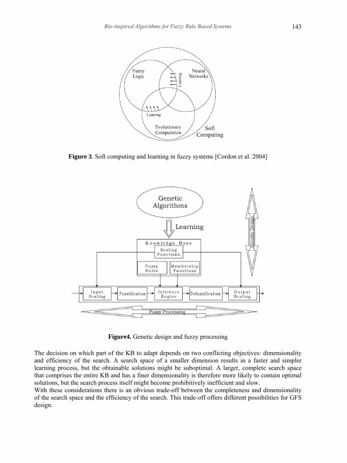
Figure 3. Soft computing and learning in fuzzy systems [Cordon et al. 2004]

Figure4. Genetic design and fuzzy processing The decision on which part of the KB to adapt depends on two conflicting objectives: dimensionality and efficiency of the search. A search space of a smaller dimension results in a faster and simpler learning process, but the obtainable solutions might be suboptimal. A larger, complete search space that comprises the entire KB and has a finer dimensionality is therefore more likely to contain optimal solutions, but the search process itself might become prohibitively inefficient and slow. With these considerations there is an obvious trade-off between the completeness and dimensionality of the search space and the efficiency of the search. This trade-off offers different possibilities for GFS design.


144

144

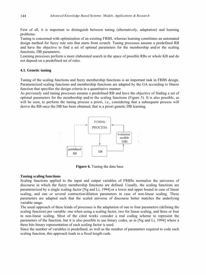
First of all, it is important to distinguish between tuning (alternatively, adaptation) and learning problems: Tuning is concerned with optimization of an existing FRBS, whereas learning constitutes an automated design method for fuzzy rule sets that starts from scratch. Tuning processes assume a predefined RB and have the objective to find a set of optimal parameters for the membership and/or the scaling functions, DB parameters. Learning processes perform a more elaborated search in the space of possible RBs or whole KB and do not depend on a predefined set of rules. 4.1. Genetic tuning Tuning of the scaling functions and fuzzy membership functions is an important task in FRBS design. Parameterized scaling functions and membership functions are adapted by the GA according to fitness function that specifies the design criteria in a quantitative manner. As previously said tuning processes assume a predefined RB and have the objective of finding a set of optimal parameters for the membership and/or the scaling functions (Figure 5). It is also possible, as will be seen, to perform the tuning process a priori, i.e., considering that a subsequent process will derive the RB once the DB has been obtained, that is a priori genetic DB learning.

Figure 6. Tuning the data base Tuning scaling functions Scaling functions applied to the input and output variables of FRBSs normalize the universes of discourse in which the fuzzy membership functions are defined. Usually, the scaling functions are parameterized by a single scaling factor [Ng and Li, 1994] or a lower and upper bound in case of linear scaling, and one or several contraction/dilation parameters in case of non-linear scaling. These parameters are adapted such that the scaled universe of discourse better matches the underlying variable range. The usual approach of these kinds of processes is the adaptation of one to four parameters (defining the scaling function) per variable: one when using a scaling factor, two for linear scaling, and three or four in non-linear scaling. Most of the cited works consider a real coding scheme to represent the parameters of the function, but it is also possible to use binary codes, as in [Ng and Li, 1994] where a three bits binary representation of each scaling factor is used. Since the number of variables is predefined, as well as the number of parameters required to code each scaling function, this approach leads to a fixed length code.


145

Tuning membership functions When tuning membership functions, an individual represents the entire DB as its chromosome encodes the parameterized membership functions associated to the linguistic terms in every fuzzy partition considered by the FRBS. The most common shapes for the membership functions (in GFRBSs) are triangular (either isosceles or asymmetric), trapezoidal or Gaussian functions. The number of parameters per membership function usually ranges from one to four, each parameter being either binary or real coded. The structure of the chromosome is different for FRBSs of the descriptive (using linguistic variables) or the approximate (using fuzzy variables) type. When tuning the membership functions in a linguistic model, the entire fuzzy partitions are encoded into the chromosome and it is globally adapted to maintain the global semantic in the RB. These approaches usually consider a predefined number of linguistic terms for each variable (no need to be the same for each of them), leading to a code of fixed length in what concerns membership functions. But even having a fixed length for the code, it is possible to evolve the number of linguistic terms associated to a variable by simply defining a maximum number (that defines the length of the code) and letting some of the membership functions to be located out of the range of the linguistic variable (reducing the actual number of linguistic terms). This is the conception that is used when designing a TSK system with linguistic input variables. A particular case, where the number of parameters to be coded is reduced, is that of descriptive fuzzy systems working with strong fuzzy partitions. In this case, the number of parameters to code is reduced to those defining the core regions of the fuzzy sets: the modal point for triangles, the extreme points of the core for trapezoidal shapes. On the other hand, tuning the membership functions of a model working with fuzzy variables (scatter partitions) is a particular instantiation of KB learning since the rules are completely defined by their own membership functions instead of referring to linguistic terms in the DB.

4.2. Genetic learning of rule bases

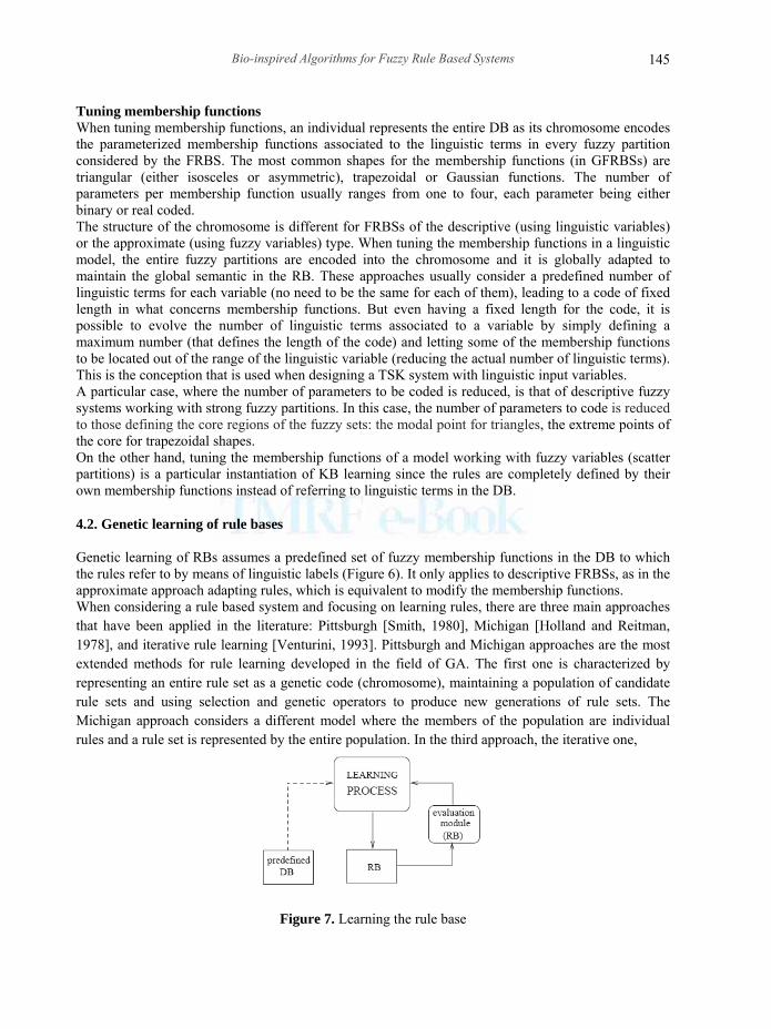
Genetic learning of RBs assumes a predefined set of fuzzy membership functions in the DB to which the rules refer to by means of linguistic labels (Figure 6). It only applies to descriptive FRBSs, as in the approximate approach adapting rules, which is equivalent to modify the membership functions. When considering a rule based system and focusing on learning rules, there are three main approaches that have been applied in the literature: Pittsburgh [Smith, 1980], Michigan [Holland and Reitman, 1978], and iterative rule learning [Venturini, 1993]. Pittsburgh and Michigan approaches are the most extended methods for rule learning developed in the field of GA. The first one is characterized by representing an entire rule set as a genetic code (chromosome), maintaining a population of candidate rule sets and using selection and genetic operators to produce new generations of rule sets. The Michigan approach considers a different model where the members of the population are individual rules and a rule set is represented by the entire population. In the third approach, the iterative one,

Figure 7. Learning the rule base


146

146

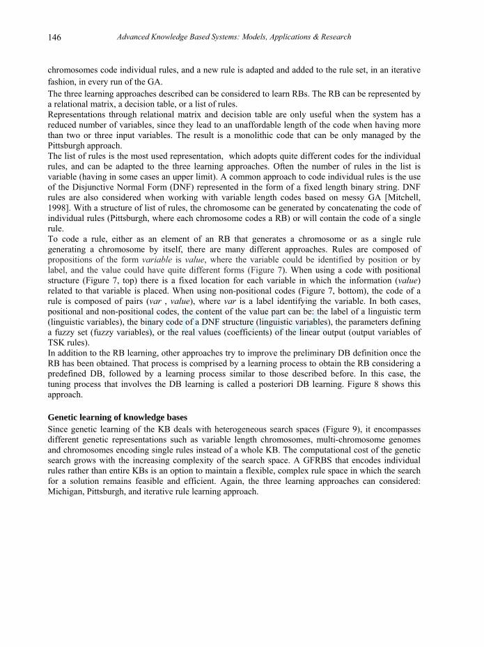
chromosomes code individual rules, and a new rule is adapted and added to the rule set, in an iterative fashion, in every run of the GA. The three learning approaches described can be considered to learn RBs. The RB can be represented by a relational matrix, a decision table, or a list of rules. Representations through relational matrix and decision table are only useful when the system has a reduced number of variables, since they lead to an unaffordable length of the code when having more than two or three input variables. The result is a monolithic code that can be only managed by the Pittsburgh approach. The list of rules is the most used representation, which adopts quite different codes for the individual rules, and can be adapted to the three learning approaches. Often the number of rules in the list is variable (having in some cases an upper limit). A common approach to code individual rules is the use of the Disjunctive Normal Form (DNF) represented in the form of a fixed length binary string. DNF rules are also considered when working with variable length codes based on messy GA [Mitchell, 1998]. With a structure of list of rules, the chromosome can be generated by concatenating the code of individual rules (Pittsburgh, where each chromosome codes a RB) or will contain the code of a single rule. To code a rule, either as an element of an RB that generates a chromosome or as a single rule generating a chromosome by itself, there are many different approaches. Rules are composed of propositions of the form variable is value, where the variable could be identified by position or by label, and the value could have quite different forms (Figure 7). When using a code with positional structure (Figure 7, top) there is a fixed location for each variable in which the information (value) related to that variable is placed. When using non-positional codes (Figure 7, bottom), the code of a rule is composed of pairs (var , value), where var is a label identifying the variable. In both cases, positional and non-positional codes, the content of the value part can be: the label of a linguistic term (linguistic variables), the binary code of a DNF structure (linguistic variables), the parameters defining a fuzzy set (fuzzy variables), or the real values (coefficients) of the linear output (output variables of TSK rules). In addition to the RB learning, other approaches try to improve the preliminary DB definition once the RB has been obtained. That process is comprised by a learning process to obtain the RB considering a predefined DB, followed by a learning process similar to those described before. In this case, the tuning process that involves the DB learning is called a posteriori DB learning. Figure 8 shows this approach. Genetic learning of knowledge bases Since genetic learning of the KB deals with heterogeneous search spaces (Figure 9), it encompasses different genetic representations such as variable length chromosomes, multi-chromosome genomes and chromosomes encoding single rules instead of a whole KB. The computational cost of the genetic search grows with the increasing complexity of the search space. A GFRBS that encodes individual rules rather than entire KBs is an option to maintain a flexible, complex rule space in which the search for a solution remains feasible and efficient. Again, the three learning approaches can considered: Michigan, Pittsburgh, and iterative rule learning approach.


147

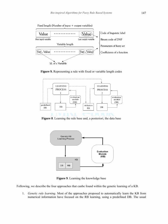
Figure 9. Representing a rule with fixed or variable length codes

Figure 8. Learning the rule base and, a posteriori, the data base

Figure 9. Learning the knowledge base

Following, we describe the four approaches that canbe found within the genetic learning of a KB.

1. Genetic rule learning. Most of the approaches proposed to automatically learn the KB from numerical information have focused on the RB learning, using a predefined DB. The usual


148

148

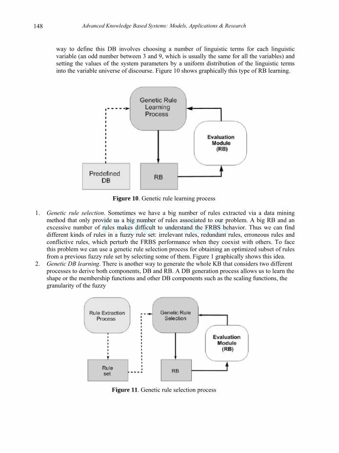
way to define this DB involves choosing a number of linguistic terms for each linguistic variable (an odd number between 3 and 9, which is usually the same for all the variables) and setting the values of the system parameters by a uniform distribution of the linguistic terms into the variable universe of discourse. Figure 10 shows graphically this type of RB learning.

Figure 10. Genetic rule learning process

1. Genetic rule selection. Sometimes we have a big number of rules extracted via a data mining

method that only provide us a big number of rules associated to our problem. A big RB and an excessive number of rules makes difficult to understand the FRBS behavior. Thus we can find different kinds of rules in a fuzzy rule set: irrelevant rules, redundant rules, erroneous rules and conflictive rules, which perturb the FRBS performance when they coexist with others. To face this problem we can use a genetic rule selection process for obtaining an optimized subset of rules from a previous fuzzy rule set by selecting some of them. Figure 1 graphically shows this idea.

2. Genetic DB learning. There is another way to generate the whole KB that considers two different processes to derive both components, DB and RB. A DB generation process allows us to learn the shape or the membership functions and other DB components such as the scaling functions, the granularity of the fuzzy

Figure 11. Genetic rule selection process


149

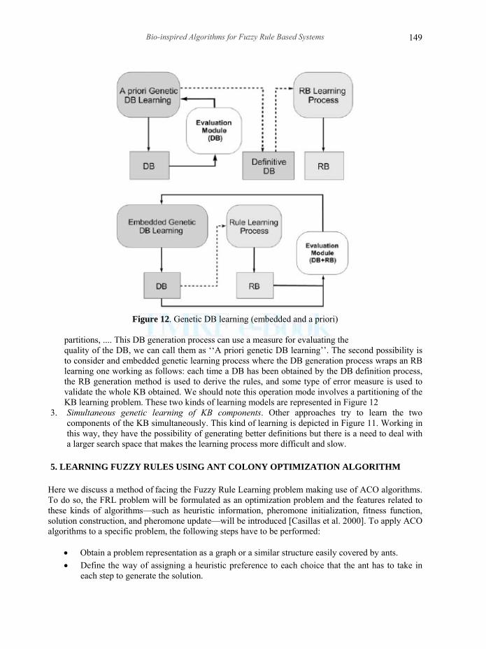
Figure 12. Genetic DB learning (embedded and a priori)

partitions, .... This DB generation process can use a measure for evaluating the quality of the DB, we can call them as ‘‘A priori genetic DB learning’’. The second possibility is to consider and embedded genetic learning process where the DB generation process wraps an RB learning one working as follows: each time a DB has been obtained by the DB definition process, the RB generation method is used to derive the rules, and some type of error measure is used to validate the whole KB obtained. We should note this operation mode involves a partitioning of the KB learning problem. These two kinds of learning models are represented in Figure 12

3. Simultaneous genetic learning of KB components. Other approaches try to learn the two components of the KB simultaneously. This kind of learning is depicted in Figure 11. Working in this way, they have the possibility of generating better definitions but there is a need to deal with a larger search space that makes the learning process more difficult and slow.

5. LEARNING FUZZY RULES USING ANT COLONY OPTIMIZATION ALGORITHM Here we discuss a method of facing the Fuzzy Rule Learning problem making use of ACO algorithms. To do so, the FRL problem will be formulated as an optimization problem and the features related to these kinds of algorithms—such as heuristic information, pheromone initialization, fitness function, solution construction, and pheromone update—will be introduced [Casillas et al. 2000]. To apply ACO algorithms to a specific problem, the following steps have to be performed:

• Obtain a problem representation as a graph or a similar structure easily covered by ants. • Define the way of assigning a heuristic preference to each choice that the ant has to take in

each step to generate the solution.


150

150

• Establish an appropriate way of initializing the pheromone. • Define a fitness function to be optimized. • Select an ACO algorithm and apply it to the problem.

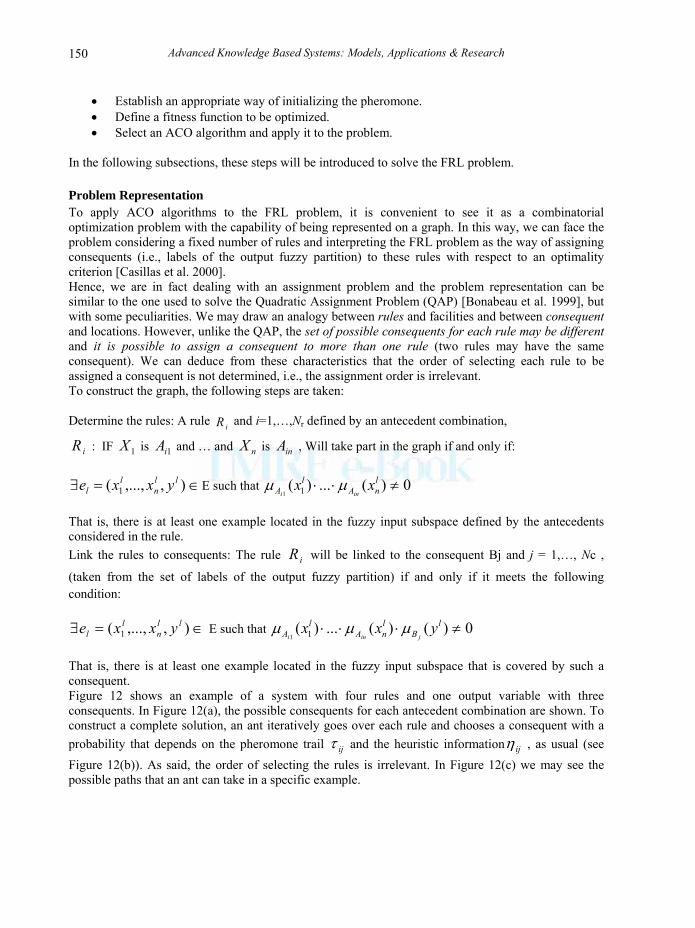
In the following subsections, these steps will be introduced to solve the FRL problem. Problem Representation To apply ACO algorithms to the FRL problem, it is convenient to see it as a combinatorial optimization problem with the capability of being represented on a graph. In this way, we can face the problem considering a fixed number of rules and interpreting the FRL problem as the way of assigning consequents (i.e., labels of the output fuzzy partition) to these rules with respect to an optimality criterion [Casillas et al. 2000]. Hence, we are in fact dealing with an assignment problem and the problem representation can be similar to the one used to solve the Quadratic Assignment Problem (QAP) [Bonabeau et al. 1999], but with some peculiarities. We may draw an analogy between rules and facilities and between consequent and locations. However, unlike the QAP, the set of possible consequents for each rule may be different and it is possible to assign a consequent to more than one rule (two rules may have the same consequent). We can deduce from these characteristics that the order of selecting each rule to be assigned a consequent is not determined, i.e., the assignment order is irrelevant. To construct the graph, the following steps are taken: Determine the rules: A rule iR and i=1,…,Nr defined by an antecedent combination,

iR : IF 1X is 1iA and … and nX is inA , Will take part in the graph if and only if:

),,...,( 1ll

nl

l yxxe =∃ ∈E such that 0)(...)( 11≠⋅⋅ l

nAl

A xxini

μμ That is, there is at least one example located in the fuzzy input subspace defined by the antecedents considered in the rule. Link the rules to consequents: The rule iR will be linked to the consequent Bj and j = 1,…, Nc ,

(taken from the set of labels of the output fuzzy partition) if and only if it meets the following condition:

),,...,( 1ll

nl

l yxxe =∃ ∈ E such that 0)()(...)( 11≠⋅⋅⋅ l

BlnA

lA yxx

jiniμμμ

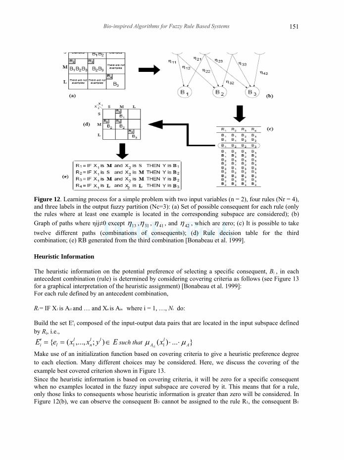
That is, there is at least one example located in the fuzzy input subspace that is covered by such a consequent. Figure 12 shows an example of a system with four rules and one output variable with three consequents. In Figure 12(a), the possible consequents for each antecedent combination are shown. To construct a complete solution, an ant iteratively goes over each rule and chooses a consequent with a probability that depends on the pheromone trail ijτ and the heuristic information ijη , as usual (see Figure 12(b)). As said, the order of selecting the rules is irrelevant. In Figure 12(c) we may see the possible paths that an ant can take in a specific example.


151

Figure 12. Learning process for a simple problem with two input variables (n = 2), four rules (Nr = 4), and three labels in the output fuzzy partition (Nc=3): (a) Set of possible consequent for each rule (only the rules where at least one example is located in the corresponding subspace are considered); (b) Graph of paths where ηij≠0 except 13η , 31η , 41η , and 42η , which are zero; (c) It is possible to take twelve different paths (combinations of consequents); (d) Rule decision table for the third combination; (e) RB generated from the third combination [Bonabeau et al. 1999]. Heuristic Information

The heuristic information on the potential preference of selecting a specific consequent, Bj , in each antecedent combination (rule) is determined by considering covering criteria as follows (see Figure 13 for a graphical interpretation of the heuristic assignment) [Bonabeau et al. 1999]: For each rule defined by an antecedent combination, Ri = IF X1 is Ai1 and … and Xn is Ain where i = 1, …, Nr do:

Build the set E'i composed of the input-output data pairs that are located in the input subspace defined by Ri, i.e.,

EyxxeE lln

lli ∈==′ );,...,({ 1 such that }...)( 11 A

lA x

iμμ ⋅⋅

Make use of an initialization function based on covering criteria to give a heuristic preference degree to each election. Many different choices may be considered. Here, we discuss the covering of the example best covered criterion shown in Figure 13. Since the heuristic information is based on covering criteria, it will be zero for a specific consequent when no examples located in the fuzzy input subspace are covered by it. This means that for a rule, only those links to consequents whose heuristic information is greater than zero will be considered. In Figure 12(b), we can observe the consequent B3 cannot be assigned to the rule R1, the consequent B1


152

152

cannot be assigned to the rule R3, and the consequents B1 and B2 cannot be assigned to the rule R4 because their heuristic information (covering degrees) are zero. Pheromone Initialization

The initial pheromone value of each assignment is obtained as follows:

τ0 = r

N

i ijNj

N

r c∑ = =1 1max η.In this way, the initial pheromone will be the mean value of the path

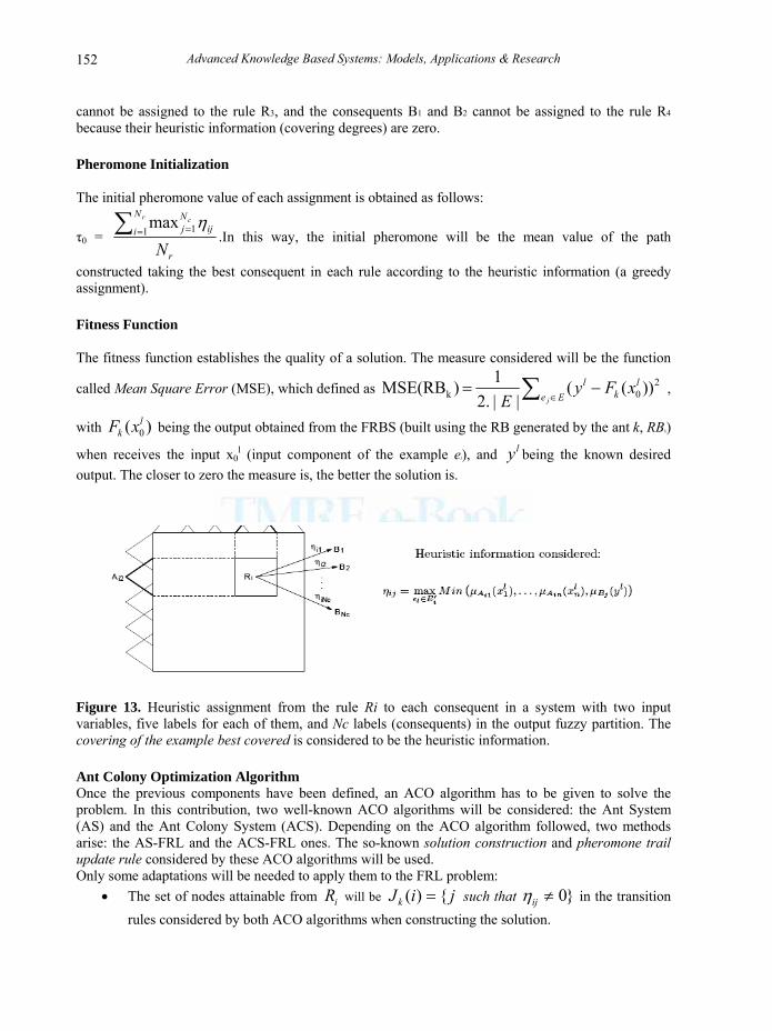
constructed taking the best consequent in each rule according to the heuristic information (a greedy assignment). Fitness Function

The fitness function establishes the quality of a solution. The measure considered will be the function

called Mean Square Error (MSE), which defined as ∑ ∈−=

Eel

kl

jxFy

E2

0k ))((||.2

1 )MSE(RB ,

with )( 0l

k xF being the output obtained from the FRBS (built using the RB generated by the ant k, RBk)

when receives the input x0l (input component of the example el), and ly being the known desired

output. The closer to zero the measure is, the better the solution is.

Figure 13. Heuristic assignment from the rule Ri to each consequent in a system with two input variables, five labels for each of them, and Nc labels (consequents) in the output fuzzy partition. The covering of the example best covered is considered to be the heuristic information. Ant Colony Optimization Algorithm Once the previous components have been defined, an ACO algorithm has to be given to solve the problem. In this contribution, two well-known ACO algorithms will be considered: the Ant System (AS) and the Ant Colony System (ACS). Depending on the ACO algorithm followed, two methods arise: the AS-FRL and the ACS-FRL ones. The so-known solution construction and pheromone trail update rule considered by these ACO algorithms will be used. Only some adaptations will be needed to apply them to the FRL problem:

• The set of nodes attainable from iR will be jiJk {)( = such that }0≠ijη in the transition rules considered by both ACO algorithms when constructing the solution.


153

• The amount of pheromone ant k puts on the couplings belonging to the solution constructed by it will be )(/1 kRBMSE , with kRB being the RB generated by ant k.

• In the local pheromone trail update rule of the ACS algorithm, the most usual way of calculating 0, τττ =ΔΔ ijij , will be used, thus considering the simple-ACS algorithm.

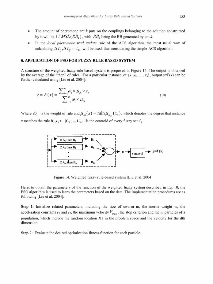
6. APPLICATION OF PSO FOR FUZZY RULE BASED SYSTEM A structure of the weighted fuzzy rule-based system is proposed in Figure 14. The output is obtained by the average of the “then” of rules. For a particular instance x= {x1,x2, …, xn}, output y=F(x) can be further calculated using [Liu et al. 2004]:

∑∑

=

=

×

××== m

i iki

m

i iiki cxFy

1

1)(μω

μω

(10)

Where iω is the weight of rule and )(min)(1 nRRi xx

nμμ = , which denotes the degree that instance

x matches the rule },...,{, 1 Mii CCcR ∈ is the centroid of every fuzzy set Ci.

Figure 14. Weighted fuzzy rule-based system [Liu et al. 2004]

Here, to obtain the parameters of the function of the weighted fuzzy system described in Eq. 10, the PSO algorithm is used to learn the parameters based on the data. The implementation procedures are as following [Liu et al. 2004]:

Step 1: Initialize related parameters, including the size of swarm m, the inertia weight w, the acceleration constants c1 and c2, the maximum velocity maxV , the stop criterion and the m particles of a population, which include the random location X1 in the problem space and the velocity for the dth dimension.

Step 2: Evaluate the desired optimization fitness function for each particle.


154

154

Step 3: Compare the evaluated fitness value of each particle with its bestP . If current value is better

than bestP then set the current location as the bestP location. Furthermore, if current value is better

than bestg , then reset bestg to the current index in particle array.

Step 4: Change the velocity and location of the particle according to the Eqs. 11a and 11b, respectively.

)()( 22111 n

idnid

nnid

nid

nnid

nid xprcxprcwvV −+−+=+

(11a)

11 ++ += nid

nid

nid vxX (11b)

Step 5: Loop to step 2 until a stopping criterion is met. The criterion usually is a sufficiently good fitness value or a predefined maximum number of generations Gmax. The fitness function mentioned in step 2 and step 3 for the weighted fuzzy rule-based system identification is given as:

∑ =−=

n

kkykytJ

12)](ˆ)([)( (12)

Where J = cost function to be minimized, y = system output, y = model output, and k= 1, 2, …, n. n denotes the number of sample data.

Parameters Learning by PSO Algorithm

Before PSO parameter learning stage, the initial feature of the population for PSO should be defined. This can be done for example via cluster centers driven by popular FCM. These initial values will sequentially be assigned to the premise ( ia ) and the consequent part ( iy ) of the fuzzy set. Normally,

the parameter set ( ib ) is determined by random operation. Note that every particle’s position is made

up of parameter set ( ija , ijb and iy ) and its velocity is initiated as same dimension as position by random process. At the learning iteration, each particle’s position (px) and velocity (pv) values are adjusted by two best information. The first best one, called Pbest_px, is every particle’s best solution (highest fitness) which has been achieved so far. The other best value, called Gbest_px, is obtained by choosing the overall best value from all particles. It is known that this useful information is good for all swarms to share their best knowledge. At the learning step, the velocity of every particle is modified according to the relative Pbest_px and Gbest_px. The new velocity is updated by the following equation[Feng H.M.; 2006]:

)1(2))()1(_)(1(1)()1( ,,,,,, ++−+++=+ ttpxtpxPbestttpvtpv dpdpdpdpdpdp αα

ndtpxtpxGbest dpdp ≤≤−+ 1)),()1(_( ,, (13)


155

Where dppv , and dppx , are respectively the pth velocity and position. Here, p is the number of

particles; d the number of dimension. t employs current state, t + 1 denotes the next time step, dp,1α

(t + 1) and )1(2 , +tdpα are random number between 0 and 1. Since the velocity of the particle is determined, the next particle’s location will be modified by:

)1()()1( ,,, ++=+ tpvtpxtpx dpdpdp (14) Based on (13) and (14) the direction of every particle will regulate its original flying path with the factor of Gbest_px and Pbest_px.

7. IMMINENT TRENDS

The hybridization of fuzzy logic and EC in Genetic Fuzzy Systems became an important research area during the last decade. To date, several hundred papers, special issues of different journals and books have been devoted [cordon et al. 2001], [Cordon, et al. 2004]. Nowadays, as the field of GFSs matures and grows in visibility, there is an increasing concern on the integration of these two topics from a novel and more sophisticated perspective. In what follows, we enumerate some open questions and scientific problems that suggest future research: Hybrid intelligent systems balance between interpretability and accuracy, and sophisticated evolutionary algorithms. As David Goldberg stated [Goldberg, 2004], the integration of single methods into hybrid intelligent systems goes beyond simple combinations [Cordon et al., 2004]. Other evolutionary learning models, as seen, the three classical genetic learning approaches are Michigan, Pittsburgh and Iterative Rule Learning. Improving mechanisms for these approaches or the development of other new ones may be necessary [Cordon et al., 2004].

8. CONCLUSION

In this chapter we focused on three bio-inspired algorithms and their combination with fuzzy rule based systems. Rule Based systems are widely being used in decision making, control systems and forecasting. In the real world, much of the knowledge is imprecise and ambiguous but fuzzy logic provides our systems a better presentation of the knowledge, which is in terms of the natural language. Fuzzy rule based systems constitute an extension of classical Rule-Based Systems, because they deal with fuzzy rules instead of classical logic rules. As we said, the generation of the Knowledge Base (KB) of a Fuzzy Rule Based System (FRBS) presents several difficulties because the KB depends on the concrete application, and this makes the accuracy of the FRBS directly depend on its composition. Many approaches have been proposed to automatically learn the KB from numerical information. Most of them have focused on the Rule Base (RB) learning, using a predefined data base (DB). This operation mode makes the DB have a significant influence on the FRBS performance. In fact, some studies have shown that the system performance is much more sensitive to the choice of the semantics in the DB than to the composition of the RB. The usual solution for improving the FRBS performance by dealing with the DB components involves a tuning process of the preliminary DB definition once the RB has been derived. This process only adjusts the membership function definitions and does not modify the number of linguistic terms in each fuzzy partition since the RB remains unchanged.


156

156

Using bio-inspired optimization algorithms have been shown effective in improving the tuning the parameters and learning the Fuzzy Rule Base. Thus, we began by introducing the EC and Swarm Intelligence as a subfield of Computational Intelligence that involves Combinatorial Optimization problems and then three following bio-inspired algorithms, i.e. GA, Ant Colony, and PSO were explained. We also represented the usage of these algorithms in improving the Knowledge Based systems with focus on Rule Base Learning. In this context we emphasized the need to build hybrid intelligent systems that go beyond simple combinations. Development of GFSs that offer acceptable trade-off between interpretability and accuracy is also a major requirement for efficient and transparent knowledge extraction. The hybridization between fuzzy systems and GAs in GFSs became an important research area during the last decade. GAs allow us to represent different kinds of structures, such as weights, features together with rule parameters, etc., allowing us to code multiple models of knowledge representation. This provides a wide variety of approaches where it is necessary to design specific genetic components for evolving a specific representation. Nowadays, it is a mature research area, where researchers need to reflect in order to advance towards strengths and distinctive features of the GFSs, providing useful advances in the fuzzy systems theory. In this chapter also, an interesting application, the FRL problem (which involves automatically learning from numerical data the RB composing an FRBS), has been proposed to be solved by the ACO meta-heuristic. In this way, an ACO-based learning method has been presented. Comparing with other ad hoc learning algorithms, the models obtained by the ACO methods are clearly better. Moreover, opposite to other kinds of optimization techniques such as SA and GA, the ACO approach performs a quick convergence and sometimes obtains better results. The former is due to the use of heuristic information to guide the global search. Then, as it was shown, based on the fuzzy rule-based system, we can assign a weight to every fuzzy rule to construct a weighted fuzzy rule-based system. The PSO algorithm can be used to estimate the parameters of the weighted fuzzy rule-based system, which include the position and the shape of membership function, fuzzy rules and its weights. The PSO algorithm is effective in the procedure of obtaining the parameters of the weighted fuzzy system. As we said, fuzzy system with weights could get better results compared with the one without weights.

REFERENCES

Back T., Schwefel H.P. [1986] An overview of Evolutionary Algorithm for Parameter Optimization, Springer Verlag, New York-1986

Bárdossy A., Duckstein L.; [1995]; Fuzzy rule-based modeling with applications to geophysical; CRC Press. Bonabeau E., Dorigo M., and Theraulaz G.; [1999]; swarm intelligence from natural to artificial systems; Oxford University Press.

Bonabeau E., Dorigo M., Theraulaz G.; [2000]; Nature; Vol. 406; 6791, 39-42. Driankov D., Hellendoorn H., Reinfrank M.;[ 1993]; An Introduction to Fuzzy Control; Springer, Berlin. Casillas J., Cordon O., Herrera F.; [1999]; Learning Fuzzy Rules Using Ant Colony Optimization Algorithms; Ant Colonies to Arti Ants: A Series of International Workshops on Ant Algorithms;


157

Chi Z., Yan H., and Pham T.; [1996]; Fuzzy algorithms: With applications to image processing and pattern recognition; Advances in Fuzzy Systems-Application and Theory; Vol. 10; World Scientific. Cordon, O., Del Jesus, M.J. and Herrera, F.; [1999]; A proposal on reasoning methods in fuzzy rule-based classification systems; International Journal of Approximate reasoning. 20. 21-45. Cordon O, Gomide F., Herrera F., Hoffmann L., Magdalena L.;[2004];Ten years of genetic fuzzy systems: current framework and new trends; Fuzzy Sets and Systems; 141; 5–31; Cordón O., Herrera F., and Villar P.; [1998]; Generating the Knowledge Base of a Fuzzy Rule-Based System by the Genetic Learning of the Data Base; International journal of intelligent systems; 13, 1025-1053. Cordon O., Herrera F., Hoffmann F., and Magdalena L.; [2001]; Genetic fuzzy systems: evolutionary tuning and learning of fuzzy knowledge bases; Vol. 16; World Scientific (Advances in Fuzzy Systems-Application and Theory). Dorigo M.; [1992]; Optimization, Learning and Natural Algorithms, PhD thesis, Politecnico di Milano, Italie. Dorigo M. and Gambardella L. M.; [1997]; Ant colony system: a cooperative learning approach to the traveling salesman problem, IEEE Transaction on Evolutionary Computation; 1;53--66. Eiben A. E. and Smith J. E.; [2003]; introduction to evolutionary computing; Springer,Natural Computing Series. Engelbrecht P.; [2007]; Computational Intelligence: An Introduction, 2nd Edition; Wiley. Feng H.F.; [2006]; Hybrid Stages Particle Swarm Optimization Learning Fuzzy Modeling Systems Design; Journal of Science and Engineering, Vol. 9, No 2, pp. 167-176 Fisher, R. A.; [1911]; Mendelism and biometr; Unpublished Gambardella L.M. and M. Dorigo M.; [1995]; Ant-Q: a reinforcement learning approach to the travelling salesman problem, Proceedings of the Twelfth International Conference on Machine Learning, ML-95, Palo Alto, CA, Morgan Kaufmann, Palo Alto: California, USA,. Goldberg D. E.; [1989]; Genetic algorithms in search, optimization, and machine learning; Addison-Wesley: New York. Goldberg D. E.; [2000]; A meditation on the computational intelligence and its future, Technical Report ; Illinois Genetic Algorithms Laboratory, University of Illinois at Urbana-Champaign, Foreword of the Proc. Int. Symp. on Computational Intelligence. Holland J.H., Reitman J.S.; [1978], Cognitive systems based on adaptive algorithms, D.A. Waterman, F. Hayes-Roth (Eds.), Pattern-Directed Inference Systems, Academic Press, New York, 313–329.


158

158

Kennedy J., Eberhart R.C.; [1995]; Particle Swarm Optimization, Proceedings of IEEE international conference on neural networks, IV, pages 1942--1948, Piscataway, NJ, 1995. IEEE Service Center

Kennedy J. and Eberhart R. C.; [2001]; Swarm Intelligence; Morgan Kaufmann Publishers: San Francisco. Klir, G. and Yuan, B.; [1995]; Sets and Fuzzy Logic, Theory and Applications; Prentice Hall. Leondes T; [1999]; Fuzzy Theory Systems: Techniques and Applications; Academic Press, Inc. Lin S. and Kernighan B.W.; [1973]; An effective heuristic algorithm for the traveling salesman Problem; Operations Research, 21, 498–516. L.M Gambardella and M. Dorigo M.; [1996]; Solving Symmetric and Asymmetric TSPs by Ant Colonies; Proceedings of the IEEE Conference on Evolutionary Computation, ICEC96, Nagoya, Japan, 622-627. Mamdani E.H. ; [1982]; A fuzzy rule-based method of controlling dynamic processes, IEEE Xplore Volume: 20, pp. 1098-1103 Maniezzo V. ,Gambardella L. M., Luigi F. D.; [2004]; Optimization Techniques in Engineering; Chapter 5; Springer-Verlag. Mitchell M.; [1998]; An introduction to genetic algorithm; The MIT Press. Mitchell T.; [1997]; Machine Learning, International Edition: USA, McGrawHill. Ng K.C., Li Y.; [1994]; Design of sophisticated fuzzy logic controllers using genetic algorithms, Proc. 3rd IEEE Int.Conf. on Fuzzy Systems (FUZZ-IEEE’94), 3, Orlando, FL, USA, 1708–1712. Pedrycz W.; [1996]; Knowledge-based clustering: from data to information granules; Wiley «a». Pedrycz W.; [1996]; Fuzzy Modeling: Paradigms and Practices; Kluwer Academic Publishers «b». Smith S.F.; [1980]; A learning system based on genetic adaptive algorithms; Doctoral Dissertation, Department of Computer Science, University of Pittsburgh. Venturini G.; [1993]; SIA: a supervised inductive algorithm with genetic search for learning attribute based concepts, In Proc. European Conf. on Machine Learning, Vienna, 280–296. Yager R., Zadeh L. A.; [1992]; An Introduction to Fuzzy Logic Applications in Intelligent Systems; Kluwer Academic Publishers. Yijian Liu, Xuemei Zhu, Jianming Zhang, Shuqing Wang; [2004]; Application of Particle Swarm Optimization Algorithm for Weighted Fuzzy Rule-Based System;30th Annual Conference of the IEEE Industrial Electronics Society, Ousan, Korea. Yoshinari Y., Pedrycz W., and Hirota K.; [1993]; Construction of fuzzy models through clustering techniques; Fuzzy Sets and Systems; Vol. 54; Issue 2;157 - 165; Elsevier North-Holland, Inc.


159

Zadeh, L.A.; [1992]; The calculus of fuzzy if-then rules; AI Expert. Vol.7; 3, 23-27.

Zimmermann H.J. ; [1996]; Practical applications of fuzzy technologies; Springer.

bio-inspired algorithms for fuzzy rule-based systems · bio-inspired algorithms for fuzzy...

Documents