bifurcation analysis of nonlinear ground handling of aircraftrankin/jrankin_thesis.pdf ·...
TRANSCRIPT

Bifurcation Analysis of Nonlinear GroundHandling of Aircraft
James Rankin
Department of Engineering Mathematics
University of Bristol
A dissertation submitted to the University of Bristol in
accordance with the requirements of the degree of
Doctor of Philosophy in the Faculty of Engineering.
March 2010


Abstract
Nonlinearities inherent in the landing gear geometry, the complex interactions at the tyre-ground interface and the aerodynamics play an important role in the behaviour of aircraft onthe ground. The use of computer models that incorporate nonlinear effects is becoming morewidespread in industry. Numerical continuation and bifurcation analysis have successfullybeen applied in the study of road vehicle dynamics and flight dynamics. However, the study ofaircraft ground handling has not yet been approached in this way. Here, we work with computerand mathematical models that capture the important nonlinear effects in the relevant compo-nents to show that bifurcation and continuation methods provide an efficient and effective wayof investigating the highly nonlinear dynamics of an aircraft moving on the ground.
In order to investigate turning manoeuvres we utilise an established, industry-tested, multi-body systems model representing an Airbus A320 passenger aircraft. The model is linkeddirectly to the numerical continuation package AUTO without the need to derive the equationsof motion explicitly. Steady-state solutions of the system are fixed-radius turning circles. Wepresent a bifurcation study showing how these solutions change with respect to variation of twocontrol inputs: the steering angle and the thrust level. Identified are regions of stable turningand regions of laterally unstable behaviour; the transition between these types of behaviour isassociated with a Hopf bifurcation. A detailed study of the undesirable behaviour associatedwith a loss of lateral stability focuses on the saturation of tyre forces at different wheel sets. Thepresented bifurcation diagrams identify parameter regions for which undesirable behaviour isavoidable and, thus, they form a foundation for defining the safe operating limits during turningmanoeuvres.
Next we present the derivation and validation of a fully mathematical model that facili-tates more elaborate bifurcation studies in terms of additional operational parameters. Two-parameter bifurcation diagrams are represented in compact form as surfaces of solutions thatprovide complete descriptions of the overall dynamics. Under the variation of additional pa-rameters, qualitative changes to the solution structure are identified and the physical relevanceof these changes is explained. Our results give a full description of the possible turning dynam-ics of the aircraft in dependence on four parameters of operational relevance. With a combina-tion of numerical continuation and simulation we gain further insight into the mechanism bywhich lateral stability of the aircraft is lost. The system is shown to have a separation of timescales and to exhibit so-called canard-type oscillations; these phenomena are directly relatedto physical effects in the system.
To complement the bifurcation analysis of steady-state solutions, a transient analysis is pre-sented that takes into account the taxiway geometry and fully captures the aircraft’s behaviourduring the initialisation and execution of a turn. We introduce a general approach to assess anaircraft’s performance during taxiway manoeuvres across the range of its operation. The limitsof operating regions are determined from published data on the usage of in-service aircraft. Themaximal lateral loads experienced at individual landing gears are found, and this informationallows us to assess the suitability of existing regulations for the certification of aircraft. A com-parison between the steady-state and transient analysis shows that regions of safe operation asdefined in the bifurcation analysis are physically relevant and of practical importance.


Acknowledgements
The project was funded by an Engineering and Physical Sciences Research Council (EPSRC)Case award grant in collaboration with Airbus in the United Kingdom.
I would like to thank my supervisors Prof. Bernd Krauskopf, Dr. Mark Lowenberg andSanjiv Sharma for their continued support and encouragement. Without their guidance andexpertise this Ph.D. would not have been possible. I am truly grateful to Etienne Coetzee wholed the way and acted as a patient and insightful adviser throughout.
Thanks also to Mathieu Desroches, Clare Lee and Dave Rodrigues who taught me how todo everything in the beginning, and Phani Thota has always found the time to offer his help.During my time with the Engineering Mathematics Department I have made too many friendsto mention, safe to say, if we shared a few ales in the Hope and Anchor, I couldn’t have done itwithout you.
I am indebted to Paul Street and everyone that made my time in Bristol so unique. The lastfew summers will never escape my fondest memories. A special thank you to ‘Team Buzz’ whokept me on the straight and narrow in that all-important final summer and taught me humility,patience, tolerance, commitment and poypes as we wended our way through Italy.
My family have been right behind me every step of the way: a massive thank you.


“No good fish goes anywhere without a porpoise.”Lewis Carroll


Author’s Declaration
I declare that the work in this dissertation was carried out in accordance with the regulationsof the University of Bristol. The work is original except where indicated by special referencein the text and no part of the dissertation has been submitted for any other degree.
Any views expressed in the dissertation are those of the author and in no way representthose of the University of Bristol.
The dissertation has not been presented to any other University for examination either inthe United Kingdom or overseas.
Signed:
Dated:


Contents
1 Introduction 11.1 Research motivation and objectives . . . . . . . . . . . . . . . . . . . . . . . . 11.2 Review of existing work . . . . . . . . . . . . . . . . . . . . . . . . . . . . . 21.3 Thesis overview . . . . . . . . . . . . . . . . . . . . . . . . . . . . . . . . . . 3
2 Bifurcation analysis of turning solutions 52.1 Introduction . . . . . . . . . . . . . . . . . . . . . . . . . . . . . . . . . . . . 52.2 SIMMECHANICS model . . . . . . . . . . . . . . . . . . . . . . . . . . . . . 7
2.2.1 Tyre modelling . . . . . . . . . . . . . . . . . . . . . . . . . . . . . . 82.2.2 Modelling the oleos . . . . . . . . . . . . . . . . . . . . . . . . . . . 112.2.3 Modelling the aerodynamics . . . . . . . . . . . . . . . . . . . . . . . 12
2.3 Bifurcation analysis of aircraft turning . . . . . . . . . . . . . . . . . . . . . . 132.3.1 Low-thrust case . . . . . . . . . . . . . . . . . . . . . . . . . . . . . . 142.3.2 High-thrust case . . . . . . . . . . . . . . . . . . . . . . . . . . . . . 162.3.3 Two-parameter bifurcation diagrams . . . . . . . . . . . . . . . . . . . 18
2.4 Different types of periodic solution . . . . . . . . . . . . . . . . . . . . . . . . 192.4.1 Diagrammatic representation . . . . . . . . . . . . . . . . . . . . . . . 232.4.2 Detailed discussion of cases A–D . . . . . . . . . . . . . . . . . . . . 23
2.5 Discussion . . . . . . . . . . . . . . . . . . . . . . . . . . . . . . . . . . . . . 30
3 Operational parameter study 333.1 Introduction . . . . . . . . . . . . . . . . . . . . . . . . . . . . . . . . . . . . 333.2 Mathematical model . . . . . . . . . . . . . . . . . . . . . . . . . . . . . . . 34
3.2.1 Tyre modelling . . . . . . . . . . . . . . . . . . . . . . . . . . . . . . 383.2.2 Modelling the aerodynamics . . . . . . . . . . . . . . . . . . . . . . . 41
3.3 Validation of mathematical model . . . . . . . . . . . . . . . . . . . . . . . . 423.4 Two-parameter bifurcation study and sensitivity analysis . . . . . . . . . . . . 44
3.4.1 Heavy aircraft case . . . . . . . . . . . . . . . . . . . . . . . . . . . . 453.4.2 Light aircraft case . . . . . . . . . . . . . . . . . . . . . . . . . . . . 483.4.3 Qualitative changes of the surfaces of solutions with thrust . . . . . . . 50
3.5 The effect of reducing tyre friction coefficient . . . . . . . . . . . . . . . . . . 523.6 Periodic orbits as canard cycles . . . . . . . . . . . . . . . . . . . . . . . . . . 533.7 Discussion . . . . . . . . . . . . . . . . . . . . . . . . . . . . . . . . . . . . . 56
4 Lateral loads during typical taxiway turns 594.1 Introduction . . . . . . . . . . . . . . . . . . . . . . . . . . . . . . . . . . . . 59
4.1.1 Specific loading cases . . . . . . . . . . . . . . . . . . . . . . . . . . 62
i

ii CONTENTS
4.2 Generic parameterized turn . . . . . . . . . . . . . . . . . . . . . . . . . . . . 634.2.1 Trajectory geometry . . . . . . . . . . . . . . . . . . . . . . . . . . . 64
4.3 Operating region for typical taxiway turns . . . . . . . . . . . . . . . . . . . . 654.3.1 Relating parameterized turn trajectories to specific manoeuvres . . . . 664.3.2 Maximal lateral loading conditions and operating regions . . . . . . . . 68
4.4 Maximal lateral gear loads in operating regions . . . . . . . . . . . . . . . . . 704.5 Operating region for efficient turns . . . . . . . . . . . . . . . . . . . . . . . . 724.6 Comparison of transient analysis and continuation analysis . . . . . . . . . . . 744.7 Discussion . . . . . . . . . . . . . . . . . . . . . . . . . . . . . . . . . . . . . 76
5 Conclusion and outlook 795.1 Summary . . . . . . . . . . . . . . . . . . . . . . . . . . . . . . . . . . . . . 795.2 Future work . . . . . . . . . . . . . . . . . . . . . . . . . . . . . . . . . . . . 80

Chapter 1
Introduction
1.1 Research motivation and objectives
The dynamics of an aircraft manoeuvring on the ground are governed by many different aspectsof its design, loading and operational practice. The handling qualities, which play a crucial partin safety and ride comfort, are also determined by factors such as the runway surface, weatherconditions and tyre wear. From a commercial point of view, the speed at which taxiing ma-noeuvres are performed is important: a reduction of time spent taxiing improves efficiency ofoperations at airports. Computer modelling has been an invaluable tool in studying the grounddynamics of aircraft due to the high cost of real ground tests. Modelling and simulation havebeen used extensively in the design phases of new aircraft and for the analysis of existing air-craft, for example, to perform taxiway clearance tests. Control of aircraft on the ground is oneof the few areas in which automation has not been employed. The design of controllers toautomate ground operations is heavily reliant on computer modelling and a greater understand-ing of ground manoeuvres in general. The overall motivation for this work is to gain a deeperunderstanding of the dynamics of aircraft moving on the ground in order to inform operationalpractice, the design of future aircraft and the design of ground automation systems.
Nonlinear effects are known to play a significant role in the dynamics of aircraft on theground [5, 21]; numerical continuation [12, 28] and bifurcation analysis [19, 50] are powerfultools in the study of nonlinear systems and have been successfully applied in many fields ofscience. The use of these methods in the fields of aeronautical engineering and vehicle dy-namics is slowly becoming more widespread. The first goal of the thesis is to demonstrate thebenefits of applying continuation and bifurcation techniques in the study of aircraft ground dy-namics. In particular, by investigating the steady-state dynamics of the system under variationof parameters, we aim to find the limits of safe operation for the aircraft; we anticipate thatthe limit of safe operation will be related to a bifurcation. The effectiveness of these methodsis dependent on a modelling approach that captures the dominant physics of the system at amanageable level of complexity. An appropriate model will allow findings from the bifurca-tion analysis to be related back to the physical behaviour. In order to relate manoeuvres totaxiway geometry and operational practice it will be necessary to include a transient analysis.The results should take into account, and be compared with, available usage data. Overall, weaim to better understand what it means to operate the aircraft close to and outside the limits ofstable turning, and develop new methods for the prediction of safe operating regions.
1

2 Chapter 1. Introduction
1.2 Review of existing work
Firstly, we discuss the available usage data recorded from in-service aircraft. As part of anextensive testing campaign the Federal Aviation Administration (FAA) recorded data from in-service aircraft to be used in order to identify factors that affect the service life of commercialaircraft and to assess existing certification criteria [45, 46, 47]. Such statistical studies are im-portant in identifying any disparity between expected usage during the design phase and theactual day-to-day operation of commercial aircraft. A further study by the FAA [55] comparesthe usage data from a range of different sized aircraft. Another study [22] employs this informa-tion to investigate specific criteria for the lateral loads experienced during ground manoeuvres.To address explicit concerns, the statistical studies are complemented by specific ground tests;Finn et al. [16] perform ground tests to find the actual maximal lateral loads experienced atindividual landing gears. In a series of studies by Klyde et al. specific ground tests are usedto evaluate handling characteristics [25], the effect of tyre pressure on ground handling [26],and assess the effectiveness of an augmented steering system [27]. In another study [24] theseground tests are complemented by an investigation of understeer/oversteer characteristics witha low-order linear model.
Mathematical and computer modelling are used extensively in industry due to relativelylow cost and risk compared with real-world tests. Alongside the traditional, theoretical ap-proach [18, 57], the application of computer modelling — in particular, multibody systemsmethods — is well established in the analysis of road vehicles [6, 48]. Furthermore, multibodysystems software packages are widely used during the design phases of new aircraft and tostudy existing aircraft. The advantage of working with multibody systems packages, such asADAMS [6] and SIMMECHANICS [34], is that the software provides a complete frameworkwithin which models can be defined, validated and simulated. Reference [23] is an examplefrom the literature in which a multibody system model is used to study an aircraft’s grounddynamics, specifically, asymmetric gear loading during landing and landing roll. The motionof bicycles has been studied extensively using both mathematical modelling and multibodysystems approaches; Reference [35] is a good entry point to the literature.
An important aspect of modelling any vehicle is nonlinearities introduced via geometryand specific properties of components, such as the tyres, steering systems and aerodynamicsurfaces. In traditional road vehicles the most significant nonlinear effects are introduced atthe tyre-ground interface [40]. To study the dynamics of aircraft in flight nonlinear modelsare used extensively; Reference [52] provides an overview. Since nonlinearities are known toplay an important role in the dynamics of a given system, it is important to fully incorporatethem as part of the model and the analysis. Bifurcation and continuation methods, effectivetools for the study of nonlinear models, have been applied in the field of aircraft dynamics, forexample, to flight dynamics [9, 33], to autogyro stability [32] and to a model of a rotorcraftwith an underslung load [3]. Bicycle dynamics have been investigated with nonlinear modelsin which bifurcations occur [17]; in Reference [2] families of turning solutions are computedwith numerical continuation. Numerical continuation has been coupled with a symbolicallydefined multibody system model of a motorcycle [36]. Bifurcation analysis has been used suc-cessfully to study low-order road vehicle models; steady-state behaviour, periodic motion andchaotic dynamics have been found in models of longitudinal motion with periodic forcing [58]and driver feedback control [31, 30]. In References [38, 39, 56] the lateral dynamics are in-vestigated with the fixed longitudinal velocity treated as a parameter and it is shown that a loss

1.3. Thesis overview 3
of stability, resulting in the car entering a spin, is associated with a bifurcation. Bifurcationand continuation techniques have been used to study wheel shimmy [49]. Nose landing gearshimmy during straight-line aircraft motion has been investigated using low-order mathemati-cal models [53, 54]. Though continuation and bifurcation methods have been used extensivelyin related fields, their application to the study of an aircraft turning on the ground is new. Thestarting point of the research presented here is Etienne Coetzee’s Master’s thesis [10], whichis the first demonstration of the usefulness of bifurcations methods for the study of aircraftground manoeuvres.
1.3 Thesis overview
In Chapter 2 we introduce a tricycle model of a commercial aircraft in the multibody sys-tems package SIMMECHANICS. The individual component models include important nonlin-ear effects: the lateral tyre forces depend nonlinearly on vertical load and tyre slip angle, andthe aerodynamic forces depend nonlinearly on the aircraft velocity and its angle with respectto the oncoming airflow. The fully validated model is coupled to the continuation packageAUTO [12] in MATLAB which allows turning circle solutions (steady-state solutions in theaircraft’s body axis) to be tracked under the variation of parameters. The continuation output ispresented in bifurcation diagrams where system states are plotted against varying parameters.Specifically, we present a bifurcation analysis of the underlying solution structure that governsthe dynamics of turning manoeuvres in dependence on the steering angle and thrust level. Fur-thermore, a detailed study of the behaviour when lateral stability is lost focuses on how the tyresaturation at different wheel sets leads to qualitatively different types of overall behaviour. Thepresented bifurcation diagrams identify parameter regions for which undesirable behaviour isavoidable and, thus, they form a foundation for defining the safe operating limits during turningmanoeuvres.
In Chapter 3 we give the full equations of motion for an aircraft turning on the ground. Theequations of motion are derived from first principles in terms of forces and moments actingon a rigid airframe; details are given of the necessary steps to incorporate component modelsdescribed in Chapter 2. The resulting fully parameterized mathematical model is used to pro-duce the results in the remainder of the thesis. The key advantage of the mathematical model isthat it removes the black-box nature of working with a multibody systems package and allowsfull access to all component states. In general, it allows for extended integration with AUTOand is computationally much more efficient than the SIMMECHANICS model. We present avalidation of the mathematical model in terms of both steady-state solutions and laterally un-stable periodic motion. The results from an extended bifurcation analysis, computed in termsof the steering angle and the aircraft’s centre of gravity position, are represented in a compactform as surfaces of solutions; we identify regions of stable turning and regions of laterally un-stable motion. The boundaries between these regions are computed directly and they allow usto determine ranges of parameter values for safe operation. The robustness of the results un-der the variation of additional parameters, specifically, the engine thrust and aircraft mass, areinvestigated. Qualitative changes in the structure of the solutions are identified and explainedin detail. Overall, our results give a complete description of the possible turning dynamicsof the aircraft in dependence on four parameters of operational relevance. Also presented isan investigation into the effect of reducing the tyre friction coefficient; we find that there is a

4 Chapter 1. Introduction
direct equivalence between reducing the friction coefficient and increasing engine thrust. Fi-nally, we provide a theoretical explanation for apparently discontinuous jumps in the amplitudeof periodic motions studied in Chapter 2.
In Chapter 4 we study the lateral loads experienced during typical taxiway turns. The mainmotivation for this work is to evaluate the suitability of the existing Federal Aviation Regulationfor lateral loads experienced during turning manoeuvres. The analysis differs from previouschapters in that we take into account the transient behaviour whilst the aircraft converges toa stable turning circle; initial investigations showed that the maximal lateral loads occur inthe transients. We present a general approach to assess an aircraft’s performance during taxi-way manoeuvres across the range of its operation. Operating regions are defined in terms ofparameters specifying the approach velocity and the steering input for a generic turn that isrepresentative of pilot practice. The limits of the operating regions represent the extremes ofthe aircraft’s operation during turning as determined by the maximal lateral loading conditionsidentified in a published FAA study [22]. The performance of the turn can be assessed over theentire operational range in terms of the actual loads experienced at individual landing gears.Recent studies by the FAA of instrumented aircraft have been limited to investigating the lat-eral loads experienced at the aircraft’s CG position [22, 47, 55]. Our results show that thisinformation is insufficient to predict the actual loads experienced by individual landing gears,especially for the nose gear which is found to experience considerably higher lateral loads thanpredicted by the corresponding loads at CG. The results are shown to be consistent for differentaircraft mass cases and a different criterion for the limits of the operating regions. Finally, werelate the results from the transient analysis to the continuation analysis in order to determinethe suitability of the defined regions of safe operation.
In Chapter 5 we present a summary of our findings, how the project objectives have beenaddressed and outline directions for future work.

Chapter 2
Bifurcation analysis of turning solutions
The model and results presented in this chapter have been published in [42].
2.1 Introduction
When creating a dynamical systems model it is important to identify, in as simple a manner aspossible, the significant components and appropriate levels of complexity in order to capture allrelevant behaviour. The model used here, designed with these considerations in mind, is a SIM-MECHANICS [34] model that was developed in parallel with a well-established ADAMS [6]model of an Airbus A320 (a typical mid-sized, single-aisle, passenger aircraft). The model wasused for a previous study of nonlinear ground dynamics [10]. The software packages ADAMSand SIMMECHANICS utilise a multibody systems approach to study the dynamical behaviourof connected rigid bodies that undergo translational and rotational displacements [6, 48]. Weconsider a tricycle model where the landing gears are connected to the airframe by translationaljoints (allowing displacement in vertical axis only) for the main gears and a cylindrical joint(allowing displacement in, and rotation around, the vertical axis only) for the nose gear thatsteers the aircraft. The models for individual components, the forces acting on them and gen-erated by them are constructed from test data, including nonlinear effects where appropriate.The main contributors to nonlinearity are forces on the tyres, the oleo (shock absorber) char-acteristics and the aerodynamic forces generated by the airframe. The model was developedusing data in normal operating regions of the aircraft with the aim that simulations be carriedout within these regions. In order to study behaviour outside of the normal operating regions,in particular when lateral stability is lost, it was necessary to extend the range of definition forsome of the component models.
We consider turning manoeuvres that an aircraft may make when exiting the runway athigh speed or taxiing to and from the airport terminal. Turns are made by adjusting the steeringangle of the nose gear whilst the aircraft is in motion. During ground operations the thrust maybe changed occasionally to adjust speed, however the thrust is kept constant during individualturns. We assume that no drive or braking forces are applied through the tyres. In particular,we are concerned with turning manoeuvres in which a fixed steering angle is applied for theduration of a turn; as an aircraft turns it follows a partial turning circle, and when the turnis complete the steering is straightened up. The performance of turning circle manoeuvres
5

6 Chapter 2. Bifurcation analysis of turning solutions
is a traditional test case for aircraft. Following a turning circle corresponds in the model toa steady-state solution for the aircraft because it does not undergo any accelerations in thebody frame. In our analysis we focus on fixed steering angle turning circle solutions and theirstability, because they dictate whether a particular turning manoeuvre is possible without a lossof lateral stability of the aircraft. We do not consider here any direct pilot or controller input, asare required for transient cases such as a lane change manoeuvre. However, in the bifurcationanalysis approach it would be possible to include pilot and/or controller action by consideringan extended model.
Continuation is a numerical method used to compute and track or follow steady-state so-lutions of a dynamical system under the variation of parameters [1]. In our case, we treat thesteering angle of the aircraft as a continuation parameter and, hence, compute how the turningcircle solutions change as the steering angle is varied. Although the thrust of the aircraft iskept constant for individual continuation runs, it is used as a second parameter, with contin-uation runs performed across a range of discrete thrust levels. Stability is monitored whilstsolutions are being followed; changes in stability correspond to bifurcations, which are quali-tative changes in the behaviour of the system. Physically, changing the steering angle beyonda bifurcation point to a value where the turning circle solution is unstable can lead to a loss oflateral stability of the aircraft and, therefore, it can enter a skid or even a spin. One of the mainstrengths of the continuation methods used to produce this bifurcation analysis is the ability toidentify safe parameter regions where it is known that the aircraft will follow a stable turningcircle. Additionally, it is possible to follow solutions when they are unstable, leading to theidentification of physical phenomena which otherwise might not be detected with time historysimulations alone. The data produced from continuation can be represented in bifurcation dia-grams of a state variable plotted against parameters, which show how the solutions change byindicating stability and identifying bifurcation points. The bifurcation diagrams describe theunderlying dynamical structure of a system from which we can explain the reasons for specificbehaviour (instead of just describing or observing it). This provides a more global picture ofthe dynamics of the nonlinear system, the aircraft during turning in our case.
We present a bifurcation analysis of a particular aircraft configuration during turning ma-noeuvres. Results were obtained by coupling the SIMMECHANICS [34] model with the con-tinuation software AUTO [12] in MATLAB. The use of continuation software facilitates thedetermination of the stability of turning operations as described below. We identify regions inthe steering angle versus thrust parameter plane for which the aircraft follows a stable turningcircle or, if the turning circle solution is unstable, a periodic motion. Note that, although turn-ing circle solutions are spatially periodic, we do not consider them as periodic solutions herebecause the aircraft states remain constant in the body axis. The bifurcation diagrams at twofixed thrust levels for which the steering angle is varied are explained in detail, identifying thedifferent kinds of solution and what it means to switch between these solutions. In the bifurca-tion diagrams, the solutions are shown in terms of the modulus of the velocity of the aircraft. Inorder to explain the dynamics represented by the diagrams, aircraft trajectory and time historiesare used. The results for two parameters, the steering angle and the thrust level, are obtainedby combining bifurcation diagrams over a range of discrete thrust levels. To summarise thebehaviour over the complete range of relevant values, a surface plot is rendered. The surfaceplot reveals robustness of the solution structure over the range of thrust levels. Therefore, byidentifying regions of uniformly stable turning solutions in combination with information fromthe two fixed thrust cases, the surface plot explains all relevant dynamics in a very compact

2.2. SIMMECHANICS model 7
way.
When lateral stability is lost, the aircraft performs a periodic motion relative to the nowunstable turning circle. During the periodic motion lateral stability of the aircraft is lost and itenters a skid or, in some cases, a spin before coming to a near or full stop. Due to the fixedthrust, the aircraft speeds up again before losing lateral stability once more and, therefore, themotion is repeated periodically. Due to the the way the model is implemented in SIMME-CHANICS it is not possible to use continuation to study these periodic solutions. Therefore, inthis chapter we use time history simulations to compute periodic solutions instead. Regions ofqualitatively different behaviour are identified along a branch of solutions. In order to explainthe different types of periodic behaviour a new diagrammatic representation is introduced. Forfour qualitatively different cases an ordered series of diagrams show how the state of the air-craft changes over one period of motion. Each series of diagrams describes the changes in thedynamical state of the aircraft in terms of its translational and rotational motion whilst identi-fying the saturation of individual tyres. Together with the bifurcation analysis our results givea full and detailed explanation of the stable dynamics of the aircraft over the entire range ofrelevant steering angle and thrust values.
This chapter is organised as follows. In Section 2.2 full details of the model are given. Theresults of the continuation analysis in the form of bifurcation diagrams and a global picture ofthe dynamics are given in Section 2.3. In Section 2.4 periodic solutions are studied in detail.Finally, a discussion of the results in this chapter is presented in Section 2.5.
2.2 SIMMECHANICS model
The model of an Airbus A320 passenger aircraft that we study here is based on an ADAMS [6]model. This model has been implemented in SIMMECHANICS [34] so that it can be coupledwith the continuation software AUTO [12] in MATLAB. Importantly, the package AUTO hasdirect control of the dynamical states in the SIMMECHANICS model and therefore is usingthe system definition in an implicit way. Hence, we are able to study an industrially testedhigh-order model without the need for explicit equations.
We study a tricycle model in which the nose gear is used for steering. The model hasnine degrees of freedom (DOF); six DOF for the fuselage and one DOF for each of the oleos.Table 2.1 lists the dimensions of the aircraft. The lightweight case is considered here in whichthere are no passengers or cargo and the minimal amount of fuel is on board. The mass is45420kg and we consider a forward position for the centre of gravity (CG) (14% of the MeanAerodynamic Chord).
SIMMECHANICS can analyse kinematic, quasi-static and dynamic mechanical systems.The first step of the modelling is to describe the rigid parts and the joints connecting them [6],where a part is described by its mass, inertia and orientation. The airframe is modelled as arigid body to which the individual landing gears are connected. In the tricycle model consideredhere the nose gear is constrained by a cylindrical joint and the main gears are constrained bytranslational joints. The next step is the addition of internal force elements, known as line-of-sight forces, to represent the shock absorbers and tyre forces. External forces such as thrustand aerodynamic forces are then added, they are known as action-only forces. All geometric

8 Chapter 2. Bifurcation analysis of turning solutions
Table 2.1. Aircraft dimensions.
Length 37.6mWingspan 34.1mHeight 11.8mFuselage width 4.0mWheelbase 12.8mTrack width 7.6m
aspects were parameterized, from the axle widths, wheel dimensions, gear positions, to the rakeangles on the gears. This means that all joint definitions and forces are automatically updatedwhen the design variables are changed. A schematic of the SIMMECHANICS model is shownin Figure 2.1.
Direct control of the steering angle is assumed, in that it is varied as a continuation param-eter during the continuation runs. In all of the computations discussed below the thrust is keptconstant, where a PI (proportional-integral) controller is used to find the desired thrust levels.Further details of the continuation process are explained in the Section 2.3.
Several nonlinear components are included in the model. The modelling of the tyres, theoleos and the aerodynamics is based on real test data. In each case there are nonlinear relationsdepending on dynamic states of the system. The data on which the models are based comesfrom tests performed within the normal operating regions for the aircraft. Previously the modelhas been used by the Landing Gear Group at Airbus to generate results within these regions.In order to model the dynamics when the lateral stability of the aircraft is lost, it is necessaryto study the behaviour outside the normal operating regions. Therefore, it is required that therange of definition is extended in the models of certain components. The details of how thiswas done in the case of the tyre model and aerodynamic forces is discussed now.
2.2.1 Tyre modelling
Apart from the aerodynamic, propulsive and gravitational forces, all other loads on the aircraftare applied at the tyre-ground interface. Tubeless radial tyres are generally used for aircraft dueto better failure characteristics when compared with bias-ply tyres [57]. The force elementsacting on the tyres are calculated with a tyre model developed by a GARTEUR action groupinvestigating ground dynamics [20]. The fundamental work behind this model can be foundin [40]. In our model there are two tyres per gear, although due to the small separation distancethey can be assumed to act in unison. At lower velocities the forces generated by the tyres havea dominant effect over aerodynamic forces on the motion of the aircraft.
The vertical force component on the tyre can be approximated by a linear spring anddamper system [6]. The total force is:
Fz = −kzδz − czVz (2.1)
= −kzδz − 2ζ√mtkzVz,

2.2. SIMMECHANICS model 9
BodyStateDerivs
2
BodyStates
1
WLGR_OleoWLGL_Oleo
W6W5W4W3W2W1
NLG_Oleo
MachineEnvironment
Env
Ground
EngineThrust
Display/Detect
Airframe
Aerodynamics
6dof Joint
BF
Vref
3
CGmac
2
SteeringAngle
1
Figure 2.1. SIMMECHANICS representation of A320.
Table 2.2. Parameters values used to calculate the vertical tyre force in Equation (2.1).
Parameter Description Units Nose Mainmt mass of tyre kg 21 75.5kz stiffness coeff. kN/m 1190 2777ζ damping ratio 0.1 0.1cz damping coeff. Ns/m 1000 2886
where Vz is the vertical velocity of the tyre, and δz is the tyre deflection representing the changein tyre diameter between the loaded and unloaded condition. The coefficients are specified inTable 2.2.
Rolling resistance on hard surfaces is caused by hysteresis in the rubber of the tyre. Thepressure in the leading half of the contact patch is higher than in the trailing half, and conse-quently the resultant vertical force does not act through the middle of the wheel. A horizontalforce in the opposite direction to the wheel movement is needed to maintain an equilibrium.This horizontal force is known as the rolling resistance [57]. The ratio of the rolling resistanceFx, to vertical load Fz , on the tyre is known as the coefficient of rolling resistance µR, wherea value of 0.02 is typically used for aircraft tyres [37]. We use an adapted Coulomb friction

10 Chapter 2. Bifurcation analysis of turning solutions
.
.
.
.
α
Vx
Vy
V
(a)
.
.0 20 40
Fy
Fymax
α0
(αopt, Fymax)
dFy
dα0
(b)
.
.−180 −90 0 90 180
Fymax
0
−Fymax
Fy
α
(c)
Figure 2.2. Panel (a) shows how the slip angle α is calculated. Panel (b) shows how the normalisedlateral tyre force function, Equation (2.3) (dashed curve), approximates test data for α ∈ (0◦, 40◦) (solidcurve) for a given Fz . The function depends on the parameters (αopt, Fymax) marked at the apex ofthe graph. The lateral tyre stiffness is the gradient dFy
dα0of the curve at α = 0. Panel (c) shows how the
lateral force function is extended over the range α ∈ (−180◦, 180◦).
model:Fx = −µRFz tanh(Vx/ε), (2.2)
which incorporates a hyperbolic tangent function to approximate the switch in sign of theforce when the direction of motion of the tyre changes; the parameter ε governs the level ofsmoothing and is fixed to a value of ε = 0.01.
When no lateral force is applied to a tyre, the wheel moves in the same direction as thewheel plane. When a side force is applied to the wheel it makes an angle with its directionof motion. This angle is known as the slip angle α, as depicted in Figure 2.2(a). For smallslip angles, typically less than α = 5◦, the tyre force increases linearly after which there is a

2.2. SIMMECHANICS model 11
nonlinear relationship [57]. The lateral force on the tyre Fy is a function of α. It depends onthe maximum lateral force Fymax attainable by the tyre at the optimal slip angle αopt as givenby:
Fy(α) = 2Fymaxαoptα
α2opt + α2
. (2.3)
The parameters Fymax and αopt depend quadratically on the vertical tyre force Fz and, hence,change dynamically in the model; the expressions for Fymax and αopt in terms of Fz are givenin Section 3.2.1. A function fitted to test data over the interval α ∈ (0◦, 40◦) is plotted inFigure 2.2(b) as a solid curve. The lateral tyre force Fy from Equation (2.3) for the same Fz isplotted against tyre slip angle α as a dashed curve. The tyre stiffness dFy
dα0is the gradient of the
function at α = 0. In the results section we refer to a tyre as saturated if |α| exceeds αopt.
The lateral tyre force function Fy(α) is fitted to test data for a nominal load Fz obtained inthe normal region of operation of the aircraft; α ∈ (0◦, 40◦). In the original model impulseson the force function are observed (at discontinuities at α = ±180◦) when operating outsidethis region. In order to study behaviour outside of the normal operating region it is necessaryto extend the definition of the force function. Firstly with a change in sign of α there is acorresponding change in the sign of Fy. To extend the range outside of α = ±40◦ we assumehere that, as the slip angle increases beyond |α| = 40◦, the force will continue to drop off asthe size of the contact patch of the tyre will continue to decrease when the slip angle increases.Furthermore, due to symmetry of the forces on the tyre when it is rolling backwards, it is pos-sible to extend the definition of the function over the range α ∈ (−180◦, 180◦) with continuityat the points α = ±90◦. The extended function Fy(α) is plotted in Figure 2.2(c).
2.2.2 Modelling the oleos
Oleo-pneumatic shock absorbers, which use a combination of oil and gas, are used in aircraftbecause they have the highest energy dissipation capability for a specific mass [11]. Singlestage oleos are used for the nose and main landing gears in the model.
We now discuss the design of the spring curve for the oleos. A level attitude is desiredwhen the aircraft is stationary. The static load for the nose and main landing gears is calcu-lated using the maximum aircraft weight at the fore and aft CG positions, respectively. Theextended/compressed stroke lengths and the stroke required for static loading are set based onthe aircraft geometry. The compression ratio between two states of the oleo is the ratio of therespective forces in that state. The following compression ratios are used in the model:
• static to extended ratio of 5:1
• compressed to static ratio of 2:1.
The spring curve is fitted to the three points, the static load Fs, the extended load Fe and thecompressed load Fc. Figure 2.3(a) shows the spring curve, load Fo (kN) against stroke ls (mm)for the main landing gears.
Figure 2.3(b) shows the profile of the damping coefficient C (kg2/s2) against stroke ls forthe main landing gears. The dashed curve shows C under extension and the solid curve under

12 Chapter 2. Bifurcation analysis of turning solutions
.
.0 150 300 4500
200
400
600
Fo
ls
Fe
Fs
Fc
(a)
.
.0 150 300 4500
2
4
6
×105
C
ls
(b)
Figure 2.3. Oleo characteristics. Panel (a) shows the spring curve, load Fo (kN) against stroke ls (mm),for the oleos, fitted to three points: the load Fs when the aircraft is statically loaded, the load Fe whenthe oleo is fully extended and the load Fc when the oleo is fully compressed. Panel (b) shows a plot ofthe damping coefficient C (kg2/s2) against stroke ls (mm) for compression of the oleo (solid curve) andextension of the oleo (dashed curve).
compression. The transition between the profile for extension (Voleo > 0) and compression(Voleo < 0) is continuous because the damping force is proportional to the vertical velocityof the oleo. In the results presented below the oleos operate with stroke approximately in therange ls ∈ (300mm, 400mm). The force the oleo exerts on the airframe is given by:
Foleo(ls) = Fo(ls)− C(ls)Voleo. (2.4)
2.2.3 Modelling the aerodynamics
Aerodynamic effects are nonlinear because the forces are proportional to the square of the ve-locity of the aircraft. The forces also depend nonlinearly on the sideslip angle β and angle ofattack σ due to the geometry of the aircraft. We consider ground manoeuvres with no incidentwind. Hence, the sideslip angle β is equal to and interchangeable with the slip angle of the air-craft α. Because we are studying ground manoeuvres the angle of attack σ remains relativelysteady. There are six components to the aerodynamics forces; three translational forces andthree moment forces. The forces and moments on the aircraft are defined in terms of its ge-ometric properties and dimensionless coefficients based on wind-tunnel data and results fromcomputational fluid dynamics. The coefficients used here were obtained from a (GARTEUR)action group [20] Simulink model in which they are defined using neural networks. Here, thecalculation of the longitudinal drag force FxA is explained in detail as an example; each ofthe other components is determined in a similar fashion. The force FxA is described by theequation
FxA =12ρ|V |2SwCx, (2.5)
where ρ is the density of air, Sw is the wing surface area, |V | is the modulus of the velocityof the aircraft and Cx is a dimensionless axial force coefficient that depends nonlinearly onthe slip angle α and angle of attack σ. The other force and moment equations are given in

2.3. Bifurcation analysis of aircraft turning 13
.
.0 10 20 30 40 50 60 70 800
10
20
30
40
50
60
70
−250 0 250
0
250
500
−250 0 250
0
250
500
X X
Y Y
|V |
δ
H2
H1
(b)
(c)
(b) (c)
(a)
S1
Figure 2.4. Panel (a) is a bifurcation diagram for 13% of maximum thrust with single branch S1. Stableparts are solid black lines and the unstable part a dashed grey line. Transitions from stable to unstablebranches occur at the Hopf bifurcations H1 and H2. Insets (b) and (c) show the aircraft CG curves inthe (X,Y )-plane at the respective points on S1 for δ = 3.9◦ and δ = 14.9◦.
Section 3.2.2 and the values of the constant coefficients are given in Table 3.1. Here, Cx isdefined over the range α ∈ (−10◦, 10◦), σ ∈ (−2◦, 5◦).
Whilst on the ground the angle of attack σ remains within the range of definition of theGARTEUR data. However, as we wish to consider behaviour of the aircraft for slip an-gles α outside the range of the data it is necessary to define the functions for all valuesof α ∈ (−180◦, 180◦). When looking at behaviour for slip angles outside of the rangeα ∈ (−10◦, 10◦), the velocity of the aircraft is sufficiently small (|V | < 30m/s) such thataerodynamic forces are small relative to those generated by the tyres. It is sufficient to ensurethe forces are continuous over the full range of α values. The extension of the definition ofthe axial force coefficients is done in a similar fashion to that of the lateral force functions inSection 2.2.1, where we use symmetries of the aircraft geometry and force saturation valuesoutside of the specified ranges for α and σ.
2.3 Bifurcation analysis of aircraft turning
In this section we use continuation software to perform a bifurcation analysis of the aircraftmodel introduced above. We focus on the stability of turning circle solutions over a range of

14 Chapter 2. Bifurcation analysis of turning solutions
discrete fixed thrust levels where, for each thrust case, the steering angle is varied as a param-eter. Each continuation run is executed at a fixed thrust level that corresponds to a constantstraight-line velocity. The aircraft travelling at a constant velocity is a steady-state solution ofthe system and these solutions are used as initial points to start individual continuation runs. API (proportional-integral) thrust controller is used with the steering angle set to 0◦ to obtain therequired fixed straight-line velocity. Starting from such an initial solution the steering angle isvaried as a parameter whilst the stability is monitored. The results from the continuation runsare represented as bifurcation diagrams where the modulus |V | of the velocity of the aircraft isshown. Aircraft trajectory plots are shown with corresponding time histories where appropri-ate. In the trajectory plots a trace of the path of the aircraft’s CG (centre of gravity) is drawnover the (X,Y )-plane (orthogonal ground position coordinates). Along the CG curve aircraftmarkers are drawn at regular time intervals to indicate the attitude of the aircraft relative to theCG curve. Note that the attitude of the aircraft on the CG curves is equivalent to its slip angleα at that point in the simulation. The markers are not drawn to scale except when explicitlystated.
2.3.1 Low-thrust case
Figure 2.4(a) shows the continuation curve initiated from an equilibrium state for which theaircraft maintains a constant forward velocity of 70m/s at 13% of maximum thrust. The result-ing solution branch S1 of stable (solid) and unstable (dashed) solutions is plotted in the planeof the steering angle δ and the modulus |V | of the aircraft velocity. The stability changes at thepoints H1 and H2, which are indicated by stars. On the stable parts of S1 the aircraft follows aturning circle and on the unstable part more complex stable solutions exist which are discussedbelow. Once a steering angle is applied (δ > 0), the tyres generate a side force that holds theaircraft in a turning circle. As δ is increased the velocity of the aircraft rapidly decreases alongwith a decrease of the radius of the stable turning circle. The branch becomes unstable at thepoint H1, where a Hopf bifurcation takes place [50]. Here a stable periodic solution is born, asis typical with a Hopf bifurcation. As the steering angle is increased further the velocity dropsless rapidly along the unstable part of the branch, which regains stability at a second Hopfbifurcation H2. As the steering angle is increased beyond H2 the aircraft velocity graduallydecreases. Along the section of S1 between the initial point and H1 the aircraft follows a largeturning circle and all tyres forces remain safely below their saturation levels. Along the sectionbetween H2 and the final point the aircraft follows a small radius turning circle. As δ increasesbeyond H2 the turning circles become tighter and at δ ≈ 40◦ the outer main gear saturates; forlarge δ the main gear tyres are effectively dragged around the turn. At δ ≈ 83◦ the force gen-erated by the nose gear tyre is almost perpendicular to the thrust force and is sufficiently largeto hold the aircraft stationary. The aircraft CG curve plots in Figures 2.4(b) and (c) correspondto the respective points on S1 for δ = 3.9◦ and δ = 14.9◦, where the aircraft follows a turningcircles of radius r ≈ 260m and r ≈ 50m, respectively. Both insets are shown on the samescale and the aircraft markers also drawn to scale.
We now discuss the behaviour of the aircraft for steering angles where the turning circlesolution is unstable. Figure 2.5(a) shows an enlargement of the unstable part of the branch S1from Figure 2.4(a). To find the stable behaviour in this region, model simulations are run at dis-crete values of the steering angle for δ ∈ (4.37◦, 8.65◦). After transients have decayed, stable

2.3. Bifurcation analysis of aircraft turning 15
.
.
4 4.5 5 5.5 6 6.5 7 7.5 8 8.5 90
10
20
30
−200 0
0
200
400
0 100 200 3000
20
−100 0 100
0
100
0 100 200 3000
20
|V |
δ
(a)
(b)(c)
H1
H2
X
X
(b1) (c1)
Y Y
|V | |V |
t t
(b2) (c2)
Figure 2.5. Panel (a) shows detail from Figure 2.4(a) with the maximum and minimum aircraft velocity|V | of periodic solutions, shown as black dots, determined by simulations at regularly spaced pointsbetween H1 and H2. Note the sharp change in the minimum velocity curves at δ ≈ 4.4◦ and δ ≈ 8.0◦.Panels (b1) and (c1) show aircraft CG curves in the (X,Y )-plane and panels (b2) and (c2) show timeplots of aircraft velocity |V | at points δ = 6.54◦ (b) and δ = 8.14◦ (c), respectively.

16 Chapter 2. Bifurcation analysis of turning solutions
behaviour is identified as a branch of periodic solutions. They are represented in Figure 2.5(a)by lines of black dots indicating the minimum and maximum velocities. For a steering an-gle just below H2 small oscillations are observed as is expected just after a Hopf Bifurcation.An aircraft CG curve and a time plot of aircraft velocity at point (c) are shown in the panels(c1) and (c2). The trajectory oscillates between turning circles of radius rmax ≈ 90m andrmin ≈ 75m. Physically, the aircraft approaches its maximum velocity and starts to oversteer.The oversteer increases and the velocity drops whilst the main inner tyres saturate and start toskid (the slip angle changes rapidly). The force on the main outer tyres increases to compensateand after a short amount of time the skid is recovered and the aircraft accelerates again towardsits maximum velocity. In Figure 2.5(a) at δ ≈ 8◦ there is a sharp increase in the amplitude ofthese oscillations that coincides with the outer main gear tyres also saturating and starting toskid; the result is that the aircraft enters a spin. In the region of larger oscillations the aircraftoscillates between following an approximate turning circle of r ≈ 130m and making a 180◦
skid that brings the aircraft to a complete halt. An example CG curve and a time plot of aircraftvelocity at point (b) are shown in the Figures 2.5(b1) and (b2). The sharp increase in the size ofthe oscillations for steering angles just beyond H1 happens in a similar fashion. Further detailsof the periodic oscillations are discussed below; their analysis in terms of tyre saturation isthe focus of Section 2.4. The sharp transition between small amplitude oscillations and largeamplitude oscillations is discussed further in Section 3.6.
2.3.2 High-thrust case
The bifurcation diagram is more complex for a higher thrust case. Figure 2.6(a) shows the curveof steady-state solutions initiated from an equilibrium position at which the aircraft maintainsa constant forward velocity of 90m/s at 19% of max thrust. Although the initial velocity isoutside the normal operational range for ground manoeuvres, the solutions that exist at lowervelocities are well within the aircraft’s operational range. Studying solutions outside the nor-mal operational range ensures that all the possible dynamics of the system are identified. InFigure 2.6(a) the equilibrium branch S1 corresponds to that of the lower thrust case shown inFigure 2.4(a). The Hopf bifurcation H2 on the branch S1 persists. There are two limit point(or saddle-node) bifurcations L1 and L2 that are characterised by a fold in the equilibriumcurve and the coexistence of another solution at parameter values before the bifurcation [50].Locally, in the case of L1, a stable and an unstable solution coexist, and in the case of L2,two unstable solutions coexist. Due to the changes in direction at L1 and L2, a hysteresis loopexists for values of δ around these bifurcations. The branch S1 is unstable between L1 and L2
and between L2 andH2. Along the unstable branch of S1 between L2 andH2 there is a branchof periodic solutions that is discussed below. The maximum and minimum velocities of thesesolutions are shown as black dots. Furthermore, there is a new branch S2 (disjoint from S1)with stable and an unstable part separated by the limit point bifurcation L3.
As is consistent with the lower thrust case, the aircraft follows a large radius turning circlesolution on the part of S1 between the initial point and L1. Furthermore, on the stable partof S1 beyond H2 the aircraft follows a tight turning circle solution with the outer main geartyres saturated. Recall that, in this case for δ > 85◦, there is a stable solution represented onS1 for which the force generated by the nose gear is sufficient to hold the aircraft stationary.In this higher thrust case there is the coexisting solution branch S2 because the thrust force is
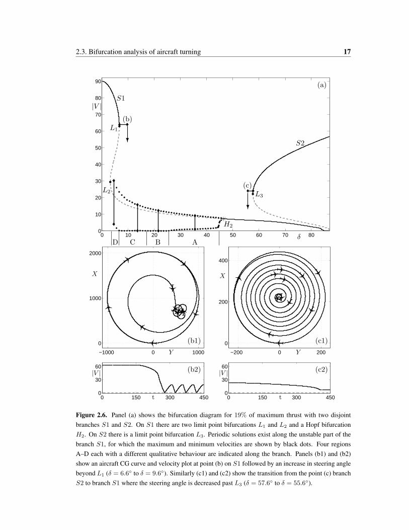
2.3. Bifurcation analysis of aircraft turning 17
.
.
−1000 0 1000
0
1000
2000
0 150 300 4500
30
60
−200 0 200
0
200
400
0 150 300 4500
30
60
0 10 20 30 40 50 60 70 800
10
20
30
40
50
60
70
80
90
|V |
δ
?
?
(c)
(b)L1
L2L3
H2
(a)
S1
S2
ABCD
X X
(b1) (c1)
Y Y
|V | |V |
t t
(b2) (c2)
Figure 2.6. Panel (a) shows the bifurcation diagram for 19% of maximum thrust with two disjointbranches S1 and S2. On S1 there are two limit point bifurcations L1 and L2 and a Hopf bifurcationH2. On S2 there is a limit point bifurcation L3. Periodic solutions exist along the unstable part of thebranch S1, for which the maximum and minimum velocities are shown by black dots. Four regionsA–D each with a different qualitative behaviour are indicated along the branch. Panels (b1) and (b2)show an aircraft CG curve and velocity plot at point (b) on S1 followed by an increase in steering anglebeyond L1 (δ = 6.6◦ to δ = 9.6◦). Similarly (c1) and (c2) show the transition from the point (c) branchS2 to branch S1 where the steering angle is decreased past L3 (δ = 57.6◦ to δ = 55.6◦).

18 Chapter 2. Bifurcation analysis of turning solutions
sufficient to overcome the holding force generated by the nose gear if the aircraft is in motion.On the stable part of the new branch S2 the aircraft follows a large turning circle solution withthe nose gear tyres saturated.
We now consider the role of the limit point bifurcations L1 and L3. Starting at a solutionon the stable part of the branch S1 and increasing the steering angle just beyond L1 causes theaircraft to move towards a different attractor. At point (b) with the steering angle δ = 6.6◦ theaircraft follows a turning circle with radius r ≈ 1km. When the steering angle is ramped up toδ = 9.6◦ the aircraft moves towards to a different attractor. A CG curve plot and velocity |V |time plot are shown in Figures 2.6(b1) and (b2). In the simulation the aircraft follows a turningcircle until the steering angle is ramped up after 150s to a value beyond L1, then the aircraftspirals inwards towards a periodic solution similar to that shown in Figures 2.5(b1) and (b2).There would be no immediate indication to a pilot that the limit point bifurcation is approachedor passed; the aircraft tends to the periodic solution over a transient period. Decreasing thesteering angle from δ = 9.6◦ (to a value below that at L2) causes the aircraft to deviate fromthis periodic solution and return to following a large turning circle on the stable part of branchS1. These two transitions between the stable part of S1 and the periodic solution existing forvalues of δ along the unstable part of S1 form a hysteresis loop. In the example just describedthe aircraft jumps from a stable part of S1 to a periodic solution about an unstable part of S1.A similar jump, this time between different branches, occurs when starting at a solution on thestable part of the branch S2 and decreasing the steering angle below L3. In this case the aircraftmoves from a stable solution on branch S2 to a stable solution on the branch S1. At point (c)the steering angle is initially δ = 57.6◦ and ramped down after 70s to δ = 55.7◦. Plots ofthe simulations are shown in Figures 2.6(c1) and (c2). The aircraft follows a turning circle ofradius r ≈ 220m and then spirals in towards a turning circle of radius r ≈ 12m.
In Figure 2.6(a) the maximum and minimum velocities of the periodic solutions are shownby dotted black curves. The behaviour for a steering angle just below the bifurcation H2
was shown in Figure 2.5(c1). The same behaviour persists near H2 for the higher thrust casepresented in Figure 2.6(a). As the steering angle is decreased below the bifurcation H2 thesize of oscillations gradually increases. The increase in size of the oscillations corresponds toa greater loss of velocity when the aircraft deviates from the unstable turning circle solution.Figure 2.6(a) shows a steep but apparently smooth increase in the size of oscillations. Thesteepest part of this increase is at δ ≈ 45◦. For δ < 45◦ there are much larger oscillations.The transition between the small and large oscillations becomes sharper as lower thrust casesare considered as in Figure 2.5(a). This can be attributed to the fact that the transition from theexistence of a stable turning circle for δ > H2 to the unstable behaviour between H1 and H2
happens for smaller δ and, therefore, at a higher velocity in the lower thrust case. The largeoscillations are the subject of Section 2.4.
2.3.3 Two-parameter bifurcation diagrams
Having studied the steady-state solutions for two different thrust cases it is desirable to seewhether the behaviour persists at different thrust levels. We consider the solutions for constantthrust levels that correspond to discrete initial forward velocities |Vinit| ∈ (10m/s, 115m/s).Figure 2.7(a) shows a surface plot of steady-state solutions in (δ, |V |, T )-space where T is thepercentage of the maximum thrust of the engines. Figure 2.7(b) shows a corresponding contour

2.4. Different types of periodic solution 19
plot, effectively a top-down view of the surface in the (δ, |V |)-plane. In both plots the loci oflimit point bifurcations are labelled L and L∗ and the locus of Hopf bifurcations is labelledH . The blue part of the surface that lies below the curves L and H represents stable turningsolutions, and the red part above these curves represents unstable turning solutions. Individualsolution branches used to create the surface are shown at regular intervals on the surface bythin black curves. For orientation, the solution branches shown in Figures 2.4(a) and 2.6(a)are highlighted by thick black lines on the surface and labelled C70 and C90, respectively. Inthe contour plot the stability of the contours C70 and C90 is indicated as in Figures 2.4(a)and 2.6(a).
Bifurcations on the individual solution branches correspond to a crossing of a bifurcationlocus curve. The example C70 consists of one piece, corresponding to the branch S1, whichintersects the Hopf bifurcation locus curve H in two places corresponding to the bifurcationsH1 andH2 in Figure 2.4(a). The transition between C70 and C90 is as follows. With increasingthrust levels two limit point bifurcations appear at a cusp point on L. The curve H terminatesat an intersection with L (a Bogdanov-Takens bifurcation [29], not discussed here) and thusthe Hopf bifurcation H1 no longer appears for thrust levels above this intersection. The secondbranch S2 on C90 can be seen in the background of the surface plot; it is clearly seen in thecontour plot in Figure 2.7(b).
The surface plot reveals that for thrust levels greater than at C90 the structure remainsqualitatively the same except that branches S1 and S2 meet on L∗. For thrust levels below theminimal point on H the behaviour is trivial: for all values of δ the solution branches representstable turning circles. Furthermore, for thrust levels above the saddle point on L, at which pointthe bifurcations L1 and L3 meet and vanish, the behaviour is also uniformly stable. Due to therobustness of the structure, the surface in Figure 2.7(a) explains the equilibria dynamics fully.Therefore, by studying the two cases C70 and C90 in detail and using the surface and contourplots, we have described the underlying dynamics dictating the aircraft’s behaviour across theentire range of relevant values in the (δ, T )-plane comprehensively and in a compact manner.
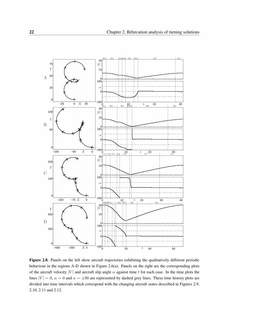
2.4 Different types of periodic solution
We now study the branch of periodic solutions in Figure 2.6(a) for δ ∈ (4.5◦, 46.5◦) in moredetail. An attempt was made to follow the periodic solutions using AUTO, but it was onlypossible to find very short branches near the Hopf bifurcations. Due to the black-box nature ofthe SIMMECHANICS model it is difficult to assess the reason for this computational difficulty,but it may be related to the rapid growth of the solution profile. As an alternative we foundthe periodic solutions by simulation runs for discrete values of the steering angle. The stableperiodic behaviour was found by running the model from an initial state of the system on thestable part of the branch S1 near the bifurcationH2 and ramping down the steering angle. Onceany transient behaviour has passed the persistent behaviour is studied. Here, we focus on theregion the region of large amplitude oscillations (for δ < 44.5◦) which can be divided into foursubintervals that correspond to qualitatively different types of periodic solution. Specificallywe distinguish
case A: δ ∈ (25.5◦, 44.5◦);

20 Chapter 2. Bifurcation analysis of turning solutions
.
.
(a)
|V |
δ
TC90
C90
C70 H
L
L∗
0 10 20 30 40 50 60 70 800
20
40
60
80
100
120
(b)|V |
δ
C90
C90
C70
H
L
L∗
��
���
Figure 2.7. Panel (a) shows the surface of turning solutions in (|V |, δ, T )-space. The loci of limitpoint bifurcations L and L∗ and the locus of Hopf bifurcations H are indicated by a thick lines; theblue part of the surface below H and L consists of stable solutions, and the red part above of unstablesolutions. Individual solution branches used to create the surface are shown at regular intervals as thinblack curves. The solution branches shown in Figures 2.4(a) and 2.6(a) are highlighted by thick blacklines and labelled C70 and C90, respectively. Panel (b) shows a corresponding contour plot of individualcontours in the (|V |, δ)-plane. In the contour plot, the stability of the curves curves C70 and C90 hasbeen indicated as in Figures 2.4(a) and 2.6(a).

2.4. Different types of periodic solution 21
case B: δ ∈ (17.5◦, 25◦);
case C: δ ∈ (7◦, 17◦);
case D: δ ∈ (4.5◦, 6.5◦).
The boundary between the regions A and B is the point where the minimum velocity of theperiodic solution first reaches |V | = 0. Similarly the transition from C to D is associated withthe minimum velocity becoming non-zero again.
Figure 2.8 shows CG curves plotted in the (X,Y )-plane over one period of motion withcorresponding time history plots of the aircraft velocity |V | and the slip angle α. Plottedis the stable behaviour at δ-values that are representative for the four intervals A–D shownin Figure 2.6. Across each region the behaviour is qualitatively the same. The aircraft slipangle gives the aircraft’s orientation relative to its direction of motion. Recall that the slipangle is used to calculate the orientation of the markers on the CG curves. For each of thecases A–D there are common features that can be identified. The data is plotted over oneperiod taken between points of maximum velocity. Therefore, the initial points represent theaircraft approximately following the unstable turning circle but at a slightly higher velocity.The turning circle solution is unstable so the aircraft deviates from it, loses velocity and comesto a near or full stop. The point of minimum velocity corresponds to the point of maximumcurvature on the aircraft CG curve. Due to the constant thrust, the aircraft then speeds up oncemore, approaching the turning circle before again reaching the maximum velocity at the finalpoint. From the plots in the left column a longer trajectory is obtained by repeatedly copyingand translating each trajectory so that the start and final points connect. Figure 2.5(c1) is anexample of what such a trajectory looks like.
The time plots in the right column of Figure 2.8 are divided into numbered time intervalseach representing a qualitative state of the aircraft. Transitions between the intervals indicate aqualitative change. For example, for case A the transition between A3 and A4 corresponds tothe modulus of the aircraft slip angle |α| exceeding 90◦. This means that the aircraft has rotatedbeyond slipping sideways relative to its direction of motion and has a backwards componentto its motion. Clearly it is necessary to look at other features of the aircraft behaviour to fullyexplain all these transitions. Therefore we now introduce a diagrammatic representation thattakes into account many aspects of the aircraft’s behaviour, to give a very detailed account ineach case.
The overall behaviour in regions A–D is as follows. In case A when the aircraft deviatesfrom the unstable turning circle solution it enters a skid and loses velocity until the skid isrecovered and the aircraft starts to approach the unstable turning circle solution again as itspeeds up. In case B the aircraft enters a skid in a similar fashion to case A but skids roundalmost 180◦ and rolls backwards before coming to a complete stop. Case C is similar to B,but now the aircraft skids through 180◦ and briefly follows a backwards turning circle beforestopping. In cases B and C the skid is only recovered when the aircraft comes to a halt. Afterstopping it speeds up again and approaches the unstable turning circle solution. In case D theaircraft enters a skid and makes a full rotation relative to its CG curve without coming to a stop.The skid is only recovered when the aircraft is travelling forwards again.
22 Chapter 2. Bifurcation analysis of turning solutions
.
.
−25 0 25
0
25
50
75
0 10 20 30−180
0
1800
15
30A1 A2 A3A4 A5 A6 A7 A1
X
Y
α
|V |
t
−100 −50 0
0
50
100
0 10 20 30−180
0
1800 10 20 300
15
30B1 B2 B3 B4/5 B6 B1
X
Y
α
|V |
t
−150 −75 0
0
100
200
0 10 20 30 40−180
0
1800 10 20 30 400
15
30C1 C2 C3 C4 C5 C7 C1
X
Y
α
|V |
t
−500 −250 0
0
250
500
0 20 40 600
15
30
0 20 40 60−180
0
180
X
Y
α
|V |
t
D1D2D3 D6 D7 D8 D1
D
C
B
A
Figure 2.8. Panels on the left show aircraft trajectories exhibiting the qualitatively different periodicbehaviour in the regions A-D shown in Figure 2.6(a). Panels on the right are the corresponding plotsof the aircraft velocity |V | and aircraft slip angle α against time t for each case. In the time plots thelines |V | = 0, α = 0 and α = ±90 are represented by dashed grey lines. These time history plots aredivided into time intervals which correspond with the changing aircraft states described in Figures 2.9,2.10, 2.11 and 2.12.

2.4. Different types of periodic solution 23
2.4.1 Diagrammatic representation
Figures 2.9–2.12 each show time plots of the nose tyre slip angle αN and main outer tyre slipangle αM for the cases A–D. We do not distinguish between the behaviour of the inner andouter main gears as both gears act practically simultaneously in the cases studied. The tyreforces are larger on the outer gear due to a greater load. Therefore, the slip angle of the outergear αM is used to represent the behaviour of both the main gears. In the time history plotsof Figures 2.9–2.12 there is a dashed black line indicating the optimal slip angle at which thetyre will generate the greatest holding force. These plots show concurrent information with theplots in Figure 2.8. The plots are divided into numbered regions for which a given aircraft statecan be identified.
For each of the numbered regions in the time plots of Figures 2.9–2.12 there is a corre-sponding diagram at the top of the figure. Each diagram shows several pieces of informationabout the state of the aircraft. Recall that the aircraft markers in the CG curve plots of Fig-ure 2.8 indicate the slip angle of the aircraft, that is, the angle it makes with its direction ofmotion. The direction of motion is indicated in the diagrams in Figures 2.9–2.12 by an arroworiginating from the CG position that is pointing to the left. The slip angle of the aircraft inthe diagrams is indicated schematically as one of the values α = ±10◦,±45◦,±135◦,±170◦.The direction of rotation of the aircraft, taken from the sign of the rotational velocity of theaircraft, relative to the CG curve is shown about a representative centre of rotation; it may bein front of the nose gear, between the nose and main gears, or behind the main gears. The(approximate) location of the three landing gears is represented by two black tyres, the noseand outer main gear, and a grey tyre, the inner main gear. Recall that we consider the maingears to act simultaneously and therefore only represent the behaviour at the outer gear. Thedirections of tyre forces are shown on the nose gear and main outer gear. From each of thenose and main outer gears originates a double arrow indicating the direction of the tyre force asdetermined by the sign of the tyre slip angles αN,M . Passing through the lines αN,M = 0◦ orαN,M = ±180◦ indicates that the direction of the tyre force changes. The size of these arrowsis uniform, and does not indicate the magnitude of the forces. Finally, a single arrow is shownopposing the tyre force direction if that particular tyre is skidding. In general, when the tyresare rolling and generating a holding force sufficient to control the aircraft the slip angles willchange gradually. A tyre is identified as skidding if the slip angle crosses through the optimalholding force line and the slip angle starts to change rapidly. A tyre is identified as havingrecovered from skidding when the time derivative of its slip angle returns towards 0 (the slipangle curve plateaus out).
2.4.2 Detailed discussion of cases A–D
We now discuss the aircraft dynamics for the cases A–D. After a brief summary each peri-odic state of the aircraft is explained in detail. The reader will find it useful to refer back toFigure 2.8.
Case A: δ ∈ (25.5◦, 44.5◦); as shown in Figure 2.9. Initially the aircraft is at the maximumvelocity and has started to deviate from the unstable turning circle solution; the velocity thendrops as the main tyres start skidding. The aircraft continues to slow down. The skid is re-covered when the aircraft reaches its minimum velocity. The aircraft approximately follows aturning circle as it speeds up from the minimum velocity. In more detail:

24 Chapter 2. Bifurcation analysis of turning solutions
.
.
A1 A2 A3
A4 A5 A6 A7
0 10 20 30−180
0
180−180
0
180
t
αM
αN
A1 A2 A3 A4 A5 A6 A7 A1
Figure 2.9. Diagrammatic representation of the periodic behaviour of the aircraft for region A in Fig-ure 2.6. The two panels show the nose tyre slip angle αN and main tyre slip angle αM over one period(black curves). The optimal slip angle values are shown by dashed black lines. The line αN,M = 0is shown as a dashed grey line. Each aircraft diagram represents the aircraft’s state over the numberedtime intervals on the time history panels.

2.4. Different types of periodic solution 25
A1 The aircraft approximately follows the unstable turning circle solution, held by tyre forces;i.e. it rotates clockwise about a point in front of the nose gear and the aircraft slip angleα is small. The aircraft slip angle α increases as the aircraft gains velocity and graduallystarts to oversteer.
A2 The main tyres saturate (in quick succession, inner followed by outer) and start to skid.The main tyre slip angle αM passes through the optimal slip angle line after which itsslope increases rapidly. The aircraft begins to oversteer excessively and the aircraft slipangle α changes rapidly, the rotational velocity of the aircraft increases.
A3 The main gears continue to skid. The force on the nose gear switches (αN changes sign)to oppose the rotation of the aircraft causing the rotational velocity to fall.
A4 As A3 but the slip angle exceeds |α| > 90◦ (see Figure 2.8) — the aircraft moves beyondsliding sideways with a slight backward component to the motion. The centre of rotationof the aircraft moves through the nose gear causing a sudden jump in its slip angle αN .
A5 Main tyres regain traction, evidenced by the main tyre slip angle αM plateauing out, soboth the nose tyres and main tyres oppose the spin — effectively bringing the spin undercontrol. The slip angle of the aircraft α plateaus out as it regains control.
A6 The aircraft has stopped skidding and starts to travel forwards again; the slip angle hasfallen below |α| = 90◦ and therefore, there is no backward component to its motion. Itcontinues to slow down towards its minimum velocity. Although the main tyre slip angleαM changes rapidly, it is moving towards the optimal slip angle line and the tyre force isincreasing.
A7 When the aircraft reaches its minimum velocity the sign of αN changes so that the direc-tion of the nose tyre force matches the main gears. The aircraft speeds up and starts tofollow an approximate turning circle. Initially, whilst travelling at low velocity the aircraftundersteers slightly before starting to oversteer at the transition back into A1.
Note: For δ ∈ (40.5◦, 44.5◦) in case A the aircraft slip angle does not exceed |α| > 90◦ and inthis case the steps A4 and A5 do not occur in Figure 2.9.
Case B: δ ∈ (17.5◦, 25◦); as shown in Figure 2.10. The aircraft enters a skid in a similar wayto case A but does not recover from the skid. The aircraft skids round almost 180◦ and onlystops skidding when the tyres are rolling backwards. The aircraft rolls backwards, oscillatingfrom side to side with a slip angle just greater than α = −180◦. The constant forward thrustbrings the aircraft to a halt, the slip angle α passes through α = −180◦ to become positive andreturns rapidly towards α ≈ 0◦ as the aircraft starts moving forwards again. The significantdifference with case A is that the aircraft makes a full rotation relative to the CG curve and alsothat the aircraft comes to a complete halt (|V | = 0). After coming to a halt it starts to move offagain following an approximate turning circle. In more detail:
B1 As A1.
B2 As A2.

26 Chapter 2. Bifurcation analysis of turning solutions
.
.
B1 B2 B3
B4 B5 B6
0 10 20 30−180
0
180−180
0
180
t
αM
αN
B1 B2 B3 B4/5 B6 B1
Figure 2.10. Diagrammatic representation of the periodic behaviour of the aircraft for region B asshown in Figure 2.6. The two panels show the nose tyre slip angle αN and main tyre slip angle αM
over one period (black curves). The optimal slip angle values are shown by dashed black lines. The lineαN,M = 0 is shown as a dashed grey line. Each aircraft diagram represents the plane’s state over thenumbered time intervals on the time history panels.

2.4. Different types of periodic solution 27
B3 The direction of the force on the nose gear changes as the aircraft starts to rotate about apoint between the nose and main gears. Simultaneously the slip angle exceeds |α| > 90◦.Qualitatively the same as A4, effectively missing out A3 because the aircraft rotatesfaster in the skid.
B4/5 The aircraft skids round far enough such that the tyres regain traction whilst rollingbackwards. The aircraft slip angle α plateaus out into a region of small oscillations justabove α = −180◦. As the aircraft travels backwards the momentum from the skid causesit to roll from side to side (the wings pitch up and down). The forces on the main tyresswitch from side to side and the direction of rotation alternates, switching between B4and B5. As the aircraft is travelling backwards the constant thrust rapidly slows it down,bringing it to a complete halt. The slip angle passes through α = −180◦, becomingpositive and rapidly returning towards α = 0◦.
B6 The aircraft moves off from stationary following an approximate turning circle; as A7.
Case C: δ ∈ (7◦, 17◦); as shown in Figure 2.11. The aircraft enters a skid in a similar fashion tocases A and B, but it skids over 180◦ before the tyres stop skidding. The aircraft briefly followsa backwards turning circle whilst the forward thrust slows it down. Although the translationalvelocity reaches |V | = 0, it still has rotational velocity at that point. The significant differencefrom case B is that the aircraft tyres regain traction after it has spun over 180◦, i.e. the slipangle has passed through α = −180◦. The momentum from the skid maintains a rotationalvelocity when the aircraft travels backwards. After stopping (translationally, not rotationally)the aircraft then moves off following a turning circle in the forward direction. In more detail:
C1 As A1 and B1.
C2 As A2 and B2.
C3 The aircraft has more momentum as, in this case, the velocity is higher when the aircraftenters a skid. Traction on the main and nose tyres is lost before the aircraft slides pastα = 90◦. In contrast to the previous cases, all tyres are skidding. The slope of the aircraftslip angle α increases.
C4 The direction of the force on the nose tyre switches and the centre of rotation moves to aposition between the main and nose gears. All the tyres oppose the direction of rotationbut are skidding. The aircraft slip angle α continues to changes rapidly.
C5 The aircraft slip angle moves through α = −180◦ after which the main tyres and the nosetyres regain traction. The aircraft follows a backwards turning circle with a small, almostconstant aircraft slip angle α. The main tyre slip angle αM remains very small and doeschange sign once (although this is not indicated in the diagram).
C6 The aircraft (translational) velocity reaches |V | = 0 instantaneously but as it passes throughthis point it still has rotational velocity. The momentum of the aircraft causes it to carryon rotating in the same direction as it travels backwards. The aircraft starts to accelerateagain, moving in a forward direction, due to the constant thrust.
C7 As A7 and B6.

28 Chapter 2. Bifurcation analysis of turning solutions
.
.
C1 C2 C3
C4 C5 C6 C7
0 10 20 30 40−180
0
180−180
0
180
t
αM
αN
C1 C2 C3 C4 C5 C7 C1
Figure 2.11. Diagrammatic representation of the periodic behaviour of the aircraft for region C asshown in Figure 2.6. The two panels show nose tyre slip angle αN and main tyre slip angle αM overone period (black curves). The optimal slip angle values are shown by dashed black lines. The lineαN,M = 0 is shown as a dashed grey line. Each aircraft diagram represents the plane’s state over thenumbered time intervals on the time history panels.

2.4. Different types of periodic solution 29
.
.
D1 D2 D3 D4
D5 D6 D7 D8
0 15 30 45 60−180
0
180−180
0
180
t
αM
αN
D1 D2 D3 D6 D7 D8 D1
Figure 2.12. Diagrammatic representation of the periodic behaviour of the aircraft for region D asshown in Figure 2.6. The two panels show the nose tyre slip angle αN and main tyre slip angle αM
over one period (black curves). The optimal slip angle values are shown by dashed black lines. The lineαN,M = 0 is shown as a dashed grey line. Each aircraft diagram represents the plane’s state over thenumbered time intervals on the time history panels.

30 Chapter 2. Bifurcation analysis of turning solutions
Case D: δ ∈ (4.5◦, 6.5◦); as shown in Figure 2.12. The aircraft enters a skid at a highervelocity than the previous cases. The aircraft has more momentum, so that it makes a full 360◦
spin relative to the CG curve before traction on the tyres is regained. In contrast to the previoustwo cases, when the aircraft travels backwards the tyres continue skidding. Once the aircraft isfacing forwards after the spin it has lost sufficient momentum for the tyres to stop skidding andthe aircraft returns to following an approximate turning circle. In more detail:
D1 As A1, B1 and C1.
D2 As A2, B2 and C2.
D3 As C3.
D4 The aircraft continues to skid, the slip angle exceeding α = 90◦ before direction of theforce on the nose gear changes. The centre of rotation stays at a point in front of the nosegear.
D5 As C4.
D6 The aircraft spins through α = 180◦, the tyres not regaining traction. The force on themain tyres changes direction and the aircraft now spins about a point behind the maingears.
D7 The aircraft continues to rotate and return towards facing forwards whilst slowing to a lowvelocity.
D8 As the aircraft returns to travelling in a forward direction (α ≈ 0) the tyres regain tractionand the aircraft speeds up following a turning circle; as A7, B6 and C7.
Cases A–D above provide a complete explanation of the behaviour when lateral stabilityof the aircraft is lost. From case to case the velocity at which lateral stability is lost increases.Therefore, more momentum is available so that aircraft undergoes a larger rotation before thetyres regain traction. The level of detail shown in our new diagrammatic representation isnecessary in order to fully explain the different types of periodic behaviour and the transitionsbetween them.
2.5 Discussion
A bifurcation analysis of the turning manoeuvres of an Airbus A320 on the ground was pre-sented. Focusing on a particular aircraft configuration, the stability of turning circle solutionswas computed over the entire range of relevant values of steering angle and thrust. It is thestability of these turning circle solutions that dictates whether a particular turning manoeuvreat specific parameter values is laterally stable. The results were rendered as a surface plot,which was constructed from continuation runs with varying steering angle δ at discrete fixedthrust levels. The modulus of the velocity of the aircraft |V | was used in this representation,meaning that the surface is represented in (δ, |V |, T )-space. We found that the single param-eter continuation curves corresponding to fixed thrust levels are qualitatively the same over

2.5. Discussion 31
large ranges of thrust. Due to this robustness in the structure of the surface it was possible tofully explain the dynamics represented on the surface by studying two individual thrust casesin detail. These two cases were explained in terms of the solutions represented by the bifurca-tion diagrams. Examples were given of branch switching near limit point bifurcations and ofthe periodic solutions that arise from Hopf bifurcations. In this way two significant types ofbehaviour were identified: stable turning circle solutions and periodic solutions for which theaircraft loses lateral stability, entering a skid or even a spin.
As an example of how bifurcation analysis can uncover even quite subtle effects of practicalinterest, we consider the dynamics near the limit point L1 in Figure 2.6(a). On the stablebranch close to L1, a small increase in the steering angle beyond the bifurcation leads to atransition to the low-velocity part of the solution branch. In this case the aircraft moves toa laterally unstable behaviour over a transient period. It is not immediately obvious how torelate this observation to inherent properties of the aircraft system that could be monitored. Athigh velocity the aerodynamic forces generated by the aircraft’s vertical tail attempt to keepthe aircraft travelling in a straight line. As the steering angle is increased and the limit pointis approached two things happen. The turning moment generated by the nose gear tyres isincreasing and the aerodynamic holding force decreases (with the aircraft velocity). The limitpoint corresponds to the aerodynamic holding force being overcome by the turning momentgenerated at the nose gear. This observation shows that bifurcation analysis can reveal featuresof the dynamics that otherwise would not be immediately evident.
In conjunction with the bifurcation analysis, model simulations were used to study periodicorbits in the region of unstable turning solutions. A detailed explanation of the dynamicswas given by means of a diagrammatic representation of changing states of the aircraft. Thefocus was on attributing qualitative changes in the behaviour under parameter variation to thesaturation of the forces generated by individual tyres. Four regions of qualitatively differentbehaviour were identified, and the differences and transitions between them explained. Thediagrammatic explanation gave details of the undesirable behaviour when the aircraft loseslateral stability. The safe operating limits that avoid this behaviour, have been identified overthe relevant ranges of steering angle and thrust by the bifurcation analysis. Specifically, ourresults identify that for high-velocity turns, such as when exiting the runway, maintaining asteering angle below δ = 3.5◦ ensures lateral stability. This value agrees with empirical data,and it is used in the A320’s steering system as a limit for high-velocity turns. Furthermore,a curve of Hopf bifurcations in the steering angle versus thrust parameter space is identifiedas the boundary for lateral stability (safe operation) when performing manoeuvres at lowervelocities.


Chapter 3
Operational parameter study
The model and results presented in Sections 3.2, 3.3 and 3.4 have been published in [44]; theresults in Section 3.5 appeared in [43].
3.1 Introduction
In this chapter we develop a fully parameterized, mathematical model of an aircraft turningon the ground; effectively, the full equations of motion for the model outlined in Chapter 2 aregiven. We demonstrate that the new model allows us to extend previous work with a bifurcationstudy in terms of several operational parameters. The new mathematical model takes the formof a system of coupled ordinary differential equations (ODEs). The airframe is considered asa rigid body with six DOF and the equations of motion are derived by balancing the respec-tive forces and moments. Specific sub-components are modelled in accordance with industryexperience and test data, and nonlinear effects are included in the models of the tyres and theaerodynamics. In this way, the overall mathematical model incorporates an appropriate levelof complexity. This new mathematical model provides several advantages over the existingSIMMECHANICS model used in Chapter 2, especially when used with continuation software.Its general functionality and computational efficiency with the software package AUTO is dra-matically improved. Furthermore, the model does not suffer from a black-box nature, whichmeans that all variables and parameters — both design parameters (such as dimensions of theaircraft) and operational parameters (such as total mass and CG position) — are fully accessi-ble.
The development of the mathematical model was guided by the SIMMECHANICS modeldescribed in Section 2.2. Following the implementation of the mathematical model, the firstgoal was its validation via a direct comparison with existing results from Chapter 2. The vali-dation is demonstrated with a one-parameter bifurcation analysis that focuses on the agreementbetween different types of solutions in each model. In particular, stable turns and periodic solu-tions for which the aircraft loses lateral stability are studied. The solutions are presented acrossthe full range of the steering angle for a particular aircraft setup, allowing for a comprehensivecomparison between the models.
We then present an extensive bifurcation analysis of turning solutions of the aircraft undervariation of several operational parameters. One-parameter continuation runs are computed in
33

34 Chapter 3. Operational parameter study
the steering angle at many discrete values of the CG position (over a suitable range). Two-parameter continuation is used to follow curves of bifurcation points directly to determineregions where turning is unstable. As in Chapter 2, the results are represented as surfacesof solutions that describe the possible dynamics over the full range of the two parameters,the steering angle and the centre of gravity position. Moreover, we find that a curve of limitpoint bifurcations forms a fold in the surface of solutions; crossing this curve in parameterspace results in a significant change in the radius of the turning circle that the aircraft attemptsto follow. In contrast with Chapter 2 we find closed curves of Hopf bifurcations; however,these curves still bound regions of unstable turning solutions for which the aircraft followsa laterally unstable motion relative to the unstable turning solution. The robustness of theseresults is further investigated under the variation of the aircraft mass and the thrust level. Wefind that quite small changes in thrust result in a sequence of qualitative changes of the solutionsurface. This occurs for two different mass cases (heavy and light aircraft) but at differentthrust levels. Overall, a heavier aircraft will make stable turns over a larger range of centre ofgravity positions and at higher thrust levels. We also find that the region of laterally unstablebehaviour grows more rapidly with increased thrust for a lighter aircraft.
An investigation into differences in taxiway surface conditions reveals an interesting rela-tion to the results in Chapter 2. We find that reducing the coefficient of friction of the tyreshas the same qualitative effect as increasing the thrust level. This is shown by the qualitativeagreement between surfaces of solutions computed in terms of the two parameters. We arefurther able to elaborate on results presented in Chapter 2 with a detailed investigation of theapparent jump in the amplitude of oscillations that was found to occur close to a Hopf bifur-cation. An advantage of the mathematical model is that we are able to compute branches ofperiodic solutions directly (instead of with time history simulation). With a combination ofdifferent continuation computations and time history simulations we are able to provide a the-oretical explanation for the sharp increase in oscillation amplitude and gain further insight intothe mechanism through which the lateral stability of the aircraft is lost.
The chapter is organised as follows: In Section 3.2 full details of the new model are given.Its validation against the existing SIMMECHANICS model is demonstrated in Section 3.3. Anextensive bifurcation analysis in several parameters is the subject of Section 3.4. The effectof reducing tyre friction is investigated in Section 3.5. In Section 3.6 a sharp increase in theamplitude of periodic oscillations close to a Hopf bifurcation is discussed. Finally, conclusionsand directions of future work are presented in Section 3.7.
3.2 Mathematical model
In this section we give details of the derivation and implementation of a fully parameterizedmathematical model that describes an aircraft moving on the ground. As in Chapter 2 thechosen parameter values and component models represent an A320, however, the model pa-rameters could easily be adapted to represent almost any passenger aircraft. We give a fulldescription of the mathematical model in this chapter; it is effectively a fully parameterizedmathematical version of the SIMMECHANICS model. Therefore, to keep this chapter self-contained, there is some repetition from Section 2.2. Motivations for its development are: toovercome the black-box nature of a model written in SIMMECHANICS (especially concern-ing full access to relevant system parameters), to improve functionality with the continuation

3.2. Mathematical model 35
.
.
.
.������������������������
������������������������
������������������������
������������������������
����������������������������������������������������������������
��������
������
������
������������������������������������������
��������
����������
������������
������������
�������
���������������
������������������
������������������
��������
��������
��������
������
������
��������
������
������
lxR
lyT
lxN
lxT
lxA
lxL
lyR
lyL FyL
FyR
FxL
FxR
x
y
FxNδ
FyN
FxTL
FxTR
MzA
FyA
FxA
.
.����������������
������������������������
��������������
������
����������������
�������
�������
��������
��������������
������
������
������
������
�������
�����
������
lyR lyL
lzN lzLlzR
lzA
lzT
lyT
y
z
FzW
FzR FzNFzL
FyR FyN FyL
FzA
FyA
MxA
.
.
��������
��������
��������
��������
������
������
����������
����������
������������������������
������������������������
����������������
����������������
��������������
������
��������������������������������������������
������
��������
��������������
������������������������������������������
����������
��������
�������������� ��������
������
lxNlxL,R
lzL,R lzN
lzT
lzA
lxA
lxT
FzR
FzL
FxRFxL
FzW
x
z
FxN
FzN
MyA
FzA
FxA
(a)
(b)
(c)
Figure 3.1. Schematic diagram showing relative positions of force elements F∗ acting on the airframewith dimensions defined by l∗ in Table 3.1. Three projections are shown in the aircraft’s body coordinatesystem: the (x, z)-plane in panel (a), the (x, y)-plane in panel (b), and the (y, z)-plane in panel (c). Thecentre of gravity position is represented by a checkered circle, the aerodynamic centre by a white circleand the thrust centre of each engine by a white square.

36 Chapter 3. Operational parameter study
package AUTO [12], and to increase the computational efficiency so that more elaborate bi-furcation studies become feasible. The mathematical model has been derived via force andmoment equations, coupled to relevant subsystem descriptions. It has been fully validatedagainst the existing SIMMECHANICS model; see Section 3.3.
The aircraft modelled here has a tricycle configuration in which the nose gear is used forsteering. We model the aircraft as a single rigid body with DOF; three translational DOF andthree rotational DOF. On the aircraft there are two tyres per gear. Due to the small separationdistance they can be assumed to act in unison and, hence, are described as a single tyre in themodel. We do not include oleos in the model presented here, that is, we assume the landinggears to be rigid. The reason for this simplifying assumption is that oleo dynamics are notexcited in turning as considered in the bifurcation study in Section 3.4. Oleos could be includedinto the model, but at the expense of increasing its dimensionality.
Throughout this study we use one of the conventionally accepted coordinate systems foraircraft. Specifically, the positive x-axis points along the centre-line of the fuselage toward thenose of the aircraft, the z-axis is toward the ground and the y-axis completes the right-handedbody-fixed coordinate system. This body coordinate system is assumed to coincide with theaircraft’s principal axes of inertia, a reasonable assumption due to symmetries of the airframe.The equations of motion were derived from Newton’s Second Law by balancing either theforces or moments in each degree of freedom [14].
In Figure 3.1 the relative positions and directions of the force elements that act on theaircraft are shown in the three standard projections. These diagrams illustrate how the equationsof motion are derived by the balancing of force elements along each axis and moment elementsabout each axis. The equations of motion for the velocities in the body coordinate system ofthe aircraft are given as six ordinary differential equations (ODEs):
m(Vx + VzWy − VyWz) = FxTL + FxTR − FxR − FxL − FxN cos(δ)− (3.1)
FyN sin(δ)− FxA + FzW sin(θ),
m(Vy + VxWz − VzWx) = FyR + FyL + FyN cos(δ)− FxN sin(δ)+ (3.2)
FyA + FzW sin(φ),
m(Vz + VyWx − VxWy) = FzW cos(θ) cos(φ)− FzR − FzL − FzN − FzA, (3.3)
IxxWx − (Iyy − Izz)WyWz = lyLFzL − lyRFzR − lzLFyL − lzRFyR− (3.4)
lzNFyN cos(δ) + lzNFxN sin(δ) + lzAFyA +MxA,
IyyWy − (Izz − Ixx)WxWz = lxNFzN − lzNFxN cos(δ)− lzNFyN sin(δ)− (3.5)
lxRFzR − lzRFxR − lxLFzL − lzLFxL+lzTFxTL + lzTFxTR + lzAFxA + lxAFzA +MyA,
IzzWz − (Ixx − Iyy)WxWy = lyRFxR − lyLFxL − lxRFyR − lxLFyL+ (3.6)
lxNFyN cos(δ)− lxNFxN sin(δ) + lxAFyA+lyTFxTL − lyTFxTR +MzA.
Here a dot notation is used to show the first derivative with respect to time of these states. Thedimensions l∗, given in Table 3.1, are defined in terms of the centre of gravity position whichis parameterized as CG. The parameter CG is defined as a percentage measured along the

3.2. Mathematical model 37
mean aerodynamic chord lmac, taken from the leading edge. The aircraft mass m as definedfor two cases presented in the bifurcation analysis is given in Table 3.1; corresponding valuesof the principal moments of inertia Ixx, Iyy and Izz are used in the model. The velocities alongeach of the aircraft’s axes are given by (Vx, Vy, Vz) and the rotational velocities about the axesby (Wx,Wy,Wz). The weight of the aircraft acting at the centre of gravity (CG) position isdenoted FzW = mg; it is assumed to act along the z-axis in the aircraft body coordinate systembecause the pitch and roll angles remain relatively small throughout this analysis. The steeringangle applied to the nose gear, defined in degrees, is denoted δ. It is used as a parameter inthe bifurcation analysis. The modelling of tyre forces is discussed in Section 3.2.1 and theorthogonal force elements on each of the tyres are denoted Fx∗, Fy∗ and Fz∗, where ∗ indicatesthe nose (N ), main right (R) or main left (L) landing gear. The modelling of the aerodynamicsis discussed in Section 3.2.2. The individual aerodynamic force and moment elements aredefined with respect to the aerodynamic centre of the aircraft and are denoted (FxA, FyA, FzA)and (MxA,MyA,MzA), respectively. The thrust forces are assumed to act parallel to the x-axisof the aircraft and are denoted FxTL and FxTR; the total thrust force from both of the enginesis parameterized as T which is defined as a percentage of the maximum available thrust.
The states that vary most significantly during the aircraft’s motion are the velocity Vx inthe x-direction, the velocity Vy in the y-direction, and the angular velocity Wz about the z-axis (yaw velocity); they are calculated from equations (3.1), (3.2) and (3.6), respectively. Areasonable approximation of the aircraft’s dynamics is given by these three equations alone.However, to calculate the asymmetric loading on the landing gears dynamically and with ahigh level of accuracy it is necessary to solve the equations in the other degrees of freedom: thevertical velocity Vz , angular velocity Wx about the x-axis (roll velocity) and angular velocityWy about the y-axis (pitch velocity) given by equations (3.3), (3.4) and (3.5), respectively.
To calculate the position of the aircraft as it moves over the ground plane it is necessary todo so with reference to a fixed location and orientation in space. Therefore, we solve a set ofequations describing the position of the aircraft in the world coordinate system with position(X,Y, Z) and angular orientation given by the Euler angles (ψ, θ, φ), where ψ is the yaw angle,θ the pitch angle and φ the roll angle. The plane given by Z = 0 is the (flat) ground plane.Transformations between the body coordinate system and the world coordinate system can beperformed by applying the standard sequence of rotations given in Phillips [41]. Defining thevelocities in the world axis as VxW , VyW and VzW , the velocity transformation equations aregiven by: VxW
VyWVzW
=
CθCψ SφSθCψ − CφSψ CφSθCψ + SφSψCθSψ SφSθSψ + CφCψ CφSθSψ − SφCψ−Sθ SφCθ CφCθ
VxVyVz
, (3.7)
where C∗ = cos(∗) and S∗ = sin(∗) for notational convenience. Defining the angular veloci-ties in the world axis as WxW , WyW and WzW , the angular velocity transformation equationsare given by: WxW
WyW
WzW
=
1 SφSθ/Cθ CφSθ/Cθ0 Cφ −Sφ0 Sφ/Cθ Cφ/Cθ
Wx
Wy
Wz
. (3.8)

38 Chapter 3. Operational parameter study
Table 3.1. System parameters and their values as used in the model.
Symbol Parameter ValueDimensions relative to CG position
lxN x-distance to the nose gear (10.186 + CG÷ 100× lmac) mlzN z-distance to the nose gear 2.932 mlxR,L x-distance to the main gears (2.498− CG÷ 100× lmac )mlyR,L y-distance to the main gears 3.795 mlzR,L z-distance to the main gears 2.932 mlxA x-distance to the aerodynamic centre ([0.25− CG÷ 100]× lmac)mlzA z-distance to the aerodynamic centre 0.988 mlxT x-distance to the thrust centre ([0.25− CG÷ 100]× lmac)m
lyTR,TL y-distance to the thrust centre 5.755 mlzT z-distance to the thrust centre 1.229 m
Mass Light case Heavy casem Mass of the aircraft 45420 kg 75900 kg
Tyre parameterskzN Stiffness coeff. of the nose tyre 1190 kN/mkzM Stiffness coeff. of the main tyre 2777 kN/mczN Damping coeff. of the nose tyre 1000 Ns/mczM Damping coeff. of the main tyre 2886 Ns/mµR Rolling resistance coeff. 0.02
Aerodynamics parameterslmac Mean aerodynamic chord 4.194 mSw Wing surface area 122.4 m2
ρ Density of air 1.225 kg/m3
Therefore the equations for the position of the aircraft are given by:
X = VxW , ψ = WzW ,
Y = VyW , θ = WyW ,
Z = VzW , φ = WxW .
(3.9)
The position (X,Y ) and orientation ψ are used to plot trajectories of the aircraft motion. Theheight Z above the ground plane and the angles θ and φ that the aircraft makes with the groundplane are used to calculate the load distribution between landing gears.
3.2.1 Tyre modelling
The force elements acting on the tyres are calculated with a tyre model developed by a GAR-TEUR action group investigating ground dynamics [20]. The fundamental work behind thismodel can be found in [40]. The GARTEUR tyre model was also implemented in the SIM-MECHANICS model, see Section 2.2.1. In order to calculate tyre forces for the mathematicalmodel it is necessary to calculate the local displacements and velocities of the tyres; full details

3.2. Mathematical model 39
are given in this section. The focus of this work is primarily stable turning solutions wheretyre velocities are not small; the tyre model we use is suitable for this application. To ensurethat the tyre model response is always continuous we work under the assumption that as thetranslation velocities of the tyres goes to 0, so do the lateral and longitudinal tyre forces. Thereare models that give more reliable results at low velocities [49, 51]; these models are moreapplicable if the emphasis of the work is on low-velocity operations. Throughout this sectiona second subscript N , L or R following x, y or z indicates that the respective velocity or forceis aligned with the local tyre coordinate system; in the case of the nose gear the componentsxN and yN are not aligned with the body-fixed coordinate system (except when δ = 0◦). Themodel used here assumes that the roll axis of the tyre is always parallel to the ground becausethe pitch and roll angles of the aircraft remain relatively small. It is therefore appropriate to usethe velocities of the aircraft in the body coordinate system and Euler angles to calculate localdisplacements and velocities of the tyres. This section focuses on these calculations that areused in obtaining the tyre forces.
To model the vertical force component on the tyre a linear spring and damper system canbe used [6]. For example, the total force acting on the nose gear is:
FzN = −kzNδzN − czNVzN (3.10)
where VzN is the vertical velocity of the nose gear tyre, and δzN is the nose gear tyre deflectionrepresenting the change in tyre diameter between the loaded and unloaded condition. Thestiffness coefficients kz∗ and damping coefficient cz∗ are specified in Table 3.1. Differences inthe vertical velocity and deflection of each tyre give the asymmetric load distribution betweenthe gears. The vertical velocity of each tyre can be calculated in terms of the velocities in thebody coordinate system as:
VzN = Vz − lxNWy, (3.11)
VzR = Vz + lyRWx + lxRWy,
VzL = Vz − lyLWx + lxLWy,
where Vz∗ is the local vertical velocity of the respective tyre. Due to the assumptions that theroll axes of the tyres remain parallel to the ground and that the pitch and roll angles of theaircraft remain small, the deflection of each tyre is given in terms of the aircraft’s positionstates in the world coordinate system as:
δzN = −lzN − Z + lxNθ, (3.12)
δzR = −lzR − Z − lxRθ − lyRφ,
δzL = −lzL − Z − lxLθ + lyLφ.
The longitudinal and lateral forces at the tyre-ground interface depend on the vertical loadacting on the tyre and on its slip angle. The slip angle of a tyre is the angle the tyre makeswith its direction of motion. For each respective tyre, the slip angle α∗ is defined in terms ofits local longitudinal velocity Vx∗ and its local lateral velocity Vy∗ as:
α∗ = arctan(Vy∗Vx∗
). (3.13)

40 Chapter 3. Operational parameter study
.
.0 30 60 90
Fymax
Fy
αopt α
(αopt, Fymax)
Figure 3.2. Lateral force Fy plotted against slip angle α as calculated from Equation (3.16). Themaximum point Fymax that can be generated by the tyre occurs at the ‘optimal’ slip angle αopt.
Therefore, to find the slip angle it is necessary to find the longitudinal and lateral velocityof each tyre. These velocities are calculated in terms of the aircraft’s velocities in the bodycoordinate system and the steering angle applied to the nose gear δ as:
VxN = Vx cos(δ) + (Vy + lxNWz) sin(δ),VyN = (Vy + lxNWz) cos(δ)− Vx sin(δ),VxR = Vx − lyRWz, (3.14)
VyR = Vy − lxRWz,
VxL = Vx + lyLWz,
VyL = Vy − lxLWz.
Note that the rotational velocities Wx and Wy are considered to be sufficiently small withrespect to Wz that they can be ignored here.
Longitudinal forces on the tyres are due to the rolling resistance force caused by hysteresisin the rubber of the tyre. The pressure in the leading half of the contact patch is higher than inthe trailing half, and consequently the resultant vertical force does not act through the middleof the wheel. A horizontal force in the opposite direction of the wheel movement is neededto maintain an equilibrium. This horizontal force is known as the rolling resistance [57]. Theratio of the rolling resistance Fx, to vertical load Fz , on the tyre is known as the coefficient ofrolling resistance µR as given in Table 3.1 [37]. Therefore, the rolling resistance force on therespective tyre Fx∗ is given by
Fx∗ = −µRFz∗ cos(α∗), (3.15)
which incorporates a cosine function to capture two key features. Firstly, the longitudinal forcedrops off to zero when the tyre is moving sideways (α∗ = ±90◦) and secondly, there is a signchange when the direction of motion changes (|α∗| > 90◦). This adaptation to the longitudinaltyre force model in Section 2.2.1 ensures that the forces are well defined for slip angles closeto α∗ = ±90◦.
When no lateral force is applied to a tyre, the wheel moves in the same direction as the

3.2. Mathematical model 41
wheel plane. When a side force is applied, the tyre generates a slip angle α∗ as defined inEquation (3.13). For small slip angles (α∗ < 5◦) the tyre force increases linearly after whichthere is a nonlinear relationship [57]. The lateral force on the respective tyre Fy∗ is a functionof α∗ and can be represented as:
Fy∗(α∗) = 2Fymax∗αopt∗α∗α2opt∗ + α2
∗, (3.16)
where Fymax∗ is the maximum force that the tyre can generate and αopt∗ is the ‘optimal’ slipangle at which this occurs. The parameters Fymax∗ and αopt∗ depend quadratically on thevertical force on the tyre Fz∗ and, hence, change dynamically in the model. The values fornose gear tyres FymaxN and αoptN , and main gear tyres FymaxR,L and αoptR,L are obtainedfrom the equations:
FymaxN = −3.53× 10⁻⁶F 2zN + 8.83× 10⁻¹FzN ,
αoptN = 3.52× 10⁻⁹F 2zN + 2.80× 10⁻⁵FzN + 13.8, (3.17)
FymaxR,L = −7.39× 10⁻⁷F 2zR,L + 5.11× 10⁻¹FzR,L,
αoptR,L = 1.34× 10⁻¹⁰F 2zR,L + 1.06× 10⁻⁵FzR,L + 6.72.
For values of α∗ outside the quadrant of α∗ ∈ (0◦, 90◦), the curve in Figure 3.2 is reflectedappropriately to either represent the tyre rolling backwards or turning in the opposite direc-tion. The extension of Equation (3.16) over the entire range α∗ ∈ (−180◦, 180◦) is shown inFigure 2.2(c) of Section 2.2.1.
3.2.2 Modelling the aerodynamics
The aerodynamic model presented here is the same as the one described in Section 2.2.3.Aerodynamic effects are nonlinear because the forces are proportional to the square of thevelocity of the aircraft. Due to the geometry of the aircraft, the forces also depend nonlinearlyon the angle the it makes with the airflow, the sideslip angle β and on the angle of attack σ.We consider ground manoeuvres, with no incident wind. Hence, the sideslip angle β of theentire aircraft is equal to and interchangeable with its slip angle. The slip angle of the aircraftis defined in the same way as that of the tyres, but this time in terms of the velocities of theentire aircraft: αac = arctan(Vy/Vx). Because we are studying ground manoeuvres, the angleof attack σ remains relatively steady. There are six components to the aerodynamic forces;three translational and three moments. The forces are assumed to act at the aerodynamic centreof the aircraft [14], defined as 25% along the mean aerodynamic chord from its leading edge.The six force elements are given by
FxA = 12ρ|V |
2SwCx(αac, σ), MxA = 12ρ|V |
2SwlmacCl(αac, σ),FyA = 1
2ρ|V |2SwCy(αac, σ), MyA = 1
2ρ|V |2SwlmacCm(αac, σ),
FzA = 12ρ|V |
2SwCz(αac, σ), MzA = 12ρ|V |
2SwlmacCn(αac, σ),(3.18)
where the parameters ρ, Sw and lmac are defined in Table 3.1. The dimensionless coefficientfunctions C∗ depend nonlinearly on αac and σ and are based on wind-tunnel data and resultsfrom computational fluid dynamics. The coefficients used here were obtained from a modeldeveloped by the GARTEUR group [20].

42 Chapter 3. Operational parameter study
.
.
0 15 30 45 60 75 90
−15
0
15
30
45
60
75
90
0 20 40−10
0
10
−200 −100 0
0
100
200
300
Vx
Vx
δVy
L2
H2
L1
L2 L3
L4
H2
δ
X
Y
Wz
Vx
(a)
(b) (c)
(d)
Figure 3.3. Comparison between the mathematical model (3.1)–(3.6) (grey curves) and the SIMME-CHANICS model (black curves). Panel (a) shows one-parameter bifurcation diagrams for varying steer-ing angle δ and fixed CG = 14% and T = 19%. There is a single branch of turning solutions; stableparts are solid and unstable parts are dashed. Changes in stability occur at the bifurcation points L1, L3,L4 and H2. The maximum and minimum forward velocity of a branch of periodic solutions originatingat H2 are also shown. Panel (b) shows the branch of periodic solutions plotted in the (δ, Vy, Vx)-projection; the (grey) surface was computed from the mathematical model and the individual orbits(black closed curves) on the surface were computed with the SIMMECHANICS model. Panel (c) showsa comparison of the individual periodic orbits at δ = 10◦ in the (Wz, Vx)-projection. The correspondingCG trace of the aircraft in the (X,Y ) ground plane is shown in panel (d) with markers indicating theorientation of the aircraft at regular time intervals. In all figures velocities Vx and Vy are measured inm/s, rotational velocity Wz in deg/s, and distances X and Y in m.
3.3 Validation of mathematical model
We now present results that were used as part of the validation process for the mathematicalmodel described in Section 3.2 against the established SIMMECHANICS model [42]. Specif-

3.3. Validation of mathematical model 43
ically, we show in Figure 3.3 a comparison of a one-parameter bifurcation study of turningsolutions as a function of the steering angle δ. Throughout Figure 3.3, solutions for the math-ematical model (3.1)–(3.6) are in grey and those of the SIMMECHANICS model, as shownpreviously in Figure 2.6(a), are in black. This comparison shows that there is a high level ofagreement between the two models over the entire relevant range of δ. Furthermore, a de-tailed comparison of periodic solutions (corresponding to unstable turning) shows that the twomodels also agree closely in terms of laterally unstable behaviour.
Figure 3.3(a) shows a direct comparison of a bifurcation diagram in δ of turning solutionsfor CG = 14% and T = 19%, where the forward velocity of the aircraft Vx is used as ameasure of the solution; the data from the SIMMECHANICS model have been reproduced fromFigure 4 in Reference [42]. A single branch of solutions originates in the top left of the diagramand terminates in the top right; stable parts are solid curves and unstable parts are dashedcurves. Changes in stability occur at the limit point bifurcations L1, L3, L4 and at the Hopfbifurcation point H2. There is a branch of periodic solutions that originates from H2; themaximum and minimum velocities of these solutions are shown as a continuous solid greycurve for the mathematical model (3.1)–(3.6) and as a series of black dots at discrete pointsfor the SIMMECHANICS model. More details of the solutions represented in the bifurcationdiagram and the significance of passing the different bifurcations is discussed in greater detailin Chapter 2.
Overall there is close agreement in Figure 3.3(a) between the bifurcation curves of the twomodels. Any differences are quite small and restricted to certain regions of operation. At theinitial point where δ = 0 the aircraft travels in a straight line. Here the mathematical model hasa velocity of Vx ≈ 87m/s, while the SIMMECHANICS model has a velocity of Vx ≈ 90m/s.This small difference exists on the branch between the initial point and the bifurcation pointL1 along which the solutions represent large radius turning circles. When the steering angleis increased to a value beyond L1 the aircraft will attempt to follow a smaller radius turningcircle at low velocity. Following the solution branch through L1, at which there is a changein stability, we see that the curves computed with the different models agree closely. Alongsection of the solution branch that is approximately horizontal, which represents small radiusturns, the two models remain in almost exact agreement up to the bifurcation L4. A branch ofperiodic solutions originates at the Hopf bifurcation H2 which is the typical behaviour [50].The respective maximum and minimum velocities along the branch of periodic solutions showa high level of agreement; these solutions are discussed in further detail below. Due to an updatein the way longitudinal tyre forces are handled at high slip angles, the limit point bifurcationL4 is detected in the mathematical model, but not in the original SIMMECHANICS model.Nevertheless the two models exhibit qualitatively the same behaviour in this region of thebifurcation diagram. For the large radius solutions along the branch between L3 and the finalpoint in the top right of Figure 3.3(a) the two models show again a slight difference in velocityalong the branch. Furthermore, the limit point bifurcation L3 occurs at a somewhat lower valueof δ in the mathematical model.
Figure 3.3(b) shows the branch of periodic solutions in the (δ, Vy, Vx)-projection, whereVy is the lateral velocity of the aircraft. In a previous study these solutions were studied ingreat detail and four types of qualitatively different behaviour were identified [42]. We showthis data to demonstrate that the two models agree to a high level of detail even in terms ofthe laterally unstable motion that the periodic solutions represent. The periodic solutions form
44 Chapter 3. Operational parameter study
a surface in parameter times phase space. For the mathematical model, it can be computeddirectly by continuation of the periodic solutions from the Hopf bifurcation point H2. For theSIMMECHANICS model, on the other hand, periodic solutions can only be found at discretevalues of δ by numerical simulation. The two models show excellent agreement: the (black)periodic orbits of the SIMMECHANICS model lie almost exactly on the grey surface of periodicsolutions of the mathematical model. Figure 3.3(c) shows a specific periodic orbit in moredetail for δ = 10◦ in the (Vx,Wz)-projection; Wz is the angular velocity of the aircraft aboutits vertical axis. The two periodic orbits indeed agree so closely that the (black) periodic orbitof the SIMMECHANICS model is eclipsed by that of the mathematical model. Figure 3.3(d)shows a trace of the aircraft’s centre of gravity position over one period of its motion in the(X,Y ) ground plane for each of the two models. Markers drawn to scale on the CG traceshow the aircraft’s relative direction of motion at equal time intervals along the trajectory. Thetrajectories computed with the two models agree very closely in the initial section but appearto diverge slightly after a point close to (X,Y ) = (100, 100) where the tangent of the CG tracechanges very quickly. In fact, at this point in the trajectory, where the velocity of the aircraftis very low, the plot exaggerates a very small discrepancy in the amount the aircraft rotates.Either side of this point the trajectories agree very precisely.
In summary of the validation process, the models agree very closely both in terms of theturning circle solutions represented in the bifurcation diagram, as well as the lateral unstableperiodic solutions. The agreement is well within the accuracy of comparisons with actual testdata, so that the mathematical model (3.1)–(3.6) can be used with confidence. In the bifur-cation diagram there were only some small observable differences at high velocities. Thesedifferences occur because the mathematical model does not include the oleos. As we checked,with the oleos included the aircraft assumes a slightly elevated angle of attack that increasesthe lift and, therefore, reduces the loads on the tyres. In turn, this reduces the longitudinal andlateral forces on the tyres and, thus, the aircraft travels faster with the oleos included. Theslight discrepancy in the amount the aircraft rotates at the point of lowest velocity of the peri-odic solution is also due to the fact that the oleos are not included in the mathematical model.Namely, with oleos a slight shift of weight from the inner to the outer gears accounts for agreater rotation as exhibited by the SIMMECHANICS model in Figure 3.3(d). In spite of thesesmall discrepancies, the dynamics of the two models are still sufficiently close and qualita-tively the same over the entire operating range. Furthermore, the close agreement between thetwo models justifies that we do not include the oleos as part of Equations (3.1)–(3.6) for thebifurcation study of turning solutions.
3.4 Two-parameter bifurcation study and sensitivity analysis
In this section we present two-parameter bifurcation diagrams, where we track turning solu-tions in dependence on the steering angle δ and the centre of gravity position CG. By choosingto represent turning solutions in terms of their corresponding forward velocity Vx, we obtain asurface of turning solutions in (δ, Vx, CG)-space. From a practical point of view, this surfaceis assembled from one-parameter continuation runs in δ, as presented in Section 3.3, whichare computed at discrete values of CG that cover an appropriate range. Two-parameter con-tinuation with AUTO is used to compute the loci of limit point and Hopf bifurcations directlyunder the variation of both δ and CG. Combining the results from these two computations into

3.4. Two-parameter bifurcation study and sensitivity analysis 45
a single plot is an effective way of representing the turning dynamics and its stability over thecomplete range of δ and CG in a single figure. What is more, we are able to perform a sensitiv-ity analysis of turning solutions by computing the respective solution surfaces for different fixedvalues of other parameters. Specifically, we consider different thrust cases for a heavy aircraftin Section 3.4.1, and for a light aircraft in Section 3.4.2. Finally, we show two-dimensionalprojections of bifurcation curves to highlight certain features that explain qualitative changesin the bifurcation structure when the thrust is changed.
3.4.1 Heavy aircraft case
Figure 3.4 shows three surfaces of turning solutions in (δ, Vx, CG)-space for the case of aheavy aircraft, each at a different value of the thrust T . Computed solution branches for fixeddiscrete values of CG originate on the left side of the diagram; they are initially stable and maybecome unstable at bifurcation curves on the surface, namely along the curve L of limit pointbifurcations and the curve H of Hopf bifurcations. Note that the typical operating range forthe centre of gravity position is CG ∈ (10%, 40%). Nevertheless, it is convinient to show anextended CG-range to demonstrate completeness of the overall bifurcation structure. To aidin the visualisation of the key bifurcations at small steering angles one-parameter bifurcationdiagrams at fixed CG are shown in Figure 3.5 for the three different thrust cases. Specifically,CG is fixed at 30% and δ is varied as the continuation parameter over the range δ ∈ (0◦, 10◦).The branches are plotted as dashed curves and labelled CG30 in Figure 3.4; their intersectionswith the bifurcation curves L and H correspond to bifurcation points.
In Figure 3.4(a), for a thrust of T = 16% of maximal thrust, we can see that for a forwardCG position of CG < 20% the solutions are uniformly stable. At δ = 0◦ the aircraft travelsin a straight line with Vx ≈ 68m/s; this initial velocity remains constant under variation ofCG. As δ is increased, the velocity of the stable solutions decreases rapidly before startingto plateau out at δ ≈ 7.5◦; the velocity of solutions continues to decrease gradually downto 0m/s as δ is increased towards 90◦. Therefore, for CG < 20% and with increasing δ,there is a continuous and stable transition from stable large radius solutions via stable smallradius solutions all the way to a stationary solution where the nose gear is perpendicular to thedirection of motion. For fixed CG ∈ (20%, 50%) the individual solution branches intersectthe curve of limit point bifurcations L at two bifurcation points. The minimal point on L atCG ≈ 20% is a cusp point [29]. When traversing the surface from left to right (fixing CGbut varying δ) there are fold points in the solution branches that occur at intersections with L.Figure 3.5(a) shows the solution branch CG30 for the case T = 16%. In this one-parametercontinuation the bifurcation points L1 and L2 correspond to intersections on the surface withthe curve of limit point bifurcations L. When the limit point bifurcation curve L is crossedat the left fold in Figure 3.4(a) (corresponding to L1 in Figure 3.5(a)) the large-radius turningsolution becomes unstable and, the aircraft spirals towards and then follows a stable small-radius solution. Similarly, when L is crossed at the right fold in Figure 3.4(a) (correspondingto L2 in Figure 3.5(a)) the small-radius solution becomes unstable and the aircraft spirals outto and settles down onto a stable large-radius solution. Therefore, as is typical in systems withseveral limit point bifurcations, there is a hysteresis loop [19] between large- and small-radiusturns. A similar hysteresis loop exists between large-radius and small-radius solutions underthe variation ofCG at fixed values of δ > 5◦. At large values of δ andCG the solutions that can

46 Chapter 3. Operational parameter study
.
.
CG%
CG30
Vx
δ
L
?
(a)
CG%
CG30
Vx
δ
L
?
H
6
(b)
CG%
CG30
Vx
δ
L
?
H
6
(c)
BT
BT
s
s
Figure 3.4. Surfaces of turning solutions in (δ, Vx, CG)-space for a heavy aircraft (as specified inTable 3.1) and for three fixed values of the thrust; T = 16% in panel (a), T = 18% in panel (b), andT = 20% in panel (c). Stable solutions are black and unstable solutions are grey; limit point bifurcationsoccur along the thick black curve L and Hopf bifurcations occur along the thick grey curveH; the blackdots in panel (c) are Bogdanov-Takens bifurcation points labelled BT . The specific cases plotted inFigure 3.5 are shown as dashed curves and labelled CG30 in each panel.
be seen in the background of the Figure 3.4(a) represent large-radius turns for which the nosegear does not generate enough force to keep the aircraft stationary and is, hence, effectively

3.4. Two-parameter bifurcation study and sensitivity analysis 47
.
.0 2 4 6 8 100
20
40
60
800 2 4 6 8 10
0
20
40
60
800 2 4 6 8 10
0
20
40
60
80
Vx
Vx
Vx
δ
δ
δ
L1
L2
L1
L2
L1
L2
H2
H1H2
(c)
(b)
(a)
Figure 3.5. One-parameter bifurcation curves at fixed CG = 30% for varying δ ∈ (0◦, 10◦) plottedagainst Vx for T = 16% in panel (a), T = 18% in panel (b), and T = 20% in panel (c). Stable solutionsare black and unstable solutions are grey. Limit point bifurcations L1 and L2 are marked with solid dotsand Hopf bifurcations H1 and H2 with stars.
dragged along the ground. For sufficiently large values of CG > 55% the solution branchesbecome uniformly stable, and they represent large-radius turns only.
When the thrust level T is increased, many of the features of the surface described abovepersist, but there are some changes. Figure 3.4(b) shows the surface for T = 18%. Here theforward velocity when δ = 0◦ has increased to Vx ≈ 74m/s. Another change is that the CG-level at which the solution branches first intersect L has decreased to CG ≈ 12%. However,the most significant difference is a qualitative change in the dynamics: a closed curve of Hopfbifurcations now bounds a new region of unstable turning solutions on the surface. This newregion exists for small δ andCG ∈ (29%, 46%). Figure 3.5(b) shows the solution branchCG30
for the case T = 18%. The two limit point bifurcations L1 and L2 persist from the lower thrustcase but have moved further apart both in terms of δ and Vx. There are two new bifurcationsH1

48 Chapter 3. Operational parameter study
and H2 that correspond to intersections on the surface with the curve H of Hopf bifurcations.Crossing H into this region represents a change where the aircraft will attempt to follow aturning circle solution that is unstable and, therefore, it loses lateral stability. An example ofthis type of solution was given in Figure 3.3(c) and (d); an extensive account of qualitativelydifferent types of laterally unstable solution can be found in Reference [42]. Note further thatcrossing L at the left fold may now lead to the aircraft moving from a stable large-radius turnto laterally unstable behaviour. However, for CG < 29% this bifurcation along L does notlead to a loss of lateral stability.
Figure 3.4(c) shows that there is a further qualitative change when the thrust is increasedto T = 20%. Namely, the regions bounded by the curves L and H have increased in size: theminimum point onL occurs now atCG ≈ 5%, andH exists over the rangeCG ∈ (20%, 49%).As a consequence, the regions bounded by the curves L and H have increased in size so muchthat the curve H is no longer closed but terminates at two intersection points with the curveL. Mathematically, these intersection are known as Bogdanov-Takens bifurcation points [29]and labelled BT . Figure 3.5(c) shows the solution branch CG30 for the case T = 20%. Inthis high-thrust case the limit point bifurcations L1 and L2 persist and are further separated.The Hopf bifurcation H1 is no longer encountered above the lower point BT in Figure 3.4(c)while H2 persists and has moved to a larger value of δ. Further details of the topologicalchange associated with the emergence of Bogdanov-Takens bifurcation points are given inSection 3.4.3. Another change is that the value of CG above which the dynamics are uniformlystable is now reduced, from CG ≈ 55% in Figure 3.4(a) to CG ≈ 50% in Figure 3.4(c).
The properties of the solution surfaces in Figure 3.4 have physical interpretations in termsof the dynamics of the aircraft. When CG is increased (the CG position is moved aft) the loadon the nose gear is reduced and, thus, the turning force that it can generate is reduced. Whenmaking high-velocity turns the aerodynamic forces have a greater effect. In fact, at sufficientlyhigh speeds the holding force generated by the tailplane, which attempts to keep the aircrafttravelling in a straight line, becomes more dominant than the turning force generated by thenose gear. This explains why in each panel of Figure 3.4, for a greater value of CG, the leftfold ofLmoves to a larger value of δ because a greater steering angle is required to generate thenecessary turning moment to overcome the aerodynamic holding force. Similarly, the right foldalong L is associated with the effect that a decreasing turning moment from the nose gear (as δis decreased) is being overcome by the aerodynamic forces. Overall, the region bounded by Lgrows with thrust because at higher velocities the aerodynamic forces are increased. The regionbounded by H appears and grows with increasing thrust level because the aircraft attempts tomake higher velocity turns to the point where they become laterally unstable.
3.4.2 Light aircraft case
Figure 3.6 shows surfaces of turning solutions for the case of a light aircraft for three fixedvalues of the thrust. They are represented in the same way as for the heavy case, except thatthe range of CG has been extended to CG ∈ (−20%, 60%). The first result is that the turn-ing behaviour for both loading cases is qualitatively the same in the respective panels for low,medium and high thrust; compare with Figure 3.4. Nevertheless, there are some quantitativedifferences that are of importance from the operational point of view. First of all, notice thatthe thrust levels identified for the light aircraft case are 4% less throughout compared with the

3.4. Two-parameter bifurcation study and sensitivity analysis 49
.
.
CG%
Vx
δ
L
?
(a)
CG%
Vx
δ
L
?
H
6
(b)
CG%
Vx
δ
L
?
H6
(c)
BT
BT
s
s
Figure 3.6. Surfaces of turning solutions in (δ, Vx, CG)-space for a light aircraft (as specified in Ta-ble 3.1) and for three fixed values of the thrust; T = 12% in panel (a), T = 14% in panel (b), andT = 16% in panel (c). Stable solutions are black and unstable solutions are grey; limit point bifurca-tions occur along the thick black curve L and Hopf bifurcations occur along the thick grey curve H; theblack dots in panel (c) are Bogdanov-Takens bifurcation points labelled BT .
heavy case. More specifically, for a value of thrust of T = 12%, as shown in Figure 3.6(a), theinitial velocity at δ = 0◦ on the individual solution branches is Vx ≈ 63m/s. Furthermore, theregion bounded by the curve L for small δ does not extend as far into the operational range ofCG as for the heavy aircraft case; compare with Figure 3.4(a). When the thrust is increased

50 Chapter 3. Operational parameter study
by 2% we again find a region of laterally unstable behaviour, bounded by a closed curve ofHopf bifurcations H; see Figure 3.6(b). However, the size of the instability region boundedby H is dramatically larger when compared to the corresponding heavy aircraft case in Fig-ure 3.4(b). Namely, the minimal point on L has moved to CG ≈ 15% and the region boundedby H extends over the range CG ∈ (1%, 42%), below the minimal point on L. Therefore,in contrast to the heavy case, passing the bifurcation on the left fold along L always resultsin the aircraft settling onto laterally unstable behaviour. Furthermore, the region of laterallyunstable behaviour in Figure 3.4(b) is accessible from the left without passing a limit point bi-furcation. This means that the region of laterally unstable behaviour could be approached moresuddenly at lower velocities. When the thrust in increased further to T = 16%, as is shown inFigure 3.6(c), the regions bounded by L and H increase further and we again find that H endsat two Bogdanov-Takens bifurcation points on L. Furthermore, the minimal point on L movesto a negative value of CG ≈ −1% and the range of H extends to CG ∈ (−18%, 48%). Notethat a negative value of CG represents a CG position in front of the leading edge of the meanaerodynamic chord.
Overall, we find in the light aircraft case that the size of the region of laterally unstablebehaviour increases much more dramatically when compared with the heavy aircraft case. Thisis a quantitative observation that is of relevance in spite of the fact that the respective panelsfor the two loading cases are qualitatively the same. Note however that a higher thrust level (ofan extra 4% of maximal thrust) is required in the heavy case to achieve similar velocities to thelight case. As a result of this the aircraft is much more susceptible to a loss of lateral stabilityin the light case, as is represented by substantially larger regions of laterally unstable turningsolutions.
3.4.3 Qualitative changes of the surfaces of solutions with thrust
In Section 3.4.1 and Section 3.4.2 it was demonstrated that the aircraft shows considerablesensitivity to the thrust level: qualitative changes in the overall solution surface occur withina range of 2% of maximum thrust. We now discuss these qualitative changes in more detail.While the nature of the transitions is the same for both loading cases, we consider here the caseof a light aircraft as presented in Figure 3.6 because it was seen to be more susceptible to a lossof lateral stability when the thrust is increased.
First of all, the qualitative change between panels (a) and (b) of Figure 3.6 is due to thefact that a closed curve, or isola, H of Hopf bifurcations appears at a specific thrust value inthe interval T ∈ (12%, 14%). Indeed, when the thrust is decreased from T = 14% then theisola shrinks to a point and disappears. This type of qualitative change of the curve H is dueto a smooth transition through a minimum in the associated two-dimensional surface of Hopfbifurcations in (δ, CG, T )-space. This happens at a single value of T in this three-dimensionalparameter space, which is why this is referred to as being of codimension three.
The transition between panels (b) and (c) of Figure 3.6, on the other hand, is more com-plicated. As Figure 3.7 shows by means of projections of the bifurcation curves L and H ,it involves the introduction of two Bogdanov-Takens bifurcation points. The mechanism be-hind this qualitative change is the passage through a codimension-three degenerate Bogdanov-Takens bifurcation, which occurs at an isolated point in (δ, CG, T )-space. Figure 3.7 shows all

3.4. Two-parameter bifurcation study and sensitivity analysis 51
.
.
Vx CG% CG%
δ δ Vx
L
H
L
H
L
H
(c1)
(c2) (c3)
s
s
BT
BT�
s
s
BT
BT
� s
s
BT
BT
Vx CG% CG%
δ δ Vx
L
H
L
HL
H
(b1)
(b2) (b3)
sDBT
sDBT sDBT
Vx CG% CG%
δ δ Vx
L
H
L
H L H
(a1)
(a2) (a3)
Figure 3.7. The bifurcation curvesL andH for a light aircraft and for thrust levels of T = 14% in panels(a), T = 15.4% in panels (b), and T = 16% in panels (c) are shown in projection onto the (δ, Vx)-plane(first column), onto the (δ, CG)-plane (second column), and onto the (Vx, CG)-plane (third column).Note that the Vx-axis has been reversed in the third column to remain consistent with the surfaces asplotted in Figure 3.6. The black dots in panels (b) represent degenerate Bogdanov-Takens points and inpanels (c) two non-degenerate Bogdanov-Takens points. Compare panels (a) and (c) with Figure 3.6(b)and (c), respectively.
three two-dimensional projections of the bifurcation curves from the three-dimensional plotsin Figure 3.6 (b) and (c) and for the intermediate transitional case at T = 15.4%. The (δ, CG)-plane represents the bifurcation diagram in the two parameters, and the same data plotted inthe (δ, Vx)-plane and (Vx, CG)-plane reveals the relative positions of the bifurcation curves interms of the forward velocity Vx. Due to the way the solution surface is located in (δ, Vx, CG)-space, the transition is actually seen most clearly in the third column of Figure 3.7, which showsthe projection onto the (Vx, CG)-plane. Before the degenerate Bogdanov-Takens bifurcationin Figure 3.7(a) the curve H is indeed closed. At the moment of transition in Figure 3.7(b) thecurve H is still closed, but it now touches the limit point bifurcation curve L at a single pointof tangency. At this point there is a degenerate Bogdanov-Takens bifurcation, labelled DBT .Mathematically, this point is characterised by a double zero eigenvalue of the linearisationaround the respective solution with an additional degeneracy of the higher-order terms of the

52 Chapter 3. Operational parameter study
normal form [29]. After the transition the degenerate Bogdanov-Takens bifurcation point splitsup into two non-degenerate Bogdanov-Takens bifurcation points, which are labelled BT inFigure 3.7(c). These points are of codimension-two, which means that they are isolated pointsin the two-dimensional (δ, CG)-plane. As a result, the curve H is no longer closed but nowends at the curve L at the two BT points. We do not investigate additional bifurcation curvesthat are known to exist near theseBT points; however, this could be the subject of future work.
Apart from the nature of transitions between qualitatively different bifurcation diagrams ofL and H on the solution surface, the projections shown in Figure 3.7 also reveal quantitativefeatures that are not so evident from the surfaces shown in Figure 3.6. For example, panels(a1), (b1), and (c1) of Figure 3.7 show that there is a region to the left of the bifurcation curves,for δ < 3.5◦, where no bifurcations occur. This stable region is independent of both the CGposition and the thrust level, so that it might be used to define an upper bound for steeringangles used during high velocity turns. A similar bound exists in the heavy case but at a lowervalue of only δ ≈ 1.5◦.
3.5 The effect of reducing tyre friction coefficient
In this section we introduce the variation of a new parameter µ which represents the percentagereduction in friction at the tyre-ground interface. At µ = 0% the taxiway surface conditionsare considered to be normal/dry and when µ is increased the lateral force that can be generatedby the tyres reduces. A value of µ = 50% is considered to represent a wet taxiway andthe force that the tyres can generate reduces to 0 at µ = 100%. The result of continuationruns computed in δ for discrete values of µ are represented as a surface of solutions. Thesurface describes the aircraft’s dynamics over the entire range of δ and µ as represented byVx. The curves of bifurcations are computed continuously under the variation of both δ and µ;two-dimensional projections of bifurcation curves show certain features more clearly. In theanalysis, we consider a light aircraft with CG = 14% and the thrust from the engines fixed atT = 13%. Note that the thrust level used here is close to the parameter region identified inChapter 2 for which laterally unstable behaviour is found.
Figure 3.8(a) shows the resulting surface plot of solutions in (δ, Vx, µ)-space. Changes instability occur along the curve L of limit point bifurcations and the curve H of Hopf bifurca-tions. The dynamics are best understood by direct comparison with the surface of solutionsshown in Figure 2.7(a) in Section 2.3.3. The surfaces of solutions, plotted in terms of µ and%Tmax, agree qualitatively and crossing the curves L or H in either case corresponds to thesame outcome in terms of the dynamics. For very small values of µ < 5% there is a regionof uniformly stable behaviour. For µ > 5% there is a region of laterally unstable behaviouraccessible by crossing the curve H . This laterally unstable region can be reached via a limitpoint bifurcation for µ > 15%. For large values of µ > 40% the stable region to the leftof L increases and for µ > 60% the dynamics become uniformly stable. This large reduc-tion in the friction coefficient results in the aerodynamic forces becoming the dominant effectfor the dynamics. Figure 3.8(b) and 3.8(c) show two-dimensional projections of the bifurcationcurves onto the (δ, µ)-plane and the (Vx, µ)-plane, respectively. The (δ, µ)-plane represents thebifurcation diagram in the two parameters while the same data plotted in the (Vx, µ)-plane re-veals the relative positions of the bifurcation curves in terms of the forward velocity Vx. When

3.6. Periodic orbits as canard cycles 53
.
.
µ
Vx
δ
L
?
H
6
(a)
δ
µ
(b)
L
H
Vx
µ
(c)
L
H
Figure 3.8. Panel (a) shows a surface plot of solutions in (δ, Vx, µ)-space; stable solutions are black andunstable solutions are grey. The curve of limit point bifurcations L is the thick black curve and the curveof Hopf bifurcations H is the thick grey curve. Panels (b) and (c) show two-dimensional projections ofthe bifurcation curves onto the (δ, µ)-plane and (Vx, µ)-plane, respectively.
µ = 0 the solutions are uniformly stable under variation of δ. As µ is increased the solutionbranches intersect the bifurcation curves L and H . By taking parameter values that lie belowthese two curves the laterally unstable behaviour can be avoided. The curve H can providea guide for maintaining stable manoeuvres at higher steering angles. Furthermore, there is aregion to the left of L and H with δ < 3.5◦ and µ < 40% for which no unstable behaviour canoccur. Therefore, a value of δ = 3.5◦ can provide an upper bound on the steering angle usedin high-velocity turns. The same bound on δ was identified in studies that vary the thrust andCG position.
3.6 Periodic orbits as canard cycles
The aim in this section is to explain the sharp increase in amplitude of the periodic orbits closeto a Hopf bifurcation as reported in Chapter 2. Specifically, in Figure 2.5 from Section 2.3,an apparently discontinuous jump in the amplitude of the periodic oscillations was found closeto the two Hopf bifurcations H1 and H2. Due to difficulties in computing families of periodicorbits as a continuous object with the SIMMECHANICS model, time history simulations wereused to compute individual periodic orbits at discrete values of δ. On the other hand, with themathematical model it was straightforward to compute the branches of periodic solutions withcontinuation. This was done in Section 3.3 as part of the model validation process.
In our system (3.1)–(3.6), passing a Hopf bifurcation results in the inner main landing geartyres saturating and starting to skid; close to the bifurcation the outer gear is able to com-pensate, and there are small amplitude oscillations about the unstable turning circle solution.Further variation of the steering angle beyond the bifurcation results in the oscillations gradu-ally increasing until the force generated by the outer gear tyres also saturates. The result is avery sharp increase in the amplitude of the oscillations where the aircraft oversteers excessively

54 Chapter 3. Operational parameter study
before losing control and entering a spin as described in Section 2.4. Although a physical ex-planation was given for the rapid increase in the amplitude of the oscillations, the phenomenacould not be explained from a theoretical point of view. We now use a combination of contin-uation computations and time history simulations to provide a theoretical explanation for thesharp increase in the size of oscillations. The case considered in this section is that of a lightaircraft with CG = 35% and T = 14%.
A sharp increase in the amplitude of periodic solutions close to a Hopf point is associatedwith canard cycles in many systems from a range of applications, including chemical reactions,combustion and electronics [4]. In Reference [7] a sharp increase in amplitude of such cyclesover an extremely small parameter interval is termed a canard explosion. Systems exhibitingthis phenomenon have the property of separable time-scales. An analytical approach is typi-cally used to study the subsystems that describe the dynamics on slow and fast time scales. Dueto the complexity of the equations under consideration it is not practical to study the systemanalytically. However, a numerical approach proves successful in identifying properties of thesystem that are characteristic of separable time-scales and canard-type oscillations.
Figure 3.9(a) shows a one-parameter bifurcation diagram computed with the continuationpackage AUTO. The diagram consists of a single branch of steady-state solutions. The con-tinuation parameter is the steering angle δ, and the longitudinal velocity of the aircraft Vx isused as a measure of the solutions. At the right of the figure the branch is stable. As δ is de-creased the branch becomes unstable in a Hopf bifurcation H2 giving rise to a stable branch ofperiodic solutions. Close to the bifurcation the growth of the periodic solutions with decreas-ing δ is typical; that is, it has a square-root type progression. However, decreasing δ further,
.
.
6 8 10 12
−10
0
10
20
0 50 100 150−10
0
10
20
0 50 100 150
−4
0
0 50 100 150−10
0
10
20
0 50 100 150
−4
0
Vx
Vx
Vy
Vx
Vy
(a)
(b1)
(b2)
(c1)
(c2)
t t
t t
δ
δc
H2
Figure 3.9. Panel (a) shows a single branch of steady-state solutions when varying the parameter δand plotted against Vx; the stable section is blue and the unstable section is red. The change in stabilityoccurs at a Hopf pointH2 from which a branch of periodic solutions emerges; the maximal and minimalvalues of Vx along the branch are black. A sharp increase in the size of the oscillations occurs at δc whichis indicated by a dashed vertical line. Time histories of Vx and Vy are plotted at values of δ close to δc.Panels (b1) and (b2) are plotted for δ < δc, and panels (c1) and (c2) are plotted for δ > δc.

3.6. Periodic orbits as canard cycles 55
.
.
−4 0 4 8 12 16−6
−4
−2
0
Vx
Vy
Lcanard orbit(without head)
canard orbit(with head)
Figure 3.10. A branch of steady-state solutions for the frozen system treating Vx as a parameter isplotted against Vy; the stable section is blue and the unstable section is red. The change in stabilityoccurs at a limit point L. Phase portraits are plotted in black for δ > δc (small) and δ < δc (large).
the growth rapidly becomes steeper and at δc ≈ 9.83◦ the lower extent of the branch increasesquasi-vertically. As δ passes through δc, the amplitude of the oscillations changes dramatically;the overall amplitude in Vx increases by a factor of four. Figures 3.9 (c1) and (c2) show timehistories of Vx and the lateral velocity Vy at δ = 9.89◦, respectively. This value of δ is justbefore the sharp increase in the size of the oscillations, and the period is approximately 40s.Panels (b1) and (b2) show similar time histories at δ = 9.81◦ after the increase in size of theoscillations, for which the period has grown to approximately 75s. The dramatic increase inthe size of the oscillations and the associated increase in the period is characteristic of a canardexplosion [7]. Studying the time histories in panels (b1) and (b2) provides further insight. Inparticular, note that when Vx is at its minimal value and the gradient is zero the correspondingpart of the Vy curve has a very steep gradient. This suggests that there is a separation of timescales, where Vx acts as the slow variable and Vy as a fast variable.
Due to the complexity of the equations of motion under consideration it is not possible toidentify the timescale explicitly. However, it is possible to provide numerical evidence thatthe sharp increase in the size of the oscillations is indeed a canard explosion. In order todo this we constrain the system so that the dynamics of the slow variable is frozen, treatingVx as a parameter. Figure 3.10 shows the steady states of the frozen system computed forfixed δ = 10.35◦ (at H2) and varying Vx as a parameter plotted against Vy. We find that thesystem exhibits the main feature of a canard orbit: very close to the Hopf bifurcation H2 in thefull system there is a corresponding limit point bifurcation L in the frozen system [13]. Thedistance between the bifurcations is of order ε, where ε is the time-scale ratio of the system.Also plotted in Figure 3.10 are phase portraits of the periodic solutions at δ = 9.89◦ (smallclosed curve) and δ = 9.81◦ (large closed curve). The curve of steady-state solutions in thefrozen system organises the dynamics of the full system. In particular, it is expected that theperiodic solutions emerging fromH2 should follow the stable part of the frozen system close toL, which is indeed the case. Note that the periodic solutions are plotted for a value of δ belowH2 so that the curves are slightly separated near L. We also see that the periodic solutionsfollow a section of the unstable branch of the frozen system which is a characterising propertyof canard-type cycles. In particular, at δ = 9.89◦ the periodic solution follows the unstable

56 Chapter 3. Operational parameter study
branch and then moves back up to the stable branch. At δ = 9.81◦ the periodic solutionfollows the unstable branch for longer, moves down and away from the unstable branch beforejumping up to the stable branch at Vx ≈ −1m/s. Using terminology from [13], we can identifythe smaller oscillation in Figure 3.10 as a canard orbit ‘without head’ and the larger oscillationas a canard orbit ‘with head’.
The results discussed here provide strong numerical evidence that, from a theoretical pointof view, the transition from a recoverable loss of lateral stability to an unrecoverable loss ofstability is a canard explosion. Furthermore, the canard explosion is directly linked to a physicalproperty of the system: the saturation of the force generated at the outer landing gear during aturn. Initial investigations have shown that the system’s time-scale ratio ε decreases with bothδ and T . This implies that, for a Hopf bifurcation at a smaller value of δ and T , the transition tothe large amplitude oscillations occurs closer to H and that the transition to laterally unstablebehaviour is even more sudden.
3.7 Discussion
We presented derivation and implementation details of a fully parameterized mathematicalmodel of an Airbus A320 aircraft. The new mathematical model has been validated againstan existing industry-tested SIMMECHANICS model that was used in a previous study. Specif-ically, a comparison between one-parameter bifurcation diagrams of the two models revealeda consistent and accurate agreement over the full range of steering angle for a particular con-figuration of the aircraft, both for turning solutions as well as a bifurcating branch of periodicsolutions (representing unstable turns).
The mathematical model was developed to improve functionality and computational effi-ciency when used with continuation software. An extensive bifurcation analysis in several op-erational parameters demonstrated that the mathematical model indeed allows for much morewide-ranging studies of turning as a function of a number of operational parameters. The re-sults of the computations were presented as surfaces of solutions, where the steering angle andthe centre of gravity position of the aircraft served as the main parameters. This provides aneffective way of representing the possible dynamics over the complete range of these two pa-rameters in a single figure. Furthermore, it makes it possible to consider sensitivity questionsvia a study of the influence of other parameters on the solution surface. As we demonstrated fora heavy and a light aircraft, there are qualitative changes of the solution surface when the thrustlevel is changed. Corresponding solution surfaces of the two cases are related qualitatively viaa thrust offset of 4% of maximal thrust. Importantly, from a practical point of view, the regionof laterally unstable solutions was found to increase in size more rapidly with increasing thrustfor the light aircraft case.
A separate bifurcation study was carried out in terms of an additional parameter, the frictioncoefficient of the tyres. It was found that a reduction in the level of friction had the same effectas an increase in the thrust level. Specifically, we found a qualitative agreement between thesurfaces of solutions computed in terms of either parameter. Additionally, a steering angle of3.5◦ was identified as an upper bound when making stable high-velocity turns for the lightcase. This bound was also identified in computations performed in terms of the CG position

3.7. Discussion 57
and thrust level. Overall, this result is consistent with respect to the variation of three differentparameters.
Finally, the concluding results section of this chapter provided a theoretical explanation forthe apparently discontinuous jump in the amplitude of periodic solutions identified in Chap-ter 2. It was shown that the system of equations shows behaviour characteristic of separatedtime scales and canard-type oscillations. The sharp increase in the size of the oscillations, acanard explosion, was found to be directly related to the saturation of the outer main landinggear tyres. Examples from the literature of models that exhibit canard-type oscillations gener-ally tend to be quite simplified and abstract. Here, we provided a concrete example for whichthe associated phenomena can be directly related to the physical behaviour.


Chapter 4
Lateral loads during typical taxiway turns
4.1 Introduction
The landing gears of commercial aircraft are subject to substantial lateral loads during taxiing.For example, when exiting the runway at relatively high velocity, it is necessary for the tyresto generate sufficiently large lateral forces to complete the manoeuvre. There is a trade-offbetween increasing the structural strength of a landing gear to accommodate larger loads andthe associated weight penalty. Therefore, it is important to identify the maximal lateral loadvalues and the conditions under which they occur. This information can be used to assessthe suitability of current regulations, to inform the design of future aircraft and to improveoperational practice.
The regulation imposed by the FAA on the lateral loads experienced during turning forthe certification of new civil aircraft is specified in Federal Aviation Regulation (FAR) 25.495.Termed the 0.5g lateral acceleration criterion, the regulation has two key parts with regardsto the lateral loads experienced at the aircraft’s CG position. Firstly, the limit loads duringsteady turning must not exceed 0.5g laterally. Secondly, each gear must structurally be able towithstand half of its maximum static vertical load applied laterally. In the regulation there is aninherent assumption that the limiting lateral load of 0.5g is evenly distributed between the air-craft’s landing gears. The FAA have expressed concerns about the suitability of this regulationfor the certification of modern passenger aircraft; in particular, the regulation is perceived to betoo conservative for larger aircraft that have more than two main landing gears [16, 22]. Withthe aim of evaluating the existing regulation, the FAA have instrumented in-service aircraft andcarried out a series of extensive studies to determine the actual lateral loads experienced duringground manoeuvres [16, 22, 47, 55].
In this chapter, the specific aim is to investigate lateral loading during ground manoeuvresin order to assess the suitability of the regulation described above. First of all, it is necessary togive further details of the existing investigations carried out by the FAA. Reference [47] pro-vides a statistical analysis of flight and loads data from a specific in-service aircraft recordedover the course of more than 30, 000 flight hours. Included in the report is relevant usage data;for example, cumulative occurrences of lateral load factor recorded during different phasesof the aircraft’s ground operations. The later study [55] summarises and compares such datarecorded from a range of different size aircraft. The more recent study [22] focuses specifically
59

60 Chapter 4. Lateral loads during typical taxiway turns
on lateral loads during ground manoeuvres and makes improvements in terms of the presen-tation of the data. In particular, the data is organised by aircraft model to allow comparisonbetween the lateral loads experienced during different ground phases. Figure 4.1, reproducedfrom Reference [22], shows cumulative occurrences of lateral load per flight scaled in termsof the operating weight for an Airbus A320. The data is broken up into different phases ofthe aircraft’s ground operation. We focus on the loads experienced during turning; the relevantdata in this study is that recorded during the taxi-in, taxi-out, landing roll and runway turn-offphases. The maximal lateral load factor, scaled by aircraft weight, recorded during the taxi-outphase is 0.2g, during the taxi-in phase it is 0.19g, during the landing roll phase it is 0.25g, andduring the turn-off phase it is 0.24g. For convenience, these phases are grouped together as fol-lows. The taxi-out and taxi-in phases are grouped together, and denoted the taxi phase, becausethey consist of similar manoeuvres; the overall maximal lateral load factor for the taxi phase is0.2g. The landing roll and turn-off phases are grouped together and denoted the runway turn-offphase. We include the landing roll, which immediately precedes the runway turn-off, in orderto capture loads recorded as the turn-off manoeuvre is initiated. The overall maximal lateralload factor for the runway turn-off phase is 0.25g. Larger loads occur during runway turn-offdue to greater velocities immediately after landing. The data from this study suggests that theregulation limit for the lateral load factor is conservative. The effect of asymmetric loadingbetween the landing gears is not taken into account in Reference [22] and information withregards to the conditions under which specific lateral load values are attained is limited. Themost recent study [16] presents limited ground test data recorded from an instrumented largecommercial aircraft with more than two main landing gears. The significance of asymmetricloading between the main landing gears is investigated, but no information is provided aboutthe nose landing gear. For specificity, in the remainder of this chapter, we compare our resultswith usage data from Reference [47] and the scaled loads data for a specific medium-sizedpassenger aircraft from Reference [22].
A general approach to evaluate an aircraft’s performance across an entire operating regionfor specific turning manoeuvres is presented. We focus on two types of turning manoeuvre: arunway turn-off manoeuvre that corresponds to the runway turn-off phase data, and a taxiway-to-taxiway transition that corresponds to the taxi phase data. We consider that the maximallateral load factors for the taxi phase and the runway turn-off phase represent a practical upperbound that is not exceeded in the associated turning manoeuvres. Due to the large size of thedata sets represented by the FAA studies, we reason that the limit lateral load factors are notsurpassed in the day-to-day operation of the aircraft. With the aim of studying the actual land-ing gear loads at the limits of operation, we define a parameterized turn in terms of the turnapproach velocity and the steering input during the turn. Taking into account the runway andtaxiway geometry, we are able to relate the parameterized turn directly to the two manoeuvresunder consideration. Parameter values at which the limit lateral load cases occur are identi-fied; based on this information operating regions are defined. We find the actual gear loads atthe limits of the operating regions and, therefore, at the limit of the aircraft’s operation. Themaximal gear loads are found for the two types of manoeuvre and two different mass cases(operating weights). We study the effect of asymmetric lateral loading between all the landinggears and the effect of different overall mass on the actual gear loads experienced. We find thatthe lateral load factor at CG is sufficient for the prediction of the maximal loads at the mainlanding gears, but not sufficient for the prediction of loads at the nose gear. Furthermore, wefind that the loads at the nose gear are significantly underestimated by the lateral load factor

4.1. Introduction 61
Figure 4.1. FAA instrumentation data (reproduction of figure A-27 from Reference [22]) showingcumulative occurrences per flight of lateral load factor, corrected/scaled by operating weight, separatedinto different ground phases.
at CG. Our results suggest that, for the specific aircraft under consideration, the existing reg-ulation is too conservative for the main landing gears, but this is not necessarily the case forthe nose gear. Other regulations, for example the towing regulation FAR 25.509, may accountfor larger lateral loads on the nose gear; however, the result is still important with respect tofatigue loading. An advantage of the general approach presented is that the limits of operationcan be defined in terms of any user specified criteria. As an example, we carry out a similarstudy with operating regions defined in terms of a criterion that ensures efficiency of the ma-noeuvres. Overall, the approach presented here gives insights into the conditions under whichthe maximal loading cases identified in the FAA data occur, and extended information aboutactual gear loads at the limits of operation. As we demonstrate, the approach is not limited tothe study of the extremes of operation. Furthermore, although we focus on the loads experi-enced at individual landing gears, the approach is applicable for the study of any aircraft statesof interest.
The main focus in this chapter is the lateral loads experienced during stable turning. Initialinvestigations showed that during typical taxiway turns the maximal lateral load values occurduring the transient period whilst the aircraft is still converging to its stable turning circle so-

62 Chapter 4. Lateral loads during typical taxiway turns
lution. Therefore, the approach taken in this chapter is different from the steady-state analysispresented in earlier chapters; here, we present a transient analysis of turning manoeuvres. Inaddition to allowing for the accurate prediction of maximal lateral load values, we are able todirectly relate the resultant trajectories to specific taxiway turns. Furthermore, we are able tocompare the result of the transient analysis with the steady-state analysis presented in earlierchapters. Here, as in earlier chapters, we identify regions of operation for which the aircraftexhibits a laterally unstable behaviour and compare the results between the two types of anal-ysis. This provides further insight into the suitability of the steady-state analysis for predictingthe safe operation of the aircraft.
4.1.1 Specific loading cases
In this chapter we utilise the fully parameterized mathematical model described in Chapter 3.We define two mass cases that allow for convenient comparison with the loads data presentedin Reference [22]. In the FAA study, the recorded lateral loads are scaled in terms of the air-craft’s maximum landing weight (MLW) of 64560kg. Here, the loads are scaled in the sameway. A comparison of the load values reported in Reference [22] before and after this scal-ing shows that the maximal lateral load cases correspond to a mass value of approximately0.75×MLW= 48420kg, which is close to the minimal operating weight recorded in Refer-ence [47]. Therefore, we consider a heavy operating case at the MLW and a light operatingcase at 0.75×MLW; throughout this chapter, the light and heavy operating cases refer to thesevalues and not those defined in earlier chapters. In the remainder of this chapter we refer tothe lateral load factor NCG as the maximal lateral load Ny recorded at the aircraft CG positionduring the turn, scaled by the ratio of the operating weight (OR) with the MLW. So, the lateralload factor NCG = max(Ny) × OR
MLW . Throughout this chapter we consider a forward CGposition at 17% of the aircraft’s Mean Aerodynamic Chord [8]. In the results sections of thischapter, the loads experienced at individual landing gears are discussed. For consistency, wescale the loads at the landing gears to allow direct comparison with loads at the CG position.The loads on the individual gears are normalised with respect to maximum vertical load onthe gear under static loading. For the Nose Landing Gear (NLG) this corresponds to a heavyaircraft (at MLW) with a forward CG position; the corresponding vertical load under staticloading is 92 kN. For the Main Landing Gears (MLGs) we consider a heavy aircraft with anaft CG position; the corresponding vertical load is 300 kN. In the results presented here, weassume that the aircraft always turns to the right and, therefore, in this case we can definethe Outer Landing Gear (OLG) as the left-hand gear and the Inner Landing Gear (ILG) as theright-hand gear. We refer to the lateral gear load NNLG, NILG or NOLG as the maximal loadrecorded at the respective landing gear during the turn, divided by the static load values givenabove. For example, a lateral NLG load of NNLG = 0.5 corresponds to an actual load at theNLG of 0.5× 92 kN= 46 kN.
The results in this chapter are organised as follows. In Section 4.2 the parameterized turn isdescribed. In Section 4.3 we find operational regions for different types of turn in terms of theparameters. In Section 4.4 the maximal lateral loads at the limits of the operational regions aredetermined. New operating regions are defined in Section 4.5 with respect to the efficiency ofturns. In Section 4.6 we compare the continuation analysis and transient analysis. A discussionof the results in this chapter is presented in Section 4.7.

4.2. Generic parameterized turn 63
.
.−20 0 20 40 60 80
−20
0
20
40
60
80
0 20 40 60 80 100−20
0
20
40
60
80
100
1200
0t
δ
tfin
δfin
(a)
(b) (c)
6
?
L
��
R
Y
X
Y
X
Figure 4.2. Panel (a) shows the steering profile, ramping up from 0◦ to the target steering angle δfin
in time tfin. Panels (b) and (c) show traces of the aircraft’s CG (grey curve) for the parameterized turnwith (δfin, Vinit) = (29◦, 11m/s) and (δfin, Vinit) = (29◦, 15m/s), respectively. In panel (a) t = 0 corre-sponds to the origin in panels (b) and (c). In panel (b) the black dot is the centre of the attracting turningcircle with radius R. Dashed black lines illustrate the measurement of the lag L during convergence tothe turning circle. In panel (c) the aircraft loses lateral stability and at the final point in the trajectory itis stationary.
4.2 Generic parameterized turn
In this section a parameterized turn appropriate for the study of lateral loading during taxi ma-noeuvres is defined. The aim is to characterise a general turning procedure that is representativeof pilot practice. Furthermore, for any given taxiway manoeuvre, there are a number of waysto perform that manoeuvre. Dependent on factors such as the velocity when entering a turn andsteering characteristics, the lateral loads experienced during the manoeuvre vary significantly.The various factors discussed here are taken into account in the definition of a parameterizedturn.
Typically, when the aircraft is approaching a turn on a straight section of taxiway the brakesare applied to achieve a desired velocity before entering the turn. After braking the turn isinitiated with the application of steering. The velocity before entering the turn is representedhere by the parameter Vinit (with units m/s). In the simulations the initial condition describesthe aircraft travelling in a straight line with the thrust set so that it is at equilibrium with fixedvelocity Vinit. From the initial condition the turn is initiated with the application of the steering;the steering angle is ramped up from 0◦ to a target value denoted δfin (given in degrees) whichis taken as the second parameter to characterise the turn. The idealised steering profile usedhere is shown in Figure 4.2(a); it is represented by the function

64 Chapter 4. Lateral loads during typical taxiway turns
δN (t) =δfin
2
[1 + tanh
(δrateδfin
(2t− tfin))]
,
where δN (t) is the steering angle applied at the nose gear at time t; furthermore, δrate is thefixed maximum steering rate and tfin = 3δfin
δrateis the required time to ramp up the steering such
that δN (tfin) = δfin. The realistic value of δrate = 12deg/s is used and the maximum rate isachieved at t = tfin
2 .
In the remainder of this section we study the properties of the parameterized turn for differ-ent values of the parameter pair (δfin, Vinit) of target steering angle and initial velocity. We ini-tially study the resulting trajectories independently of the taxiway geometry, and in Section 4.3we relate the trajectories directly to taxiway geometry. Each simulation gives a trajectory de-scribing the motion of the aircraft over the (X,Y )-ground plane and associated time historydata for the system states; the coordinates X and Y are given in metres (m). It is straight-forward to extract detailed information from the model, such as the forces experienced at theground-tyre interactions.
In Chapter 2 we identified two possible types of behaviour; when the aircraft makes a turnit can either converge to a stable turning circle solution or, if the manoeuvre is too aggressive,there is a loss of lateral stability. Figure 4.2(b) and (c) are two example trajectories; plotted isa trace of the aircraft’s CG position (grey curve) over the (X,Y ) ground-plane with markersplotted to scale at equally spaced time intervals that indicate the aircraft’s orientation alongthe trajectory. Figure 4.2(b) shows a trajectory computed for (δfin, Vinit) = (29◦, 11m/s), forwhich the aircraft converges to a stable turning circle after a transient period. Illustrated aretwo quantities that describe the geometry of a stable trajectory. The radius of the turning circleto which the aircraft converges is denotedR (with units m). The longitudinal distance travelledfrom the initiation of the steering ramp at t = 0 to the point where the centre of the turningcircle is passed is referred to as the approach lag; it is denoted L (with units m). For illustrativepurposes, the parameter values of δfin and Vinit for the trajectory shown in Figure 4.2(b) werechosen to exaggerate L. In general, when δfin is increased the radiusR decreases as the aircraftfollows tighter turns; when either δfin or Vinit is increased the lag L increases as there is alonger delay before the aircraft makes the turn. Figure 4.2(c) shows a manoeuvre computed for(δfin, Vinit) = (29◦, 15m/s); with this greater initial velocity the aircraft loses lateral stability.This laterally unstable behaviour has been studied at length in Chapter 2; here we identify theboundary between the two types of behaviour but the main focus is on stable turning.
4.2.1 Trajectory geometry
The implementation of a relatively low-order model in Matlab allows for the computation oflarge numbers of model simulations across a two-dimensional parameter space at low computa-tional cost. A 200× 200 grid of values for the parameters δfin and Vinit is taken over the rangesδfin ∈ (2◦, 25◦) and Vinit ∈ (5, 25)m/s. The velocity range is chosen to cover values represent-ing relatively low-speed turns up to values in excess of the limits of operation. The maximalVinit values correspond to a thrust level of approximately 6% of maximum available thrust forthe light mass case, and 7% for the heavy mass case. An aircraft trajectory as described in theprevious section is computed for each of the 200 × 200 initial conditions in the (δfin, Vinit)-plane. Various data are recorded and represented by greyscale maps over an appropriate range.

4.3. Operating region for typical taxiway turns 65
.
.
5 10 15 20 255
10
15
20
25
20
40
60
80
100
120
5 10 15 20 255
10
15
20
25
0
10
20
30
40
50
Vinit
δfin δfin
R L(a) (b)
120
105
90 75 60 45 30
10
20
30
40
50
Figure 4.3. Greyscale maps showing values of turn radius R in panel (a) and approach lag L in panel(b) over the shown range of Vinit and δfin values; contours are plotted in grey. The thick black curve isthe limit of stable turning; white points above it correspond to laterally unstable turns.
Figure 4.3 shows the geometrical measures R and L over the grid of (δfin, Vinit)-values in pan-els (a) and (b), respectively. For each value of δfin, simulations are performed at discrete valuesof Vinit increasing from Vinit = 5m/s to Vinit = 25m/s and points at which there is a transitionfrom stable solutions to laterally unstable solutions are detected. Specifically, if the lateral ve-locity of the aircraft exceeds 5m/s then this indicates that lateral stability has been lost. Thischoice of lateral velocity is consistent with the results in Chapter 2 as a value for which the air-craft has been subject to a loss of lateral stability. The transition occurs along the black curvein each of the panels in Figure 4.3; white points that lie above this curve correspond to laterallyunstable turns. Figure 4.3(a) shows that the turn radius R decreases with an increase in δfin.Note that it is independent of the initial condition determined by Vinit, which follows from thefact that R is a measure of the stable turning circle solution to which the trajectories converge.Furthermore, the small changes in thrust used to set Vinit do not affect R. However, Vinit has asignificant effect on the transient behaviour before convergence to a stable turning circle. Thisis reflected in Figure 4.3(b), which shows that the distance or lag L travelled by the aircraftbefore convergence to a stable turning circle increases with Vinit. Recall that L increases withVinit because, with a greater initial velocity, the aircraft will travel further before executing theturn. There is also an increase in L with δfin because the steering rate is limited; it takes longerfor the steering ramp to reach the target steering angle with increased δfin.
4.3 Operating region for typical taxiway turns
In this section we identify operating regions for different types of turning manoeuvre. Theaim is to define the regions such that they represent a range of possible ways in which thedifferent manoeuvres are performed. The first step is to relate the parameterized turn describedin Section 4.2 to specific turning manoeuvres. Typical taxiway geometries are chosen that arerepresentative for the turning manoeuvre under consideration. In Section 4.3.1 we identify

66 Chapter 4. Lateral loads during typical taxiway turns
.
.0 50 100 150
−50
0
50
100
0 50 100 1500
50
100
150
200
CGNLGILGOLG
0 50 100 1500
50
100
150
200
Y
Y Y
X X X
(δfin, Vinit) = (10, 12) (δfin, Vinit) = (10, 12) (δfin, Vinit) = (10, 12)
Parameterised turn (a) 45◦ turn geometry (b) 90◦ turn geometry (c)
Figure 4.4. Panel (a) shows the aircraft trajectory for the parameterized turn at (δfin, Vinit) =(10◦, 12m/s) plotted over the (X,Y )-ground plane; the aircraft has turned through 360◦ at the endof the trajectory. Panels (b) and (c) show the taxiway geometry for 45◦ and 90◦ turns with the taxiwaylimits plotted as solid black curves and the turn centre-lines plotted as dashed black curves. In eachcase the respective section of the parameterized turn is plotted; the trajectories end when the aircraft hasturned through 45◦ and 90◦ in panels (b) and (c), respectively.
bounds that restrict our study to parameter values for which the aircraft follows a trajectorysuitable for the specific taxiway geometry. These bounds ensure that the operating regiononly consists of parameter values for which the aircraft remains safely within the taxiwaygeometry and does not excessively overshoot the turn. The second step is to ensure that theparameter values in the operating region do not exceed other criteria for practical turns. InSection 4.1 we concluded that the maximal lateral load factors at CG reported in the FAAstudies in Reference [22] are a practical upper bound for the operation of the aircraft. Thecriterion chosen in Section 4.3.2 is that the lateral load factor during the turn does not exceedthe values in the FAA studies for the different types of manoeuvre.
4.3.1 Relating parameterized turn trajectories to specific manoeuvres
We describe a general method to relate the parameterized turn output trajectories directly to ma-noeuvres performed whilst exiting the runway and moving between taxiways. Each trajectoryoutput is effectively fitted to the taxiway geometry upon which the manoeuvre is performed.The initial point in the trajectory is aligned to the entrance vector of the turn and the point onthe trajectory at which the aircraft has rotated sufficiently to complete the turn is aligned withthe exit vector of the turn. This works on the reasonable assumption that the steering is appliedby the pilot at the appropriate distance from the turn entrance. Furthermore, it is assumed herethat, if the end point of the aircraft’s trajectory is approximately tangential to the exit vectorof the turn, then it is possible to straighten out the aircraft to exit the turn. In this way, we areable to relate the data from a single computation at a specific value of δfin and Vinit to any turngeometry.
We focus on two types of turning manoeuvre: the runway turn-off manoeuvre and a taxiway-to-taxiway transition. For simplicity we consider the single taxiway geometry of a 45◦ turn at

4.3. Operating region for typical taxiway turns 67
.
.
5 10 15 20 255
10
15
20
25
0
5
10
15
5 10 15 20 255
10
15
20
25
0
5
10
1545◦ turn (a) 90◦ turn (b)
Vinit
δfin δfin
DNLG DCG
12
9
6
3
1
1
2
3
129
63
11
23
45 6
Figure 4.5. Greyscale maps showing DNLG for the 45◦ turn (a) and DCG for the 90◦ turn (b). ContoursofDNLG andDCG plotted as dashed black curves represent an undershoot of the turn centre-line and arelabelled with an underlined value; similarly, contours to the right plotted as dashed grey curves representan overshoot of the turn centre-line and are labelled with a bar over the value.
a group V category airport [15] to be representative of a shallow runway turn-off manoeuvre.We choose the group V category as the standard airport geometry for which manoeuvrabilitystudies are performed. Secondly, we consider a 90◦ turn at a group V category airport to berepresentative of the taxiway-to-taxiway transition. To allow for direct comparison the turn ra-dius is 45m for both geometries. We now demonstrate the method described above by relatinga single output trajectory to two different turning manoeuvres. Figure 4.4(a) shows the outputtrajectory of the parameterized turn for (δfin, Vinit) = (10◦, 12m/s) plotted over the (X,Y )-ground plane; the aircraft has turned through 360◦ at the end of the trajectory. Panels (b) and(c) show the geometry for a 45◦ and a 90◦ turn, respectively. The taxiway limits are plottedas solid black curves and the turn centre-lines, straight sections of which correspond to theentrance and exit vectors of the turn, are plotted as dashed black curves. In each case a sectionof the parameterized turn is plotted over the taxiway geometry; the trajectories end when theaircraft has turned through 45◦ or 90◦, as appropriate. Traces of the aircraft’s CG position andthe path of each landing gear are shown. For the same values of (δfin, Vinit) = (10◦, 12m/s),the parameterized turn corresponds to following the turn centre-line closely for the 45◦ turnand the ILG almost exiting the taxiway for the 90◦ turn.
The pilot can ensure that the ILG remains a safe distance from the edge of the taxiwayby following the turn centre-line with either the NLG or the approximate aircraft CG position.The former approach of following the turn centre-line (painted on the taxiway) with the NLGis used for shallow turns such as the 45◦ turn that we consider here. In particular, when turningat speed this method allows the pilot to control the turn easily as the NLG is approximatelyat the same position as the cockpit. Therefore, to study the 45◦ turn we define DNLG (in m)as the maximum deviation of the NLG from the turn centre-line; for the trajectory shown inFigure 4.4(b) the NLG slightly undershoots the turn and DNLG ≈ 2.5m. For a 90◦ turn thepilot aims to follow the turn centre-line with the approximate position of the aircraft’s CG;this ensures that the ILG does not come close to the edge of the taxiway even for a tight

68 Chapter 4. Lateral loads during typical taxiway turns
turn. Therefore, to study the 90◦ turn we define DCG (in m) as the maximum deviation ofthe CG position from the turn centre-line; for the trajectory shown in Figure 4.4(c) the aircraftsignificantly undershoots the turn and DCG ≈ 12.5m. The aircraft should operate such thatall landing gears are at least 4.5m from the edge of the taxiway as specified by the design ofthe taxiway geometry [15]; here we relax this to 3m to capture turns that marginally exceedthe safety limit. In the trajectory shown in Figure 4.4(c) the ILG comes within 3m of the edgeof the taxiway. We use the two properties DNLG and DCG to determine bounds that identifysuitable trajectories in the (δfin, Vinit)-plane. Specifically, a left-hand bound on δfin and Vinit
ensures that the ILG does not come too close to the edge of the taxiway. A right-hand bound onδfin and Vinit ensures that the aircraft does not overshoot the turn centre-line (with the NLG inthe 45◦ turn or the CG in the 90◦ turn). An excessive overshoot of the centre-line is prohibitedas this corresponds to the aircraft following a turn of unnecessarily small radius. Although thequantities DNLG and DCG are closely related, it is convenient to consider them separately forthe two different turns.
Figure 4.5(a) and (b) show greyscale maps of DNLG for the 45◦ turn and DCG for the90◦ turn, respectively. Contours of DNLG and DCG plotted as dashed black curves representan undershoot of the turn centre-line and are labelled with an underlined value. Similarly,contours to the right plotted as dashed grey curves represent an overshoot of the turn centre-line and are labelled with a bar over the value. In Figure 4.5(a) there is a dark central regionbounded by the curves DNLG = 1m and DNLG = 1m that represents the trajectories for whichthe NLG closely follows the turn centre-line (within ±1m). Similarly, in Figure 4.5(b) theregion bounded by the curves DCG = 1m and DCG = 1m represents the trajectories for whichthe CG position closely follows the turn centre-line (within ±1m). The shading gets lighterto the left of the central region representing a greater undershoot and lighter to the right ofthe central region indicating a greater overshoot. Note that away from the central region thecontours are closer together for the 90◦ turn because the aircraft must follow the turn centre-line for longer. We now define the operational limits for the two turn cases in terms of δfin andVinit by identifying specific contours in Figure 4.5. For the 45◦ turn the contour DNLG = 12mprovides the left-hand bound, which ensures that the ILG remains at least 3m from the edge ofthe taxiway. The contour DNLG = 1m provides the right-hand bound, which ensures that theaircraft does not excessively overshoot the turn centre-line. Similarly, we define the bounds forthe 90◦ turn as DCG = 12m and DCG = 1m. Again, these bounds ensure that the ILG remainsat least 3m from the edge of the taxiway and the aircraft does not excessively overshoot theturn centre-line. From a practical point of view the undershoot criteria are more important.The bounds identified here are used to define an operational region in terms of δfin and Vinit inSection 4.3.2.
4.3.2 Maximal lateral loading conditions and operating regions
We now identify values of the parameters δfin and Vinit that coincide with trajectories for whichthe aircraft experiences the limiting lateral load factors reported in Reference [22]. Recall fromSection 4.1 that the maximal lateral load factor recorded for the aircraft under consideration is0.25g during the runway turn off phase and 0.2g during the taxi phase. Therefore, the aim hereis to determine values of the parameters δfin and Vinit for which lateral load factor generated is0.25g for a 45◦ turn and 0.2g for a 90◦ turn. This information describes an upper bound on theoperation of the aircraft during taxiing for the two types of turn.

4.3. Operating region for typical taxiway turns 69
.
.
5 10 15 20 255
10
15
20
25
0
0.1
0.2
0.3
0.4
0.5
Vinit
δfin
NCG
0.1
0.15
0.20.25 0.3
Figure 4.6. Greyscale map of the maximal lateral load factor NCG for the output trajectory initialisedfrom each (δfin, Vinit)-pair; dashed white curves are contours of NCG.
Figure 4.6 shows a greyscale map of the lateral load factor NCG for the trajectory rep-resented by each (δfin, Vinit)-pair; dashed white curves show contours of NCG. The figureshows that for turns performed at high velocity, the lateral load factor increases rapidly withincreased steering angle. Conversely, at lower velocities NCG increases slowly with increasedsteering angle. The lateral stability boundary appears to coincide with a limit lateral load fac-tor of approximately 0.35g. Note that for all the aircraft considered in Refs. [55, 22, 16] thelateral load factor does not exceed 0.35g. With increasing NCG the contours bound a largerregion; this property that NCG increases as the lateral stability boundary is approached is im-portant. In general, for any aircraft, an increase in the lateral load factor with increased Vinit
or δfin is expected: when following a steady turning circle then NCG ∝ V 2
R (or approximately,NCG ∝ V 2 × δ), where V is the aircraft’s velocity and R is the radius of the turning circlecorresponding to the steering angle δ.
From the maximal lateral load values in the FAA studies we can infer that for the run-way turn-off manoeuvre the aircraft’s operation corresponds to values of δfin and Vinit belowthe 0.25g contour. Similarly, for taxiway-to-taxiway transitions the aircraft’s operation corre-sponds to values of δfin and Vinit below the 0.2g contour. We use this information in conjunctionwith the bounds defined in terms of DNLG and DCG to define operating regions for the twotypes of turn.
Figure 4.7(a) and (b) show the resulting operating regions for the 45◦ turn and the 90◦ turn,respectively. The left-hand limits of the operating regions shows that for increasing degree ofturn, a larger δfin is required to keep the ILG a suitable distance from the edge of the taxiway;compare DNLG = 12 in panel (a) with DCG = 12 in panel (b). Again, the right-hand limitoccurs at higher values of δfin with increased degree of turn. A larger steering angle is requiredfor the NLG or CG position to follow the turn centre-line and, for the 90◦ turn, the aircraft mustfollow the centre-line for longer; compare DNLG = 1 in panel (a) with DCG = 1 in panel (b).For the 45◦ turn, the bound on NCG is at larger values of δfin and Vinit and closer to the lateralstability boundary; compare NCG = 0.25 in panel (a) with NCG = 0.2 in panel (b). Due to thelarger velocities associated with the runway turn-off manoeuvre (45◦ turn), the corresponding

70 Chapter 4. Lateral loads during typical taxiway turns
.
.
5 10 15 20 255
10
15
20
25
0
0.1
0.2
0.3
0.4
0.5
5 10 15 20 255
10
15
20
25
0
0.1
0.2
0.3
0.4
0.545◦ turn (a) 90◦ turn (b)
Vinit
δfin δfin
NNLG NNLG
NCG = 0.2
NCG = 0.25
DNLG = 12
DNLG = 1
DCG = 12
DCG = 1
Figure 4.7. Greyscale maps show the lateral NLG load NNLG for the trajectory represented by each(δfin, Vinit)-pair. The operating regions are represented by the values of δfin and Vinit that lie insidebounds on DNLG, DCG and NCG as shown.
lateral load factor is larger than during taxiway-to-taxiway transitions (90◦ turn). The operatingregions are plotted over a greyscale map of the lateral NLG load NNLG. It is convenient toshow this information because the maximal landing gear loads across each operating regionare studied in Section 4.4. We choose NNLG because the lateral NLG loads come closest toexceeding the FAR. Note that the values of NNLG are independent of the degree of the turnbecause the maximal loads on the NLG occur whilst the steering is being ramped up to δfin;this is before the aircraft has turned through 45◦ (the same holds for the ILG and OLG withinthe operating regions). The operating region for the 45◦ turn encompasses values of δfin andVinit corresponding to values of NNLG that are close to the regulation’s limit of NNLG = 0.5.An important feature of the data shown in Figure 4.7 is that for both operating regions NNLG
is uniformly increasing as δfin and Vinit approach the NCG boundary. This property also holdsfor lateral ILG and OLG loads. Therefore, to find the maximal lateral gear loads in a givenoperating region it is sufficient to study the loads solely along the NCG boundary.
4.4 Maximal lateral gear loads in operating regions
Since the maximal lateral gear loads in each operating region are attained at theNCG boundary,we parametrise the NCG curve to get a representation of the maximal lateral gear loads in theoperating regions depending on δfin. Effectively the problem of finding the limiting loads hasbeen reduced to computing these values along a one-dimensional curve. Given that the criteriafor defining a region of standard operations can be applied to any aircraft configuration, thelimiting loads are computed for light and heavy aircraft cases. For both mass cases and thetwo types of taxiway turn, the lateral gear load values are found along the corresponding NCG
boundary at 50 discrete values of δfin. In this way, the lateral gears load values are extractedalong the operating limit curves in Figure 4.7.

4.4. Maximal lateral gear loads in operating regions 71
.
.0 5 10 15 20 250
0.1
0.2
0.3
0.4
0.5
0 5 10 15 20 250
0.1
0.2
0.3
0.4
0.5
0 5 10 15 20 250
0.1
0.2
0.3
0.4
0.5
CGNLGILGOLG
0 5 10 15 20 250
0.1
0.2
0.3
0.4
0.5
N∗
δfin
(c)
δfin
(d)
N∗
(a)
45◦
turn
(b)
90◦
turn
Figure 4.8. The lateral loads N∗ (at CG, NLG, ILG and OLG) computed along the NCG boundarycurves and parameterized in terms of δfin. Panels (a) and (b) show data for the light aircraft case andpanels (c) and (d) for the heavy aircraft case; turn degree is indicated at the top of the figure. In eachpanel the region shaded in grey represents the values of δfin corresponding to the appropriate operatingregion as shown in Figure 4.7. A vertical black line indicates the lower extent of the parameterizedNCG
curve.
Figure 4.8 shows plots of the lateral gear loads N∗ recorded along the NCG limit param-eterized in terms of δfin. The top two panels (a) and (b) represent the light aircraft case forwhich the operating regions are shown in Figure 4.7; the bottom panels represent the heavyaircraft case. The first column corresponds to the 45◦ turn and the second column to the 90◦
turn. In each panel the (fixed) value of NCG is plotted as a reference. In each panel of Fig-ure 4.8 vertical black lines indicate the δfin value corresponding to the lower extent of the NCG
curve; the section shaded grey represents the values of δfin corresponding to the appropriateoperating region. The limits of the grey region correspond to intersections between NCG andthe appropriate DNLG and DCG curves.
First, we focus on the distribution of lateral loads between the ILG and the OLG. Thelateral ILG and OLG loads are closely related to the lateral load factor NCG: NILG and NOLG
vary linearly with δfin in all panels of Figure 4.8. Panels (a) and (b) show that, in the lightcase, for both types of turn, NOLG is larger than NILG. Within the operating region for the 45◦
turn NOLG is at most 40% larger than NILG; for the 90◦ turn the difference is at most 20%larger. This difference can be accounted for by the fact that during a turn the aircraft’s weight

72 Chapter 4. Lateral loads during typical taxiway turns
shifts to the outside gear and the OLG takes a larger vertical load; in general the lateral loadgenerated by a tyre increases with vertical load. In the heavy aircraft case, for both types ofturn, there is a value of δfin above whichNILG is larger thanNOLG; see panels (c) and (d). Dueto the aircraft geometry the ILG generates a larger slip angle whilst turning. For stable turnsthe lateral forces generated by the tyres increase with slip angle and in the heavy case thereis some value of δfin for which this effect dominates over the larger vertical load at the OLG.For a heavy aircraft in the operating region for the 45◦ turn NOLG > NILG with the valuesbecoming equal at the maximal value of δfin; see panel (c). Conversely, in the operating regionfor the 90◦ turn, NILG > NOLG with the values being equal at the minimal value of δfin; seepanel (d). Across all four cases shown in Figure 4.8, the lateral load factor is a good predictorof the lateral ILG and OLG loads. Furthermore, NILG and NOLG are less than or equal to thelateral load factor at CG (with a slight exception for the OLG in Figure 4.8(a)).
Across all four cases shown in Figure 4.8 the lateral NLG loads NNLG are greater thanNOLG, NILG and NCG. The loads at the NLG increase with δfin and the maximal values occurat the upper limit of δfin. In the operating regions for the 45◦ turnNNLG is approximately equaltoNCG for small values of δfin; see panels (a) and (c). However, as δfin increases there is a rapiddeviation and the lateral NLG load is vastly underestimated by the lateral load factor at CG.Furthermore, at the upper limit of δfin the loads at the NLG come close to NNLG = 0.5, whichis approaching the limit imposed by the FAA. For all values of δfin in the operating regionsfor the 90◦ turn NNLG is vastly underestimated by NCG; see panels (b) and (d). Overall, forthe fixed values of NCG considered here, the corresponding values of NNLG can vary by upto 100%. We conclude that studying the lateral load factor at CG alone is insufficient for theprediction of the loads at the landing gears. Note that the large change in mass between thelight and heavy cases corresponds to only a marginally increased lateral NLG load. The largestloads at the OLG occur for the light mass case.
4.5 Operating region for efficient turns
In Sections 4.3 and 4.4 the upper limit of operation was defined in terms of the maximal lateralload factors shown in Figure 4.1. In this way, the limits of the operating regions represent theextremes of the aircraft’s operation. However, the approach presented in this chapter is veryflexible and other limits can be defined in a similar way with any relevant criteria that providea bound within which it is desirable for the aircraft to operate. As an example, we now defineoperating regions in terms of a target for the efficiency of turns. Specifically, a turn can beconsidered efficient if during the turn a large proportion of the approach velocity is conserved.
The velocity lost during a turn, Vloss, is expressed as a percentage by the equation
Vloss = 100× Vinit − Vfin
Vinit,
where Vfin is the velocity of the aircraft when it reaches the exit vector of the turn. For smallervalues of Vloss less velocity is lost and the turn is more efficient. Figure 4.9 shows greyscalemaps of Vloss for the two types of turn; contours of Vloss are plotted as white curves. The plotsshow that more velocity is lost with a higher-degree turn. Specifically, in panel (a) we see thatfor the 45◦ turn the maximal value of Vloss just exceeds 10% in the stable region; the largest

4.5. Operating region for efficient turns 73
.
.
5 10 15 20 255
10
15
20
25
0
5
10
15
20
5 10 15 20 255
10
15
20
25
0
5
10
15
2045◦ turn (a) 90◦ turn (b)
Vinit
δfin δfin
Vloss
(%)Vloss
(%)
2
4
68 10
24
68
1012
14 16 18
Figure 4.9. Greyscale maps showing the percentage of velocity lost Vloss for the two types of turn forthe trajectory represented by each (δfin, Vinit)-pair. White curves are contours of Vloss.
value occurs close to the lateral stability boundary at high δfin. For the 90◦ turn, see panel (b),the maximal value of Vloss just exceeds 18% with the maximal values occuring close to thelateral stability boundary. The relative spacing between the contours for the two types of turnshows that there is a larger penalty in terms of efficiency when increasing δfin and Vinit forthe 90◦ turn. Therefore, depending on the type of turn, different Vloss limits are chosen as thecriteria for suitably efficient manoeuvres.
We now specify contours of Vloss to represent upper limits for new operating regions that,as in Section 4.3.2, take into account appropriate limits for DNLG and DCG. An upper limit ofVloss = 4% is taken for the 45◦ turn and Vloss = 8% for the 90◦ turn. These limits are chosensuch that in these new operating regions the lateral load factor does not exceed the maximalvalues identified in the FAA studies for the light aircraft case. Accordingly, NCG < 0.25galong Vloss = 4% for the 45◦ turn, and NCG < 0.2g along Vloss = 8% for the 90◦ turn.The same Vloss limits are chosen for the heavy aircraft case to allow for direct comparisonbetween the mass cases. Figure 4.10 shows the resulting operating regions, again plotted overa greyscale map of NNLG. The new operating regions represent a subset of those defined inSection 4.3.2 due to the way in which the Vloss bounds are chosen.
The lateral load factor and lateral gear loads increase as the Vloss limit is approached and,therefore, in order to identify the maximal loads in the region we extract the loads along theVloss curves. Plots of the lateral load factor and lateral gear loads are shown for the two typesof turn and two mass cases in Figure 4.11. For the 45◦ turn, the lateral load factor NCG peaksclose to the lower extent of the operating region and steadily drops off as δfin increases; seepanels (a) and (c). For the light case NOLG > NILG with the loads becoming equal at theupper extent of the operating region; see panel (a). For the heavy case there is a transition fromthe greater load being the OLG to the ILG withNILG = NOLG at δfin ≈ 10◦; see panel (c). Forthe 90◦ turn, the lateral load factor decreases with increased δfin in the operating region; seepanels (b) and (d). For the light aircraft case NOLG > NILG with the loads becoming equal atthe upper extent of the operating region; see panel (b). For the heavy case NILG > NOLG andthe loads are equal at the lower extent of the operating region; see panel (d). For both turn types

74 Chapter 4. Lateral loads during typical taxiway turns
.
.
5 10 15 20 255
10
15
20
25
0
0.1
0.2
0.3
0.4
0.5
5 10 15 20 255
10
15
20
25
0
0.1
0.2
0.3
0.4
0.545◦ turn (a) 90◦ turn (b)
Vinit
δfin δfin
NNLG NNLG
Vloss = 8%
Vloss = 4%
DNLG = 12
DNLG = 1
DCG = 12
DCG = 1
Figure 4.10. Greyscale maps showing the lateral NLG loadNNLG for the trajectory represented by each(δfin, Vinit)-pair. The operating regions are the values of δfin and Vinit that lie inside bounds on DNLG,DCG and Vloss as shown.
with the light case, NCG matches NOLG very closely and is a good predictor of the loads at themain landing gears; see panels (a) and (b). For the heavy case the main lateral gear loads aremore evenly distributed; see panels (c) and (d). Again, in all cases NCG is a good predictor forthe loads at the main landing gears. However, the loads at the NLG are vastly underestimatedby NCG. The main qualitative difference between the profile of NNLG when compared withFigure 4.8 is that with increasing δfin there is a peak value after which the load drops off; forthe 45◦ turn this occurs at δfin ≈ 12◦ and for the 90◦ turn at δfin ≈ 16◦, independently of themass case. The data shows that the inadequacy of NCG in predicting NNLG is not limited tothe extremes of the aircraft’s operation.
4.6 Comparison of transient analysis and continuation analysis
We now discuss the relation between the results generated from two different types of com-putation: the transient analysis as presented in this chapter and the continuation analysis, aspresented in Chapters 2 and 3. In the transient analysis trajectories are computed from an ini-tial condition with the aircraft travelling in a straight line at fixed velocity, the steering angleis ramped up to a desired value, and the resulting trajectory studied. We focused on the datarecorded in the transient period during which the aircraft is converging to a turning circle solu-tion. A condition on the lateral velocity was used to determine whether the resulting trajectoriesconverged to a stable turning solution or if there is a loss of lateral stability. In the continuationanalysis we computed the turning circle solutions directly; the solutions were tracked undervariation of parameters and their stability monitored; changes in stability occur at bifurcations.We aim to assess whether the stability boundaries as represented by curves of Hopf bifurcationsin the continuation analysis are suitable for the identification of safe operating regions for theaircraft when performing a turn as considered in this chapter.
Figure 4.12 is a reproduction of Figure 4.6; recall that the greyscale map and associated

4.6. Comparison of transient analysis and continuation analysis 75
.
.0 5 10 15 20 250
0.1
0.2
0.3
0.4
0.5
0 5 10 15 20 250
0.1
0.2
0.3
0.4
0.5
0 5 10 15 20 250
0.1
0.2
0.3
0.4
0.5
CGNLGILGOLG
0 5 10 15 20 250
0.1
0.2
0.3
0.4
0.5
N∗
δfin
(c)
δfin
(d)
N∗
(a)
45◦
turn
(b)
90◦
turn
Figure 4.11. The lateral loads N∗ (at CG, NLG, ILG and OLG) computed along the Vloss boundarycurves parameterized in terms of δfin. Panels (a) and (b) show data for the light aircraft case and pan-els (c) and (d) for the heavy aircraft case; turn degree is indicated at the top of the figure. In eachpanel the grey shaded region represents the values of δfin corresponding to the appropriate operatingregion as shown in Figure 4.10; vertical black lines indicate the upper and lower extent of δfin for theparameterized Vloss curve.
contours show the lateral load factor at CG for the trajectory represented by each (δfin, Vinit)-pair. The solid black curve S represents the lateral stability boundary and points above theboundary are white. The curve of Hopf bifurcations H plotted in the (δ, Vx)-projection issuperimposed and corresponds approximately to NCG = 0.23. For both the transient data andthe continuation data, the steering angle δ and the thrust T vary but all other model parametersare the same. The way in which δ and T are varied is different in the two types of analysis.In the transient analysis the thrust is fixed at a value corresponding to the initial velocity Vinit
and the thrust varies in the range T ∈ (4.5%, 6%). In the continuation analysis the curveH is computed directly under the variation of δ and T ; the thrust varies in the range T ∈(14%, 17%). These thrust values correspond to straight-line velocities in excess of 25m/s;however, for δ > 5◦, the corresponding velocity of the steady-state solutions is less than 25m/s.The trajectory for each (δfin, Vinit)-pair effectively represents a traverse through the (δ, Vx)parameter-state space. If the curve H is crossed, it is possible to exhibit the behaviour thatexists at higher T values.
We now summarise the qualitative behaviour in terms of the curves H and S. For values of

76 Chapter 4. Lateral loads during typical taxiway turns
.
.
Bifurcation Diagram
5 10 15 20 255
10
15
20
25
0
0.1
0.2
0.3
0.4
0.5Vinit
(Vx)
δfin(δ)
NCG
0.1
0.15
0.2
H
S
0.25 0.3
Figure 4.12. Reproduction of Figure 4.6 shows a greyscale map of the maximal lateral load factor NCG
for the output trajectory initialised from each (δfin, Vinit)-pair; the lateral stability boundary S is a thickblack curve and dashed white curves are contours of NCG. Overlaid is the curve of Hopf bifurcationsH plotted in the (δ, Vx)-projection. For both sets of data the mass case and CG position are the same;the curve H is computed under the variation of T and δ.
(δfin, Vinit) that lie below H , the aircraft converges to a stable turn and the forces generated bythe main landing gear tyres do not saturate. For values of (δfin, Vinit) that lie in between H andS, the aircraft can exhibit the small-amplitude oscillatory behaviour close to the bifurcationH2 as described in Section 3.6. The associated trajectories converge to a stable turn, but theforce generated by the outer main landing gear tyres can saturate and the tyres start to skidduring the transient behaviour. For values of (δfin, Vinit) above S, the forces generated by thetyres at both main landing gears saturate, a skid starts and lateral stability is lost. Effectively,the lateral stability boundary in the transient analysis corresponds to the canard explosion asdescribed in Section 3.6. From a practical point of view, the curve H provides a suitable limitthat ensures the safe operation of the aircraft; specifically, it ensures that the forces generatedat all the landing gears do not saturate so that the tyres do not skid.
4.7 Discussion
We presented a general approach to evaluate an aircraft’s performance across an entire operat-ing region for specific turning manoeuvres. A turn that represents pilot practice during taxiwaymanoeuvres was parameterized in terms of approach velocity and steering input. The outputtrajectories of the parameterized turn were then related directly to turning manoeuvres. Rep-resentative runway and taxiway geometries were chosen for two types of turning manoeuvre:a runway turn-off of 45◦ and a taxiway-to-taxiway transition of 90◦. Operating regions weredefined to represent a range of possible ways in which the different manoeuvres are performedwhere the limits of the regions represent the extremes of the aircraft’s operation. Specifically,we considered the extremes of operation as given by the maximal lateral load factors (at theaircraft’s CG position) reported in studies of in-service aircraft carried out by the FAA. Such

4.7. Discussion 77
operating regions were defined for the two types of manoeuvre and for two mass cases. In thisway we assessed the performance, in terms of the actual lateral loads experienced, of individ-ual landing gear across the operating regions. In particular, we focused on the maximal lateralloads at the limits of the operating regions.
The results show that the lateral load factor at CG is a consistent predictor of the loadsexperienced at the main landing gears. We investigated asymmetric lateral loading betweenthe main gears and found that whether greater loads occur at the inner or outer gear dependson the turn type and the aircraft mass. More significantly, the lateral loads at the nose landinggear cannot be predicted by the lateral load factor at CG; for the same lateral load at CG theload at the nose gear can vary by up to 100%. Another finding is that, for the same lateralload factor at CG, the actual lateral gear loads are largely unaffected by changes to the aircraftweight. We conclude that an investigation into lateral loading during taxiing operations shouldnot be confined to studying the lateral load factor at CG. Furthermore, should future studies becarried out with instrumentation of the individual landing gears: it is of paramount importancethat the nose gear be included. In conjunction with existing studies, our results suggest that,for the particular aircraft under consideration, the limit imposed in the FAR is too conservativefor the main landing gears.
To illustrate the generality of the approach described above, it was adapted to study lateralgear loads in operating regions based on a criterion for the proportion of the aircraft’s approachvelocity that is conserved during a turn. The main observation is still that the lateral load factorat CG can predict the loads at the main gears, but not the loads at the nose gear. The robustnessin the qualitative behaviour shows that the overall result is not limited to the extremes of theaircraft’s operation. The criterion under consideration could easily be adapted to satisfy aspecific safety margin for the landing gear loads with respect to regulation limits. Such acriterion could then be implemented through pilot practice or in an automatic control system.Our approach is suitable for the study of any reasonable criteria on the aircraft’s operation;for example, speed limits depending on taxiway conditions, limiting vertical or lateral loadon a specific gear, the maximal slip angles generated at the tyres, or a bound on the energylost during manoeuvres. It can also be applied to study performance with respect to changesin design. A particular example would be to efficiently assess the performance of differentlanding gear configurations for heavy aircraft with more than two main gears.
In the final section of this chapter we discussed the relationship between the curve of Hopfbifurcations from the steady-state analysis and the lateral stability boundary found in the tran-sient analysis. It was shown that the curve of Hopf bifurcations would be suitable for thedefinition of a safe operating region: operating below this curve would ensure that the forceson the tyres do not saturate and the tyres do not start to skid. Furthermore, we found that thelateral stability boundary in the transient analysis corresponds with the canard explosion dis-cussed in Section 3.6. The region below the lateral stability boundary appears to be safe fromthe transient analysis alone. However, comparison with the steady-state analysis has shownthat close to the lateral stability boundary the inner main landing gear tyres can saturate andstart to skid. Overall, the curve of Hopf bifurcations provides an efficient way of predicting aregion of safe operation for the aircraft.


Chapter 5
Conclusion and outlook
In this chapter we summarise the results presented in the thesis and discuss possible directionsfor future work.
5.1 Summary
The objective of this work was to use mathematical and computer modelling to study the dy-namics of an aircraft moving on the ground. Through the application of advanced methodsand the development of new techniques, we aimed to better understand the important factorsthat govern the dynamics. In particular, we aimed to develop an efficient method to identifysafe operating conditions in order to inform operational practice and the design of automatedcontrol systems. Nonlinear effects are known to play a significant role in aircraft ground dy-namics; therefore, it was essential that this be reflected in our modelling approach. The firstpart of our analysis was the identification and development of suitable models that incorporatean appropriate level of complexity and that include nonlinear effects where relevant. Numeri-cal continuation and bifurcation analysis were identified as suitable tools for the study of suchnonlinear systems: an approach that has not previously been applied to the study of aircraftground dynamics. Overall the approach taken proved successful in gaining new insights intomany aspects of aircraft ground operations.
In Chapter 2 we used an established, industry-tested model that, with minor modification,allowed us to perform a bifurcation analysis of turning circle solutions in terms of control pa-rameters. The model was implemented in a multi-body systems package and includes nonlineareffects in the component models for the tyre forces, oleos and aerodynamics. The bifurcationanalysis identified — in dependence on relevant control parameters — the boundaries betweenregions of safe operation, for which the aircraft follows a stable turning circle, and regions ofunsafe operation, for which the aircraft exhibits a laterally unstable behaviour. For the specificconfiguration considered, the analysis provided a complete description of the possible dynam-ics and, more importantly, described the exact parameter regions that ensure safe operation. Itwas found that crossing a curve of Hopf bifurcations is associated with the transition to laterallyunstable behaviour. Due to a robustness in the behaviour over ranges of parameters, we wereable to provide a complete description of the aircraft’s dynamics as represented by a single sur-face of solutions. Furthermore, we presented a comprehensive exposition of the qualitatively
79

80 Chapter 5. Conclusion and outlook
different types of periodic motion in the unsafe region; a novel diagrammatic representationwas used to describe the order in which the forces at each landing gear saturate during the lossof lateral stability.
In Chapter 3 we developed the full equations of motion for an aircraft turning on the ground.In conjunction with component models that describe the forces acting on the airframe, a fullymathematical description of the existing multibody model was given. The new mathematicalmodel was fully validated against the existing model and shows a high level of agreement be-tween the respective steady-state solutions and periodic motions describing laterally unstablebehaviour. This computationally efficient mathematical model facilitated an extended bifur-cation analysis over the relevant range of a total of four parameters describing the aircraft’scontrol and operational configuration. Two-parameter bifurcation diagrams were representedas surfaces of solutions. Under the variation of additional parameters we were able to identifyqualitative changes in such surfaces of solutions. In this way, we were able to present exten-sive parameter studies in a compact manner. A separate case study in terms of a tyre frictionparameter revealed a direct analogy between reducing the friction and increasing the enginethrust. The improved versatility of the mathematical model facilitated a detailed analysis of thetransition from stable turning to laterally unstable behaviour associated with a curve of Hopfbifurcations. The system was shown to have a separation of time-scales and, by freezing thedynamics of the system’s slow variable, we were able to provide strong numerical evidencethat the loss of lateral stability is mathematically a canard explosion.
In Chapter 4 the aim was to assess the suitability of the regulation imposed by the FAAwith regards to lateral loading during taxiing. We compared our simulation data with statisticalstudies of the usage of in-service aircraft carried out by the FAA. In these studies, only thelateral loads experienced at the aircraft’s CG position were reported; we aimed to determinewhether this information is sufficient to predict the loads at individual gears. Since the maximallateral loads occur in the transient period, during which the aircraft is converging to a stableturning circle, it was necessary to use an approach that takes into account this transient dynam-ics. We developed a parametrised turn defined by the velocity approaching the turn and thesteering input. We defined operating regions in terms of these parameters representing a rangeof possible ways in which manoeuvres can be performed. The definition took into account thetaxiway geometry and the limits of operation specified by the maximal lateral loads reportedthe FAA studies. For two different turn geometries and two different mass cases we foundthe maximal lateral loads experienced by individual landing gears at the limits of the aircraft’soperation. We found that the loads at the aircraft’s CG position could not accurately predict theloads at individual landing gears. Furthermore, we found this result to be robust with respectto the mass case and the criteria used to define the operational region. Finally, we discussedthe relationship between the transient analysis and the continuation analysis; in particular, weestablished that the curve of Hopf bifurcations is a suitable limit of safe operation.
5.2 Future work
The primary goal for commercial aircraft taxiing between terminal and runway is to do soquickly and safely. Minor pre-take-off and post-landing incidents that occur quite frequentlyduring taxiing are typically attributed to pilot error or adverse weather conditions. Such in-cidents may lead to extensive delays and high maintenance costs. In order to address these

5.2. Future work 81
concerns the ultimate goal is the design of adaptive control systems that can perform manoeu-vres efficiently and safely whilst taking into account operating conditions.
We found that the dynamical behaviour described by the models presented is organised byan intricate solution structure. The bifurcation results describe regions of safe operation for theaircraft in terms of several relevant parameters. An understanding of how the regions of safeoperation change with respect to operational parameters can inform the design of controllersthat adapt to, for example, the aircraft loading and taxiway conditions. The identification ofsystem states or measurable outputs that, if monitored, can predict if the aircraft is in dangerof losing lateral stability requires further investigation. Control systems that monitor suchstates could be designed to take evasive action to ensure the safe operation of the aircraft.Following the design of an automated control system, its effectiveness can in turn be evaluatedwith bifurcation analysis.
The equations of motion described in the mathematical model provide a concrete exampleof a system with physical relevance that exhibits a separation of time scales and canard-type pe-riodic orbits. The next step in the analysis would be to identify the dependence of the system’stime-scale ratio on physical parameters. This information is of practical significance because itcan be used to predict how soon after passing a Hopf bifurcation a canard explosion, which re-sults in a loss of lateral stability, will be encountered. The development of a further-reduced setof governing equations that capture all the important dynamical behaviour would facilitate fur-ther progress in this area. Furthermore, it might allow for an analytical approach. Preliminarywork has shown that equations describing only the planar motion, in two translational DOF andone rotational DOF, can still capture all of the qualitative dynamics. Another extension of thebifurcation analysis would be to investigate the possible existence of homoclinic connectionsand chaotic dynamics that are known to exist near a Bogdanov-Takens bifurcations [29].
To investigate the lateral loads experienced during turning we carried out an analysis takinginto account transient effects. This was done because, over certain parameter ranges, steady-state behaviour of the system alone does not provide sufficient information to study specificturning manoeuvres with respect to taxiway geometry. Further work is required in order to un-derstand better the relation between the steady-state analysis and the transient analysis. We pro-pose that it would be possible to compute trajectory segments that include transient behaviourunder the variation of parameters. With the definition of suitable boundary value conditions onthe initial point of the trajectory and a second point after convergence to a steady-state, it wouldbe possible to use continuation to compute and then follow an entire aircraft trajectory. Thissort of computation would provide complete trajectory information that could be related di-rectly to taxiway geometries; furthermore, this approach might permit studies of how differentparameters, such as the steering rate and braking input, affect the transient dynamics.


References
[1] E. L. Allgower and K. Georg, Introduction to numerical continuation methods, Societyfor Industrial Mathematics, December 2003.
[2] P. Basu-Mandal, A. Chatterjee, and J. M. Papadopoulos, Hands-free circular motions ofa benchmark bicycle, Proceedings of the Royal Society A: Mathematical, Physical andEngineering Science 463 (2007), no. 2084, 1983–2003.
[3] R. G. Bedford and M. H. Lowenberg, Bifurcation analysis of rotorcraft dynamics with anunderslung load, AIAA Atmospheric Flight Mechanics Conference (2004), no. AIAA-2004-4947.
[4] E. Benoît, J.-L. Callot, F. Diener, and M. Diener, Chasse au canard, Collect. Math. 32(1981), 37–119.
[5] J. M. Biannic, A. Marcos, M. Jeanneau, and C. Roos, Nonlinear simplified LFT modellingof an aircraft on ground, Proceedings of the IEEE Computer Aided Control ApplicationsConference 1 (2006).
[6] M. Blundell and D. Harty, The multibody systems approach to vehicle dynamics, SAEInternational, September 2004.
[7] M. Brøns, Bifurcations and instabilities in the Greitzer model for compressor systemsurge, Engineering in Industry 2 (1988), no. 1, 51–63.
[8] E. F. Bruhn, Analysis and design of flight vehicle structures, Jacobs Publishing Inc., June1973.
[9] G. A. Charles, M. H. Lowenberg, D. P. Stoten, X. Wang, and M. di Bernardo, Aircraftflight dynamics analysis and controller design using bifurcation tailoring, AIAA Guid-ance Navigation and Control Conference (2002), no. AIAA-2002-4751.
[10] E. B. Coetzee, Nonlinear aircraft ground dynamics, Master’s thesis, University of Bristol,2006.
[11] N. S. Currey, Aircraft landing gear design: Principles and practices, American Instituteof Aeronautics and Astronautics, 1988.
[12] E. J. Doedel, A. R. Champneys, T. F. Fairgrieve, Y. A. Kuznetsov, B. Sandstede, andX. Wang, Auto 97 : Continuation and bifurcation software for ordinary differential equa-tions, http://indy.cs.concordia.ca/auto/, May 2001.
83

84 REFERENCES
[13] W. Eckhaus, Relaxation oscillations including a standard chase on French ducks, Asymp-totic Analysis II (F. Verhulst, ed.), Lecture Notes in Math., vol. 985, Springer-Verlag, NewYork, 1983, pp. 449–494.
[14] B. Etkin, Dynamics of atmospheric flight, Wiley, 1972.
[15] FAA, Airport design, Advisory Circular 150 (1989), 33–40.
[16] E. Finn, R. Gleich, K. Green, R. Saccarelli, and M. Szot, Investigation of limit designlateral ground maneuver load conditions, Tech. Report DOT/FAA/AR-07/38, FederalAviation Administration, June 2007.
[17] G. Franke, W. Suhr, and F. Riess, An advanced model of bicycle dynamics, EuropeanJournal of Physics 11 (1990), no. 2, 116.
[18] T. D. Gillespie, Fundamentals of vehicle dynamics (r114), SAE International, March1992.
[19] J. Guckenheimer and P. Holmes, Nonlinear oscillations, dynamical systems and bifurca-tions of vector fields, applied mathematical sciences vol. 42, Springer, 1983.
[20] M. Jeanneau, Description of aircraft ground dynamics, Garteur FM AG17 RP0412731,GARTEUR, 2004.
[21] , Nonlinear analysis and synthesis techniques for aircraft control, ch. 1. The Air-bus on-ground transport aircraft benchmark, pp. 3–24, Springer, 2007.
[22] T. Jones, J.W. Rustenburg, D.A. Skinn, and D.O. Tipps, Study of side load factor duringaircraft ground operations, Tech. Report DOT/FAA/AR-05/7, Federal Aviation Admin-istration, March 2005.
[23] P. D. Khapane, Simulation of asymmetric landing and typical ground maneuvers for largetransport aircraft, Aerospace Science and Technology 7 (2003), no. 8, 611–619.
[24] D. H. Klyde, R. E. Magdaleno, and J. G. Reinsberg, The effect of tire pressure on aircraftground handling, Journal of Guidance, Control, and Dynamics 26 (2003), no. 4, 558–564.
[25] D. H. Klyde, T. T. Myers, R. E. Magdaleno, and J. G. Reinsberg, Development and eval-uation of aircraft ground handling maneuvers and metrics, AIAA Atmosperic Flight Me-chanics Conference Proceedings (2001), no. AIAA-2001-4011.
[26] D.H. Klyde, T.T. Myers, R.E. Magdaleno, and J.G. Reinsberg, Identification of the domi-nant ground handling charactersitics of a navy jet trainer, Journal of Guidance, Control,and Dynamics 25 (2002), no. 3, 546–552.
[27] D.H. Klyde, E. Sanders, J.G. Reinsberg, and A. Kokolios, Flight test evaluation of astability augmentation steering system for aircraft ground handling, Journal of Guidance,Control, and Dynamics 27 (2004), no. 1, 41–51.
[28] B. Krauskopf, H. M. Osinga, and J. Galán-Vioque, Numerical continuation methods fordynamical systems, Springer, 2007.

REFERENCES 85
[29] Y. A. Kuznetsov, Elements of applied bifurcation theory, Springer-Verlag, September1998.
[30] Z. Liu and G. Payre, Global bifurcation analysis of a nonlinear road vehicle system,Journal of Computational and Nonlinear Dynamics 2 (2007), no. 4, 308–315.
[31] Z. Liu, G. Payre, and P. Bourassa, Nonlinear oscillations and chaotic motions in a roadvehicle system with driver steering control, Nonlinear Dynamics 9 (1996), no. 3, 281–304.
[32] M. Lowenberg, D. Rezgui, and P. Bunniss, Experimental evaluation of numerical contin-uation and bifurcation methods applied to autogyro rotor blade aeromechanical stability,Proceedings of ASME IDETC 2009 (2009), no. DETC2009-87634.
[33] M. H. Lowenberg, Bifurcation analysis of multiple-attractor flight dynamics, Philosophi-cal Transactions: Mathematical, Physical and Engineering Sciences 356 (1998), no. 1745,2297–2319.
[34] Mathworks, Model and simulate mechanical systems with SimMechanics,http://www.mathworks.com/products/simmechanics/, 2004.
[35] J. P. Meijaard, J. M. Papadopoulos, A. Ruina, and A. L. Schwab, Linearized dynamicsequations for the balance and steer of a bicycle: a benchmark and review, Proceedingsof the Royal Society A: Mathematical, Physical and Engineering Science 463 (2007),no. 2084, 1955–1982.
[36] J. P. Meijaard and A. A. Popov, Numerical continuation of solutions and bifurcationanalysis in multibody systems applied to motorcycle dynamics, Nonlinear Dynamics 43(2006), no. 1, 97–116.
[37] D. J. Mitchell, Calculation of ground performance in take-off and landing, Data Sheet85029, ESDU, 1985.
[38] V. Nguyen, G. Schultz, and B. Balachandran, Lateral load transfer effects on bifurcationbehavior of four-wheel vehicle system, ASME Journal of Computational and NonlinearDynamics 4 (2009), no. 4, 041007.
[39] V. Nguyen and G. A. Schultz, Vehicle handling, stability, and bifurcaiton analysis fornonlinear vehicle models, Master’s thesis, Department of Mechanical Engineering, Uni-versity of Maryland, 2005.
[40] H. B. Pacejka, Tyre and vehicle dynamics, Elsevier, 2006.
[41] W. F. Phillips, Mechanics of flight, Wiley, January 2004.
[42] J. Rankin, E. Coetzee, B. Krauskopf, and M. Lowenberg, Bifurcation and stability analy-sis of aircraft turning on the ground, AIAA Journal of Guidance, Control, and Dynamics32 (2009), no. 2, 499–510.
[43] , Nonlinear modeling and analysis of aircraft ground dynamics, MATHMOD2009 - 6th Vienna International Conference on Mathematical Modelling 261 (2009),2600–2603.

86 REFERENCES
[44] J. Rankin, B. Krauskopf, M. Lowenberg, and E. Coetzee, Operational parameter studyof aircraft dynamics on the ground, ASME Journal of Computational and Nonlinear Dy-namics 5 (2010), no. 021007.
[45] J. W. Rustenburg, D. A. Skinn, and D. O. Tipps, Statistical loads data for a Boeing737-400 aircraft in commercial operations, Tech. Report DOT/FAA/AR-98/28, FederalAviation Administration, August 1998.
[46] , Statistical loads data for Boeing 767-200ER aircraft in commercial operations,Tech. Report DOT/FAA/AR-00/10, Federal Aviation Administration, March 2000.
[47] , Statistical loads data for the Airbus A320 aircraft in commercial operations,Tech. Report DOT/FAA/AR-02/35, Federal Aviation Administration, April 2002.
[48] A. Shabana, Dynamics of multibody systems, 2nd ed., Cambridge University Press, Octo-ber 2003.
[49] G. Stépán, Delay, oscillations and shimmying wheels, Proceedings of SymposiumCHAOS97, Kluwer Ac. Publ., Dordrecht 1 (1998), 373–386.
[50] S. H. Strogatz, Nonlinear dynamics and chaos, Springer, 2000.
[51] D. Takács and G. Stépán, Experiments on quasiperiodic wheel shimmy, ASME Journal ofComputational and Nonlinear Dynamics 4 (2009), no. 3, 031007.1–031007.7.
[52] J. M. T. Thompson and F. B. J. Macmillen (Eds.), Nonlinear flight dynamics of high-performance aircraft, Philosophical Transactions of the Royal Society A 356 (1998),no. 1745, 2165–2333.
[53] P. Thota, B. Krauskopf, and M. Lowenberg, Interaction of torsion and lateral bending inaircraft nose landing gear shimmy, Nonlinear Dynamics 57 (2009), no. 3, 455–467.
[54] , Bifurcation analysis of nose-landing-gear shimmy with lateral and longitudinalbending, Journal of Aircraft 47 (2010), no. 1, 87–95.
[55] D. O. Tipps, J. Rustenburg, D. Skinn, and T. DeFiore, Side load factor statistics from com-mercial aircraft ground operations, Tech. Report UDR-TR 2002-00119, Federal AviationAdministration, January 2003.
[56] D. A. Venn, The application of bifurcation analysis to road vehicle dynamics, Ph.D. the-sis, Department of Aerospace Engineering, University of Bristol, 2006.
[57] J.Y. Wong, Theory of ground vehicles, 3rd ed., Wiley-Interscience, March 2001.
[58] Q. Zhu and M. Ishitobi, Chaos and bifurcations in a nonlinear vehicle model, Journal ofSound and Vibration 275 (2004), no. 3-5, 1136–1146.