Department of Agricultural and Resource Economics

The University of Maryland, College Park

Bid-Ask Spreads in

Commodity Futures Markets

by

Henry L. Bryant and Michael S. Haigh

WP 02-07

Bid-Ask Spreads in Commodity Futures Markets

by

Henry L. Bryanta and Michael S. Haighb

a Tom Slick Senior Graduate Fellow, Department of Agricultural Economics, Texas A&M University, College Station, TX 77840, USA

b Assistant Professor, Department of Agricultural and Resource Economics, University of Maryland, College Park, MD 20742, USA

Abstract: Issues of recent interest and controversy regarding bid-ask spreads in commodity futures markets are investigated. First we apply competing spread estimators to open outcry transactions data and compare resulting estimates to observed spreads. This enables market microstructure researchers, regulators, exchange officials, and traders the opportunity to evaluate the usefulness and accuracy of bid-ask estimators in markets that do not report bid and ask data, providing an idea of the “worst-case” transaction costs that are likely to be incurred. We also compare spreads observed before and after trading was automated (and made anonymous) on commodity futures markets, and discover that spreads have generally widened since trading was automated, and that they have an increased tendency to widen in periods of high volatility. Our findings suggest that commodity futures markets have an inherently different character than financial futures markets, and therefore merit separate investigation. JEL Classification: G13, G14 Keywords: Bid-ask spreads, Commodity futures markets, Market microstructure Acknowledgements: Valuable comments and suggestions were provided by participants at the NCR-134 Conference on Applied Commodity Price Analysis, Forecasting and Market Risk Management, St. Louis, Missouri, April 2001. Correspondence regarding this paper should be addressed to: Michael S. Haigh Assistant Professor Department of Agricultural and Resource Economics 2120 Symons Hall University of Maryland College Park, MD 20742 (301) 405 – 7205 (Tel) (301) 405 – 9091 (Fax) E-mail: mhaigh@arec.umd.edu Copyright © 2002 by Henry L. Bryant and Michael S. Haigh. All rights reserved. Readers may make verbatim copies of this document for non-commercial purposes by any means, provided that this copyright notice appears on all such copies.

1

Bid-Ask Spreads in Commodity Futures Markets Abstract: Issues of recent interest and controversy regarding bid-ask spreads in commodity futures markets are investigated. First we apply competing spread estimators to open outcry transactions data and compare resulting estimates to observed spreads. This enables market microstructure researchers, regulators, exchange officials, and traders the opportunity to evaluate the usefulness and accuracy of bid-ask estimators in markets that do not report bid and ask data, providing an idea of the “worst-case” transaction costs that are likely to be incurred. We also compare spreads observed before and after trading was automated (and made anonymous) on commodity futures markets, and discover that spreads have generally widened since trading was automated, and that they have an increased tendency to widen in periods of high volatility. Our findings suggest that commodity futures markets have an inherently different character than financial futures markets, and therefore merit separate investigation. I. Introduction

The bid-ask spread, the difference between the price that must be paid for immediate

purchase and the price that can be received for immediate sale of a security, is an important source

of transaction cost for market participants. It has thus been a primary concern in market

microstructure research and has received much attention in recent years. Researchers have

investigated such topics as the magnitudes and determinants of bid-ask spreads, the impacts of

different market microstructures on spreads, intra-day variations in spreads, and estimating spreads

when they cannot be observed. These issues have been studied for equities, debt instruments,

futures and options. In the futures markets, research regarding bid-ask spreads has concentrated

primarily on the financial markets. In this paper, we focus on commodity futures markets because

unlike financial markets, microstructure issues have not been analyzed in any complete manner and

moreover, we have strong reason to believe that some findings from financial markets may not be

directly applicable to commodity markets. Consequently, we investigate two issues of recent

interest and controversy regarding bid-ask spreads in commodity futures markets.

The first of these issues is the estimation of bid-ask spreads. Bid-ask spreads are often not

observed, particularly in open outcry futures markets, necessitating their estimation using

2

transaction data. Accurate estimates of spreads are needed by traders, regulators, and market

microstructure researchers, among others. Several estimators have thus been proposed and

implemented in various markets to estimate nominal and effective spreads.1 Directly evaluating the

performance of these estimators is made difficult, however, by the very fact that spreads are not

typically observed. Direct evaluations have been carried out, however, in Locke and Venkatesh

(1997) and ap Gwilym and Thomas (2001). These studies both suggest that spreads estimators

perform poorly in estimating effective spreads. However to date there has been no direct evaluation

of estimator performance in estimating nominal spreads in commodity futures markets. In

commodity futures markets, there is a higher proportion of information traders than there tends to

be in financial markets (Foster and Viswanathan, 1994). This feature is likely to affect estimator

accuracy and so it is not clear that results from financial markets can be immediately applied to the

commodity markets. Therefore, given this difference in the markets we apply our bid-ask spread

estimators to commodity transaction data and assess their performance in estimating nominal

spreads.

A unique data set from the London International Financial Futures Exchange (LIFFE) that

includes a complete record of bid and ask prices for two commodity futures markets is used in this

paper, in addition to the commonly available transaction price data. Use of the more complete

LIFFE data thus facilitates an evaluation of the accuracy of spread estimates that might be

computed when bid and ask data are not reported, as is the case in the large U.S. commodity futures

markets. Accurate estimates of the nominal spread in these markets would give traders (and others)

an idea of the “worst-case” transaction costs that they are likely to incur. In order to obtain a better

descriptive evaluation of each estimator’s performance we test, for the first known time, for

differences in the biases and variances of the spread estimators employing a procedure developed

3

by Ashley et. al (1980). Indeed, this procedure allows us accurately isolate the strengths and

weaknesses of each spread estimator. We also employ forecast encompassing techniques (Granger

and Newbold (1973)), which reveal that there may be gains from combining estimates.

The second issue that we investigate here is the effect on spread magnitudes of moving from

open outcry to electronic trading, which has been an issue of substantial controversy in recent years.

It has been argued that electronic trading should be more efficient than other forms of trading, and

many futures exchanges around the world have moved in this direction, either partially or fully.

The advisability of the remaining open outcry futures markets moving to electronic trading remains

the topic of intense debate, however, as some argue that the anonymity of such a system could result

in increased rather decreased transaction costs (Massimb and Phelps (1994)). Given this interest, it

is not surprising that several studies have investigated the relative magnitudes of spreads in

electronic and open outcry settings. Examples include Frino, McInish and Toner (1998), Wang

(1999), and Tse and Zabotina (2001). These previous studies have investigated this issue with

regard to financial futures markets, however, and there is no known study to date that has compared

bid-ask spreads before and after a move to electronic trading in a commodity futures market.

Commodity futures markets tend to have much lower trading volumes than financial futures

markets, and have a relatively higher proportion of information traders (Foster and Viswanathan

(1994)). Thus the automation of trading may have a different impact on spreads in a commodity

futures markets than that in a financial futures market. A further contribution of this study is to

evaluate the impact on nominal spread magnitudes of moving from open outcry to electronic trading

in two LIFFE commodity futures markets, after controlling for spread determinants. The findings

of this research have important implications for market participants and other exchanges that may

be contemplating automating trading in their commodity futures markets.

4

The remainder of this paper is organized as follows. In Section II we will assess the

effectiveness of various spread estimators in estimating nominal spreads in commodity futures

markets. After discussing the spread estimators and methodology that will be used in the

evaluation, relevant data issues will be addressed and results will be presented. In Section III, we

will evaluate the impact of the move from open outcry to automated trading on nominal spreads in

commodity futures markets, following a similar progression as Section II. Finally, Section IV will

offer some concluding remarks.

II. Spread Estimator Performance

Bid and ask prices are usually not reported in open outcry futures markets and thus various

estimators have been developed that estimate bid-ask spreads using commonly available transaction

data. Naturally then, there has been an interest in assessing the performance of these estimators, but

direct evaluation is made difficult by the fact that spreads are not observed (the very reason that

made estimation of the spread necessary). Since direct evaluation has been difficult, researchers

have argued the relative merits of spread estimators on theoretical grounds (e.g. Chu, Ding and

Pyun, 1996), have compared estimates to expected patterns of spread behavior (Thompson and

Waller, 1988), and have used simulations to evaluate estimator performance (Smith and Whaley

1994). To date, there have only been two direct evaluations of spread estimator performance.

Locke and Venkatesh (1997) using clearinghouse records of scalper profits to directly evaluate

estimator performance in estimating effective spreads in futures markets at the Chicago Mercantile

Exchange (CME), finding that spreads estimators did a very poor job estimating effective spreads.

Performances of spread estimators in the Financial Times Stock Exchange (FTSE) stock index

futures market were directly evaluated by ap Gwilym and Thomas (2001), who found that

5

estimators produced downwardly biased estimates of effective and nominal (quoted in their

terminology) spreads.

The changes in transaction prices that are used to calculate spread estimates may be the

result of "noise" trading, or the result of new information arriving in the marketplace. Different

spread estimators employ various strategies to filter out the "true" price changes - those resulting

from information arrival. It would seem reasonable therefore to believe that the relative proportions

of these two types of trading in a market will have an impact on the accuracy of spread estimates.

In commodity futures markets, there is a higher proportion of information traders than there tends to

be in financial markets (Foster and Viswanathan, 1994). It is thus possible that the performance of

a spread estimator in a financial futures market may not be indicative of that estimator's

performance in a commodity futures market. It is for precisely this reason that assess the

effectiveness of various spread estimators in estimating nominal spreads in commodity futures

markets. Accurate estimates of the nominal spreads in markets that do not report bid and ask data

would be useful not only to market microstructure researchers, regulators, and exchange officials,

but would give traders an idea of the “worst-case” transaction costs that they are likely to incur.

Indeed, the bid-ask spread has an important impact on the profitability of trading activities, and

failure to take the spread into consideration can lead to false conclusions in this regard (Bae, et al.,

1998; Shyy et al., 1996).

Spread Estimators and Methodology

Spread estimators that have been developed in the literature have either utilized the

covariance of successive price changes or have employed averages of absolute price changes. The

former type of estimator, originally applied in equity research, was first developed by Roll (1984).

Roll made four assumptions, given which he developed a joint price distribution of price changes in

6

a market that included market makers. First, he assumed an informationally efficient market.

Second, he assumed that observed price changes had a stationary probability distribution. Third, he

assumed that all customers made use of the market maker, who maintained a constant spread, s.

Fourth, he assumed successive transactions would be sales or purchases with equal probability.

Given these assumptions, he then deduces that any non-zero price changes that are not the result of

the arrival of new information will be movements between the bid and ask prices, and any price

change of zero is the result of two successive transactions at either the bid or the ask. This implied

a joint probability distribution for successive price changes. He then calculated variances of price

movements and the covariance of successive price movements (as functions of s), and proved that

this calculated covariance conditional on no new information arriving was equal to the

unconditional covariance of successive price changes. Solving the covariance for equation for s

resulted in Roll’s estimator of the effective spread

),cov(2 1−∆∆−= tt ppRM . (1)

Even though this estimator is intended to estimate effective spreads in equity markets, it is

calculated and compared to observed nominal spreads in commodity futures markets in this study

for purposes of comparison. This estimator has not typically been applied to futures transaction

data because Roll’s fourth assumption is often inappropriate for such data.

Chu, Ding, and Pyun (1996) suggested an estimator of the effective spread that relaxed

Roll’s fourth assumption that any given transaction has equal probability of taking place at the bid

or the ask. They developed an estimator that incorporates the probability (δ) that an observed

transaction takes place at the same price (bid or ask) as the previous transaction, and the probability

(α) that an observed transaction takes place at the same price as the next transaction. These

probabilities are estimated by applying a test, suggested by Lee and Ready (1991), that attempts to

7

identify the price at which each transaction occurred. The reader is referred to Chu, Ding, and Pyun

for the theoretical development of their estimator, as it is too lengthy to reproduce here. The

resulting estimator is

)1)(1(),cov( 1

αδ −−∆∆−

= −tt ppCDP . (2)

The estimators described thus far were designed with the intention of estimating effective

spreads. Thompson and Waller (1988), however, proposed the following nominal spread estimator

for futures markets:

∑=

∆=T

ttp

TTWM

1

1, (3)

where tp∆ , t = 1,…,T is the series of non-zero price changes. They described this as being a

function of the average bid-ask spread, and the magnitude and frequency of real price changes.

Their estimator presumes that the average bid-ask spread component will be the primary

determining factor, and no attempt is made to filter out real price changes. This estimator was

applied in Thompson and Waller (1988) to study the determinants of liquidity costs in feed grain

futures markets, and was used to compare liquidity costs between two similar markets in

Thompson, Eales, and Seibold (1988). Ma, Peterson, and Sears (1992) used the TWM to study

intra-day patterns in spreads and the determinants of spreads for various Chicago Board of Trade

(CBOT) contracts.

The estimator used by the CFTC to estimate the nominal bid-ask spread in futures markets

was described in Wang, Yau, and Baptiste (1997). Like TWM, this estimator also takes an average

of absolute non-zero price changes, but attempts to remove the effect of real price changes by

omitting any price change that follows another price change of the same sign. That is to say, the

CFTC estimator is the average, absolute, opposite direction, non-zero price change. This

8

requirement that some data be omitted means that a greater quantity of data may be required to

calculate a spread estimate. In thinly traded markets, “bounces” between the bid and ask prices may

be fairly infrequent while real price changes may be more numerous.2

Smith and Whaley (1994) adopted a different strategy to account for the effects of true price

changes when estimating futures market spreads. They made two assumptions. First, they assumed

that the spread is constant over the time frame for which it is being estimated. Second, they

assumed that the expected value of true price changes is zero. They did not assume, however, that

the variance of true price changes is zero, an assumption in TWM. Then, taken as given that the

observed price series does not include repeated observations of the same price, they derived the first

and second population moments of the observed price changes. These are functions of both the

spread and the variance of true price changes. These population moments were then set equal to the

sample moments of the observed price changes, and these two equations were solved for the two

variables. Hence Smith and Whaley arrived at an estimator for the effective spread that explicitly

accounts for the effects of true price changes.

Given a set of available estimators and observations of nominal spreads, we must determine

the statistical methodologies to be used in assessing estimator performance. One simple method

might be to test for equality of the means of squared errors, or some other measure of economic

loss, for each pair of two estimators using a simple t-test procedure. However, in order to get a

better descriptive evaluation of the performance of each estimator, here we test for differences in

the biases, variances of the estimators using a procedure developed by Ashley et. al (1980).

Specifically, from the definition or mean squared error, it is simple to show that for two

forecasts with errors e1 and e2 that:

[ ] [ ]22

212

21

221 )()()()()()( ememeseseMSEeMSE −+−=− , (4)

9

where MSE is the sample mean square error, s2 is the sample variance, and m is the sample mean

error. Defining:

nnn ee 21 −=∆ and nnn ee 21 +=Σ , (5)

then equation (4) can be rewritten as:

[ ] [ ]22

2121 )()(),cov()()( ememeMSEeMSE −+Σ∆=− . (6)

The null hypothesis that there is no difference in the mean squared error of two estimators is then

equivalent to the null hypothesis that both terms on the right hand side of (6) are zero. This can be

tested by regressing:

[ ] iiii um +Σ−Σ+=∆ )(10 ββ . (7)

This results in least squares estimates:

)()(ˆ210 emem −=β , (8)

and

[ ] )(/)()(ˆ 2

2

2

1

2

1 Σ−= sesesβ . (9)

Testing that both terms on the right hand side of (6) are zero is equivalent to testing 010 == ββ . If

either of the two least squares coefficient estimates is significantly negative, the null hypothesis that

the MSE’s are equal automatically cannot be rejected. If one coefficient estimate is negative but not

significantly so, a one-tailed t-test on the other estimate can be used. If both estimates are positive,

then an F-test that both coefficients are zero can be performed, but a significance level equal to half

of the usual level must be used (Ashley, et al. 1980).

In addition to allowing a test of the null hypothesis that two MSE’s are equal, estimating (7)

also facilitates testing whether or not the biases and variances of two estimators are equal. From

(8), it is obvious that an estimate of 0β that is significantly different from zero implies that the two

10

biases are different. Similarly, an estimate of 1β significantly different from zero implies that that

the two variances are different. Equation (7) is estimated for each combination of two estimators

for each commodity in this study to test for equality of their biases and variances.

In addition to testing the biases and error variances of estimators against one another, we

also test whether or not any of the estimators are redundant (i.e. contain no unique information).

This is essentially the idea behind encompassing, which is closely related to conditional

misspecification analysis and composite forecasting. In particular, Granger and Newbold (1973)

suggested the use of a composite estimator.

nncn EEE 21)1( λλ +−= , (10)

where E1n and E2n are two component estimators and ]1,0[∈λ is a parameter to be estimated. The

error of this composite estimator is equal to the error of the first component estimator plus λ

multiplied by the difference of the errors of the two components. Thus the equation:

nnnn ueee +−= )( 211 λ , (11)

can be estimated to determine if estimator 2 contains information not present in estimator 1 (Harvey

et al. 1998). If λ = 0 cannot be rejected, then estimator 2 does not contain any additional useful

information, and estimator 1 is said to “encompass” estimator 2. Therefore, in this study, equation

(11) is estimated for each permutation of two estimators for each commodity, to determine if any of

the estimators are redundant. As suggested by Harvey et al. (1998), White’s heteroskedaticity-

consistent variance of the estimate of λ is used, as the error series ein exhibits skewness and

kurtosis that strongly suggest a non-normal distribution for each estimator i.

Data Used to Evaluate Spread Estimator Performance

All bid, ask and transaction prices for cocoa and coffee futures contracts are provided by

LIFFE on the “LIFFEstyle 2000” data CD. This stands in contrast to the major U.S. futures

11

exchanges, where transactions at the price of the previous transaction are not reported, and bids and

asks are only reported when little nominal trading is occurring (Locke and Venkatesh 1997).

Before July 3rd 2000, these data were time-stamped only to the nearest minute, making the

construction of nominal spreads by matching contemporaneous bidding and asking prices an

imprecise exercise. As such, these data are not used in the present study. However, from July 3rd

2000 through November 27th 2000, the bid, ask and trade prices generated during open outcry

trading were time-stamped to the nearest second. The data generated during this period of time thus

facilitate the accurate matching of contemporaneous bidding and asking prices, and the differences

between these prices constitute nominal spread observations.

The LIFFE cocoa contract calls for delivery of 10 tonnes (metric tons) of cocoa, with a

minimum price fluctuation of one pound sterling per tonne. Delivery months are March, May, July,

September, and December. The daily volume of trading in the nearby futures averages about 1446

contracts per day over the time period from July 3rd 2000 through November 27th 2000. LIFFE

coffee futures contracts call for delivery of 5 tonnes of robusta coffee. The minimum price

fluctuation is one U.S. dollar per tonne, and delivery months are January, March, May, July,

September, and November. Daily trading volume in the nearby futures is roughly 1985 contracts.

Examples of the data reported for November 2000 coffee futures on 27 September 2000 are

provided in Table 1.3

As previously noted, bid and ask prices are not necessarily called out simultaneously by a

single trader. Observations of the bid-ask spread for each market are thus constructed by matching

a bid or ask price with a price of the opposite type that occurred within a chosen time interval. Bid

and ask prices called out in open-outcry futures trading are only required to be honored if they are

immediately accepted by another trader, although it has been noted that in practice traders

12

(especially scalpers) let their bids and offers “live” (Silber 1984).4 Thus the choice of the time

interval used to construct spread observations presents a tradeoff. A relatively restrictive time

criterion naturally result in fewer spread observations, but one can be more assured that these

observations represent a valid nominal spread. A less restrictive criterion results in more

observations, but some of these observations may be too far apart in time to have constituted a valid

nominal spread.

A second, related criterion must be considered. The resulting spread observations are then

used to calculate daily average spreads. In order to ensure that a given daily average is in fact

representative of the spreads that prevailed on that day, one must insist on some minimum number

of spreads to use in calculating that average.

In this research, the highest quality of observations (shorter time interval for spreads, more

spreads per day when constructing a daily average) is used that still allows an acceptable quantity of

observations for reliable statistical analysis. Specifically, a 10-second maximum time interval is

used for constructing a spread, and a minimum of 20 spreads are used for calculating a daily

average.5 Varying these criteria somewhat does not result in significant changes to the qualitative

results reported below. Applying the 10-second criterion to the data in Table 1, bid-ask spreads of

$1 per tonne are observed at 10:04 a.m. and 10:18 a.m.

Since we are comparing estimates of the daily average spread to observations of the daily

average spread, it is advisable to be sure that that daily average is generally representative of

spreads observed throughout the day. In high-volume financial futures markets, there are well-

documented intra-day patterns in bid-ask spreads (e.g., Tse, 1999). It is therefore possible that

calculating an average spread over the length of a day in this application might “mask” a consistent

pattern of significant intra-day deviations of spreads away from the overall daily average. In order

13

to check for such a phenomenon, the trading day was divided into six roughly equal length time

frames for each commodity, and average nominal spreads were calculated for these intra-day time

periods for each day. The deviation of each intra-day average spread from the overall daily average

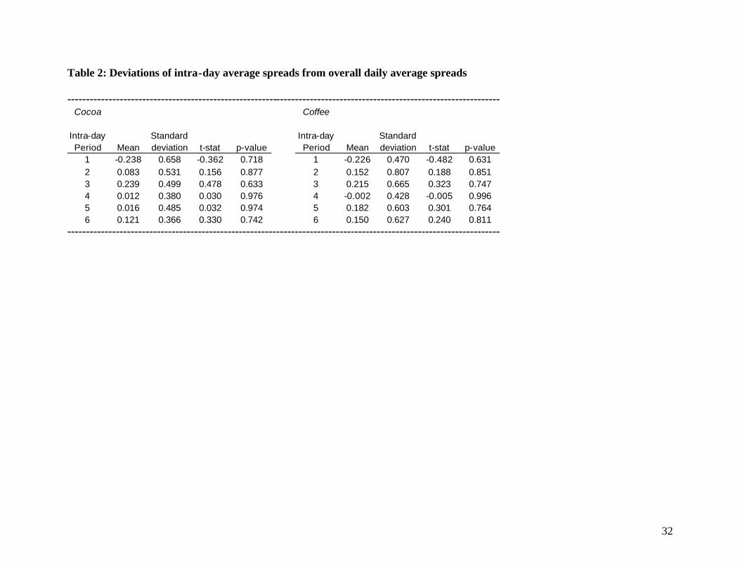
was then calculated for all days in the sample. The null hypothesis that the mean deviation for an

intra-day period was significantly different form zero was tested, and results of these tests are

reported in Table 2. We find that on average, the first period average spread is above the daily

average (as reflected by the negative deviations reported in Table 2), and generally the subsequent

periods’ average spreads are below the daily average. This suggests a weak “reverse-J” pattern of

spreads similar to that found in ap Gwilym and Thomas (2001). However, none of the intra-day

spread deviations were found to be significantly different from zero, implying that there is no

consistent pattern of significant intra-day deviation of commodity futures spreads away from the

daily average spreads over the sample period. We can thus feel comfortable in following the

significant body of research that has employed estimates of the daily average spread, and do not

apply the estimators to shorter time frames.6

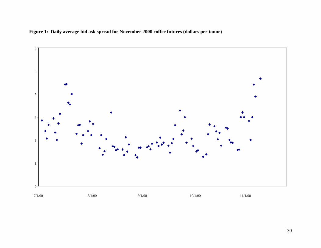
The daily spread averages for a contract in our data sample generally follow a “U-shaped”

pattern in which they are higher when the delivery date is distant, decrease as time passes, and

eventually increase as the delivery date approaches. As an example, spreads for the November

2000 coffee contract are plotted over time in Figure 1.

The transaction observations provided by LIFFE include consecutive transactions at equal

prices. From this data, a “raw” series of price changes is constructed, which is then used in the

calculation of RM. It should be noted that this type of transaction price series is not reported by the

major U.S. exchanges, and so the RM estimator could not be applied to U.S. data in the way that it

is applied here. A series consisting of strictly non-zero price changes is constructed, which is then

14

used to calculate CDP, TWM, and SW. This second price change series is thus like that which

would be reported by a U.S. futures exchange. Lastly, a series of only opposite-direction price

changes is assembled for use in calculating CFTC. This last price change series typically contains

about half as many price changes as the strictly non-zero price change series, which in turn usually

contains about half as many price changes as the completely unrestricted price change series.

Evaluation of Spread Estimator Performance

The daily average bid-ask spread is estimated for each day of each delivery over the time

period from 3 July 2000 through 24 November 2000. The serial covariance-type estimates, RM and

CDP, frequently cannot be calculated however due to price changes that exhibit positive serial

covariance. This occurs relatively more often for cocoa (about 44% of observations) than for coffee

(about 20% of observations). Within each commodity the problem occurs more often for CDP, the

serial covariance estimator using only price-changing observations. Other researchers have noted

this problem with serial covariance estimators and have offered various explanations. For instance,

Chu, Ding, and Pyun suggested that positive serial covariance in price changes could be due to

sequential information arrival. Roll suggested that market inefficiencies over short time frames

could be to blame. Observations where RM and CDP encounter the problems described above are

omitted from the analysis.

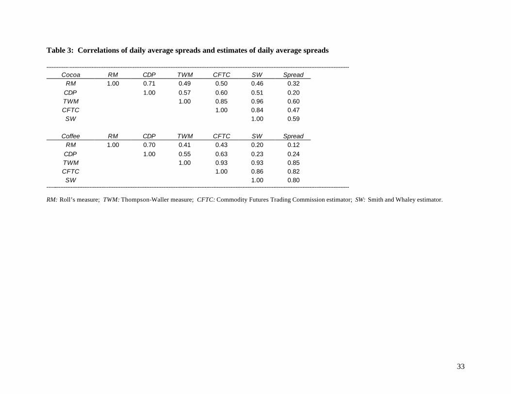
Correlations between observed and estimated daily average spreads for each market are

given in Table 3. All of the estimates are more highly correlated with the observed spreads for

coffee than for cocoa, with the exception of RM. The correlations between the serial covariance

estimates and the observed average spreads are positive, but not especially high, ranging between

0.12 and 0.32. Correlations between the remaining estimates and average spreads are more

impressive, falling in the 0.47 to 0.85 range. In this respect, TWM, SW, and CFTC appear to do a

15

much better job than RM and CDP. TWM, SW, and CFTC are highly correlated with one another,

as are RM and CDP. Thus estimators of the same type (serial covariance-type estimators or

absolute price change-type estimators) seem to be highly correlated with one another, and

noticeably less correlated with estimators of the other type. Interestingly, even though SW is

designed to estimate effective spreads, it is more highly correlated with the nominal spread

estimators (TWM and CFTC) than with the other effective spread estimators (RM and CDP).

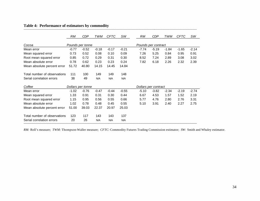
Performance of the estimators using va rious measures for all observations are given for each

commodity individually in Table 4. The performance of the estimators relative to one another is

similar within each commodity. The absolute price change-type estimators seem to perform much

better than the serial covariance type estimators by each of the performance measures. Among the

absolute price change estimators, relative performance is very similar for cocoa. However SW

performs somewhat worse than TWM and CFTC when estimating coffee spreads. Thus the relative

performance SW estimator may be somewhat inconsistent across commodities.

Comparing the absolute performance of the estimators across commodities using the mean

absolute percent error measure, the absolute price change estimators seem to perform somewhat

worse when estimating coffee spreads than when estimating cocoa spreads. We also note that all

mean errors are negative for all estimators for both commodities, suggesting that the estimators

produce downwardly biased estimates of nominal spreads in commodity futures markets. This is

consistent with the findings of ap Gwilym and Thomas for financial futures.

The results from the estimation of equation (7) for each combination of commodities are

presented in Table 5. In almost all cases, the null hypotheses that β0 = 0 is rejected at the 5% level

of significance, meaning that for the most part the differences in the biases (mean errors) reported in

Table 4 are significant. The sole exception is that the difference in the biases of TWM and CFTC

16

for cocoa is not significantly different. In most cases the null hypothesis β1 = 0 also cannot be

rejected, with the interesting exceptions being that the error variances of TWM and SW are not

significantly different for cocoa, and the error variances of CFTC and TWM are not significantly

different for coffee.

It should be noted at this point that all results reported thus far are based on all data for all

contracts. The u-shaped pattern in Figure 1 suggests that conditions over the life of a contract vary,

and thus performance of spread estimators may thus vary by time to delivery. However, only the

aggregate results are only presented as separating the data into nearby and distant groups revealed

only a single interesting difference in performance. This difference is that for cocoa, the bias of the

CFTC estimator improved to be significantly better than the TWM estimator, and the variance of the

CFTC estimator improved to be not significantly different from the SW and TWM estimators. Thus

the performance of the CFTC estimator may be somewhat better when estimating spreads for a

contract nearby delivery.

Analyzing the signs of the coefficient estimates in Table 5, the serial covariance estimators

have larger biases than the absolute price change estimators (significantly positive 0β estimates),

but lower error variances (significantly negative 1β estimates). This naturally leads one to question

which class of estimators generally has lower means of squared errors. As discussed earlier, in

some cases an F-test can be used to test the null hypothesis that both 0β and 1β from equation (7)

are zero for a pair of estimators, implying that the mean squared errors of the two estimators are not

significantly different. However if one of the two coefficient estimates is significantly negative,

this null hypothesis automatically cannot be rejected. This is the case for most of the possible pairs

of estimators in this study, and thus the Ashley methodology is largely powerless for finding

differences in the mean squared errors here. Although the statistical methodology available cannot

17

prove that the means of the squared errors of the serial covariance estimators are greater than those

of the absolute price change estimators, the relative magnitudes reported in Table 4 strongly suggest

that this is the case. Still, these results suggest that those interested in minimizing error variance (at

the expense of significantly higher error bias) may wish to consider using the serial covariance

estimators.

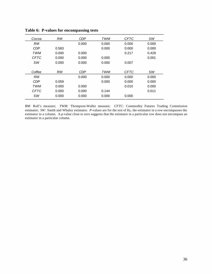
The other methodology we employ to evaluate the estimator performance is the forecast

encompassing testing procedure described previously. Probability values for the test that λ = 0

(from equation (11)) for each permutation of two estimators are presented in Table 6. In most

cases, the null hypothesis that one estimator encompasses another is rejected. In only one case is

this hypothesis not rejected across both commodities: we cannot reject that CDP encompasses RM.

Since encompassing is generally rejected, it is quite possible that a composite estimator could

provide superior estimates of nominal bid-ask spreads. In particular, one might speculate that

combining a serial covariance estimator and an absolute price change estimator might prove fruitful,

as the former will have a lower error variance, while the latter will be less biased.

III. Spreads in Electronic and Open Outcry Commodity Futures Markets

It seems therefore that spread estimators may be useful for traders not able to consistently

observe bidding and asking prices, as on U.S. exchanges. Indeed, as mentioned previously, spread

estimators may shed some light on likely transaction costs. However, of late many trading

environments have moved toward automated trading, suggesting that the costs of trading may

indeed alter. Whether or not moving to an electronic platform affects bid-ask spreads in commodity

futures markets is a question to which we now turn.

Arguments on the relative merits of open outcry and automated trading systems have

focused on two issues. First, researchers have noted that a market maker faces an adverse selection

18

problem (Copeland & Galai (1983), Glosten & Milgrom (1985)). Specifically, if a market maker

must make a commitment to buying and selling prices that will be available to all traders, she

exposes herself to counterparties with superior information. Features of the open-outrcry system

mitigate the severity of the adverse selection problem to some extent, however. In the open-outcry

environment, traders are face-to-face with their conterparties, and can thus infer from their identity

and disposition the likely nature of the information that they possess. Furthermore, if they perceive

that private information might be entering the market, traders can very rapidly adjust their offers to

buy and/or sell. In an anonymous limit order book system, however, the market maker is deprived

of these advantages. As noted by Copeland & Galai (1983), a limit order can be likened to a short

option position with a time to maturity equal to the time required to withdraw the order. In an

anonymous limit order book system the market maker is forced to make this option available to all

traders, and will not be able to quickly discern when the well- informed are entering the market.

Market makers will thus require compensation, in the form of wider bid-ask spreads, for this

increased risk that they will be at an informational disadvantage on any given trade. It is thus

widely believed that a more pronounced adverse selection problem will tend to increase transaction

costs in anonymous electronic trading, relative to open outcry trading.

The adverse selection problem may be more acute in some markets than in others, however.

The model of Subrahmanyan (1991) suggests that the information costs paid in a market for a

basket of assets (e.g. a stock index futures market) are lower than those paid in a market for an

individual asset. Also, the values of some assets are determined largely by information that is

naturally public in nature. For example, the values of debt instruments are likely to be a function

primarily of the state of the macroeconomy, which is relatively easily observed in countries that

report a comprehensive set of national accounts. Prices in other markets, however, are likely to be

19

determined by information that is held by a relatively small number of agents (e.g. an agricultural

commodity market). In these types of markets, Foster & Viswanathan (1994) suggest that the well-

informed traders will indeed capitalize on their advantageous position. Thus the impact on

transaction costs of moving from open outcry to automated trading is likely to depend on the

specific nature of the market, and the results found in financial markets may not apply to

commodity futures markets.

The order processing component of transaction costs are the other issue on which the

relative merits of open outcry and automated systems have been compared. It has been suggested

that automated trading should offer significant operational efficiencies relative to open outcry

trading, thereby potentially reducing transaction costs (Massimb and Phelps (1994), Pirrong

(1996)). Specifically, fewer people need be employed in an electronic system, and electronic

trading should result in fewer costly mistakes (out-trades) than open-outcry trading. A significant

fixed cost is likely to be associated with automating trading, however, and there may be much less

potential for gains in efficiency in a fairly low volume futures market. On numerous levels

therefore we have reason to believe that results regarding the impact on spread magnitudes of

automating trading found in financial futures markets may not apply to commodity futures markets.

Despite the possible differences in impact it is worthwhile providing a very brief (and by no

means comprehensive) summary of some results found in the financial markets. However, the

summary is by no means comprehensive. Frino, McInish, and Toner (1998) (among others)

examined simultaneous electronic and open outcry trading in German Bund futures, finding wider

spreads on the automated exchange. They also found that during electronic trading, there was a

larger marginal effect of an increase in volatility on spread magnitudes. Wang (1999) analyzed the

differences between daytime open outcry and evening electronic trading in financial futures at an

20

exchange, finding results similar to Frino, McInish, and Toner. Tse and Zabotina (2001) looked at

trading in FTSE stock index futures before and after trading was automated at LIFFE, finding that

spreads were narrower after the trading was automated. Thus the evidence regarding the relative

magnitudes of bid-ask spreads in electronic and open outcry financial futures markets is mixed.

Here, we will compare the magnitudes of bid-ask spreads before and after a move from open

outcry to automated trading in the same two commodity futures markets evaluated earlier (cocoa

and coffee). Compared to the financial futures markets examined in the studies cited above, these

markets have significantly lower trading volumes.7 These lower volumes call into question the

potential for increasing operational efficiency by automating trading. Also, for reasons discussed

earlier, the impact of moving to electronic trading on the adverse selection component of transaction

costs is likely to be different for these markets than it is for the financial markets studied previously.

The relative proportions of well- informed traders are different in commodity futures markets than in

financial markets, and the information that determines prices in these markets is inherently less

public in nature. We posit the following hypotheses:

Hypothesis 1: In anonymous electronic trading, bid-ask spreads have a greater tendency to widen in

response to increases in volatility (relative to open outcry trading).

Hypothesis 2: Market makers will face a significant adverse selection problem in an anonymous

electronic commodity futures market, and net transaction costs, as measured by bid-ask spreads,

will be higher than those observed in the open outcry system.

Methodology for Comparing Electronic and Open Outcry Spreads

We will use the methodology employed by Frino, McInish, and Toner to compare spreads

on a security traded at two different exchanges while controlling for factors known to affect

spreads. Rather than comparing spreads at two different exchanges, however, we will be comparing

21

spreads before and after a switch from open-outcry to electronic trading, as in Tse and Zabotina.

The empirical model is as follows:

tettet volumeDpricevolumeDSpread 43210 )(var βββββ ++++=

ttte pricepriceD εββ +++ 65 )(var . (12)

Spreadt is the average nominal bid-ask spread during period t, De is a dummy variable that is zero

for an open-outcry observation and one for an electronic observation, volumet is the total volume of

futures traded, vart(price) is the variance of spread midpoints during period t, and pricet is the

average spread midpoint during period t. Consistent with McInish and Wood (1992) and Frino,

McInish, and Toner, square roots of the determinants of the spread are used to prevent outlying

observations from exerting undue influence on the regression results. Theory suggests that we

should expect a negative relationship between spread magnitude and volume of trade, and a positive

relationship between spread magnitudes and price variability (Copeland and Galai (1983)). These

results have also been observed in empirical studies (examples include McInish and Wood (1992)

for stocks, and Ding (1999) for futures). The relationship between quoted spreads and the level of

the price of the commodity is expected to be positive for two reasons. First, the volatility of prices

of commodities tends to increase as the prices themselves increase. Thus it is possible that the price

coefficient in the model might “pick up” some of the positive effect of price variance on spreads. A

similar argument was used by Stoll (1978).8 Second, and perhaps more importantly, it is expected

that percentage spreads should be somewhat steady. In the words of Demsetz (1968), a positive

relationship is expected between nominal spreads and the price level so as to “equalize the cost of

transacting per dollar exchanged.”

22

Data used in Comparing Electronic and Open Outcry Spreads

Nominal spread observations must be constructed differently when using the electronic

trading record rather than the open outcry trading record, taking into consideration the different

trading mechanisms. In the electronic system at LIFFE, bid and ask price observations are the

result of standing limit orders, and need not be acted upon immediately as in open-outcry trading.

This essentially means that there is now a spread observation at every point in time during the

trading day. For each trading day from 27 November 2000 through 11 May 2001, a time series of

observations of the prevailing spread for each second was constructed for the nearby futures. A

daily average spread was then calculated by averaging over the observations for each second.

Before controlling for the determinants of spreads, we find similar average daily spreads for

nearby coffee futures in the electronic and open-outcry periods, at $1.97 and $2.07 per tonne,

respectively. We observe a noticeable increase in daily average spreads for cocoa, however. Over

the open-outcry period, the average spread for nearby futures is £1.56 per tonne. In the electronic

period, the average spread is a noticeably higher £3.31 per tonne, and there is a much greater

variability relative to the open-outcry period. Cocoa prices experienced a significant increase

(which is usually accompanied by an increase in volatility) shortly after the move to automated

trading, however, and it is therefore important to control for such factors before drawing any

conclusions.

Results of Comparing Electronic and Open Outcry Spreads

The model in equation (12) was estimated for each of the two commodity futures markets,

and robust standard errors for the parameter estimates were estimated using the Newey and West

(1987) procedure. Results are presented in Table 7. For cocoa, we find that the volume and

volatility coefficients not significant. This is somewhat surprising, although these results may be

23

due to the fact that there was little variation in these variables (and indeed the dependent variable

itself) during the open-outcry period. While not significant, the coefficient on the price standard

deviation term has the expected sign. The price level term has a positive coefficient, as expected,

and is highly significant. Also, we find a significantly negative constant term. Although this may

seem counter- intuitive given that the dependent variable is always positive, the results must be

taken as a whole. The square root the price variable has a mean of 26.3, with a standard deviation

of 2.1. Thus the highly significant coefficient on this variable of 0.329 implies that this term is

consistently adding about £8 to the predicted spread. This suggests that the negative constant is no

cause for concern.

The coefficient on the electronic dummy variable is positive and significant at the 10%

level. We therefore find that, after controlling for other explanatory factors, the switch to electronic

trading has widened observed spreads in the cocoa futures market by about £0.64 per tonne. The

coefficient for the volume interaction term is negative and significant. This indicates that cocoa

spreads have become sensitive to volume since the move to electronic trading. Increases in the

volume of trade cause decreases in the spread, whereas no such effect was observed during the

open-outcry period. We also find a significantly positive volatility interaction term, suggesting that

cocoa spreads have also become sensitive to volatility following the move to automated trading.

Turning to the coffee results, we find coefficients of the expected signs for the volume and

volatility terms, with the volatility term being significant. As in the cocoa model, the coefficient on

the price level is positive and significant. Also as in the cocoa regression, we find a positive and

significant electronic dummy term, a positive and significant volatility interaction term, but no

significant volume interaction term. Thus, as in the cocoa market, we find tha t spreads in the coffee

24

market have become more sensitive to the level of price variability than they were during open

outcry trading, and have generally widened after controlling for spread determinants.

In both markets we find the result that transaction costs, as measured by the magnitudes of

bid-ask spreads, have a greater tendency to increase as prices become more volatile, supporting our

Hypothesis 1. This is observation is consistent with the suggestion that market makers in the

anonymous automated market cannot distinguish between noise trading and information trading.

They thus have an increased tendency to widen spreads during high-volatility periods as

compensation for the risk that they may be at an informational disadvantage. This result is

consistent with results from financial futures research (Frino, McInish, and Toner (1998) and Wang

(1999)).

The finding that spreads have widened in the cocoa and coffee futures markets suggests that

the net effect of automating trading has been to increase transaction costs. We thus find support for

Hypothesis 2. Specifically, these results suggest that lower order processing costs are outweighed

by increases in transaction costs due to a more severe adverse selection problem. This suggests that

one of the expected benefits of electronic trading, reduced transaction costs as manifested by

narrower bid-ask spreads, may not materialize, depending on the nature of the market in question.

Commodity futures markets in particular, with their lower volumes and higher proportions of

information traders, may not realize lower transaction costs by automating trading.

Given that we have found that the size of the spread has changed with the change in

environment a critical question is that of the economic significance of the differences in spreads

observed since the move to electronic trading. Indeed, from both a market participant and exchange

point of view having an understanding of the monetary implications of executing a trade in the

electronic environment is paramount. Therefore, similar to an analysis carried out in Venkataraman

25

(2001), we use our empirical models of coffee and cocoa spreads to calculate the potential increases

in transaction costs that have been realized since trading was automated. Specifically, we calculate

the estimated impact on the spread due to the automation of trading at time t as

)(varˆˆˆ541 pricevolumeChange ttt βββ ++= (13)

for each commodity, where the coefficient are from the appropriate estimate of equation (12). Note

that this represents the estimated average change in the spread per ton on a particular day. We then

multiply this number by the number of tons in the contract to arrive at an estimated change in the

spread per contract. This value is then averaged over the entire electronic trading period in our

sample, weighting each day’s observation using that day’s volume. We calculate these values as

£6.46 for cocoa and $3.94 for coffee. These numbers might be interpreted roughly as the average

increase (due the automation of trading) in transaction cost per contract that is being realized by a

trader who completes a round-turn using market orders to both enter and exit the position. Care

must be exercised in this interpretation, however, as these are nominal spreads rather than effective

spreads.9 Nonetheless, these numbers give some sense of the economic impact of the move to

automated trading in these commodity futures markets and illustrate that for the commodity markets

studied here, the change in environment has increased transaction costs.

IV. Conclusions

This study has investigated issues regarding nominal bid-ask spreads in relatively low-

volume commodity futures markets. Several spread estimators were applied using open outcry

transaction data from the LIFFE coffee and cocoa markets, and the resulting estimates were

compared to observed nominal bid-ask spreads. The mean absolute price change estimators, TWM,

CFTC, and SW, perform better at estimating daily average nominal spreads than the serial

covariance estimators, RM and CDP, by the bias and mean square error criteria. The serial

26

covariance estimators have lower error variances, however. Encompassing test results generally

confirm that the estimators do not encompass one another, and there may be gains from combining

estimates. These results should be of interest to those who wish to estimate potential transaction

costs in open outcry futures markets that report transaction price data, but not bid and ask data.

We find an increased tendency for spreads to widen as volatility increases, which is

consistent with the argument that market makers face a worse adverse selection problem in

anonymous electronic trading. Also, we find that net transaction costs, as measured by bid-ask

spreads, have widened in the commodity futures markets studied here, even after controlling for

spread determinants. This suggests that lower order processing costs in automated trading may be

outweighed by increases in transaction costs due to a more severe adverse selection problem. It

thus seems that some of the benefits that have been realized by automating trading in some financial

futures markets may not be realized in commodity futures markets, which tend to have lower

volumes and are inherently different in nature.

27

Bibliography ap Gwilym, O. and Thomas, S. (2001): An Empirical Investigation of Quoted and Implied Bid-Ask Spreads on Futures Contracts. Journal of International Financial Markets, Institutions, and Money, forthcoming. Ashley, R., Granger, C. W. J., & Schmalensee, R. (1980): Advertising and Aggregate Consumption: An Analysis of Causality. Econometrica, 48, 1149-1167. Bae, K., Chan, K., & Cheung, Y. (1998): The Profitability of Index Futures Arbitrage: Evidence From Bid-Ask Quotes. Journal of Futures Markets, 18, 743-763. Bhattacharya (1983): Transactions Data Tests of Efficiency of the Chicago Board of Options Exchange. Journal of Financial Economics, 12, 161-186. Chu, Q. C., Ding, D. K., & Pyun, C. S. (1996): Bid –Ask and Spreads in the Foreign Exchange Market. Review of Quantitative Finance and Accounting, 6, 19-37. Copeland, Thomas E. & Galai, Dan (1983): Information Effects on the Bid-Ask Spread. Journal of Finance, 38, 1457-1469. Demsetz, H. (1968): The Cost of Transacting. Quarterly Journal of Economics, 82:33-53. Ding, David K. (1999): The Determinants of Bid-Ask Spreads in the Foreign Exchange Futures Markets: A Microstructure Analysis. Journal of Futures Markets, 19, 307-324. Foster, F. Douglas & Viswanathan, S. (1994): Strategic Trading with Asymmetrically Informed Traders and Long-Lived Information. Journal of Financial and Quantitative Analysis, 29, 499-518. Frino, A., McInish, T. H., & Toner, M. (1998): The Liquidity of Automated Exchanges: New Evidence from German Bund Futures. Journal of Internationa l Financial Markets, Institutions, and Money, 8, 225-241. Glosten, Lawrence R. & Milgrom, Paul R. (1985): Bid , Ask, and Transaction Prices in a Specialist Market with Heterogeneously Informed Traders. Journal of Financial Economics, 14, 71-100. Granger, C. W. J. & Newbold, P. (1973): Some Comments on the Evaluation of Economic Forecasts. Applied Economics, 5, 35-47. Harvey, D. I., Leybourne, S. J., & Newbold, P. (1998): Test for Forecast Encompassing. Journal of Business & Economic Statistics, 16, 254-259. Laux, P.A. and A.J. Senchack. (1992). Bid-Ask Spreads in Financial Futures. Journal of Futures Markets, 12 (6) 621 – 634.

28

Lee, C. & Ready, M. (1991): Inferring Trade Direction From Intraday Data. Journal of Finance, 46, 733-746. Locke P. R., & Venkatesh, P. C. (1997): Futures Market Transaction Costs. Journal of Futures Markets, 17, 229-245. Ma, C. K., Peterson, R. L., & Sears, R. S. (1992): Trading Noise, Adverse Selection, and Intraday Bid-Ask Spreads in Futures Markets. The Journal of Futures Markets, 12, 519-538. Massimb, Marcel N., & Phelps, Bruce D. (1994): Electronic Trading, Market Structure and Liquidity. Financial Analysts Journal, 50, 39-50. McInish, T., & Wood, R. (1992): An Analysis of Intraday Patterns in Bid/Ask Spreads for NYSE Stocks. Journal of Finance, 47, 753-763. Newey, W., & West, K. (1987): A Simple Positive Semi-definite, Heteroskedasticity and Autocorrelation Consistent Covariance Matrix. Econometrica, 51, 76-89. Petersen, M. A. & Fialkowski, D. (1994): Posted Versus Effective Spreads: Good Prices or Bad Quotes? Journal of Financial Economics, 35, 269-292. Pirrong, Craig (1996): Market Liquidity and Depth on Computerized and Open Outcry Systems: A Comparison of DTB and LIFFE Bund Contracts. The Journal of Futures Markets, 5, 519-543. Roll, R. (1984): A Simple Implicit Measure of the Effective Bid-Ask Spread in an Efficient Market. Journal of Finance, 23, 1127-1139. Shyy, G., Vijayraghavan, V., & Scott-Quinn, B. (1996): A Further Investigation of the Lead-Lag Relationship Between the Cash Market and Stock Index Futures Market With the Use of Bid-Ask Quotes: The Case of France. Journal of Futures Markets, 16, 405-420. Silber, W. (1984): Marketmaker Behavior in an Auction Market: An Analysis of Scalpers in Futures Markets. Journal of Finance, 4, 937-953. Smith, T., & Whaley, R. E. (1994): Estimating the Effective Bid/Ask Spread from Time and Sales Data. Journal of Futures Markets, 14, 437-456. Stoll, H. (1978): The Pricing of Security Dealer Services: An Empirical Study of NASDAQ Stocks. Journal of Finance, 33, 1153-1172. Subrahmanyam, Avanidhar (1991): A Theory of Trading in Stock Index Futures. Review of Financial Studies, 4, 17-51. Thompson, S., Eales, J. S., & Siebold, D. (1993): Comparison of Liquidity Costs Between the Kansas City and Chicago Wheat Futures Contracts. Journal of Agriculture and Resource Economic, 18, 185-197.

29

Thompson, S. R., & Waller, M. (1988): Determinants of Liquidity Costs in Commodity Futures Markets. Review of Futures Markets, 7, 110-126. Tse, Y. (1999): Market Microstructure of FT-SE 100 Index Futures: An Intraday Empirical Analysis, The Journal of Futures Markets, 19, 31 – 58. Tse, Y. & Zabotina, T. V. (2001): Transaction Costs and Market Quality: Open Outcry Versus Electronic Trading, The Journal of Futures Markets, 21, 713-735. Venkataraman, K. (2001): Automated Versus Floor Trading: An Analysis of Execution Costs on the Paris and New York Exchanges. Journal of Finance, 56, 1445-1485. Wang, H. K. W., Yau, J., & Baptiste, T. (1997): Trading Volume and Transaction Costs in Futures Markets. Journal of Futures Markets, 17, 757-780. Wang, J. (1999): Asymmetric Information and the Bid-Ask Spread: An Empirical Comparison Between Automated Order Execution and Open Outcry Auction. Journal of International Financial Markets, Institutions, and Money, 9, 115-128. White, H. (1980): A Heteroscedasticity-Consistent Covariance Matrix Estimator and a Direct Test for Heteroscedastcity. Econometrica, 48, 817 – 838.

30

Figure 1: Daily average bid-ask spread for November 2000 coffee futures (dollars per tonne)

0

1

2

3

4

5

6

7/1/00 8/1/00 9/1/00 10/1/00 11/1/00

31

Table 1: Example of LIFFE coffee futures data --------------------------------------------------------------------------------------------------------------------------------------------------------------------------------

Date Time Delivery Type Volume Price 10/27/00 10:03:50 Nov-00 Bid 0 701 10/27/00 10:04:12 Nov-00 Bid 0 702 10/27/00 10:04:49 Nov-00 Ask 0 702 10/27/00 10:04:50 Nov-00 Bid 0 701 10/27/00 10:04:51 Nov-00 Trd 3 702 10/27/00 10:05:16 Nov-00 Ask 0 703 10/27/00 10:05:31 Nov-00 Trd 5 701 10/27/00 10:05:45 Nov-00 Trd 5 701 10/27/00 10:07:09 Nov-00 Trd 20 703 10/27/00 10:08:18 Nov-00 Bid 0 702 10/27/00 10:11:12 Nov-00 Trd 20 702 10/27/00 10:11:24 Nov-00 Trd 1 703 10/27/00 10:18:15 Nov-00 Ask 0 702 10/27/00 10:18:16 Nov-00 Bid 0 701 10/27/00 10:19:37 Nov-00 Trd 1 702 10/27/00 10:19:38 Nov-00 Trd 1 702 10/27/00 10:19:41 Nov-00 Trd 1 701

-------------------------------------------------------------------------------------------------------------------------------------------------------------------------------- Source: London International Financial Futures and Options Exchange (LIFFE). “Type” refers to type of price observation. “Trd” denotes a trade observation.

32

Table 2: Deviations of intra-day average spreads from overall daily average spreads --------------------------------------------------------------------------------------------------------------------

Cocoa Coffee

Intra-day Standard Intra-day Standard Period Mean deviation t-stat p-value Period Mean deviation t-stat p-value

1 -0.238 0.658 -0.362 0.718 1 -0.226 0.470 -0.482 0.631 2 0.083 0.531 0.156 0.877 2 0.152 0.807 0.188 0.851 3 0.239 0.499 0.478 0.633 3 0.215 0.665 0.323 0.747 4 0.012 0.380 0.030 0.976 4 -0.002 0.428 -0.005 0.996 5 0.016 0.485 0.032 0.974 5 0.182 0.603 0.301 0.764 6 0.121 0.366 0.330 0.742 6 0.150 0.627 0.240 0.811

--------------------------------------------------------------------------------------------------------------------

33

Table 3: Correlations of daily average spreads and estimates of daily average spreads --------------------------------------------------------------------------------------------------------------------------------------------------------------------------------

Cocoa RM CDP TWM CFTC SW Spread RM 1.00 0.71 0.49 0.50 0.46 0.32

CDP 1.00 0.57 0.60 0.51 0.20 TWM 1.00 0.85 0.96 0.60 CFTC 1.00 0.84 0.47 SW 1.00 0.59

Coffee RM CDP TWM CFTC SW Spread

RM 1.00 0.70 0.41 0.43 0.20 0.12 CDP 1.00 0.55 0.63 0.23 0.24 TWM 1.00 0.93 0.93 0.85 CFTC 1.00 0.86 0.82 SW 1.00 0.80

-------------------------------------------------------------------------------------------------------------------------------------------------------------------------------- RM: Roll’s measure; TWM: Thompson-Waller measure; CFTC: Commodity Futures Trading Commission estimator; SW: Smith and Whaley estimator.

34

Table 4: Performance of estimators by commodity ------------------------------------------------------------------------------------------------------------------------------------------------------------------------------------------------------

RM CDP TWM CFTC SW RM CDP TWM CFTC SW Cocoa Pounds per tonne Pounds per contract Mean error -0.77 -0.52 -0.18 -0.17 -0.21 -7.74 -5.19 -1.84 -1.65 -2.14 Mean squared error 0.73 0.52 0.08 0.10 0.09 7.26 5.25 0.84 0.95 0.91 Root mean squared error 0.85 0.72 0.29 0.31 0.30 8.52 7.24 2.89 3.08 3.02 Mean absolute error 0.78 0.62 0.23 0.23 0.24 7.82 6.18 2.26 2.32 2.39 Mean absolute percent error 51.72 40.80 14.15 14.45 14.84 Total number of observations 111 100 149 149 148 Serial correlation errors 38 49 N/A N/A N/A Coffee Dollars per tonne Dollars per contract Mean error -1.02 -0.76 -0.47 -0.44 -0.55 -5.10 -3.82 -2.34 -2.19 -2.74 Mean squared error 1.33 0.91 0.31 0.30 0.44 6.67 4.53 1.57 1.52 2.19 Root mean squared error 1.15 0.95 0.56 0.55 0.66 5.77 4.76 2.80 2.76 3.31 Mean absolute error 1.02 0.78 0.48 0.45 0.55 5.10 3.91 2.40 2.27 2.75 Mean absolute percent error 51.00 39.03 22.37 20.97 25.03 Total number of observations 123 117 143 143 137 Serial correlation errors 20 26 N/A N/A N/A ------------------------------------------------------------------------------------------------------------------------------------------------------------------------------------------------------ RM: Roll’s measure; TWM: Thompson-Waller measure; CFTC: Commodity Futures Trading Commission estimator; SW: Smith and Whaley estimator.

35

Table 5: Coefficient estimates and p-value for differences in bias and variance components for each pair of bid-ask spread estimators ----------------------------------------------------------------------------------------------------------------------------------------------------------------------------------------------------------

β0 β1

Cocoa CDP TWM CFTC SW CDP TWM CFTC SW RM 0.230 0.586 0.624 0.563 0.205 -0.319 -0.219 -0.358

(0.000) (0.000) (0.000) (0.000) (0.000) (0.000) (0.000) (0.000)

CDP 0.324 0.378 0.300 -0.475 -0.397 -0.509

(0.000) (0.000) (0.000) (0.000) (0.000) (0.000)

TWM 0.019 -0.032 0.084 -0.020

(0.084) (0.000) (0.001) (0.137)

CFTC -0.052 -0.103

(0.000) (0.000)

Coffee CDP TWM CFTC SW CDP TWM CFTC SW

RM 0.219 0.566 0.615 0.522 0.077 -0.340 -0.301 -0.275

(0.000) (0.000) (0.000) (0.000) (0.022) (0.000) (0.000) (0.000)

CDP 0.316 0.369 0.290 -0.385 -0.329 -0.338

(0.000) (0.000) (0.000) (0.000) (0.000) (0.000)

TWM 0.031 -0.079 0.048 0.106

(0.043) (0.000) (0.054) (0.000)

CFTC -0.096 0.076

(0.000) (0.014) ----------------------------------------------------------------------------------------------------------------------------------------------------------------------------------------------------------

RM: Roll’s measure; TWM: Thompson-Waller measure; CFTC: Commodity Futures Trading Commission estimator; SW: Smith and Whaley estimator. β0 > 0 implies that the bias of the estimator in the row is greater than the bias of the estimator in the column. β0 < 0 implies the opposite. β1 > 0 implies that the variance of the estimator in the row is greater than the variance of the estimator in the column. β1 < 0 implies the opposite. P – values close to zero suggest that the bias and or/variance of two estimators is statistically different

36

Table 6: P-values for encompassing tests ------------------------------------------------------------------------------------------------------------------------------------------------------

Cocoa RM CDP TWM CFTC SW RM 0.000 0.000 0.000 0.000 CDP 0.583 0.000 0.000 0.000 TWM 0.000 0.000 0.217 0.429 CFTC 0.000 0.000 0.000 0.001 SW 0.000 0.000 0.000 0.007

Coffee RM CDP TWM CFTC SW

RM 0.000 0.000 0.000 0.000 CDP 0.059 0.000 0.000 0.000 TWM 0.000 0.000 0.010 0.000 CFTC 0.000 0.000 0.144 0.011 SW 0.000 0.000 0.000 0.000

------------------------------------------------------------------------------------------------------------------------------------------------------ RM: Roll’s measure; TWM: Thompson-Waller measure; CFTC: Commodity Futures Trading Commission estimator; SW: Smith and Whaley estimator. P-values are for the test of H0: the estimator in a row encompasses the estimator in a column. A p-value close to zero suggests that the estimator in a particular row does not encompass an estimator in a particular column.

37

Table 7: Determinants of Daily Average Spreads Regression Results ---------------------------------------------------------------------------------------------------

Cocoa Coffee Coefficient Coefficient estimate p-value estimate p-value

Constant -6.726 0.000 -2.105 0.050 De 0.637 0.090 0.678 0.020

Sqr(volume) 0.000 0.865 -0.006 0.109 Sqr(variance) 0.071 0.450 0.068 0.002

DeSqr(volume) -0.018 0.015 -0.003 0.719 DeSqr(variance) 0.469 0.036 0.083 0.078

Sqr(price) 0.329 0.000 0.142 0.000

R2 0.715 0.336 --------------------------------------------------------------------------------------------------- De is a dummy variable that is zero for an open-outcry observation and one for an electronic observation, volume is the total volume of futures traded, variance is the variance of spread midpoints, and price is the average spread midpoint for a day.

38

Endnotes 1 Research into spreads can be classified as concerning nominal, effective, or quoted spreads. In this paper, we define quoted spreads as those determined by the bids and offers that officially designated market makers are required to simultaneously quote in a specialist system, such as that of the New York Stock Exchange. In futures markets, there are no officially designated monopolistic market makers, and hence no quoted spreads. Instead, there are simply prevailing best bidding and asking prices (which may be provided by different traders) that together imply a nominal spread. Here we define effective spreads to be the average transfer of wealth from market participants to liquidity providers. These differ from quoted spreads due to trading inside the quoted prices in a specialist system (Roll 1984; Petersen and Fiakowski, 1994). In futures markets, effective spreads differ from nominal spreads due to liquidity providers exiting positions at zero profit (“scratch sales”) and also due to trading directly between non- liquidity traders (Smith and Whaley, 1994; Locke and Venkatesh, 1997). 2 Another estimator, proposed by Bhattacharya (1983), is the average of an even smaller subset of absolute price changes. Because the markets considered here have fairly low volumes except in the contracts nearest delivery, this estimator would have frequently not produced an estimate. Those interested in estimating nominal spreads for higher volume commodities or contracts may wish to consider this estimator. 3 All data are subjected to a screening algorithm and obviously erroneous observations are removed. 4 This stands in contrast to electronic data whereby any bids or asks that are reported by the exchange are standing limit orders and will exist until the trader actively withdraws the bid or ask. As such, the bid-ask data series from an electronic trading environment looks very different than that from an open outcry environment. 5 Prices must be successive. For example, suppose a bid occurs at 10:00:00, and another, different bid occurs at 10:00:03. Then, an ask is observed at 10:00:07. This ask would not be mated with the first bid, even though they both occurred within 10 seconds of one another. In an earlier version of the paper the same analysis was conducted on the open outcry trade data provided by LIFFE from 1996 to July 2000 (before the reporting system changed). As mentioned previously, this data series meant that many of the bids and asks reported within the same minute did not represent a valid spread (e.g., non positive spreads) and so did not represent the true course of events within that minute. Results from this analysis, that excluded these non-positive spreads were not entirely dissimilar to the results presented in this paper and are excluded to conserve space. They are, however, available from the authors upon request. 6 Indeed, spread estimators have been used to estimate spreads over even longer time periods. For instance, Laux and Senchack (1992) estimated monthly average spreads in financial futures markets and used these estimates to carry out their analysis.

39

7 For example, between July 2000 and June 2001, volume on the FTSE 100 futures contract at LIFFE was 9,033,641, whereas volumes on the cocoa and coffee markets were 1,408,945 and 1,271,816 respectively 8 Stoll was dealing with stocks rather than commodities. He argued that the risk associated with a stock decreased as the price of a stock increased, and therefore he expected to find a negative relationship between spreads and the price level of the underlying security. Here we use a similar argument, but expect to find an effect opposite to that found by Stoll due to the differences in the instruments under consideration. 9 This interpretation of the nominal spread is safe for the automated market, as a market order cannot be executed within the prevailing nominal spread. In the open outcry market, traders entering market orders may have enjoyed effective spreads that were lower than nominal spreads. This implies, however, the measures of the economic significance of the wider spreads that we calculate and interpret can be considered conservative.