The Eighth International Conference onComputational Fluid Dynamics (ICCFD8),Chengdu, Sichuan, China, July 14–18, 2014

ICCFD8-2014-0203

Benchmarking Optimization Algorithms forWing Aerodynamic Design Optimization

Zhoujie Lyu1∗, Zelu Xu1 and Joaquim R. R. A. Martins1

1 Department of Aerospace Engineering, University of Michigan, Ann Arbor, MI, USA

Abstract: Aerodynamic design optimization requires large computational resources, since eachdesign evaluation requires the solution of a system of partial differential equations in a three di-mensional domain. Thus, the choice of optimization algorithm is critical, as it directly affectsthe number of required design evaluations to reach the optimum design. To help designers makean informed choice, we benchmark several optimization algorithms, including gradient-based andgradient-free methods using three test problems of increasing difficulty: a multi-dimensional Rosen-brock function, a RANS-based aerodynamic twist optimization problem and an aerodynamic shapeoptimization problem. The majority of the gradient-based optimizers successfully solved all threetest problems, while the gradient-free methods require two to three orders of magnitude more com-putational effort when compared to the gradient-based methods. Thus, gradient-based algorithmsare the only viable option for solving large-scale aerodynamic design optimization problems.

Keywords: aerodynamic shape optimization, benchmarking, wing design, adjoint method.

1 IntroductionWith the advancement of high performance computing, numerical simulation and optimization of complexand large-scale aircraft design problems has become possible. Aerodynamic shape optimization of a transonicwing is an example of such complex design problems, often solved with respect to hundreds of design variables.Computational fluid dynamics (CFD) with a Reynolds-averaged Navier–Stokes (RANS) model is often usedin aerodynamic shape optimization to accurately capture the flow, which makes computing the objectivefunction computationally intensive. Therefore, performing high-fidelity aerodynamic shape optimizationremains a challenging and expensive task [1].

The optimization can be performed with gradient-based or gradient-free methods. Gradient-based meth-ods are best when an efficient gradient evaluation is available. The computational expense of evaluatingthe gradient using finite difference or complex step methods [2] is prohibitive for aerodynamic shape opti-mization with respect to hundreds of variables. The adjoint method, however, can provide accurate andefficient gradient evaluations [3, 4], and adjoint-based aerodynamic shape optimization has been widelyused [5, 6, 7, 8, 9]. The gradient-free methods are generally simpler to implement, and claim to find theglobal optimum, but the computational cost is higher. In this paper, we investigate the local optima in aero-dynamic shape optimization of a transonic wing. In addition, we also compare the optimization algorithmsusing this benchmark.

The aerodynamic shape optimization has been well-studied using various approaches. Sasaki et al. [10]applied an adaptive range multiobjective genetic algorithm (ARMOGA) to aerodynamic wing design. Afour-objective optimization of wing shape and planform were presented using 72 design variables, subjectto thickness and planform shape constraints. Moigne and Qin [11] studied aerodynamic shape optimizationbased on a discrete adjoint of a Reynolds-averaged Navier–Stokes (RANS) solver. A variable-fidelity opti-mization method combining low- and high-fidelity models was used. The optimization reduced 23% dragon a RAE2822 airfoil and 15% on a ONERA M6 wing. Their results showed that using a variable-fidelity

∗Corresponding author’s email: peterlyu@peterlyu.com.

1

method that performs most of the optimization on a low-fidelity, low-cost model (Euler equations on a coarsegrid) reduces the overall computing time.

Lyu et al. [8] presented the results of lift-constrained drag minimization of the AIAA Aerodynamic DesignOptimization Discussion Group (ADODG) Common Research Model wing1 using a RANS solver. A 8.5%drag reduction was achieved using a multilevel optimization approach. The same optimization was alsoperformed starting from a randomly generated initial design, and closely spaced local optima were observed.

Several authors compared the performance of different optimization methods. Foster and Dulikravich [12]compared a hybrid gradient method and a hybrid genetic algorithm for a three dimensional aerodynamiclifting body design. Zingg et al. [13] performed a comparison of genetic algorithm and gradient methodsin aerodynamics airfoil optimization. Genetic algorithm required 5–200 times more function evaluationsthan gradient-based methods with adjoint sensitivity. They suggested genetic algorithm was more suitedfor preliminary design with low-fidelity models. Gradient-based optimizers may be more appropriate fordetailed designs with high-fidelity models. Obayashi and Tsukahara [14] compared a gradient-based methodwith simulated annealing, and a genetic algorithm on an airfoil lift maximization problem. The geneticalgorithm required the highest number of function evaluation. However, the genetic algorithm achieved thebest design compared to the other two methods. Frank and Shubin [15] compared one-dimensional duct flowoptimization with finite-difference gradients, optimization with analytic gradients, and an all-at once methodwhere the flow and design variables are simultaneously altered. They concluded that the optimization withanalytic gradients was the best approach that can be retrofitted to most existing codes.

In this paper, we extend the previous studies of optimizer comparison and local optima using high-fidelity aerodynamic shape optimization. We compare several optimization algorithms including 6 gradient-based methods—SNOPT, PSQP, SLSQP, IPOPT, CONMIN, GCMMA—and 2 gradient-free methods—ALPSO, NSGA2. We test those optimizers using a multi-dimensional Rosenbrock function, a wing twistoptimization problem, and a wing shape optimization problem. The strengths and weaknesses of eachmethod are discussed. This paper is organized as follows. In Section 2, we discuss the computational toolsused in this study. The results of multi-dimension Rosenbrock function are presented in Section 3. Theaerodynamic twist optimization is shown in Section 4, and finally, the aerodynamic shape optimization isdiscussed in Section 5, followed by the conclusions.

2 MethodologyThis section describes the numerical tools and methods that we used for the aerodynamic shape optimizationstudies. These tools are components of the framework for multidisciplinary design optimization (MDO) ofaircraft configurations with high fidelity (MACH) [16]. MACH can perform the simultaneous optimizationof aerodynamic shape and structural sizing variables considering aeroelastic deflections [17]. However, inthis paper we use only the components of MACH that are relevant for aerodynamic shape optimization: thegeometric parametrization, mesh perturbation, CFD solver, and optimization algorithm.

2.1 Geometric ParametrizationWe use a free-form deformation (FFD) volume approach to parametrize the wing geometry [18]. The FFDvolume parametrizes the geometry changes rather than the geometry itself, resulting in a more efficient andcompact set of geometry design variables, thus making it easier to manipulate complex geometries. Anygeometry may be embedded inside the volume by performing a Newton search to map the parameter spaceto the physical space. All the geometric changes are performed on the outer boundary of the FFD volume.Any modification of this outer boundary indirectly modifies the embedded objects. The key assumption ofthe FFD approach is that the geometry has constant topology throughout the optimization process, whichis usually the case in wing design. In addition, since FFD volumes are trivariate B-spline volumes, thederivatives of any point inside the volume can be easily computed.

1https://info.aiaa.org/tac/ASG/APATC/AeroDesignOpt-DG/default.aspx

2

2.2 Mesh PerturbationSince FFD volumes modify the geometry during the optimization, we must perturb the mesh for the CFDto solve for the modified geometry. The mesh perturbation scheme used in this work is a hybridization ofalgebraic and linear elasticity methods, developed by Kenway et al. [18]. The idea behind the hybrid schemeis to apply a linear-elasticity-based perturbation scheme to a coarse approximation of the mesh to accountfor large, low-frequency perturbations, and to use the algebraic warping approach to attenuate small, high-frequency perturbations. For the results in this paper, the additional robustness of the hybrid scheme is notrequired, so we use only the algebraic scheme.

2.3 CFD SolverWe use SUmb [19] as the CFD solver, which is a finite-volume, cell-centered multiblock solver for thecompressible Euler, laminar Navier–Stokes, and RANS equations (steady, unsteady, and time-periodic).SUmb provides options for a variety of turbulence models with one, two, or four equations, and optionsfor adaptive wall functions. The Jameson–Schmidt–Turkel (JST) scheme [20] augmented with artificialdissipation is used for the spatial discretization. The main flow is solved using an explicit multi-stageRunge–Kutta method, along with geometric multigrid. A segregated Spalart–Allmaras turbulence equationis iterated with the diagonally dominant alternating direction implicit (DDADI) method.

To efficiently compute the gradients required for the optimization, we have developed and implementeda discrete adjoint method for the Euler and RANS equations within SUmb [21, 4]. The adjoint implemen-tation supports both the full-turbulence and frozen-turbulence modes, but in the present work we use thefull-turbulence adjoint exclusively. The adjoint is verified against complex-step method. [2] We solve theadjoint equations with preconditioned GMRES [22] using PETSc [23, 24, 25]. We have previously performedextensive Euler-based aerodynamic shape optimization [26, 27] and aerostructural optimization [17, 28].However, we have observed serious issues with Euler-based optimal designs due to the missing viscous ef-fects. While Euler-based optimization can provide design insights, we found that the resulting optimal Eulershapes are significantly different from those obtained with RANS [4]. Euler-optimized shapes tend to exhibita sharp pressure recovery near the trailing edge, which is non-physical because such conditions near thetrailing edge would cause separation. Thus, RANS-based shape optimization is necessary to achieve realisticdesigns.

2.4 OptimizerA number of optimizers are studied in this paper. We use the pyOpt framework [29], which is an opensource framework that provides a common interface to all optimizers. Both gradient-based and gradient-freemethods are studied. In this section, we briefly describe each optimizer used in this paper.

2.4.1 SNOPT

SNOPT is a sequential quadratic programming (SQP) method that uses a smooth augmented Lagrangianmerit function and reduced-Hessian semi-definite QP solver for the QP subproblems [30]. It solves large-scaleproblems with nonlinear constraints and a smooth objective.

2.4.2 SLSQP

SLSQP is a sequential least squares programming algorithm [31] that evolved from the least squares solverof Lawson and Hanson [32]. The optimizer uses a quasi-Newton Hessian approximation and an L1-testfunction in the line search algorithm. Kraft [33] also applied this method to aerodynamic and robotictrajectory optimization.

2.4.3 PSQP

PSQP is a preconditioned SQP method with a BFGS variable metric update. It can handle large scaleproblems with nonlinear constraints.

3

2.4.4 IPOPT

IPOPT implements a primal-dual interior-point algorithm with a filter line search method [34]. The barrierproblem is solved using a damped Newton’s method. The line search method includes a second ordercorrection.

2.4.5 CONMIN

CONMIN solves linear or nonlinear optimization problems using the method of feasible directions [35]. Itminimizes the objective function until it reaches an infeasible region. The optimization then continues byfollowing the constraint boundaries in a descent direction.

2.4.6 GCMMA

GCMMA is a modified version of the method of moving asymptotes, designed for nonlinear programmingand structural optimization [36]. It solves a strictly convex approximating sub-problem at each iteration.GCMMA guarantees convergence to a local minimum from any feasible starting point.

2.4.7 ALPSO

ALPSO is a parallel augmented Lagrange multiplier particle swarm optimization (PSO) solver written inPython [37]. This method takes advantage of PSO methods, which can solve non-smooth objective func-tions and is more likely to find the global minimum. Augmented Lagrange multipliers are used to handleconstraints. ALPSO can be used for nonlinear, non-differentiable, and non-convex problems. Perez and Be-hdinan [38] applied this method to a non-convex, constrained structural problem. Other applications includeaerostructural optimization of nonplanar lifting surfaces [39] and aeroservoelastic design optimization of aflexible wing [40].

2.4.8 NSGA2

NSGA2 is a non-dominant sorting based multi-objective evolutionary algorithm [41]. The optimizer enforcesconstraints by tournament selection. It can solve non-smooth and non-convex multi-objective functions andtends to approach the global minimum.

3 Multi-dimensional Rosenbrock FunctionTo examine the effectiveness of the optimizers listed above, we first minimize a multi-dimensional Rosenbrockfunction [42]. In addition, a nonlinear constraint is added to the formulation, and the complete problem is:

minimizen−1∑i=1

100 (xi+1 − x2i )

2 + (xi − 1)2

with respect to x ∈ Rn

subject to∑̂n−1

i=1(1.1− (xi − 2)3 − xi+1) ≥ 0

The constraint is always active at the optimum. For a two-dimensional problem, the feasible optimum isat [1.2402, 1.5385] with an objective value of 0.0577244. The optimizations are started from xi = 4, and thedesign variables are bounded so that they remain in the interval [−5.12, 5.12].

We set the options for each optimizer based on our best knowledge. For example, we use a swarm size of8 and a maximum outer iteration of 4000 for ALPSO. We use a population size of 24 and 200 generations forNSGA2. We terminate all optimizations with 10−6 relative tolerance of 3 consecutive iterations and 10−6

feasibility tolerance. In this study, we investigate the computational cost and effect of increasing numberof design variables. In addition, we compare results found using finite-difference gradients with those foundusing analytical derivatives.

4

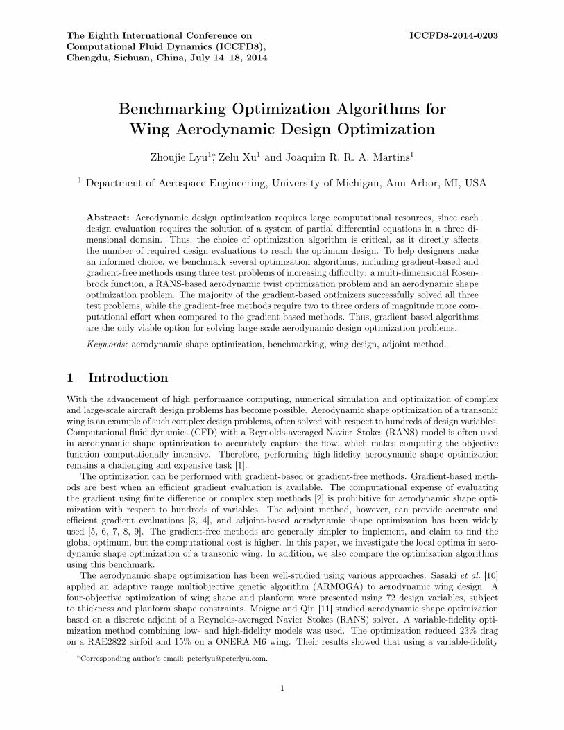
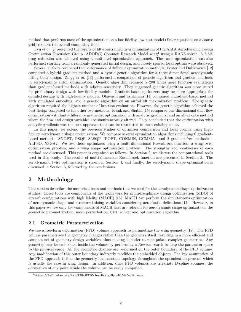
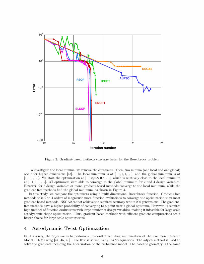
Figure 1 shows the optimization path taken by each optimizer. Gradient-based methods follow throughthe Rosenbrock valley and converge toward the optimum. Gradient-free methods converge their populationtoward the optimum in a more scattered way. The convergence history of selected optimizers of the twodimensional Rosenbrock function is plotted in Figure 2. For gradient-free methods, only the best point isplotted for each iteration or generation. Most of the gradient-based optimizers converge to an objectivetolerance of 10−5 within 150 iterations, while ALPSO converges to the same tolerance using 3, 368 iterationsand NSGA2 can not converge to the same tolerance before we terminate the computation. NSGA2 termi-nates when the maximum number of generation (200) is reached. SLSQP is the fastest, with 34 functionevaluations.

20

20

20

20

1000

1000

1000

1000

8000

8000

8000

x1

x2

­6 ­3 0 3 6­6

­3

0

3

6

20

20

20

20

1000

1000

1000

1000

8000

8000

8000

8000

x1

x2

­6 ­3 0 3 6­6

­3

0

3

6

20

2020

1000

1000

1000

1000

8000

8000

8000

800

0

x1

x2

­6 ­3 0 3 6­6

­3

0

3

6

Infeasible

Feasible

Infeasible

Feasible

20

20

20

20

1000

1000

1000

1000

8000

800

0

8000

8000

x1

x2

­6 ­3 0 3 6­6

­3

0

3

6

Infeasible

Feasible Feasible

20

20

20

1000

1000

1000

1000

8000

800

08000

x1

x2

­6 ­3 0 3 6­6

­3

0

3

6

Infeasible

Feasible

20

20

20

1000

1000

10001

000

8000

8000

8000

80

00

x1

x2

­6 ­3 0 3 6­6

­3

0

3

6

20

20

20

20

1000

1000

1000

1000

8000

80

00

8000

800

0

x1

x2

­6 ­3 0 3 6­6

­3

0

3

6

Infeasible

Feasible

Infeasible

Feasible

20

20

20

20

1000

1000

1000

1000

8000

8000

8000

x1

x2

­6 ­3 0 3 6­6

­3

0

3

6

Infeasible

Feasible

SNOPT

Func eval = 42SLSQP

Func eval = 34

PSQP

Func eval = 39

IPOPT

Func eval = 59

CONMIN

Func eval = 178

GCMMA

Func eval = 3354

ALPSO

Func eval = 3368

NSGA2

Func eval = 4800

Figure 1: Optimization paths for the constrained 2D Rosenbrock function

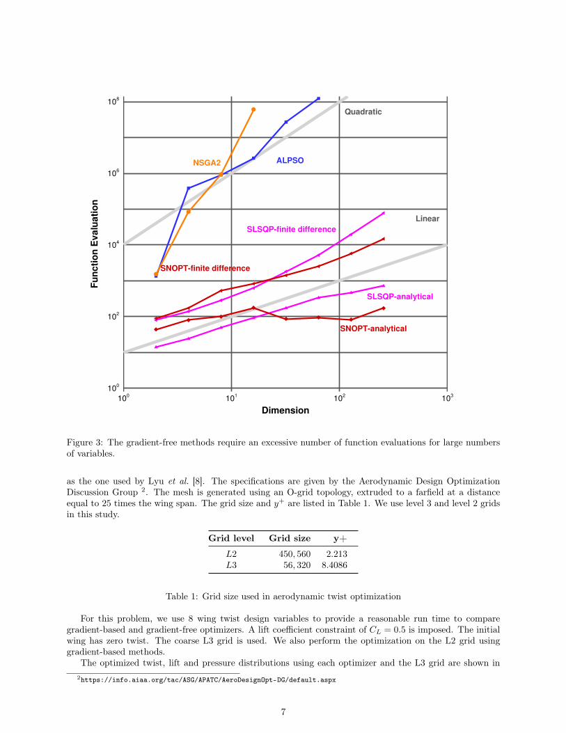
To visualize the effect of increasing the dimensionality of the problem, we also plot the number of functionevaluations required to converge the optimization for an increasing number of design variables. As shownin Figure 3, the gradient-free methods tend to have quadratic or cubic growth of function evaluations withincreasing dimensionality, while the gradient-based methods follow a linear trend. The difference betweengradient-based methods with finite-difference gradients and gradient-based methods with analytical gradientsis significant, motivating the use of the adjoint method in aerodynamic shape optimization that we discusslater.

5

Iteration number

Err

or

100

101

102

103

104

10­15

10­10

10­5

100

105

ALPSO

NSGA2

PSQP

SLSQP

SNOPT

IPOPT

Figure 2: Gradient-based methods converge faster for the Rosenbrock problem

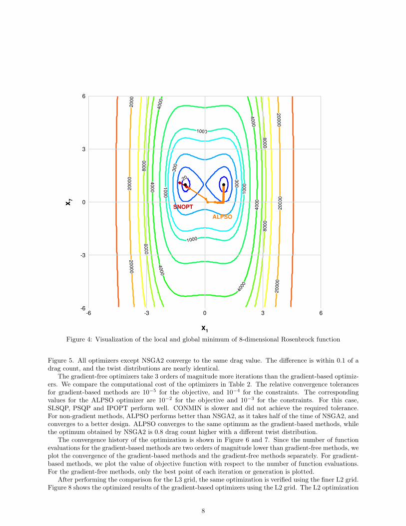
To investigate the local minima, we remove the constraint. Then, two minima (one local and one global)occur for higher dimensions [43]. The local minimum is at [−1, 1, 1, . . .], and the global minimum is at[1, 1, 1, . . .]. We start the optimization at [−0.8, 0.8, 0.8, . . .], which is relatively close to the local minimumat [−1, 1, 1, . . .]. All optimizers were able to converge to the global minimum for 2 and 4 design variables.However, for 8 design variables or more, gradient-based methods converge to the local minimum, while thegradient-free methods find the global minimum, as shown in Figure 4.

In this study, we compare the optimizers using a multi-dimensional Rosenbrock function. Gradient-freemethods take 2 to 4 orders of magnitude more function evaluations to converge the optimization than mostgradient-based methods. NSGA2 cannot achieve the required accuracy within 200 generations. The gradient-free methods have a higher probability of converging to a point near a global optimum. However, it requireshigh number of function evaluations with large number of design variables, making it infeasible for large-scaleaerodynamic shape optimization. Thus, gradient-based methods with efficient gradient computations are abetter choice for large-scale optimizations.

4 Aerodynamic Twist OptimizationIn this study, the objective is to perform a lift-constrained drag minimization of the Common ResearchModel (CRM) wing [44, 45, 46]. The flow is solved using RANS equations. The adjont method is used tosolve the gradients including the linearization of the turbulence model. The baseline geometry is the same

6

Dimension

Fu

nc

tio

n E

va

lua

tio

n

100

101

102

103

100

102

104

106

108

NSGA2 ALPSO

SLSQP­finite difference

SLSQP­analytical

SNOPT­analytical

SNOPT­finite difference

Quadratic

Linear

Figure 3: The gradient-free methods require an excessive number of function evaluations for large numbersof variables.

as the one used by Lyu et al. [8]. The specifications are given by the Aerodynamic Design OptimizationDiscussion Group 2. The mesh is generated using an O-grid topology, extruded to a farfield at a distanceequal to 25 times the wing span. The grid size and y+ are listed in Table 1. We use level 3 and level 2 gridsin this study.

Grid level Grid size y+

L2 450, 560 2.213L3 56, 320 8.4086

Table 1: Grid size used in aerodynamic twist optimization

For this problem, we use 8 wing twist design variables to provide a reasonable run time to comparegradient-based and gradient-free optimizers. A lift coefficient constraint of CL = 0.5 is imposed. The initialwing has zero twist. The coarse L3 grid is used. We also perform the optimization on the L2 grid usinggradient-based methods.

The optimized twist, lift and pressure distributions using each optimizer and the L3 grid are shown in2https://info.aiaa.org/tac/ASG/APATC/AeroDesignOpt-DG/default.aspx

7

20300

30

0

10

00

1000

10

00

1000

4000

40

00

4000

4000

40

00

40

00

80

00

80

00

80

00

80

00

20

00

0

20

00

02

00

00

20

00

02

00

00

20

00

0

x1

x7

­6 ­3 0 3 6­6

­3

0

3

6

SNOPT

ALPSO

Figure 4: Visualization of the local and global minimum of 8-dimensional Rosenbrock function

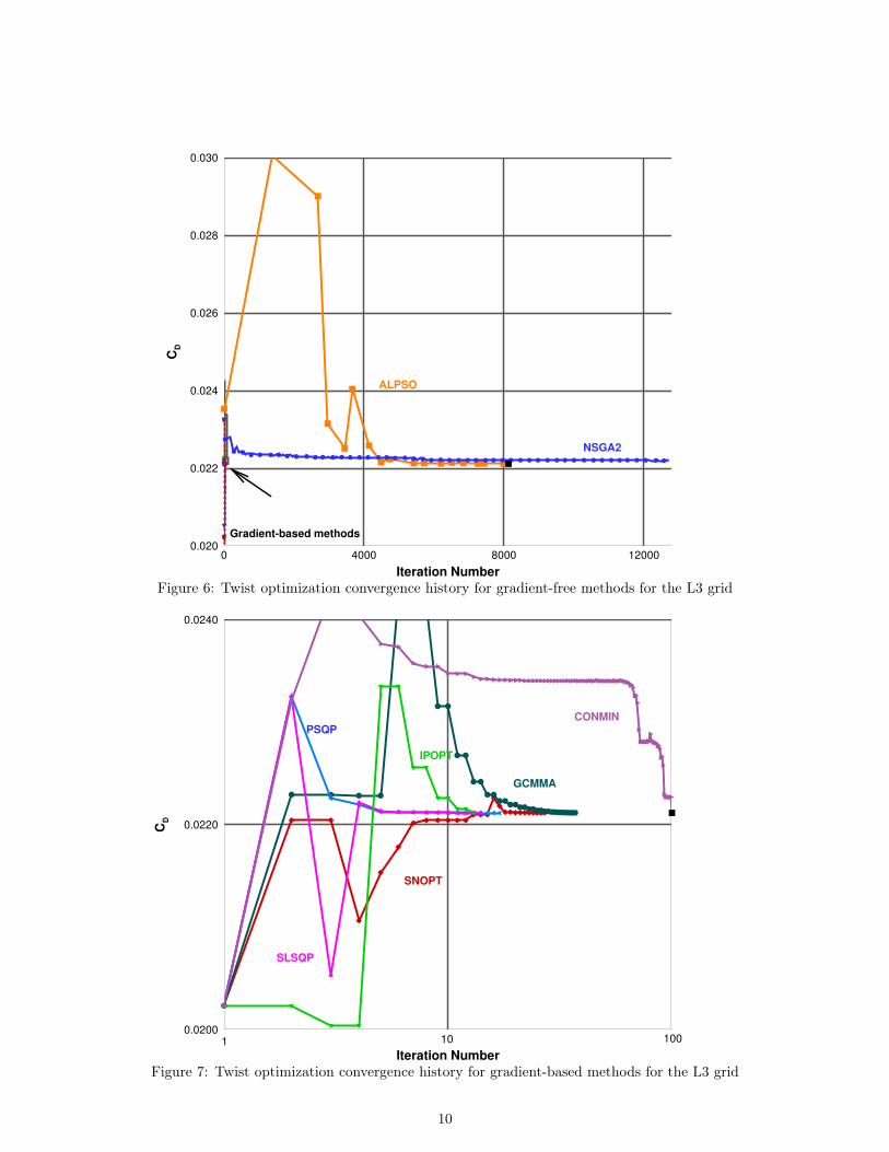
Figure 5. All optimizers except NSGA2 converge to the same drag value. The difference is within 0.1 of adrag count, and the twist distributions are nearly identical.

The gradient-free optimizers take 3 orders of magnitude more iterations than the gradient-based optimiz-ers. We compare the computational cost of the optimizers in Table 2. The relative convergence tolerancesfor gradient-based methods are 10−5 for the objective, and 10−4 for the constraints. The correspondingvalues for the ALPSO optimizer are 10−2 for the objective and 10−3 for the constraints. For this case,SLSQP, PSQP and IPOPT perform well. CONMIN is slower and did not achieve the required tolerance.For non-gradient methods, ALPSO performs better than NSGA2, as it takes half of the time of NSGA2, andconverges to a better design. ALPSO converges to the same optimum as the gradient-based methods, whilethe optimum obtained by NSGA2 is 0.8 drag count higher with a different twist distribution.

The convergence history of the optimization is shown in Figure 6 and 7. Since the number of functionevaluations for the gradient-based methods are two orders of magnitude lower than gradient-free methods, weplot the convergence of the gradient-based methods and the gradient-free methods separately. For gradient-based methods, we plot the value of objective function with respect to the number of function evaluations.For the gradient-free methods, only the best point of each iteration or generation is plotted.

After performing the comparison for the L3 grid, the same optimization is verified using the finer L2 grid.Figure 8 shows the optimized results of the gradient-based optimizers using the L2 grid. The L2 optimization

8

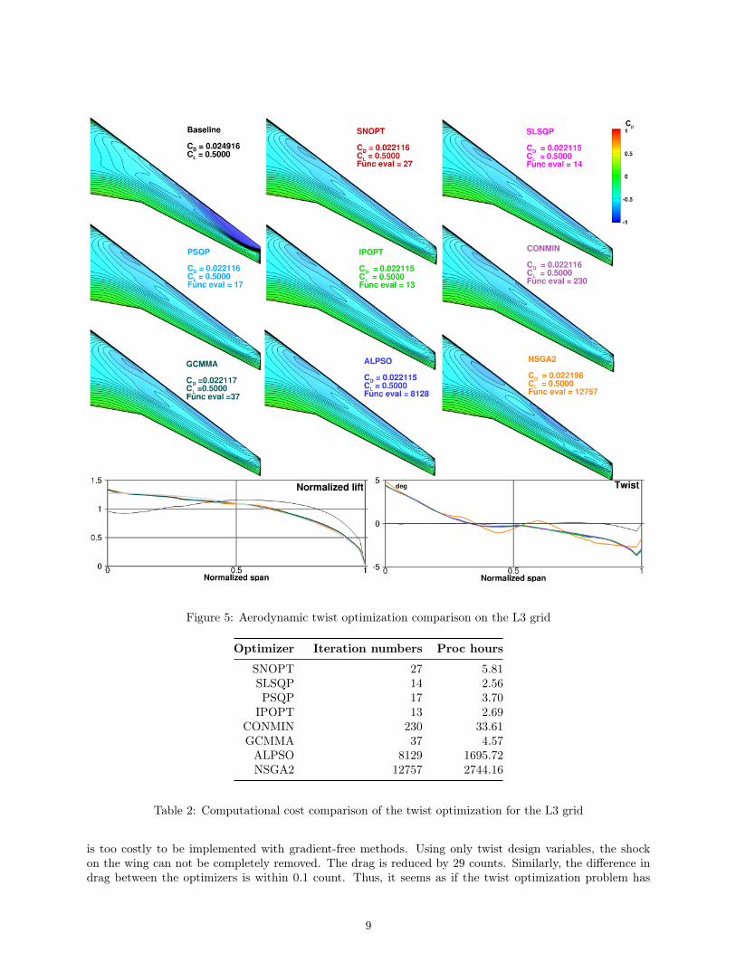
Figure 5: Aerodynamic twist optimization comparison on the L3 grid

Optimizer Iteration numbers Proc hours

SNOPT 27 5.81SLSQP 14 2.56PSQP 17 3.70

IPOPT 13 2.69CONMIN 230 33.61GCMMA 37 4.57ALPSO 8129 1695.72NSGA2 12757 2744.16

Table 2: Computational cost comparison of the twist optimization for the L3 grid

is too costly to be implemented with gradient-free methods. Using only twist design variables, the shockon the wing can not be completely removed. The drag is reduced by 29 counts. Similarly, the difference indrag between the optimizers is within 0.1 count. Thus, it seems as if the twist optimization problem has

9

Iteration Number

CD

0 4000 8000 120000.020

0.022

0.024

0.026

0.028

0.030

ALPSO

NSGA2

Gradient­based methods

Figure 6: Twist optimization convergence history for gradient-free methods for the L3 grid

Iteration Number

CD

0.0200

0.0220

0.0240

SNOPT

IPOPT

CONMIN

SLSQP

PSQP

GCMMA

1 10 100

Figure 7: Twist optimization convergence history for gradient-based methods for the L3 grid

10

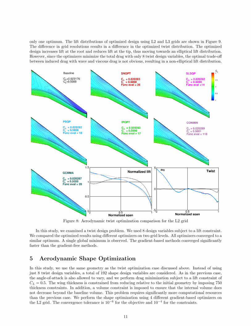
only one optimum. The lift distributions of optimized design using L2 and L3 grids are shown in Figure 9.The difference in grid resolutions results in a difference in the optimized twist distribution. The optimizeddesign increases lift at the root and reduces lift at the tip, thus moving towards an elliptical lift distribution.However, since the optimizers minimize the total drag with only 8 twist design variables, the optimal trade-offbetween induced drag with wave and viscous drag is not obvious, resulting in a non-elliptical lift distribution.

Figure 8: Aerodynamic twist optimization comparison for the L2 grid

In this study, we examined a twist design problem. We used 8 design variables subject to a lift constraint.We compared the optimized results using different optimizers on two grid levels. All optimizers converged to asimilar optimum. A single global minimum is observed. The gradient-based methods converged significantlyfaster than the gradient-free methods.

5 Aerodynamic Shape OptimizationIn this study, we use the same geometry as the twist optimization case discussed above. Instead of usingjust 8 twist design variables, a total of 192 shape design variables are considered. As in the previous case,the angle-of-attack is also allowed to vary, and we perform drag minimization subject to a lift constraint ofCL = 0.5. The wing thickness is constrained from reducing relative to the initial geometry by imposing 750thickness constraints. In addition, a volume constraint is imposed to ensure that the internal volume doesnot decrease beyond the baseline volume. This problem requires significantly more computational resourcesthan the previous case. We perform the shape optimization using 4 different gradient-based optimizers onthe L2 grid. The convergence tolerance is 10−6 for the objective and 10−4 for the constraints.

11

Normalized Span

Tw

ist

0 0.5 1­5.0

0.0

5.0

L2 Optimized

L3 OptimizedBaseline

deg

No

rma

lize

d L

ift

0.0

0.5

1.0

1.5

L2 Baseline

L2 Optimized

L3 Optimized

L3 BaselineElliptical

Figure 9: Lift distribution comparison of the twist optimized designs

Figure 10 shows the final design resulting from the use of different optimizers. The results from thebaseline wing are shown in black. More detailed comparisons for each optimizer are shown in Figures 12– 15.The drag is reduced by 4.84%, from 206.7 to 196.6 counts, which is similar to the previous result [8].

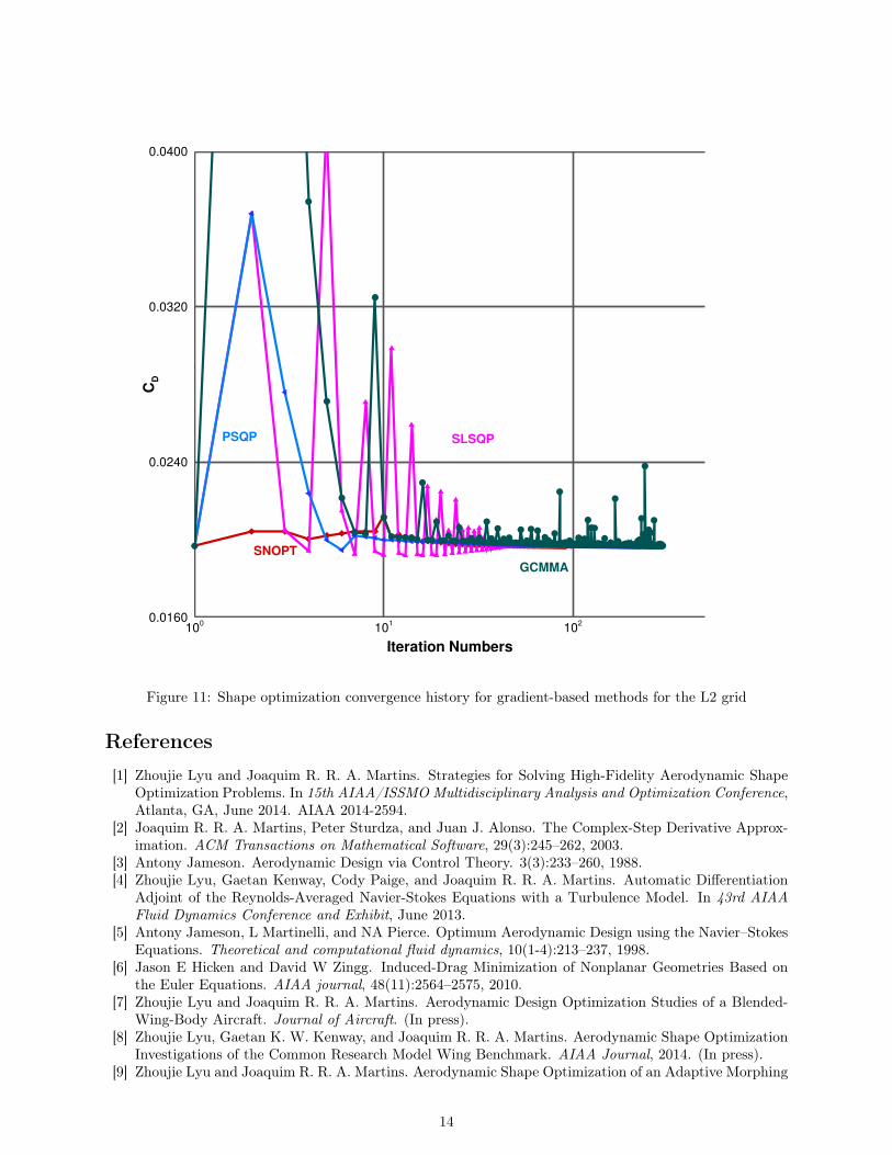
We can see that all optimizers achieve a shock-free wing with an elliptical lift distribution. The baselinedesign has a strong shock, as evidenced by closely spaced Cp contours, while the optimized designs have aparallel, equally spaced pressure contours. The variation in CD is within 1 drag count between the variousoptimizers. All optimized shapes are similar to each other, and only small difference in shape are observed.The comparison of the computational time for various optimizers is shown in Table 3. SNOPT convergesthe fastest among all optimizers. The optimized results using GCMMA is 0.2 drag count higher than theothers. The convergence history is plotted in Figure 11.

12

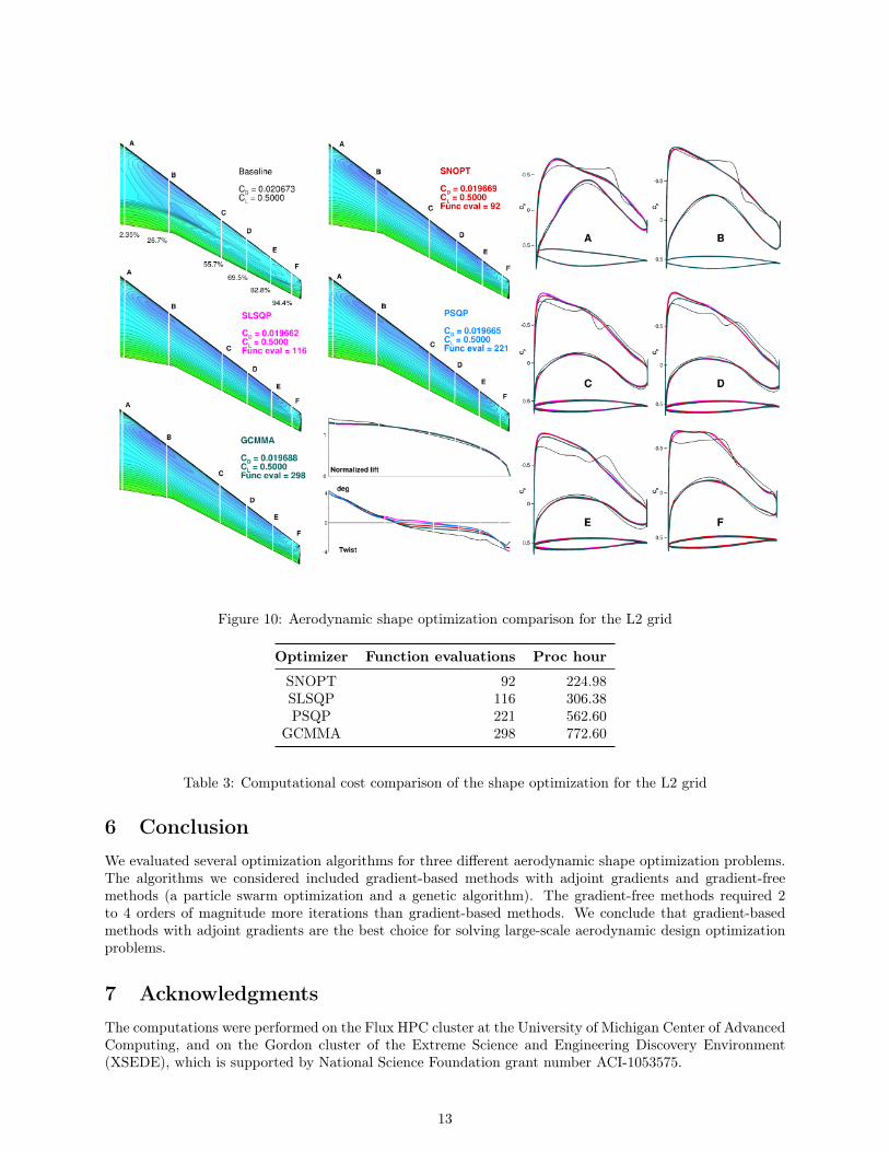
Figure 10: Aerodynamic shape optimization comparison for the L2 grid

Optimizer Function evaluations Proc hour

SNOPT 92 224.98SLSQP 116 306.38PSQP 221 562.60

GCMMA 298 772.60

Table 3: Computational cost comparison of the shape optimization for the L2 grid

6 ConclusionWe evaluated several optimization algorithms for three different aerodynamic shape optimization problems.The algorithms we considered included gradient-based methods with adjoint gradients and gradient-freemethods (a particle swarm optimization and a genetic algorithm). The gradient-free methods required 2to 4 orders of magnitude more iterations than gradient-based methods. We conclude that gradient-basedmethods with adjoint gradients are the best choice for solving large-scale aerodynamic design optimizationproblems.

7 AcknowledgmentsThe computations were performed on the Flux HPC cluster at the University of Michigan Center of AdvancedComputing, and on the Gordon cluster of the Extreme Science and Engineering Discovery Environment(XSEDE), which is supported by National Science Foundation grant number ACI-1053575.

13

Iteration Numbers

CD

100

101

102

0.0160

0.0240

0.0320

0.0400

SLSQPPSQP

SNOPT

GCMMA

Figure 11: Shape optimization convergence history for gradient-based methods for the L2 grid

References[1] Zhoujie Lyu and Joaquim R. R. A. Martins. Strategies for Solving High-Fidelity Aerodynamic Shape

Optimization Problems. In 15th AIAA/ISSMO Multidisciplinary Analysis and Optimization Conference,Atlanta, GA, June 2014. AIAA 2014-2594.

[2] Joaquim R. R. A. Martins, Peter Sturdza, and Juan J. Alonso. The Complex-Step Derivative Approx-imation. ACM Transactions on Mathematical Software, 29(3):245–262, 2003.

[3] Antony Jameson. Aerodynamic Design via Control Theory. 3(3):233–260, 1988.[4] Zhoujie Lyu, Gaetan Kenway, Cody Paige, and Joaquim R. R. A. Martins. Automatic Differentiation

Adjoint of the Reynolds-Averaged Navier-Stokes Equations with a Turbulence Model. In 43rd AIAAFluid Dynamics Conference and Exhibit, June 2013.

[5] Antony Jameson, L Martinelli, and NA Pierce. Optimum Aerodynamic Design using the Navier–StokesEquations. Theoretical and computational fluid dynamics, 10(1-4):213–237, 1998.

[6] Jason E Hicken and David W Zingg. Induced-Drag Minimization of Nonplanar Geometries Based onthe Euler Equations. AIAA journal, 48(11):2564–2575, 2010.

[7] Zhoujie Lyu and Joaquim R. R. A. Martins. Aerodynamic Design Optimization Studies of a Blended-Wing-Body Aircraft. Journal of Aircraft. (In press).

[8] Zhoujie Lyu, Gaetan K. W. Kenway, and Joaquim R. R. A. Martins. Aerodynamic Shape OptimizationInvestigations of the Common Research Model Wing Benchmark. AIAA Journal, 2014. (In press).

[9] Zhoujie Lyu and Joaquim R. R. A. Martins. Aerodynamic Shape Optimization of an Adaptive Morphing

14

Trailing Edge Wing. In 15th AIAA/ISSMO Multidisciplinary Analysis and Optimization Conference,Atlanta, GA, June 2014. AIAA 2014-3275.

[10] Daisuke Sasaki, Masashi Morikawa, Shigeru Obayashi, and Kazuhiro Nakahashi. Aerodynamic ShapeOptimization of Supersonic Wings by Adaptive Range Multiobjective Genetic Algorithms. pages 639–652, 2001.

[11] Alan Le Moigne and Ning Qin. Variable-Fidelity Aerodynamic Optimization for Turbulent Flows usinga Discrete Adjoint Formulation. AIAA Journal, 42(7):1281–1292, 2004.

[12] Norman F Foster and George S Dulikravich. Three-Dimensional Aerodynamic Shape Optimizationusing Genetic and Gradient Search Algorithms. Journal of Spacecraft and Rockets, 34(1):36–42, 1997.

[13] D. W. Zingg, M. Nemec, and T. H. Pulliam. A Comparative Evaluation of Genetic and Gradient-BasedAlgorithms Applied to Aerodynamic Optimization. European Journal of Computational Mechanics,17(1–2):103–126, January 2008.

[14] Shigeru Obayashi and Takanori Tsukahara. Comparison of Optimization Algorithms for AerodynamicShape Design. AIAA journal, 35(8):1413–1415, 1997.

[15] Paul D Frank and Gregory R Shubin. A Comparison of Optimization-Based Approaches for a ModelComputational Aerodynamics Design Problem. Journal of Computational Physics, 98(1):74–89, 1992.

[16] Gaetan K. W. Kenway, Graeme J. Kennedy, and Joaquim R. R. A. Martins. Scalable Parallel Approachfor High-Fidelity Steady-State Aeroelastic Analysis and Adjoint Derivative Computations. AIAA Jour-nal, 52(5):935–951, 2014.

[17] Gaetan K. W. Kenway and Joaquim R. R. A. Martins. Multipoint High-Fidelity Aerostructural Opti-mization of a Transport Aircraft Configuration. Journal of Aircraft, 51(1):144–160, 2014.

[18] Gaetan KWKenway, Graeme J Kennedy, and J. R. R. A. Martins. A Cad-free Approach to High-FidelityAerostructural Optimization. In Proceedings of the 13th AIAA/ISSMO Multidisciplinary Analysis Op-timization Conference, Fort Worth, TX, 2010.

[19] Edwin van der Weide, Georgi Kalitzin, Jorg Schluter, and Juan Alonso. Unsteady TurbomachineryComputations Using Massively Parallel Platforms. In 44th AIAA Aerospace Sciences Meeting andExhibit, 2006.

[20] A Jameson, Wolfgang Schmidt, and Eli Turkel. Numerical Solution of the Euler Equations by Finite Vol-ume Methods using Runge Kutta Time Stepping Schemes. In 14th AIAA, Fluid and Plasma DynamicsConference, 1981.

[21] Charles A. Mader, Joaquim R. R. A. Martins, Juan J. Alonso, and Edwin van der Weide. ADjoint: AnApproach for the Rapid Development of Discrete Adjoint Solvers. AIAA Journal, 46(4):863–873, April2008.

[22] Youcef Saad and Martin H Schultz. GMRES: A Generalized Minimal Residual Algorithm for SolvingNonsymmetric Linear Systems. SIAM Journal on Scientific and Statistical Computing, 7(3):856–869,1986.

[23] Satish Balay, William D. Gropp, Lois Curfman McInnes, and Barry F. Smith. Efficient Managementof Parallelism in Object Oriented Numerical Software Libraries. In E. Arge, A. M. Bruaset, and H. P.Langtangen, editors, Modern Software Tools in Scientific Computing, pages 163–202. Birkhäuser Press,1997.

[24] Satish Balay, Jed Brown, , Kris Buschelman, Victor Eijkhout, William D. Gropp, Dinesh Kaushik,Matthew G. Knepley, Lois Curfman McInnes, Barry F. Smith, and Hong Zhang. PETSc Users Manual.Technical Report ANL-95/11 - Revision 3.4, Argonne National Laboratory, 2013.

[25] Satish Balay, Jed Brown, Kris Buschelman, William D. Gropp, Dinesh Kaushik, Matthew G.Knepley, Lois Curfman McInnes, Barry F. Smith, and Hong Zhang. PETSc Web Page, 2013.http://www.mcs.anl.gov/petsc.

[26] Charles A. Mader and Joaquim R. R. A. Martins. Stability-Constrained Aerodynamic Shape Optimiza-tion of Flying Wings. Journal of Aircraft, 50(5):1431–1449, September 2013.

[27] Zhoujie Lyu and Joaquim R. R. A. Martins. Aerodynamic Shape Optimization of a Blended-Wing-BodyAircraft. In 51st AIAA Aerospace Sciences Meeting including the New Horizons Forum and AerospaceExposition, 2013.

[28] Rhea P. Liem, Gaetan K. W. Kenway, and Joaquim R. R. A. Martins. Multi-Mission Aircraft FuelBurn Minimization via Multi-Point Aerostructural Optimization. AIAA Journal, 2014. (Submitted).

[29] Ruben E. Perez, Peter W. Jansen, and Joaquim R. R. A. Martins. pyOpt: A Python-Based Object-

15

Oriented Framework for Nonlinear Constrained Optimization. Structures and Multidisciplinary Opti-mization, 45(1):101–118, 2012.

[30] Philip E Gill, Walter Murray, and Michael A Saunders. SNOPT: An SQP Algorithm for Large-ScaleConstrained Optimization. SIAM journal on optimization, 12(4):979–1006, 2002.

[31] Dieter Kraft. A Software Package for Sequential Quadratic Programming. Technical report, Tech. Rep.DFVLR-FB 88-28, DLR German Aerospace Center, 1988.

[32] Charles L Lawson and Richard J Hanson. Solving Least Squares Problems, volume 161. SIAM, 1974.[33] Dieter Kraft. Algorithm 733: TOMP–Fortran Modules for Optimal Control Calculations. ACM Trans-

actions on Mathematical Software (TOMS), 20(3):262–281, 1994.[34] Andreas Wächter and Lorenz T Biegler. On the Implementation of an Interior-Point Filter Line-Search

Algorithm for Large-Scale Nonlinear Programming. Mathematical programming, 106(1):25–57, 2006.[35] Garret N Vanderplaats. CONMIN, a FORTRAN Program for Constrained Function Minimization:

User’s Manual, volume 62282. Ames Research Center and US Army Air Mobility R&D Laboratory,1973.

[36] Krister Svanberg. The Method of Moving Asymptotes–a New Method for Structural Optimization.International journal for numerical methods in engineering, 24(2):359–373, 1987.

[37] P. W. Jansen and R. E. Perez. Constrained Structural Design Optimization via a Parallel AugmentedLagrangian Particle Swarm Optimization Approach. Computers & Structures, 89(13–14):1352–1366, 72011.

[38] RE Perez and K Behdinan. Particle Swarm Approach for Structural Design Optimization. Computers& Structures, 85(19):1579–1588, 2007.

[39] Peter Jansen, Ruben. E. Perez, and Joaquim R. R. A. Martins. Aerostructural Optimization of Non-planar Lifting Surfaces. Journal of Aircraft, 47(5):1491–1503, 2010.

[40] Sohrab Haghighat, Joaquim R. R. A. Martins, and Hugh H. T. Liu. Aeroservoelastic Design Optimiza-tion of a Flexible Wing. Journal of Aircraft, 49(2):432–443, 2012.

[41] K. Deb, A. Pratap, S. Agarwal, and T. Meyarivan. A Fast and Elitist Multiobjective Genetic Algorithm:NSGA-II. Evolutionary Computation, IEEE Transactions on, 6(2):182–197, 2002.

[42] H. H. Rosenbrock. An Automatic Method for Finding the Greatest or Least Value of a Function. TheComputer Journal, 3(3):175–184, 1960.

[43] Jorge J Moré, Burton S Garbow, and Kenneth E Hillstrom. Testing Unconstrained OptimizationSoftware. ACM Transactions on Mathematical Software (TOMS), 7(1):17–41, 1981.

[44] J. Vassberg. Introduction: Drag Prediction Workshop. Journal of Aircraft, 45(3):737–737, Jun 2008.[45] John Vassberg, Mark Dehaan, Melissa Rivers, and Richard Wahls. Development of a Common Research

Model for Applied CFD Validation Studies. In 26th AIAA Applied Aerodynamics Conference. AmericanInstitute of Aeronautics and Astronautics, August 2008.

[46] John Vassberg. A Unified Baseline Grid about the Common Research Model Wing/Body for the FifthAIAA CFD Drag Prediction Workshop (Invited). In 29th AIAA Applied Aerodynamics Conference, Jul2011.

16

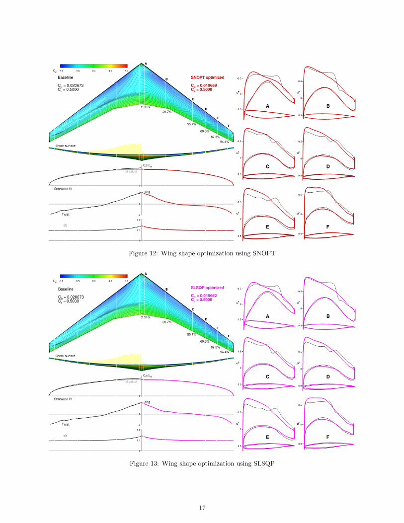
Figure 12: Wing shape optimization using SNOPT

Figure 13: Wing shape optimization using SLSQP

17

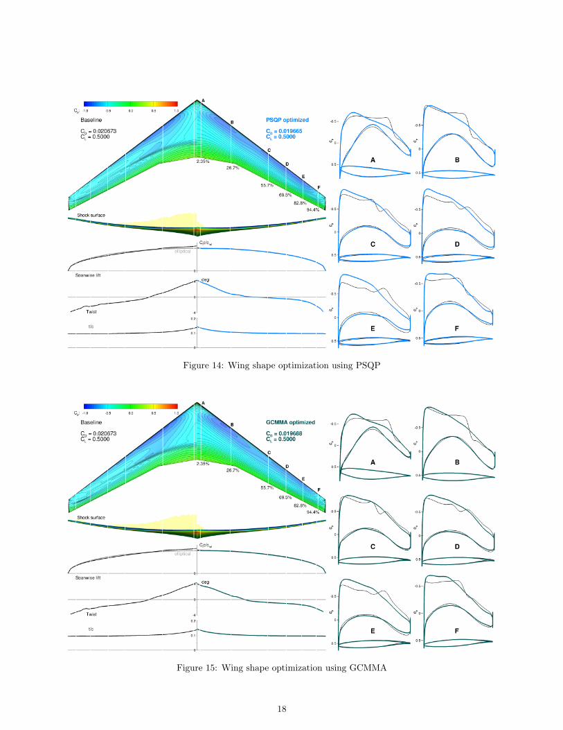
Figure 14: Wing shape optimization using PSQP

Figure 15: Wing shape optimization using GCMMA

18