bellotime frequency duality

18 IEEE TRANSACTIONS ON INFORMATION THEORY January

Time-Frequency Duality* PHILLIP BELLOt, SENIOR MEMBER, IEEE

Summary-This paper develops a concept of duality, called time-frequency duality, which is applicable to a class of networks called communication-signal-processing networks. Such networks consist of an interconnection of basic elements such as filters, mixers, delay lines, etc. The usefulness of time-frequency duality stems from the fact that two situations which may be quite distinct physically can have identical behavior patterns except for an interchange of the roles played by time and frequency. As a result, the solution to a detection or estimation problem may be found directly from the solution of the dual problem, if known, merely by replacing variables and quantities by their duals. This application of time-frequency duality is illustrated in the paper by the problem of measuring the transfer function of a scatter medium by means of an optimal gating operation prior to spectrum analysis.

Another benefit to be obtained from time-frequency duality is the generation of new ideas for communication signal processing techniques. We illustrate this type of benefit by constructing the dual of the Kineplex communication system.

A thiid benefit is the additional insight gained into a communication problem by the ability to look at it in another way. This benefit is illustrated by the characterization of time-variant linear channels. It is demonstrated that such channels may be characterized in an interesting symmetrical manner in time and frequency variables by defining dual system functions.

I. INTRODUCTION

T

HE CONCEPT OF duality has proved quite useful in the analysis and synthesis of lumped electrical networks. This usefulness stems from the fact that

two situations, which are entirely analogous on a current and voltage basis, respectively, have identical behavior patterns, except for an interchange of the roles played by voltage and current, while physically and geometrically they are distinctly different. Thus, a means is provided for recognizing the analytical equivalence of pairs of physically dissimilar networks or, conversely, for devising two geometrically different ways of interpreting a given situation.

To the communication engineer, the words “time” and “frequency” connote complementary concepts. This connotation has arisen from the Fourier transform relationship between a time function and its spectrum and the extensive shuttling between the time and frequency domains which takes place in the solution of many communication problems. It is fair to say that a concept of ‘(time-frequency” duality has existed previously, although on a rather undefined plane. We shall form a more precise concept of time-frequency duality, one which will provide the communication engineer with the same type of benefits that duality provides in the study of lumped electrical networks. Although the same degree of usefulness may not result from the application of time-frequency duality concepts as from the application

* Received October 5, 1962. t ADCOM, Inc., 238 Main Street, Cambridge, Mass.

of voltage-current duality, the concept of time-frequency duality as developed here is sufficiently interesting and useful to warrant at least the brief treatment given in this paper.

Throughout this paper we shall deal with complex time functions and their spectra and with complex “low-pass” equivalent filters. Such an approach is used not only because the full flavor of time-frequency duality appears in such a context, but also, as discussed below, because narrow-band processes and channels whose inputs and outputs are narrow-band processes are most simply described thereby.

II. COMPLEX ENVELOPES A process z(t) whose spectral components cover a

band of frequencies which is small compared to any frequency in the band may be expressed as

x(t) = Re {z(t)eiU”“) (1)

where Re { ) is the usual real part notation, w0 is some (angular) frequency within the band, and x(t) is the complex envelope of s(t). This name for x(t) derives from the fact that the magnitude of x(t) is the conventional envelope of z(t), while the angle of x(t) is the conventional phase of x(t) measured with respect to carrier phase wet. The non-narrowband case may be handled with the complex notation also by the use of Hilbert transforms [l]-[4]. However, the complex envelope will then no longer have the simple interpretation described above.

Complex envelope notation will be used extensively for the remainder of this paper. However, it should be understood that there is always implied the existence of a center or reference frequency w0 which, via an equation such as (l), converts the complex time functions under discussion into physical narrow-band signals.

The reception of narrow-band signals is usually ac- companied by an additive “white” noise. For purposes of analysis, however, it is not necessary to consider this white noise to be flat over infinite bandwidth. It is sufficient for all practical problems to use an “equivalent” noise which has a .flat power density spectrum only over the range of frequencies that will be processed by the receiver. This range of frequencies is invariably narrow enough so that an equivalent narrow-band noise may be used in place of the white noise. On this basis, we justify the use of complex envelope notation to rep- resent the additive noise. It is readily demonstrated that if the real additive noise has a (two-sided) spectral intensity of N,, then the complex envelope of the “equivalent” low-pass noise has (two-sided) spectral intensity of 4No.

1964 Belle: Time Frequency Duality 19

When dealing with problems in which there are wide- band filters (time variant included) whose inputs and outputs are narrow-band (when expressed with reference to the same center frequency), it is possible to replace these filters with equivalent narrow-band filters which leave the input-output relations invariant. This fact becomes obvious when it is realized that by preceding and following a wide-band filter with narrow-band filters which have flat transfer functions over the range of input and output frequencies of interest, one produces a com- posite filter which is narrow-band and, of course, cannot change the input-output relations for the properly re- stricted class of input and output narrow-band signals. It is readily demonstrated that (except for an unimportant constant of one half) the complex envelope of a narrow- band signal at the output of a narrow-band filter due to a narrow-band input may be obtained by passing the complex envelope of the input through an equivalent low-pass filter whose impulse response is just equal to the complex envelope of the narrow-band filter impulse response.

In defining the autocorrelation function of the complex envelope of a random process, a certain difficulty appears that is not generally appreciated, namely, that two autocorrelation functions are needed in order to uniquely specify the autocorrelation function of the original real process. This fact is demonstrated by direct calculation of the autocorrelation function of z(t), (I), as

x(t)z(s) = 4 Re (x*(t)x(s)eYwO(‘--I)J -

+ $ Re (.z(t)z(s)e’““(S+t) 1.

(2)

Thus, the two autocorrelation functions

r(t, s) = x*(t)%(s) (3)

qt, s) = z(t)x(s)

are needed to specify the autocorrelation function of the real process. Fortunately, in most applications’ the narrow-band process is so constituted that

F(t, s) = 0. (4)

In fact, from (2), one may readily deduce that (4) is necessary if z(t) is to be wide sense stationary.

A simple physical test of a(t) (determinist,ic components removed) to d&ermine whet’her (4) is satisfied is to mul- tiply it by it’self delayed and examine l-he sum frequency component for the presence of a deterministic component. According t’o (2) the complex amplitude of t,his component is +?(t, s) so that the presence of a deterministic component would mean that (4) is violated. In the subsequent discussion we shall deal only with r(t, s) when the autocorrelation function of a complex process is under discussion. It should be kept in mind, however, that an analogous discussion applies for ?(t, s) in those cases where it is nonzero.

1 For an exception see Bello [18].

The above discussion of complex envelopes, equivalent noises, and equivalent filters is supplied as a physical justification for our subsequent use of “low-pass” complex time functions, complex white noise, and low-pass filters wit,h complex impulse responses.

III. COMPLEX AMPLITUDE SPECTRA FOR RANDOM PROCESSES

Contrary to popular engineering opinion, one may define and use to advantage complex amplitude spectra in addition to power spectra when dealing with random processes. The rigorous basis for such use has existed for some time in the more abstract measure-theoretic * books on statistics [5]-[7]. In this rigorous formulation the Fourier-Stieltjes transform plays a central role. However, a heuristic approach employing the ordinary Fourier transform supplemented by delta functions and white noise has not appeared previously. It is under- standable and logical that one who refuses to deal with delta functions and white noise per se should shy away from the use of complex amplitude spectra for random processes. On the other hand, as will become apparent from subsequent discussion, it is not logical that anyone willing to traffic in 6he use of such concepts as LLwhite” noise and delta functions should refuse to deal with complex amplitude spectra for random processes.

In the following discussion, we shall first deal with the complex amplitude spectra of n.s. (nonstationary) white noise and W.S.S. (wide-sense stationary) noise and then we shall deal with the more general nonstationary non- white noise case.

We define a noise process x(t) as being n.s. white noise if its autocorrelation function has the form

r(t, s) = N(t)6(s - t), (5)

where 6(s - t) is a unit impulse located at s = t and N(t) is a non-negative real function which may be interpreted as a “time-variant” spectral density.

When the white noise is W.S.S. and of (two-sided) power density N,,,

r(t, s) = N&s - t>. (6) It is clear that one may generate a n.s. white noise x(t) with an autocorrelation function of the form of (5) by forming the product

x(t) = 1/N(t)%(t) (7)

where x,,(t) is a W.S.S. white noise of unity spectral density (N, = 1).

One may give a physical interpretation to the complex amplitude spectrum of n.s. white noise in familiar terms by noting that the random variable defining this spectrum at specified frequencies is interpretable as the t = 0 response of a time invariant linear filter to W.S.S. white noise of unity spectral density. Thus if Z(f) denotes the spectrum of z(t) in (7) then

Z(f) = 1 2f(t)e-iar’t --

dt = [x0(t) @ dN(-t)e’Zff’t]t=o (8)

20 IEEE TRANSACTIONS ON INFORMATION THEORY

where the symbol @ denotes convolution. Changing the frequency at which the spectrum is evaluated from f to 1, say, changes the filter impulse response from dN(- t) e izaft to ~jq-qei2”lt. Thus the autocorrelation function of the spectrum R(f, I),

January

noise is also W.S.S. and white with numerically identical power density, N,.

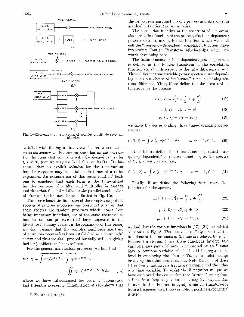
We have demonstrated, heuristically, the existence of complex amplitude spectra for the cases of W.S.S. noise and n.s. white noise. As diagrammed in Fig. l(a), the former type of noise may be generated by passing W.S.S. white noise through a linear time invariant filter, while the latter type of noise may be generated by multiplying W.S.S. white noise by an appropriate deterministic waveform.

Wf, 0 = z*(f>m, (9) may be directly interpreted as the cross-correlation between the outputs of two time invariant filters at t = 0 when the two filters have a common W.S.S. white noise input of unity spectral density.

This autocorrelation function is given by

R(f, Z) = 11 eizs(‘t-ia) z/N(t)N(s)

where

-- *x%(t)&) dt ds = R(Z - f), (10)

R(Q) = / em”* ‘“N(t) dt. (11)

Since the autocorrelation function of the complex amplitude spectrum of n.s. white noise is a function only of the difference I;t = I - f, this spectrum is W.S.S. (in the frequency variable). Note also that R(Q), the resulting autocorrelation function, is just equal to the Fourier transform of the “time-dependent” spectral density N(t).

At this point in our discussion, we would like to state an obvious fact: The properties of x(t) and Z(f) discussed above do not depend on the variables t and f; rather, they are the properties of a function x( .) and its Fourier transform Z(a), where we have put dots in place of the variables t and f to emphasize the fact that any pair of variables may be used.

Because of the symmetry of the direct and inverse Fourier transform, we must conclude immediately from the above ahnost trivial observation that the not so trivial conclusion that a W.S.S. random process x(t) with autocorrelation function

-- 2~(t)x(s) = r(s -

must have a complex amplitude autocorrelation function

z*(f)m) = nf)a

0 (12)

spectrum Z(f) with

- f> (13)

where

T(T) = I'(f)eizrlr df. s (14)

Thus, the complex amplitude spectrum of W.S.S. noise is a n.s. noise in the frequency variable with a “frequency- dependent” spectral density P(f) just equal to the conventional power spectrum of the stationary noise process.

It is interesting to note that when the process x(t) is W.S.S. and white (B),

z*(f)z(Z) = NoU - f), (15) i.e., the complex amplitude spectrum of W.S.S. white

Consider now the more general random processes of Fig. l(b) which are generated by passing W.S.S. white noise through the filter-multiplier and multiplier-filter cascades or, in other words, by multiplying W.S.S. noise by a deterministic waveform and by passing n.s. white noise through a linear time invariant filter. As may readily be determined, these two types of random processes bear the same relationship as W.S.S. noise and n.s. white noise, namely, the autocorrelation function of the spectrum of one process has the same analytical form as the autocorrelation function of the other process. This equivalence is useful in allowing one to obtain an intuitive grasp of the nature of the complex amplitude spectra of these two classes of random processes. Thus, for example, one may state that the complex amplitude spectrum of filtered n.s. white noise is a random process in the frequency variable which has the character of W.S.S. noise multiplied by a determininistic frequency function (the transfer function of the filter, of course).

Our reason for considering these two types of random processes is that for all practical purposes one may generate an ns. random process with an arbitrarily speciJied autocorrelation function as a sum of processes of either type. Thus, at least as far as correlation properties are concerned, no additional conceptual difficulties arise in dealing with the complex amplitude spectra of general nonstationary processes.

The proof that one may generate a nonstationary process with a specified autocorrelation function as a sum of (possibly dependent) noises, each resulting from the passage of wide-sense stationary white noise through filter-multiplier (or multiplier-filter) cascades, follows directly from a generalization to nonstationary processes of the spectrum-shaping technique of Bode and Shannon [8] and Zadeh and Ragazeini [9]. This generalization is a technique for determining a (nonrandom) time-variant linear filter whose output has a specified correlation function when its input is wide-sense stationary white noise. A rather detailed review of work on this problem has been presented by Zadeh [lo].” While this problem does not appear to have been completely solved in all cases of theoretical interest, it does appear to have a solution for most problems of practical interest where it is only necessary to characterize the random process under consideration over sufficiently large but not infinite time and frequency ranges. Thus, for example, if we are

z L. 9. Zadeh [lo], see Sec. III.


FILTERED N.S. WHITE NC,SE

MULTIPLIED w.s s. NOlSE

TIME FUNCTION

(b)

(cl

Fig. l-Relevant to interpret$i;ti;i complex amplitude spectrum

satisfied with finding a time-variant filter whose wide- sense stationary white noise response has an autocorrelation function that coincides with the desired r(t, s) for t, s < T, then we may use Kailath’s results [II]. He has shown that an explicit solution for the time-variant impulse response may be obtained in terms of a series expansion. An examination of this series solution3 leads one to conclude that each term is the time-variant impulse response of a filter and multiplier in cascade and thus that the desired filter is the parallel combination of filter-multiplier cascades as indicated in Fig. l(c).

The above heuristic discussion of the complex amplitude spectra of random processes was presented to show that these spectra are random processes which, apart from being frequency functions, are of the same character as familiar random processes that have appeared in the literature for many years. In the remainder of this paper, we shall assume that the complex amplitude spectrum of a random process has been established as a meaningful entity and thus we shall proceed formally without giving further justification for its existence.

For the general n.s. random processes, we find that

R(f, 1) = / z*(t)e72a’t dt / z(s)e-i2T1y ds

i2T(ft--lS) = ss r(t, s)e dt ds (16)

where we have interchanged the order of integration and ensemble averaging. Examination of (16) shows that

3 T. Kailath [II], see (6).

the autocorrelation functions of a process and its spectrum are double Fourier Transform pairs.

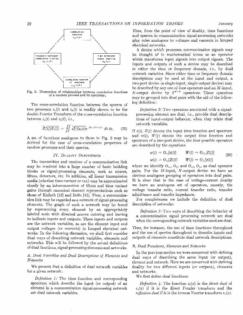
The correlation function of the spectrum of a process, the correlation function of the process, the time-dependeat power-spect.rum, and a fourth function which we shall call the “frequency-dependent” correlation function, have interesting Fourier Transform relationships which are worth developing here.

The instantaneous or time-dependent power spectrum is defined as the Fourier transform of the correlation function r(t, s) with respect to the time difference s - t. Three different time variable power spectra result depending upon our choice of “reference” time in defining the time difference. Thus, if we define the three correlation functions for the process

C”(f, 7) = 1’ (

t - ;: t + ; 1 (17)

c,(f, T) = r(f, t + T) (18)

C-I(t, T) = ,?(t - 7, f) (19)

we have the corresponding t,hree time-dependent power spectra

P,r,(f, t) = / c,,(f, T)e-j’*” dr; 111 = -1, 0, 1. (20)

Now let us define the three functions, called “frequency-dependent” correlation functions, as the spectra of C,n(t, 7) with 7 fixed, i.e.,

C,,,(T, Q) = s c,,,(f, 7)e-jzT 5x dt; na = -l,O, 1. (21)

Finally, if we define the following three correlation functions for the spectra

p,(f, 12) = R ( f - ;: f + 4) (22)

Pl(f, a> = w, f + 0) (23)

P-l(f, Q2) = R(f - $4 f), (24)

we find that the various functions in (17)-(24) are related as shown in Fig. 2. The line labeled F signifies that the functions at the terminals of the line are related by single Fourier transforms. Since these functions involve two variables, any pair of functions connected by an F must have a common variable which should be regarded as fixed in employing the Fourier Transform relationships involving the other two variables. Note that one of these latter two variables is a frequency variable and the other is a time variable. To make the F notation unique we have employed the convention that in transforming from a time to a frequency variable, a negative exponential is used in the Fourier integral, while in transforming from a frequency to a time variable, a positive exponential is used.

22 IEEE TRANXACTIONX ON

Fig. ‘L-Illustration of relationships between correlation functions of a random process and its spectrum i

The cross-correlation function between the spectra of two processes x,(t) and z*(t) is readily shown to be the double Fourier Transform of the cross-correlation function between za(t) and z*(t), i.e.,

Z,*(f)Z,(Z) = /[ xdoz,(s)e i2*(ft-‘s) dt ds. (25)

A set of functions analogous to those in Fig. 2 may be derived for the case of cross-correlation properties of random processes and their spectra.

IV. DUALITY DEFINITIONS The transmitter and receiver of a communication link

may be resolved into a large number of basic building blocks or signal-processing elements, such as mixers, filters, detectors, etc. In addition, all linear transmission media (whether time-variant or not) may be approximated closely by an interconnection of filters and time variant gains through canonical channel representations such as those of Kailath [12] and Bello [13]. Thus, a communication link may be regarded as a network of signal-processing elements. The graph of such a network may be found by representing every element by an appropriately labeled node with directed arrows entering and leaving to indicate inputs and outputs. These inputs and outputs are the network variables, as are the element input and output voltages (or currents) in lumped electrical networks. In the following discussion, we shall first consider dual ways of describing network variables, elements and networks. This will be followed by the actual definitions of dual functions, signal-processing elements and networks.

A. Dual Variables and Dual Descriptions of Elements and Networks

We present first a definition of dual network variables for a given network:

Definition 1: The time function and corresponding spectrum which describe the input (or output) of an element in a communication signal-processing network are dual network variables.

INFORMATION THEORY January

Thus, from the point of view of duality, time functions and spectra in communication signal-processing networks play roles analogous to voltages and currents in lumped electrical networks.

A device which processes communication signals may be thought of in mathematical terms as an operator which transforms input signals into output signals. The inputs and outputs of such a device may be described in either the time or frequency domain, i.e., by dual network variables. Since either time or frequency domain descriptions may be used at the input and output, a two-port device (a single-input, single-output device) may be described by any one of four operators and an M-input, N-output device by 2’r’N operators. These operators may be grouped into dual pairs with the aid of the following definition :

Definition 9: Two operators associated with a signal- processing element are dual, i.e., provide dual descriptions of input-output behavior, when they relate dual network variables.

If z(t), Z(j) denote the input time function and spectrum and w(t), W(f) denote the output time function and spectrum of a two-port device, the four possible operators are described by the equations

40 = OttL4t)l W(f) = O,,Wf>l (26) 40 = oaYs)1 W(f) = o,d4a

where we identify O,,, Of, and Ot,, Of, as dual operator pairs. For the M-input, N-output device we have an obvious analogous grouping of operators into dual pairs. It is clear that in the case of voltage-current duality we have an analogous set of operators, namely, the voltage transfer ratio, current transfer ratio, transfer admittance and transfer impedance.

For completeness we include the definition of dual description of networks:

Definition 3: Two ways of describing the behavior of a communication signal processing network are dual when the corresponding network variables used are dual.

Thus, for instance, the use of time functions throughout and the use of spectra throughout to describe inputs and outputs of elements constitute dual network descriptions.

B. Dual Functions, Elements and Networks

In the previous section we were concerned with defining dual ways of describing the same input (or output), element and network. Here we are concerned with defining duality for two different inputs (or outputs), elements and networks.

We first define dual functions:

Dejinition 4: The function z,(x) is the direct dual of x,(x) if it is the direct Fourier transform and the re$ection dual if it is the inverse Fourier transform z,(z).

i964 Belle: Time Frequency Duality 23

We have used the independent variable x to indicate that any identical independent variables may be used as the arguments of z1 and z2. In particular, for the purposes of this paper, we need only consider the independent variables t and f.

From Definition 4 we note that if Z(f) is the spectrum of z(t), then Z(t) is the direct dual and Z( -t) its reflection dual. Note that the direct and reflection duals of a symmetric function coincide and that certain symmetric functions, e.g., exp. [-&I, are self-dual. In subsequent definitions the word dual will be used without the quali- fications direct and rejlectiolz for simpli&y of presentation. It should be understood, however, that each definition of duality may be written with either the word “direct” or “reflection” preceding the word “dual” and thus each subsequent definition of duality is actually a definition of two types of duality.

Definition 4 is meant to apply whether x1(z), x,(x) are random or not. Thus, if Z(f) is a random process whose member functions are formed by determining the (complex amplitude) spectrum of each member function of a random process x(t), then Z(t) is the direct dual of z(t) and Z( -t) is the reflection dual of x(t).

It appears worthwhile to define a duality for random processes which requires only a functional relationship between the statistics of the two processes, rather than a functional relationship between the actual processes, as in Definition 5:

Definition 5: Two random processes are statistical duals if the individual statistics of these processes are the same as those of a pair of dual processes (Definition 4).

From the fact that the statistics of a Gaussian process are compIeteIy determined once the correlation function is specified,4 it is readily seen that a Gaussian noise with correlation function r(t, s) is the statistical direct dual of a Gaussian noise with correlation function R(t, s), where R(f, I) is the double Fourier transform of r(t, s) as shown in (16). It is interesting to note that the direct or reflection statistical dual of Gaussian white noise is a Gaussian white noise of identical spectral amplitude. Thus Gaussian white noise may be called a statistical self-dual process.

In many applications only correlation functions of the processes are known. Thus it is useful to define wide- sense duality for random processes:

Definition 6: Two random processes are wide-sense duals if the autocorrelation functions of these processes are the same as those of a pair of dual processes (Definition 4).

It is readily seen that a process with correlation function R(t, s) is the wide-sense direct dual of a process with correlation function r(t, s) where R(f, 1) is the double

4 See, however, the discussion of complex valued Gaussian processes in Sec. II.

Fourier transform of r(t, s) as shown in (16). Note that white noise is a wide-sense self-dual process.

Having defined dual functions and random processes, we are in a position to define dual signal-processing elements. A surprisingly large number of common signal- processing elements can be grouped into dual pairs with the aid of the following definition:

Definition 7(a): Let z:(t) and w:(t) denote the mth inputandthenthoutput (m=1,2;..dlC;n=1,2;..N) of an M-input N-output processing element, E. Then an element E, is the dual of another element E, if w,““(t) becomes the dual of w,“‘(t) when x2(t) is set equal to the dual of x,fl(t).

By making use of our definition of dual operators for a signal-processing element we can give an alternate definition for dual elements :

Dejhition 7(b): Let Or”,. and OFj. denote those input- output operators of elements E which relate input time functions to output time functions and input spectra to output spectra, respectively. Then element E, is the direct dual of B, if

of;. = of;.

and the reflection dual, if

0 El .t. = of;. .

Stated loosely, dual operators associated with dual elements have the same mathematical form. In particular, if E’, is the direct dual of E, its behavior in the time domain is identical to the behavior of E, in the frequency domain, while the reverse is true if E, is the reflection dual of El.

In TabIe I we have listed several common classes of processing elements and their duals. Although we have

TABLE I SOME DUAL PROCESSING ELEMENTS

Element Dual Element

Delay Line Frequency Translator (Converter)

Aperiodic Mixer which Extracts Difference Cross-correlator* Frequency Component

Aperiodic Autocorrelator* Square Law Envelope Detector

Convolver Mixer which Extracts Sum Fre- quency Component (also Modulator or Multiplier)

Time-Varying Gain Modulatjor

Gate

Adder

Filter

Low-Pass or Band-Pass Filter

Adder

* The aperiodic cross-correlation between gl(t) and g&l) is defined as

s - CXt)sdt + 0 dE.

-a

24 IEEE TRANSACTIONS ON

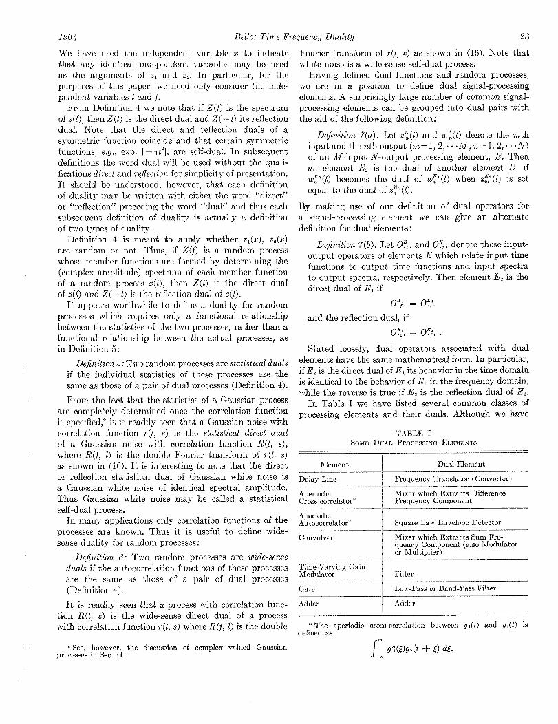
not attempted an exhaustive listing, it is worth noting that a large percentage of transmitter and receiver operations may be represented in terms of these elements. We have made a distinction between a convolver and a filter since we regard a convolver as a two-input, single- output device and a two-port filter as a single-input device. There are some types of elements not listed in Table I whose duals are not familiar and, like the aperiodic cross-correlator and autocorrelator, are not realizable as real-time operations. As an example, consider the limiter. The dual element can best be described as a spectral amplitude equalizer since the spectrum of a process in passing through this device has the magnitude of its spectrum made constant while the phase of its spectrum is unchanged. As another example, consider the linear envelope detector. Here it is clear that the dual element is best described as a spectral phase equalizer.

Definition 7(a) [and 7(b)] is meant to apply whether the elements E, and E, are random or not. In the same manner as for random processes, it is useful to define a duality for random elements which requires only a functional relationship between statistical properties of these elements rather than a functional relationship between the actual input-output operations of these elements. Thus, we provide the definition of statistical dual and wide-sense dual elements :


Fig. 3-A simple illustration of network duality.

An example of network duality is shown in Fig. 3. In the following section we give an example of system duality.

Before closing this section it should be noted that there are several obvious dual concepts such as time origin, carrier frequency and delay, doppler shift which need not be elaborated upon.

V. SOME APPLICATIONS

De&ition 8: Random element E, is the statistical dual of element E, if w,“>(t) becomes the statistical dual of w:‘(t), n = 1, 2, . a. , N, when z:“(t) is set equal to the dual of x:‘(t), m = 1, 2, . . . , M.

In this section we will present a few examples to illustrate the range of application of time-frequency duality.

A. A System Dual of the Kineplex Xystem

Definition 9: Random element E, is the wide-sense dual of E, if w:‘(t) becomes the wide-sense dual of w,“>(t), n = 1, 2, . . . , N, when .z:~ (t) is set equal to the dual of z:‘(t), m = 1, 2, . . . , JF.

The graph of a communication-signal processing network may be found by representing every element by an appropriately labeled node with directed arrows emanating to indicate inputs and outputs.

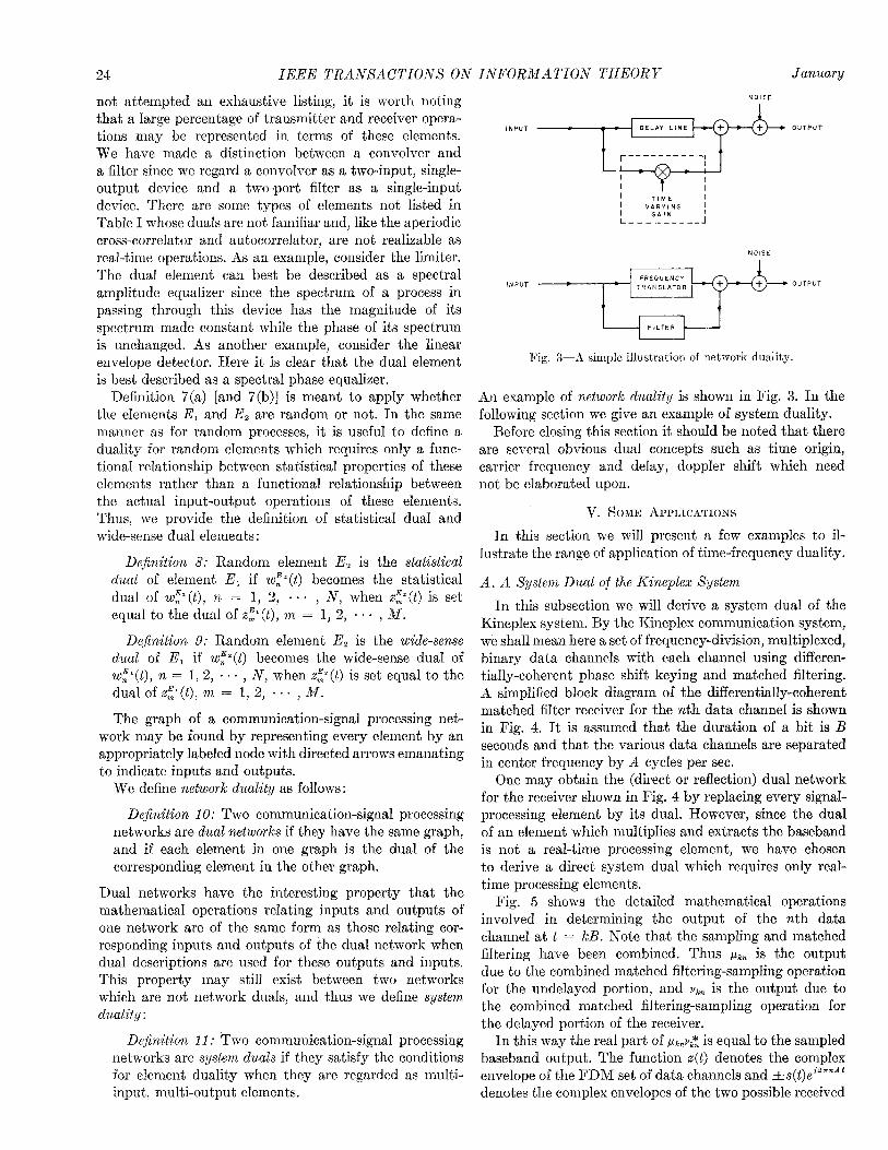
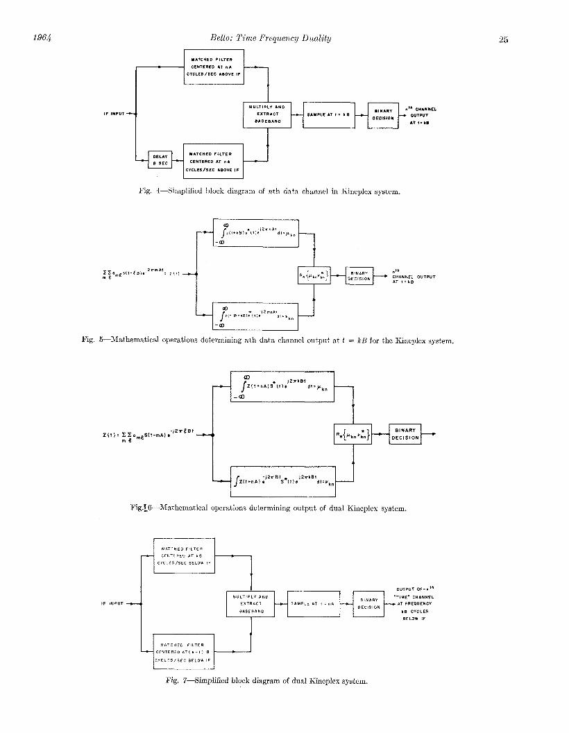
In this subsection we will derive a system dual of the Kineplex system. By the Kineplex communication system, we shall mean here a set of frequency-division, multiplexed, binary data channels with each channel using differentially-coherent phase shift keying and matched filtering. A simplified block diagram of the differentially-coherent matched filter receiver for the nth data channel is shown in Fig. 4. It is assumed that the duration of a bit is B seconds and that the various data channels are separated in center frequency by A cycles per sec.

We define network duality as follows :

DeJinition 10: Two communication-signal processing networks are dual netloorks if they have the same graph, and if each element in one graph is the dual of the corresponding element in the other graph.

Dual networks have the interesting property that the mathematical operations relating inputs and outputs of one network are of the same form as those relating corresponding inputs and outputs of the dual network when dual descriptions are used for these outputs and inputs. This property may still exist between two networks which are not network duals, and thus we define system duality :

One may obtain the (direct or reflection) dual network for the receiver shown in Fig. 4 by replacing every signal- processing element by its dual. However, since the dual of an element which multiplies and extracts the baseband is not a real-time processing element, we have chosen to derive a direct system dual which requires only real- time processing elements.

Fig. 5 shows the detailed mathematical operations involved in determining the output of the nth data channel at t = kB. Note that the sampling and matched filtering have been combined. Thus pkn is the output due to the combined matched filtering-sampling operation for the undelayed portion, and %, is the output due to the combined matched filtering-sampling operation for the delayed portion of the receiver.

Dejhition 11: Two communication-signal processing In this way the real part of I.L~,P,* is equal to the sampled networks are system duals if they satisfy the conditions baseband output. The function z(t) denotes the complex for element duality when they are regarded as multi- envelope of the FDM set of data channels and fs(t)eizrnat input, multi-output elements. denotes the complex envelopes of the two possible received

1964 Belle: l’ime Frequency Duality 25

Fig. h--Simplified block diagram of nth data channel in Kineplex system.

Fig. 5-Mathematical operations determining nth data channel output at t = kl3 for the Kineplex syst,em.

BINARY

DECISION

I I Fig.IG-Mathematical operations determining output of dual Kineplex system.

Fig. 7-Simplified block diagram of dual Kineplex system.


pulses of duration B set which may be received by the system it is not the previous baud that is used to establish nth data channel in the time interval 0 < t < B. In a phase reference but the baud occurring at the same time conventional systems the pulse s(t) would be a rectangular which is just above it in frequency. This implies that the video pulse and AB would equal an integer to remove original information must be encoded as phase-shift interchannel interference. We shall assume AB equals keying along a frequency rather than time ‘axis. These an integer but we shall leave s(t) arbitrary in the present results might have been expected a priori from the fact discussion. The complex envelope of the receiver input that the dual of a single data channel, i.e., a pulse train x(t) is given by in time confined to a frequency slot, must be a train of

z(t) = c c a,&t - ZB)ejzsmAt (27) pulses in frequency, i.e., a frequency division multiplexed

m 2 set of pulses, confined to a time slot. The Dual Kineplex system will perform better than where am2 is $1 or -1, depending upon whether the lth

bit in the mth FDM channel is one or zero. We obtain the desired direct system dual of the

Kineplex system by regarding the blocks containing integrals in Fig. 5 as hypothetical processing elements and replacing these elements by their direct duals. According to Definition 7(b), the direct dual element has a time domain behavior mathematically identical to the frequency domain behavior of the original element. By applying Parseval’s Theorem we find that the typical integral in Fig. 5 may be expressed in the frequency domain as follows:

the Kineplex system when phase stability of the medium is better along the frequency than the time axis. Thus, if the medium is essentially nonfrequency selective over the transmitted pulse bandwidth, the phase stability along the frequency axis will be excellent and the Dual Kineplex will outperform the Kineplex. On the other hand, we note that the Dual Kineplex system is somewhat wasteful of bandwidth, since the first channel used as a reference does not carry information and thus n + 1 channels are required rather than n in order to transmit n/A bits/second.

s z(t + kB).s*(t)e-iZ”“At dt = s W>e i2akBfS*(f - nA) df B. Dual of Detection and Estimation Problems

One may form the dual of an optimum (or suboptimum) detection or estimation problem by replacing processes, operations and constraints by their duals. If direct duals are used, the dual problem is mathematically identical to the original problem as expressed in the frequency domain. If reflection duals are used, the dual problem expressed in the frequency domain is mathematically identical to the original problem as expressed in the time domain. Thus, in either case, the solution of the dual problem is directly obtainable from the solution of the original problem. Or, of more importance, the solution of an estimation or detection problem may be found from the solution of the dual problem, if known.

= s Z(f + nA)X*(f)e’Z*kBf ~?f

(2% where S(f) is the spectrum of s(t), Z(f) is the spectrum of z(t),

Z(f) = C C a,,S(f - mA)e+2r*B’ (29) m 1 and use has been made of the fact that due to our previous assumption that AB is an integer, exp [j2rpAB] = 1 when p is an integer.

From (28) and the definition of element duality, it is readily seen that the receiver whose mathematical operations are shown in Fig. 6 is a direct system dual of the receiver in Fig. 5. Note that the combined matched- filtering sampling operations are self-dual. Strictly speak- ing, from the point of view of duality, the integrals shown in Fig. 6 should be multiplied by 6(t), a unit impulse at t = 0, since a definite integral is a constant and the dual of a constant a is an impulse of area a, i.e., as(t). We have chosen not to include the impulses since the actual Kineplex system does not compute constants Piw vkn as shown in Fig. 5, but rather a pulse whose amplitude is Re [&&]. Since the dual of a pulse of amplitude C is another pulse whose amplitude is propor- tional to C, we may be justified in representing the output of the Dual Kineplex system in the same way as the output of the Kineplex system ,i.e., as Re [+~clk,vk*,] rather than Re [&,,vk*J?f(t).

In Fig. 7 we have indicated a possible physical realization of the Dual Kineplex system. A comparison of Figs. 4 and 7 reveals a fundamental difference between the operation of the Kineplex and Dual Kineplex communication systems, namely, that in the Dual Kineplex

To illustrate the above ideas, consider the problem of determining the transfer function of a time-variant scatter channel through spectral analysis of the response of the channel to a very narrow pulse. It is assumed that the scatter channel consists of a large number of densely distributed scatterers, each providing different delays and Doppler-Shifts. The response of this channel to a narrow pulse of bandwidth W will be a pulse of noise of bandwidth W + 6, where 6 is the Doppler-Spread. It is assumed that the transfer function of the scatter channel is to be examined for a range of frequencies small compared with W. In this case, for all practical purposes, one may model the impulse response of the medium as a pulse of wide-sense stationary white noise. Thus, assuming the usual receiver additive white noise we observe a process

w(t) = z(t) + n(t) (30) where x(t) is a “gated” white noise with autocorrelation function5

6 In the scatter measurement problem described above, p(t) has the physical significance of the profile of scattered power vs multipath delay.

19@ Belle: Time Frequency Duality 21 ‘r

x*(t)x(s) = p(t)d(s - t), (31) where it will be recalled that p( - f) is the power spectrum

and n(t) is a wide-sense stationary white noise with of Z(t). Thus it follows that the optimum gating function

(double-sided) power density N,. The corresponding is given by

complex amplitude spectra, Z(f) and N(f), have correlation PC0

functions g(t) = p(t) + No’

(35)

Z*(f)Z(Z) = R(Z - f) (32)

It is no more difficult to obtain the answer to the optimum

N*(f)N(O = No W - f) gating function in the other more complicated cases.

where the frequency correlation function R(v) is the C. Dual of Channel Capacity Theorems

Fourier transform of the gating function p(t). %‘or every channel capacity theorem there is a dual We desire to find an optimum gating function g(t) theorem which is applicable for the case of dual channel

such that the spectrum of g(t)w(t) differs from the spectrum and signal constraints. As an illustration, consider of x(t) as little as possible in a mean-squared error sense. Shannon’s channel capacity theorem

In the direct dual problem we observe a process

w(t) = Z(t) + N(t), (33) C = W log2 [ 1 -I- &] bits/see (36)

where from (31) and (32)) it is readily seen that Z(t) where C is the capacity of a channel of bandwidth W is a wide-sense stationary noise with power spectrum perturbed by stationary white Gaussian noise of (two- p(--f), and N(t) is a wide-sense stationary white noise sided) power density N, when the average signal power with (double sided) power density N,. is limited to P.

Since the dual of gating is filtering, the direct dual In the dual case, we deal with a time-limited rather problem is one of estimating Z(t) in a minimum mean- than band-limited channel and a signal whose spectrum squared error sense by passing W(t) through a linear has an average power constraint of P’. The additive filter. This problem is recognized as the classical optimum white Guassian noise is unchanged since it is self-dua1, linear filtering problem. In the most general case, called By replacing quantities by duals in (36)) we arrive the finite observation time case,‘j the filter is constrained at the capacity of this channel as to have an impulse response of finite duration. The special case of an impulse response which vanishes for C’ = T log, [ I+ ~1 bits/cps (37) negative time is called the realizable jilter case.? In the least restrictive situation, we have the infinite Zag case’ where T is the duration of the time constraint. Note wherein the impulse response is not constrained to vanish that this capacity is measured in bits per cycle/see for negative time. rather than bits/see.

In our problem, we may distinguish three classes of The coding technique implied by (37) is a coding gating problems according to whether the gating function along the frequency rather than time axis, and C’ gives has frequency components in a finite bandwidth, has no the maximum number of bits per unit frequency that frequency components below a given frequency or has can be packed along the frequency axis and yet achieve no constraints as to the location of frequency components. error-free decoding when the signals are constrained to

For simplicity, we will illustrate the technique of the same time interval of duration T. solution for the optimum gating function only in the The number of bits transmitted in the original channel case where no constraint is placed on the location of the in T’ seconds is given by frequency components of the gating function, g(t). This corresponds to the infinite lag case in the dual problem. CT’ = WI” log,

The (direct) dual operation of gating with g(t) is 1 (38)

filtering with a filter transfer function g( -f). Thus, if where Err = PT’ is the average signal energy in a t,ime the optimum linear filter transfer function is known for interval 7”. Similarly, the number of bits transmitted the dual problem, we may immediately write down the in the dual channel in W’ cycles/see is given by solution for the optimum gating function in our problem.

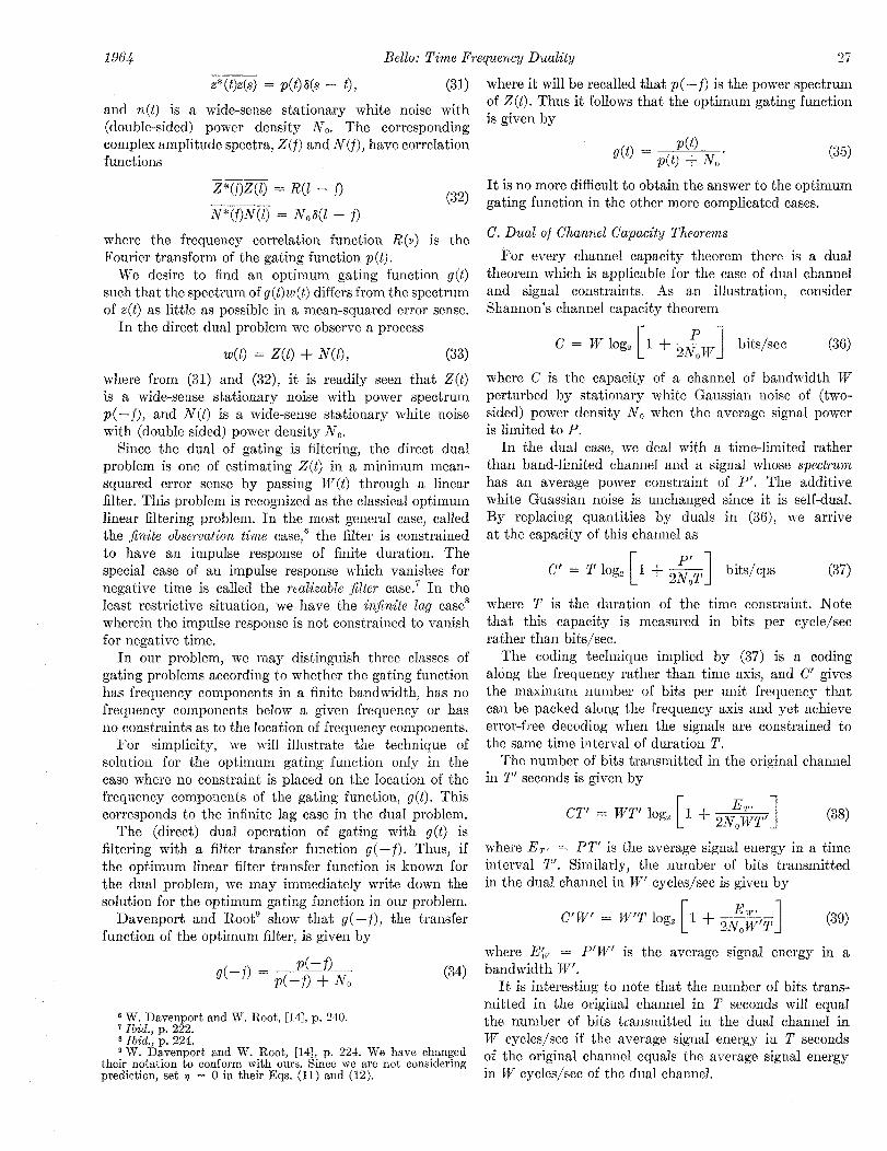
Davenport and Root’ show that g(-f), the transfer C’W’ = W’T log, function of the optimum filter, is given by 1 (39)

d-f) = PC-f) where E{, = P’W’ is the average signal energy in a

PC-~) + No (34) bandwidth W’. It is interesting to note that the number of bits trans-

mitted in the original channel in T seconds will equal 6 W. Davenport and W. Root, [14], p. 240. ’ Ibid, p. 222. the number of bits transmitted in the dual channel in 8 Ibid., p. 224. W cycles/see if the average signal energy in T seconds 9 W. Davenport and W. Root, [14],. p. 224. We have changed

their notation to conform with ours. Smce we are not considering of the original channel equals the average signal energy prediction, set v = 0 in their Eqs. (11) and (12). in W cycles/see of the dual channel.

28 IEEE TRANSACTIONS ON

D. System Functions for Time-Variant Linear Channels

The characterization of time-variant linear filters (whether random or not) in terms of system functions received its first general analytical treatment by Zadeh [15] who introduced the Time-Variant Transfer Function and the Bi-Frequency Function as frequency domain methods of characterizing time-variant linear filters to complement the time-variant impulse response which is a time domain method of characterization. Further interesting work on the characterization of time-varying linear filters in terms of system functions has been done by Kailath [12] who has pointed out that a third type of impulse response may be defined in addition to the two already used for time-variant linear filters. He has defined single and double Fourier transforms of these impulse responses in order to demonstrate that certain variables may be identified with frequencies at the filter input and output and that certain variables may be identified with the rate of variation of the filter. However, (excepting the Time-Variant Transfer Function) only the impulse responses and their double Fourier transforms were demonstrated to be system functions; i.e., filter input-output relations were derived which used only the impulse responses and their double Fourier transforms.

We demonstrate that time-varying linear channels (or filters) may be characterized in an interesting symmetrical manner in time and frequency variables by arranging system functions in (time-frequency) dual pairs. Most of these system functions (which include, among others, those introduced by Zadeh and Kailath) are shown to imply circuit model interpretations or representations of the time-varying linear channels. The relationships between these system functions will be demonstrated in a simple way with the aid of a diagram involving Duality and Fourier transformations.

1) Kernel System Functions: The starting point for our discussion is the set of equations, (26), which defines dual operators for a single-input, single-output device. In the case of a linear device such as a linear time-variant channel, the four equations in (26) may be formally” expressed as linear integral operators with associated kernels, i.e.,

w(t) = s 4dK,(t, 4 ds JW) = 1 -WKdf, 1) dl (46)

w(t) = 1 Z(fK(t, f) df W(f) = /4WL(fr t) dt. (41)

These kernels are, in effect, system functions and we shall call them kernel system functions to distinguish them from other classes of system functions to be described. It is clear that the system function pairs K,, K, and K,, K, may be considered as dual system function pairs.

The system functions I<,(& s) and K,(J, I) may be recognized as the Time-Variant In~pulse Response and the

10 In order to include linear differential operators, one must assume that the kernels may include singularity functions.


B&Frequency Function respectively, used by Zadeh [l]. The system functions Ka(t, f) and K4(f, t) have not been defined previously. Without difficulty it may be established that Kl(t, s) and K,(f, Z), besides being duals, are double Fourier transform pairs and similarly that the dual pairs K3(t, S) and K4(f, t) are double Fourier transform pairs. Also K,(t, s) and K,(t, f) are single Fourier transform pairs with t considered as a parameter while K*(f) Z) and K4(f, t) are single Fourier transform pairs with f considered as a parameter. It is worth noting that K,, K, and K,, K, are the only dual pairs of system functions among those to be presented which are related directly as double Fourier transform pairs.

The kernel system functions have simple physical interpretations in terms of the response of the channel to impulses and cissoids. Thus, it is readily determined that if the channel is excited with a unit impulse at t = s, the resulting channel output is the time function K,(t, s) with spectrum K4(f, s), while if the channel is excited with the cissoid eizrLt (i.e., frequency impulse at f = I), the resulting channel output is the time function K,(t, 1) with spectrum K,(f, I).

2) Delay-Spread and Doppler-Spread Functions: From a strictly mathematical point of view, the kernel system functions are sufficient to describe the time-frequency, input-output relations for a time-variant linear channel. From a physical-intuitive or engineering point of view, they are not as satisfactory, since they do not readily allow one to grasp by inspection the way in which the time-variant filter affects input signals to produce output signals. In the following subsections we will be concerned with system functions which, via circuit model analogies, provide a somewhat more physical interpretation of the action of the linear time-variant channel.

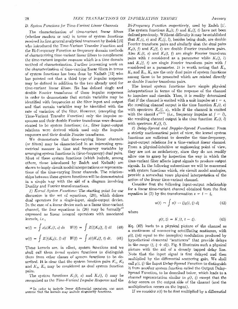
Consider first the following input-output relationship for a linear time-variant channel obtained from the first equation in (2) by the transformation s = t - .$,

40 = / 4t - Mt, 0 d$ (42)

where

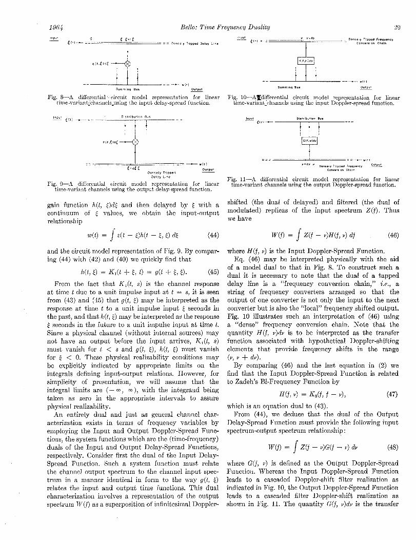
dt, 0 = Kl(t, t - 0. (43) Eq. (42) leads to a physical picture of the channel as a continuum of nonmoving scintillating scatterers, with g(t, {)dE equal to the (complex) modulation produced by hypothetical elemental “scatterers” that provide delays in the range (E, E + do. Fig. 8 illustrates such a physical picture with the aid of a densely tapped delay line. Note that the input signal is first delayed and then multiplied by the differential scattering gain. We shall call g(t, t) the Input Delay-Spread Function to distinguish it from another system function called the Output Delay- Spread Function, to be described below, which leads to a channel representation similar to g(t, 0 except that the delay occurs on the output side of the channel (and the multiplication occurs on the input).

If we consider x(t) to be first multiplied by a differential

1964 Belle: Time Frequency Duality

-- I I I -- --+--WC,) S”nlrni”Q Bur out$M

Fig. S---8 differential “circuit model representation for linear time-variantLchannelslusing the input dela.y-spread function.

Fig. 9-A differential circuit model representation for linear time-variant channels using the output delay-spread function.

gain function h(t, .$)dg and then delayed by { with a continuum of t values, we obtain the input-output relationship w(t) = s 4t - OMt - E, 0 4 (44)

and the circuit model representation of Fig. 9. By comparing (44) with (42) and (40) we quickly find that

Mt, 8 = K,(t + t, t> = dt + E, 0. (45)

From the fact that K,(t, s) is the channel response at time t due to a unit impulse input at t = s, it is seen from (43) and (45) that g(t, .$) may be interpreted as the response at time t to a unit impulse input .$ seconds in the past, and that h(t, {) may be interpreted as the response 6 seconds in the future to a unit impulse input at time t. Since a physical channel (without internal sources) may not have an output before the input arrives, K,(t, s) must vanish for t < s and g(t, 0, h(t, t) must vanish for .$ < 0. These physical realizability conditions may be explicitly indicated by appropriate limits on the integrals defining input-output relations. However, for simplicity of presentation, we will assume that the integral limits are (- ~0, a), with the integrand being taken as zero in the appropriate intervals to assure physical realizability.

An entirely dual and just as general channel characterization exists in terms of frequency variables by employing the Input and Output Doppler-Spread Func- tions, the system functions which are the (time-frequency) duals of the Input and Output Delay-Spread Functions, respectively. Consider first the dual of the Input Delay- Spread Function. Such a system function must relate the channel output spectrum to the channel input spectrum in a manner identical in form to the way g(t, t) relates the input and output time functions. This dual characterization involves a representation of the output spectrum W(f) as a superposition of infinitesimal Doppler-

\:(_i -v,,l

summng 8”s O”Ip”f

ial circuit model representation for linear els using the input Doppler-spread function.

Fig. lb--rl differential circuit model representation for linear time-variant channels using the output Doppler-spread function.

shifted (the dual of delayed) and filtered (the dual of modulated) replicas of the input spectrum Z(f). Thus we have

W(f) = / z(f - vW(f, v> df (46)

where H(f, V) is the Input Doppler-Spread Function. Eq. (46) may be interpreted physically with the aid

of a model dual to that in Fig. 8. To construct such a dual it is necessary to note that the dual of a tapped delay line is a “frequency conversion chain,” i.e., a string of frequency converters arranged so that the output of one converter is not only the input to the next converter but is also the Yocal” frequency shifted output. Fig. 10 illustrates such an interpretation of (46) using a “dense” frequency conversion chain. Note that the quantity H(f, v)dv is to be interpreted as the transfer function associated with hypothetical Doppler-shifting elements that provide frequency shifts in the range (v, v + dv).

By comparing (46) and the last equation in (2) we find that the Input Doppler-Spread Function is related to Zadeh’s Bi-Frequency Function by

Wf, v> = Uf, f - ~1, (47)

which is an equation dual to (43). From (44), we deduce that the dual of the Output

Delay-Spread Function must provide the following input spectrum-output spectrum relationship :

W(f) = j z(f - vMf - v> dv (48)

where G(f, v) is defined as the Output DoppIer-Spread Function. Whereas the Input Doppler-Spread Function leads to a cascaded Doppler-shift filter realization as indicated in Fig. 10, the Output Doppler-Spread Function leads to a cascaded filter Doppler-shift realization as shown in Fig. 11. The quantity G(f, v)dv is the transfer


function of a hypothetical differential filter at the input which is associated with a Doppler shift of v cycles/see at the channel output.

By comparing (48) with (47) and (40) we find that

G(f, v> = Kdf + ~7 f) = H(f + ~9 v>, (49)

which is a set of equations dual to (45). Since K,(f, 1) is the value of the spectral response of the channel at a frequency f due to a cissoidal excitation of frequency 1 cycles/set, it is quickly seen from (47) and (49) that H(f, v) may be interpreted as the spectral response of the channel at f cycles/see due to a cissoidal input which is v cycles below f, and that G(f, V) may be interpreted as the spectral response of the channel at a frequency v cycles/see above the cissoidal input at the frequency f cycles/set.

S) Time-Variant Transfer Function and Frequency- Dependent Modulation Function: The characterizations of a time-variant channel, in terms of the Delay Spread Functions g(t, l) and h(t, E), and the time-variant impulse response K,(t, s) are strictly time domain approaches while the characterizations in terms of the Doppler Spread Functions H(f, v) and G(f, v) and the Bifrequency Function K2(f, 1) are entirely frequency domain approaches. In the former cases the output time function is directly related to the input time function, while in the latter cases the output spectrum is directly related to the input spectrum. As discussed in Section V-D, 1) and exemplified by the dual kernel system functions K3(t, f) and K4(f, t), two other approaches are possible. These involve an expression of the output time function directly in terms of the input spectrum in one case and an expression of the output spectrum directly in terms of the input time function in the other case. An example of the former approach was first introduced by Zadeh [15] with the aid of the Time-Variant Transfer Function.

In this subsection we will introduce a new system function called the Frequency-Dependent Modulation Function which is the (time-frequency) dual of the Time- Variant Transfer Function. This system function relates the output spectrum to the input time function.

Assuming we have an input, x(t), which may be represented as a summation of infinitesimal cissoidal time functions, i.e.,

x(t) = 1 Z(f)ei2”‘t df (50)

where Z(f) is the spectrum of x(t), one may determine the channel output by superposing the separate responses to the infinitesimal cissoidal components. The response of the channel to the cissoidal time function exp [j2&] (or spectral impulse S(f - 1)) is given [see (42)] by

s e i2r-t)g(t, [) d; = ei2TztT(Z, t) (51)

where

T(f, t) = / eeizr”g(t, .$) d.$ (52)

is the Fourier transform of the Input Delay-Spread Function with respect to the delay parameter. By superposition the network output is given by

w(t) = s Z(f)T(f, t)eiaaft df. (53)

Eq. (43) shows that even though the channel may be time-variant, one may determine the output by exactly the same frequency domain techniques as for time- invariant (linear) channels. This involves, basically, a multiplication of the input spectrum by a system function followed by an inverse Fourier transformation with respect to the frequency variable. For time-variant channels, however, the system function is a function of the time variable. This explains use of the term Time- Variant Transfer Function to denote T(f, t).

By using (48) to determine the spectrum of the response to the frequency impulse S(f - Z) and then inverse Fourier transforming to obtain the corresponding time response, it may be quickly determined that

T(f, t) = / G(f, ~)ej~=‘~ dv,

i.e., that the Time-Variant Transfer Function is the inverse Fourier transform of the Output Doppler Spread Function with respect to the Doppler-shift variable.

Also, either by noting that K3(t, Z) may be interpreted as the channel response at time t to an excitation eizuzt, as discussed in Section V-D, l), or by comparing (41) and (53), it is readily seen that

K3(t, f) = eizn’rT(f, t). (55)

To develop the dual system function, we assume that we have an input whose spectrum Z(f) may be represented as a summation of infinitesimal cissoidal frequency functions, i.e.,

Z(f) = 1 x(t)e-i2”‘t dt. (56)

The spectrum of the response of the channel to the cissoidal frequency function exp [-j27rfs] (i.e., to the time function 6(t - s) whose spectrum is exp I--jarfs]) is given [see (46)] by

s e --i-f+H(f, v) & = e-i2+M(s, f) (57)

where

M(t, f) = / eizrt”H(f, v) dv (58)


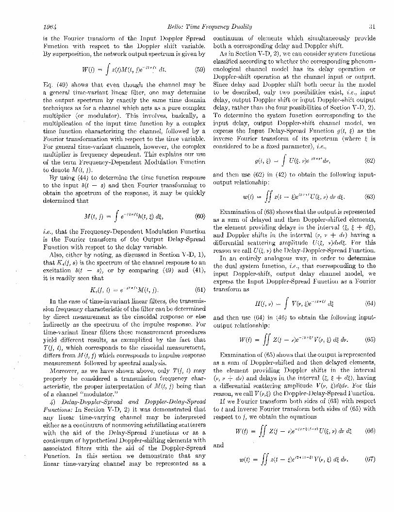
is the Fourier transform of the Input Doppler Spread Function with respect to the Doppler shift variable. By superposition, the network output spectrum is given by

W(f) = / x(t)M(t, f)evizrft dt. (59)

Eq. (49) shows that even though the channel may be a general time-variant linear filter, one may determine the output spectrum by exactly the same time domain techniques as for a channel which acts as a pure complex multiplier (or modulator). This involves, basically, a multiplication of the input time function by a complex time function characterizing the channel, followed by a Fourier transformation with respect to the time variable. For general time-variant channels, however, the complex multiplier is frequency dependent. This explains our use of the term Frequency-Dependent Modulation Function to denote M(t, f).

By using (44) to determine the time function response to the input 6(t - s) and then Fourier transforming to obtain the spectrum of the response, it may be quickly determined that

M(t, f) = / e-i2T’Eh(t, l) dt, (60)

i.e., that the Frequency-Dependent Modulation Function is the Fourier transform of the Output Delay-Spread Function with respect to the delay variable.

Also, either by noting, as discussed in Section V-D, l), that K4(f, s) is the spectrum of the channel response to an excitation 6(t - s), or by comparing (49) and (41), it is readily seen that

K,(f, t) = e-i27ftM(t, f). (61)

In the case of time-invariant linear filters, the transmission frequency characteristic of the filter can be determined by direct measurement as the cissoidal response or else indirectly as the spectrum of the impulse response. For time-variant linear filters these measurement procedures yield different results, as exemplified by the fact that T(f, t), which corresponds to the cissoidal measurement, differs from M(t, f) which corresponds to impulse response measurement followed by spectral analysis.

Moreover, as we have shown above, only T(f, t) may properly be considered a transmission frequency characteristic, the proper interpretation of ilf(t, f) being that of a channel LLmodulator.”

4) Delay-Doppler-Spread and Doppler-Delay-Spread Functions: In Section V-D, 2) it was demonstrated that any linear time-varying channel may be interpreted either as a continuum of nonmoving scintillating scatterers with the aid of the Delay-Spread l?unctions or as a continuum of hypothetical Doppler-shifting elements with associated filters with the aid of the Doppler-Spread Function. In this section we demonstrate that any linear time-varying channel may be represented as a

continuum of elements which simultaneously provide both a corresponding delay and Doppler shift.

As in Section V-D, 2), we can consider system functions classified according to whether the corresponding phenom- enological channel model has its delay operation or Doppler-shift operation at the channel input or output. Since delay and Doppler shift both occur in the model to be described, only two possibilities exist, i.e., input delay, output Doppler shift or input Doppler-shift output delay, rather than the four possibilities of Section V-D, 2). To determine the system function corresponding to the input delay, output Doppler-shift channel model, we express the Input Delay-Spread Function g(t, t) as the inverse Fourier transform of its spectrum (where .$ is considered to be a fixed parameter), i.e.,

g(t, i,) = / U(t, v)e iz”vtdv, (62)

and then use (62) in (42) to obtain the following input- output relationship :

w(t) = j”j x(t - ,$)eizavtU(E, v) dv dt. (63)

Examination of (63) shows that the output is represented as a sum of delayed and then Doppler-shifted elements, the element providing delays in the interval (<, 5 + dl), and Doppler shifts in the interval (v, v + dv) having a differential scattering amplitude U(<, v)dvd[. For this reason we call U([, v) the Delay-Doppler-Spread Function.

In an entirely analogous way, in order to determine the dual system function, i.e., that corresponding to the input Doppler-shift, output delay channel model, we express the Input Doppler-Spread Function as a Fourier transform as

H(f, v) = / V(v, .$)e-i2”E’ d.$ (64)

and then use (64) in (46) to obtain the following input- output relationship:

W(f) = I/ Z(f - v)e-‘2n’fV(v, E) dt dv. (65)

Examination of (65) shows that the output is represented as a sum of Doppler-shifted and then delayed elements, the element providing Doppler shifts in the interval (v, v + dv) and delays in the interval (& { + do, having a differential scattering amplitude V(V, Qdtdv. For this reason, we call V(v,l) the Doppler-Delay-Spread Function.

If we Fourier transform both sides of (63) with respect to t and inverse Fourier transform both sides of (65) with respect to f, we obtain the equations

W(f) = /“I Z(f - v)e-i2rf(f-“)U(E, v) dv d.$ (66)

and w(t) = ss x(t - t)e’2”‘t-e’ V(v, ij) d( dv. (67)

32 llclGJ3 ‘I’KHlVSAL’~‘l UlVb Ul\’

A comparison of (65) and (66) or (63) and (67) reveals that U({, V) and V(V, {) are simply related, i.e.,

U(.$, v) = e-j2*“V(v, {). w

If the integration with respect to [ is carried out in (66) and the integration with respect to v is carried out in (67), one finds that

h(t, l) = / V(V, <)e-jzaut dv (69)

and Fig. 12-Relationships between system functions for time-variant

linear channels. G(f, V) = 1 U(E, v)eCizrtf dt. (70)

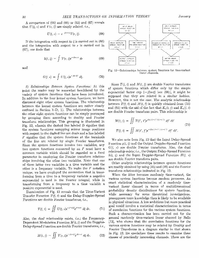
5) Relationships Between System Functions: At this point the reader may be somewhat bewildered by the variety of system functions that have been introduced. In addition to the four kernel system functions, we have discussed eight other system functions. The relationship between the kernel system functions are rather clearly outlined in Section V-D, 1). The relationships between the other eight system functions can be simply portrayed by grouping them according to duality and Fourier transform relationships. This grouping is illustrated in Fig. 12, wherein the dashed line labeled D signifies that the system functions occupying mirror image positions with respect to the dashed line are duals and a line labeled F signifies that the system functions at the terminals of the line are related by single Fourier transforms. Since the system functions involve two variables, any two system functions connected by an F must have a common variable which should be regarded as a fixed parameter in employing the Fourier transform relationships involving the other two variables. Note that one of these latter two variables is a time variable and the other is a frequency variable. To make the F notation unique, we have employed the convention that in transforming from a time to a frequency variable a negative exponential is used in the Fourier integral, while in transforming from a frequency to a time variable a positive exponential is used.

Examination of Fig. 12 reveals that the Time-Variant Transfer Function T(f, t) and the Delay-Doppler-Spread Functions are double Fourier transforms, i.e.,

T(f, t) = 11 U(g, v)e-‘nrE’ejzTvt dt dv. (71)

Also, the dual relationship exists, i.e.; the Frequency- Dependent Modulation Function fW(t, f) and the Doppler- Delay-Spread Function are double Fourier transforms, i.e.,

M(t, f) = // V(v, {)e-i2a’fei2rrt d[ dv. (72)

Since T(f, t) and M(t, f) are double Fourier transforms of system functions which differ only by the simple exponential factor exp [-j2rrvE] [see (68)], it might be supposed that they are related in a similar fashion. However, this is not the case. The analytic relationship between T(f, t) and M(t, f) is quickly obtained from (55) and (61) with the aid of the fact that K3(tj f) and K4(f, t) are double Fourier transform pairs. This relationship is

&‘(t, f) = I/” T(f’, t’)eiz=(‘-f’)(‘-t’) df’ dt’ (73)

T(f, t) = j/ &f(t’, f’)e-i2a(f-f’)(t-t’) df’ dt’.

We also note from Fig. 12 that the Input Delay-Spread Function g(t, <) and the Output Doppler-Spread Function G(f, V) are double Fourier transforms. Also, the dual relationship exists; i.e., the Output Delay-Spread Function h(t, 0 and the Input Doppler-Spread Function H(f, v) are double Fourier transform pairs.

Other analytic relationships between system functions are readily obtained by using (45) and (49) and the Fourier transform relationships indicated in Fig. 12.

When the filter becomes randomly time-variant, the various system functions become random processes. An exact statistical characterization of a randomly time- variant linear channel in terms of multidimensional probability density distributions for system functions, while necessary for some theoretical investigations, presupposes more knowledge than is likely to be available in physical situations. A less ambitious but more practical goal would involve a statistical characterization in terms of correlation functions for the various system functions. Such a characterization has been carried out for the general randomly time-variant linear channel by Bello [13], who shows that the correlation functions for the various system functions may be related by Duality and Fourier Transforms in a diagram similar to that shown in Fig. 12. He specializes these results to examine three classes of practically interesting channels. These are the

1964 Belle: Time Frequency Duality ss

wide-sense stationary (abbreviated WSS) channel, the uncorrelated scattering (US) channel, and the wide-sense [II stationary uncorrelated scattering (WSSUS) channel. PI The WSS channel is one in which g(t, {) is a wide-sense stationary process in the variable t so that the differential [31 tap gain g(t, {)dt in Fig. 8 is a wide-sense stationary process. The US channel is one in which the tap gain [41 fluctuations for different delays are uncorrelated. It is demonstrated that the WSS and US classes of channels 151

bear an interesting dual relationship : The wide-sense dual of a US channel is a WSS channel and vice versa. A El

particularly simple class of channels, the WSSUS class, arises as the intersection of the WSS and US classes.

LTl

Because of the dual relationship between the WSS and PI US classes of channels, the WSSUS class of channels -^. may properly be called a wide-sense self-dual class. Previous discussions of channel correlation functions [ 161, [17] and their relationships have dealt exclusively with the WSSUS channel.

All real-life channels and signals have an essentially finite number of degrees of freedom due to restrictions on time duration and bandwidth. This fact has been exploited by Kailath [12] to derive canonical channel models for the cases in which the channel band-limits signals at its input or output and in which the channel impulse response is time-limited. With the aid of the dual system functions, Bello [13] has derived new canonic sampling models, some of which may be identified as dual to those of Kailath. As might be expected, these dual models are particularly useful under the dual time- frequency constraints, i.e., when the input or output time functions are time-limited or when the channel fading is band-limited.

DOI

[Ill

WI

D31

r141

u51

D61

o71

D81

REFERENCES P. M. Woodward, “Probabilit,y and Information Theory,” McGraw-Hill Book Co., Inc., New York, N. Y.; 1953. J. Dugundji, “Envelopes and pre-envelopes of real waveform,” IRE TRANS. ON INFORMATION THEORY, vol. IT-4, PIX 53-57; -- March, 1958. R. Arens, “Complex processes for envelopes of normal noise,” IRE TRANS. ON INFORMATION THEORY, vol. IT-3, pp. 204-207; September, 1957. D. Gabor, “Theory of Communications,” J. IEE, pt. III, vol. 93, pp. 429-457; 1946. M. Loeve, “Second Order Properties,” in “Probability Theory,” D. Van Nostrand Co., Inc., New York, N. Y., ch. 10, sec. 34.4, 1955. A. Blanc-Lapierre and R. Fortet, “Analyse Harmonique Des Fonctions Alkatoires; Filtres Lineaires,” in “Theorie des Fonc- tions Aleatoires,” Masson, Paris, France, ch. 8; 1953. J. L. Doob, “Stochast,ic Processes,” John Wiley and Sons, Inc., New York, N. Y., ch. 11, sec. 4; 1953. H. W. Bode and C. E. Shannon, “A Simplified derivation of linear least-squares smoot,hing and prediction theory,” PROC. IRE, vol. 38, pp. 417-425; April, 1950. L. A. Zadeh and J. R. Ragazzini, “An extension of Wiener’s theory of prediction,” J. Appl. Phys., vol. 21, pp. 645-655; July, 1950. L. A. Zadeh, “Time-varying Network, I,” Proc. IRE, vol. 49, pp. 1488-1502; October, 1961. T. Kailath, “Solution of an integral equation occurring in multipath communication problems,” IRE TRANS. ON IN- FORMATION THEORY (Correspondence), vol. IT-6, p. 412; June, 1960. T. Kailath, “Sampling Models for Linear Time-Variant Filters,” M. I. T. Res. Lab. of Electronics, Cambridge, Rept. No. 352; May 25, 1959. P. Bello, “Characterization of randomly time-variant linear channels,” IRE TRANS. ON CO~MMUNICATION SYSTERIS, vol. CS-11, December, 1963. W. Davenport and W. Root, “Random Signals and Noise,” McGraw-Hill Book Co., Inc., New York, N. Y.; 1958. L. A. Zadeh, “Frequency analysis of variable networks, PROC. IRE, vol. 38, pp. 291-299; March, 1950. T. Hagfors, “Some properties of radio waves reflected from the moon and their relation to the lunar surface,” J. Geophys. Res., vol. 66, p. 777; March, 1961. P. E. Green! Jr., “Radar Astronomy Measurement Techniques,” M. I. T. Lmcoln Lab., Lexington, Tech. Rept. No. 282; De- cember, 1962. P. Bello, “On the approach of a filtered pulse train to a narrow- band Gaussian process,” IRE TRANS. ON INFORMATION THEORY, vol. IT-7, pp 144-150; July, 1961.

bellotime frequency duality

Documents