behavioral biases and the representative agent

Theory Dec. (2012) 73:97–123DOI 10.1007/s11238-011-9274-3

Behavioral biases and the representative agent

Elyès Jouini · Clotilde Napp

Published online: 15 July 2011© Springer Science+Business Media, LLC. 2011

Abstract In this article, we show that behavioral features can be obtained at a grouplevel even if they do not appear at the individual level. Starting from a standard modelof Pareto optimal allocations, with expected utility maximizers but allowing for heter-ogeneity among individual beliefs, we show in particular that the representative agenthas an inverse S-shaped probability distortion function as in Cumulative prospecttheory.

Keywords Behavioral biases · Probability weighting function ·Representative agent

JEL Classification G11 · D81 · D84 · D87 · D03

1 Introduction

In this article, we analyze a model of Pareto optimal allocations with von Neuman Mor-genstern utility maximizing agents. Agents are heterogeneous, in the sense that they

Electronic supplementary material The online version of this article(doi:10.1007/s11238-011-9274-3) contains supplementary material, which is available to authorized users.

E. Jouini (B)CEREMADE, Université Paris Dauphine, Place du Maréchal de Lattre de Tassigny,75 775 Paris cedex 16, Francee-mail: [email protected]

C. NappCRNRS-DRM and Université Paris Dauphine, Place du Maréchal de Lattre de Tassigny,75 775 Paris cedex 16, Francee-mail: [email protected]

123

http://dx.doi.org/10.1007/s11238-011-9274-3

98 E. Jouini, C. Napp

might differ in their beliefs. At the aggregate level, the social welfare function of thiseconomy is characterized by a social/representative belief. We show that we retrieve,at the aggregate level, behavioral properties even though they are not assumed at theindividual level. The group acts as a behavioral agent and this behavioral property atthe aggregate level is generated by heterogeneity alone.

We start by introducing natural notions of optimism and pessimism and we assumethat beliefs are heterogeneous enough in order to allow for optimistic as well as pessi-mistic agents in the initial set of von Neuman Morgenstern utility maximizing agents.In such a setting, we obtain that the representative agent1 can neither be everywhereoptimistic nor everywhere pessimistic; she is optimistic for the good states of theworld and pessimistic for the bad states of the world. As in the SP/A Theory of Lopes(1987), the representative agent behaves as if she had fear (need for security) for verybad events and hope (desire for potential) for very good events. The representativeagent puts more weight on extreme events. We show that the distribution of outcomesfrom the representative agent point of view is portfolio dominated by the objectivedistribution. This means that heterogeneity generates doubt at the aggregate level.This effect is reinforced when agents are more risk tolerant or when there is moreheterogeneity among agents.

The representative agent distorts the objective distribution of aggregate endow-ment. We analyze this distortion and we show that the distortion function (defined asthe transformation of the objective decumulative distribution function into the decu-mulative distribution function of the representative agent) is inverse S-shaped as is theprobability weighting function in Cumulative prospect theory. We show that we areable to fit relatively well standard probability weighting functions of the CPT literature(Tversky and Kahneman 1992; Tversky and Fox 1995; Prelec 1998, among others).According to Gonzalez and Wu (1999) terminology, attractiveness at the aggregatelevel is directly related to the average level of optimism while discriminability isrelated to beliefs heterogeneity.

The idea that an inverse S-shaped probability weighting function may be the resultof aggregation has been put forward by Luce (1996). However, in this last reference,the aggregation is of statistical nature (the author considers an average of differentsubjects) while our aggregation is in terms of representative agent.

Note that we don’t pretend to retrieve all features of CPT on the aggregate belief.We only retrieve one of the three main features of CPT, namely the inverse S-shapedprobability distribution weighting function (the other two being the presence of a ref-erence point and of loss aversion). We have introduced heterogeneity on the beliefsonly and it is then natural to retrieve behavioral properties that deal with beliefs only.

The article is organized as follows: Sect. 2 presents the model. Section 3 analysesthe properties of the belief of the representative agent. Section 4 proposes extensionsand remarks. All proofs can be found in the electronic web appendix.2

1 See Jouini and Napp (2007) for the existence and the construction of such a representative agent.2 http://www.ceremade.dauphine.fr/~jouini/.

123

http://www.ceremade.dauphine.fr/~jouini/

Behavioral biases and the representative agent 99

2 The setting

We consider an economy with a single consumption good and with agents who havethe same utility function but heterogeneous beliefs. Aggregate endowment in the con-sumption good is described by a random variable e∗ defined on a probability space(�, F, P) . We let I denote the set of heterogeneous agents.3 We assume that the

common utility function is CRRA with derivative given by u′(x) = x− 1η . Each agent

has a subjective belief Qi and wants to maximize her von Neumann Morgenstern util-ity for consumption of the form Ui (c) = E Qi [u (c)] . We let Mi denote the densityof Qi with respect to the probability P , hence agent i’s utility for consumption canequivalently be written in the form Ui (c) = E

[Mi u (c)

].

In such an economy, we consider the aggregate utility function U defined as thesolution of the following maximization program

U (e∗) ≡ max∑i∈I yi =e∗

∑

i∈I

λi E[

Mi u(yi )]

where (λi ) are given positive weights. The aggregate utility function corresponds tothe value of the social welfare function at the Pareto optimum when agent i is granteda weight λi by a social planner. The index i may also represent a group of agents withcommon beliefs Mi ; yi then represents the total consumption of the group and λi thesum of the weights granted by the social planner to the individuals in the group. Whenthe social planner grants the same weight to all the agents in the economy, the weightλi represents the proportion of agents that have the same belief Mi . From a socialplanner point of view, the aggregate utility function corresponds to the highest socialutility level among all possible endowment distributions across agents.

The function U can represent the utility of a group I of agents (household, villagecommunity) assuming that each member of the group has specific beliefs Qi and thatthe group behavior results from a bargaining process leading to a Pareto efficient allo-cation of resources (yi ). The bargaining process attaches a weight λi to each memberof the group; these weights can then be interpreted as bargaining power. This is forinstance the approach adopted in the collective model of the household developed byChiappori (1988, 1992).4 This approach is to be contrasted with non cooperative orstrategic approaches, as in, e.g., Ulf (1988), which rely on Cournot-Nash equilibria.

We obtain the following representation result.

Proposition 1 Representative Agent

The aggregate utility for consumption is given by

U (e∗) = E[Mu(e∗)

]

3 The number of agents can be finite or infinite. In the case of an infinite number of agents, sums arereplaced by integrals.4 See also Abdellaoui et al. (2010) where the groups under consideration are couples, as well as Mazzoccoand Saini (2011) and Chiappori et al. (2010) where the groups under consideration are village communities.

123


with

M =(

∑

i∈I

γi

(Mi

)η) 1

η

(1)

for γi = ληi . The representative agent belief is then given by M = (∑

i∈I γi(Mi

)η) 1η .

This means that, at the Pareto optimum, the aggregate utility is given by the utilityof a representative agent endowed with an average belief (and the same utility functionas each of the agents). In particular, if all the agents share the same belief, then therepresentative agent will share this common belief. If we think of e∗ as a given pros-pect for the group I of agents, the aggregate utility U (e∗) corresponds to the socialwelfare associated with the optimal allocation of e∗ across the members of the groupand is given by the utility of the representative agent.

In the case where the distribution of e∗ for agent i admits a density5 (for all i ∈ I )denoted by f i and where the distribution of e∗ under the probability P also admitsa density denoted by f , the following Corollary characterizes the density of e∗ forthe representative agent. Since we don’t have E [M] = 1 (except in the specific log-arithmic utility setting) we need first the following technical definition. We say thatthe distribution of a random variable X admits a “density fX for the representativeagent” if for all function h, we have E [Mh (X)] = ∫

h (x) fX (x) dx . Moreover, inorder to analyse the relative weights of the different states of the world from the rep-resentative agent point of view, we introduce the probability measure Q defined bydQdP ≡ M

E[M] .

Corollary 2 The distribution of e∗ admits the following density for the representativeagent

f M =(

∑

i∈I

γi

(f i

)η)1/η

which is a power average of the initial densities. In particular, for η = 1, the dis-tribution of e∗ for the representative agent is a mixture of the individual subjectivedistributions.

As an immediate consequence of Corollary 2, we get that for any measur-able real-valued function ϕ, the distribution of ϕ (e∗) admits the density f M,ϕ =(∑

i∈I γi(

f i,ϕ)η)1/η

for the representative agent where f i,ϕ denotes the density ofthe distribution of ϕ (e∗) for agent i. This implies in particular that in the case η = 1,

if each agent anticipates a normal distribution on log e∗, then the distribution of log e∗is a mixture of normal distributions for the representative agent.

5 In other words, the distribution of e∗ under Qi is absolutely continuous with respect to the Lebesguemeasure.

123


3 Behavioral properties of the group

In this Section, the aggregate endowment e∗ as well as the individual beliefs Mi areconsidered as given and we analyze the distributional properties of e∗ from the grouppoint of view. In particular, we show that this agent distorts the distribution of e∗ aswould a CPT agent. At this stage, our representative agent is an expected (subjective)utility maximizer as can be seen through Proposition 1. In Sect. 4 we will see that moresophisticated constructions lead to agents who distort the distribution of any prospectas would a CPT agent.

3.1 Illustrative examples

The next two simple examples illustrate some qualitative properties of the endowmentdistribution from the representative agent point of view. The proofs can be found inthe web appendix.

Example 1 Let us assume that all utility functions are logarithmic (η = 1). We have

E Q [e∗] =

∑

i∈I

γi E Qi[e∗] ,

which means that the mean at the aggregate level is given by an arithmetic average ofthe individual means. The variance is given by

VarQ [e∗] =

∑

i∈I

γi VarQi[e∗] + Vari

(E Qi

[e∗]) ,

where Vari

(E Qi

[e∗]) ≡ ∑

i∈I γi(E Qi

[e∗])2 − (∑

i∈I γi E Qi[e∗])2

measuresbeliefs (on the mean) heterogeneity. This means that the variance at the aggregatelevel is given not only by an arithmetic average of the individual variances, but alsoby an additional term related to beliefs dispersion. The variance is “increased” at theaggregate level and this increase is proportional to the level of beliefs heterogeneity:beliefs heterogeneity generates “doubt”.

Example 2 Let us assume that the objective distribution of aggregate endowment islognormal with e∗ ∼P ln N (μ, σ 2) and that we have two equally weighted groups ofagents, both with lognormal subjective distributions for aggregate endowment, e∗ ∼Qi

ln N (μi , σ2) for i = 1, 2. The distribution of log e∗ for the representative agent is not

Gaussian and when agents’ beliefs are heterogeneous enough (|μ1 − μ2| > 2σ√η

), the

distribution of log e∗ is bimodal (see Fig. 1). When μ = μ1+μ22 , the distribution of

log e∗ for the representative agent is Portfolio dominated6 by the objective distribu-tion. Hence, aggregate endowment e∗ is considered as more risky by the representative

6 Let us recall that a distribution f dominates a distribution g in the sense of Portfolio dominance ( f �P Dg) if we have

∫u′(x)(x − a) f (x)dx = 0 ⇒ ∫

u′(x)(x − a)g(x)dx ≤ 0 for any real number a and anynon-decreasing concave function u. This concept has been introduced in the context of portfolio problems

123


Fig. 1 In this figure, we have represented in black the consensus belief in a log-utility agents setting.A proportion of 47% of the agents believe that log e ∼ N (0, 1) and the remaining 53% believe thatlog e ∼ N (2.5, 1). The beliefs of these two categories of agents are represented in gray

Fig. 2 In this figure we represent the consensus belief for three different levels of risk aversion. We assumethat a proportion of 47% of the agents believe that log e ∼ N (0, 1) and the remaining 53% believe thatlog e ∼ N (2.5, 1). The upper curve corresponds to η = 2, the lower curve to η = 0.8 and the middle curveto η = 1. An increase of η increases the distance between the peaks and their size

agent than it actually is. In particular, we have VarQ[log e∗] > VarP

[log e∗]. This

last property still holds for general (μi ). Figures 1 and 2 illustrate these conclusionsin different settings. Note that Fig. 1 is similar to Figure 8.2 in Shefrin (2005). Forη > η′ and associated representative agent probability measures Qη and Qη′

, wehave dQη

dQη′ = hη,η′(e∗) where hη,η′ is symmetric with respect to μ1+μ22 , decreasing

before μ1+μ22 and increasing after μ1+μ2

2 . A higher level of risk tolerance induces

Footnote 6 continuedby Landsberger and Meilijson (1993) and further studied by Gollier (1997). It characterizes the changesin the distribution of the returns of the risky asset that lead to an increase in demand for the risky assetirrespective of the risk-free rate. It is then related to the degree of riskiness. See also Jouini and Napp (2008).

123


then a portfolio dominated shift in the representative agent’s distribution. In particu-lar, VarQ

[log e∗] increases with the level or risk tolerance η. The interpretation is the

following. When there is heterogeneity, each agent consumes a larger proportion ofaggregate endowment in states of the world that she considers more likely. This leadsto heterogeneous allocations and generates variance at the aggregate level. However,this effect is counterbalanced by risk aversion. Consequently, the higher the level ofrisk tolerance, the more heterogeneous the members of the group are in their optimalallocations. Figure 2 illustrates this result.

3.2 Qualitative properties

This section deals with notions of optimism and pessimism at the individual as wellas at the representative agent level. For normal distributions N (μi , σ

2), there is anatural order on the set of possible densities induced by the natural order on the means(μi ). Agents with a larger (resp. smaller) μi can be referred to as more optimistic(resp. pessimistic). For general distributions (with densities), we define relative pessi-mism/optimism in the following way. If we assume that P is the objective probability,then we are also able to introduce absolute notions of pessimism/optimism.

Definition 1 For i, j ∈ I, agent i is said to be more optimistic than agent j and wedenote it by fi �opt f j if and only if fi

f jis nondecreasing. The optimism relation �opt

is an order on the set ( fi )i∈I . If P is the objective probability, then agent i is said tobe optimistic (resp. pessimistic) if fi

f is nondecreasing (resp. nonincreasing).

Definition 1 can be rephrased in terms of Monotone likelihood ratio dominance(MLR)7: agent i is more optimistic than agent j if the distribution of e∗ for agent i(i.e., under Qi ) dominates the distribution of e∗ for agent j (i.e., under Q j ) in thesense of the MLR. For a given agent i, if we let gi denote the transformation of theobjective decumulative distribution function F into the agent’s subjective decumu-lative distribution function Fi , i.e., such that Fi = gi ◦ F, it is easy to check thatfif is nondecreasing (resp. nonincreasing) if and only if gi is convex (resp. concave).

This means that our concept of optimism/pessimism is the analog, in the expectedutility framework, of the concept of optimism/pessimism introduced by Diecidue andWakker (2001) in a RDEU framework. Other concepts of optimism/pessimism havebeen proposed in the literature. In particular, Yaari (1987), Chateauneuf and Cohen(1994), and Abel (2002) propose a definition based on First stochastic dominance.8

Note that MLR dominance is stronger than FSD.A MLR dominated shift for a given distribution reduces the mean and if fi �opt f j

then we have E Qi[e∗] ≥ E Q j

[e∗]. This last condition characterizes the MLR dom-

7 This concept is widely used in the statistical literature and was first introduced in the context of portfolioproblems by Landsberger and Meilijson (1990). More precisely, Landsberger and Meilijson (1990) showedthat in the standard portfolio problem a MLR shift in the distribution of returns of the risky asset leads toan increase in demand for the risky asset for all agents with nondecreasing utilities.8 More precisely, in an expected utility framework Abel (2002) defines pessimism by the condition Fi ≥ F(First Stochastic Dominance) that corresponds to the condition gi ≥ I d introduced by Chateauneuf andCohen (1994) in a RDEU setting.

123


inance when we restrict our attention to a family of lognormal distributions with thesame variance parameter and we then retrieve that agent i is more optimistic thanagent j if and only if μi > μ j . In that case, optimistic (resp. pessimistic) agents arethen characterized by μi > μ (resp. μi < μ) as in Shefrin (2005).

Proposition 3 We suppose that there are at least one optimistic agent denoted by fopt

and one pessimistic agent denoted by fpess in the set I of agents. We also assume that

lim+∞foptf = lim−∞

fpessf = +∞ and lim−∞

foptf = lim+∞

fpessf = 0.

1. The representative agent can neither be optimistic, nor pessimistic, i.e., fMf is non

monotone.2. The representative agent overestimates the weight of the “good states of the world”

(high values of e∗) as well as the weight of the “bad states of the world” (lowvalues of e∗), i.e., fM (x) ≥ f (x) for x ≤ x and fM (x) ≥ f (x) for x ≥ x wherex and x are given real numbers.

3. If one of the agents denoted by f maxopt is more optimistic than all the other agents

and if one of the agents denoted by f maxpess is more pessimistic than all the other

agents, then the representative agent behaves like the most pessimistic individualfor low values of e∗ and behaves like the most optimistic individual for high valuesof e∗, i.e., fM ∼+∞ f max

opt and fM ∼0 f maxpess .

By definition,foptf (resp.

fpessf ) is nondecreasing (resp. nonincreasing). In Proposi-

tion 3, we slightly reinforce these conditions by further assuming that the values offoptf (resp.

fpessf ) range from zero to infinity. Notice that these conditions are satisfied

in the case of lognormal distributions.It appears from this proposition that as long as there are optimistic as well as pessi-

mistic agents in the set I of agents, the representative agent apprehends the aggregateendowment distribution like the individual agents considered in the behavioral eco-nomics and/or psychology literature. Indeed, she puts more weight on small probabilityevents with large consequences as in the CPT of Tversky and Kahneman (1992). Shehas fear (need for security) for very bad events and hope (desire for potential) for verygood events as in the SP/A Theory of Lopes (1987). Everything works then as if therepresentative agent distorted the objective distribution of e∗. In the next section, weanalyze more precisely how this distortion operates.

3.3 The distortion function

With the same notations as in Sect. 2, we denote by ge∗ the distortion function thattransforms the objective decumulative distribution function of e∗ into the aggregate de-cumulative distribution function of e∗, i.e., such that ge∗(

∫ ∞x f (s)ds) = ∫ ∞

x f M (s)ds.The next proposition characterizes the shape of ge∗ .

Proposition 4 1. In the lognormal setting with log e∗ ∼Qi N (μi , σ

2)

for i =1, ..., N and if the set I is made of both optimistic and pessimistic agents then thefunction ge∗ is inverse S-shaped: concave then convex.

123


Fig. 3 In this figure we represent in black the representative agent probability weighting function in amodel with two logarithmic utility agents. One of them overestimates the objective mean by one standarddeviation and the other one underestimates it by one standard deviation. We also represent in gray theindividual probability weighting functions (the concave one corresponds to the optimistic agent)

2. In the general setting, if there are at least one optimistic agent fopt and one pes-

simistic agent fpess with lim+∞foptf = lim−∞

fpessf = +∞ and lim−∞

foptf =

lim+∞fpess

f = 0 and if ge∗ is continuously twice differentiable on [0, 1], then ge∗is concave for small probabilities, and convex for high probabilities.

The function ge∗ then has the same shape as the probability weighting functionof the CPT. This is in particular illustrated in Fig. 3. A variety of methods havebeen used to determine the shape of the probability weighting function. Tversky andKahneman (1992); Tversky and Fox (1995), and Prelec (1998) among others specifyparametric forms (respectively, ω (p) = pγ

[pγ +(1−p)γ ]1/γ , ω (p) = δpγ

[δpγ +(1−p)γ ]1/γ ,

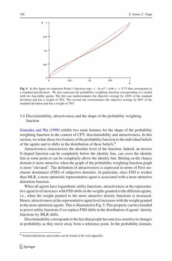
and ω (p) = exp − (− log pγ )) and estimate them through standard techniques. Fig-ure 4 permits to show that, with a well chosen distribution of agents’ characteris-tics, we obtain a distortion function that perfectly fits Prelec (1998)’s function. Wuand Gonzalez (1996, 1998), and Abdellaoui (2000) avoid the potential problems ofparametric estimation and directly derive from experimental studies the shape of theprobability weighting function at the aggregate or individual level. The results ofall these studies are (mostly) consistent with an inverse S-shaped weighting func-tion, concave for small probabilities, and convex for moderate and high probabili-ties.

In the lognormal setting, if we denote by δi the quantity δi = μi −μσ

, it is interestingto remark that the distortion function ge∗ only depends on the δi s and on the relativeproportions γi s and is independent of μ and σ . In other words, the distortion functiononly depends on how much the agents deviate from the objective mean in terms ofstandard deviation.

123


Fig. 4 In this figure we represent Prelec’s function exp(−(− ln p)γ ) with γ = 0.73 that corresponds toa standard specification. We also represent the probability weighting function corresponding to a modelwith two log-utility agents. The first one underestimates the objective average by 120% of the standarddeviation and has a weight of 30%. The second one overestimates the objective average by 60% of thestandard deviation and has a weight of 70%

3.4 Discriminability, attractiveness and the shape of the probability weightingfunction

Gonzalez and Wu (1999) exhibit two main features for the shape of the probabilityweighting function in the context of CPT: discriminability and attractiveness. In thissection, we relate these two features of the probability function to the individual beliefsof the agents and to shifts in the distribution of these beliefs.9

Attractiveness characterizes the absolute level of the function. Indeed, an inverseS-shaped function can be completely below the identity line, can cross the identityline at some point or can be completely above the identity line. Betting on the chancedomain is more attractive when the graph of the probability weighting function graphis more “elevated”. The definition of attractiveness is expressed in terms of First sto-chastic dominance (FSD) of subjective densities. In particular, since FSD is weakerthan MLR, a more optimistic representative agent is associated with a more attractivedistortion function.

When all agents have logarithmic utility functions, attractiveness at the representa-tive agent level increases with FSD shifts in the weights granted to the different agents,i.e., when the weight granted to the more attractive density functions is increased.Hence, attractiveness at the representative agent level increases with the weight grantedto the more optimistic agents. This is illustrated in Fig. 5. This property can be extendedto power utility functions if we replace FSD shifts in the distribution of agents’ densityfunctions by MLR shifts.

Discriminability corresponds to the fact that people become less sensitive to changesin probability as they move away from a reference point. In the probability domain,

9 Formal definitions and results can be found in the web appendix.

123


Fig. 5 In this figure we represent the probability weighting function of the representative agent in a modelwith logarithmic utility agents. In the upper curve, the optimistic and the pessimistic agents are equallyweighted. In the lower curve, the pessimistic agents have a 60% weight and the optimistic ones have a 40%weight. Attractiveness decreases with the weight granted to the pessimistic agents

Fig. 6 The probability weighting function for different levels of divergence of belief. Both agents agree ona normal distribution but one of them overestimates the objective mean by δ times the standard deviationwhile the other one underestimates it by δ times the standard deviation. The value of δ ranges from 0 to 2.The discriminability decreases with δ (in other words the curvature increases with δ)

the two endpoints 0 (certainly will not happen) and 1 (certainly will happen) serve asreference points and under this principle, increments near the endpoints of probabilityloom larger than increments near the middle of the scale.

When the level of disagreement among agents increases, then the representativeagent focuses more on the endpoints of the probability domain and is less sensitiveto probability variations in the middle of the scale. Figure 6 illustrates this result. Itshows, in the setting with two agents, that discriminability decreases with the level ofdisagreement. When both agents agree on the objective distribution, the probabilityweighting function is linear. When the agents disagree, one of them overestimating

123


the average payoff by twice the standard deviation and the other underestimating it bytwice the standard deviation, we obtain a function that approaches a step function.

4 Extensions and remarks

We have seen that starting from a standard model with optimistic as well as pessimis-tic vNM agents and a given aggregate endowment e∗, we obtain, at the representativeagent level, behavioral properties such as an inverse S-shaped distortion function ge∗ .These results can be extended in the following directions (see the web appendix formore detailed explanations).

4.1 Hyperbolic discounting

It has been shown in the literature that hyperbolic discounting is obtained at the aggre-gate level when one considers groups with heterogeneous exponential discount rates.This means that in the same way as we have obtained a behavioral bias on the beliefof the representative agent if heterogeneity of the beliefs is assumed at the individuallevel, a behavioral bias is obtained on the time preference rate of the representa-tive agent if heterogeneity of the time preference rates is assumed at the individuallevel. This result has been obtained in the literature through different approaches:Reinschmidt (2002) or Weitzman (1998, 2011) have adopted a certainty equivalentapproach, Gollier and Zeckhauser (2005) and Nocetti et al. (2008) a Benthamite/Paretooptimal approach, and Lengwiler (2005) an equilibrium approach. All these papersare in a deterministic setting, with no divergence in the beliefs of the agents. In oursetting, by assuming heterogeneity on the beliefs (as in Sect. 3) and on the timepreference rates of the agents, we can retrieve the behavioral properties at the aggre-gate level both on the belief of the representative agent and on her time preferencerate.

4.2 Cumulative prospect theory

In Sect. 3, the individual beliefs were given independently of the aggregate endow-ment e∗ and the distortion function ge∗ was specific to e∗. A dual approach consists inconsidering specific individual beliefs Qi , in order to obtain a distortion function thatis independent of a given aggregate endowment (or a given prospect) e∗ as in CPT.

Consider first the space E of normal distributions, and suppose that for all e∗ inE with e∗ ∼ N (μ, σ 2), the belief Qi,e∗ of agent i is such that e∗ ∼Qi,e∗ N (μi , σ

2)

with μi = μ + δiσ for some parameter δi . Then we can show that the representativeagent is a CPT agent over the space E of normal distributions, in the sense that thereexists a probability weighting function gδ such that for all e∗ in E with density fe∗ ,we have U (e∗) = ∫

fe∗,δ (s) u (s) ds where gδ

(∫ ∞t fe∗ (s) ds

) = ∫ ∞t fe∗,δ (s) ds;

moreover, if there exist at least one pessimistic and one optimistic agent, then thedistortion function gδ is inverse S-shaped.

123


This result can be easily extended to general distributions to obtain a CPT agentover the space of all random variables, by relying on the fact that any random variableis distributed as a function of a given normally distributed variable.

4.3 Dynamic issues

Our model might be embedded in a dynamic setting. Consider as in financial models adiffusion setting. We denote by W a Brownian motion and we assume that e∗ followsthe stochastic differential equation with constant parameters de∗

t = (μ + 1

2σ 2)

e∗t dt +

σe∗t dWt . The distribution of e∗

t is then, for all t, lognormal of the form log e∗t ∼

N (μt, σ 2t). Let us assume as in Sect. 4.2 that agents’ deviation from the objectivemean is constant in terms of standard deviation, i.e., that the subjective distributionsare of the form log N (μi t, σ 2t) with μi t = μt + δiσ

√t . There exists a probability

weighting function gδ that distorts the objective distribution into the distribution of thegroup. We check that this function is independent of t and the behavior of the groupis then consistent across time.

5 Appendix

5.1 Proofs of the main paper propositions

Proof of Proposition 1 At the Pareto optimum, we have

λi Mi u′(yi ) = q

for some random variable q. It follows that

yi =[

q

λi Mi

]−η

hence

e∗ =∑

i∈I

[q

λi Mi

]−η

= q−η∑

i∈I

[1

λi Mi

]−η

and

yi = e∗[λi Mi

]η∑

i∈I

[λi Mi

]η .

We have then

∑

i∈I

λi E[

Mi u(yi )]

=∑

i∈I

λi E

⎡

⎣Mi

[λi Mi

]η−1

(∑i∈I

[λi Mi

]η)1− 1η

u(e∗)

⎤

⎦

123


= E

⎡

⎣∑

i∈I

[λi Mi

]η

(∑i∈I

[λi Mi

]η)1− 1η

u(e∗)

⎤

⎦

= E

⎡

⎣

[∑

i∈I

[λi Mi

]η]1/η

u(e∗)

⎤

⎦

and U (e∗) = E[Mu(e∗)

]with M = [∑

i∈I ληi

(Mi

)η]1/η. ��

Proof of Corollary 2 We have

E[Mh

(e∗)] = E

⎡

⎣

(∑

i∈I

γi

(Mi

)η)1/η

h(e∗)

⎤

⎦

= E

⎡

⎣

(∑

i∈I

γi

(f i

f

(e∗)

)η)1/η

h(e∗)

⎤

⎦

= E

[(∑i∈I γi

(f i (e∗)

)η)1/η

f (e∗)h

(e∗)

]

=∫ (∑

i∈I γi(

f i (x))η)1/η

f (x)h (x) f (x) dx

=∫ (

∑

i∈I

γi

(f i (x)

)η)1/η

h (x) dx

hence f M = (∑i∈I γi ( fi )

η)1/η

. ��Proofs for Example 2 1. Proof that the distribution of log e∗ is bimodal for

|μ1 − μ2| > 2σ/√

η and unimodal for |μ1 − μ2| ≤ 2σ/√

η. We have

(f log

)η = 1

2

(f log1

)η + 1

2

(f log2

)η = 1

2√

2πσexp

(

−η (x − μ1)2

2σ 2

)

+ 1

2√

2πσexp

(

−η (x − μ2)2

2σ 2

)

.

This function has either two maxima that are symmetric with respect to μ1+μ22 or

only one maximum at μ1+μ22 . In the first case μ1+μ2

2 would be a local minimum.It suffices then to analyse the sign of the second derivative of

(f log

)ηat μ1+μ2

2 .

We obtain that the distribution is bimodal for |μ1 − μ2| > 2σ/√

η and unimodalfor |μ1 − μ2| ≤ 2σ/

√η.

2. Proof that for μ = μ1+μ22 the distribution of log e∗ is portfolio dominated by the

objective distribution. The ratio between the density of log e∗ under Q and the

123


density of log e∗ under P is given by

f M log

f log (x) =(

1

2exp

(

η−2 (x − μ) (μ − μ1) + μ2 − μ2

1

2σ 2

)

+ 1

2exp

(

η−2x(μ − μ2) + μ2 − μ2

2

2σ 2

)) 1η

which is clearly symmetric with respect to μ, decreasing before μ and increasingafter μ. Moreover, since the distributions of log e∗ under Q and under P are bothsymmetric with respect to μ, we have E Q

[log e∗] = E P

[log e∗] = μ. These

properties give VarQ[log e∗] > VarP

[log e∗] (see Jouini and Napp 2008).

3. Proof that for general (μi ) , VarQ[log e∗] > VarP

[log e∗] . For general

(μi ) , f M log is symmetric with respect to μ1+μ22 which gives E Q

[log e∗] =

μ1+μ22 . Furthermore, we may apply the same reasoning as in 2. to compare the

distribution of log e∗ under Q with the distribution whose density is given by

1√2πσ

exp −(

x− μ1+μ22

)2

2σ 2 . We then have VarQ[log e∗] > σ 2 = VarP

[log e∗] .

4. Proof that a higher level of risk tolerance induces a Portfolio Dominated shift inthe representative agent distribution. For two different values η and η′ of the risk

tolerance parameter, it suffices to considerf M logη′

f M logη

and to apply the same reasoning

as in 2. ��Proof of Proposition 3 1. If lim∞

foptf = lim−∞

fpessf = ∞ and lim−∞

foptf =

lim∞fpess

f = 0 then the representative agent density function is such that

lim−∞ fMf = lim∞ fM

f = ∞ and fMf can not be monotone.

2. This is immediate according to lim−∞ fMf = lim∞ fM

f = ∞.

3. It suffices to remark that f M = f maxopt

(γ max

opt + ∑i=1,...,N

i �=opt

(fi

f maxopt

)η)1/η

. If fif maxopt

is nonincreasing for all i then

(γ max

opt + ∑i=1,...,N

i �=opt

(fi

f maxopt

)η)1/η

is bounded away

from 0 and ∞ in the neighborhood of ∞ and we have f M ∼∞ f maxopt . The result

at the neighborhood of −∞ is obtained similarly. ��Proof of Proposition 4 1. Let g be given by

∫ ∞u fM (x)dx = g

[∫ ∞u f (x)dx

]. We

have fM (x) = g′ [∫ ∞u f (x)dx

]f (u) and g′ [∫ ∞

u f (x)dx] = fM

f (u) . We also

have − f (u)g′′ [∫ ∞u f (x)dx

] =(

fMf

)′(u) which gives that the concavity of g is

governed by the sign of(

fMf

)′. Remark that

(fMf

)′is negative in a neighborhood

of −∞ and then that g′′ is positive and g is convex in a neighborhood of 1. Sim-

ilarly, we have that(

fMf

)′is positive in a neighborhood of ∞ and then that g′′

123


is negative and g is concave in a neighborhood of 1 . Finally,(

fMf

)′is a combi-

nation of exponentials where the decreasing exponentials have a negative weight

and the increasing exponentials have a positive weight. The function(

fMf

)′is

then increasing. The function g is then inverse S-shaped: concave then convex.2. Since g′ [∫ ∞

u f (x)dx] = fM

f (u), we have g′(0) = fMf (∞) = ∞. If g′′(0) is well

defined, we have g′′(0) < 0 and hence g′′(x) < 0 in a neighborhood of 0. Theprobability weighting function is then concave for small probabilities. The resultin the neighborhood of 1 is obtained similarly. ��

5.2 Formal definitions and results for Sect. 3.4

The definition of attractiveness is expressed in terms of First Stochastic Dominance(FSD). The probability weighting function g1 is more attractive than the probabilityweighting function g2 when the subjective density f1 dominates the subjective densityf2 in the sense of the FSD. In our setting, we will say that a (representative agent’s)distortion function g1 associated with a set I1 of agents is more attractive than a (rep-resentative agent’s) distortion function g2 associated with a set I2 of agents if f M

I1

dominates f MI2

in the sense of the FSD. Attractiveness of the distortion function isrelated to the level of optimism of the representative agent. In particular, since FSD isweaker than MLR, a more optimistic representative agent is associated with a moreattractive distortion function.

Let (γi ) and(γ ′

i

)denote two possible distributions of agents’ density functions. If

the set ( fi )i∈I of agents’ density functions is totally ordered with respect to the FSDorder, we will say that the distribution

(γ ′

i

)dominates the distribution (γi ) in the sense

of the FSD if for any increasing family ( fi ) , we have∑

γ ′i fi �FSD

∑γi fi . In other

words, the distribution(γ ′

i

)puts more weight on more attractive distributions. If the

set ( fi )i∈I of agents’ density functions is totally ordered with respect to the optimismorder �opt, we will say that the distribution

(γ ′

i

)dominates the distribution (γi ) in

the sense of the MLR if whenever fi �opt f j we haveγ ′

iγi

≥ γ ′j

γ j. In other words, the

ratio between the two densities(γ ′

i

)and (γi ) increases with agents’ optimism and, in

particular, the distribution(γ ′

i

)puts more weight on more optimistic agents.

In the next proposition we analyze the impact of shifts in the distribution of agentscharacteristics on the attractiveness of the distortion function and on the level ofoptimism of the representative agent.

Proposition 5 1. For log-utility functions and in the case of lognormal distributionslog e∗ ∼Qi N (

μi , σ2)

for i = 1, ..., N , with the same variance parameter σ 2,a FSD shift in the distribution of the means (μi ) increases attractiveness of therepresentative agent’s distortion function.

2. For log-utility functions and general distributions, if the set ( fi )i∈I of agents’density functions is totally ordered with respect to the FSD order then a FSDshift in the distribution of agents’ density functions increases attractiveness of therepresentative agent’s distortion function.

123


3. For general CARA utility functions and general distributions, if the set ( fi )i∈Iof agents’ density functions is totally ordered with respect to the optimism order�opt then a MLR dominated shift in the distribution of agents’ density functionsincreases attractiveness of the representative agent’s distortion function and thelevel of pessimism of the representative agent.

Proof 1. Let us consider a distribution of the means that is described by a den-sity function h. The associated representative agent cumulative distribution

function is given by 1√2πσ 2

∫dh (μ)

∫ x−∞ exp − (s−μ)2

2σ 2 ds. Since the function

μ → ∫ x−∞ exp − (s−μ)2

2σ 2 ds is decreasing a FSD shift of h decreases the value

of∫

dh (μ)∫ x−∞ exp − (s−μ)2

2σ 2 ds and leads then to a FSD dominating distributionfunction for the representative agent.

2. Let us consider a distribution(γ ′

i

)and a FSD dominated shift (γi ). We want to

prove that∑

γ ′i Fi ≥ ∑

γi Fi . For a given x, letting xi denote the quantity Fi (x), itsuffices to prove that

∑γ ′

i xi ≥ ∑γi xi for a nondecreasing family (xi )i∈I which

is true since(γ ′

i

)dominates (γi ) in the sense of the FSD.

3. Let us consider a distribution(γ ′

i

)and a MLR dominated shift (γi ). It suffices

to prove that (∑

γ ′i f η

i )1η

(∑

γi f ηi )

1η

is increasing or that∑

γ ′i Gi∑

γi Giis increasing with Gi = f η

i .

Without any loss of generality, we may assume that all the considered functions

are differentiable and let us consider the derivative of∑

γ ′i Gi∑

γi Gi

(∑γ ′

i Gi∑γi Gi

)′=

(∑γ ′

i G ′i

) (∑γi Gi

) − (∑γ ′

i Gi) (∑

γi G ′i

)

(∑γi Gi

)2

=∑

fi � f jγiγ j

(γ ′

iγi

− γ ′j

γ j

)(G ′

i G j − Gi G ′j

)

(∑γi Gi

)2 .

Remark that for fi � f j we have Gi � G j and then G ′i G j −Gi G ′

j ≥ 0. Furthermore,

for fi � f j we also haveγ ′

iγi

− γ ′j

γ j≥ 0 which leads to the conclusion. ��

When all agents have logarithmic utility functions, attractiveness at the represen-tative agent level increases with the weight granted to the more attractive densityfunctions. Since FSD is weaker than MLR, attractiveness at the representative agentlevel increases with the weight granted to the more optimistic agents. This is illustratedby Fig. 5. As shown in Proposition 5, this last property can be extended to power utilityfunctions if we replace FSD shifts on the distribution of agents’ density functions byMLR shifts.

Diminishing sensitivity corresponds to the fact that people become less sensitive tochanges in probability as they move away from a reference point. In the probabilitydomain, the two endpoints 0 (certainly will not happen) and 1 (certainly will happen)serve as reference points and under this principle, increments near the endpoints of

123


probability loom larger than increments near the middle of the scale. This concept isrelated to the concept of discriminability in psychophysics literature and can be illus-trated by two extreme cases: a function that approaches a step function and a functionthat is almost linear.

In our setting we say that a representative agent’s distortion function g1 associatedwith a set I1 of agents exhibits more discriminability than a representative agent’sdistortion function g2 associated with a set I2 of agents if there exists x∗ ∈ [0, 1] suchthat g1 ≤ g2 for x ≤ x∗ and g1 ≥ g2 for x ≥ x∗. In the next proposition we show thatthe level of discriminability of the representative agent’s distortion function is closelyrelated to the level of disagreement among agents.

Let us consider as above a family of agents with lognormal distributionsln N (μi , σ

2). We denote by (μi ) the support of the distribution of the mean parameterand by (γi ) the associated weights. Recall that a mean preserving spread is defined asa modification of the distribution set (γi ) on a set of three locations μ1 < μ2 < μ3with associated increments δ1 ≥ 0, δ2 ≤ 0 and δ3 ≥ 0 such that

∑3i=1 δi = 0 and

∑3i=1 δiμi = 0. A mean preserving spread will be said symmetric if δ1 = δ3.

Proposition 6 For log-utility functions and in the case of lognormal distributionslog e∗ ∼Qi N (μi , σ

2), a symmetric mean-preserving spread on the distribution ofthe means (μi ) decreases discriminability of the representative agent’s distortionfunction.

Proof It is immediate that μ1, μ2, and μ3 can be written in the form μ2−h, μ2, μ2+hfor some h > 0. For the distribution of individual characteristics (γi ) , the represen-

tative agent distribution function is given by 1√2πσ 2

∑i γi

∫ x−∞ exp − (s−μi )

2

2σ 2 ds. Thesymmetric mean preserving spread induces a modification of this distribution that

is positively proportional to 1√2πσ 2

(∫ x−∞ exp

(− (s−μ2+h)2

2σ 2

)− 2 exp

(− (s−μ2)2

2σ 2

)+

exp(− (s−μ2−h)2

2σ 2

))ds. Simple computations permit to show that this modification is

positive for x ≤ μ2 and negative for x ≥ μ2. A symmetric mean preserving spreadleads then to a distribution function that is above (resp. below) the original distri-bution function below a given threshold. We have then an increase of the level ofdiscriminability. ��

Intuitively, this proposition means that when the level of disagreement among agentsincreases, then the representative agent focuses more on the endpoints of the proba-bility domain and is less sensitive to probability variations in the middle of the scale.Figure 6 illustrates this result. It shows, in the setting with two agents, that discrim-inability decreases with the level of disagreement. When both agents agree on theobjective distribution, the probability weighting function is linear. When the agentsdisagree, one of them overestimating the average payoff by twice the standard devi-ation and the other underestimating it by twice the standard deviation, we obtain afunction that approaches a step function.

123



In this section, we extend our framework in order to take into account the impact oftime and of heterogeneous time preference rates across the agents. Aggregate endow-ment at a given date t is described by a random variable e∗

t . Agents have different timepreference rates (ρi ) and different subjective beliefs Qi . We let Mi

t denote the densityat date t of Qi with respect to the objective probability P and Di

t ≡ exp (−ρi t) thediscount factor of agent i between date 0 and date t . As previously, we consider theaggregate utility function U defined as the solution of the following maximizationprogram

U (e∗t ) = max∑

i∈I yit =e∗

t

∑

i∈I

λi E[

Mit Di

t u(yit )

]

where (λi ) are given positive weights. Each agent is then characterized by a beliefMi

t , a discount factor Dit and a weight λi .

We will say that the characteristics(Mi

t , Dit , λi

)i∈I are independent if for almost

all states of the world ω, Mit (ω) , Di

t and λi are independent10 as random variableson I. This property will be, in particular, satisfied when I can be written in the form

I = J × K × L and when there exist characteristics(

M̄ jt

)

j∈J,(D̄k

t

)k∈K and

(λ̄�

)�∈L

such that for i = ( j, k, �) we have(Mi

t , Dit , λi

) =(

M̄ jt , D̄k

t , λ̄�

). Roughly speak-

ing, this property means that there is no specific correlation between beliefs and timepreferences and that the weights granted by the social planner to the individuals in theeconomy are independent of their time and belief characteristics.

This condition is, in particular, satisfied when beliefs and time preferences are inde-pendent and when the agents are uniformly weighted in the social welfare function.This is also the case when the agents’ weights are given by their relative wealth andwhen wealth, beliefs and time preferences are independent.

Assuming uniform weights is quite reasonable since there is no particular reasonfor the social planner to favor one agent with respect to another agent. The indepen-dence of beliefs and time preference rates is more disputable. They may be positivelyas well as negatively correlated, the independence condition may then be analyzed asa central scenario.

We easily obtain the following analog of Proposition 1 in the framework withheterogeneous time preference rates.

Proposition 7 If the characteristics(Mi

t , Dit , λi

)i∈I are independent, then the aggre-

gate utility for consumption is given by

U (e∗t ) = E

[Mt Dt u(e∗

t )]

10 More precisely, for any real valued (measurable) functions f, g, h defined on the real line, we have

1|I |

∑

i∈If(

Mit

)g

(Di

t

)h (λi ) =

(1|I |

∑

i∈If(

Mit

))(1|I |

∑

i∈Ig

(Di

t

))(1|I |

∑

i∈Ih (λi )

)

a.e.

123


with

Mt =(

1

|I |∑

i∈I

(Mi

t

)η) 1

η

and Dt =(

1

|I |∑

i∈I

(Di

t

)η) 1

η

.

The representative agent belief is then given by Mt =(

1|I |

∑i∈I

(Mi

t

)η) 1

ηand the

representative agent time discount factor is given by Dt =(

1|I |

∑i∈I

(Di

t

)η) 1

η.

Proof Replacing Mi by Mi Di in the proof of Proposition 1, we easily get that

U(e∗

t

) =[∑

i∈I

[λi Mi

t Dit

]η]1/η

.

Now, if the characteristics(λi , Mi

t , Dit

)are independent, then

[∑

i∈I

[λi Mi

t Dit

]η]1/η

=[(

1

|I |∑

i∈I

(Mi

t

)η)]1/η [(

1

|I |∑

i∈I

(Di

t

)η)]1/η

and

∑

i∈I

λi E[

Mit Di

t u(yit )

]= E

⎡

⎣

(1

|I |∑

i∈I

(Mi

t

)η)1/η (

1

|I |∑

i∈I

(Di

t

)η)1/η

u(e∗t )

⎤

⎦ .

��This means that all the properties established in the previous section on the belief

of the representative agent remain valid.The properties of the representative agent time preference rate are easy to obtain.

Note that the properties of a “consensus” time preference rate when there is hetero-geneity on the individual time preference rates (and not on the beliefs) have alreadybeen studied in varying contexts. Indeed, the problem of the aggregation of the utilitydiscount rates has been studied by Reinschmidt (2002) through a certainty equiva-lent approach, by Gollier and Zeckhauser (2005) and Nocetti et al. (2008) through aBenthamite/Pareto optimal approach, and by Lengwiler (2005) through an equilib-rium approach. All these papers adopt a deterministic setting with no divergence onthe beliefs of the agents. On the contrary our aim here is to derive the properties at theaggregate level simultaneously on the beliefs and on the time preference rate (and ina quite general stochastic setting).

We know that the representative agent time discount factor is given by Dt =(∑

i∈I1|I |

(Di

t

)η) 1

ηwhere Di

t ≡ exp (−ρi t) . We introduce the representative agent

123


marginal time preference rate ρm as well as the representative agent average timepreference rate ρa, respectively defined by

ρDm (t) ≡ − D′

t

Dtand ρD

a (t) ≡ −1

tlog Dt .

The average discount rate corresponds to the rate which, if applied constantly forall intervening years, would yield the discount factor Dt, whereas the marginal dis-count rate is the rate of change of the discount factor. It is easy to recover the averagediscount rate from the marginal discount rate since ρa (t) = 1

t

∫ t0 ρm (s) ds.

Let us state the following properties of the average and marginal time preferencerates.

Proposition 8 Properties of the representative agent time preference rate

1. The representative agent average and marginal time preference rates are givenby

ρDa (t) = −1

tlog

[1

N

N∑

i=1

exp (−ηρi t)

]1/η

,

ρDm (t) =

N∑

i=1

exp (−ηρi t)∑N

i=1 exp (−ηρi t)ρi .

2. The representative agent time preference rates are lower than the average of thetime preference rates, i.e.

ρDm (t) ≤ 1

N

N∑

i=1

ρi = ρDm (0) and ρD

a (t) ≤ 1

N

N∑

i=1

ρi = ρDa (0)

with strict inequalities when ρi �= ρ j for some (i, j) in I .3. “Behavioral Properties” : The representative agent time preference rates are

decreasing with time. Moreover, the asymptotic discount rates are given by thelowest time preference rate, i.e. limt→+∞ ρD

a (t) = limt→+∞ ρDm (t) = inf i (ρi ) .

The representative agent behaves for t large enough like the most patient agent.

Proof We prove the proposition for ρDm since it is easy to check that all the derived

properties are inherited by ρDa (t) = 1

t

∫ t0 ρD

m (s) ds.

1. Immediate.2. The representative agent time preference rate ρD

m (t) = ∑Ni=1

exp(−ηρi t)∑Ni=1 exp(−ηρi t)

ρi

is an average of the ρi s with weights that decrease with ρi . Such an average issmaller than the equally weighted average.

3. Denote θi = exp (−ηρi t). We have dρDm (t)dt = −

(∑i∈I θi ρ

2i∑

i∈I θi−

(∑i∈I θi ρi∑

i∈I θi

)2)

which

is negative.

123


We have ρDm (t)= ρinf+∑N

i �=inf exp(−η(ρi −ρinf )t)ρi

1+∑Ni �=inf exp(−η(ρi −ρinf )t)

and exp (−η(ρi−ρinf)t) ρi →∞ 0

we have then ρDm (t) → ρinf . ��

These formulas permit explicit computations for specific distributions of the indi-vidual time preference rates. For instance, if we assume a Gamma 11 distributionγ (α, β) for the ρi s we obtain

ρDm (t) = m2

m + ηv2t

where m and v2 respectively denote the mean and the variance of the considereddistribution. It is immediate on this simple example that the marginal discount ratedecreases with time and is hyperbolic as in Weitzman (1998, 2011). Furthermore, thespeed of the decrease increases with the level of heterogeneity v2 as well as with thelevel of risk tolerance.

The next proposition provides comparative statics results for shifts in the distribu-tion fρ of the individual time preference rates.

Proposition 9 1. A FSD (resp. SSD) dominated shift in the distribution fρ ofindividual time preference rates decreases the representative agent average timepreference rate ρD

a .

2. A MLR (resp. PD) dominated shift in the distribution fρ of individual time pref-erence rates decreases the representative agent marginal time preference rateρD

m .

Proof The proof of 1. is inspired from Jouini and Napp (2008) and the proof of 2. isinspired from Nocetti et al. (2008).

1. We have

ρDa (t) ≡ − 1

ηtln E

[exp (−ηρt)

]

where E is the expectation operator associated with the distribution of (ρi ). Fora given t, the function ρ → exp (−ηρt) is decreasing (and convex) and, by def-inition, a FSD (resp. SSD) shift in the distribution of (ρi ) decreases the value ofE

[exp (−ηρt)

]and increases ρD

a (t) .

2. We have then

ρDm (t) = E

[ρ exp (−ηρt)

]

E[exp (−ηρt)

] .

where E is the expectation operator associated with the distribution of (ρi ) .

11 As mentioned in Sect. 2, sums should be replaced by integrals when dealing with continuous distribu-

tions. The density function of a gamma distribution γ (α, β) is given by βα

�(α)xα−1 exp(−βx). Its mean m

and its variance v2 are respectively given by m = αβ and v2 = α

β2 .

123


1. Let us now consider P1andP2, two distributions such that P2 �MLR P1. Bydefinition, the density φ = dP2

dP1 is nondecreasing in ρ (in other words i → φi and

i → ρi are comonotonic). We have then, E P2 [ρ exp(−ηρt)]E P2 [exp(−ηρt)]

= E P1 [φρ exp(−ηρt)]E P1 [φ exp(−ηρt)]

=E Q [φρ]E Q [φ]

where Q is defined by a density with respect to P1 equal (up to a constant)to exp (−ηρt) . Since φ is nondecreasing in ρ, we have

E Q [φρ] ≥ E Q [φ] E Q [ρ] ,

hence

E P2 [ρ exp (−ηρt)

]

E P2 [exp (−ηρt)

] ≥ E Q [ρ] ,

≥ E P1 [ρ exp (−ηρt)

]

E P1 [exp (−ηρt)

] .

Let us assume now that P2 �P D P1 and let us consider ρD,P2

m (t) and

ρD,P1

m (t) the associated representative agent time preference rates. We have

ρD,P2

m (t)= E P2 [ρ exp(−ηρt)]E P2 [exp(−ηρt)]

and then E P2[u′(ρ)(ρ − ρ

D,P2

m )]=0 with u(ρ)=−

exp(−ηρt). By definition, this implies E P1[u′(ρ)(ρ − ρ

D,P2

m )]

≤ 0 hence

ρD,P2

m ≥ ρD,P1

m . ��Second Stochastic dominance as well as portfolio dominance are related to a notion

of risk or of dispersion while first Stochastic dominance and Monotone likelihood ratiodominance are related to notions of shifts from low values to high values. Roughlyspeaking, Proposition 9 introduces the right concepts of dispersion and shifts andshows that more dispersion in agents’ time preference rates as well as shifts to lowervalues of individual time preference rates decrease the representative agent’s timepreference rate.


In this section we show that an individual who evaluates lotteries through the socialwelfare function associated with a collection of agents, each of them with specificnoisy beliefs, distorts the distribution of the lotteries through an inverse S-shapedweighting function (common to all lotteries) as in CPT.

We start by considering normal distributions. Let us consider an individual whowhen facing a lottery whose payoff x is described by a normal distribution N (μ, σ 2)

passes this information for evaluation to separate systems. Each system i has a subjec-tive belief Qi under which x has a normal distribution N (

μ + δiσ, σ 2). The parameter

δi is fixed independently of x and characterizes the system i . It might result from noisein the information transmission. In that case there is no specific reason for the average

123


perceived signal to be biased and we should have∑

δi = 0. We assume that theindividual acts like a central planner looking for a Pareto optimal decomposition ofthe payoffs from the lottery among the systems and evaluates the lottery through thesocial welfare function, i.e.,

Uδ(x) = max∑xi =x

∑

i

γi E Qi[u(xi )

](2)

where the parameters γi are the weights granted to the systems by the central planneror the distribution of the δi s.

Proposition 10 Consider an individual who evaluates any lottery x in the space X oflotteries with normal payoffs through Uδ(x).

1. The individual is a CPT agent over the space X in the sense that there exists aprobability weighting function gδ such that, for all lotteries x in X with densityfx we have Uδ(x) = ∫

fx,δ(s)u (s) ds where gδ(∫ ∞

t fx (s)ds) = ∫ ∞t fx,δ(s)ds.

2. If there exist at least one optimistic and one pessimistic system, then gδ is inverseS-shaped.

3. A MLR shift on the distribution of the δi s increases attractiveness of the probabilityweighting function gδ .

Proof 1. Let x ∈ X with x ∼ N (μ, σ 2

). We have x ∼Qi N (

μ + δiσ, σ 2).

From Proposition 1, there exists Q such that Uδ(x) = E Q [x] and the density

of x under Q is given by fx,δ (s) =[

1n

∑Ni=1

(fx,δi

)η]1/η

where fx,δi is the

density of x under Qi . We then have Uδ(x) = ∫fx,δ(s)u (s) ds. It suffices to

prove that∫ ∞

t fx,δ(s)ds is a function of∫ ∞

t fx (s)ds that does not depend onx, i.e. that does not depend upon μ and σ. Let gδ be the function defined by

gδ

(1√2π

∫ ∞t exp

(− x2

2

)ds

)= ∫ ∞

t

[1n

∑Ni=1

(1√2π

exp(−η

(x−δi )2

2

))]1/η

ds for

all t. The function gδ is completely defined on [0, 1] and by a simple change of

variables, we have gδ

(1√

2πσ

∫ ∞t exp

(− (x−μ)2

2σ 2

)ds

)= ∫ ∞

t

[1n

∑Ni=1

(1√

2πσexp

(− η

(x−δi σ−μ

)2

2σ 2

))]1/η

ds for all t and we then have∫ ∞

t fx,δ(s)ds =gδ

(∫ ∞t fx (s)ds

).

2. The function gδ is the same as in Proposition 4.3. Direct application of Proposition 5. ��This means that a Pareto optimal decomposition leads to an overall (representativeagent) evaluation that corresponds to the valuation that would be provided by a behav-ioral agent. The level of discriminability would then be directly related to the level ofnoise as illustrated in Proposition 6 in the case of log utility functions. The level ofattractiveness would be associated to the level of systematic bias (if any) as a directcorollary of Proposition 5.

123


The behavior of the individual and the definition of the social welfare function Uδ

can be naturally generalized to any lottery whose payoff is a function of a normaldistribution. Indeed, consider a lottery whose payoff is of the form v = ϕ(x) where xis normally distributed as above and where ϕ is a Borelian function. We may defineUδ(v) by

Uδ(v) = max∑vi =v

∑

i

γi E Qi[u(vi )

]

where the Qi s and the δi s are the same as for x .The following result extends the result of Proposition 10 to general lotteries. It relies

on the fact that any random variable is distributed as a function of a given normallydistributed variable.

Proposition 11 Consider an individual who evaluates through Uδ any lottery v =ϕ(x) where x is normally distributed and whose preferences over the set of all pos-sible lotteries only depend on the distribution of the lottery under consideration. Theindividual is a CPT agent over the space of all possible lotteries in the sense that herpreferences can be represented by the utility function Uδ extended to the space of allpossible lotteries and there exists a probability weighting function gδ such that, for alllottery v with density fv we have Uδ(v) = ∫

fv,δ(s)u (s) ds where gδ(∫ ∞

t fv(s)ds) =∫ ∞t fv,δ(s)ds.

Proof Let v such that v = ϕ(x) where x is normally distributed. By definition, wehave Uδ(v) = sup∑

viE Qi [u(vi )]. We denote by f i

v the density of v with respect

to Qi . By Proposition 1 and Corollary 2, we have Uδ(v) = ∫fv,δ(s)u (s) ds with

fv,δ = (∑(f iv

)η) 1η . We clearly have fv,δ = ϕ′ fx,δ ◦ ϕ and f i

v = ϕ′ f ix ◦ ϕ and

since∫ ∞

t fx,δ(s)ds = ∫ ∞t

(∑(f ix

)η) 1η (s)ds = gδ

(∫ ∞t fx (s)ds

), a simple change

of variable leads to∫ ∞

t fv,δ(s)ds = gδ

(∫ ∞t fv(s)ds

). We have then the result over

the set of transformations of normal distributions.Let us consider now a random variable v and a normally distributed random variable

x . We know that v has the same distribution as F−1v [Fx (x)] where F−1

v (p) is definedby F−1

v (p) = inf {t : Fv(t) ≥ p} . If the individual has preferences that only dependon the distribution, it suffices to set Uδ(v) = Uδ(ϕ(x)) with ϕ = F−1

v ◦Fx which is per-fectly defined. We then have Uδ(x) = ∫ ∞

t fϕ(x),δ(s)u(s)ds with∫ ∞

t fϕ(x),δ(s)ds =gδ

(∫ ∞t fϕ(x)(s)ds

)and since v is distributed like ϕ(x), we have

∫ ∞t fϕ(x),δ(s)ds =

gδ

(∫ ∞t fv(s)ds

), and the result follows. ��

This corollary provides then the following possible interpretation of CPT: the resultof a possibly noisy transmission of the objective distribution to separate (specialized)systems, the overall evaluation resulting from a social welfare function applied tothese systems. The construction of the Qi s in the general case is very similar to theirconstruction in the normal case. The resulting global behavior might then be associ-ated intuitively with a possible behavior of the systems that consists in describing anyrandom variable in terms of Gaussian distributions. For instance, a random variable

123


that takes values 0 and 1 with probability 1/2 may be described as a random variablethat takes value 1 when a given Gaussian variable N (0, 1) is positive and that takesvalue 0 when the Gaussian variable is negative. The process i will then transform thisbinomial distribution into a binomial distribution that is equal to 1 when a Gaussianvariable N (δi , 1) is positive -or equivalently when a Gaussian variable N (0, 1) issmaller than δi - and is equal to 0 when the Gaussian variable N (δi , 1) is negative.

References

Abel, A. (2002). An exploration of the effects of pessimism and doubt on asset returns. Journal ofEconomic Dynamics and Control, 26, 1075–1092.

Abdellaoui, M. (2000). Parameter-free elicitation of utilities and probability weighting functions.Management Science, 46, 1497–1512.

Abdellaoui, M., L’Haridon, O. & Paraschiv, C. (2010). Individual vs collective behavior: An experimentalinvestigation of risk and time preferences in couples, Working Paper.

Chateauneuf, A., & Cohen, M. (1994). Risk seeking with diminishing marginal utility in a nonexpectedutility model. Journal of Risk and Insurance, 9, 77–91.

Chiappori, P-A. (1988). Nash-bargained households decisions: A comment. International EconomicReview, 29, 791–796.

Chiappori, P-A. (1992). Collective labor supply and welfare. Journal of Political Economy, 100, 437–467.Chiappori, P.-A., Samphantharak, K., Schulhofer-Wohl, S. & Townsend, R. (2010). Heterogeneity and

risk sharing in Thai villages, Working Paper.Diecidue, E. & Wakker, P. (2001). On the intuition of rank dependent utility. Journal of Risk and

Insurance, 281–298.Gollier, C. (1997). A note on portfolio dominance. Review of Economic Studies, 64, 147–150.Gollier, C., & Zeckhauser, R. (2005). Aggregation of heterogeneous time preferences. Journal of Political

Economy, 113(4), 878–898.Gonzalez, R., & Wu, G. (1999). On the shape of the probability weighting function. Cognitive

Psychology, 38, 129–166.Jouini, E., & Napp, C. (2007). Consensus consumer and intertemporal asset pricing with heterogeneous

beliefs. Review of Economic Studies, 74, 1149–1174.Jouini, E., & Napp, C. (2008). On Abel’s concept of doubt and pessimism. Journal of Economic

Dynamics and Control, 32, 3682–3694.Landsberger, M., & Meilijson, I. (1990). Demand for risky assets: A portfolio analysis. Journal of

Economic Theory, 50, 204–213.Landsberger, M., & Meilijson, I. (1993). Mean preserving portfolio dominance. The Review of Economic

Studies, 60, 475–485.Lengwiler, Y. (2005). Heterogeneous patience and the term structure of real interest rates. American

Economic Review, 95, 890–896.Loewenstein, G., & Prelec, D. (1992). Anomalies in intertemporal choices: Evidence and an interpre-

tation. The Quarterly Journal of Economics, 107, 573–597.Lopes, L. (1987). Between hope and fear: The psychology of risk. Advances in Experimental Social

Psychology, 20, 255–295.Luce, R. D. (1996). When four distinct ways to measure utility are the same. Journal of Mathematical

Psychology, 40, 297–317.Mazzocco, M. & Saini, S. (2011) Testing efficient risk sharing with heterogeneous risk preferences.

American Economic Review, (forthcoming).Nocetti, D., Jouini, E., & Napp, C. (2008). Properties of the social discount rate in a Benthamite

framework with heterogeneous degrees of impatience. Management Science, 54, 1822–1826.Prelec, D. (1998). The probability weighting function. Econometrica, 66, 497–527.Reinschmidt, K. F. (2002). Aggregate social discount rate derived from individual discount rates. Man-

agement Science, 48, 307–312.Shefrin, H. (2005). A behavioral approach to asset pricing. Elsevier.Tversky, A., & Fox, C. R. (1995). Ambiguity aversion and comparative ignorance. Quarterly Journal

of Economics, 110, 585–603.

123


Tversky, A., & Kahneman, D. (1992). Advances in prospect theory: Cumulative representation ofuncertainty. Journal of Risk and Uncertainty, 5, 297–323.

Ulf, D. (1988). A general non cooperative Nash model of household consumption behavior, WorkingPaper 88–205, Department of Economics, University of Bristol.

Weitzman, M. (1998). Why the far distant future should be discounted at its lowest possible rate. Journalof Environmental Economics and Management, 36, 201–208.

Weitzman, M. (2001). Gamma discounting. The American Economic Review, 91, 260–271.Wu, G., & Gonzalez, R. (1996). Curvature of the probability weighting function. Management Sci-

ence, 42, 1676–1690.Wu, G., & Gonzalez, R. (1998). Common consequence conditions in decision making under risk. Journal

of Risk and Uncertainty, 16, 115–139.Yaari, M. E. (1987). The dual theory of choice under risk. Econometrica, 55, 95–115.

123

behavioral biases and the representative agent

Documents