ARTICLE

Received 17 Oct 2014 | Accepted 29 Jan 2015 | Published 10 Mar 2015

Beating beats mixing in heterodyne detectionschemesG.J. Verbiest1 & M.J. Rost2

Heterodyne detection schemes are widely used to detect and analyse high-frequency signals,

which are unmeasurable with conventional techniques. It is the general conception that the

heterodyne signal is generated only by mixing and that beating can be fully neglected, as it is

a linear effect that, therefore, cannot produce a heterodyne signal. Deriving a general

analytical theory, we show, in contrast, that both beating and mixing are crucial to explain

the heterodyne signal generation. Beating even dominates the heterodyne signal, if the

nonlinearity of the mixing element (mixer) is of higher order than quadratic. The specific

characteristic of the mixer determines its sensitivity for beating. We confirm our results with

both a full numerical simulation and an experiment using heterodyne force microscopy, which

represents a model system with a highly non-quadratic mixer. As quadratic mixers are the

exception, many results of previously reported heterodyne measurements may need to be

reconsidered.

DOI: 10.1038/ncomms7444

1 JARA-FIT and II. Institute of Physics, RWTH Aachen University, 52074 Aachen, Germany. 2 Huygens-Kamerlingh Onnes Laboratory, Leiden University,Niels Bohrweg 2, 2333 CA Leiden, The Netherlands. Correspondence and requests for materials should be addressed to G.J.V.(email: Verbiest@physik.rwth-aachen.de) or to M.J.R. (email: Rost@physics.leidenuniv.nl).

NATURE COMMUNICATIONS | 6:6444 | DOI: 10.1038/ncomms7444 | www.nature.com/naturecommunications 1

& 2015 Macmillan Publishers Limited. All rights reserved.

There are many periodic processes with such a highfrequency that they are difficult to measure experimentally.A solution is the application of a heterodyne detection

scheme, as it down-converts the high-frequency signal to a lower,easily measurable frequency by mixing it with a reference signal.This enables the quantification of the amplitude, the phase andthe frequency modulation of the original, high-frequency signal.A well-known example of a heterodyne detector is the radio.Heterodyne detection is also widely used in optics, in quantumdevices, in the detection of nuclear magnetic resonance, inmicrowave detection, in scanning tunnelling spectroscopy andeven in the search for gravitational waves1–7.

Despite the successful application of heterodyne detectionschemes, the exact generation of the heterodyne signal is oftennot well understood such that quantitative interpretations areonly possible with extensive numerical calculations. Moreover,until now it has not been realized that the standard textbookequation for mixing usually fails, as in reality almost all mixerscontain a beating stage at their input. To address this problem, wederived a general analytical theory that uses beating plus mixingfor the generation of the heterodyne signal such that it becomesvalid for all heterodyne detection schemes.

Although not recognized, almost all heterodyne mixers have asingle input channel, through which a superposition is realized ofthe high-frequency signal and the reference signal before the realnonlinear mixing takes place: in optics, for example, the measuredintensity is the square of the superposed electric fields.Consequently, we have to differentiate between beating, whichis a linear effect occurring for superpositions and mixingoccurring for nonlinear couplings.

In the following, we show that both beating and mixing arenecessary to correctly describe the generation of the heterodynesignal. By deriving a general analytic theory that we confirm withsimulations and experiments, we demonstrate that beating plays acrucial role in any type of heterodyne measurement system. Inparticular, we show that beating dominates mixing, if the mixer isof higher order than quadratic.

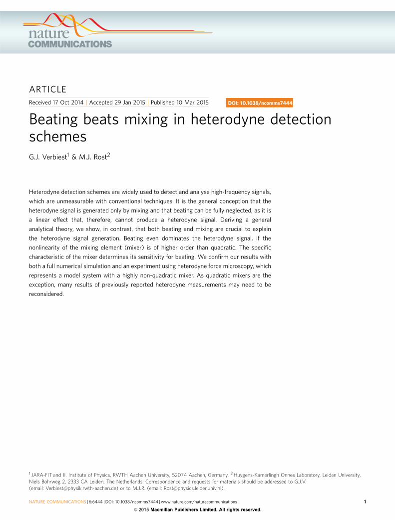
ResultsDifferentiating between Beating and Mixing. The upper panelof Fig. 1 depicts beating: it is the sum of two harmonic excitationsat frequencies os and ot. The result (black line) oscillates with afrequency oh (osoohoot) and beats in amplitude at the dif-ference frequency odiff¼ |os�ot| (red lines). However, as theFourier transform of the time trace only shows the two originalfrequencies os and ot, no signal is generated at the differencefrequency odiff. Mixing, see lower panel of Fig. 1, is the product oftwo or more harmonic excitations and occurs if the transferfunction of the mixer is of quadratic or higher order. This resultreally oscillates at the difference frequency (red line) and the sumfrequency (black line). In contrast to beating, the Fourier trans-form shows the difference and the sum frequency, but not the twofrequencies of the original harmonic excitations. Although beat-ing and mixing are two intrinsically different effects that areclassified by the type of mixer and their Fourier analyses, we willfully counterintuitively demonstrate that beating even dominatesmixing, if the mixer is of higher order than quadratic!

To illustrate the importance of beating in heterodynemeasurements, we use the example of heterodyne force micro-scopy (HFM)8–10, as it represents a model system with a highlynonlinear mixing element (much higher order than quadratic).HFM enables the non-destructive imaging below a surface withnanometre resolution using an atomic force microscope11–19. Thetypical excitation scheme is sketched in Fig. 2a. The subsurfaceinformation is contained in an ultrasonic sound wave thattravelled through the sample with a frequency os of several MHz

(well above the first resonance of the cantilever). To detect thissignal, one applies a heterodyne detection scheme and excites,therefore, also the cantilever/tip with a high frequency ot thatdeviates slightly from os. The nonlinear tip–sample interactiongenerates a heterodyne signal at a sufficiently low differencefrequency odiff such that the cantilever really starts to move atodiff. In this way, the tip–sample distance is the superposition ofthe sample vibration with amplitude As and phase fs, and thecantilever vibration with amplitude At and phase jt, on the basisof which the nonlinear tip–sample interaction generates thedifference frequency. Usually, one tunes odiff below the firstresonance of the cantilever, however, this choice is not necessary,as long as the difference frequency can still excite a real motion inthe cantilever. This information is provided by the transferfunction of the cantilever, as it describes the reaction of thecantilever for a given applied force as a function of the frequency.

Figure 2b depicts the heterodyne signal generation for theexample of HFM. The sum of the ultrasound signals atfrequencies ot and os results in beating at the mixer’s input.This mixer generates a heterodyne drive force at odiff, whichresults in a real motion of the cantilever via the cantilever’stransfer function H(odiff). HFM is special, as the output of thistransfer function (real motion at odiff) is coupled back into thetip–sample distance, which leads to an additional beating term atthe input of the mixer. The transfer function also acts as a filter,which eliminates almost any contribution from the sumfrequency |otþos|, as well as higher-order mixing terms:A|osþot|/A|osþot|¼ 0.004. We derive the transfer function inSupplementary Note 5.

We also address the general case without back coupling to themixer below, as well as in Supplementary Note 4, and show thatbeating still gives significant corrections to the heterodyne signal.Although the back coupling can, in principle, also alter theultrasonic amplitudes At and As (and corresponding phases), itwas surprisingly shown experimentally that At and As remainconstant for all tip–sample distances z in HFM20,21. Therefore,

Beating: As cos (�st ) + At cos (�tt )

Nonlinear mixing: As cos (�st ) × At cos (�tt )

Time trace

FT

Bea

ting

(nm

)N

onlin

ear

mix

ing

(nm

2 )

Time trace

FT

Time (μs) Frequency (MHz)

1

0

–1

10155 0,10 1

0.1

0

–0.1

(a.u

.)(a

.u.)

�t

| �s+�t || �s–�t |

�s

Figure 1 | Beating versus mixing. Beating is the sum of two harmonic

functions (upper panel): the Fourier transform (FT) contains only the two

original frequencies os and ot. Mixing is the product of two harmonic

functions (lower panel): the FT contains only the two nonlinear frequencies

|os�ot| and |osþot|. The graphs have been calculated for os¼ 1.1 MHz,

ot¼ 1 MHz, As¼0.1 nm and At¼ 1 nm.

ARTICLE NATURE COMMUNICATIONS | DOI: 10.1038/ncomms7444

2 NATURE COMMUNICATIONS | 6:6444 | DOI: 10.1038/ncomms7444 | www.nature.com/naturecommunications

& 2015 Macmillan Publishers Limited. All rights reserved.

HFM behaves exactly as a conventional heterodyne detectionscheme with an additional back coupling of only the differencefrequency signal odiff¼ |os�ot| to the input of the mixer.

Analytical theory for the heterodyne signal generation. Toderive an expression for the heterodyne signal, we need adescription of the mixer’s input, which is given by the tip–sampledistance z. This distance contains a static offset zb given by theposition of the cantilever’s base, a deflection d and a backcoupling term that accounts for the real motion at the differencefrequency, in addition to the ultrasonic motion of both thecantilever and the sample.

z ¼ zbþ dþAdiff cos odiff tþjdiffð ÞþAs cos ostþjsð ÞþAt cos ottþjtð Þ

ð1Þ

To enable a proper comparison between our theory and both anumeric simulation and experiments, we subtract an offset in zb

such that zb¼ 0, if the deflection d¼ 0 during the approach cycleof the cantilever to the surface. Equation (1) is used for the inputsignal of the mixer, which generates via the nonlinear tip–sampleinteraction Fts(z) an effective drive force on the cantilever at thedifference frequency. The derivation can be performed in twoways: either one makes, as usual, a second-order Taylor expan-sion of the tip–sample interaction around the equilibrium posi-tion (which is ze¼ zbþ d) or one first uses beating to rewrite thehigh-frequency components of the mixer’s input as a motion at ahigh frequency oh with amplitude Ah ¼

ffiffiffiffiffiffiffiffiffiffiffiffiffiffiffiffiffiffiffiffiðA2

s þA2t Þ

pand an

additional amplitude modulated term at the same frequency,before making a linear expansion of the tip–sample interactionaround a time varying equilibrium position. This linear expansionis justified, as a third-order expansion alters the heterodyne signal

“Beating”

tip-sampledistance

“Mixing”

tip-sampleinteraction

–2 0 2 4 6 8 10–5

0

5

10

15

20

Tip

–sam

ple

inte

ract

ion,

Fts

(ze)

(nN

)

z (nm)–2 0 2 4 6 8 10

–10

0

10

20

30

40

50

60

–∂ F

ts(z

)/∂z

(N

/m)

z (nm)

ze = 0.53 nm

ze = 0.53 nm

z Fts

Transferfunction

H (�diff)

As cos (�st )

At cos (�tt )

Adiff cos (�difft )

Heterodynesignal

at�diff

Conversionof nonlinearforce intomotion

Back coupling

Piezoelectrictransducer

Si

Cantilever: �t, At, �t

Sample: �s, As, �s

Photodiodeand lock-in

App

roac

h / r

etra

ct

z

FT

+ + X

�s

�t

|�s–

�t |

FT

| �s+

�t |

�s

�t

| �s–

�t|

z

FT

�s

�t

| �s–

�t|

�diff, Adiff, �diff

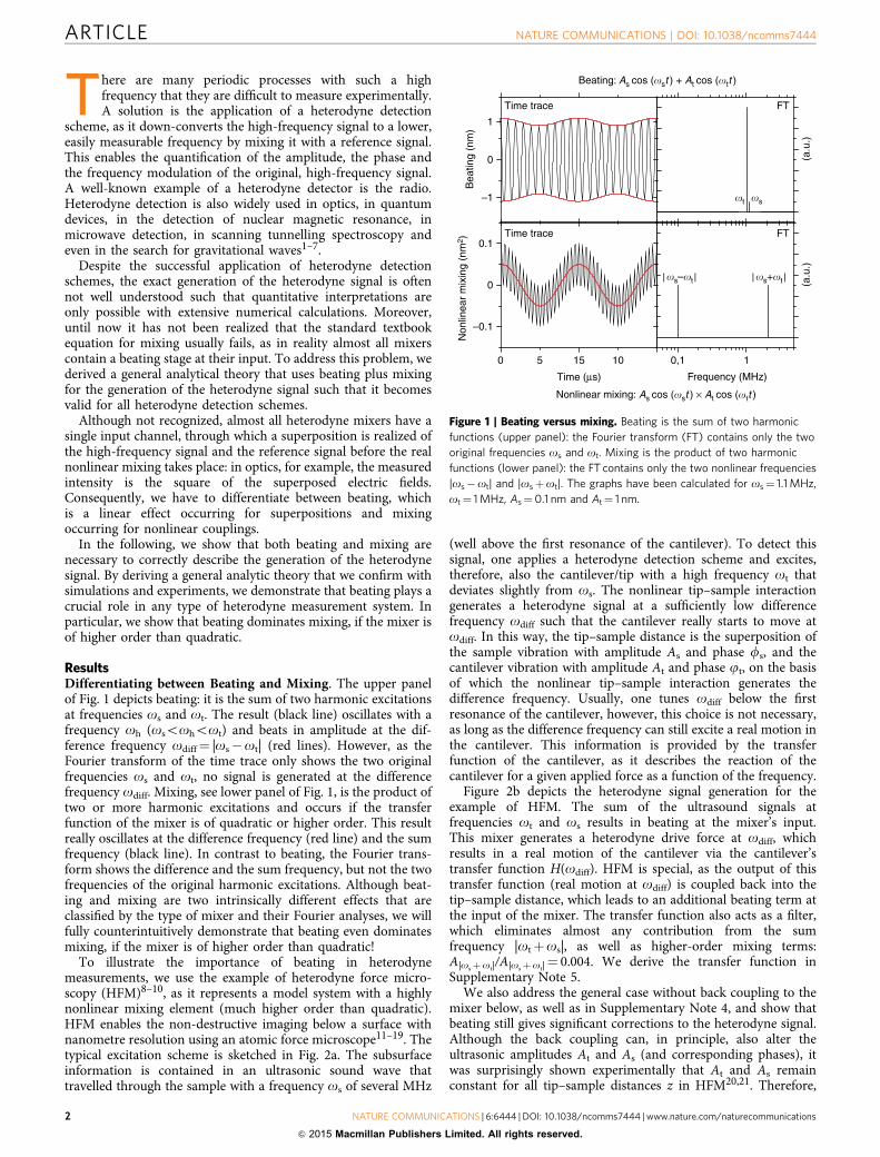
Figure 2 | Heterodyne force microscopy excitation scheme. (a) The Si sample vibrates with amplitude As and phase js at a frequency os, while the tip

vibrates with At and jt at ot. Using an optical beam method and a lock-in, we detected the amplitude Adiff and phase jdiff of the difference frequency

odiff¼ |os�ot|. The tip–sample distance z was varied by moving the cantilever towards the surface (approach) and out again (retract). (b) The tip–sample

distance is the sum of the ultrasonic motion of the cantilever At cos(ott) and the sample As cos(ost), which results in beating. The nonlinear tip–sample

interaction generates drive forces (among others at the difference frequency), which lead, via the transfer function H(odiff) of the cantilever that also acts

as a low-pass filter, to a real motion that is coupled back into the tip–sample distance (red arrow). (c) The tip–sample interaction as a function of the

distance z (left panel): obtained from the experiment (red), as used in the analytical calculation (dashed black), and a second-order approximation around

ze¼0.53 (blue). The derivative of the tip–sample interaction as a function of the distance z (right panel): as used in the analytical calculation (dashed

black) and the second-order approximation around ze¼0.53 (blue). The blue line is only a good approximation of Fts near z¼ ze¼0.53.

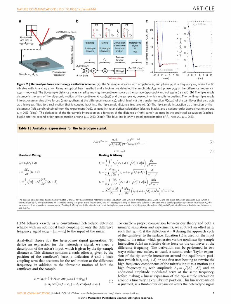
Table 1 | Analytical expressions for the heterodyne signal.

Adiffeijdiff ¼ AsAtffiffiffiffiffiffiffiffiffiffiffiffiffiffiffiffi

A2s þA2

t

p I2ei js �jtð Þ

H� 1 odiffð Þj jeiL� I1ð2Þ

d ¼ I0=k ð3ÞStandard Mixing Beating & Mixing

I0¼ Fts(zbþ d) I0 ¼1

p

Z 1

� 1Fts zbþ dþ

ffiffiffiffiffiffiffiffiffiffiffiffiffiffiffiffiA2

s þA2t

qu

� �duffiffiffiffiffiffiffiffiffiffiffiffi

1� u2p

I1 ¼@Fts

@zzbþ dð Þ I1 ¼

1

p

Z 1

� 1

@Fts

@zzbþ dþ

ffiffiffiffiffiffiffiffiffiffiffiffiffiffiffiffiA2

s þA2t

qu

� �duffiffiffiffiffiffiffiffiffiffiffiffi

1� u2p

I2 ¼1

2

ffiffiffiffiffiffiffiffiffiffiffiffiffiffiffiffiA2

s þA2t

q@2Fts

@z2zb þ dð Þ I2 ¼

1

p

Z 1

� 1

@Fts

@zzb þ dþ

ffiffiffiffiffiffiffiffiffiffiffiffiffiffiffiffiA2

s þA2t

qu

� �uduffiffiffiffiffiffiffiffiffiffiffiffi1� u2p

¼ffiffiffiffiffiffiffiffiffiffiffiffiffiffiffiffiA2

s þA2t

p2p

Z 1

� 1

@2Fts

@z2zbþ dþ

ffiffiffiffiffiffiffiffiffiffiffiffiffiffiffiffiA2

s þA2t

qu

� � ffiffiffiffiffiffiffiffiffiffiffiffi1� u2p

du

The general solutions (see Supplementary Notes 2 and 3) for the generated heterodyne signal (equation (2)), which is characterized by I1 and I2, and the static deflection (equation (3)), which ischaracterized by I0. The parameters for ‘Standard Mixing’ are given in the first column, and for ‘Beating & Mixing’ in the second column. If one assumes a purely quadratic tip–sample interaction Fts, theparameters of both solutions become equal. ‘Beating & Mixing’ explicitly takes into account the high-frequency motion and, therefore, the values of Fts and @Fts/@z at all tip–sample distances between ze

and ze±Ah.

NATURE COMMUNICATIONS | DOI: 10.1038/ncomms7444 ARTICLE

NATURE COMMUNICATIONS | 6:6444 | DOI: 10.1038/ncomms7444 | www.nature.com/naturecommunications 3

& 2015 Macmillan Publishers Limited. All rights reserved.

at most by 4.5%. The first method, referred to as ‘StandardMixing’ can be found in most textbooks, but (commonly notmentioned) this solution is valid only for second-order (quad-ratic) interactions. In contrast, our alternative approach, whichwe call ‘Beating & Mixing’, is valid for any type of interaction.The derivations and validities of both methods are described indetail in Supplementary Notes 2–4. ‘Beating & Mixing’ is a gen-eralization of the standard theory and produces the ‘StandardMixing’ results, if one artificially sets the beating term to zero. Wefind proof for our ‘Beating & Mixing’ description from excellentagreements of our results from numerical simulations and HFMexperiments, as discussed below.

Let us now compare the ‘Standard Mixing’ textbook solutionwith our ‘Beating & Mixing’ generalization, in which theamplitude Adiff and the phase jdiff of the heterodyne signal(Table 1; equation (2)) and the static deflection d of the cantilever(Table 1; equation (3)) are determined by three parameters: I0

denotes the average tip–sample interaction, I1 denotes an effectivetip–sample spring and I2 represents the nonlinear characteristics(curvature) of the mixer. In the ‘Standard Mixing’ solution, I1 andI2 are determined by the values of the first and the secondderivative of the tip–sample interaction at the equilibriumposition ze. In contrast, the ‘Beating & Mixing’ solution takesexplicitly into account the high-frequency motion and, therefore,the derivative of the tip–sample interaction at all tip–sampledistances between ze and ze±Ah. This description holds as long asAs �At is smaller than Ah

2. The three parameters I0, I1 and I2

become weighted integrals of Fts and @Fts/@z. Only if the mixer ispurely quadratic, the integrals reduce to the exact values for I0, I1

and I2 of the textbook solution of ‘Standard Mixing’ (seeSupplementary Note 3). Consequently, the ‘Beating & Mixing’solution is required for all mixers that cannot be approximatedwith a quadratic function.

The tip–sample interaction in HFM deviates significantly froma quadratic behaviour. This becomes evident from the left panelof Fig. 2c, in which we show Fts obtained from the experiment(red), Fts as used in the analytical calculation (dashed black) andthe quadratic interaction or second-order approximation of Fts

around z¼ ze¼ 0.53 nm (blue). Although the quadratic interac-tion is a good approximation of the tip–sample interaction closeto ze¼ 0.53 nm, this approximation clearly fails 1 nm further at atip–sample distance of, for example, z¼ ze¼ 1.53 nm. This is evenworse for the first derivative of the tip–sample interaction, whichis shown in the right panel of Fig. 2c. Therefore, ‘StandardMixing’ cannot describe the heterodyne signal generation inHFM: the tip–sample interaction cannot be approximatedquadratically over a z range that is equal to the typical ultrasonicvibration amplitude Ah of 1 nm.

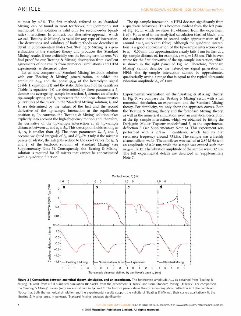
Experimental verification of the ‘Beating & Mixing’ theory.In Fig. 3, we compare the ‘Beating & Mixing’ result with a fullnumerical simulation, an experiment, and the ‘Standard Mixing’theory. For simplicity, we only show the approach curves. Boththe ‘Beating & Mixing’ theory and the ‘Standard Mixing’ theory,as well as the numerical simulation, need an analytical descriptionof the tip–sample interaction, which we obtained by fitting theDerjaguin–Muller–Toporov model22 and I0 to the experimentaldeflection d (see Supplementary Note 6). This experiment wasperformed with a 2 N m� 1 cantilever, which had its firstresonance frequency around 73 kHz. The sample was a freshlycleaned silicon wafer. The cantilever was excited at 2.87 MHz withan amplitude of 0.96 nm, while the sample was excited such thatodiff¼ 1 kHz. The vibration amplitude of the sample was 0.32 nm.The full experimental details are described in SupplementaryNote 7.

–1.5

–1.0

–0.5

0.0

0.5

1.0

Can

tilev

er d

efle

ctio

n, �

(nm

)

1E–3

0.01

0.1

1

10

ExperimentNumerical simulation

Tip–sample distance, defined by cantilever's base zb (nm)

–1 0 1 2 3 0 1 2 3 0 1 2 3 0 1 2 3–1 –1 –1

Contact force, Fc (nN)

0 0 0 01.6 1.6 1.6 1.6

Het

erod

yne

sign

al, A

diff

(nm

)

Beating & Mixing Standard Mixing

Figure 3 | Comparison between analytical theory, simulation, and an experiment. The heterodyne amplitude Adiff as obtained from ‘Beating &

Mixing’ (a: red), from a full numerical simulation (b: black), from the experiment (c: black) and from ‘Standard Mixing’ (d: black). For comparison,

the ‘Beating & Mixing’ curves (red) are also shown in b,c and d. The bottom panels show the corresponding static deflection d of the cantilever.

Notice that both the numerical simulation and the experimental results support the validity of ‘Beating & Mixing’: their curves qualitatively fit the

‘Beating & Mixing’ ones. In contrast, ‘Standard Mixing’ deviates significantly.

ARTICLE NATURE COMMUNICATIONS | DOI: 10.1038/ncomms7444

4 NATURE COMMUNICATIONS | 6:6444 | DOI: 10.1038/ncomms7444 | www.nature.com/naturecommunications

& 2015 Macmillan Publishers Limited. All rights reserved.

To confirm that ‘Beating & Mixing’ is important in HFM, wecalculated both the amplitude of the heterodyne signal Adiff andthe deflection d as a function of the tip–sample distance (definedby the cantilever’s base position zb; see Fig. 3a). The numericalsimulations quantitatively fit our ‘Beating & Mixing’ curves (seeblack line in Fig. 3b) perfectly. Additional proof comes also fromexperiments (see Fig. 3c)21, as the general curvature correctlyreproduces the ‘Beating & Mixing’ results at all tip–sampledistances zb. If we compare the textbook solution of ‘StandardMixing’ shown in Fig. 3d, one clearly notices a significantdeviation: ‘Standard Mixing’ fails to describe the mixing signal.This is in contradiction with the general conception that standardfrequency mixing generates the observed signal in HFM.The discontinuities, in both the amplitude and the deflection,are due to the specific choice of tip–sample interaction (seeSupplementary Note 6). In conclusion, this confirms that ‘Beating& Mixing’ indeed correctly describes the generation the differencesignal in HFM and that ‘Standard Mixing’ fails.

DiscussionLet us now discuss the significant effect of the ultrasound on thedeflection in HFM, which can be evaluated by the static output(I0) of the mixer with respect to the case without ultrasound.Alternatively, one can compare the deflection curves of the‘Standard Mixing’ theory with the ‘Beating & Mixing’ theory,which is shown in Fig. 3d. In conclusion, both the adhesion andthe elasticity appear smaller in HFM experiments, if one does notaccount for the existence of the ultrasound.

Finally, we address the more general case of heterodynemeasurements without a back coupling to the input of the mixeras existent in HFM. Even without back coupling, beating is stillessential to correctly describe the heterodyne signal generation.As the back coupling term in HFM is generated by I1 (seeSupplementary Note 4), we can set I1 to zero in equation (2). Alsowithout back coupling, ‘Beating & Mixing’ still determines theheterodyne signal and the static deflection through the para-meters I0 and I2. Therefore, we generally conclude that beating isof crucial importance for heterodyne detection schemes.

In conclusion, we have shown that beating, although it is alinear effect and has never considered to be of importance inheterodyne detection schemes, dominates the generation of thesignal at the difference frequency in heterodyne measurements.We derived a general, analytical theory for any type of interactionthat takes into account Beating & Mixing, and shown that our‘Beating & Mixing’ theory correctly produces the standardbeating solution for a pure linear interaction, as well as theStandard Mixing solution for an interaction that is purelyquadratic. Correction terms are necessary for any interaction thatis of higher order than quadratic. We verified our theory with afinite time step simulation and with an experiment applyingHFM, which is a typical example of a heterodyne measurementwith a highly non-quadratic mixer.

References1. Pfeifer, T. et al. Heterodyne mixing of laser fields for temporal gating of high-

order harmonic generation. Phys. Rev. Lett. 97, 163901 (2006).2. Berciaud, S., Cognet, L., Blab, G. A. & Lounis, B. Photothermal heterodyne

imaging of individual nonfluorescent nanoclusters and nanocrystals. Phys. Rev.Lett. 93, 257402 (2004).

3. Turchette, Q. A., Hood, C. J., Lange, W., Mabucchi, H. & Kimble, H. J.Measurement of conditional phase shifts for quantum logic. Phys. Rev. Lett. 75,254710 (1995).

4. Mlynek, J., Wong, N. C., DeVoe, R. G., Kintzer, E. S. & Brewer, R. G. Ramanheterodyne detection of nuclear magnetic resonance. Phys. Rev. Lett. 50,130993 (1983).

5. Diddams, S. A. et al. Direct link between microwave and optical frequencieswith a 300 THz femtosecond laser comb. Phys. Rev. Lett. 84, 225102 (2000).

6. Matsuyama, E. et al. Principles and application of heterodyne scanningtunnelling spectroscopy. Sci. Rep. 4, 6711 (2014).

7. Thorne, K. S. Gravitational-wave research: current status and future prospects.Rev. Mod. Phys. 52, 020285 (1980).

8. Kolosov, O. & Yamanaka, K. Nonlinear detection of ultrasonic vibrations in anatomic force microscope. Jpn J. Appl. Phys. 32, 8AL1095 (1993).

9. Yamanaka, K. & Nakano, S. Ultrasonic atomic force microscope with overtoneexcitation of cantilever. Jpn J. Appl. Phys. 35, 6B3787 (1996).

10. Cuberes, M. T., Assender, H. E., Briggs, G. A. D. & Kolosov, O. V. Heterodyneforce microscopy of PMMA/rubber nanocomposites: nanomapping ofviscoelastic response at ultrasonic frequencies. J. Appl. Phys. D 33, 192347(2000).

11. Shekhawat, G. S. & Dravid, V. P. Nanoscale imaging of buried structures viascanning near-field ultrasound holography. Science 310, 574589 (2005).

12. Cantrell, S. A., Cantrell, J. H. & Lillehei, P. T. Nanoscale subsurface imaging viaresonant difference-frequency atomic force ultrasonic microscopy. J. Appl.Phys. 101, 114324 (2007).

13. Cuberes, M. T. Intermittent-contact heterodyne force microscopy.J. Nanomater. 2009, 762016 (2009).

14. Shekhawat, G. S., Srivastava, A., Avasthy, S. & Dravid, V. P. Ultrasoundholography for noninvasive imaging of buried defects and interfaces foradvanced interconnect architectures. Appl. Phys. Lett. 95, 263101 (2009).

15. Tetard, L. et al. Elastic phase response of silica nanoparticles buried in softmatter. Appl. Phys. Lett. 93, 133113 (2008).

16. Tetard, L. et al. Spectroscopy and atomic force microscopy of biomass.Ultramicroscopy 110, 701–707 (2010).

17. Tetard, L., Passian, A., Farahi, R. H. & Thundat, T. Atomic force microscopy ofsilica nanoparticles and carbon nanohorns in macrophages and red blood cells.Ultramicroscopy 110, 586–591 (2010).

18. Tetard, L., Passian, A. & Thundat, T. New modes for subsurface atomic forcemicroscopy through nanomechanical coupling. Nat. Nanotechnol. 5, 105–109(2010).

19. Tetard, L. et al. Imaging nanoparticles in cells by nanomechanical holography.Nat. Nanotechnol. 3, 501–505 (2008).

20. Verbiest, G. J., Oosterkamp, T. H. & Rost, M. J. Cantilever dynamics inheterodyne force microscopy. Ultramicroscopy 135, 113–120 (2013).

21. Verbiest, G. J., Oosterkamp, T. H. & Rost, M. J. Subsurface-AFM: sensitivity tothe heterodyne signal. Nanotechnology 24, 365701 (2013).

22. Dejarguin, B. V., Muller, V. M. & Toporov, Y. P. Effect of contact deformationson the adhesion of particles. J. Colloid Interf. Sci. 53, 314–326 (1975).

AcknowledgementsThe research described in this paper has been performed under and financed by theNIMIC (http://www.realnano.nl) consortium under project 4.4. We acknowledge J.M. deVoogd, B. van Waarde and J.J.T. Wagenaar for proofreading of the manuscript.

Author contributionsM.J.R. realized the problem with beating. G.J.V. proposed the analytical model, workedout the equations and performed the experiments, as well as the simulations. Bothauthors discussed and interpreted the results, and also wrote the manuscript together.The project was initiated and conceptualized by M.J.R.

Additional informationSupplementary Information accompanies this paper at http://www.nature.com/naturecommunications

Competing financial interests: The authors declare no competing financial interest.

Reprints and permission information is available online at http://npg.nature.com/reprintsandpermissions/

How to cite this article: Verbiest, G. J. and Rost, M. J. Beating beats mixing inheterodyne detection schemes. Nat. Commun. 6:6444 doi: 10.1038/ncomms7444 (2015).

NATURE COMMUNICATIONS | DOI: 10.1038/ncomms7444 ARTICLE

NATURE COMMUNICATIONS | 6:6444 | DOI: 10.1038/ncomms7444 | www.nature.com/naturecommunications 5

& 2015 Macmillan Publishers Limited. All rights reserved.

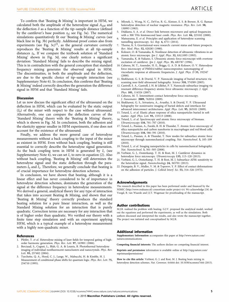
Supplementary Figure 1 | Force versus distance curves from measurements with a hard Silicon

tip/cantilever pushing into a hard Silicon wafer: obtained from the experiment (red) and as used in the

analytical calculation (dashed black). Please note that Fts(z = 0) ≠ 0 per definition.

r

0 1.87441 73.4 kHz

1 4.67949 456 kHz

2 7.78852 1.27 MHz

3 10.8007 2.44 MHz

4 13.6737 3.91 MHz

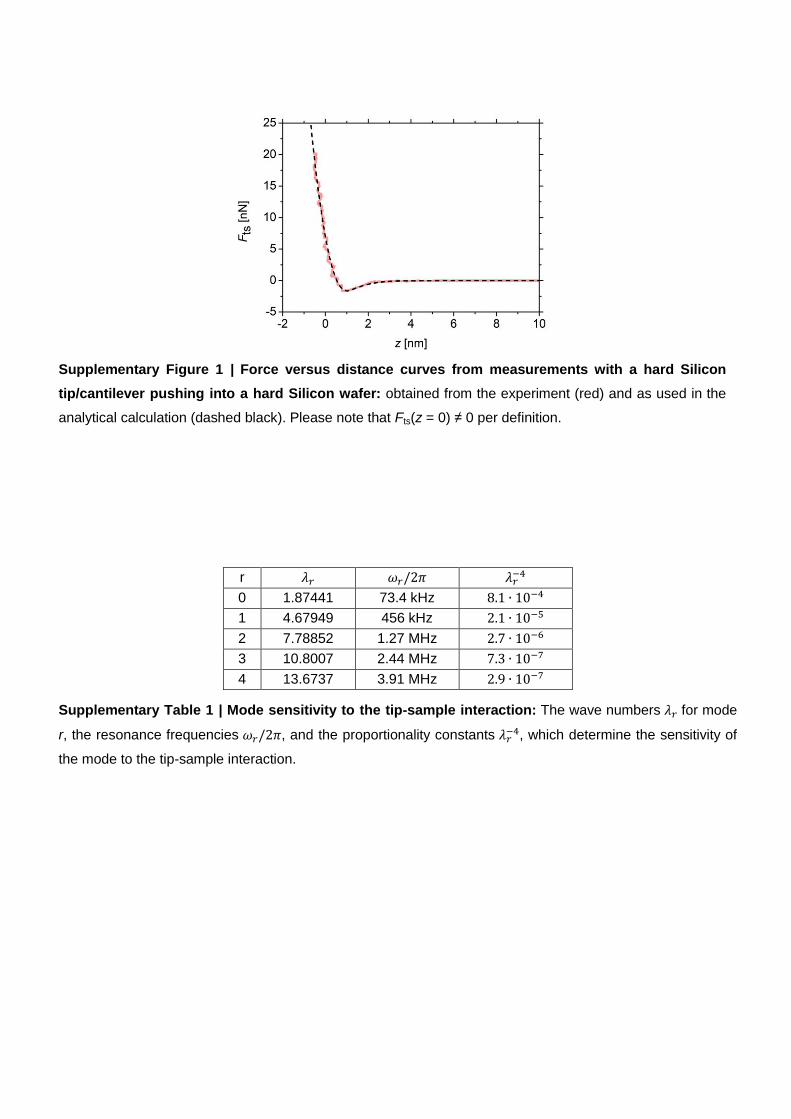
Supplementary Table 1 | Mode sensitivity to the tip-sample interaction: The wave numbers for mode

r, the resonance frequencies , and the proportionality constants , which determine the sensitivity of

the mode to the tip-sample interaction.

SUPPLEMENTARY NOTE 1 - INTRODUCTION

In the Supplementary Notes we discuss both the analytical methods and the experimental details that are

needed to understand the dynamics in Heterodyne Force Microscopy (HFM), which is a nonlinear mechanical

system driven simultaneously at two different frequencies.

In Supplementary Note 2 we derive analytical equations for the difference frequency generation considering

only standard nonlinear mixing, and a combination of beating and mixing in Supplementary Note 3. Both

solutions show that a nonlinear tip-sample interaction is required to produce a signal at the difference

frequency. We also show that both solutions are equal as long as the tip-sample interaction is purely

quadratic. However, the solutions differ significantly, if the interaction is more nonlinear than purely quadratic,

which is the case in HFM. The standard solution of mixing fails and, instead, one has to consider a

combination of beating and mixing. The main essence is that the high frequency beating motion leads to two

correction terms that alter the standard solution.

In HFM the nonlinear tip-sample interaction generates a force at the difference frequency, which leads to a

feedback on the tip-sample distance, as the cantilever really vibrates at the difference frequency. As a

feedback mechanism is usually absent in standard nonlinear mixing, we discuss the solutions without

feedback in Supplementary Note 4 and obtain that beating still produces a correction term to the amplitude

and the phase of the difference frequency in comparison to the standard solutions.

To evaluate the analytical solutions as a function of the tip-sample distance such that we can compare

them with the difference frequency generation results from experiments, we need the inverse transfer function

of the cantilever at the difference frequency, an expression for the tip-sample interaction, and the amplitudes

As and At of the ultrasonic excitations of the sample and the cantilever respectively.

In Supplementary Note 5 we derive an analytical equation for the inverse transfer function of the cantilever

by making a mode expansion. To enable a correct comparison, we use values in the final description that

match our experimental values as close as possible. In Supplementary Note 6 we fit an experimentally

measured tip-sample interaction to obtain a realistic, analytical expression for it. Finally, we describe our

experimental details in Supplementary Note 7, in which we also explain how we determine the amplitudes As

and At of the ultrasonic excitations.

SUPPLEMENTARY NOTE 2 - DIFFERENCE FREQUENCY GENERATION CONSIDERING NONLINEAR MIXING ONLY

In this Supplementary Note we provide the equations for standard nonlinear mixing as they are derived

normally using a second order Taylor expansion. We start with an equation for the tip-sample distance z. This

distance has a static offset zb, which is given by the height of the base of the cantilever. In addition, we have

to take into account a possible bending of the cantilever, which results in a change of z and is described by

the deflection δ. Furthermore, the tip-sample distance z contains the ultrasonic motion of both the cantilever

at frequency ωt and the sample at frequency ωs. Finally, we have to add a feedback term that accounts for a

variation of z at the difference frequency ωdiff = |ωs − ωt|, as the cantilever really vibrates at ωdi due to the

effect of the nonlinear tip-sample interaction. If H(ωdiff) denotes the transfer function of the cantilever that

transfers a given force into an amplitude, the feedback term is given by H(ωdiff)F(ωdiff), in which F(ωdiff)

describes the drive force on the cantilever at the difference frequency ωdiff. To keep our description as general

as possible, we do not make any assumptions on the drive force F(ωdiff), and we evaluate F(ωdiff) from the

motion of the cantilever at the difference frequency such that F(ωdiff) = Adiff|H−1

(ωdiff)| cos(ωdifft + φdiff + 𝛬), in

which |H−1

(ωdiff)| denotes the absolute value of the inverse transfer function of the cantilever and 𝛬 denotes

the corresponding phase shift. Therefore, the feedback term is simply given by Adiff cos(ωdifft + φdiff). This

leads to the following equation for the tip-sample distance:

( ) ( ) ( ) (1)

We use the derived expression for the tip-sample distance, Eq. 1, in the tip-sample interaction Fts(z) to find

the effective drive force on the cantilever at the difference frequency. To take into account nonlinear mixing,

we approximate the tip-sample interaction Fts(z) by a conventional second order Taylor expansion. Higher

order terms are usually neglected, as their values are sufficiently small. The square term will produce a

nonlinear mixing term. Since we use a second order Taylor expansion that we evaluate in a fixed, single

point, it is to be expected that the description holds exactly only for quadratic interactions.

( ( ) ( ) ( )) (2)

( )

( )[ ( ) ( ) ( )]

( )[ ( ) ( ) ( )]

As the high frequency motion of the cantilever is unaltered1, and as we are only interested in the static

deflection of the cantilever and its motion at the difference frequency ωdiff, we evaluate Eq. 2 further and

collect only the terms at zero frequency and the difference frequency ωdiff. For the evaluation of the square

term, we make use of ( ) ( ) [ ( ) ( )] such that e.g. [ (

)]

( ) and ( ) ( ) (

[ ]) ([ ] [ ]) . Keeping only the terms at zero frequency and at

frequency ωdiff, we find the following equation of motion

( )

( ) ( )

( ) [

( [ ])⏟

]

| ( )| ( 𝛬) (3)

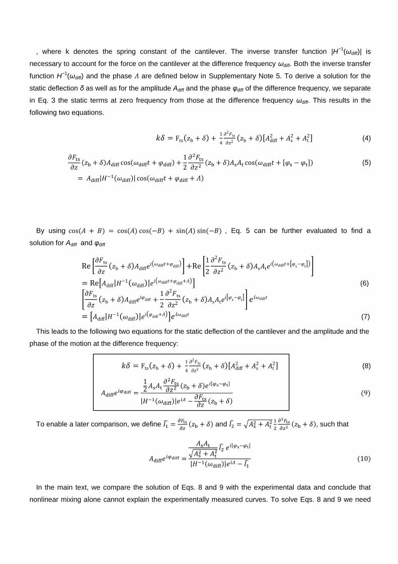
, where k denotes the spring constant of the cantilever. The inverse transfer function |H−1

(ωdiff)| is

necessary to account for the force on the cantilever at the difference frequency ωdiff. Both the inverse transfer

function H−1

(ωdiff) and the phase 𝛬 are defined below in Supplementary Note 5. To derive a solution for the

static deflection δ as well as for the amplitude Adiff and the phase φdiff of the difference frequency, we separate

in Eq. 3 the static terms at zero frequency from those at the difference frequency ωdiff. This results in the

following two equations.

( )

( )[

] (4)

( ) ( )

( ) ( [ ])

| ( )| ( 𝛬)

By using ( ) ( ) ( ) ( ) ( ) , Eq. 5 can be further evaluated to find a

solution for Adiff and φdiff

[

( )

( )] [

( )

( [ ])]

[ | ( )|

( 𝛬)] (6)

[

( )

( )

[ ]]

[ | ( )|

( 𝛬)] (7)

This leads to the following two equations for the static deflection of the cantilever and the amplitude and the

phase of the motion at the difference frequency:

( )

( )[

] (8)

( ) [ ]

| ( )|

( ) ( )

To enable a later comparison, we define

( ) and √

( ), such that

√

[ ]

| ( )| ( )

In the main text, we compare the solution of Eqs. 8 and 9 with the experimental data and conclude that

nonlinear mixing alone cannot explain the experimentally measured curves. To solve Eqs. 8 and 9 we need

the inverse transfer function of the cantilever H−1

(ωdiff) (see Supplementary Note 5), the tip-sample interaction

Fts(z) (see Supplementary Note 6), and the amplitudes At and As of the ultrasonic vibrations (see

Supplementary Note 7).

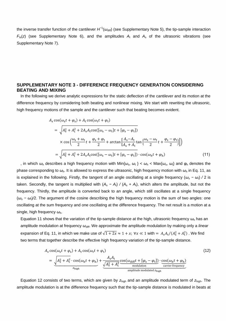
SUPPLEMENTARY NOTE 3 - DIFFERENCE FREQUENCY GENERATION CONSIDERING BEATING AND MIXING

In the following we derive analytic expressions for the static deflection of the cantilever and its motion at the

difference frequency by considering both beating and nonlinear mixing. We start with rewriting the ultrasonic,

high frequency motions of the sample and the cantilever such that beating becomes evident.

( ) ( )

√ ([ ] [ ])

(

[

{

}])

√ ([ ] [ ]) ( )

, in which ωh describes a high frequency motion with Min{ωs, ωt } < ωh < Max{ωs, ωt} and φh denotes the

phase corresponding to ωh. It is allowed to express the ultrasonic, high frequency motion with ωh in Eq. 11, as

is explained in the following. Firstly, the tangent of an angle oscillating at a single frequency (ωs − ωt) / 2 is

taken. Secondly, the tangent is multiplied with (As − At) / (As + At), which alters the amplitude, but not the

frequency. Thirdly, the amplitude is converted back to an angle, which still oscillates at a single frequency

(ωs − ωt)/2. The argument of the cosine describing the high frequency motion is the sum of two angles: one

oscillating at the sum frequency and one oscillating at the difference frequency. The net result is a motion at a

single, high frequency ωh.

Equation 11 shows that the variation of the tip-sample distance at the high, ultrasonic frequency ωh has an

amplitude modulation at frequency ωdiff. We approximate the amplitude modulation by making only a linear

expansion of Eq. 11, in which we make use of √ with (

)⁄ . We find

two terms that together describe the effective high frequency variation of the tip-sample distance.

( ) ( ) (12)

√ ( )⏟

√ ( [ ])⏟

( )⏟ ⏟

Equation 12 consists of two terms, which are given by zhigh and an amplitude modulated term of zhigh. The

amplitude modulation is at the difference frequency such that the tip-sample distance is modulated in beats at

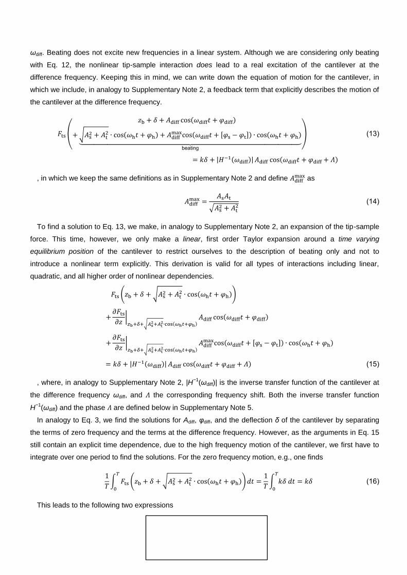
ωdiff. Beating does not excite new frequencies in a linear system. Although we are considering only beating

with Eq. 12, the nonlinear tip-sample interaction does lead to a real excitation of the cantilever at the

difference frequency. Keeping this in mind, we can write down the equation of motion for the cantilever, in

which we include, in analogy to Supplementary Note 2, a feedback term that explicitly describes the motion of

the cantilever at the difference frequency.

(

( )

√

( ) ( [ ]) ( )⏟

)

| ( )| ( 𝛬)

, in which we keep the same definitions as in Supplementary Note 2 and define as

√

To find a solution to Eq. 13, we make, in analogy to Supplementary Note 2, an expansion of the tip-sample

force. This time, however, we only make a linear, first order Taylor expansion around a time varying

equilibrium position of the cantilever to restrict ourselves to the description of beating only and not to

introduce a nonlinear term explicitly. This derivation is valid for all types of interactions including linear,

quadratic, and all higher order of nonlinear dependencies.

( √ ( ))

| √

( )

( )

| √

( )

( [ ]) ( )

| ( )| ( 𝛬)

, where, in analogy to Supplementary Note 2, |H−1

(ωdiff)| is the inverse transfer function of the cantilever at

the difference frequency ωdiff, and 𝛬 the corresponding frequency shift. Both the inverse transfer function

H−1

(ωdiff) and the phase 𝛬 are defined below in Supplementary Note 5.

In analogy to Eq. 3, we find the solutions for Adiff, φdiff, and the deflection δ of the cantilever by separating

the terms of zero frequency and the terms at the difference frequency. However, as the arguments in Eq. 15

still contain an explicit time dependence, due to the high frequency motion of the cantilever, we first have to

integrate over one period to find the solutions. For the zero frequency motion, e.g., one finds

∫ ( √

( ))

∫

This leads to the following two expressions

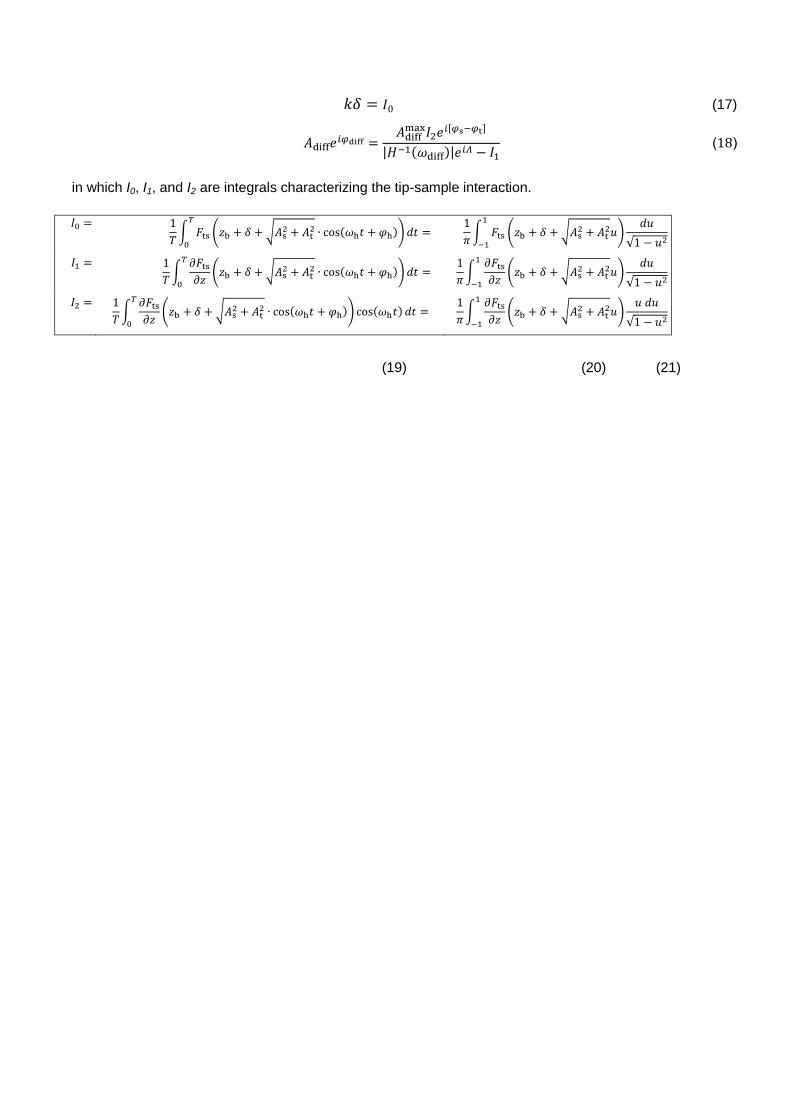
(17)

[ ]

| ( )|

in which I0, I1, and I2 are integrals characterizing the tip-sample interaction.

∫ ( √

( ))

∫ ( √

)

√

∫

( √

( ))

∫

( √

)

√

∫

( √

( )) ( )

∫

( √

)

√

(19) v (20) (21)

The integrals over the parameter u (right hand side) in equations 19 ,20, and 21 are obtained by using an

Abel transform of the integrals over time T = 2π/ωh. As we integrate over one period T, the integrals become

independent of φh and we can set the phase φh to 0.

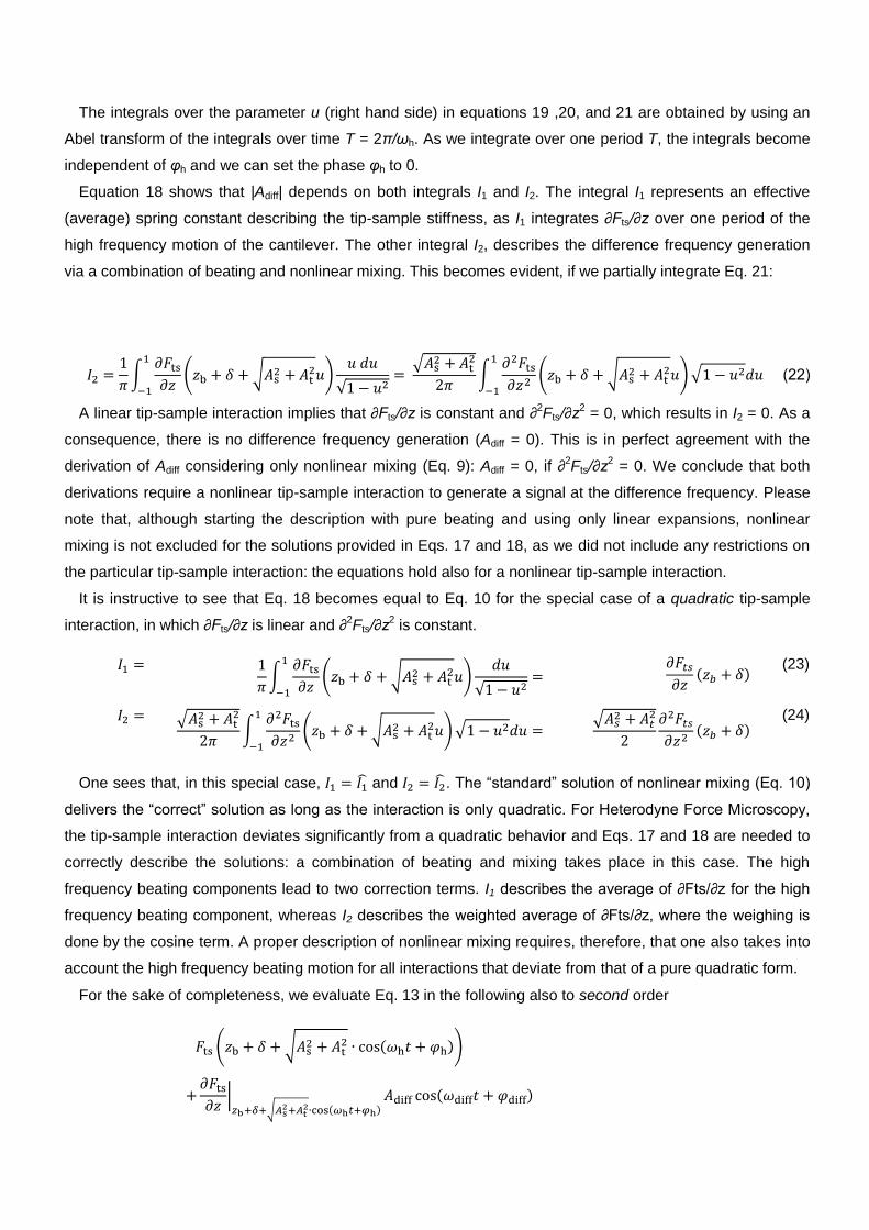
Equation 18 shows that |Adiff| depends on both integrals I1 and I2. The integral I1 represents an effective

(average) spring constant describing the tip-sample stiffness, as I1 integrates ∂Fts/∂z over one period of the

high frequency motion of the cantilever. The other integral I2, describes the difference frequency generation

via a combination of beating and nonlinear mixing. This becomes evident, if we partially integrate Eq. 21:

∫

( √ )

√

√

∫

( √ )√

A linear tip-sample interaction implies that ∂Fts/∂z is constant and ∂2Fts/∂z

2 = 0, which results in I2 = 0. As a

consequence, there is no difference frequency generation (Adiff = 0). This is in perfect agreement with the

derivation of Adiff considering only nonlinear mixing (Eq. 9): Adiff = 0, if ∂2Fts/∂z

2 = 0. We conclude that both

derivations require a nonlinear tip-sample interaction to generate a signal at the difference frequency. Please

note that, although starting the description with pure beating and using only linear expansions, nonlinear

mixing is not excluded for the solutions provided in Eqs. 17 and 18, as we did not include any restrictions on

the particular tip-sample interaction: the equations hold also for a nonlinear tip-sample interaction.

It is instructive to see that Eq. 18 becomes equal to Eq. 10 for the special case of a quadratic tip-sample

interaction, in which ∂Fts/∂z is linear and ∂2Fts/∂z

2 is constant.

∫

( √ )

√

( ) (23)

√

∫

( √ )√

√

( ) (24)

One sees that, in this special case, and . Th “s d rd” solu o of o l r m x Eq. 0

d l v rs h “corr c ” solu o s lo s h r c o s o ly qu dr c. For H rody Forc M croscopy,

the tip-sample interaction deviates significantly from a quadratic behavior and Eqs. 17 and 18 are needed to

correctly describe the solutions: a combination of beating and mixing takes place in this case. The high

frequency beating components lead to two correction terms. I1 d scr s h v r of ∂F s/∂z for h h h

frequency beating component, whereas I2 d scr s h w h d v r of ∂F s/∂z, wh r h w h s

done by the cosine term. A proper description of nonlinear mixing requires, therefore, that one also takes into

account the high frequency beating motion for all interactions that deviate from that of a pure quadratic form.

For the sake of completeness, we evaluate Eq. 13 in the following also to second order

( √ ( ))

| √

( )

( )

| √

( )

( [ ]) ( )

| √

( )

[

( ) ( )

([ ] ) ( )

]

| ( )| ( 𝛬)

By separating the components with zero frequency and the difference frequency, we find the following

solutions:

([ ] )

(

) (26)

[ ]

| ( )|

, in which the terms I0, I1, and I2 are given by Eqs. 19, 20, and 21, and

∫

( √

( ))

∫

( √

)

√

(28)

∫

( √

( )) ( )

∫

( √

)

√

(29)

∫

( √

( )) ( )

∫

( √

)

√

(30)

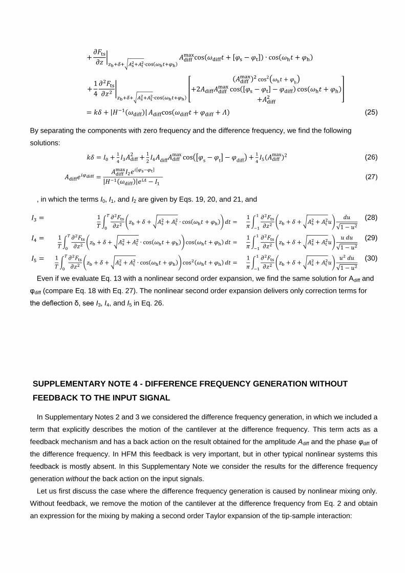
Even if we evaluate Eq. 13 with a nonlinear second order expansion, we find the same solution for Adiff and

φdiff (compare Eq. 18 with Eq. 27). The nonlinear second order expansion delivers only correction terms for

h d fl c o δ, s I3, I4, and I5 in Eq. 26.

SUPPLEMENTARY NOTE 4 - DIFFERENCE FREQUENCY GENERATION WITHOUT

FEEDBACK TO THE INPUT SIGNAL

In Supplementary Notes 2 and 3 we considered the difference frequency generation, in which we included a

term that explicitly describes the motion of the cantilever at the difference frequency. This term acts as a

feedback mechanism and has a back action on the result obtained for the amplitude Adiff and the phase φdiff of

the difference frequency. In HFM this feedback is very important, but in other typical nonlinear systems this

feedback is mostly absent. In this Supplementary Note we consider the results for the difference frequency

generation without the back action on the input signals.

Let us first discuss the case where the difference frequency generation is caused by nonlinear mixing only.

Without feedback, we remove the motion of the cantilever at the difference frequency from Eq. 2 and obtain

an expression for the mixing by making a second order Taylor expansion of the tip-sample interaction:

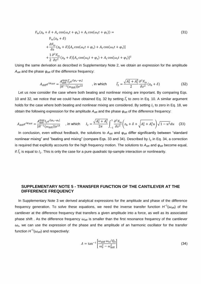
( ( ) ( )) (31)

( )

( )[ ( ) ( )]

( )[ ( ) ( )]

Using the same derivation as described in Supplementary Note 2, we obtain an expression for the amplitude

Adiff and the phase φdiff of the difference frequency:

[ ]

| ( )| , wh ch

√

( )

Let us now consider the case where both beating and nonlinear mixing are important. By comparing Eqs.

10 and 32, we notice that we could have obtained Eq. 32 by setting to zero in Eq. 10. A similar argument

holds for the case where both beating and nonlinear mixing are considered. By setting to zero in Eq. 18, we

obtain the following expression for the amplitude Adiff and the phase φdiff of the difference frequency:

[ ]

| ( )| , wh ch

√

∫

( √ )√

In conclusion, even without feedback, the solutions to Adiff and φdiff d ff r s f c ly w “s d rd

o l r m x ” d ” d m x ” comp r Eqs. d . Described by in Eq. 34, a correction

is required that explicitly accounts for the high frequency motion. The solutions to Adiff and φdiff become equal,

if is equal to . This is only the case for a pure quadratic tip-sample interaction or nonlinearity.

SUPPLEMENTARY NOTE 5 - TRANSFER FUNCTION OF THE CANTILEVER AT THE DIFFERENCE FREQUENCY

In Supplementary Note 3 we derived analytical expressions for the amplitude and phase of the difference

frequency generation. To solve these equations, we need the inverse transfer function H−1

(ωdiff) of the

cantilever at the difference frequency that transfers a given amplitude into a force, as well as its associated

phase shift . As the difference frequency ωdiff is smaller than the first resonance frequency of the cantilever

ω0, we can use the expression of the phase and the amplitude of an harmonic oscillator for the transfer

function H−1

(ωdiff) and respectively:

𝛬 [ ⁄

]

( )

( ) √(

)

(

)

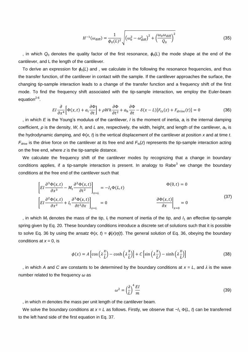
, in which Q0 denotes the quality factor of the first resonance, ϕ0(L) the mode shape at the end of the

cantilever, and L the length of the cantilever.

To derive an expression for ϕ0(L) and , we calculate in the following the resonance frequencies, and thus

the transfer function, of the cantilever in contact with the sample. If the cantilever approaches the surface, the

changing tip-sample interaction leads to a change of the transfer function and a frequency shift of the first

mode. To find the frequency shift associated with the tip-sample interaction, we employ the Euler-beam

equation2-6

.

[ ( )

]

( )[ ( ) ( )]

, in which E s h You ’s modulus of h c l v r, I is the moment of inertia, ai is the internal damping

coefficient, ρ is the density, W, h, and L are, respectively, the width, height, and length of the cantilever, ah is

the hydrodynamic damping, and (x, t) is the vertical displacement of the cantilever at position x and at time t.

Fdrive is the drive force on the cantilever at its free end and Fts(z) represents the tip-sample interaction acting

on the free end, where z is the tip-sample distance.

We calculate the frequency shift of the cantilever modes by recognizing that a change in boundary

conditions applies, if a tip-sample interaction is present. In analogy to Rabe3 we change the boundary

conditions at the free end of the cantilever such that

[ ( )

( )

]

( ) ( )

(37)

[ ( )

( )

]

( )

|

, in which Mt denotes the mass of the tip, It the moment of inertia of the tip, and I1 an effective tip-sample

spring given by Eq. 20. These boundary conditions introduce a discrete set of solutions such that it is possible

to solve Eq. 36 by using the ansatz (x, t) = ϕ(x)η(t). The general solution of Eq. 36, obeying the boundary

conditions at x = 0, is

( ) [ (

) (

)] [ (

) (

)]

, in which A and C are constants to be determined by the boundary conditions at x = L, and is the wave

number related to the frequency ω as

(

)

, in which m denotes the mass per unit length of the cantilever beam.

We solve the boundary conditions at x = L as follows. Firstly, we observe that −I1 (L, t) can be transferred

to the left hand side of the first equation in Eq. 37.

[ ( )

( )

( )]

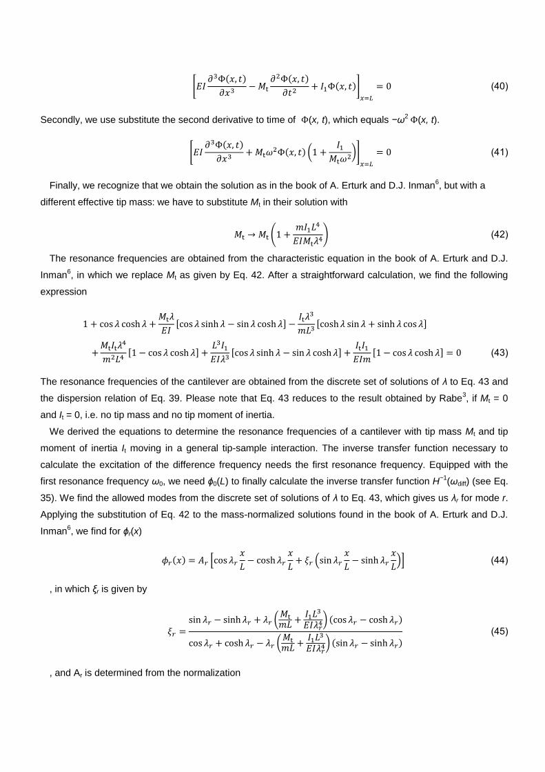
0

Secondly, we use substitute the second derivative to time of (x, t), which equals −ω2 (x, t).

[ ( )

( ) (

)]

Finally, we recognize that we obtain the solution as in the book of A. Erturk and D.J. Inman6, but with a

different effective tip mass: we have to substitute Mt in their solution with

(

)

The resonance frequencies are obtained from the characteristic equation in the book of A. Erturk and D.J.

Inman6, in which we replace Mt as given by Eq. 42. After a straightforward calculation, we find the following

expression

[ ]

[ ]

[ ]

[ ]

[ ]

The resonance frequencies of the cantilever are obtained from the discrete set of solutions of λ to Eq. 43 and

the dispersion relation of Eq. 39. Please note that Eq. 43 reduces to the result obtained by Rabe3, if Mt = 0

and It = 0, i.e. no tip mass and no tip moment of inertia.

We derived the equations to determine the resonance frequencies of a cantilever with tip mass Mt and tip

moment of inertia It moving in a general tip-sample interaction. The inverse transfer function necessary to

calculate the excitation of the difference frequency needs the first resonance frequency. Equipped with the

first resonance frequency ω0, we need ϕ0(L) to finally calculate the inverse transfer function H−1

(ωdiff) (see Eq.

35). We find the allowed modes from the discrete set of solutions of λ to Eq. 43, which gives us λr for mode r.

Applying the substitution of Eq. 42 to the mass-normalized solutions found in the book of A. Erturk and D.J.

Inman6, we find for ϕr(x)

( ) [

(

)]

, in which ξr is given by

(

) ( )

(

) ( )

, and Ar is determined from the normalization

∫ ( )

( )

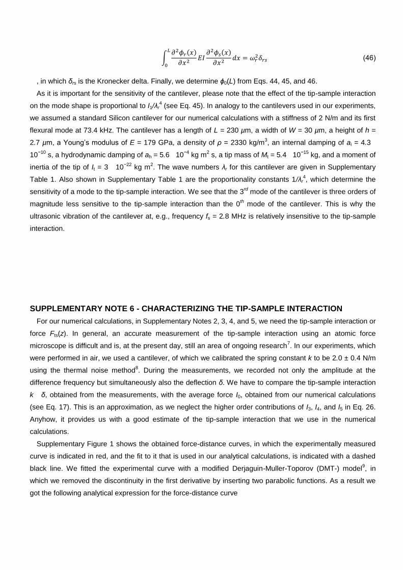
, in which δrs is the Kronecker delta. Finally, we determine ϕ0(L) from Eqs. 44, 45, and 46.

As it is important for the sensitivity of the cantilever, please note that the effect of the tip-sample interaction

on the mode shape is proportional to I1/λr4 (see Eq. 45). In analogy to the cantilevers used in our experiments,

we assumed a standard Silicon cantilever for our numerical calculations with a stiffness of 2 N/m and its first

flexural mode at 73.4 kHz. The cantilever has a length of L = 230 µm, a width of W = 30 µm, a height of h =

2.7 µm, You ’s modulus of E = 179 GPa, a density of ρ = 2330 kg/m3, an internal damping of ai = 4.3 ·

10−10

s, a hydrodynamic damping of ah = 5.6 · 10−4

kg m2 s, a tip mass of Mt = 5.4 · 10

−15 kg, and a moment of

inertia of the tip of It = 3 · 10−22

kg m2. The wave numbers λr for this cantilever are given in Supplementary

Table 1. Also shown in Supplementary Table 1 are the proportionality constants 1/λr4, which determine the

sensitivity of a mode to the tip-sample interaction. We see that the 3rd

mode of the cantilever is three orders of

magnitude less sensitive to the tip-sample interaction than the 0th mode of the cantilever. This is why the

ultrasonic vibration of the cantilever at, e.g., frequency fs = 2.8 MHz is relatively insensitive to the tip-sample

interaction.

SUPPLEMENTARY NOTE 6 - CHARACTERIZING THE TIP-SAMPLE INTERACTION

For our numerical calculations, in Supplementary Notes 2, 3, 4, and 5, we need the tip-sample interaction or

force Fts(z). In general, an accurate measurement of the tip-sample interaction using an atomic force

microscope is difficult and is, at the present day, still an area of ongoing research7. In our experiments, which

were performed in air, we used a cantilever, of which we calibrated the spring constant k to be 2.0 ± 0.4 N/m

using the thermal noise method8. During the measurements, we recorded not only the amplitude at the

difference frequency but simultaneously also the deflection δ. We have to compare the tip-sample interaction

k · δ, obtained from the measurements, with the average force I0, obtained from our numerical calculations

(see Eq. 17). This is an approximation, as we neglect the higher order contributions of I3, I4, and I5 in Eq. 26.

Anyhow, it provides us with a good estimate of the tip-sample interaction that we use in the numerical

calculations.

Supplementary Figure 1 shows the obtained force-distance curves, in which the experimentally measured

curve is indicated in red, and the fit to it that is used in our analytical calculations, is indicated with a dashed

black line. We fitted the experimental curve with a modified Derjaguin-Muller-Toporov (DMT-) model9, in

which we removed the discontinuity in the first derivative by inserting two parabolic functions. As a result we

got the following analytical expression for the force-distance curve

( )

{

√ ( )

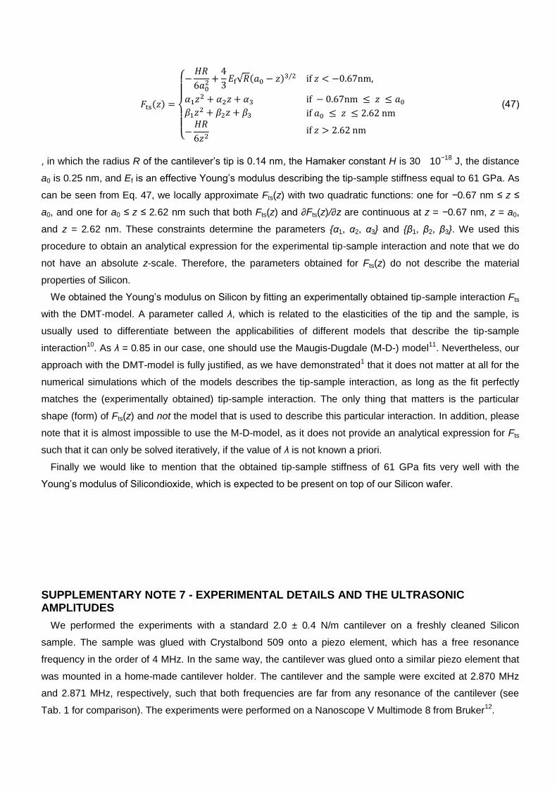
, in which the radius R of h c l v r’s p s 0. m, h H m k r co s H is 30 · 10−18

J, the distance

a0 is 0.25 nm, and Ef s ff c v You ’s modulus d scr h p-sample stiffness equal to 61 GPa. As

can be seen from Eq. 47, we locally approximate Fts(z) with two quadratic functions: one for −0.67 nm ≤ z ≤

a0, and one for a0 ≤ z ≤ 2.62 nm such that both Fts(z) and ∂Fts(z)/∂z are continuous at z = −0.67 nm, z = a0,

and z = 2.62 nm. These constraints determine the parameters {α1, α2, α3} and {β1, β2, β3}. We used this

procedure to obtain an analytical expression for the experimental tip-sample interaction and note that we do

not have an absolute z-scale. Therefore, the parameters obtained for Fts(z) do not describe the material

properties of Silicon.

W o d h You ’s modulus o S l co y f xp r m lly o d p-sample interaction Fts

with the DMT-model. A parameter called λ, which is related to the elasticities of the tip and the sample, is

usually used to differentiate between the applicabilities of different models that describe the tip-sample

interaction10

. As λ = 0.85 in our case, one should use the Maugis-Dugdale (M-D-) model11

. Nevertheless, our

approach with the DMT-model is fully justified, as we have demonstrated1 that it does not matter at all for the

numerical simulations which of the models describes the tip-sample interaction, as long as the fit perfectly

matches the (experimentally obtained) tip-sample interaction. The only thing that matters is the particular

shape (form) of Fts(z) and not the model that is used to describe this particular interaction. In addition, please

note that it is almost impossible to use the M-D-model, as it does not provide an analytical expression for Fts

such that it can only be solved iteratively, if the value of λ is not known a priori.

Finally we would like to mention that the obtained tip-sample stiffness of 61 GPa fits very well with the

You ’s modulus of S l co d ox d , wh ch s xp c d o pr s o op of our S l co w f r.

SUPPLEMENTARY NOTE 7 - EXPERIMENTAL DETAILS AND THE ULTRASONIC AMPLITUDES

We performed the experiments with a standard 2.0 ± 0.4 N/m cantilever on a freshly cleaned Silicon

sample. The sample was glued with Crystalbond 509 onto a piezo element, which has a free resonance

frequency in the order of 4 MHz. In the same way, the cantilever was glued onto a similar piezo element that

was mounted in a home-made cantilever holder. The cantilever and the sample were excited at 2.870 MHz

and 2.871 MHz, respectively, such that both frequencies are far from any resonance of the cantilever (see

Tab. 1 for comparison). The experiments were performed on a Nanoscope V Multimode 8 from Bruker12

.

We used the standard optical beam deflection method provided by this instrument to measure the motion of

the cantilever. Th slop of h mod sh p h c l v r’s fr d s proportional to the sensitivity. Since

we obtain the slopes of all higher eigenmodes of the cantilever from the numerical calculations, we estimate

the sensitivity, measured by the photodiode, for the 5th mode to be 12.6 times higher than the sensitivity for

the first mode. In this way, we obtained a sensitivity of 67.7 nm/V at 71.8 kHz and 5.4 nm/V at 2.87 MHz. This

leads to a measured amplitude At of the cantilever at 2.87 MHz of approximately 0.96 nm. We did not

measure the amplitude As of the sample vibration directly, which could be done with an interferometer.

Instead, as the plateau in the repulsive regime depends on the amplitudes of both the cantilever At and the

sample As 13

, we can estimate the sample amplitude As to be 0.32 nm in our experiments. During the

experiments we never saw the excitation ωs of h s mpl h c l v r’s mo o , wh ch w r u o h

unfavorable ratio of the cantilever stiffness and the sample stiffness at MHz frequencies1,13

.

Supplementary References

1. G.J. V r s , T.H. Oos rk mp, d M.J. Ros , “Su surf c -AFM: s s v y o h h rody s l”,

Nanotechnology 24, 365701 (2013)

2. J.H. C r ll, S.A. C r ll, “A ly c l mod l of h o l r dy m cs of c l v r p-sample surface

r c o s for v r ous cous c om c forc m croscop s”, Phys. Rev. B 77, 165409 (2008)

3. U. R , J. Tur r, W. Ar old, “A lys s of h h h-frequency response of atomic force microscope

c l v rs”, Appl. Phys. A. 66, S277-S282 (1998)

4. R.W S rk, W.M. H ckl, “Four r r sform d om c forc m croscopy: pp mod om c forc

microscopy yo d h Hook pprox m o ”, Surf. Sci. 457, 219228 (2000)

5. J.R. Loz o, R. G rc , “Th ory of ph s sp c roscopy mod l om c forc m croscopy”, Phys. Rev.

B 79, 014110 (2009)

6. A. Erturk, D.J. Inman, in Piezoelectric Energy Harvesting, (Wiley, New York, 2011), Appendix C

7. B. C pp ll , G. D l r, “Forc -d s c curv s y om c forc m croscopy”, Surf. Sci. Rep. 34, 1-104 (1999)

8. J.L. Hu r, J. B chho f r, “C l r o of om c forc m croscop ps”, Rev. Sci. Instrum. 64, 1868

(1993)

9. B.V. D j r u , V.M. Mull r, Y.P. Toporov, “Eff c of co c d form o s o h dh s o of p r cl s”,

J. Colloid Interf. Sci. 53, 314 - 326 (1975)

10. K.L. Joh so , “M ch cs of dh s o ”, Tr olo y I r o l , -418 (1998)

11. D. M u s, “Adh s o of sph r s: Th JKR-DMT r s o us du d l mod l”, J. Colloid Interf. Sci.

150, 243269 (1992)

12. http://www.bruker.com/

13. G.J. V r s , T.H. Oos rk mp, d M.J. Ros , “C l v r dy m cs h rody forc m croscopy”, Ultramicroscopy 135, 113-120 (2013)