beam orientation optimization for intensity modulated ...home.ustc.edu.cn/~qingling/pdf/xun...
TRANSCRIPT

Xun Jia [email protected]
7/10/12
Beam Orientation Optimization for Intensity Modulated Radiation Therapy
using L21 Minimization
+Outline
2
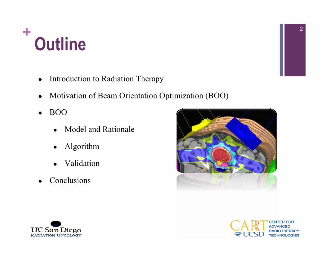
l Introduction to Radiation Therapy
l Motivation of Beam Orientation Optimization (BOO)
l BOO
l Model and Rationale
l Algorithm
l Validation
l Conclusions
+Radiotherapy
3
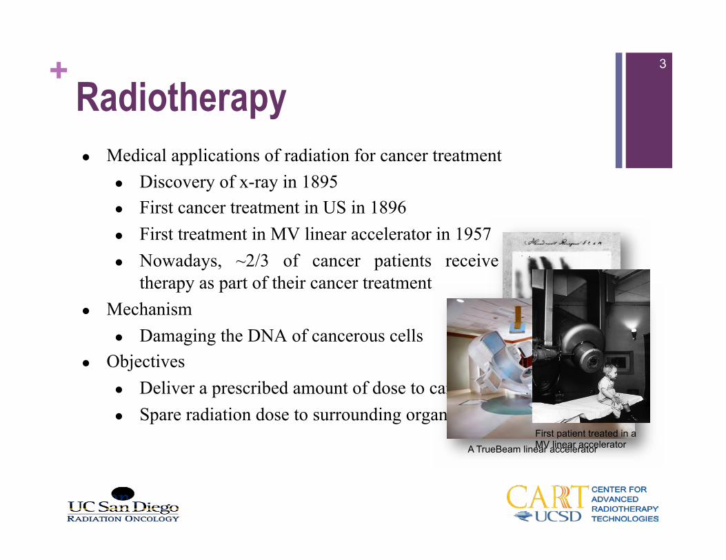
l Medical applications of radiation for cancer treatment l Discovery of x-ray in 1895 l First cancer treatment in US in 1896 l First treatment in MV linear accelerator in 1957 l Nowadays, ~2/3 of cancer patients receive radiation
therapy as part of their cancer treatment l Mechanism
l Damaging the DNA of cancerous cells l Objectives
l Deliver a prescribed amount of dose to cancerous target l Spare radiation dose to surrounding organs First medical X-ray by Wilhelm
Röntgen of his wife's hand
A TrueBeam linear accelerator First patient treated in a MV linear accelerator
+Linear Accelerator
4
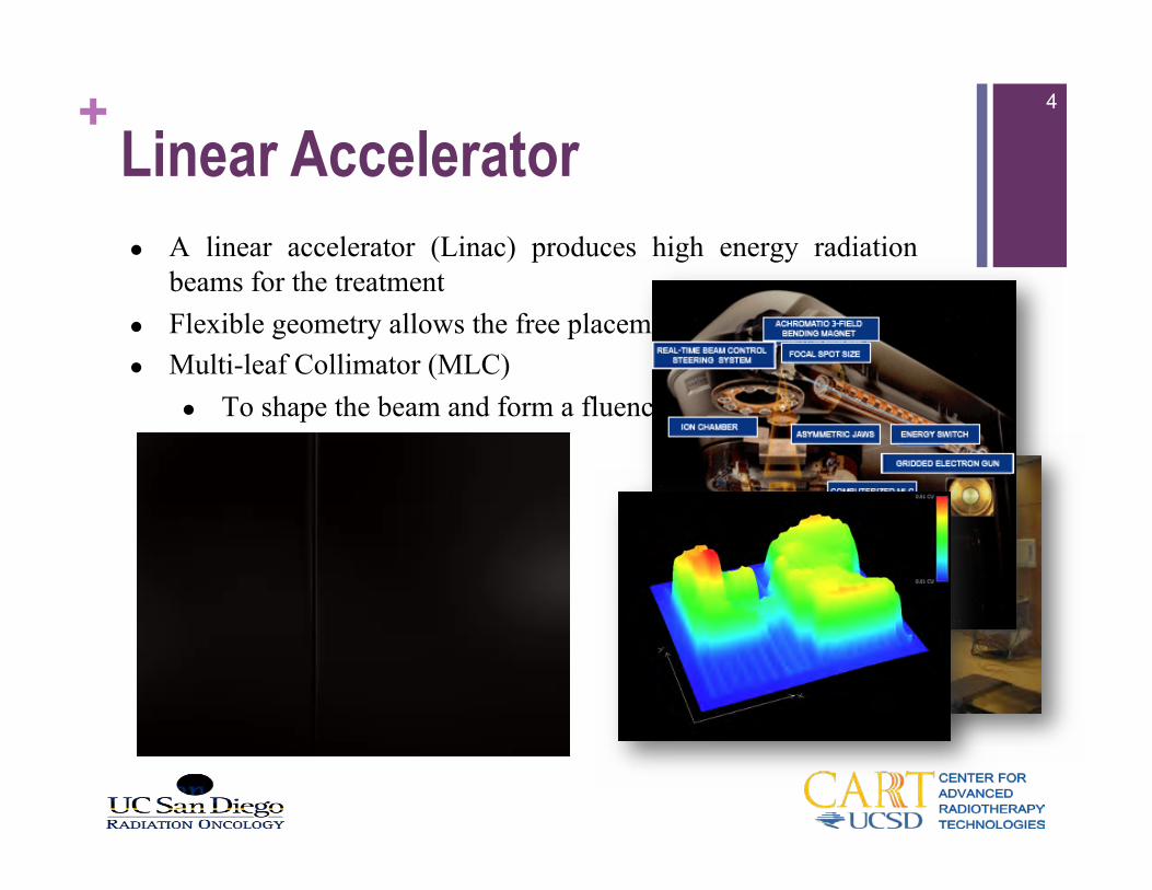
l A linear accelerator (Linac) produces high energy radiation beams for the treatment
l Flexible geometry allows the free placement of beam angles l Multi-leaf Collimator (MLC)
l To shape the beam and form a fluence map
+IMRT
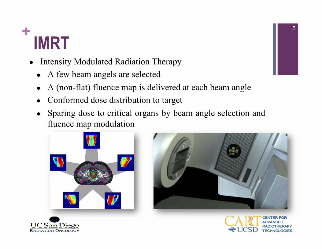
l Intensity Modulated Radiation Therapy l A few beam angels are selected l A (non-flat) fluence map is delivered at each beam angle l Conformed dose distribution to target l Sparing dose to critical organs by beam angle selection and
fluence map modulation
5
+Mathematical View
6
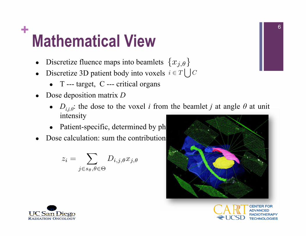
l Discretize fluence maps into beamlets l Discretize 3D patient body into voxels
l T --- target, C --- critical organs l Dose deposition matrix D
l Di,j,θ: the dose to the voxel i from the beamlet j at angle θ at unit intensity
l Patient-specific, determined by physical interactions l Dose calculation: sum the contributions from all beamlets
{xj,✓}
zi =X
j2s✓,✓2⇥
Di,j,✓xj,✓
i 2 T
[C
+
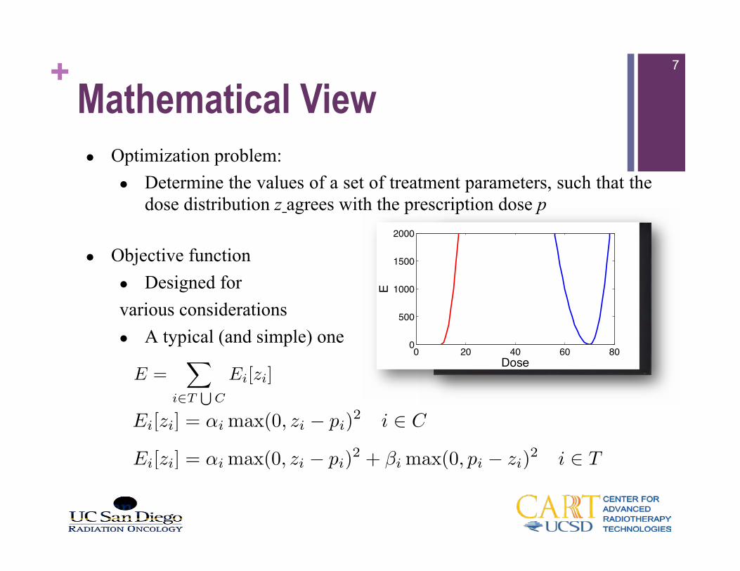
l Optimization problem: l Determine the values of a set of treatment parameters, such that the
dose distribution z agrees with the prescription dose p
l Objective function l Designed for various considerations l A typical (and simple) one
Mathematical View
0 20 40 60 800
500
1000
1500
2000
DoseE
7
Ei[zi] = ↵i max(0, zi − pi)2
i 2 C
Ei[zi] = ↵i max(0, zi − pi)2 + βi max(0, pi − zi)
2i 2 T
E =X
i2TS
C
Ei[zi]
+
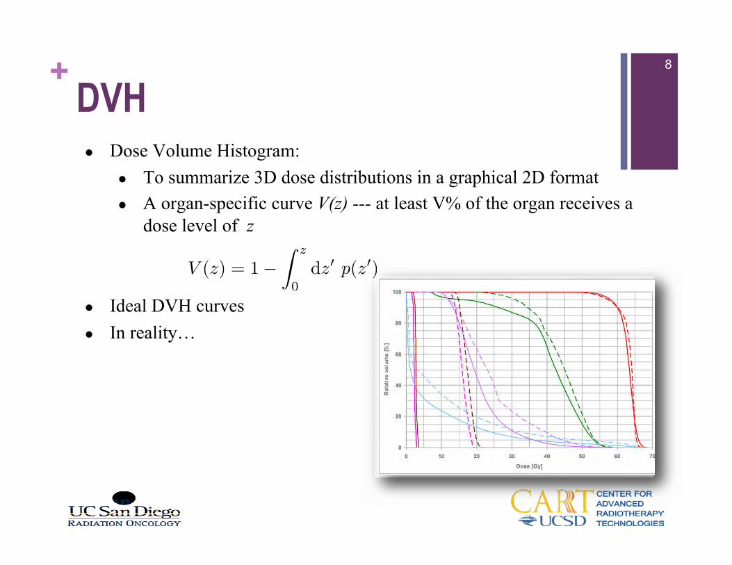
l Dose Volume Histogram: l To summarize 3D dose distributions in a graphical 2D format l A organ-specific curve V(z) --- at least V% of the organ receives a
dose level of z
l Ideal DVH curves l In reality…
DVH 8
V (z) = 1Z z
0
dz0 p(z0)
+Beam Orientation Optimization
9
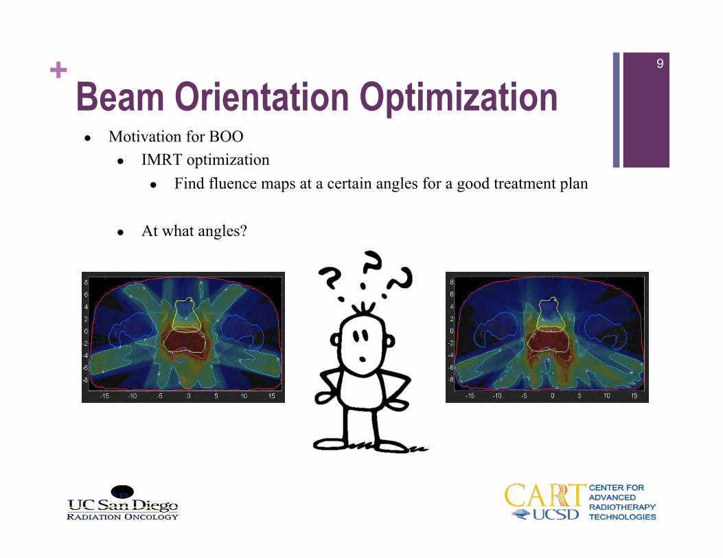
l Motivation for BOO l IMRT optimization
l Find fluence maps at a certain angles for a good treatment plan
l At what angles?
+ 10
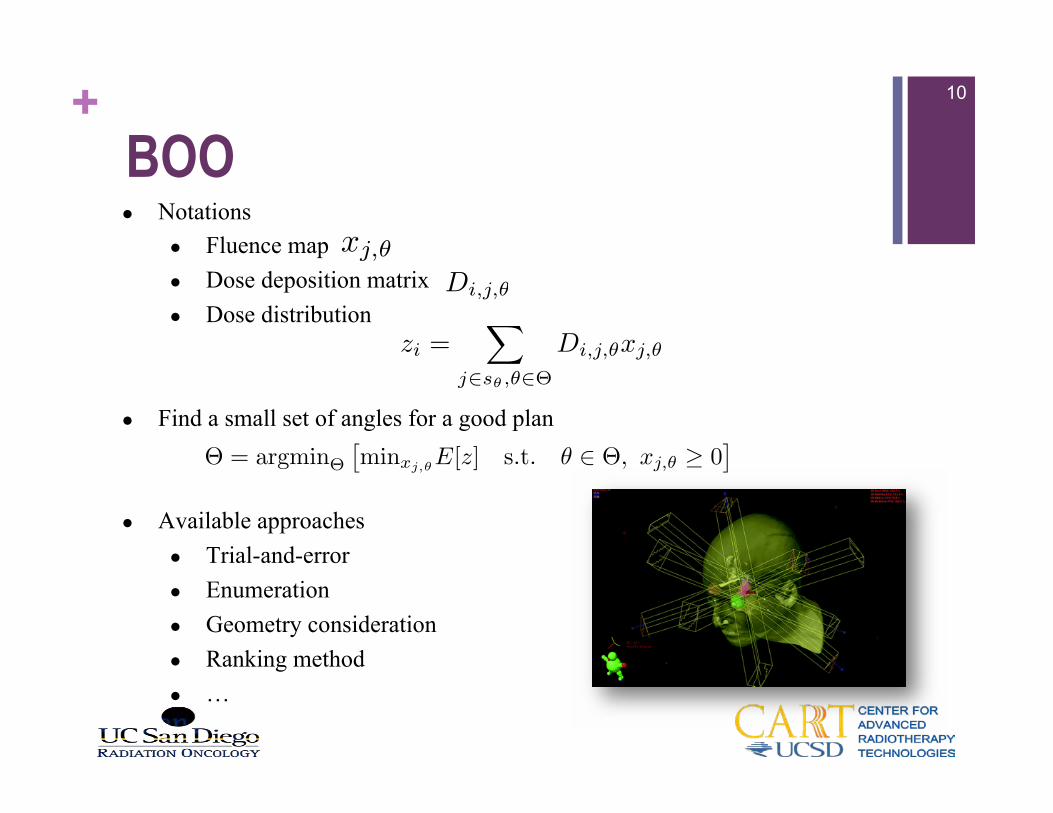
l Notations l Fluence map l Dose deposition matrix l Dose distribution
l Find a small set of angles for a good plan
l Available approaches l Trial-and-error l Enumeration l Geometry consideration l Ranking method l …
BOO
⇥ = argmin⇥⇥minxj,✓
E[z] s.t. ✓ 2 ⇥, xj,✓ ≥ 0⇤
zi =X
j2s✓,✓2⇥
Di,j,✓xj,✓
xj,✓
Di,j,✓
+Model
11
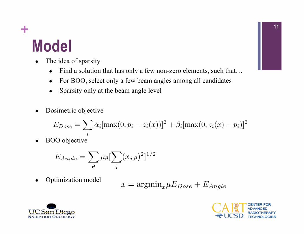
l The idea of sparsity l Find a solution that has only a few non-zero elements, such that… l For BOO, select only a few beam angles among all candidates l Sparsity only at the beam angle level
l Dosimetric objective
l BOO objective
l Optimization model
EDose =X
i
↵i[max(0, pi zi(x))]2 + βi[max(0, zi(x) pi)]
2
EAngle =X
✓
µ✓[X
j
(xj,✓)2]1/2
x = argminxµEDose + EAngle
+L21 Norm
12
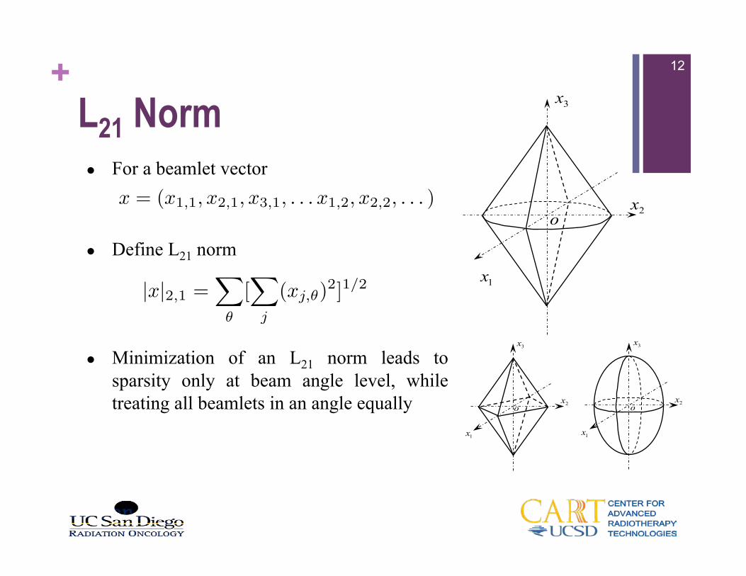
l For a beamlet vector
l Define L21 norm
l Minimization of an L21 norm leads to sparsity only at beam angle level, while treating all beamlets in an angle equally
2x
3x
o
1x
x = (x1,1, x2,1, x3,1, . . . x1,2, x2,2, . . . )
|x|2,1 =X
✓
[X
j
(xj,✓)2]1/2
1x
2x
3x
o
1x
2x
3x
o
+Algorithm
13
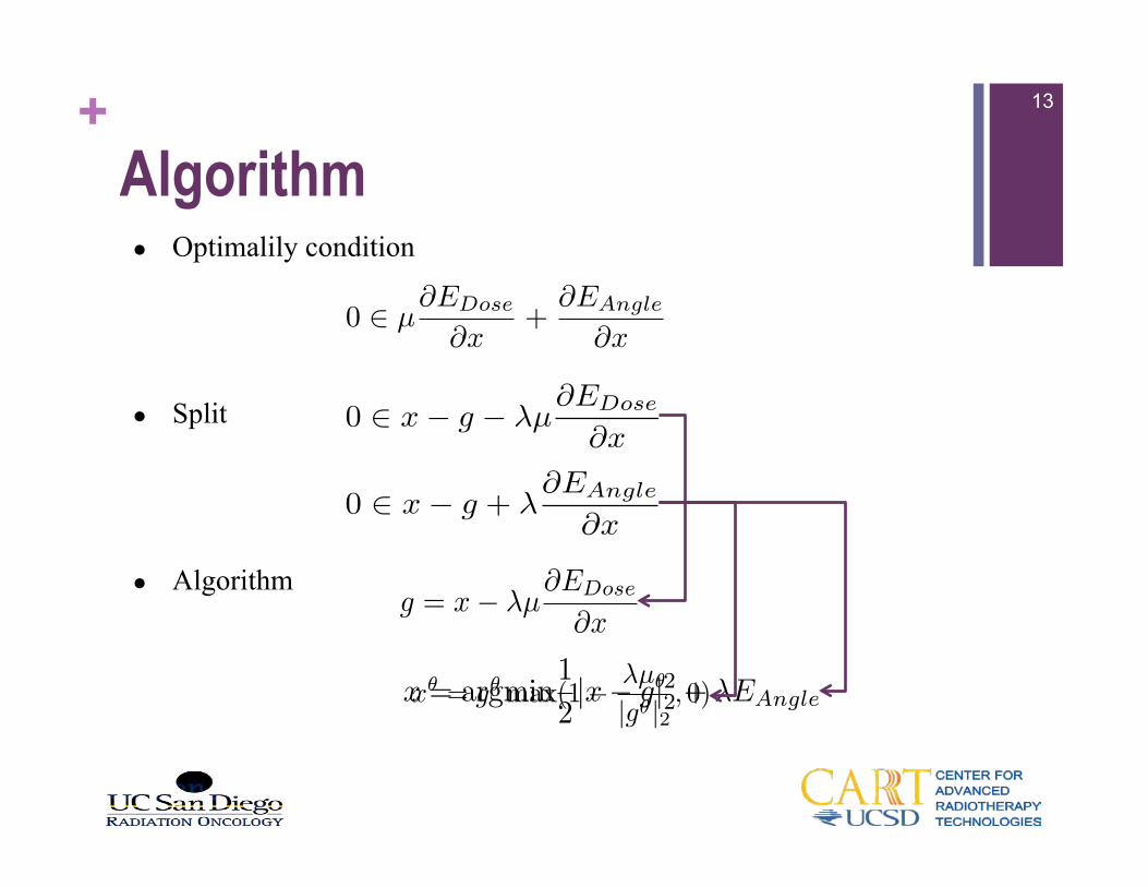
l Optimalily condition
l Split
l Algorithm
0 2 µ
@EDose
@x
+@EAngle
@x
0 2 x− g − λµ
@EDose
@x
0 2 x− g + λ
@EAngle
@x
g = x λµ
@EDose
@x
x = argmin1
2|x g|22 + EAnglex
✓ = g
✓ max(1 µ✓
|g✓|2, 0)
+Algorithm
14
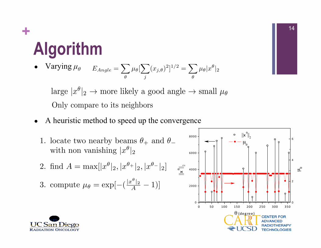
l Varying µθ
l A heuristic method to speed up the convergence
0
2000
4000
6000
8000
||xθ ||2
θ (deg ree)
||x θ||2
0 50 100 150 200 250 300 3500
2
4
6
µ θ
µθ
large |x✓|2 ! more likely a good angle ! small µ✓
Only compare to its neighbors
EAngle =X
✓
µ✓[X
j
(xj,✓)2]1/2 =
X
✓
µ✓|x✓|2
1. locate two nearby beams ✓+ and ✓with non vanishing |x✓|2
2. find A = max[|x✓|2, |x✓+ |2, |x✓ |2]
3. compute µ✓ = exp[( |x✓|2A 1)]
+Algorithm
15
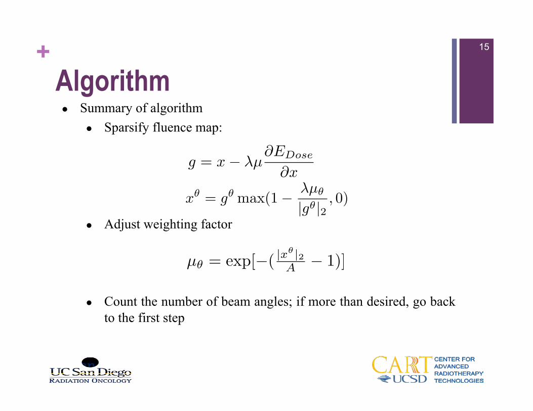
l Summary of algorithm l Sparsify fluence map:
l Adjust weighting factor
l Count the number of beam angles; if more than desired, go back to the first step
g = x λµ
@EDose
@x
x
✓ = g
✓ max(1 µ✓
|g✓|2, 0)
µ✓ = exp[( |x✓|2A 1)]
+Iteration Process
16
0 500 1000 1500
1x10⁴
2x10⁴
850 900 950 1000 1050
4000
4800
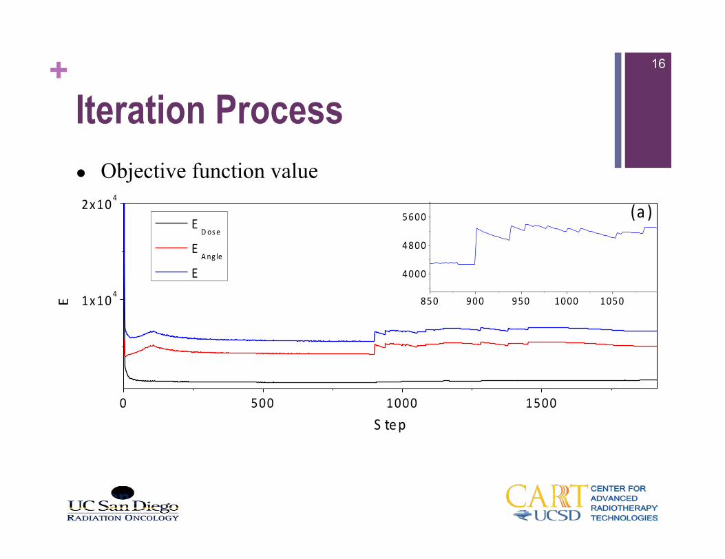
5600 (a )
E
S tep
EDos e
EAng le
E
l Objective function value
+Iteration Process
17
0.0
4.0x10²
8.0x10²
(e)(d)(c )
-
-
-
||xθ ||
2
(b)
0.0
2.0x10³
4.0x10³
--
-
-
0 .0
5.0x10³
1.0x10⁴
---
-
0 .0
5.0x10³
1.0x10⁴
- -
-
0 100 200 300
1.0
2.0
3.0 (f)
-
-
µ θ
θ-(deg ree)
(g )
0 100 200 300
1.0
2.0
3.0-
-
θ-(deg ree)
0 100 200 300
1.0
2.0
3.0
-
-
θ-(deg ree)
0 100 200 300
1.0
2.0
3.0 (i)(h)-
- -
θ-(deg ree)
+Results
18
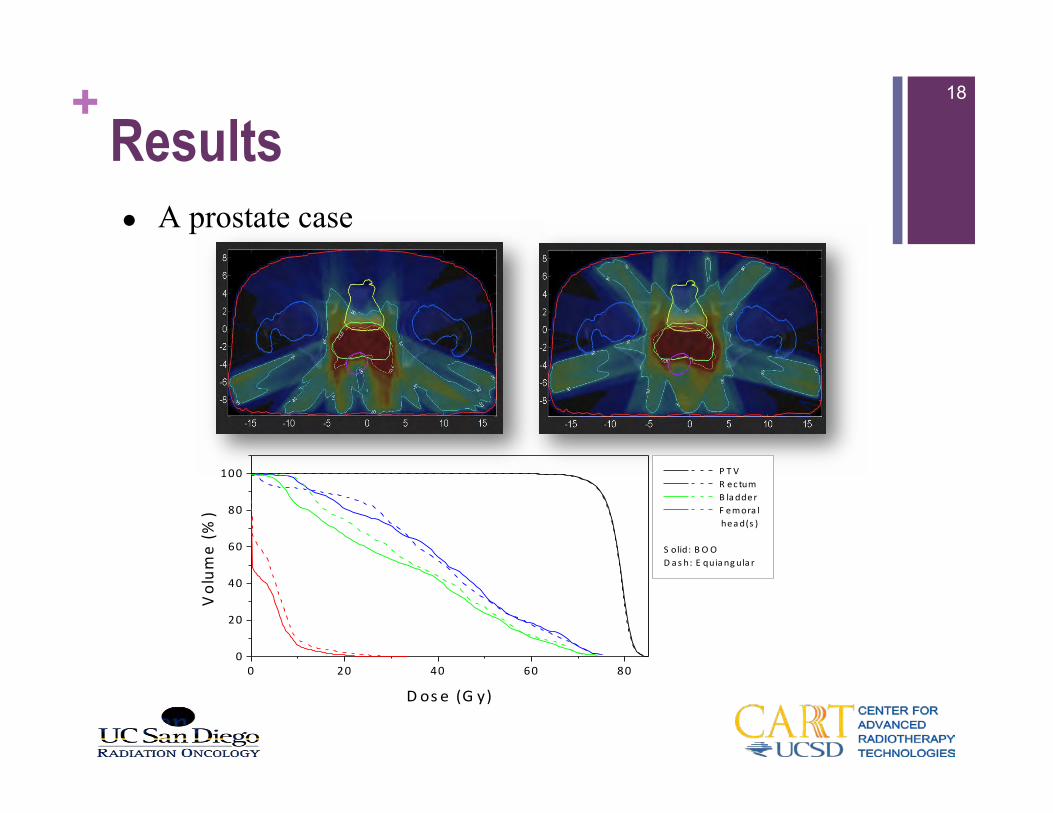
l A prostate case
0 20 40 60 800
20
40
60
80
100 P T V R ec tum B ladder F emora l
head(s )
S olid: B O OD as h: E quiangula r
Vol
ume
(%)
D os e (G y)
+Results
19
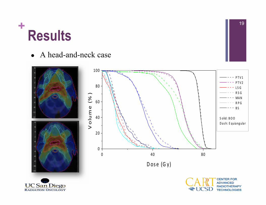
l A head-and-neck case
0 40 800
20
40
60
80
100 P T V 1 P T V 2 L S G R S G MAN R P G B S
S olid: B O OD as h: E quiangula r
Vo
lum
e (
%)
D os e (G y)
+Varying Beam Angles
20
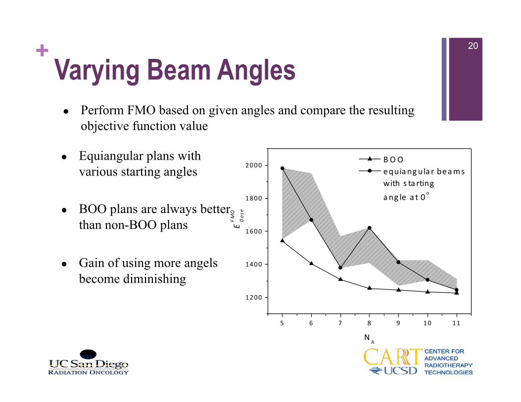
l Equiangular plans with various starting angles
l BOO plans are always better than non-BOO plans
l Gain of using more angels become diminishing
5 6 7 8 9 10 11
1200
1400
1600
1800
2000 B O O equiangula r beams
with s ta rting ang le a t 0 o
EFMO
Dos
e
NA
l Perform FMO based on given angles and compare the resulting objective function value
+Objective Function Values
21
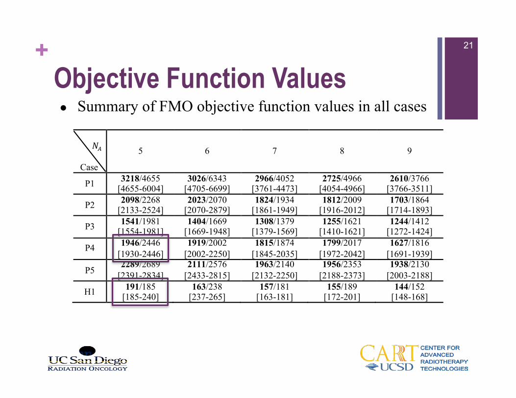
l Summary of FMO objective function values in all cases
!! !!
Case
5 6 7 8 9
P1 3218/4655 [4655-6004]
3026/6343 [4705-6699]
2966/4052 [3761-4473]
2725/4966 [4054-4966]
2610/3766 [3766-3511]
P2 2098/2268 [2133-2524]
2023/2070 [2070-2879]
1824/1934 [1861-1949]
1812/2009 [1916-2012]
1703/1864 [1714-1893]
P3 1541/1981 [1554-1981]
1404/1669 [1669-1948]
1308/1379 [1379-1569]
1255/1621 [1410-1621]
1244/1412 [1272-1424]
P4 1946/2446 [1930-2446]
1919/2002 [2002-2250]
1815/1874 [1845-2035]
1799/2017 [1972-2042]
1627/1816 [1691-1939]
P5 2289/2689
[2391-2834] 2111/2576
[2433-2815] 1963/2140
[2132-2250] 1956/2353
[2188-2373] 1938/2130
[2003-2188]
H1 191/185 [185-240]
163/238 [237-265]
157/181 [163-181]
155/189 [172-201]
144/152 [148-168]
+Discussions
22
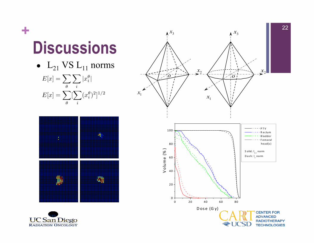
l L21 VS L11 norms
1x
2x
3x
o 2x
3x
o
1x
0 20 40 60 800
20
40
60
80
100 P T V R ec tum B ladder F emora l
head(s )
S olid: l2,1 norm
D as h: l1 norm
Volum
e (%
)
D os e (G y)
E[x] =X
✓
X
i
|x✓i |
E[x] =X
✓
[X
i
(x✓i )
2]1/2
+Conclusion
23
l Beam Orientation Optimization
l It can be approximately solved by an L21 minimization
approach and the problem is convex
l We developed an efficient algorithm to solve the optimization
problem
l We have validated this approach in patient cases
l L21 is a good approximation to the BOO problem
+Acknowledgement
24
l Collaborators on this project l Dr. Steve B. Jiang, UCSD l Dr. Chunhua Men, Elekta l Dr. Yifei Lou, UCLA
l Many other collaborators l The whole CART group