bdd-baseddecisionprocedures forthe modal logic kvardi/papers/jancl06.pdf ·...
TRANSCRIPT
BDD-Based Decision Procedures for the ModalLogic K
1
Guoqiang Pan* — Ulrike Sattler** — Moshe Y. Vardi***
* Department of Computer Science, Rice University, Houston,Texas, 77005, USA.
** School of Computer Science, University of Manchester, Oxford Road, ManchesterM13 9PL, UK
*** Department of Computer Science, Rice University, Houston,Texas, 77005, USA.
ABSTRACT.We describe BDD-based decision procedures for the modal logic K. Our approachis inspired by the automata-theoretic approach, but we avoid explicit automata construction.Instead, we compute certain fixpoints of a set of types—whichcan be viewed as an on-the-flyemptiness of the automaton. We use BDDs to represent and manipulate such type sets, andinvestigate different kinds of representations as well as a“level-based” representation scheme.The latter turns out to speed up construction and reduce memory consumption considerably.We also study the effect of formula simplification on our decision procedures. To prove theviability of our approach, we compare our approach with a representative selection of otherapproaches, including a translation ofK to QBF. Our results indicate that the BDD-basedapproach dominates for modally heavy formulae, while search-based approaches dominate forpropositionally heavy formulae.
KEYWORDS:Modal Logic, Binary Decision Diagram
1. Introduction
In the last 20 years, modal logic has been applied to numerousareas of com-puter science, including artificial intelligence [BRA 94, MCC 69], program verifica-tion [CLA 86, PRA 76, PNU 77], hardware verification [BOC 82, REI 83], databasetheory [CAS 82, LIP 77], and distributed computing [BUR 88, HAL 90]. In theseapplications, deciding satisfiability of a modal formula isone of the most basic rea-
1. Portions of this paper have been presented at CADE-18 and CADE-19.
Journal of Applied Non-Classical Logics.Volume - – No. 2/2006
2 JANCL – -/2006. Special Issue on Implementation of Logics
soning problems, and various techniques have been developed and optimized to de-cide it. Since satisfiability of even the smallest normal modal logic,K, is PSPACE-complete [LAD 77, STO 77, HAL 92], it is clear that different techniques are use-ful for inputs of different characteristics, and that it is unlikely that one techniquewould be able to always outperform others. As modal logic extends propositionallogic, the study in modal satisfiability is deeply connectedwith that of propositionalsatisfiability. For example, tableau-based decision procedures forK are presentedin [LAD 77, HAL 92, PAT 99]. Such methods are built on top of thepropositionaltableau construction procedure by forming a fully expandedpropositional tableauand generating successor nodes “on demand”. A similar method uses the Davis-Logemann-Loveland method [DAV 62] as the propositional engine by treating allmodal subformulae as propositions and, when a satisfying assignment is found, check-ing modal subformulae for the legality of this assignment [GIU 00, TAC 99]. In thelast years, we have seen efforts to combine the optimizations used in tableau andDPLL based approaches. For example, using semantic branching and Boolean con-straint propagation in a tableau-based solver made DLP and FaCT some of the fastestK solvers [PAT 99].
Non-propositional methods take a different approach to theproblem. It has beenshown recently that, by embeddingK into first order logic, a first-order theoremprover can be used for deciding modal satisfiability [HUS 00,ARE 00]. The latterapproach works nicely with a resolution-based first-order theorem prover, which canbe used as a decision procedure for modal satisfiability by using appropriate reso-lution strategies [HUS 00]. Other approaches for modal satisfiability such as mo-saics, type elimination, or automata-theoretic approaches are well-suited for prov-ing exact upper complexity bounds, but are rarely used in actual implementations[BLA 01, HAL 92, VAR 97].
In this paper, we restrict our attention to the smallest normal modal logicK, anddescribe a novel approach to decide the satisfiability of formulae in this logic. Thebasic algorithms presented here are inspired by the automata-theoretic approach forlogics with the tree-model property [VAR 97]. In that approach, one proceeds in twosteps. First, an input formula is translated to a tree automaton that accepts all tree mod-els of the formula. Second, the automaton is tested for non-emptiness, i.e., whetherit accepts some tree. In our approach, we combine, in essence, the two steps, andwe carry out the non-emptiness test without explicitly constructing the automaton.As pointed out in [BAA 01], the inverse method described in [VOR 01] can also beviewed as an application of the automata-theoretic approach that avoids an explicitautomata construction.
The logicK is simple enough that the automaton’s non-emptiness test consistsof a single fixpoint computation, which starts with a set of states and then repeat-edly applies a monotone operator until a fixpoint is reached.1 In the automaton thatcorresponds to a formula, each state is atype, i.e., a set of formulae satisfying someconsistency conditions. The algorithms presented here allstart from some set of types,
1. This approach can be easily extended toK (m).
BDD-based Decision Procedures forK 3
and then repeatedly apply a monotone operator until a fixpoint is reached: either theystart with the set ofall types and remove those types with “possibilities”3ϕ for whichno “witness” can be found, or they start with the set of types having no possibilities3ϕ, and add those types whose possibilities are witnessed by a type in the set. Thetwo approaches, top-down and bottom-up, corresponds to thetwo ways in which non-emptiness can be tested for automata forK : via a greatest fixpoint computation forautomata on infinite trees or via a least fixpoint computationfor automata on finitetrees. The bottom-up approach is closely related to the inverse method described in[VOR 01], while the top-down approach is reminiscent of the type-elimination methoddeveloped for propositional dynamic logic in [PRA 80].
The key idea underlying our implementation is that of representing sets of typesand operating on them symbolically. Our implementation uses Binary Decision Di-agrams (BDDs) [BRY 86]: BDDs are compact representations ofpropositional for-mulae, and are commonly used as a compact representation of states. One of theiradvantages is that they come with efficient operations for certain manipulations. Byrepresenting a set of types by a BDD, we are able to symbolically construct fixpointtype sets efficiently.
We then study optimization issues for BDD-basedK solvers. First, we focus onalternative representations that can be used for a set of states. Types exert a strictconsistency requirement on the assignment to related subformulae, which is a majorfactor in the size of the BDD used to represent the type sets. For example, if a typecontains a conjunction, then it must also contain both conjuncts. For the type-basedapproach, we have employed thebox normal form: negation can only be applied toatoms or box formulae (and no diamonds are available). In contrast, in what we calltheparticle-based approach, we employ the standard negation normal form, and thusdeal with both diamond and box formulae.
Secondly, for both the type- and the particle-approach, we investigate aleanap-proach: intuitively, our lean sets only capture the minimal, atomic information. E.g.,conjunctions are only implicitly represented by the presence of both conjuncts. Thisclearly reduces BDD size, but also makes the manipulation ofBDDs more complex.
Thirdly, we take advantage of the properties ofK, namely the finite-tree-modelproperty. A set of types/particles can be seen to encode a model for the formula. Byconsidering a layered model instead of a general model, we modify the bottom-upprocedure so that each step only checks witness for diamond operators occurring at aspecific depth. This approach yields further performance improvements.
Fourthly, we turn to a pre-processing optimization. The idea is to apply some light-weight reasoning to simplify the input formula before starting to apply heavy-weightBDD operations. In the propositional case, a well-known preprocessing rule is thepure-literal rule [DAV 62]. Preprocessing has also been shown to be usefulfor linear-time formulae [SOM 00, ETE 00]. Our preprocessing is based ona modal pure-literalsimplification which takes advantage of the tree-model property ofK. We show thatadding preprocessing yields fairly significant performance improvements, enabling usto handle the hard formulae of TANCS 2000[MAS 00].
4 JANCL – -/2006. Special Issue on Implementation of Logics
Finally, we also focus on BDD-specific optimizations on our implementation of thealgorithm. Besides using optimized image finding techniques like conjunctive clus-tering with early quantification [BUR 91, GEI 94, RAN 95, CIM 00], we also studythe issue of variable order, which is known to be of critical importance to BDD-based algorithms. The performance of BDD-based crucially depends on the size ofthe BDDs and variable order is a major factor in determining BDD size, as a “bad”order may cause an exponential blow-up [BRY 86]. While finding an optimal variableorder is known to be intractable [TAN 93], heuristics often work quite well in prac-tice [RUD 93]. We focus here on finding a good initial variableorder tailored to theapplication at hand, but for large problem instances we haveno choice but to invokedynamic variable ordering, provided by the BDD package. Ourfinding is that choos-ing a good initial variable order does improve performance,but the improvement israther modest.
This paper describes a viability study for our approach. To compare the differ-ent optimizations of BDD-based approaches, we use existingbenchmarks of modalformulae, TANCS 98 [HEU 96] and TANCS 2000 [MAS 00], and we used *SAT[TAC 99] as a reference. A straightforward implementation of our approach did notyield a competitive implementation, but an optimized implementation did yield a com-petitive implementation, calledKBDD, indicating the viability of our approach.
To assess the competitiveness of our optimized solver, we compare it with thenative solvers *SAT and DLP as well as the translation-basedsolver MSPASS. Ad-ditionally, we also developed a translation fromK to QBF (which is of independentinterest), and applied semprop, which is a highly optimizedQBF solver [LET 02]. Ourresults indicate that the BDD-based approach dominates formodally heavy formulaewhile search-based approaches dominate for propositionally-heavy formulae.
The paper is organized as follows. After introducing the modal logic K in Sec-tion 2, we present our algorithms and show them to be sound andcomplete in Sec-tion 3. In Section 4, we discuss four optimizations that we applied. In Section 5, wepresent a BDD-based implementation. An embedding ofK into QBF is presented inSection 6. Finally, we present the empirical evaluation, both between different opti-mizations in the BDD-based framework and with other solvers, in Section 7.
2. Preliminaries
In this section, we introduce the syntax and semantics of themodal logicK, aswell as types and how they can be used to encode a Kripke structure.
The set ofK formulae is constructed from a set of propositional variablesΦ ={q1, q2, . . .}, and is the least set containingΦ that is closed under the Boolean oper-ators∧ and¬ and the unary modality2. As usual, we introduce the other Booleanoperators as abbreviations, and3ϕ as an abbreviation for¬2¬ϕ. The set of proposi-tional variables used in a formulaϕ is denotedAP (ϕ).
BDD-based Decision Procedures forK 5
A formula in K is interpreted in a Kripke structureK = 〈V,W,R,L〉, whereV is a set (containingΦ) of propositional variables,W is a set of possible worlds,R ⊆ W ×W is the accessibility relation on worlds, andL : V → 2W is a labelingfunction for each state, where for a propositionv, L(v) is the set of states wherevholds. The notion of a formulaϕ beingsatisfiedin a worldw of a Kripke structureK(written asK,w |= ϕ) is inductively defined as follows:
–K,w |= q for q ∈ Φ iff w ∈ L(q)
–K,w |= ϕ ∧ ψ iff K,w |= ϕ andK,w |= ψ
–K,w |= ¬ϕ iff K,w 6|= ϕ
–K,w |= 2ϕ iff, for all w′, if (w,w′) ∈ R, thenK,w′ |= ϕ
The abbreviated operators can be interpreted as follows:
–K,w |= ϕ ∨ ψ iff K,w |= ϕ orK,w |= ψ
–K,w |= 3ϕ iff there existsw′ with (w,w′) ∈ R andK,w′ |= ϕ.
A formulaψ is satisfiableif there existK,w with K,w |= ψ. In this case,K is calleda modelof ψ. Two formulaeϕ andψ are said to be equivalent if, for all structuresKand all worldsw ∈W ,K,w |= ϕ if and only ifK,w |= ψ.
For our concern here, the most important property ofK is the tree-model prop-erty, which allows automata-theoretic approaches to be applied. In fact, it has thestrongerfinite-tree-model property, which will allow both top-down and bottom-upconstruction of such automata.
THEOREM 1 ([BLA 01]). — K has the finite-tree-model property, i.e., every sat-isfiable formulaϕ has a modelK,w such thatR is a finite tree with rootw0 andK,w0 |= ϕ.
In fact, a formulaψ has a finite tree model that is only as deep as itsmodal depth,which we define next as usual; and we will use this “small tree model” property forthe “level” optimizations in our algorithm.
Given a formulaψ, call its set of subformulaesub(ψ). Forϕ ∈ sub(ψ), we definedepth(ϕ) as follows:
– if ϕ ∈ Φ, thendepth(ϕ) = 0;
– if ϕ = ¬ϕ′, thendepth(ϕ) = depth(ϕ′);
– If ϕ = ϕ′ ∧ϕ′′ orϕ = ϕ′ ∨ϕ′′, thendepth(ϕ) = max{depth(ϕ′), depth(ϕ′′)},
– If ϕ = 2ϕ′ orϕ = 3ϕ′, thendepth(ϕ) = depth(ϕ′) + 1.
We restrict our attention to formulae in a certain normal form. A formulaψ is saidto be inbox normal form(BNF) if all its subformulae are of the formϕ ∧ ϕ′, ϕ ∨ ϕ′,2ϕ, ¬2ϕ, q, or¬q whereq ∈ AP (ψ). EachK formulae can be obviously convertedinto an equivalent one in BNF that is of linear size. If not stated otherwise, we assumeall formulae to be in BNF.

6 JANCL – -/2006. Special Issue on Implementation of Logics
The closureof a formulacl(ψ) is defined as the smallest set such that, for allsubformulaeϕ of ψ, if ϕ is not of the form¬ϕ′, then{ϕ,¬ϕ} ⊆ cl(ψ). Please notethatcl(ψ) may contain negated conjunctions and negations, and thus formulae that arenot in BNF. We write∼ ϕ to represent¬ϕ if ϕ is positive andϕ′ if ϕ = ¬ϕ′.
The first algorithms we present work ontypes, i.e., maximal sets of formulae thatare consistent w.r.t. the Boolean operators, and where (negated) box formulae aretreated as atoms. A set of formulaea ⊆ cl(ψ) is called aψ-type(or simply a typeif ψ is clear from the context) if it satisfies the following conditions:
– If ϕ = ¬ϕ′, thenϕ ∈ a iff ϕ′ /∈ a.
– If ϕ = ϕ′ ∧ ϕ′′, thenϕ ∈ a iff ϕ′ ∈ a andϕ′′ ∈ a.
– If ϕ = ϕ′ ∨ ϕ′′, thenϕ ∈ a iff ϕ′ ∈ a orϕ′′ ∈ a.
For a set of typesA, we define a maximal accessibility relation∆ ⊆ A×A as follows.
∆(a, a′) iff for all 2ϕ′ ∈ a, we haveϕ′ ∈ a′.
Given a set of typesA ⊆ 2cl(ψ), we can construct a Kripke structureKA using∆ asfollows: KA = 〈AP (ψ), A,∆, L〉 with a ∈ L(q) iff q ∈ a. Such a Kripke structureKA is almosta canonical model [BLA 01]—the only difference can be seen whentrying to prove thatKA satisfies, for allϕ ∈ cl(ψ):
CLAIM 2. — KA, a |= ϕ iff ϕ ∈ a.
This statement is clearly true for atomic and propositionalϕ by definition of types,and it is also true forϕ = 2ϕ′ by construction of∆. The only case that fails is thecaseϕ = ¬2ϕ′ ∈ a: it might be the case thatϕ′ ∈ b for all b with ∆(a, b). If thisis the case, then we say that the negated box formula¬2ϕ′ in a is not witnessedbyany b in A. In the following section, we will describe operators on type sets whosefixpointA then indeed satisfies Claim 2.
3. Our algorithms
The two algorithms presented here take a certain initial setof types and repeatedlyapply a monotone operator to it. If this application reachesa fixpointA, we canshow that the above construction ofKA indeed satisfies Claim 2, i.e., all negated boxformulae are indeed “witnessed” by someb ∈ A. This Kripke structure is then amodel ofψ iff ψ ∈ a for somea ∈ A.
The first algorithm follows a “top-down” approach, i.e., it starts with the setA ⊆2cl(ψ) of all propositionally consistent types, and the monotone operator removes thosetypes containing negated box formulae which are not witnessed in the current set oftypes. Dually, the second, “bottom-up” approach starts with the set of types that do notcontain negated box formulae, and then adds those types whose negated box formulaeare witnessed in the current set of types.
BDD-based Decision Procedures forK 7
In the following, we will call our class of algorithmsKBDD since we intend touse BDD as the type set representation.
Both algorithms follow the following scheme:
X ⇐ Init(ψ)repeatX ′ ⇐ XX ⇐ Update(X ′)
until X = X ′
if existsx ∈ X such thatψ ∈ x thenreturn “ψ is satisfiable”
elsereturn “ψ is not satisfiable”
end if
Since this algorithm is operating with elements in a finite lattice 2cl(ψ) and usesa monotoneUpdate(·) operator, it obviously terminates. In fact, after defining thesetwo operators, we will show that it will terminate indepth(ψ) + 1 iterations.
3.1. Top-down approach
The top-down approach is closely related to the type elimination approach whichis, in general, used for more complex modal logics, see, e.g., Section 6 of [HAL 92].For the top-down algorithm, the functionsInit(ψ) andUpdate(·) are defined as fol-lows:
– Init(ψ) is the set ofall ψ-types.
– Update(A) := A \ bad(A), wherebad(A) are the types inA that contain un-witnessed negated box formulae. More precisely,
bad(A) := {a ∈ A | there exists¬2ϕ ∈ a and, for allb ∈ A with ∆(a, b),we haveϕ ∈ b}.
THEOREM 3. — The top-down algorithm decides satisfiability ofK formulae.
PROOF. — LetA be the set of types that is the fixpoint of the top-down algorithm,i.e., Update(A) = A. We useA0 for Init(ψ) andAi for the set of types afteriiterations. SinceUpdate(·) is monotone and eachAi is a subset of the finitecl(ψ),the top-down algorithm terminates. More precisely, all thetypes inAi that containunwitnessed negated box formulasϕ with depth(ϕ) > i are removed inAi+1. As aconsequence, the algorithm stops after at mostdepth(ψ) + 1 iterations. To finish theproof, it thus suffices to prove soundness and completeness.
CLAIM 4 (SOUNDNESS). — For each typea ∈ A and formulaϕ ∈ cl(ψ), if ϕ ∈ a,thenKA, a |= ϕ.
By induction on the structure of formulae:
8 JANCL – -/2006. Special Issue on Implementation of Logics
– if ϕ = q or ϕ = ¬q for q ∈ AP (ψ), thenKA, a |= ϕ iff ϕ ∈ a by constructionof L.
– For the inductive case, assume the claim holds on all formulas incl(ϕ) − {ϕ,∼ϕ}.
– if ϕ = ϕ′∧ϕ′′, orϕ = ϕ′∨ϕ′′, the claim follows immediately by induction andthe definition of types.
– if ϕ = ¬(ϕ′ ∧ ϕ′′), thenϕ ∈ a implies thatϕ′ 6∈ a or ϕ′′ 6∈ a since, otherwise,ϕ′ ∧ ϕ′′ would be ina. By maximality ofa, this implies that∼ ϕ′ ∈ a or ∼ ϕ′′ ∈ a,and thus we haveKA, a |= ¬ϕ′ orKA, a |= ¬ϕ′′ by induction. HenceKA, a |= ¬ϕ.
– the caseϕ = ¬(ϕ′ ∨ ϕ′′) is completely analogous.
– let ϕ = 2ϕ′ ∈ a. The definition of∆ implies thatϕ′ ∈ a′ for all a′ with∆(a, a′). By induction,KA, a
′ |= ϕ′, for all a′ with ϕ′ ∈ a′, and thusKA, a |= 2ϕ′ .
– if ϕ = ¬2ϕ′ ∈ a, thena /∈ bad(A) becauseUpdate(A) = A, and thus thereexistsb ∈ A with ∆(a, b) andϕ′ /∈ b. By definition of types,∼ ϕ′ ∈ b, and thus wehaveKA, b |= ¬ϕ′ by induction. HenceKA, a |= ¬2ϕ′.
CLAIM 5 (COMPLETENESS). — For all ϕ in cl(ψ), if ϕ is satisfiable, then thereexists somea ∈ A with ϕ ∈ a.
Given a satisfiable formulaϕ, take a modelK = 〈AP (ψ),W,R,L〉withK,wϕ |=ϕ. For a worldw ∈ W , we define its typea(w) = {̺ ∈ cl(ψ) | K,w |= ̺}, andwe defineA(W ) = {a(w) | w ∈ W}. Obviously, due to the semantics of the boxmodality and the definition ofa(·), R(v, w) implies∆(a(v), a(w)). Then we show,by induction oni, thatA(W ) ⊆ Ai. Sinceϕ ∈ a(wϕ) by construction, this proves theclaim.
– A(W ) ⊆ A0 sinceA0 containsall typesa ⊆ cl(ψ).
– LetA(W ) ⊆ Ai and assume thatA(W ) * Ai+1. Then there is somew ∈ Wsuch thata(w) ∈ bad(Ai). So there is some¬2̺ ∈ a(w) and, for allb ∈ Ai with∆(a(w), b), we have̺ ∈ b. Hence there is nov ∈ W with R(w, v) andK, v |= ¬̺,in contradiction toK,w |= ¬2̺.
■
3.2. Bottom-up approach
As mentioned above, the top-down algorithm starts with all valid types, and repeat-edly removes types with unwitnessed formulae. In contrast,the bottom-up algorithmstarts with a small set of types (i.e., those without negatedbox formulae), and re-peatedly adds those types whose negated box formulae are witnessed in the currentset. For the bottom-up approach, the functionsInit(ψ) andUpdate(·) are defined asfollows:
BDD-based Decision Procedures forK 9
– Init(ψ) is the set of all those types that do not require any witnesses, whichmeans that they do not contain any negated box formula or, equivalently, that theycontain all positive box formulae incl(ψ). More precisely,
Init(ψ) := {a ⊆ cl(ψ) | a is a type and2ϕ ∈ a for each2ϕ ∈ cl(ψ)}.
– Update(A) := A ∪ supp(A), wheresupp(A) is the set of those types whosenegated box formulae are witnessed by types inA. More precisely,
supp(A) := {a ⊆ cl(ψ) | a is a type and, for all¬2ϕ ∈ a, there existsb ∈ Awith ∼ ϕ ∈ b and∆(a, b)}.
We say that a type insupp(A) is witnessedby a type inA.
THEOREM 6. — The bottom-up algorithm decides satisfiability ofK formulae.
PROOF. — As in the proof of Theorem 3, we useA for the fixpoint of the bottom-up algorithm,A0 for Init(ψ), andAi for the set of types afteri iterations. Again,Update(·) is monotone andA0 is finite, and thus the bottom-up algorithm terminates.More precisely,Ai+1 is obtained fromAi by adding types containing a formulaϕwith depth(ϕ) > i. As a consequence, the algorithm stops after at mostdepth(ψ)+1iterations. To finish the proof, we prove soundness and completeness.
CLAIM 7 (SOUNDNESS). — For each typea ∈ A and formulaϕ ∈ cl(ψ), if ϕ ∈ a,thenKA, a |= ϕ.
Again, soundness can be proved by induction on the structureof formulae. Werestrict our attention to the only interesting case, namelyϕ = ¬2ϕ′ ∈ a. Letϕ ∈ a.By construction ofA, there is someb ∈ A with ∼ ϕ′ ∈ b and∆(a, b). Thus, byinduction,KA, b |= ¬ϕ′, and thusKA, a |= ϕ. .
CLAIM 8 (COMPLETENESS). — For all ϕ ∈ cl(ψ), if ϕ is satisfiable, then thereexists somea ∈ A with ϕ ∈ a.
It is well-known thatK has the finite-tree-model property (see, e.g. [HAL 92]),i.e., each satisfiableK formulaψ has a model whose relational structure forms a finitetree. Take such a modelK = 〈AP (ψ),W,R,L〉 with K,wϕ |= ϕ, and define themappingsa(·) andA(·) from worlds inK to types as in the proof of Claim 5. Weshow by induction oni that, if i is the maximal distance between a nodew ∈ W andthe leaves ofK ’s subtree rooted atw, thena(w) ∈ Ai. SinceAj ⊆ Aj+1 for all j andK forms a finite tree model ofϕ, this proves the claim.
– If i = 0, thenw is a leaf inK (i.e., there is now′ ∈ W with R(w,w′)), and thusK,w 6|= ¬2ϕ′ holds for all¬2ϕ′ ∈ cl(ψ). Hencea(w) ∈ A0.
– Let i > 0 andw a node withi the maximal distance betweenw and the leaves ofK ’s subtree rooted atw. Then, by induction, for each childw′ of w, we havea(w′) ∈Ai−1. NowR(w,w′) implies∆(a(v), a(w)). Thus, for each¬2ϕ′ ∈ a(w), there issomew′ ∈ W with a(w′) ∈ Ai−1 and¬ϕ′ ∈ a(w′). Thusa(w) ∈ supp(Ai−1) ⊆ Ai.
■
10 JANCL – -/2006. Special Issue on Implementation of Logics
4. Optimizations
The decision procedures described above handle a formula inthree steps. First, theformula is converted into box normal form. Then, the initialset of types is generated—we can think of this set as being represented by a set of bit vectors. Finally, this setis updated through a fixpoint process. The answer of the decision procedure dependson a simple syntactic check of this fixpoint. In this section,we will describe fourorthogonal optimization techniques, working on differentstages in the procedure.
4.1. Particles
The approaches presented so far strongly depend on the fact that we use the boxnormal form, and they can be said to be redundant: if a type contains two conjuncts ofsome subformula of the input, then it also contains the corresponding conjunction—although the truth value of the latter is determined by the truth values of the former.Now we propose a representation where we do not insist on sucha redundancy, whichpossibly reduces the size of the representation of the corresponding sets. To do so, itis convenient to work on formulae in a different normal form.
A K formulaψ is said to be innegation normal form(NNF) if all its subformulaeare of the formϕ∧ϕ′, ϕ∨ϕ′, 2ϕ, 3ϕ, q, or¬q whereq ∈ AP (ψ). It is well-knownthat everyK formula can be converted into an equivalent on in NNF that is of linearsize. When talking about “particles”, we assume that all formulae are in NNF. Asbefore, we usesub(ψ) to denote the set of subformulae ofψ.
A setp ⊆ sub(ψ) is aψ-particle if it satisfies the following conditions:
– If ϕ = ¬ϕ′, thenϕ ∈ p impliesϕ′ /∈ p.
– If ϕ = ϕ′ ∧ ϕ′′, thenϕ ∈ p impliesϕ′ ∈ p andϕ′′ ∈ p.
– If ϕ = ϕ′ ∨ ϕ′′, thenϕ ∈ p impliesϕ′ ∈ p orϕ′′ ∈ p.
Thus, in contrast to a type, a particle may contain bothϕ′ andϕ′′, but neitherϕ′ ∧ ϕ′′
norϕ′ ∨ ϕ′′.
For particles,∆(·, ·) is defined as for types. From a set of particlesP and thecorresponding∆(·, ·), we can construct a Kripke structureKP in the same way asfrom a set of types.
For the top-down approach, the auxiliary functionsInit(·) andUpdate(·) forparticles are defined as follows:
– Init(ψ) is the set of allψ-particles.
– Update(P ) = P \ bad(P ), wherebad(P ) is the particles inP that containunwitnessed diamond formulae, i.e.
bad(P ) := {p ∈ P | there exists3ϕ ∈ p such that, for allq ∈ Pwith ∆(p, q), we haveϕ /∈ q}.
BDD-based Decision Procedures forK 11
THEOREM 9. — The top-down algorithm for particles decides satisfiability of Kformulae.
PROOF. — Termination and the linear bound on the number of iterations are identicalto the one of Theorem 3.
CLAIM 10. — (Soundness) For each particlep ∈ P and formulaϕ ∈ sub(ψ), ifϕ ∈ p, thenKP , p |= ϕ.
The proof is analogous to one of Claim 4, except for the fact that the¬2ϕ′ caseneeds to be replaced with the3ϕ′ one.
– if ϕ = 3ϕ′ ∈ p, thenp /∈ bad(P ) implies that there existsq ∈ P with ∆(p, q)andϕ′ ∈ q. By induction,KP , q |= ϕ′, and thusKP , p |= 3ϕ′.
CLAIM 11. — (Completeness) For all ϕ ∈ sub(ψ), if ϕ is satisfiable, then thereexists somep ∈ P with ϕ ∈ p.
The proof is analogous to the one of Claim 5: we take a modelK of ϕ, generatea particle setP (W ) from the states ofK, and show thatP (W ) ⊆ P by induction onthe number of iterationsi:
– P (W ) ⊂ P 0 sinceP 0 containsall particlesp ⊆ sub(ψ).
– LetP (W ) ⊆ P i and assume thatP (W ) * P i+1. Then there is somew ∈ Ksuch thatp(w) ∈ bad(P i). So there is some3ϕ ∈ p(w) and, for allq ∈ Ai with∆(p(w), q), we haveϕ /∈ q. Hence there is nov ∈ W with R(w, v) andK, v |= ¬ϕ,in contradiction toK,w |= 3ϕ.
■
As for types, we also define a bottom-up algorithm for particles, and we do this bysimply setting our two auxiliary functions accordingly:
– Init(ψ) := {p ⊆ sub(ψ) | p is a particle and3ϕ /∈ p for all 3ϕ ∈ sub(ψ)} isthe set ofψ-particlesp that do not contain diamond formulae.
– Update(P ) := P ∪ supp(P ), wheresupp(P ) is the set of witnessed particlesdefined as follows:
supp(P ) := {p ⊆ sub(ψ) | p is aψ-particle and, for all3ϕ ∈ p,there existsq ∈ P with ϕ ∈ q and∆(p, q)}.
Again, we obtain a decision procedure, and this can be provedas before.
THEOREM 12. — The bottom-up algorithm for particles decides satisfiability of Kformulae.
Just like a set of types can be encoded as a set of bit vectors bya BDD, we canrepresent a set of particles in the same way. It is easy to see that bit vectors for particlesmay be longer than bit vectors for types because, for example, our input may involvesubformulae2p and 3¬p. This, in turn, means that encoding particle sets using
12 JANCL – -/2006. Special Issue on Implementation of Logics
BDDs may require more BDD variables than their encoding of types. The size of theBDD may, however, be smaller for particles since particles impose fewer constraintsthan types.2 Beside a possible reduction in the size required to encode a bit-vectorrepresentation of particle sets, the particle-based approaches also can improve runtime of our algorithms. From the definition ofbad andsupp, we can see that, in thetype-based approaches, for each fixpoint iteration and eachtype, we have to check allbox formulae—even though the “real” test is only required onthe negated ones thatare present in the type considered. In contrast, in the particle-based approaches, weonly have to check all diamond formulae that are subformulaeof the input.
4.2. Lean approaches
Even though the particle approach imposes less constraintsthan the type approach,it still involves redundant information: like types, particles may contain both a con-junction and the corresponding conjuncts. Next, to furtherreduce the size of the cor-responding BDDs, we propose a representation where we only keep track of the “non-redundant” subformulae. We call this variation the lean approach, and we present itfor both the type and the particle approach and, for both top-down and bottom-up.
First, we define a set of “non-redundant” subformulaeatom(ψ) as the set ofthose formulae incl(ψ) that are neither conjunctions nor disjunctions, i.e., eachϕ ∈ atom(ψ) is of the form2ϕ′, q, ¬2ϕ′, or ¬q. By definition of types, eachψ-typea ⊆ cl(ψ), corresponds one-to-one to alean typelean(a) := a ∩ atom(ψ).To specify our algorithms for lean types, we inductively define a relation∈̇ between(non-atomic) formulae and lean types as follows:ϕ ∈̇ a if
– ϕ ∈ atom(ψ) andϕ ∈ a,
– ϕ = ¬ϕ′ and notϕ′ ∈̇ a,
– ϕ = ϕ′ ∧ ϕ′′, ϕ′ ∈̇ a, andϕ′′ ∈̇ a, or
– ϕ = ϕ′ ∨ ϕ′′ andϕ′ ∈̇ a orϕ′′ ∈̇ a.
The top-down and bottom-up approach for types can be easily modified to work forlean types: it suffices to modify the definition of the functionsbad andsupp as follows:
bad(A) := {a ∈ A | there exists¬2ϕ ∈ a and, for allb ∈ A with ∆(a, b),we haveϕ ∈̇ b}.
supp(A) := {a ⊆ cl(ψ) | a is a type and, for all¬2ϕ ∈ a, there existsb ∈ Awith ¬ϕ ∈̇ b and∆(a, b)}.
The following theorem is then a direct consequence of the correctness of our algo-rithms for types: given the one-to-one relationship between types and lean types, we
2. Of course, BDD size is always formula dependent. In our experiments, we observed thatparticle approaches gives BDD sizes between a small constant factor (i.e., 2-3) larger to ordersof magnitudes smaller compared to type approaches.
BDD-based Decision Procedures forK 13
can easily see that, for a typea, its lean versiona′ = a∩ atom(ψ), and allϕ, we haveϕ ∈̇ a′ iff ϕ ∈ a.
THEOREM 13. — The top-down and the bottom-up algorithm for lean types decidesatisfiability forK.
Analogously, we can define a lean representation for particles. First, we definethe relevant subformulaepart(ψ) as follows: Forϕ ∈ sub(ψ), if ϕ is 3ϕ′, 2ϕ′, q,or ¬q, thenϕ is in part(ψ). For a particlep ⊆ sub(ψ), we define the correspondinglean particlelean(p) as follows: lean(p) = p ∩ part(ψ). Because the constraints onparticles are more relaxed than those of types, more than oneparticle may lead to thesame lean particle. Secondly, we define the relation∈̃ between formulae and particlesas follows:ϕ ∈̃ a if
– ϕ ∈ part(ψ) andϕ ∈ a,
– ϕ = ϕ′ ∧ ϕ′′, ϕ′ ∈̃ a, andϕ′′ ∈̃ a, or
– ϕ = ϕ′ ∨ ϕ′′ andϕ′ ∈̃ a orϕ′′ ∈̃ a.
Thirdly, we define the relationssupp andbad for lean particles as follows:
bad(P ) := {p ∈ P | there exists3ϕ ∈ p such that, for allq ∈ Pwith ∆(p, q), we have notϕ ∈̃ q}.
supp(P ) := {p ⊆ sub(ψ) | p is aψ-particle and, for all3ϕ ∈ p,there existsq ∈ P with ϕ ∈̃ q and∆(p, q)}.
Again, correctness of the lean approach for particles follows from the correctness ofthe particle algorithms.
THEOREM 14. — The top-down and the bottom-up algorithm for lean particlesde-cide satisfiability forK.
Although lean approaches can possibly reduce the size required for representingworlds, we have to pay for these savings since computingbad andsupp using leantypes and particles can be more complicated.
4.3. Level-based evaluation
In this last variation of our basic algorithms, we exploit the fact thatK enjoys thefinite-tree-model property, i.e., each satisfiable formulaψ of K has a finite tree modelof depth bounded by the depth of nested modal operatorsdepth(ψ) of ψ . We can thinkof such a model as being partitioned intolayers, where all worlds that are at distanceifrom the root are said to be in layeri. Instead of representing a complete model using aset of particles or types, we represent each layer in the model using a separate set. Fora level-based approach in the context of the first-order approach toK, see [ARE 00].Since only a subset of all subformulae appears in one layer, the representation canbe more compact. We only present this optimization for the approach using (full)

14 JANCL – -/2006. Special Issue on Implementation of Logics
types—the particle approach and the lean approach can be constructed analogously.For0 ≤ i ≤ depth(ψ), we write
cli(ψ) := {ϕ ∈ cl(ψ) | ϕ occurs at modal depthi in ψ},
and we adapt the definition of the maximal accessibility relation ∆ accordingly:
∆i(a, a′) iff a ⊆ cli(ψ), a′ ⊆ cli+1(ψ), andϕ′ ∈ a′ for all 2ϕ′ ∈ a.
A sequence of sets of typesA = 〈A0, A1, . . . , Ad〉 with Ai ⊆ 2cli(ψ) can beconverted into a tree Kripke structure
KA = 〈AP (ψ), A0 ⊎ . . . ⊎Ad, R, L〉
as follows, where⊎ denotes the disjoint union:
– For a worlda ∈ Ai andq ∈ AP (ψ), we definea ∈ L(q) iff q ∈ a.
– For a pair of statesa, a′, R(w,w′) = 1 iff, for somei, a ∈ Ai anda′ ∈ Ai+1
and∆i(a, a′).
We define a bottom-up algorithm for level-based evaluation as follows:
d⇐ depth(ψ)Xd ⇐ Initd(ψ)for i = d− 1 downto0 doXi ⇐ Update(Xi+1, i)
end forif existsx ∈ X0 whereψ ∈ x thenψ is satisfiable.
elseψ is not satisfiable.
end if
Please note that this algorithm works bottom-up in the sensethat it starts with theleaves of a tree modelat the deepest leveland then moves up the tree model toward theroot, adding nodes that are “witnessed”. In contrast, the bottom-up approach presentedearlier starts withall leaves of a tree model.
For the level-based algorithm and types as data structure, the auxiliary functionscan be defined as follows:
– Initi(ψ) = {a ⊆ cli(ψ) | a is a type}.
– Update(A, i) = {a ∈ Initi(ψ) | for all ¬2ϕ ∈ a there existsb ∈A with ¬ϕ ∈ b and∆i(a, b)}.
For a setA of types of formulae at leveli + 1, Update(A, i) represents all typesof formulae at leveli that are witnessed inA.
THEOREM 15. — The level-based algorithm for types is sound and complete.
BDD-based Decision Procedures forK 15
PROOF. — We write the sequence of assignment sets constructed by the level basedalgorithm asA = 〈A0, A1, . . . , Ad〉 whered = depth(ψ). Termination afterd stepsis trivial.
CLAIM 16. — (Soundness) For allϕ ∈ cli(ψ), anda ∈ Ai, if ϕ ∈ a, thenKA, a |=ϕ.
Soundness can be proved as for the bottom-up approach, with the additional ob-servation thatR only relates worlds inAi with worlds inAi+1.
CLAIM 17. — (Completeness) Forϕ ∈ cli(ψ), if ϕ is satisfiable, then there is a typea ∈ Ai with ϕ ∈ a.
Let ϕ ∈ cli(ψ) be satisfiable. We know from [HAL 92] thatϕ has a finite treemodelKϕ = 〈AP (ψ),W,R,L〉 of depthdϕ = depth(ϕ) such thatKϕ, w0 |= ϕ forthe rootw0 of Kϕ. We also know from the definition ofdepth andcli thati + dϕ ≤dψ = depth(ψ), and thus we have thatdϕ ≤ dψ− i. SinceKϕ is a tree model, we canpartition its set of worldsW into {W0,W1, . . . ,Wdϕ} such that eachw ∈ Wj occursat distancej from the root. Similar to our completeness proofs before, from a worldw ∈Wj , we define a typea(w) as follows:a(w) = {̺ ∈ cli+j(ψ) | Kϕ, w |= ̺}. WedefineA(Wj) = {a(w) | w ∈ Wj} and now show thatA(Wj) ⊆ Ai+j by inductionon depthj:
– if j = dϕ, then, for each worldw ∈ Wdϕ , there is no worldw′ that isR-accessible fromw. It follows that, for all̺ = ¬2̺′, we haveKϕ, w 6|= ̺, and thus̺ /∈ a(w). Sincea(w) is a type, we thus havea(w) ∈ Ai+j .
– let j < d and let̺ = ¬2̺′ ∈ a(w). Hence there exists somew′ ∈ Wj+1 with¬̺′ ∈ a(w′). By induction,a(w′) ∈ Ai+j+1. Since this is true for each negated boxformula ina(w), we have thata(w) ∈ Ai+j by definition ofUpdate.
■
Analogously, a level-based algorithm can be defined for particles: letsubi(ψ) de-note the set ofψ’s subformulae occurring at depthi in ψ, and define the auxiliaryfunctions as follows:
– Initi(ψ) = {p ⊆ subi(ψ) | p is a particle}.
– Update(P, i) = {p ∈ Initi(ψ) | for all 3ϕ ∈ p there existsq ∈ P with ϕ ∈q and∆i(p, q)}.
The following theorem can be proved like the one for the type approach.
THEOREM 18. — The level-based algorithm for particle assignments is sound andcomplete.
4.4. Formula simplification
We now turn to a high-level optimization, in which we apply some preprocessingto the formula before submitting it toKBDD. The idea is to apply some light-weight
16 JANCL – -/2006. Special Issue on Implementation of Logics
reasoning to simplify the input formula before starting to apply heavy-weight BDDoperations. In the propositional case, a well-known preprocessing rule is thepure-literal rule [DAV 62], which can be applied both in a preprocessing step as well asdynamically, following the unit-propagation step. Preprocessing has also been shownto be useful for linear-time formulae [SOM 00, ETE 00] and fordescription logicreasoners [HOR 00, HAA 01]. Our preprocessing is based on a modal pure-literalsimplification, which takes advantage of the layered-modelproperty ofK.
When studying preprocessing for satisfiability solvers, two types of transformationshould be considered.
– Equivalence preserving transformations, when applied to someϕ, yield a for-mulaϕ′ which is logically equivalent toϕ. Unit propagation is an example of an equiv-alence preserving transformation which is used in model checking [SOM 00, ETE 00],where the semantics of the formula needs to be preserved. Clearly, applying an equiv-alence preserving transformation to a subformula yields anequivalent formula, andthus these transformations can be applied to subformulae.
– Satisfiability preserving transformations, when applied to someϕ, yield a for-mulaϕ′ which is satisfiable if and only ifϕ is satisfiable. Pure-literal simplification[DAV 60] is an example of a satisfiability-preserving transformation. Such transfor-mations allow for more aggressive simplifications, but cannot be applied to subformu-lae, and they cannot be used for model checking.
Our preprocessing was designed to reduce the number of BDD operations calledby KBDD, though its correctness is algorithm independent. The focus of the simpli-fication is on the following aspects:
1) The primary goal is to minimize the size of the formula. A smaller formulaleads to a reduction in BDD size as well as a reduction in the number of BDD opera-tions and dynamic variable re-orderings.
2) We also aim at minimizing the number of modal operators in the formula. Thisleads to a smaller transition relation, where we have a constraint for each2 sub-formula, as well as a smaller number of BDD operations involved in witnessing3subformulae.
We found that our preprocessing was beneficial for DLP, a tableau-based modal solver,as well as *SAT, a DPLL-based solver, but not for MSPASS, a resolution-based solver.
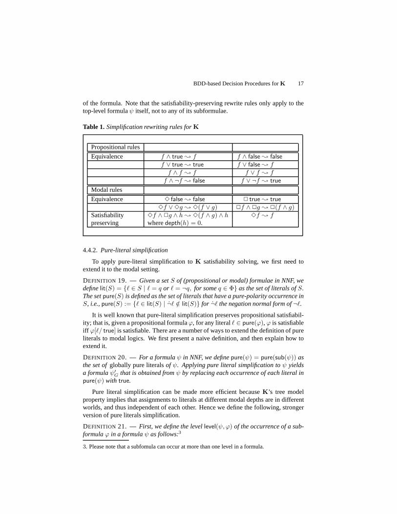
4.4.1. Rewrite rules
Our preprocessing includes rewriting according to the rewrite rules given in Ta-ble 1. It is easy to see that the rules are equivalence or satisfiability preserving. Theserules by themselves are only modestly effective forK formulae; they do become quiteeffective, however, when implemented in combination with pure-literal simplification,described below. These rules allows us to propagate the effects of pure-literal simplifi-cation by removing redundant portions of the formula after pure-literal simplification.This usually allows more pure literals to be found and can greatly reduce the size
BDD-based Decision Procedures forK 17
of the formula. Note that the satisfiability-preserving rewrite rules only apply to thetop-level formulaψ itself, not to any of its subformulae.
Table 1. Simplification rewriting rules forK
Propositional rules
Equivalence f ∧ true ; f f ∧ false ; false
f ∨ true ; true f ∨ false ; ff ∧ f ; f f ∨ f ; f
f ∧ ¬f ; false f ∨ ¬f ; true
Modal rules
Equivalence 3 false ; false 2 true ; true
3f ∨ 3g ; 3(f ∨ g) 2f ∧ 2g ; 2(f ∧ g)Satisfiability 3f ∧ 2g ∧ h ; 3(f ∧ g) ∧ h 3f ; fpreserving wheredepth(h) = 0.
4.4.2. Pure-literal simplification
To apply pure-literal simplification toK satisfiability solving, we first need toextend it to the modal setting.
DEFINITION 19. — Given a setS of (propositional or modal) formulae in NNF, wedefinelit(S) = {ℓ ∈ S | ℓ = q or ℓ = ¬q, for someq ∈ Φ} as the set of literals ofS.The setpure(S) is defined as the set of literals that have a pure-polarity occurrence inS, i.e.,pure(S) := {ℓ ∈ lit(S) | ¬̇ℓ /∈ lit(S)} for ¬̇ℓ the negation normal form of¬ℓ.
It is well known that pure-literal simplification preservespropositional satisfiabil-ity; that is, given a propositional formulaϕ, for any literalℓ ∈ pure(ϕ), ϕ is satisfiableiff ϕ[ℓ/ true] is satisfiable. There are a number of ways to extend the definition of pureliterals to modal logics. We first present a naive definition,and then explain how toextend it.
DEFINITION 20. — For a formulaψ in NNF, we definepure(ψ) = pure(sub(ψ)) asthe set ofglobally pure literalsof ψ. Applying pure literal simplification toψ yieldsa formulaψ′
G that is obtained fromψ by replacing each occurrence of each literal inpure(ψ) with true.
Pure literal simplification can be made more efficient because K’s tree modelproperty implies that assignments to literals at differentmodal depths are in differentworlds, and thus independent of each other. Hence we define the following, strongerversion of pure literals simplification.
DEFINITION 21. — First, we define the levellevel(ψ, ϕ) of the occurrence of a sub-formulaϕ in a formulaψ as follows:3
3. Please note that a subfomula can occur at more than one levelin a formula.

18 JANCL – -/2006. Special Issue on Implementation of Logics
– If ψ = ϕ, thenlevel(ψ, ϕ) = 0;
– If ϕ = ϕ′∧ϕ′′,ϕ′∨ϕ′′, or ¬ϕ′, thenlevel(ψ, ϕ′) = level(ψ, ϕ′′) = level(ψ, ϕ);
– If ϕ = 2ϕ′ or 3ϕ′, thenlevel(ψ, ϕ′) = level(ψ, ϕ) + 1.
For ψ in NNF, we definelevel-pure literalsby purei(ψ) = pure(subi(ψ)), for0 ≤ i ≤ depth(ψ), and we defineψ[purei(ψ)/ true]i to be the result of substitut-ing each occurrence at leveli of a literal in purei(ψ) with true. Applying level-wise pure literal simplification toψ yields a formulaψ′
L = ψ[pure0(ψ)/ true]0 . . .[puredepth(ψ)(ψ)/ true]depth(ψ).
It is possible to push this idea of “separation” further. Because each world in themodel may satisfy a different subset of formulae, if a literal occurs both positively andnegatively at leveli inside a diamond subformula, then we still might replace it withtrue whilst preserving satisfiability. However, checking whether a subformula may besubstituted withtrue then involves such a huge overhead that we do not believe thatitjustifies its implementation.
We now prove that pure-literal simplification preserves satisfiability.
THEOREM 22. — Letψ be in NNF. Thenψ is satisfiable iffψ′G is satisfiable iffψ′
L issatisfiable.
PROOF. — We writeψ′ instead ofψ′G orψ′
L, when the formula used is clear from thecontext. First, we show that substituting a single pure literal ℓ preserves satisfiability.Theorem 22 follows then by induction on the number of pure literals.
The only-if direction is due to the fact that the2 and3 operators aremonotone[BLA 01]. More precisely, letψ be a formula in NNF,α a subformula occurrence ofψ, andβ a formula that is logically implied byα, thenψ[α/β] is logically implied byψ. Since everyℓ impliestrue, satisfiability ofψ implies satisfiability ofψ′.
For the if direction, letK ′ = 〈Φ,W,R,L′〉 be a finite tree Kripke structures ofdepthdepth(ψ) with w0 ∈ W the root of the tree andK ′, w0 |= ψ′.
– Globally pure literals, i.e., ψ′ = ψ′G. Since ℓ does not occur inψ′
G, wecan assume thatL′ does not define a truth value forℓ. We construct a modelK = 〈Ψ,W,R,L〉 from K ′ by takingL to be the following extension ofL′: ifℓ ∈ AP , thenL(ℓ) = W , otherwiseℓ = ¬q for someq ∈ AP and we setL(q) = ∅. We claim that, for every worldw ∈ W and every formulaϕ ∈ sub(ψ),K ′, w |= ϕ[ℓ/ true] impliesK,w |= ϕ.
This claim is an immediate consequence of the fact that, for all w ∈ W ,K,w |= ℓ.
– Level-pure literals: AssumeK ′, w0 |= ψ′, and consider the occurrence ofℓ in ψat leveli. For 0 ≤ i ≤ depth(ψ), letWi = {w | distance betweenw andw0 = i}.We constructK fromK ′ by definingL as follows: (1)L(q) = L′(q) for eachq that isnot the proposition inℓ. (2)L(q) ∩Wj = L′(q) ∩Wj for eachj 6= i, (3) if ℓ ∈ AP ,then setL(ℓ) ∩Wi = Wi, otherwise setL(q) ∩Wi = ∅ whenℓ = ¬q.
For eachϕ ∈ subi(ψ) andw ∈ Wi, we have thatK ′, w |= ϕ[ℓ/ true]d−i impliesK,w |= ϕ. This is an immediate consequence of the fact that, for allw ∈ Wi,
BDD-based Decision Procedures forK 19
K,w |= ℓ. SinceK andK ′ coincide on the interpretation of all propositional variablesin worlds inW \Wi, and on the interpretation of all propositional variables differentfromAP (ℓ) in all worlds, it follows thatK,w0 |= ψ[ℓ/ true]d.
■
5. Implementation
In this section, we describe how to implement our algorithmsand their variationsusing Binary Decision Diagrams (BDDs).
5.1. Base algorithms
We use Binary Decision Diagrams (BDDs) [BRY 86, AND 98] to represent setsof types. BDDs, or more precisely, Reduced Ordered Binary Decision Diagrams(ROBDDs), are obtained from binary decision trees by following a fixed variablesplitting order and by merging nodes that have identical child-diagrams. BDDs pro-vide a canonical representation for Boolean functions. Experience has shown thatBDDs often provide a very compact representation for very large Boolean functions,and that various operations on Boolean functions can be carried out efficiently ontheir BDD representation. Consequently, over the last decade, BDDs have had adramatic impact in the areas of synthesis, testing, and verification of digital sys-tems [BEE 94, BUR 92].
In this section, we describe how our two basic algorithms, top-down and bottom upwith types, are implemented using BDDs. First, we define abit-vector representationof types. Since types are complete in the sense that either a subformula or its negationmust belong to a type, it is possible for a formula and its negation to be representedusing a single BDD variable.
The representation of typesa ⊆ cl(ψ) as bit vectors is defined as follows: first, wesplit cl(ψ) into positive and negative formulae, i.e.,
cl+(ψ) := {ϕi ∈ cl(ψ) | ϕi is not of the form¬ϕ′} andcl−(ψ) := {¬ϕ | ϕ ∈ cl+(ψ)},
and we usem for | cl+(ψ)| = | cl(ψ)|/2. Then, forcl+(ψ) = {ϕ1, . . . , ϕm}, a vector~a = 〈a1, . . . , am〉 ∈ {0, 1}m represents the set4 a ⊆ cl(ψ) with ϕi ∈ a iff ai = 1.
A set of such bit vectors can obviously be represented using aBDD with m vari-ables. It remains to “filter out” those bit vectors that represent types.
We defineconsistentψ as the characteristic predicate for types:consistentψ(~a) =∧
1≤i≤m consistentiψ(~a), whereconsistentiψ(~a) is defined as follows:
4. Please note that this set is not necessarily a type.
20 JANCL – -/2006. Special Issue on Implementation of Logics
– if ϕi is neither of the formϕ′ ∧ ϕ′′ norϕ′ ∨ ϕ′′, thenconsistentiψ(~a) = 1,
– if ϕi = ϕ′ ∧ ϕ′′, thenconsistentiψ(~a) = (ai ↔ (a′ ∧ a′′)), wherea ↔ b is theusual shorthand for(a ∧ b) ∨ (¬a ∧ ¬b),
– if ϕi = ϕ′ ∨ ϕ′′, thenconsistentiψ(~a) = (ai ↔ (a′ ∨ a′′)),
wherea′ = aℓ if ϕ′ = ϕℓ ∈ cl+(ψ), anda′ = ¬aℓ if ϕ′ = ¬ϕℓ for ϕℓ ∈ cl+(ψ),anda′′ = ak if ϕ′′ = ϕk ∈ cl+(ψ), anda′′ = ¬ak if ϕ′′ = ¬ϕk for ϕk ∈ cl+(ψ).
From this, the implementation ofInit is fairly straightforward: For the top-downalgorithm,
Init(ψ) := {~a ∈ {0, 1}m | consistentψ(~a)},
and for the bottom-up algorithm,
Init(ψ) := {~a ∈ {0, 1}m | consistentψ(~a) ∧∧
ϕi=2ϕ′
ai}.
In the following, we do not distinguish between a type and itsrepresentation as abit vector~a. Next, to specifybad(·) andsupp(·), we define auxiliary predicates:
– 31,i(~x) is read as “~x needs a witness for a diamond operator at positioni” andis true iff xi = 0 andϕi = 2ϕ′.
– 32,i(~y) is read as “~y is a witness for a negated box formula at positioni” and istrue iff ϕi = 2ϕj andyj = 0 orϕi = 2¬ϕj andyj = 1 for ϕj ∈ cl+(ψ).
– 21,i(~x) is read as “~x requires support for a box operator at positioni” and is trueiff xi = 1 andϕi = 2ϕ′.
– 22,i(~y) is read as “~y provides support for a box operator at positioni” and istrue iff ϕi = 2ϕj andyj = 1 orϕi = 2¬ϕj andyj = 0 for ϕj ∈ cl+(ψ).
For a setA of types, we construct the BDD that represents the “maximal”accessi-bility relation∆, i.e., a relation that includes all those pairs(~x, ~y) such that~y supportsall of ~x’s box formulae. For types~x, ~y ∈ {0, 1}m, we define
∆(~x, ~y) =∧
1≤i≤m
(21,i(~x) → 22,i(~y)).
Given a setA of types, we write the corresponding characteristic function asχA, andwe useχA for the characteristic function of the complement ofA. Next, we show howto implement the top-down and the bottom-up algorithm usingthe predicatesχA, ∆,3j,i, and2j,i.
For the top-down approach, the predicatebad is true on those types that containa negated box formula which is not witnessed in the current set of types. Thus, for anegated box formulaϕi = ¬2ϕj , we define the predicatebadi as follows:
χbadi(X)(~x) = 31,i(~x) ∧ ∀~y : ((χX(~y) ∧ ∆(~x, ~y)) → ¬32,i(~y)),
BDD-based Decision Procedures forK 21
and thusbad(X) can be written as
χbad(X)(~x) =∨
1≤i≤m
χbadi(X)(~x).
In our implementation, we compute eachχbadi(X) and use it in the implementation of
the top-down and the bottom-up algorithm. It is easy to see thatχbadi(X) is equivalent
to31,i(~x) → ∃~y : (χX(~y) ∧ ∆(x, y) ∧ 32,i(~y)).
For the top-down algorithm, theUpdate function can be written as:
χX\bad(X)(~x) := χX(~x) ∧∧
1≤i≤m
(χbadi(X)(~x))
For the bottom-up algorithm, we must take care to only add bitvectors representingtypes, and so theUpdate function can be implemented as:
χX∪supp(X)(~x) := χX(~x) ∨ (χconsistentψ (~x) ∧∧
1≤i≤m
(χbadi(X)(~x))
These functions can be written more succinctly using the pre-image function for therelation∆:
preim∆(χN )(~x) = ∃~y : χN (~y) ∧ ∆(~x, ~y).
Using pre-images, we can rewriteχbadi(X) as follows:
χbadi(X)(~x) = 31,i(~x) → preim∆(λ(~x).χX(~x) ∧ 32,i(~x))(~x).
Finally, the bottom-up algorithms can be implemented as iterations over the setsχX∪supp(X), and the top-down algorithms can be implemented as iterations over thesetsχX\bad(X) until a fixpoint is reached. Then checking whetherψ is present in atype of this fixpoint is trivial.
The pre-image operation is a key operation in both the bottom-up and the top-down approaches. It is also known to be a key operation in symbolic model checking[BUR 92] and it has been the subject of extensive research (cf. [BUR 91, GEI 94,RAN 95, CIM 00]) since it can be a quite time and space consuming operation. Vari-ous optimizations can be applied to the pre-image computation to reduce the time andspace requirements. A method of choice is that ofconjunctive partitioningcombinedwith early quantification. The idea is to avoid building a monolithic BDD for the rela-tion ∆, since this BDD can be quite large. Rather, we take advantageof the fact that∆is defined as a conjunction of simple conditions, namely one for each box subformula.Thus, to compute the pre-imagepreim∆, we have to evaluate a quantified Booleanformula of the form∃y1 . . . ∃yn(c1 ∧ . . . ∧ cm), where thecis are Boolean formulae.
22 JANCL – -/2006. Special Issue on Implementation of Logics
Suppose, however, that the variableyj does not occur in the clausesci+1, . . . , cm.Then the formula above can be rewritten as
∃y1 . . . ∃yj−1∃yj+1 . . . ∃yn(∃yj(c1 ∧ . . . ∧ ci)) ∧ (ci+1 ∧ . . . ∧ cm).
This enables us to apply existential quantification to smaller BDDs.
Of course, there are many ways in which one can cluster and re-order thecis.One way we used is the methodology developed in [RAN 95], called the “IWLS 95”methodology, to compute pre-images. We have also tried other clustering mecha-nisms, namely the “bucket-elimination” approach described in [San 01]. Given a setof conjunctive componentsc1, . . . , cn, we first compute the variable support set foreach component asY1, . . . , Yn. Then, a graph of interference of variables is con-structed: every vertex represents a variable, and there is an edge between variablesyiandyj if yi andyj occur together in someYk. We conduct a “maximum cardinalityordering” of the variables, after whichy1 is the variable that occurs with the maximalnumber of edges, andyi has the maximum number of edges intoy1, . . . , yi−1. Givensuch a variable order, we can order the conjunctive components in the order of the firstoccurrence of the highest (or lowest) ordered variables (either forward or backward).We have implemented all four combinations in this case, but it will turn out that theperformance improvements are minimal.
5.2. Optimizations
5.2.1. Particles
The encoding of the particle-based approach with BDDs is analogous to the en-coding of the type-based approach. Since the consistency requirement for particles ismore relaxed than that of types, each subformula insub(ψ) (also the negated ones) isrepresented by a variable. Givensub(ψ) = {ϕ1, ...ϕn}, a vector~p = 〈p1, ...pn〉 ∈{0, 1}n represents a setp ⊆ sub(ψ) with ϕi ∈ p iff pi = 1.
Then, as for types, we define a characteristic predicate for particle vectorsconsistentψ(~p) := ∧1≤i≤n consistentiψ(~p), whereconsistentiψ(~p) is defined as fol-lows:
– if ϕi is neither of the formϕj ∧ ϕk norϕj ∨ ϕk, thenconsistentiψ(~p) = 1,
– if ϕi = ϕj ∧ ϕk, thenconsistentiψ(~p) = (pi → (pj ∧ pk)),
– if ϕi = ϕj ∨ ϕk, thenconsistentiψ(~p) = (pi → (pj ∨ pk)), and
– if ϕi = ¬ϕj , thenconsistentiψ(~p) = ¬(pi ∧ pj).
Finally, we update the auxiliary predicates for particles:
– 31,i(~x) is true iff xi = 1 andϕi = 3ϕ′,
– 32,i(~y) is true iffϕi = 3ϕj andyj = 1,
– 21,i(~x) is true iff xi = 1 andϕi = 2ϕ′ (the same as for types), and

BDD-based Decision Procedures forK 23
– 22,i(~y) is true iffϕi = 2ϕj andyj = 1.
No other predicate changes, in particularpreim andbad do not change.
5.2.2. Lean vector approaches
Lean approaches have much more relaxed consistency predicates at the cost ofbigger witness/support predicates. For lean approaches, we first need to define a con-sistency requirement for lean vectors. In the consistency requirement, only the con-straints inconsistentiψ(~x) that is related to thoseϕi in atom(ψ) (Note for the particlecase the consistency requirement is empty) are used.
In contrast, the auxiliary (witness/support) predicate for the lean approach is sig-nificantly more complex. We now define the corresponding auxiliary functions forlean assignments.
For lean types and lean particles,31,i and21,i are the same as for full types andparticles. However, since the subformula occurring insidea modal operator may bea Boolean combination, we need to redefine the functions32,i, 22,i with the sameintuition as for full type and particle vectors. To do this, we first define the auxiliaryfunctionstripi as follows:
strip i(~y) =
stripj(~y) ∧ stripk(~y) if ϕi = ϕj ∧ ϕkstripj(~y) ∨ stripk(~y) if ϕi = ϕj ∨ ϕk¬ stripj(~y) if ϕi = ¬ϕjyi if ϕi ∈ atom(ψ) for types orpart(ψ) for particles
Obviously, for both lean types and lean particles ,stripi can be computed when parsingthe input formula, and be kept in a table.
Next,32,i and22,i can be defined as follows:
32,i(~y) =
stripj(~y) for particles, ifϕi = 3ϕj¬ stripj(~y) for types, ifϕi = 2ϕj with ϕj ∈ cl+(ψ)stripj(~y) for types, ifϕi = 2¬ϕj with ϕj ∈ cl+(ψ)
22,i(~y) =
stripj(~y) for particles, ifϕi = 2ϕjstripj(~y) for types, ifϕi = 2ϕj with ϕj ∈ cl+(ψ)¬ stripj(~y) for types, ifϕi = 2¬ϕj with ϕj ∈ cl+(ψ)
Again, all other predicates such aspreim andbad do not change.
5.2.3. Level-based evaluation
The level-based evaluation approaches are computed in a similar way. However,since all levels are treated separately, at each level, we only need to consider thoseunwitnessed box formulae of that level—before, we had to consider all possibly un-witnessed negated box formulae—which leads to the relativized predicatebadj(X).

24 JANCL – -/2006. Special Issue on Implementation of Logics
Similarly, to test whether a given vector indeed representsa type, the constraint pred-icateconsistentiψ for the level-based approach only needs to consider subformulae ofthe same leveli. So, we can relativize both the lean and the full variant of the typeapproach by definingχleveli(X) as follows:
χleveli(X)(~x) = χconsistentiψ(~x) ∧
∧
{j|ϕj∈cli(ψ)}
(χbadj(X)(~x)).
Then we can specify the level-based variants by settingχIniti(~a) = consistenti(~a)andχUpdate(A,i)(~a) = χconsistenti(~a) ∧ χleveli(A)(~a).
The level-based evaluation for particles can be implemented in the same way byreplacingcli with subi and relativizing the corresponding predicates for particles.
5.3. Variable ordering
It is well-known that the performance of BDD-based algorithms is very sensitiveto BDD variable order since it is a primary factor influencingBDD size [BRY 86].In our experiments, a major factor in performance degradation is space blow-ups ofBDDs, including the intermediate BDDs computed during pre-image operation. In allour algorithms, however, every step in the REPEAT loop uses BDDs with variablesfrom different modal depth, and thus dynamic variable ordering is of limited benefitfor KBDD (though it is necessary when dealing with intermediate BDD blowups)because there may not be sufficient reuse to make it worthwhile. Thus, we focusedhere on heuristics to construct a good initial variable order, i.e., one that is appropriatefor KBDD. In this, we follow the work of Kamhi and Fix [KAM 98a] who argued infavor of application-dependent variable order. As we show in Section 7.1.5, choosinga good initial variable order does improve performance, butthe improvement is rathermodest.
A naive method for assigning an initial variable order to a set of subformulaewould be to traverse the syntax DAG of the input formula5 in some order. We used adepth-first, pre-order traversal. This order, however, does not meet the basic principleof BDD variable ordering, which is to keep related variablesin close proximity. Ourheuristic is aimed at identifying such “close” variables. We found that related variablescorrespond to subformulae that are related via the “sibling” or “niece” relationships.More precisely, we say thatvx is achild of vy if, for the corresponding subformulae,we have thatϕx ∈ subi(ψ), ϕy ∈ subi+1(ψ), andϕy is a subformula ofϕx, for some0 ≤ i < depth(ψ).6 We say thatvx andvy aresiblingsif either bothϕx andϕy arein subi(ψ) or they are both children of another variablevz . We say thatvy is anieceof vx if there is a variablevz such thatvz is a sibling ofvx andvy is a child ofvx.We say thatvx andvy aredependentif they are related via the sibling or the niece
5. The syntax DAG is obtained from the syntax tree of a formula by identifying nodes labeledwith the same subformula.6. For the type approach,subi has to be replaced withcli accordingly.
BDD-based Decision Procedures forK 25
relationship. The rationale is that we want to optimize state-set representation forpre-image operations. Keeping siblings close helps in keeping state-set representationcompact. Keeping nieces close to their “aunts”, helps in keeping intermediate BDDscompact.
Our heuristics builds a variable order from the root of the formula DAG down.We start with left-to-right traversal order of top variables in the parse tree ofψ as theorder for variables corresponding to subformulae insub0(ψ). Given an order of thevariables of modal depth< i, a greedy approach is used to determine the placementof variables at modal depthi. When we insert a new variablev, we measure thecumulative distance ofv from all variables already in the order that are dependenton v, and choose a location forv that minimizes the cumulative distance from otherdependent variables. We refer to this approach as thegreedyapproach, as opposed tothenaiveapproach of depth-first pre-order.
6. Reducing K to QBF
BothK and QBF have PSPACE-complete satisfiability problems [LAD 77, STO 77],and thus these two problems are polynomially reducible to each other. A naturalreduction from QBF toK is described in [HAL 92]. In the last few years, exten-sive effort was carried out into the development of highly-optimized QBF solvers[GIU 01, CAD 99, LET 02]. One motivation for this effort is thehope of using QBFsolvers as generic search engines [RIN 99], much is the same way that SAT solversare being used as generic search engines, cf. [BIE 99]. This suggests that we can re-alistically hope to decideK satisfiability by using a natural reduction ofK to QBF,and then applying one of the highly optimized QBF solvers. Such an approach is sug-gested in [CAD 99] without providing either details or results. Next, we describe sucha reduction, and evaluate it empirically in the next section, together with ourKBDDalgorithms.
QBF is an extension of propositional logic with quantifiers.The set of QBF for-mulae is constructed from a setΦ = {x1, . . . xn} of Boolean variables, and closedunder the Boolean connectives∧ and¬, as well as the quantifier∀xi. As usual, weuse other Boolean operators as abbreviations, and∃xi.ϕ as shorthand for¬∀xi.¬ϕ.Like propositional formulae, QBF formulae are interpretedover truth assignmentsτ : Φ −→ {1, 0}. The semantics of quantifiers is defined as usual for the Booleanpart, and as follows for the quantifiers:τ |= ∀p.ϕ iff τ [p/0] |= ϕ andτ [p/1] |= ϕ,whereτ [p/i] is obtained fromτ by settingτ(p) := i.
By Theorem 18, aK formulaψ of modal depthd is satisfiable iff there existsa sequenceP = 〈P0, P1, . . . , Pd〉 of particle sets (satisfying the conditions formu-lated in Section 4.3) such thatψ ∈ p for somep ∈ P0. We construct QBF formulaef0, f1, . . . fd so that eachfi encodes the particle setPi. The construction is by back-ward induction fori = d . . . 0. For everyϕ ∈ subi(ψ), we have a correspondingvariablexϕ,i as a free variable infi. Then, for eachp ⊆ subi(ψ), we define the

26 JANCL – -/2006. Special Issue on Implementation of Logics
truth assignmentτ ip as follows: τ ip(xϕ,i) = 1 iff ϕ ∈ p. The intention is to havePi = {p ⊆ subi(ψ)|τ ip |= fi}. We then say thatfi characterizesPi.
To definefi, we need some notation: we useparticlei(ψ) for the set of all con-sistent particle vectors ofsubi(ψ). We start by constructing a propositional formulalci such that, for eachp ⊆ subi(ψ) we have thatp ∈ particlei(ψ) iff τ ip |= lci. Theformulalci is a conjunction of clauses as follows:
– Forϕ = ¬ϕ′ ∈ subi(ψ), we have the clausexϕ,i → ¬xϕ′,i.
– Forϕ = ϕ′∧ϕ′′ ∈ subi(ψ), we have the clausesxϕ,i → xϕ′,i andxϕ,i → xϕ′′,i.
– Forϕ = ϕ′ ∨ ϕ′′ ∈ subi(ψ), we have the clausexϕ,i → (xϕ′′,i ∨ xϕ′′,i).
For i = d we simply setfd := lcd. Indeed, we havePd = particled(ψ) = {p ⊆subd(ψ) | τdp |= fd}. Thus,fd characterizesInitd(ψ).
For i < d, suppose we have already constructed a QBF formulafi+1 that char-acterizesPi+1. We start by constructingf ′
i , which also characterizesPi, but usesexponential size for better readability. Later, we will present an equivalentfi whichuses the power of alternation to compressf ′
i . We setf ′d = fd and
f ′i := lci ∧
∧
3ϕ∈subi(ψ)
mc3ϕ,
wheremc3ϕ ensures that, if3ϕ is in a particlep ∈ Pi, then3ϕ in p is witnessed bya particle inPi+1. That is, forsubi+1(ψ) = {θ1, . . . , θki+1
}, we set
mc3ϕ := x3ϕ,i → ∃xθ1,i+1 . . . ∃xθki ,i+1(fi+1 ∧ xϕ,i+1 ∧ tri), wheretri :=
∧
2η∈subi(ψ)[x2η,i → xη,i+1].
LEMMA 23. — If f ′i+1 characterizesPi+1, thenf ′
i characterizesPi = Update(Pi+1, i).
PROOF. — By construction,lci characterizesparti(ψ). For the witnessing require-ment, we can see that, ifτ ip |= mc3ϕ andx3ϕ,i, then there is an assignmentτ i+1
p′
whereτ ip ∪ τi+1p′ |= f ′
i+1 ∧xϕ,i+1 ∧ tri. This is equivalent to asserting thatp′ ∈ Pi+1,ϕ ∈ p′ andRi(p, p′). ■
COROLLARY 24. — ψ is satisfiable iff∃xθ1,0 . . .∃xθk0 ,0xψ,0 ∧ f′0 is satisfiable.
PROOF. — The claim follows from the soundness and completeness ofKBDD. ■
This reduction ofK to QBF is correct; unfortunately, it is not polynomial. Theproblem is thatf ′
i requires a distinct copy offi+1 for each formula3ϕ in subi(ψ).This may cause an exponential blow-up forf ′
0. To constructfi which uses only asingle copy offi+1, we replace the conjunction over all3ϕ formulae insubi(ψ) bya universal quantification. Letk be an upper bound on the number of3ϕ formulae insubi(ψ), for 0 ≤ i ≤ depth(ψ). We associate an indexj ∈ {0, . . . , k − 1} with eachsuch subformula; thus, we letξij the j-th 3ϕ subformula insubi(ψ), in which case
BDD-based Decision Procedures forK 27
we denoteϕ by strip(ξij). Letm = ⌈log(k)⌉. We introducem new Boolean variablesy1, . . . , ym. Each truth assignment to the variablesyi represents a number between0 andk in binary coding, and we refer to this number byval(y) and use it to referto 3 subformulae. Letwitnessi be the formula
∨k−1j=0 xξij , which asserts that some
witnesses are required.
Using this notation, we can now writefi in a compact way:
lci ∧ ∀y1, . . . ,∀ym : ∃xθ,i+1:{θ∈subi+1(ψ)} : witnessi →
fi+1 ∧ tri ∧k−1∧
j=0
((val(y) = j ∧ xξij,i) → xstrip(ξi
j),i+1)
.
The formulafi first asserts the local consistency constraintlci. The quantification ony1, . . . , ym simulates the conjunction on allk 3 subformulae insubi(ψ). We thencheck ifwitnessi holds, in which case we assert the existence of the witnessing par-ticle. We usefi+1 to ensure that this particle is inPi+1 andtri to ensure satisfactionof 2 subformulae. Finally, we letval(y) point to the3 subformulae that needs to bewitnesses. Note thatfi contains only one copy offi+1.
LEMMA 25. — fi andf ′i are logically equivalent.
As an immediate consequence of the above lemma and Corollary24, we obtainthe following result.
COROLLARY 26. — ψ is satisfiable iff∃xθ1,0 . . .∃xθk0 ,0xψ,0 ∧ f0 is satisfiable.
Analogously to our other approaches, this approach can be optimized further byreducing redundancy, i.e., by restricting variables to those representing non-Booleansubformulae. We implemented this optimization and report on our experiments in thenext section.
7. Experimental Results
In this section, we report on our empirical evaluation of thealgorithms describedthroughout this paper and their optimizations. We first report on comparisons betweenthe variousKBDD algorithms and analyze the effects of the different optimizationsand the influence of variable ordering. This allows us to determine the “best” config-uration for ourKBDD approach. Secondly, we compare this bestKBDD algorithmwith otherK solvers and with an implementation of the translation into QBF methoddescribed in the previous section.
We implemented the BDD-based decision procedure and its variants in C++ usingthe CUDD 2.3.1 [SOM 98] package for BDDs, and we implemented formula simpli-fication preprocessor in OCaml. The parser for the languagesused in the benchmarksuites are taken with permission from *SAT [TAC 99].7
7. All tests were run on a Pentium 4 1.7GHz with 512MB of RAM, running Linux kernelversion 2.4.2. The solver is compiled with gcc 2.96 with parts in OCaml 3.04.
28 JANCL – -/2006. Special Issue on Implementation of Logics
7.1. Comparing theKBDD variants
To analyze the usefulness of each optimization techniques used, we run the algo-rithm with different optimization configurations on theK part of TANCS 98 [HEU 96]and the MODAL PSPACE division of TANCS 2000 [MAS 00]. Both aresuites of scal-able benchmarks which contain both provable and non-provable formulae. In TANCS98, simple formulae have their difficulty increased by re-encoding them with superflu-ous subformulae. In TANCS 2000, formulae are constructed bytranslating QBF for-mulae intoK using three translation schemes, namely the Schmidt-Schauss-Smolkatranslation, which gives easy formulae, the Ladner translation, which gives mediumdifficulty formulae, and the Halpern translation, which gives hard formulae. TANCS98 provides more “easy” formulae, and we used it to provide a clearer picture in casethat the unoptimized algorithms took too long on TANCS 2000.To get a clearer pic-ture and a guideline, each test was also run with *SAT, and we limited the memoryavailable for BDDs to 384MB and the time to 1000s.
7.1.1. The basic algorithms
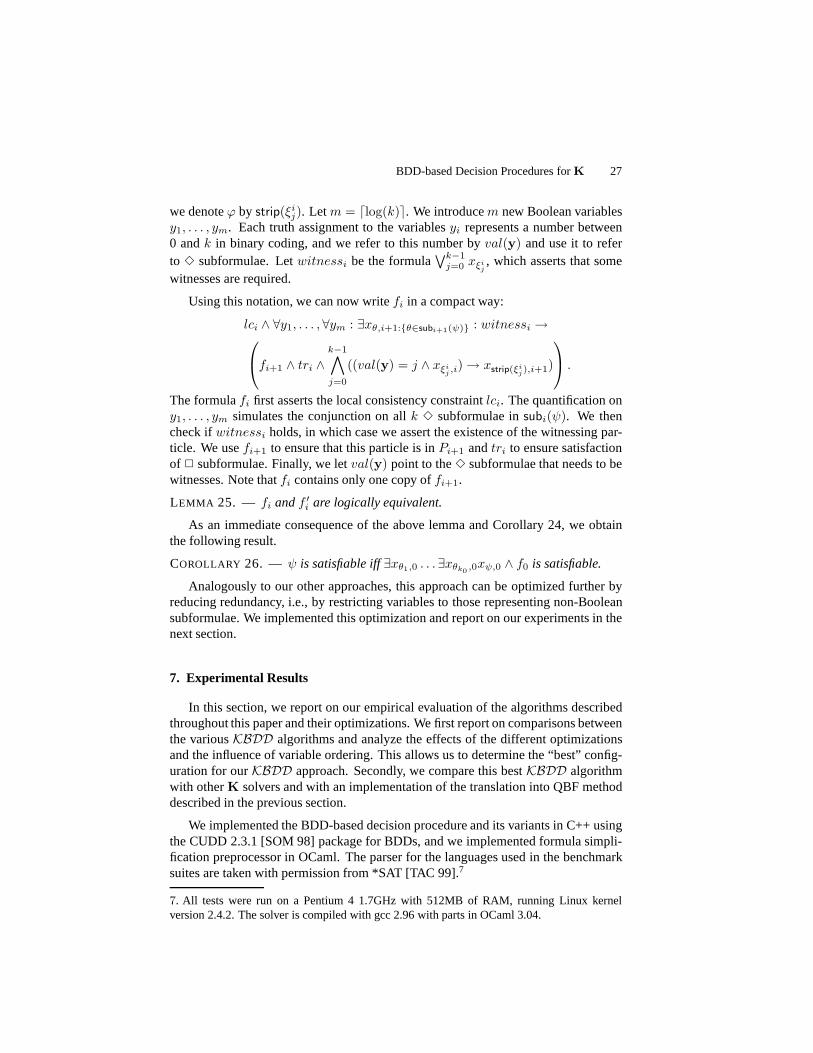
To compare our basic algorithms, top-down and bottom-up using full types, werun them both on TANCS 98. The results are presented in Fig. 1.We compare thenumber of cases solved by each of the algorithms under a certain time limit, so the“better” solver is the one that solved more problem instances. We can see that *SATclearly outperforms our two basic algorithms. A reason for this “weak” behaviorof our approaches is that the intermediate results of the pre-image operation are solarge that the we ran out of memory. The difference between top-down and bottom-up approaches is minor. Top-down slightly outperforms bottom-up since top-downremoves types, which only requires the consistency requirement to be asserted oncebefore iteration, while bottom-up adds types, which requires an extra conjunction toensure only consistent types are added.
101
102
103
104
105
106
0
50
100
150
200
250
300
350
Running Time (ms)
Cas
es c
ompl
eted
*SATtopdown−full−typebottomup−full−type
Figure 1. Top-down versus bottom-up on TANCS 98
BDD-based Decision Procedures forK 29
7.1.2. Particle approaches
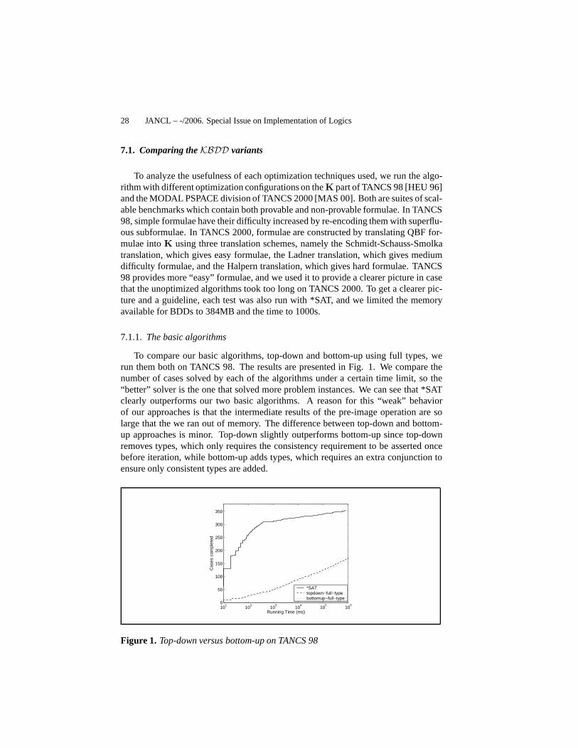
Next, we compare the variants using types with their full particle-based variants.The results are presented in Fig. 2. We can see that, on TANCS 98, the particle ap-proach slightly outperforms the type approach. Most of the improvements come fromthe use of negation normal form, which allows us to distinguish between diamonds andboxes, resulting in a reduction of the number of operations to compute pre-images.
101
102
103
104
105
106
0
50
100
150
200
250
300
350
Running Time (ms)
Cas
es c
ompl
eted
*SATtopdown−full−typetopdown−full−particle
101
102
103
104
105
106
0
50
100
150
200
250
300
350
Running Time (ms)
Cas
es c
ompl
eted
*SATbottomup−full−typebottomup−full−particle
Figure 2. Particles vs. types on TANCS 98
7.1.3. Lean approaches
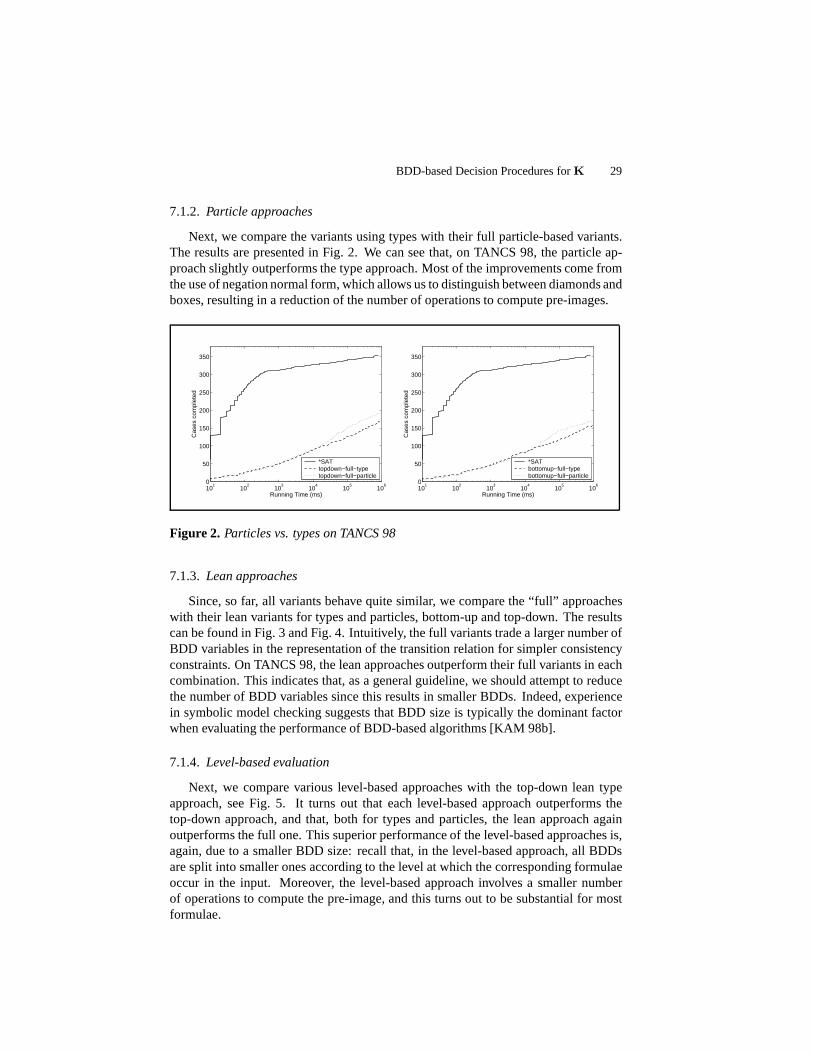
Since, so far, all variants behave quite similar, we comparethe “full” approacheswith their lean variants for types and particles, bottom-upand top-down. The resultscan be found in Fig. 3 and Fig. 4. Intuitively, the full variants trade a larger number ofBDD variables in the representation of the transition relation for simpler consistencyconstraints. On TANCS 98, the lean approaches outperform their full variants in eachcombination. This indicates that, as a general guideline, we should attempt to reducethe number of BDD variables since this results in smaller BDDs. Indeed, experiencein symbolic model checking suggests that BDD size is typically the dominant factorwhen evaluating the performance of BDD-based algorithms [KAM 98b].
7.1.4. Level-based evaluation
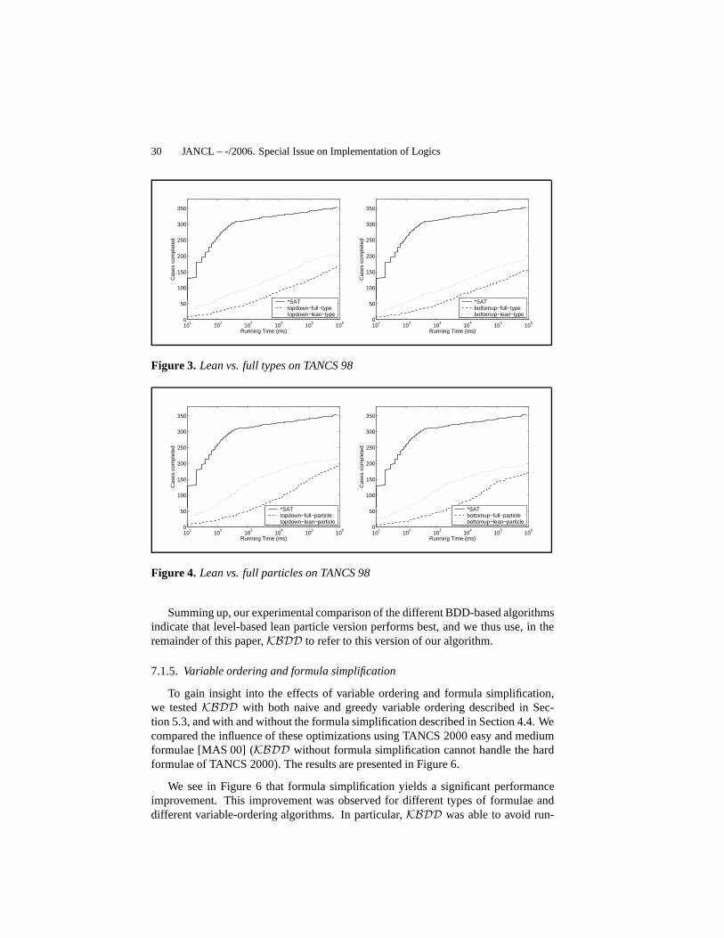
Next, we compare various level-based approaches with the top-down lean typeapproach, see Fig. 5. It turns out that each level-based approach outperforms thetop-down approach, and that, both for types and particles, the lean approach againoutperforms the full one. This superior performance of the level-based approaches is,again, due to a smaller BDD size: recall that, in the level-based approach, all BDDsare split into smaller ones according to the level at which the corresponding formulaeoccur in the input. Moreover, the level-based approach involves a smaller numberof operations to compute the pre-image, and this turns out tobe substantial for mostformulae.
30 JANCL – -/2006. Special Issue on Implementation of Logics
101
102
103
104
105
106
0
50
100
150
200
250
300
350
Running Time (ms)
Cas
es c
ompl
eted
*SATtopdown−full−typetopdown−lean−type
101
102
103
104
105
106
0
50
100
150
200
250
300
350
Running Time (ms)
Cas
es c
ompl
eted
*SATbottomup−full−typebottomup−lean−type
Figure 3. Lean vs. full types on TANCS 98
101
102
103
104
105
106
0
50
100
150
200
250
300
350
Running Time (ms)
Cas
es c
ompl
eted
*SATtopdown−full−particletopdown−lean−particle
101
102
103
104
105
106
0
50
100
150
200
250
300
350
Running Time (ms)
Cas
es c
ompl
eted
*SATbottomup−full−particlebottomup−lean−particle
Figure 4. Lean vs. full particles on TANCS 98
Summing up, our experimental comparison of the different BDD-based algorithmsindicate that level-based lean particle version performs best, and we thus use, in theremainder of this paper,KBDD to refer to this version of our algorithm.
7.1.5. Variable ordering and formula simplification
To gain insight into the effects of variable ordering and formula simplification,we testedKBDD with both naive and greedy variable ordering described in Sec-tion 5.3, and with and without the formula simplification described in Section 4.4. Wecompared the influence of these optimizations using TANCS 2000 easy and mediumformulae [MAS 00] (KBDD without formula simplification cannot handle the hardformulae of TANCS 2000). The results are presented in Figure6.
We see in Figure 6 that formula simplification yields a significant performanceimprovement. This improvement was observed for different types of formulae anddifferent variable-ordering algorithms. In particular,KBDD was able to avoid run-

BDD-based Decision Procedures forK 31
101
102
103
104
105
106
0
50
100
150
200
250
300
350
Running Time (ms)
Cas
es c
ompl
eted
*SATlevel−full−typelevel−lean−typetopdown−lean−type
101
102
103
104
105
106
0
50
100
150
200
250
300
350
Running Time (ms)
Cas
es c
ompl
eted
*SATlevel−full−particlelevel−lean−particletopdown−lean−particle
Figure 5. Level-based evaluation vs. top-down lean approaches on TANCS 98
101
102
103
104
105
106
0
50
100
150
200
Running Time (ms)
Cas
es c
ompl
eted
simp−naivesimp−greedynosimp−naivenosimp−greedy
101
102
103
104
105
106
0
50
100
150
200
Running Time (ms)
Cas
es c
ompl
eted
simp−naivesimp−greedynosimp−naivenosimp−greedy
TANCS 2000 Easy ( nfSSS) TANCS 2000 Medium ( nfLadn)Figure 6. Different optimizations forKBDD on TANCS 2000
ning out of memory in many cases. We can also see that greedy variable ordering isuseful in conjunction with simplification, improving the number of completed casesand sometimes run time as well. Without simplification, the results for greedy vari-able ordering are not consistent: the overhead of finding thevariable order seems tosometimes offset any advantages of applying it.
Summing up, our experiments indicate that the combination of simplification andgreedy variable ordering significantly improves the performance ofKBDD. In the fol-lowing, we will use “optimizedKBDD” to refer to this variant, and we will compareits performance with that of three other solvers.
32 JANCL – -/2006. Special Issue on Implementation of Logics
7.2. ComparingKBDD with other solvers
To assess the effectiveness of BDD-based decision procedures forK, we comparethe optimizedKBDD against three solvers: (1) DLP, which is a tableau-based solver[PAT 99], (2) MSPASS, which is a combination of an optimized translation of modalformulae to first-order formulae and a resolution-based theorem prover [HUS 00]8, (3)K-QBF, which is a combination of our reduction ofK to QBF from Section 24 andthe highly optimized QBF solver semprop [LET 02]. For a fair comparison, we firstchecked for which our simplification optimization is useful, and then used it in thesetwo cases, namely for DLP and K-QBF.
In addition to the formulae from TANCS 98 and TANCS 2000, we also use ran-domly generated formulae, as suggested in [PAT 01]. This scheme generates randommodal-CNF formulae parameterized with the numberN of propositions, the numberK of literals in each clause, the fractionα of modal literals in each clause, the modal-depth boundd, and the numberL of top level clauses.L clauses are generated withKliterals each, whereαK literals are modal and the rest are propositional (the polarityof the literals is chosen uniformly). Each modal literal is expanded into a clause in thesame fashion. The modal depth of the formula is bounded byd. We usedd = [1, 2],K = 3 andα = 0.5 in our experiments. In each experiment,N is fixed and thepropositional complexity of the formula was varied by increasing thedensityL/N .
7.2.1. Results on TANCS suites
In Figure 7 and Figure 8 we see that, on the TANCS 98 benchmarks, DLP outper-forms all other solvers whereas, on the more challenging TANCS 2000 benchmarks,KBDD outperforms the other solvers. The difference betweenKBDD and the othersolvers is most noticeable on the harder portion of the suite, whereKBDD had to usedynamic variable reordering. We take this as an indicator that, indeed, BDD-based ap-proaches may be useful in practice forK satisfiability. MSPASS’s performance couldhave been enhanced by a different choice for its numerous parameters. However, wehave chosen to stick to the setting that worked well for TANCS98 since (a) the currentinvestigation is merely a feasibility study, and (b) findingoptimal parameter settingsfor MSPASS for each experiment would go beyond the scope of this paper. Finally, itturns out that reducingK satisfiability to a search-based QBF solver such as sempropis not a viable approach: this approach was dominated by all other approaches andwas only able to solve a small fraction of the benchmark formulae in TANCS 98. ForTANCS 2000 this approach was so inefficient that we did not report the results.
8. We used MSPASS 1.0.0t1.3 with options -EMLTranslations=2-EMLFuncNary=1 -Select=2-PProblem=0 -PGiven=0 -Sorts=0 -CNFOptSkolem=0 -CNFStrSkolem=0 -CNFRenOps=1 -Split=-1 -Ordering=0 -CNFRenMatch=0 -TimeLimit=1000. Compiler used is gcc-3.1.1 be-cause gcc-2.96 has a serious bug that crashes the resulting executable.

BDD-based Decision Procedures forK 33
101
102
103
104
105
106
0
50
100
150
200
250
300
350
Running Time (ms)
Cas
es c
ompl
eted
KBDDDLPMSPASSK−QBF−Semprop
101
102
103
104
105
106
0
50
100
150
200
Running Time (ms)
Cas
es c
ompl
eted
KBDDDLPMSPASSK−QBF−SempropTANCS 98 TANCS 2000 Easy ( nfSSS)
Figure 7. KBDD vs. DLP, K-QBF and MSPASS on “easy”K formulae
101
102
103
104
105
106
0
50
100
150
200
Running Time (ms)
Cas
es c
ompl
eted
KBDDDLPMSPASS
101
102
103
104
105
106
0
10
20
30
40
50
Running Time (ms)
Cas
es c
ompl
eted
KBDD−reorderDLP
TANCS 2000 Medium ( nfLadn) TANCS 2000 Hard ( nf)Figure 8. KBDD vs. DLP, and MSPASS on more “difficult”K formulae
7.2.2. Results on random modal CNF formulae
More insight into the behavior ofKBDD can be gained by analyzing its behavioron random modal-CNF formulae. The generation of the formulae follows the sugges-tions in [PAT 01]. This scheme generates random modal-CNF formulae parametrizedwith the numberN of propositions, the numberK of literals in each clause, the frac-tionα of modal literals in each clause, the modal-depth boundd, and the numberL oftop level clauses.L clauses are generated withK literals each, whereαK literals aremodal and the rest are propositional (the polarity of the literals is chosen uniformly).Each modal literal is expanded into a clause in the same fashion. The modal depthof the formula is bounded byd. We usedd = 1, 2, K = 3 andα = 0.5 in our ex-periments. In each experimentN was fixed and the propositional complexity of theformula was varied by increasing thedensityL/N .
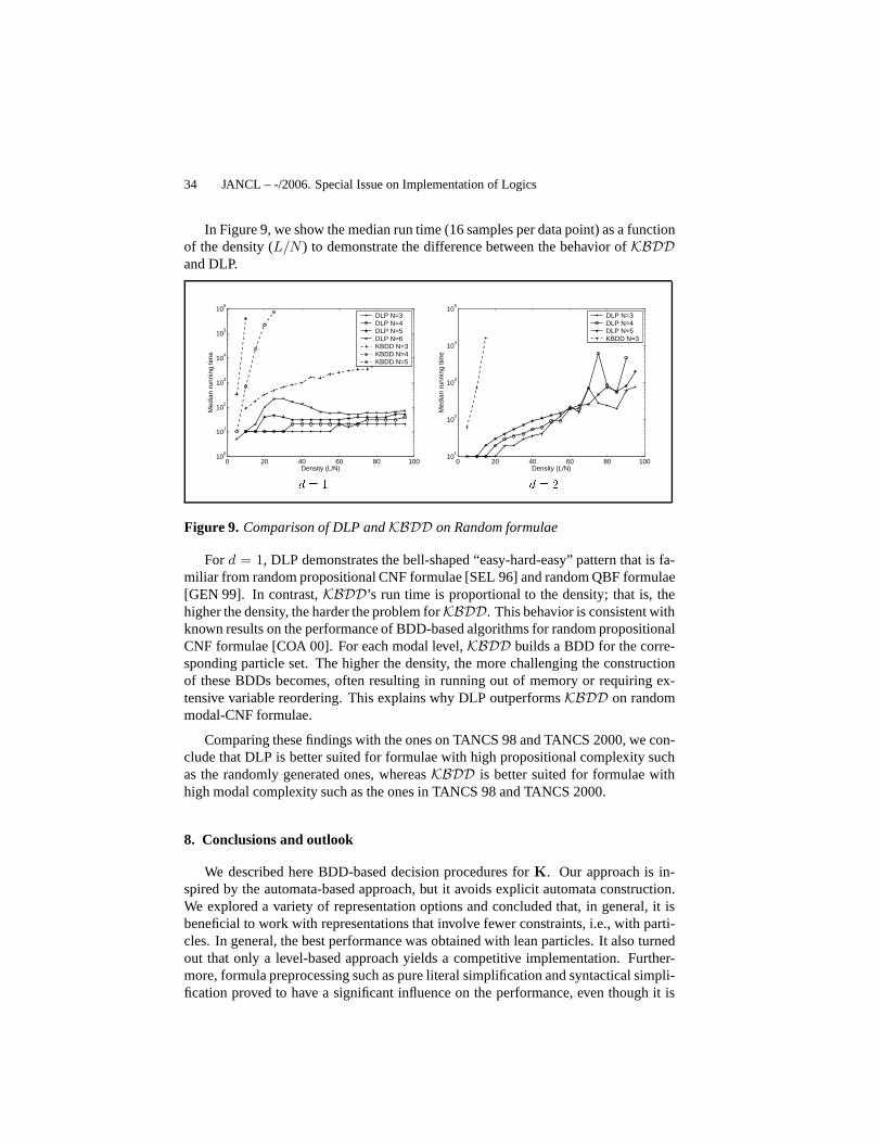
34 JANCL – -/2006. Special Issue on Implementation of Logics
In Figure 9, we show the median run time (16 samples per data point) as a functionof the density (L/N ) to demonstrate the difference between the behavior ofKBDDand DLP.
0 20 40 60 80 10010
0
101
102
103
104
105
106
Density (L/N)
Med
ian
runn
ing
time
DLP N=3DLP N=4DLP N=5DLP N=6KBDD N=3KBDD N=4KBDD N=5
0 20 40 60 80 10010
1
102
103
104
105
Density (L/N)
Med
ian
runn
ing
time
DLP N=3DLP N=4DLP N=5KBDD N=3
d = 1 d = 2Figure 9. Comparison of DLP andKBDD on Random formulae
For d = 1, DLP demonstrates the bell-shaped “easy-hard-easy” pattern that is fa-miliar from random propositional CNF formulae [SEL 96] and random QBF formulae[GEN 99]. In contrast,KBDD’s run time is proportional to the density; that is, thehigher the density, the harder the problem forKBDD. This behavior is consistent withknown results on the performance of BDD-based algorithms for random propositionalCNF formulae [COA 00]. For each modal level,KBDD builds a BDD for the corre-sponding particle set. The higher the density, the more challenging the constructionof these BDDs becomes, often resulting in running out of memory or requiring ex-tensive variable reordering. This explains why DLP outperformsKBDD on randommodal-CNF formulae.
Comparing these findings with the ones on TANCS 98 and TANCS 2000, we con-clude that DLP is better suited for formulae with high propositional complexity suchas the randomly generated ones, whereasKBDD is better suited for formulae withhigh modal complexity such as the ones in TANCS 98 and TANCS 2000.
8. Conclusions and outlook
We described here BDD-based decision procedures forK. Our approach is in-spired by the automata-based approach, but it avoids explicit automata construction.We explored a variety of representation options and concluded that, in general, it isbeneficial to work with representations that involve fewer constraints, i.e., with parti-cles. In general, the best performance was obtained with lean particles. It also turnedout that only a level-based approach yields a competitive implementation. Further-more, formula preprocessing such as pure literal simplification and syntactical simpli-fication proved to have a significant influence on the performance, even though it is
BDD-based Decision Procedures forK 35
not specialized to our method. Finally, we tested various BDD-centric optimizationssuch as clustering with early quantification and initial variable ordering but the effectproved to be rather modest.
We benchmarkedKBDD, our optimized BDD-based solver, against both a nativemodal solver, DLP, and two translation-based solvers, MSPASS and K-QBF. Our re-sults indicate that the BDD-based approach dominates for modally heavy formulae,while search-based approaches dominate for propositionally heavy formulae.
One way to look at the results is thatKBDD, by using a more powerful underly-ing data structure, BDDs, allows the use of a simpler decision procedure. Instead ofrequiring, in the worst case, an exponential number of callsto a propositional satis-fiability procedure,KBDD only requires a polynomial number of calls to BDD op-erations. The natural question arising is, of course, whether such a dependence onthe data structure is reasonable. We know that the complexity of BDD operations ishighly dependent on the size of the BDDs. So, if we are able to control the size of theBDDs, the performance of our decision procedure is acceptable.
Another explanation is that we traded modal complexity for propositional com-plexity. This way, we managed to perform quite well on formulae that only have “big”models. Such formulae are known to cause problems with SAT based solvers. We ob-serve that, on formulae that are satisfiable in “small” models, SAT solvers outperformKBDD. In contrast, on formulae that are only satisfiable in “big” models,KBDD out-performs other SAT solvers. In both cases, the performance of both solvers degradeswith increasing propositional density.
Although our goal was a feasibility study for a BDD-based approach to modalsolvers, and not to develop the “fastestK solver”, theKBDD approach turned outto behave quite well on a considerable number of benchmarks.This is mostly due tothe fact that our approach allowed us to compare and explore the effects of numer-ous optimizations. One obvious optimization technique we did not explore is to avoidthe construction of a monolithic BDD, such as the technique developed for the purelypropositional case [San 01]. Further research is also required to quantify the distinc-tion between “propositionally heavy” and “modally heavy” formulae. This would en-able the development of a combined solver which invokes the appropriate engine forthe formula under test. Another approach would be to developa hybrid solver, com-bining BDD-based and search-based techniques (cf. [GUP 01]for a hybrid approachin model checking), which would perform well on both modallyheavy and proposi-tionally heavy formulae. Finally, we believe that the closerelationship betweenK andQBF can serve as a good starting point for the investigation of novel decision proce-dures for QBF, for example, the quantifier-elimination based solvers Quantor [BIE 04]and QMRES [PAN 04], which use Q-resolution [BUN 95]. We leaveall this for futureresearch.
36 JANCL – -/2006. Special Issue on Implementation of Logics
Acknowledgements
The authors are supported in part by NSF grants CCR-9700061,CCR-9988322,IIS-9908435, IIS-9978135, and EIA-0086264, by BSF grant 9800096, and by a grantfrom the Intel Corporation. The authors would also like to thank the anonymousreviewers for their comments.
9. References
[AND 98] A NDERSEN H., “An Introduction to Binary Decision Diagrams”, report ,1998,Department of Information Technology, Technical University of Denmark.
[ARE 00] ARECESC., GENNARI R., HEGUIABEHEREJ.,DE RIJKE M., “Tree-Based Heuris-tics in Modal Theorem Proving”,Proc. of the 14th Eur. Conf. on Artif. Int., 2000, p. 199-203.
[BAA 01] B AADER F., TOBIES S., “The inverse method implements the automata approachfor modal satisfiability”, report num. LTCS-Report 01-03, 2001, Research group for theo-retical computer science, Aachen university of Technology.
[BEE 94] BEER I., BEN-DAVID S., GEIST D., GEWIRTZMAN R., YOELI M., “Methodologyand system for practical formal verification of reactive hardware”, Proc. 6th Conf. on CAV,vol. 818 ofLNCS, Stanford, June 1994, p. 182–193.
[BIE 99] BIERE A., CIMATTI A., CLARKE E., ZHU Y., “Symbolic Model Checking withoutBDDs”, Tools and Algorithms for Construction and Analysis of Systems, 5th InternationalConference, TACAS ’99, vol. 1579 ofLNCS, Springer-Verlag, 1999, p. 193-207.
[BIE 04] BIERE A., “Resolve and Expand”,Proc. 7th Int. Conf. on Theory and Applicationsof Satisfiability Testing (SAT 2004), 2004, p. 238-246.
[BLA 01] B LACKBURN P., DE RIJKE M., VENEMA Y., Modal logic, Camb. Univ. Press,2001.
[BOC 82] BOCHMANN G. V., “Hardware specification with temporal logic: an example”,IEEE Transactions on Computers, vol. C-31, 1982, p. 223–231.
[BRA 94] BRAFMAN R., LATOMBE J.-C., MOSESY., SHOHAM Y., “Knowledge as a toolin motion planning under uncertainty”, FAGIN R., Ed.,Theoretical Aspects of Reasoningabout Knowledge: Proc. Fifth Conference, p. 208–224, Morgan Kaufmann, San Francisco,Calif., 1994.
[BRY 86] BRYANT R., “Graph-based Algorithms for Boolean Function Manipulation”, IEEETrans. on Comp., vol. Vol. C-35, num. 8, 1986, p. 677-691.
[BUN 95] BUNING H., KARPINSKI M., FLOGEL A., “Resolution for quantified Boolean for-mulas”, Inf. and Comp., vol. 117(1), 1995, p. 12-18.
[BUR 88] BURROWSM., ABADI M., NEEDHAM R., “Authetication: a practical study in be-lief and action”, Proc. 2nd Conference on Theoretical Aspects of Reasoning about Knowl-edge, 1988, p. 325–342.
[BUR 91] BURCH J. R., CLARKE E. M., LONG D. E., “Symbolic Model Checking withPartitioned Transition Relations”,Int. Conf. on VLSI, 1991, p. 49–58.
BDD-based Decision Procedures forK 37
[BUR 92] BURCH J., CLARKE E., MCM ILLAN K., DILL D., HWANG L., “Symbolic modelchecking:1020 states and beyond”,Information and Computation, vol. 98, num. 2, 1992,p. 142–170.
[CAD 99] CADOLI M., SCHAERF M., GIOVANARDI A., GIOVANARDI M., “An algorithmto evaluate quantified Boolean formulae and its experimental evaluation”, report , 1999,Dipartmento di Imformatica e Sistemistica, Universita de Roma.
[CAS 82] CASTILHO J. M. V., CASANOVA M. A., FURTADO A. L., “A temporal frameworkfor database specification”,Proc. 8th Int. Conf. on Very Large Data Bases, 1982, p. 280-291.
[CIM 00] CIMATTI A., CLARKE E., GIUNCHIGLIA F., ROVERI M., “NUSMV: A New Sym-bolic Model Checker”,Int. J. on Software Tools for Tech. Transfer, vol. 2, num. 4, 2000,p. 410-425.
[CLA 86] CLARKE E., EMERSON E., SISTLA A., “Automatic Verification of Finite-StateConcurrent Systems Using Temporal Logic Specifications”,ACM Transactions on Pro-gramming Languages and Systems, vol. 8, num. 2, 1986, p. 244-263.
[COA 00] COARFA C., DEMOPOULOSD., SAN M IGUEL AGUIRRE A., SUBRAMANIAN D.,VARDI M., “Random 3-SAT: The Plot Thickens”,Proc. of the Int. Conf. on ConstraintProg. (CP 2000), 2000, p. 143-159.
[DAV 60] DAVIS S., PUTNAM M., “A computing procedure for quantification theory”,J.ACM, vol. 7, 1960, p. 201-215.
[DAV 62] DAVIS M., LOGEMANN G., LOVELAND D., “A machine program for theoremproving”, Journal of the ACM, vol. 5, 1962, p. 394-397.
[ETE 00] ETESSAMI K., HOLZMANN G., “Optimizing Büchi Automata”, CONCUR 2000 -Concurrency Theory, 11th Int. Conf., 2000, p. 153-167.
[GEI 94] GEIST D., BEER H., “Efficient Model Checking by Automated Ordering of Transi-tion Relation Partitions”,Proc. of the sixth Int. Conf. on CAV, 1994, p. 299–310.
[GEN 99] GENT I., WALSH T., “Beyond NP: The QSAT Phase Transition”,AAAI: 16thNational Conference on Artificial Intelligence, AAAI / MIT Press, 1999, p. 648-653.
[GIU 00] GIUNCHIGLIA F., SEBASTIANI R., “Building Decision Procedures for Modal Log-ics from Propositional Decision Procedure - The Case Study of Modal K(m)”, Inf. andComp., vol. 162, 2000, p. 158-178.
[GIU 01] GIUNCHIGLIA E., NARIZZANO M., TACCHELLA A., “QuBE, a system for decidingquantified Boolean formulae satisfiability”,Automated Reasoning, First Int. Joint Conf.,IJCAR 2001, 2001, p. 364-369.
[GUP 01] GUPTA A., YANG Z., ASHAR P., ZHANG L., MALIK S., “Partition-Based DecisionHeuristics for Image Computation Using SAT and BDDs”,International Conference onComputer-Aided Design (ICCAD 2001), 2001, p. 286-292.
[HAA 01] H AARSLEV V., MÖLLER R., “High Performance Reasoning with Very LargeKnowledge Bases: A Practical Case Study”, NEBEL B., Ed., Proceedings of the Sev-enteenth International Joint Conference on Artificial Intelligence (IJCAI-01), vol. 1847,Morgan Kaufmann, Los Altos, 2001.
38 JANCL – -/2006. Special Issue on Implementation of Logics
[HAL 90] H ALPERN J. Y., MOSESY., “Knowledge and Common Knowledge in a DistributedEnvironment”, Journal of the ACM, vol. 37, num. 3, 1990, p. 549–587, A preliminaryversion appeared inProc. 3rd ACM Symposium on Principles of Distributed Computing,1984.
[HAL 92] H ALPERNJ., MOSESY., “A guide to completeness and complexity for modal logicsof knowledge and belief”,Artificial Intelligence, vol. 54, 1992, p. 319-379.
[HEU 96] HEUERDINGA., SCHWENDIMANN S., “A benchmark method for the propositionalmodal logics K, KT, S4”, report , 1996, Universität Bern, Switzerland.
[HOR 00] HORROCKSI., SATTLER U., TOBIESS., “Practical Reasoning for Very ExpressiveDescription Logics”,Logic Journal of the IGPL, vol. 8, num. 3, 2000, p. 239–264.
[HUS 00] HUSTADT U., SCHMIDT R., “MSPASS: modal reasoning by translation and firstorder resolution”,Automated Reasoning with Analytic Tableaux and Related Methods, Int.Conf., TABLEAUX 2000, 2000, p. 67-71.
[KAM 98a] K AMHI G., FIX L., “Adaptive variable reordering for symbolic model checking”,International Conference on Computer-Aided Design (ICCAD1998), 1998, p. 359-365.
[KAM 98b] K AMHI G., FIX L., BINYAMINI Z., “Symbolic Model Checking Visualization”,Formal Methods in Computer-Aided Design, Second International Conference FMCAD’98,vol. 1522 ofLNCS, Springer-Verlag, November 1998, p. 290-303.
[LAD 77] L ADNER R., “The Computational Complexity of Provability in Systems of ModalPropositional Logic”,SIAM J. Comput., vol. 6, num. 3, 1977, p. 467-480.
[LET 02] LETZ R., “Lemma and Model Caching in Decision Procedures for QuantifiedBoolean Formulas”,TABLEAUX 2002, 2002, p. 160-175.
[LIP 77] L IPSKI W., “On the logic of incomplete information”,Proc. 6th International Sym-posium on Mathematical Foundations of Computer Science, Lecture Notes in ComputerScience, Vol. 53, p. 374–381, Springer-Verlag, Berlin/NewYork, 1977.
[MAS 00] MASSACCIF., DONINI F., “Design and results of TANCS-2000”,Automated Rea-soning with Analytic Tableaux and Related Methods, Int. Conf., TABLEAUX 2000, 2000,p. 52-56.
[MCC 69] MCCARTHY J., HAYES P. J., “Some Philosophical Problems From the Standpointof Artificial Intelligence”, MICHIE D., Ed.,Machine Intelligence 4, p. 463–502, EdinburghUniversity Press, Edinburgh, 1969.
[PAN 04] PAN G., VARDI M. Y., “Symbolic Decision Procedures for QBF”,Proceedings of10th Int. Conf. on Principles and Practice of Constraint Programming (CP 2004), 2004,p. 453-467.
[PAT 99] PATEL -SCHNEIDER P., HORROCKS I., “DLP and FaCT”, Automated Reasoningwith Analytic Tableaux and Related Methods, Int. Conf., TABLEAUX ’99, 1999, p. 19-23.
[PAT 01] PATEL -SCHNEIDERP., SEBASTIANI R., “A new system and methodology for gener-ating random modal formulae”,Automated Reasoning, First Int. Joint Conf., IJCAR 2001,2001, p. 464-468.
[PNU 77] PNUELI A., “The temporal logic of programs”,Proc. 18th IEEE Symp. on Founda-tion of Computer Science, 1977, p. 46–57.
BDD-based Decision Procedures forK 39
[PRA 76] PRATT V. R., “Semantical considerations on Floyd-Hoare logic”,Proc. 17th IEEESymp. on Foundations of Computer Science, 1976, p. 109–121.
[PRA 80] PRATT V., “A near-optimal method for reasoning about action”,Journal of Com-puter and System Sciences, vol. 20, num. 2, 1980, p. 231–254.
[RAN 95] RANJAN R., AZIZ A., BRAYTON R., PLESSIERB., PIXLEY C., “Efficient BDD al-gorithms for FSM synthesis and verification”,Proc. of IEEE/ACM International Workshopon Logic Synthesis, 1995.
[REI 83] REIF J. H., SISTLA A. P., “A multiprocessor network logic with temporal and spatialmodalities”, Proc. 12th International Colloq. on Automata, Languages, and Programming,Lecture Notes in Computer Science, Vol. 104, p. 629-639, Springer-Verlag, Berlin/NewYork, 1983.
[RIN 99] RINTANEN J., “Constructing conditional plans by a theorem-prover”,J. of A. I. Res.,vol. 10, 1999, p. 323-352.
[RUD 93] RUDELL R., “Dynamic Variable Ordering for Ordered Binary DecisionDiagrams”,International Conference on Computer-Aided Design (ICCAD1993), 1993, p. 42-47.
[San 01] SAN M IGUEL AGUIRRE A., VARDI M., “Random 3-SAT and BDDs: The PlotThickens Further”, Principles and Practice of Constraint Programming - CP 2001, 7thInt. Conf., 2001, p. 121-136.
[SEL 96] SELMAN B., MITCHELL D., LEVESQUEH., “Generating Hard Satisfiability Prob-lems”, Artificial Intelligence, vol. 81, num. 1-2, 1996, p. 17–29.
[SOM 98] SOMENZI F., “CUDD: CU Decision Diagram package”,http://vlsi.colorado.edu/˜fabio/CUDD/, 1998.
[SOM 00] SOMENZI F., BLOEM R., “Efficient Büchi automata from LTL formulae”,Com-puter Aided Verification, 12th Int. Conf., CAV 2000, 2000, p. 247-263.
[STO 77] STOCKMEYER L., “The polynomial-time hierarchy”, Theo. Comp. Sci., vol. 3,1977, p. 1–22.
[TAC 99] TACCHELLA A., “*SAT system description”, Collected Papers from (DL’99).CEUR, 1999.
[TAN 93] TANI S., HAMAGUCHI K., YAJIMA S., “The Complexity of the Optimal VariableOrdering Problems of Shared Binary Decision Diagrams”,Algorithms and Computation,4th International Symposium, ISAAC ’93, 1993, p. 389-398.
[VAR 97] VARDI M., “What makes modal logic so robustly decidable?”, IMMERMAN N.,KOLAITIS P., Eds.,Descriptive Complexity and Finite Models, p. 149-183, AMS, 1997.
[VOR 01] VORONKOV A., “How to optimize proof-search in modal logics: new methods ofproving redundancy criteria for sequent calculi”,Comp. Logic, vol. 2, num. 2, 2001,p. 182-215.