Bayesian MCMC QTL mapping in outbred mice

Andrew Morris, Binnaz Yalcin, Jan Fullerton, Angela Meesaq, Rob Deacon, Nick Rawlins

and Jonathan Flint

Wellcome Trust Centre for Human GeneticsUniversity of Oxford

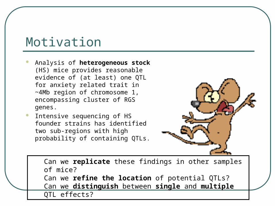
Motivation Analysis of heterogeneous stock

(HS) mice provides reasonable evidence of (at least) one QTL for anxiety related trait in ~4Mb region of chromosome 1, encompassing cluster of RGS genes.

Intensive sequencing of HS founder strains has identified two sub-regions with high probability of containing QTLs.

Can we replicate these findings in other samples of mice?Can we refine the location of potential QTLs?Can we distinguish between single and multiple QTL effects?

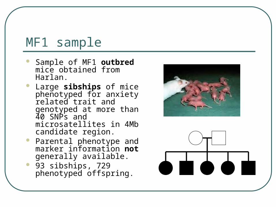
MF1 sample Sample of MF1 outbred mice

obtained from Harlan. Large sibships of mice

phenotyped for anxiety related trait and genotyped at more than 40 SNPs and microsatellites in 4Mb candidate region.

Parental phenotype and marker information not generally available.

93 sibships, 729 phenotyped offspring.

Method outline Reconstruct marker haplotypes in sibships

and estimate inheritance vectors, taking account of uncertainty in phase assignment.

Approximate distribution of location of di-allelic QTL(s) (mutant/normal) in candidate region given phenotypes and inheritance vectors, allowing for uncertainty in parental QTL alleles.

Compare additive vs dominant genetic effect models and single QTL vs multiple QTL models.

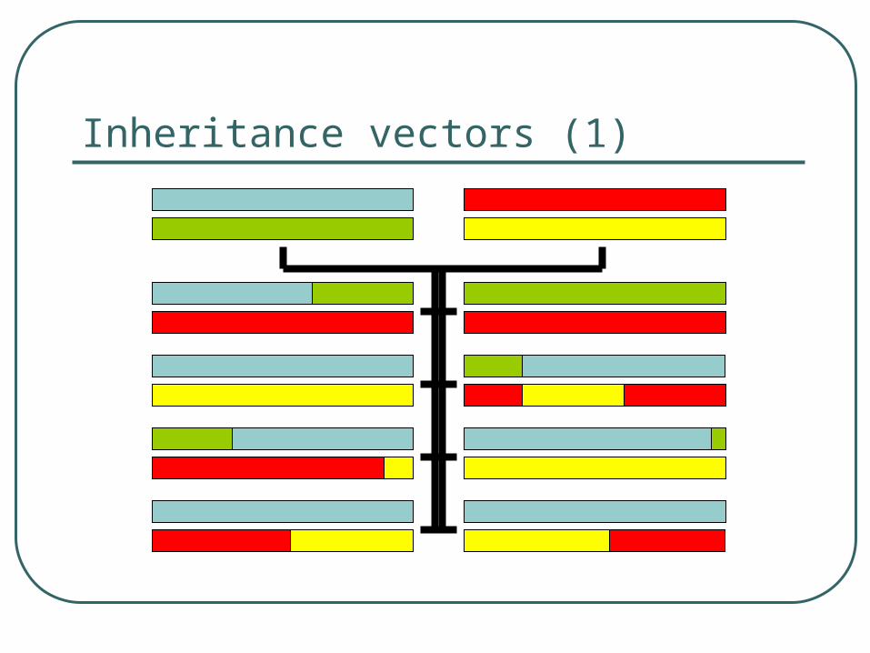
Inheritance vectors (1)

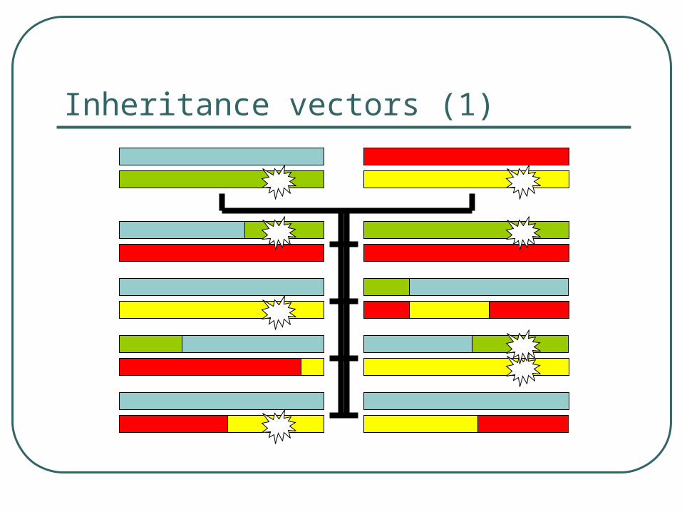
Inheritance vectors (1)

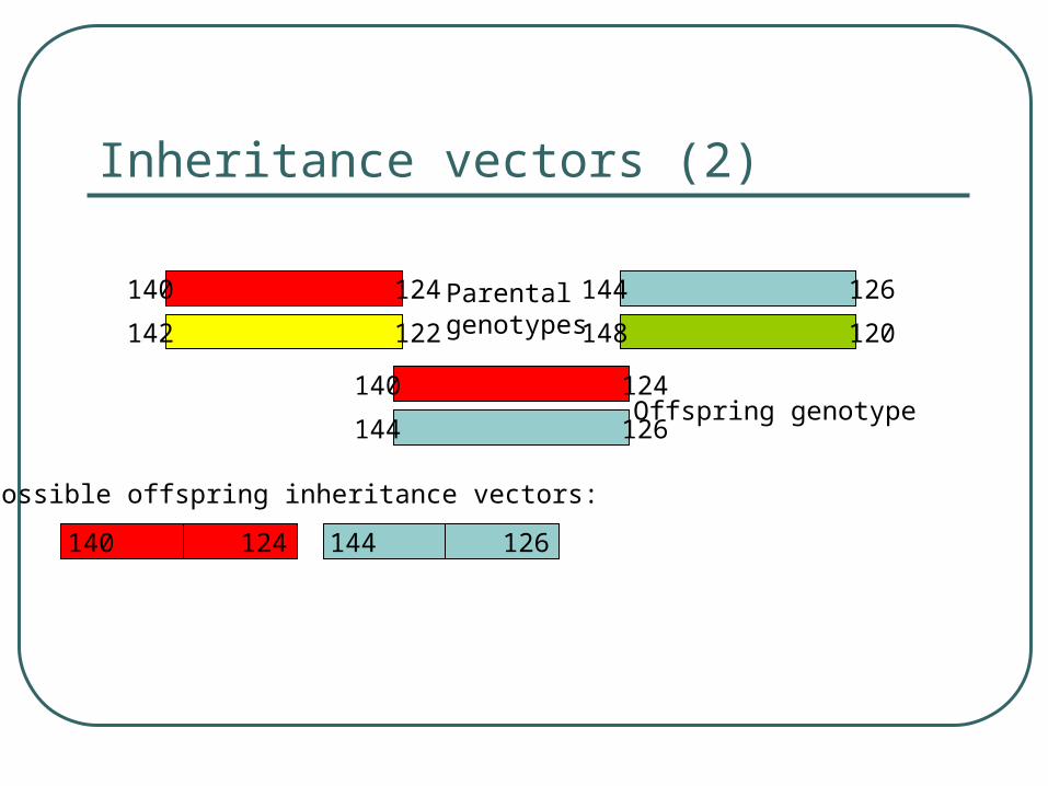
Inheritance vectors (2)

140 124

142 122

Parental genotypes

Possible offspring inheritance vectors:

140 124

148 120

144 126

140 124

144 126Offspring genotype

144 126

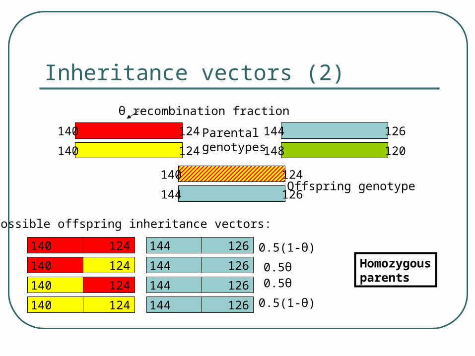
Inheritance vectors (2)

140 124

140 124

θ recombination fraction

Parental genotypes

Possible offspring inheritance vectors:

140 124

140

140

140

124

124

124

0.5(1-θ)

0.5θ0.5θ

0.5(1-θ)

Homozygousparents

148 120

144 126

140 124

144 126Offspring genotype

144 126

144

144

144

126

126

126

Inheritance vectors (2)

140

142

θ recombination fraction

Parental genotypes

Possible offspring inheritance vectors:

140 124

140 124

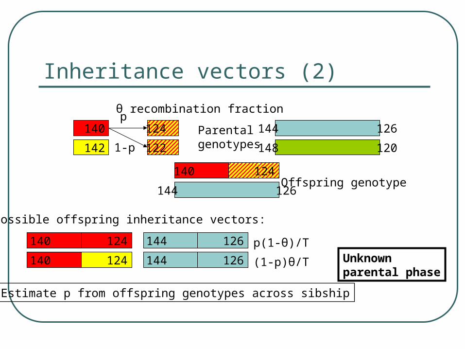
p(1-θ)/T

(1-p)θ/T Unknownparental phase

148 120

144 126

140

144 126Offspring genotype

144 126

144 126

124

122

124 p

1-p

Estimate p from offspring genotypes across sibship

Inheritance vectors (2)

θ recombination fraction

Parental genotypes

Possible offspring inheritance vectors:

140 124

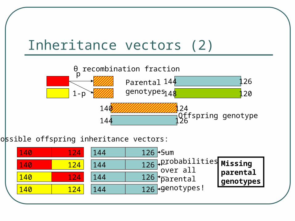
140 124 Missingparentalgenotypes

148 120

144 126

144 126Offspring genotype

144 126

144 126

140 124

p

1-p

140

140

124

124

144

144

126

126

Sumprobabilitiesover allparentalgenotypes!

Inheritance vectors (2)

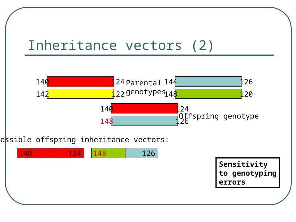
140 124

142 122

Parental genotypes

Possible offspring inheritance vectors:

140 124

148 120

144 126

140 124

148 126Offspring genotype

148 126

Sensitivityto genotypingerrors

Inhertitance vectors (3)

For MF1 sample, parental genotypes not currently available.

Too many combinations of parental genotypes to consider all markers simultaneously.

Use overlapping sliding window of five markers, and combine information across windows.

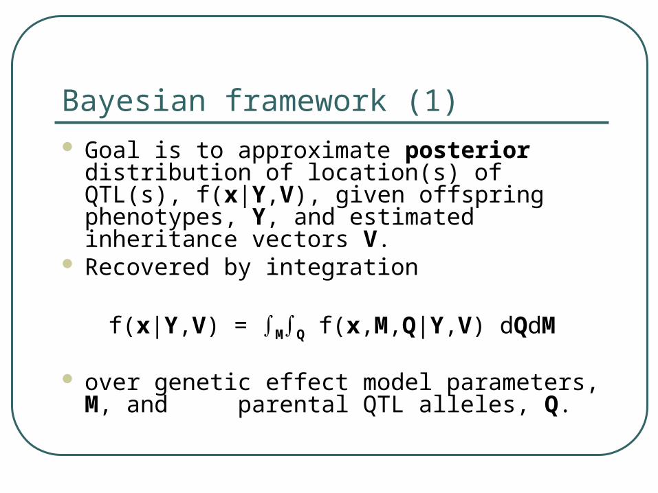
Bayesian framework (1) Goal is to approximate posterior distribution of

location(s) of QTL(s), f(x|Y,V), given offspring phenotypes, Y, and estimated inheritance vectors V.

Recovered by integration

f(x|Y,V) = ∫M∫Q f(x,M,Q|Y,V) dQdM

over genetic effect model parameters, M, and parental QTL alleles, Q.

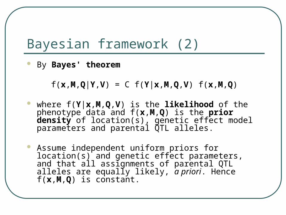
Bayesian framework (2) By Bayes' theorem

f(x,M,Q|Y,V) = C f(Y|x,M,Q,V) f(x,M,Q)

where f(Y|x,M,Q,V) is the likelihood of the phenotype data and f(x,M,Q) is the prior density of location(s), genetic effect model parameters and parental QTL alleles.

Assume independent uniform priors for location(s) and genetic effect parameters, and that all assignments of parental QTL alleles are equally likely, a priori. Hence f(x,M,Q) is constant.

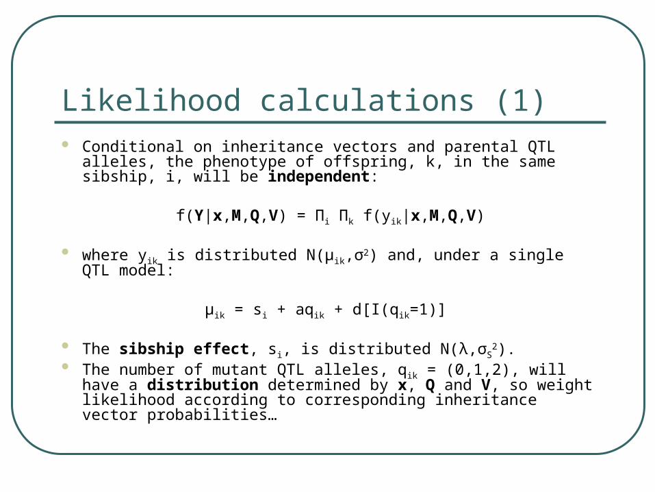
Likelihood calculations (1) Conditional on inheritance vectors and parental QTL alleles, the

phenotype of offspring, k, in the same sibship, i, will be independent:

f(Y|x,M,Q,V) = Πi Πk f(yik|x,M,Q,V)

where yik is distributed N(μik,σ2) and, under a single QTL model:

μik = si + aqik + d[I(qik=1)]

The sibship effect, si, is distributed N(λ,σS2).

The number of mutant QTL alleles, qik = (0,1,2), will have a distribution determined by x, Q and V, so weight likelihood according to corresponding inheritance vector probabilities…

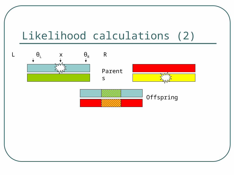
Likelihood calculations (2)

L θL x θR R

Parents

Offspring

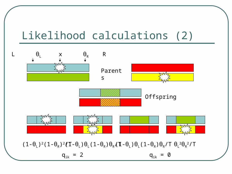
Likelihood calculations (2)

L θL x θR R

Parents

Offspring

(1-θL)2(1-θR)2/T (1-θL)θL(1-θR)θR/T θL2θR

2/T(1-θL)θL(1-θR)θR/T

qik = 1 qik = 2 qik = 0 qik = 1

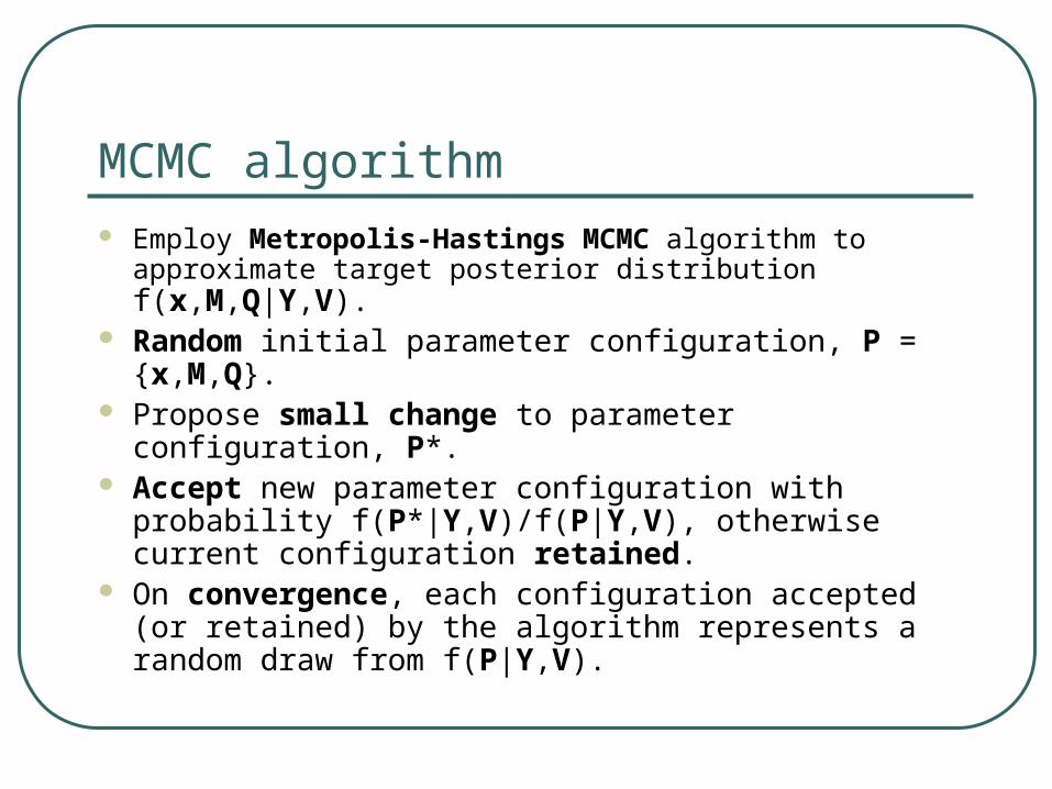
MCMC algorithm Employ Metropolis-Hastings MCMC algorithm to

approximate target posterior distribution f(x,M,Q|Y,V). Random initial parameter configuration, P = {x,M,Q}. Propose small change to parameter configuration,

P*. Accept new parameter configuration with probability

f(P*|Y,V)/f(P|Y,V), otherwise current configuration retained.

On convergence, each configuration accepted (or retained) by the algorithm represents a random draw from f(P|Y,V).

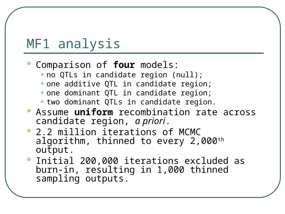
MF1 analysis Comparison of four models:

• no QTLs in candidate region (null);• one additive QTL in candidate region;• one dominant QTL in candidate region;• two dominant QTLs in candidate region.

Assume uniform recombination rate across candidate region, a priori.

2.2 million iterations of MCMC algorithm, thinned to every 2,000th output.

Initial 200,000 iterations excluded as burn-in, resulting in 1,000 thinned sampling outputs.

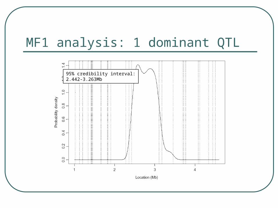
MF1 analysis: 1 dominant QTL

95% credibility interval:2.442-3.263Mb

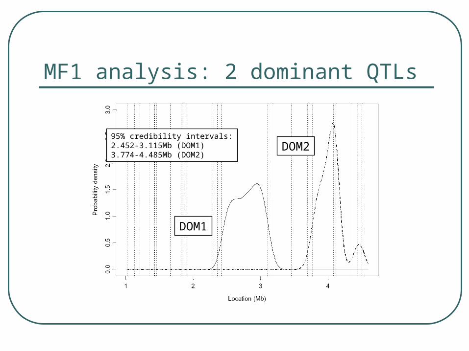
MF1 analysis: 2 dominant QTLs

95% credibility intervals:2.452-3.115Mb (DOM1)3.774-4.485Mb (DOM2)

DOM1

DOM2

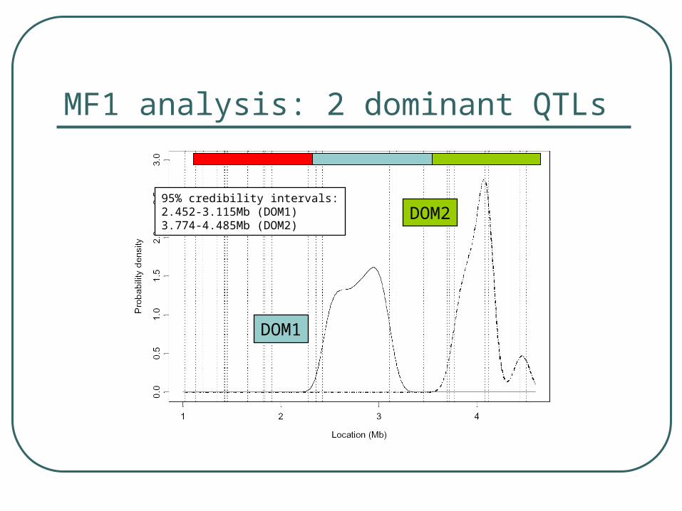
MF1 analysis: 2 dominant QTLs

95% credibility intervals:2.452-3.115Mb (DOM1)3.774-4.485Mb (DOM2)

DOM1

DOM2

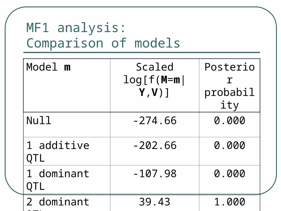
MF1 analysis:Comparison of models

Model m Scaled log[f(M=m|Y,V)]

Posterior probability

Null -274.66 0.000

1 additive QTL -202.66 0.000

1 dominant QTL -107.98 0.000

2 dominant QTLs 39.43 1.000

MF1 analysis: ongoing work

Model 3 dominant QTLs in candidate region. Incorporate parental genotype information. Additional genotyping in vicinity of DOM1. Sensitivity to marker selection and

genotyping error. Investigate properties of algorithm under null

model by random permutation of offspring phenotypes.

Summary

Bayesian MCMC method developed to approximate distribution of location of QTLs in candidate region.

Designed for use with large sibships of outbred mice, but could be generalised to other pedigree structures.

Analysis of MF1 sample suggests evidence of (at least) two QTLs, one in the vicinity of RGS18.