Bayesian Inference

Statisticat, LLC

Abstract

The Bayesian interpretation of probability is one of two broad categories of interpre-tations. Bayesian inference updates knowledge about unknowns, parameters, with infor-mation from data. The LaplacesDemon package is a complete environment for Bayesianinference within R, and this vignette provides an introduction to the topic. This arti-cle introduces Bayes’ theorem, model-based Bayesian inference, components of Bayesianinference, prior distributions, hierarchical Bayes, conjugacy, likelihood, numerical approx-imation, prediction, Bayes factors, model fit, posterior predictive checks, and ends bycomparing advantages and disadvantages of Bayesian inference.

Keywords:˜Bayesian, Laplace’s Demon, LaplacesDemon, R, Statisticat.

This article is an introduction to Bayesian inference for users of the LaplacesDemon package(Statisticat LLC. 2013) in R (R Development Core Team 2012), otherwise referred to asLaplace’s Demon. A formal introduction to Laplace’s Demon is provided in an accompanyingvignette entitled “LaplacesDemon Tutorial”. Merriam-Webster defines ‘Bayesian’ as follows

Bayesian : being, relating to, or involving statistical methods that assign proba-bilities or distributions to events (as rain tomorrow) or parameters (as a populationmean) based on experience or best guesses before experimentation and data col-lection and that apply Bayes’ theorem to revise the probabilities and distributionsafter obtaining experimental data.

In statistical inference, there are two broad categories of interpretations of probability: Bayesianinference and frequentist inference. These views often differ with each other on the fundamen-tal nature of probability. Frequentist inference loosely defines probability as the limit of anevent’s relative frequency in a large number of trials, and only in the context of experimentsthat are random and well-defined. Bayesian inference, on the other hand, is able to assignprobabilities to any statement, even when a random process is not involved. In Bayesianinference, probability is a way to represent an individual’s degree of belief in a statement, orgiven evidence.

Within Bayesian inference, there are also different interpretations of probability, and differentapproaches based on those interpretations. The most popular interpretations and approaches

2 Bayesian Inference

are objective Bayesian inference (Berger 2006) and subjective Bayesian inference (Anscombeand Aumann 1963; Goldstein 2006). Objective Bayesian inference is often associated withBayes and Price (1763), Laplace (1814), and Jeffreys (1961). Subjective Bayesian inference isoften associated with Ramsey (1926), De˜Finetti (1931), and Savage (1954). The first majorevent to bring about the rebirth of Bayesian inference was De˜Finetti (1937). Differences inthe interpretation of probability are best explored outside of this article1.

This article is intended as an approachable introduction to Bayesian inference, or as a handysummary for experienced Bayesians. It is assumed that the reader has at least an elemen-tary understanding of statistics, and this article focuses on applied, rather than theoretical,material. Equations and statistical notation are included, but it is hopefully presented so thereader does not need an intricate understanding of solving integrals, for example, but shouldunderstand the basic concept of integration. Please be aware that it is difficult to summarizeBayesian inference in such a short article. In which case, consider Gelman, Carlin, Stern, andRubin (2004) for a more thorough and formal introduction.

1. Bayes’ Theorem

Bayes’ theorem shows the relation between two conditional probabilities that are the reverseof each other. This theorem is named after Reverend Thomas Bayes (1701-1761), and is alsoreferred to as Bayes’ law or Bayes’ rule (Bayes and Price 1763)2. Bayes’ theorem expressesthe conditional probability, or ‘posterior probability’, of an event A after B is observed interms of the ‘prior probability’ of A, prior probability of B, and the conditional probabilityof B given A. Bayes’ theorem is valid in all common interpretations of probability. The two(related) examples below should be sufficient to introduce Bayes’ theorem.

1.1. Bayes’ Theorem, Example 1

Bayes’ theorem provides an expression for the conditional probability of A given B, which isequal to

Pr(A|B) =Pr(B|A) Pr(A)

Pr(B)(1)

For example, suppose one asks the question: what is the probability of going to Hell, condi-tional on consorting (or given that a person consorts) with Laplace’s Demon3. By replacingA with Hell and B with Consort, the question becomes

Pr(Hell|Consort) =Pr(Consort|Hell) Pr(Hell)

Pr(Consort)

1If these terms are new to the reader, then please do not focus too much on the words ‘objective’ and‘subjective’, since there is a lot of debate over them. For what it’s worth, Statisticat, LLC, the provider of thisR package entitled LaplacesDemon, favors the ‘subjective’ interpretation.

2Stigler (1983) suggests the earliest discoverer of Bayes’ theorem was Nicholas Saunderson (1682-1739), ablind mathematician/optician, who at age 29 became the Lucasian Professor of Mathematics at Cambridge.This position was previously held by Isaac Newton.

3This example is, of course, intended with humor.

Statisticat LLC 3

Note that a common fallacy is to assume that Pr(A|B) = Pr(B|A), which is called theconditional probability fallacy.

1.2. Bayes’ Theorem, Example 2

Another way to state Bayes’ theorem is

Pr(Ai|B) =Pr(B|Ai) Pr(Ai)

Pr(B|Ai) Pr(Ai) + ...+ Pr(B|An) Pr(An)

Let’s examine our burning question, by replacing Ai with Hell or Heaven, and replacing Bwith Consort

• Pr(A1) = Pr(Hell)

• Pr(A2) = Pr(Heaven)

• Pr(B) = Pr(Consort)

• Pr(A1|B) = Pr(Hell|Consort)

• Pr(A2|B) = Pr(Heaven|Consort)

• Pr(B|A1) = Pr(Consort|Hell)

• Pr(B|A2) = Pr(Consort|Heaven)

Laplace’s Demon was conjured and asked for some data. He was glad to oblige.

Data

• 6 people consorted out of 9 who went to Hell.

• 5 people consorted out of 7 who went to Heaven.

• 75% of the population goes to Hell.

• 25% of the population goes to Heaven.

Now, Bayes’ theorem is applied to the data. Four pieces are worked out as follows

• Pr(Consort|Hell) = 6/9 = 0.666

• Pr(Consort|Heaven) = 5/7 = 0.714

• Pr(Hell) = 0.75

• Pr(Heaven) = 0.25

Finally, the desired conditional probability Pr(Hell|Consort) is calculated using Bayes’ theo-rem

• Pr(Hell|Consort) = 0.666(0.75)0.666(0.75)+0.714(0.25)

4 Bayesian Inference

• Pr(Hell|Consort) = 0.737

The probability of someone consorting with Laplace’s Demon and going to Hell is 73.7%,which is less than the prevalence of 75% in the population. According to these findings,consorting with Laplace’s Demon does not increase the probability of going to Hell. Withthat in mind, please continue. . .

2. Model-Based Bayesian Inference

The basis for Bayesian inference is derived from Bayes’ theorem. Here is Bayes’ theorem,equation 1, again

Pr(A|B) =Pr(B|A) Pr(A)

Pr(B)

Replacing B with observations y, A with parameter set Θ, and probabilities Pr with densitiesp (or sometimes π or function f), results in the following

p(Θ|y) =p(y|Θ)p(Θ)

p(y)

where p(y) will be discussed below, p(Θ) is the set of prior distributions of parameter setΘ before y is observed, p(y|Θ) is the likelihood of y under a model, and p(Θ|y) is the jointposterior distribution, sometimes called the full posterior distribution, of parameter set Θthat expresses uncertainty about parameter set Θ after taking both the prior and data intoaccount. Since there are usually multiple parameters, Θ represents a set of j parameters, andmay be considered hereafter in this article as

Θ = θ1, ..., θj

The denominator

p(y) =

∫p(y|Θ)p(Θ)dΘ

defines the “marginal likelihood” of y, or the “prior predictive distribution” of y, and may beset to an unknown constant c. The prior predictive distribution4 indicates what y shouldlook like, given the model, before y has been observed. Only the set of prior probabilities andthe model’s likelihood function are used for the marginal likelihood of y. The presence of themarginal likelihood of y normalizes the joint posterior distribution, p(Θ|y), ensuring it is aproper distribution and integrates to one.

By replacing p(y) with c, which is short for a ‘constant of proportionality’, the model-basedformulation of Bayes’ theorem becomes

p(Θ|y) =p(y|Θ)p(Θ)

c

4The predictive distribution was introduced by Jeffreys (1961).

Statisticat LLC 5

By removing c from the equation, the relationship changes from ’equals’ (=) to ’proportionalto’ (∝)5

p(Θ|y) ∝ p(y|Θ)p(Θ) (2)

This form can be stated as the unnormalized joint posterior being proportional to the like-lihood times the prior. However, the goal in model-based Bayesian inference is usually notto summarize the unnormalized joint posterior distribution, but to summarize the marginaldistributions of the parameters. The full parameter set Θ can typically be partitioned into

Θ = {Φ,Λ}

where Φ is the sub-vector of interest, and Λ is the complementary sub-vector of Θ, oftenreferred to as a vector of nuisance parameters. In a Bayesian framework, the presence ofnuisance parameters does not pose any formal, theoretical problems. A nuisance parameteris a parameter that exists in the joint posterior distribution of a model, though it is not aparameter of interest. The marginal posterior distribution of φ, the parameter of interest,can simply be written as

p(φ|y) =

∫p(φ,Λ|y)dΛ

In model-based Bayesian inference, Bayes’ theorem is used to estimate the unnormalized jointposterior distribution, and finally the user can assess and make inferences from the marginalposterior distributions.

3. Components of Bayesian Inference

The components6 of Bayesian inference are

1. p(Θ) is the set of prior distributions for parameter set Θ, and uses probability as ameans of quantifying uncertainty about Θ before taking the data into account.

2. p(y|Θ) is the likelihood or likelihood function, in which all variables are related in a fullprobability model.

3. p(Θ|y) is the joint posterior distribution that expresses uncertainty about parameterset Θ after taking both the prior and the data into account. If parameter set Θ ispartitioned into a single parameter of interest φ and the remaining parameters areconsidered nuisance parameters, then p(φ|y) is the marginal posterior distribution.

4. Prior Distributions

5For those unfamiliar with ∝, this symbol simply means that two quantities are proportional if they varyin such a way that one is a constant multiplier of the other. This is due to the constant of proportionality cin the equation. Here, this can be treated as ‘equal to’.

6In Bayesian decision theory, an additional component exists (Roberts 2007, p. 53), the loss function,L(Θ,∆).

6 Bayesian Inference

In Bayesian inference, a prior probability distribution, often called simply the prior, of anuncertain parameter θ or latent variable is a probability distribution that expresses uncertaintyabout θ before the data are taken into account7. The parameters of a prior distribution arecalled hyperparameters, to distinguish them from the parameters (Θ) of the model.

When applying Bayes’ theorem, the prior is multiplied by the likelihood function and thennormalized to estimate the posterior probability distribution, which is the conditional distri-bution of Θ given the data. Moreover, the prior distribution affects the posterior distribution.

Prior probability distributions have traditionally belonged to one of two categories: informa-tive priors and uninformative priors. Here, four categories of priors are presented accordingto information8 and the goal in the use of the prior. The four categories are informative,weakly informative, least informative, and uninformative.

4.1. Informative Priors

When prior information is available about θ, it should be included in the prior distribution ofθ. For example, if the present model form is similar to a previous model form, and the presentmodel is intended to be an updated version based on more current data, then the posteriordistribution of θ from the previous model may be used as the prior distribution of θ for thepresent model.

In this way, each version of a model is not starting from scratch, based only on the presentdata, but the cumulative effects of all data, past and present, can be taken into account. Toensure the current data do not overwhelm the prior, Ibrahim and Chen (2000) introduced thepower prior. The power prior is a class of informative prior distribution that takes previousdata and results into account. If the present data is very similar to the previous data, then theprecision of the posterior distribution increases when including more and more informationfrom previous models. If the present data differs considerably, then the posterior distributionof θ may be in the tails of the prior distribution for θ, so the prior distribution contributesless density in its tails.

Sometimes informative prior information is not simply ready to be used, such as when it residesin another person, as in an expert. In this case, their personal beliefs about the probability ofthe event must be elicited into the form of a proper probability density function. This processis called prior elicitation.

4.2. Weakly Informative Priors

Weakly Informative Prior (WIP) distributions use prior information for regularization9 andstabilization, providing enough prior information to prevent results that contradict our knowl-

7One so-called version of Bayesian inference is ‘empirical Bayes’, which sounds enticing because anything‘empirical’ seems desirable. However, empirical Bayes is a term for the use of data-dependent priors, wherethe prior is first modeled usually with maximum likelihood and then used in the Bayesian model. This is anundesirable double-use of the data and is most problematic with small sample sizes (Berger 2006). It alsoseems to violate the elementary concept that a prior probability distribution expresses uncertainty about θbefore the data are taken into account. It has been claimed that “empirical Bayes methods are not Bayesian”(Bernardo 2008).

8‘Information’ is used loosely here to describe either the prior information from personal beliefs orinformational-theoretic content.

9The definition of regularization is to introduce additional information in order to solve an ill-posed problemor to prevent overfitting.

Statisticat LLC 7

edge or problems such as an algorithmic failure to explore the state-space. Another goal is forWIPs to use less prior information than is actually available. A WIP should provide some ofthe benefit of prior information while avoiding some of the risk from using information thatdoesn’t exist. WIPs are the most common priors in practice, and are favored by subjectiveBayesians.

Selecting a WIP can be tricky. WIP distributions should change with the sample size, becausea model should have enough prior information to learn from the data, but the prior informationmust also be weak enough to learn from the data.

Following is an example of a WIP in practice. It is popular, for good reasons, to center andscale all continuous predictors (Gelman 2008). Although centering and scaling predictors isnot discussed here, it should be obvious that the potential range of the posterior distributionof θ for a centered and scaled predictor should be small. A popular WIP for a centered andscaled predictor may be

θ ∼ N (0, 10000)

where θ is normally-distributed according to a mean of 0 and a variance of 10,000, which isequivalent to a standard deviation of 100, or precision of 1.0E-4. In this case, the density forθ is nearly flat. Nonetheless, the fact that it is not perfectly flat yields good properties fornumerical approximation algorithms. In both Bayesian and frequentist inference, it is possiblefor numerical approximation algorithms to become stuck in regions of flat density, whichbecome more common as sample size decreases or model complexity increases. Numericalapproximation algorithms in frequentist inference function as though a flat prior were used,so numerical approximation algorithms in frequentist inference become stuck more frequentlythan numerical approximation algorithms in Bayesian inference. Prior distributions that arenot completely flat provide enough information for the numerical approximation algorithm tocontinue to explore the target density, the posterior distribution.

After updating a model in which WIPs exist, the user should examine the posterior to see if theposterior contradicts knowledge. If the posterior contradicts knowledge, then the WIP mustbe revised by including information that will make the posterior consistent with knowledge(Gelman 2008).

A popular objective Bayeisan criticism against WIPs is that there is no precise, mathematicalform to derive the optimal WIP for a given model and data.

Vague Priors

A vague prior, also called a diffuse prior10, is difficult to define, after considering WIPs.The first formal move from vague to weakly informative priors is Lambert, Sutton, Burton,Abrams, and Jones (2005). After conjugate priors were introduced (Raiffa and Schlaifer1961), most applied Bayesian modeling has used vague priors, parameterized to approximatethe concept of uninformative priors (better considered as least informative priors, see section4.3). For more information on conjugate priors, see section 6.

Typically, a vague prior is a conjugate prior with a large scale parameter. However, vaguepriors can pose problems when the sample size is small. Most problems with vague priors andsmall sample size are associated with scale, rather than location, parameters. The problem

10Some sources refer to diffuse priors as flat priors.

8 Bayesian Inference

can be particularly acute in random-effects models, and the term random-effects is used ratherloosely here to imply exchangeable11, hierarchical, and multilevel structures. A vague prioris defined here as usually being a conjugate prior that is intended to approximate an uninfor-mative prior (or actually, a least informative prior), and without the goals of regularizationand stabilization.

4.3. Least Informative Priors

The term ‘Least Informative Priors’, or LIPs, is used here to describe a class of prior in whichthe goal is to minimize the amount of subjective information content, and to use a prior thatis determined solely by the model and observed data. The rationale for using LIPs is oftensaid to be ‘to let the data speak for themselves’. LIPs are favored by objective Bayesians.

Flat Priors

The flat prior was historically the first attempt at an uninformative prior. The unbounded,uniform distribution, often called a flat prior, is

θ ∼ U(−∞,∞)

where θ is uniformly-distributed from negative infinity to positive infinity. Although thisseems to allow the posterior distribution to be affected soley by the data with no impactfrom prior information, this should generally be avoided because this probability distributionis improper, meaning it will not integrate to one since the integral of the assumed p(θ) isinfinity (which violates the assumption that the probabilities sum to one). This may causethe posterior to be improper, which invalidates the model.

Reverend Thomas Bayes (1701-1761) was the first to use inverse probability (Bayes and Price1763), and used a flat prior for his billiard example so that all possible values of θ are equallylikely a priori (Gelman et˜al. 2004, p. 34-36). Pierre-Simon Laplace (1749-1827) also used theflat prior to estimate the proportion of female births in a population, and for all estimationproblems presented or justified as a reasonable expression of ignorance. Laplace’s use ofthis prior distribution was later referred to as the ‘principle of indifference’ or ‘principle ofinsufficient reason’, and is now called the flat prior (Gelman et˜al. 2004, p. 39). Laplace wasaware that it was not truly uninformative, and used it as a LIP.

Another problem with the flat prior is that it is not invariant to transformation. For example,a flat prior on a standard deviation parameter is not also flat for its variance or precision.

Hierarchical Prior

A hierarchical prior is a prior in which the parameters of the prior distribution are estimatedfrom data via hyperpriors, rather than with subjective information (Gelman 2008). Parame-ters of hyperprior distributions are called hyperparameters. Subjective Bayesians prefer thehierarchical prior as the LIP, and the hyperparameters are usually specified as WIPs. Hier-archical priors are presented later in more detail in the section entitled ‘Hierarchical Bayes’.

Jeffreys Prior

11For more information on exchangeability, see http://www.bayesian-inference.com/exchangeability.

Statisticat LLC 9

Jeffreys prior, also called Jeffreys rule, was introduced in an attempt to establish a leastinformative prior that is invariant to transformations (Jeffreys 1961). Jeffreys prior workswell for a single parameter, but multi-parameter situations may have inappropriate aspectsaccumulate across dimensions to detrimental effect.

MAXENT

A MAXENT prior, proposed by Jaynes (1968), is a prior probability distribution that isselected among other candidate distributions as the prior of choice when it has the maximumentropy (MAXENT) in the considered set, given constraints on the candidate set. Moreentropy is associated with less information, and the least informative prior is preferred as aMAXENT prior. The principle of minimum cross-entropy generalizes MAXENT priors frommere selection to updating the prior given constraints while seeking the maximum, possibleentropy.

Reference Priors

Introduced by Bernardo (1979), reference priors do not express personal beliefs. Instead,reference priors allow the data to dominate the prior and posterior (Berger, Bernardo, andDongchu 2009). Reference priors are estimated by maximizing the expected intrinsic discrep-ancy between the posterior distribution and prior distribution. This maximizes the expectedposterior information about y when the prior density is p(y). In some sense, p(y) is the ‘leastinformative’ prior about y (Bernardo 2005). Reference priors are often the objective priorof choice in multivariate problems, since other rules (e.g., Jeffreys rule) may result in priorswith problematic behavior. When reference priors are used, the analysis is called referenceanalysis, and the posterior is called the reference posterior.

Subjective Bayesian criticisms of reference priors are that the concepts of regularization andstabilization are not taken into account, results that contradict knowledge are not prevented,a numerical approximation algorithm may become stuck in low-probability or flat regions,and it may not be desirable to let the data speak fully.

4.4. Uninformative Priors

Traditionally, most of the above descriptions of prior distributions were categorized as unin-formative priors. However, uninformative priors do not truly exist (Irony and Singpurwalla1997), and all priors are informative in some way. Traditionally, there have been many namesassociated with uninformative priors, including diffuse, minimal, non-informative, objective,reference, uniform, vague, and perhaps weakly informative.

4.5. Proper and Improper Priors

It is important for the prior distribution to be proper. A prior distribution, p(θ), is improper12

when ∫p(θ)dθ =∞

12Improper priors were introduced in Jeffreys (1961).

10 Bayesian Inference

As noted previously, an unbounded uniform prior distribution is an improper prior distributionbecause p(θ) ∝ 1, for −∞ < θ < ∞. An improper prior distribution can cause an improperposterior distribution. When the posterior distribution is improper, inferences are invalid, itis non-integrable, and Bayes factors cannot be used (though there are exceptions).

To determine the propriety of a joint posterior distribution, the marginal likelihood must befinite for all y. Again, the marginal likelihood is

p(y) =

∫p(y|Θ)p(Θ)dΘ

Although improper prior distributions can be used, it is good practice to avoid them.

5. Hierarchical Bayes

Prior distributions may be estimated within the model via hyperprior distributions, which areusually vague and nearly flat. Parameters of hyperprior distributions are called hyperparam-eters. Using hyperprior distributions to estimate prior distributions is known as hierarchicalBayes. In theory, this process could continue further, using hyper-hyperprior distributionsto estimate the hyperprior distributions. Estimating priors through hyperpriors, and fromthe data, is a method to elicit the optimal prior distributions. One of many natural uses forhierarchical Bayes is multilevel modeling.

Recall that the unnormalized joint posterior distribution (equation 2) is proportional to thelikelihood times the prior distribution

p(Θ|y) ∝ p(y|Θ)p(Θ)

The simplest hierarchical Bayes model takes the form

p(Θ,Φ|y) ∝ p(y|Θ)p(Θ|Φ)p(Φ)

where Φ is a set of hyperprior distributions. By reading the equation from right to left, itbegins with hyperpriors Φ, which are used conditionally to estimate priors p(Θ|Φ), whichin turn is used, as per usual, to estimate the likelihood p(y|Θ), and finally the posterior isp(Θ,Φ|y).

6. Conjugacy

When the posterior distribution p(Θ|y) is in the same family as the prior probability distri-bution p(Θ), the prior and posterior are then called conjugate distributions, and the prior iscalled a conjugate prior for the likelihood13. For example, the Gaussian family is conjugateto itself (or self-conjugate) with respect to a Gaussian likelihood function: if the likelihoodfunction is Gaussian, then choosing a Gaussian prior for the mean will ensure that the poste-rior distribution is also Gaussian. All probability distributions in the exponential family haveconjugate priors. See Gelman et˜al. (2004) for a catalog.

13The conjugate prior approach was introduced in Raiffa and Schlaifer (1961).

Statisticat LLC 11

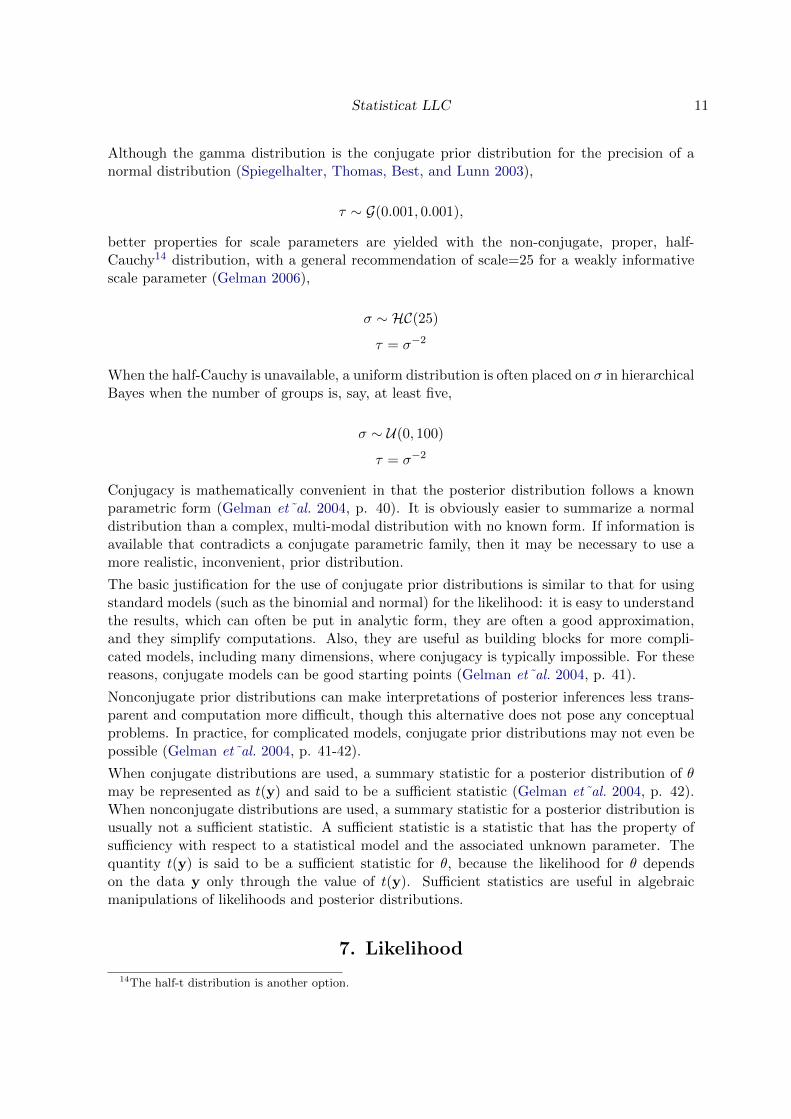
Although the gamma distribution is the conjugate prior distribution for the precision of anormal distribution (Spiegelhalter, Thomas, Best, and Lunn 2003),

τ ∼ G(0.001, 0.001),

better properties for scale parameters are yielded with the non-conjugate, proper, half-Cauchy14 distribution, with a general recommendation of scale=25 for a weakly informativescale parameter (Gelman 2006),

σ ∼ HC(25)

τ = σ−2

When the half-Cauchy is unavailable, a uniform distribution is often placed on σ in hierarchicalBayes when the number of groups is, say, at least five,

σ ∼ U(0, 100)

τ = σ−2

Conjugacy is mathematically convenient in that the posterior distribution follows a knownparametric form (Gelman et˜al. 2004, p. 40). It is obviously easier to summarize a normaldistribution than a complex, multi-modal distribution with no known form. If information isavailable that contradicts a conjugate parametric family, then it may be necessary to use amore realistic, inconvenient, prior distribution.

The basic justification for the use of conjugate prior distributions is similar to that for usingstandard models (such as the binomial and normal) for the likelihood: it is easy to understandthe results, which can often be put in analytic form, they are often a good approximation,and they simplify computations. Also, they are useful as building blocks for more compli-cated models, including many dimensions, where conjugacy is typically impossible. For thesereasons, conjugate models can be good starting points (Gelman et˜al. 2004, p. 41).

Nonconjugate prior distributions can make interpretations of posterior inferences less trans-parent and computation more difficult, though this alternative does not pose any conceptualproblems. In practice, for complicated models, conjugate prior distributions may not even bepossible (Gelman et˜al. 2004, p. 41-42).

When conjugate distributions are used, a summary statistic for a posterior distribution of θmay be represented as t(y) and said to be a sufficient statistic (Gelman et˜al. 2004, p. 42).When nonconjugate distributions are used, a summary statistic for a posterior distribution isusually not a sufficient statistic. A sufficient statistic is a statistic that has the property ofsufficiency with respect to a statistical model and the associated unknown parameter. Thequantity t(y) is said to be a sufficient statistic for θ, because the likelihood for θ dependson the data y only through the value of t(y). Sufficient statistics are useful in algebraicmanipulations of likelihoods and posterior distributions.

7. Likelihood

14The half-t distribution is another option.

12 Bayesian Inference

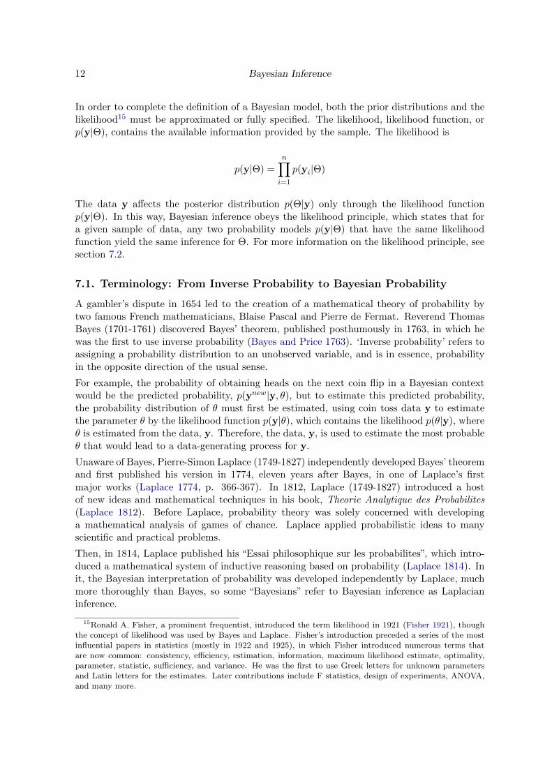
In order to complete the definition of a Bayesian model, both the prior distributions and thelikelihood15 must be approximated or fully specified. The likelihood, likelihood function, orp(y|Θ), contains the available information provided by the sample. The likelihood is

p(y|Θ) =

n∏i=1

p(yi|Θ)

The data y affects the posterior distribution p(Θ|y) only through the likelihood functionp(y|Θ). In this way, Bayesian inference obeys the likelihood principle, which states that fora given sample of data, any two probability models p(y|Θ) that have the same likelihoodfunction yield the same inference for Θ. For more information on the likelihood principle, seesection 7.2.

7.1. Terminology: From Inverse Probability to Bayesian Probability

A gambler’s dispute in 1654 led to the creation of a mathematical theory of probability bytwo famous French mathematicians, Blaise Pascal and Pierre de Fermat. Reverend ThomasBayes (1701-1761) discovered Bayes’ theorem, published posthumously in 1763, in which hewas the first to use inverse probability (Bayes and Price 1763). ‘Inverse probability’ refers toassigning a probability distribution to an unobserved variable, and is in essence, probabilityin the opposite direction of the usual sense.

For example, the probability of obtaining heads on the next coin flip in a Bayesian contextwould be the predicted probability, p(ynew|y, θ), but to estimate this predicted probability,the probability distribution of θ must first be estimated, using coin toss data y to estimatethe parameter θ by the likelihood function p(y|θ), which contains the likelihood p(θ|y), whereθ is estimated from the data, y. Therefore, the data, y, is used to estimate the most probableθ that would lead to a data-generating process for y.

Unaware of Bayes, Pierre-Simon Laplace (1749-1827) independently developed Bayes’ theoremand first published his version in 1774, eleven years after Bayes, in one of Laplace’s firstmajor works (Laplace 1774, p. 366-367). In 1812, Laplace (1749-1827) introduced a hostof new ideas and mathematical techniques in his book, Theorie Analytique des Probabilites(Laplace 1812). Before Laplace, probability theory was solely concerned with developinga mathematical analysis of games of chance. Laplace applied probabilistic ideas to manyscientific and practical problems.

Then, in 1814, Laplace published his “Essai philosophique sur les probabilites”, which intro-duced a mathematical system of inductive reasoning based on probability (Laplace 1814). Init, the Bayesian interpretation of probability was developed independently by Laplace, muchmore thoroughly than Bayes, so some “Bayesians” refer to Bayesian inference as Laplacianinference.

15Ronald A. Fisher, a prominent frequentist, introduced the term likelihood in 1921 (Fisher 1921), thoughthe concept of likelihood was used by Bayes and Laplace. Fisher’s introduction preceded a series of the mostinfluential papers in statistics (mostly in 1922 and 1925), in which Fisher introduced numerous terms thatare now common: consistency, efficiency, estimation, information, maximum likelihood estimate, optimality,parameter, statistic, sufficiency, and variance. He was the first to use Greek letters for unknown parametersand Latin letters for the estimates. Later contributions include F statistics, design of experiments, ANOVA,and many more.

Statisticat LLC 13

The term “inverse probability” appears in an 1837 paper of Augustus De Morgan (De˜Morgan1837), in reference to Laplace’s method of probability (Laplace 1774, 1812), though the term“inverse probability” does not occur in these works. Bayes’ theorem has been referred to as“the principle of inverse probability”.

Terminology has changed, so that today, Bayesian probability (rather than inverse probability)refers to assigning a probability distribution to an unobservable variable. The “distribution”of an unobserved variable given data is the likelihood function (which is not a distribution),and the distribution of an unobserved variable, given both data and a prior distribution, isthe posterior distribution. The term “Bayesian”, which displaced “inverse probability”, was infact introduced by Ronald A. Fisher as a derogatory term.

In modern terms, given a probability distribution p(y|θ) for an observable quantity y con-ditional on an unobserved variable θ, the “inverse probability” is the posterior distributionp(θ|y), which depends both on the likelihood function (the inversion of the probability distri-bution) and a prior distribution. The distribution p(y|θ) itself is called the direct probability.

However, p(y|θ) is also called the likelihood function, which can be confusing, seeming to pitthe definitions of probability and likelihood against each other. A quick introduction to thelikelihood principle follows, and finally all of the information on likelihood comes together inthe section entitled “Likelihood Function of a Parameterized Model”.

7.2. The Likelihood Principle

An informal summary of the likelihood principle may be that inferences from data to hypothe-ses should depend on how likely the actual data are under competing hypotheses, not on howlikely imaginary data would have been under a single “null” hypothesis or any other propertiesof merely possible data. Bayesian inferences depend only on the probabilities assigned due tothe observed data, not due to other data that might have been observed.

A more precise interpretation may be that inference procedures which make inferences aboutsimple hypotheses should not be justified by appealing to probabilities assigned to observationsthat have not occurred. The usual interpretation is that any two probability models with thesame likelihood function yield the same inference for θ.

Some authors mistakenly claim that frequentist inference, such as the use of maximum like-lihood estimation (MLE), obeys the likelihood, though it does not. Some authors claim thatthe largest contention between Bayesians and frequentists regards prior probability distri-butions. Other authors argue that, although the subject of priors gets more attention, thetrue contention between frequentist and Bayesian inference is the likelihood principle, whichBayesian inference obeys, and frequentist inference does not.

There have been many frequentist attacks on the likelihood principle, and have been shown tobe poor arguments. Some Bayesians have argued that Bayesian inference is incompatible withthe likelihood principle on the grounds that there is no such thing as an isolated likelihoodfunction (Bayarri and DeGroot 1987). They argue that in a Bayesian analysis there is noprincipled distinction between the likelihood function and the prior probability function. Theobjection is motivated, for Bayesians, by the fact that prior probabilities are needed in orderto apply what seems like the likelihood principle. Once it is admitted that there is a universalnecessity to use prior probabilities, there is no longer a need to separate the likelihood functionfrom the prior. Thus, the likelihood principle is accepted ‘conditional’ on the assumption thata likelihood function has been specified, but it is denied that specifying a likelihood function

14 Bayesian Inference

is necessary. Nonetheless, the likelihood principle is seen as a useful Bayesian weapon tocombat frequentism.

Following are some interesting qutoes from prominent statisticians:

“Using Bayes’ rule with a chosen probability model means that the data y affectposterior inference ’only’ through the function p(y|θ), which, when regarded as afunction of θ, for fixed y, is called the ‘likelihood function’. In this way Bayesianinference obeys what is sometimes called the ‘likelihood principle’, which statesthat for a given sample of data, any two probability models p(y|θ) that have thesame likelihood function yield the same inference for θ”(Gelman et˜al. 2004, p. 9).

“The likelihood principle is reasonable, but only within the framework of the modelor family of models adopted for a particular analysis” (Gelman et˜al. 2004, p. 9).

Frequentist “procedures typically violate the likelihood principle, since long-runbehavior under hypothetical repetitions depends on the entire distribution p(y|θ),y ∈ Y and not only on the likelihood” (Bernardo and Smith 2000, p. 454).

There is “a general fact about the mechanism of parametric Bayesian inferencewhich is trivially obvious; namely ‘for any specified p(θ), if the likelihood func-tions p1(y1|θ), p2(y2|θ) are proportional as functions of θ, the resulting posteriordensities for θ are identical’. It turns out...that many non-Bayesian inferenceprocedures do not lead to identical inferences when applied to such proportionallikelihoods. The assertion that they ‘should’, the so-called ‘Likelihood Principle’,is therefore a controversial issue among statisticians. In contrast, in the Bayesianinference context...this is a straightforward consequence of Bayes’ theorem, ratherthan an imposed ‘principle’ ” (Bernardo and Smith 2000, p. 249).

“Although the likelihood principle is implicit in Bayesian statistics, it was devel-oped as a separate principle by Barnard (Barnard 1949), and became a focus ofinterest when Birnbaum (1962) showed that it followed from the widely acceptedsufficiency and conditionality principles” (Bernardo and Smith 2000, p. 250).

“The likelihood principle, by itself, is not sufficient to build a method of inferencebut should be regarded as a minimum requirement of any viable form of inference.This is a controversial point of view for anyone familiar with modern economet-rics literature. Much of this literature is devoted to methods that do not obey thelikelihood principle...” (Rossi, Allenby, and McCulloch 2005, p. 15).

“Adherence to the likelihood principle means that inferences are ‘conditional’ onthe observed data as the likelihood function is parameterized by the data. Thisis worth contrasting to any sampling-based approach to inference. In the sam-pling literature, inference is conducted by examining the sampling distribution ofsome estimator of θ, θ̂ = f(y). Some sort of sampling experiment results in adistribution of y and therefore, the estimator is viewed as a random variable. The

Statisticat LLC 15

sampling distribution of the estimator summarizes the properties of the estimator‘prior’ to observing the data. As such, it is irrelevant to making inferences giventhe data we actually observe. For any finite sample, this dinstinction is extremelyimportant. One must conclude that, given our goal for inference, sampling distri-butions are simply not useful” (Rossi et˜al. 2005, p. 15).

7.3. Likelihood Function of a Parameterized Model

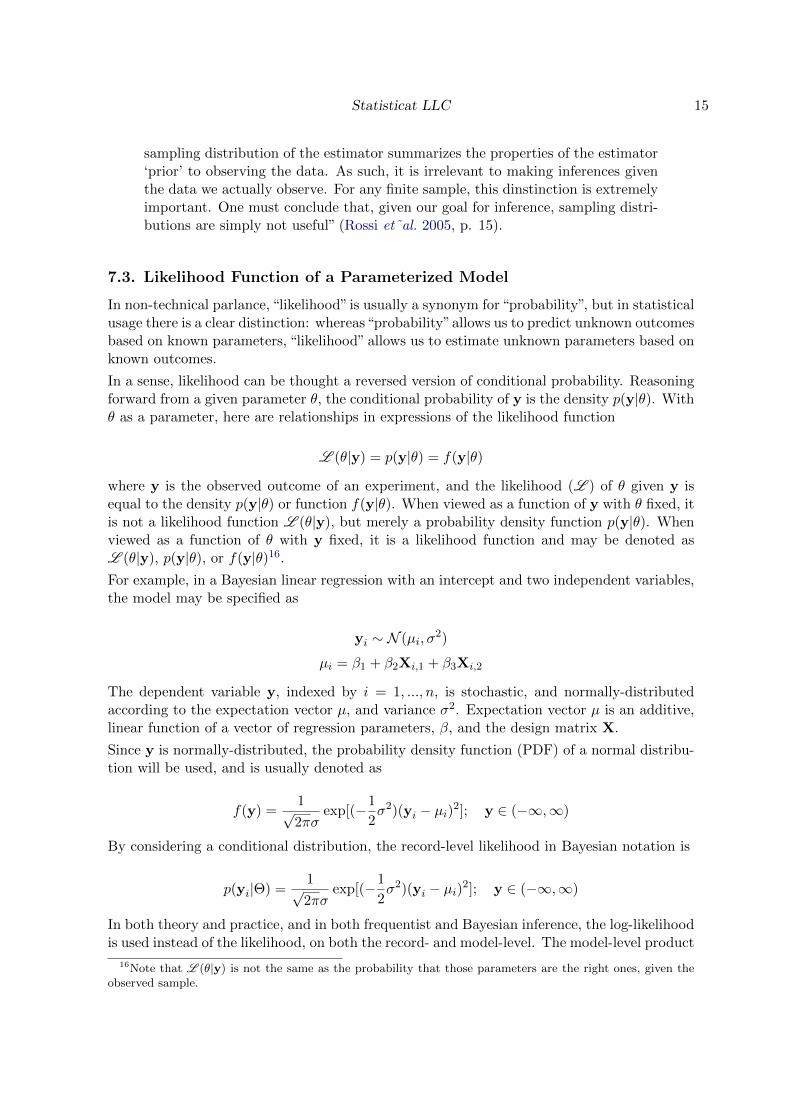
In non-technical parlance, “likelihood” is usually a synonym for“probability”, but in statisticalusage there is a clear distinction: whereas“probability”allows us to predict unknown outcomesbased on known parameters, “likelihood” allows us to estimate unknown parameters based onknown outcomes.

In a sense, likelihood can be thought a reversed version of conditional probability. Reasoningforward from a given parameter θ, the conditional probability of y is the density p(y|θ). Withθ as a parameter, here are relationships in expressions of the likelihood function

L (θ|y) = p(y|θ) = f(y|θ)

where y is the observed outcome of an experiment, and the likelihood (L ) of θ given y isequal to the density p(y|θ) or function f(y|θ). When viewed as a function of y with θ fixed, itis not a likelihood function L (θ|y), but merely a probability density function p(y|θ). Whenviewed as a function of θ with y fixed, it is a likelihood function and may be denoted asL (θ|y), p(y|θ), or f(y|θ)16.For example, in a Bayesian linear regression with an intercept and two independent variables,the model may be specified as

yi ∼ N (µi, σ2)

µi = β1 + β2Xi,1 + β3Xi,2

The dependent variable y, indexed by i = 1, ..., n, is stochastic, and normally-distributedaccording to the expectation vector µ, and variance σ2. Expectation vector µ is an additive,linear function of a vector of regression parameters, β, and the design matrix X.

Since y is normally-distributed, the probability density function (PDF) of a normal distribu-tion will be used, and is usually denoted as

f(y) =1√2πσ

exp[(−1

2σ2)(yi − µi)2]; y ∈ (−∞,∞)

By considering a conditional distribution, the record-level likelihood in Bayesian notation is

p(yi|Θ) =1√2πσ

exp[(−1

2σ2)(yi − µi)2]; y ∈ (−∞,∞)

In both theory and practice, and in both frequentist and Bayesian inference, the log-likelihoodis used instead of the likelihood, on both the record- and model-level. The model-level product

16Note that L (θ|y) is not the same as the probability that those parameters are the right ones, given theobserved sample.

16 Bayesian Inference

of record-level likelihoods can exceed the range of a number that can be stored by a computer,which is usually affected by sample size. By estimating a record-level log-likelihood, ratherthan likelihood, the model-level log-likelihood is the sum of the record-level log-likelihoods,rather than a product of the record-level likelihoods.

log[p(y|θ)] =

n∑i=1

log[p(yi|θ)]

rather than

p(y|θ) =

n∏i=1

p(yi|θ)

As a function of θ, the unnormalized joint posterior distribution is the product of the likeli-hood function and the prior distributions. To continue with the example of Bayesian linearregression, here is the unnormalized joint posterior distribution

p(β, σ2|y) = p(y|β, σ2)p(β1)p(β2)p(β3)p(σ2)

More usually, the logarithm of the unnormalized joint posterior distribution is used, which isthe sum of the log-likelihood and prior distributions. Here is the logarithm of the unnormalizedjoint posterior distribution for this example

log[p(β, σ2|y)] = log[p(y|β, σ2)] + log[p(β1)] + log[p(β2)] + log[p(β3)] + log[p(σ2)]

The logarithm of the unnormalized joint posterior distribution is maximized with numericalapproximation.

8. Numerical Approximation

The technical problem of evaluating quantities required for Bayesian inference typically re-duces to the calculation of a ratio of two integrals (Bernardo and Smith 2000, p. 339). In allcases, the technical key to the implementation of the formal solution given by Bayes’ theoremis the ability to perform a number of integrations (Bernardo and Smith 2000, p. 340). Exceptin certain rather stylized problems, the required integrations will not be feasible analyticallyand, thus, efficient approximation strategies are required.

There are too many different types of numerical approximation algorithms in Bayesian infer-ence to cover in any detail in this article. An incomplete list of broad categories of Bayesiannumerical approximation may include Approximate Bayesian Computation (ABC), Impor-tance Sampling, Iterative Quadrature, Laplace Approximation, Markov chain Monte Carlo(MCMC), and Variational Bayes (VB). Since MCMC is most common, and because the Rpackage entitled LaplacesDemon offers Importance Sampling, Laplace Approximation, andover a dozen MCMC algorithms (as well as ABC in these contexts), the following methodsare introduced below: ABC, Importance Sampling, Laplace Approximation, and MCMC. Formore information on algorithms in LaplacesDemon, see the accompanying vignette entitled“LaplacesDemon Tutorial”.

Statisticat LLC 17

Approximate Bayesian Computation (ABC), also called likelihood-free estimation, is a familyof numerical approximation techniques in Bayesian inference. ABC is especially useful whenevaluation of the likelihood, p(y|Θ) is computationally prohibitive, or when suitable likeli-hoods are unavailable. As such, ABC algorithms estimate likelihood-free approximations.ABC is usually faster than a similar likelihood-based numerical approximation technique,because the likelihood is not evaluated directly, but replaced with an approximation that isusually easier to calculate. The approximation of a likelihood is usually estimated with ameasure of distance between the observed sample, y, and its replicate given the model, yrep,or with summary statistics of the observed and replicated samples.

Importance Sampling is a method of estimating a distribution with samples from a differentdistribution, called the importance distribution. Importance weights are assigned to eachsample. The main difficulty with importance sampling is in the selection of the importancedistribution. Importance sampling is the basis of a wide variety of algorithms, some of whichinvolve the combination of importance sampling and Markov chain Monte Carlo. There arealso many variations of importance sampling, including adaptive importance sampling, andparametric and nonparametric self-normalized importance sampling. Population Monte Carlo(PMC) is based on adaptive importance sampling.

Laplace Approximation dates back to Laplace (1774, 1814), and is used to approximate theposterior moments of integrals. Specifically, the posterior mode is estimated for each param-eter, assumed to be unimodal and Gaussian. As a Gaussian distribution, the posterior meanis the same as the posterior mode, and the variance is estimated. Laplace Approximation isa family of deterministic algorithms that usually converge faster than MCMC, and just a lit-tle slower than Maximum Likelihood Estimation (MLE) (Azevedo-Filho and Shachter 1994).Laplace Approximation shares many limitations of MLE, including asymptotic estimationwith respect to sample size.

MCMC algorithms originated in statistical physics and are now used in Bayesian inference tosample from probability distributions by constructing Markov chains. In Bayesian inference,the target distribution of each Markov chain is usually a marginal posterior distribution, suchas each parameter θ. Each Markov chain begins with an initial value and the algorithm iter-ates, attempting to maximize the logarithm of the unnormalized joint posterior distributionand eventually arriving at each target distribution. Each iteration is considered a state. AMarkov chain is a random process with a finite state-space and the Markov property, meaningthat the next state depends only on the current state, not on the past. The quality of themarginal samples usually improves with the number of iterations.

A Monte Carlo method is an algorithm that relies on repeated pseudo-random sampling forcomputation, and is therefore stochastic (as opposed to deterministic). Monte Carlo methodsare often used for simulation. The union of Markov chains and Monte Carlo methods iscalled MCMC. The revival of Bayesian inference since the 1980s is due to MCMC algorithmsand increased computing power. The most prevalent MCMC algorithms may be the simplest:random-walk Metropolis and Gibbs sampling. There are a large number of MCMC algorithms,and further details on MCMC are best explored outside of this article.

9. Prediction

The “posterior predictive distribution” is either the replication of y given the model (usually

18 Bayesian Inference

represented as yrep), or the prediction of a new and unobserved y (usually represented as ynew

or y′), given the model. This is the likelihood of the replicated or predicted data, averagedover the posterior distribution p(Θ|y)

p(yrep|y) =

∫p(yrep|Θ)p(Θ|y)dΘ

or

p(ynew|y) =

∫p(ynew|Θ)p(Θ|y)dΘ

If y has missing values, then the missing ys can be estimated with the posterior predictivedistribution17 as ynew from within the model. For the linear regression example, the integralfor prediction is

p(ynew|y) =

∫p(ynew|β, σ2)p(β, σ2|y)dβdσ2

The posterior predictive distribution is easy to estimate

ynew ∼ N (µ, σ2)

where µ = Xβ, and µ is the conditional mean, while σ2 is the residual variance.

10. Bayes Factors

Introduced by Harold Jeffreys, a ‘Bayes factor’ is a Bayesian alternative to frequentist hy-pothesis testing that is most often used for the comparison of multiple models by hypothesistesting, usually to determine which model better fits the data (Jeffreys 1961). Bayes factorsare notoriously difficult to compute, and the Bayes factor is only defined when the marginaldensity of y under each model is proper. However, Bayes factors are easy to approximatewith the Laplace-Metropolis Estimator (Kass and Raftery 1995; Lewis and Raftery 1997)18.

Hypothesis testing with Bayes factors is more robust than frequentist hypothesis testing, sincethe Bayesian form avoids model selection bias, evaluates evidence in favor the null hypothesis,includes model uncertainty, and allows non-nested models to be compared (though of coursethe model must have the same dependent variable). Also, frequentist significance tests becomebiased in favor of rejecting the null hypothesis with sufficiently large sample size.

The Bayes factor for comparing two models may be approximated as the ratio of the marginallikelihood of the data in model 1 and model 2. Formally, the Bayes factor in this case is

B =p(y|M1)

p(y|M2)=

∫p(y|Θ1,M1)p(Θ1|M1)dΘ1∫p(y|Θ2,M2)p(Θ2|M2)dΘ2

17The predictive distribution was introduced by Jeffreys (1961).18A Bayes factor may be estimated with the BayesFactor function in LaplacesDemon to compare multiple

models that were fit with the LaplaceApproximation or LaplacesDemon functions. See the BayesFactor

function for the interpretation of a Bayes factor regarding strength of evidence.

Statisticat LLC 19

where p(y|M1) is the marginal likelihood of the data in model 1.

The Bayes factor, B, is the posterior odds in favor of the hypothesis divided by the prior oddsin favor of the hypothesis, where the hypothesis is usually M1 >M2. Put another way,

(Posterior model odds) = (Bayes factor) x (prior model odds)

For example, when B = 2, the data favor M1 over M2 with 2:1 odds.

In a non-hierarchical model, the marginal likelihood may easily be approximated with theLaplace-Metropolis Estimator for model m as

p(y|m) = (2π)dm/2|Σm|1/2p(y|Θm,m)p(Θm|m)

where d is the number of parameters and Σ is the inverse of the negative of the Hessian matrixof second derivatives. Lewis and Raftery (1997) introduce the Laplace-Metropolis method ofapproximating the marginal likelihood in MCMC, though it naturally works with LaplaceApproximation as well. For a hierarchical model that involves both fixed and random effects,the Compound Laplace-Metropolis Estimator must be used.

Gelman finds Bayes factors generally to be irrelevant, because they compute the relativeprobabilities of the models conditional on one of them being true. Gelman prefers approachesthat measure the distance of the data to each of the approximate models (Gelman et˜al.2004, p. 180). However, Kass and Raftery (1995) explain that “the logarithm of the marginalprobability of the data may also be viewed as a predictive score. This is of interest, becauseit leads to an interpretation of the Bayes factor that does not depend on viewing one of themodels as ‘true”’.

Two of many possible alternatives are to use

1. pseudo Bayes factors (PsBF) based on a ratio of pseudo marginal likelihoods (PsMLs)

2. Deviance Information Criterion (DIC)

DIC is the most popular method of assessing model fit and comparing models, though Bayesfactors are better, when appropriate, because they take more into account.

11. Model Fit

In Bayesian inference, the most common method of assessing the goodness of fit of an es-timated statistical model is a generalization of the frequentist Akaike Information Criterion(AIC). The Bayesian method, like AIC, is not a test of the model in the sense of hypothesistesting, though Bayesian inference has Bayes factors for such purposes. Instead, like AIC,Bayesian inference provides a model fit statistic that is to be used as a tool to refine thecurrent model or select the better-fitting model of different methodologies.

To begin with, model fit can be summarized with deviance, which is defined as -2 times thelog-likelihood (Gelman et˜al. 2004, p. 180), such as

D(y,Θ) = −2 log[p(y|Θ)]

20 Bayesian Inference

Just as with the likelihood, p(y|Θ), or log-likelihood, the deviance exists at both the record-and model-level. Due to the development of BUGS software (Gilks, Thomas, and Spiegelhalter1994), deviance is defined differently in Bayesian inference than frequentist inference. Infrequentist inference, deviance is -2 times the log-likelihood ratio of a reduced model comparedto a full model, whereas in Bayesian inference, deviance is simply -2 times the log-likelihood.In Bayesian inference, the lowest expected deviance has the highest posterior probability(Gelman et˜al. 2004, p. 181).

It is possible to have a negative deviance. Deviance is derived from the likelihood, which isderived from probability density functions (PDF). Evaluated at a certain point in parameterspace, a PDF can have a density larger than 1 due to a small standard deviation or lack ofvariation. Likelihoods greater than 1 lead to negative deviance, and are appropriate.

On its own, the deviance is an insufficient model fit statistic, because it does not take modelcomplexity into account. The effect of model fitting, pD, is used as the ‘effective number ofparameters’ of a Bayesian model. The sum of the differences between the posterior mean ofthe model-level deviance and the deviance at each draw i of θi is the pD.

A related way to measure model complexity is as half the posterior variance of the model-leveldeviance, known as pV (Gelman et˜al. 2004, p. 182)

pV = var(D)/2

The effect of model fitting, pD or pV, can be thought of as the number of ‘unconstrained’parameters in the model, where a parameter counts as: 1 if it is estimated with no constraintsor prior information; 0 if it is fully constrained or if all the information about the parametercomes from the prior distribution; or an intermediate value if both the data and the prior areinformative (Gelman et˜al. 2004, p. 182). Therefore, by including prior information, Bayesianinference is more efficient in terms of the effective number of parameters than frequentistinference. Hierarchical, mixed effects, or multilevel models are even more efficient regardingthe effective number of parameters.

Model complexity, pD or pV, should be positive. Although pV must be positive since it isrelated to variance, it is possible for pD to be negative, which indicates one or more problems:log-likelihood is non-concave, a conflict between the prior and the data, or that the posteriormean is a poor estimator (such as with a bimodal posterior).

The sum of both the mean model-level deviance and the model complexity (pD or pV) isthe Deviance Information Criterion (DIC), a model fit statistic that is also an estimate ofthe expected loss, with deviance as a loss function (Spiegelhalter, Best, and Carlin 1998;Spiegelhalter, Best, Carlin, and van˜der Linde 2002). DIC is

DIC = D̄ + pV

DIC may be compared across different models and even different methods, as long as thedependent variable does not change between models, making DIC the most flexible model fitstatistic. DIC is a hierarchical modeling generalization of the Akaike Information Criterion(AIC) and Bayesian Information Criterion (BIC). Like AIC and BIC, it is an asymptoticapproximation as the sample size becomes large. DIC is valid only when the joint posteriordistribution is approximately multivariate normal. Models should be preferred with smallerDIC. Since DIC increases with model complexity (pD or pV), simpler models are preferred.

Statisticat LLC 21

It is difficult to say what would constitute an important difference in DIC. Very roughly,differences of more than 10 might rule out the model with the higher DIC, differences between5 and 10 are substantial, but if the difference in DIC is, say, less than 5, and the models makevery different inferences, then it could be misleading just to report the model with the lowestDIC.

The Bayesian Predictive Information Criterion (BPIC) was introduced as a criterion of modelfit when the goal is to pick a model with the best out-of-sample predictive power (Ando 2007).BPIC is a variation of DIC where the effective number of parameters is 2pD (or 2pV). BPICmay be compared between ynew and yholdout, and has many other extensions, such as withBayesian Model Averaging (BMA).

12. Posterior Predictive Checks

Comparing the predictive distribution yrep to the observed data y is generally termed a“posterior predictive check”. This type of check includes the uncertainty associated with theestimated parameters of the model, unlike frequentist statistics.

Posterior predictive checks (via the predictive distribution) involve a double-use of the data,which violates the likelihood principle. However, arguments have been made in favor ofposterior predictive checks, provided that usage is limited to measures of discrepancy tostudy model adequacy, not for model comparison and inference (Meng 1994).

Gelman recommends at the most basic level to compare yrep to y, looking for any systematicdifferences, which could indicate potential failings of the model (Gelman et˜al. 2004, p. 159).It is often first recommended to compare graphical plots, such as the distribution of y andyrep. There are many posterior predictive checks that are not included in this article, but anintroduction to a selection of them appears below.

12.1. Bayesian p-values

A Bayesian form of p-value may be estimated with a variety of test statistics (Gelman, Meng,and Stern 1996). Usually the minimum or maximum observed y is compared to the minimumor maximum yrep. A Bayesian p-value is one of several ways to report discrepancies betweeny and yrep.

Frequentist p-values have many problems, but here it will only be noted that the frequen-tist p-value estimates p(data|hypothesis), while in this case the Bayesian form estimatesp(hypothesis|data). The frequentist estimates the wrong probability, because the frequen-tist is forced to consider the parameters to be fixed and the data random, projecting long-runfrequencies of what should happen with future, repeated sampling of similar data, given afixed parameter, or in this case hypothesis. Even the term hypothesis testing suggests youwant to test the hypothesis given the data, not the data given the hypothesis19.

12.2. Chi-Square

Gelman et˜al. (2004, p. 175) suggest an omnibus test such as the following χ2

19Numerous problems with frequentist p-values, confidence intervals, point estimates, and hypothesis testingare worth exploring, but not detailed in this article.

22 Bayesian Inference

χ2i =

(yi −∑T

t=1 yrepi,t

T )2

var(yrepi,1:T )

,

over records i = 1, . . . , N and posterior samples t = 1, . . . , T . The sum of χ2i over records

i = 1, . . . , N is an overall goodness of fit measure on the data set. Larger values of χ2i indicate

a worse fit for each record.

An alternative χ2 test is

p(χ2repi,1:T > χ2obs

i,1:T )

where a worse fit is indicated as p approaches zero or one, and it is common to considerrecords with a poor fit to be outside the 95% probability interval. To continue

χ2obsi,1:T =

[yi − E(yi)]2

E(yi)

and

χ2repi,1:T =

[yrepi,1:T − E(yrep

i )]2

E(yrepi )

Newer forms of χ2 tests have been proposed in the literature, and are best explored elsewhere.

12.3. Conditional Predictive Ordinate

Although the full predictive distribution p(yrep|y) is useful for prediction, its use for model-checking is questionable because of the double-use of the data, and causes predictive perfor-mance to be overestimated. The leave-one-out cross-validation predictive density has beenproposed (Geisser and Eddy 1979). This is also known as the Conditional Predictive Ordinateor CPO (Gelfand 1996).

The CPO is

p(yi|y[i]) =

∫p(yi|Θ)p(Θ|y[i])dΘ

where yi is each instance of an observed y, and y[i] is y without the current observation i.The CPO is easy to calculate with MCMC or PMC numerical approximation. By consideringthe inverse likelihood across T iterations, the CPO for each individual i is

CPOi =1

T−1T∑t=1

p(yi|Θt)−1

The CPO is a handy posterior predictive check because it may be used to identify outliers, in-fluential observations, and for hypothesis testing across different non-nested models. However,it may be difficult to calculate with latent mixtures.

Statisticat LLC 23

The CPO expresses the posterior probability of observing the value (or set of values) of yi

when the model is fitted to all data except yi, with a larger value implying a better fit of themodel to yi, and very low CPO values suggest that yi is an outlier and an influential obser-vation. A Monte Carlo estimate of the CPO is obtained without actually omitting yi fromthe estimation, and is provided by the harmonic mean of the likelihood for yi. Specifically,the CPOi is the inverse of the posterior mean of the inverse likelihood of yi.

The CPO is connected with the frequentist studentized residual test for outlier detection.Data with large studentized residuals have small CPOs and will be detected as outliers.An advantage of the CPO is that observations with high leverage will have small CPOs,independently of whether or not they are outliers. The Bayesian CPO is able to detect bothoutliers and influential points, whereas the frequentist studentized residual is unable to detecthigh-leverage outliers.

Inverse-CPOs (ICPOs) larger than 40 can be considered as possible outliers, and higher than70 as extreme values (Ntzoufras 2009, p. 376). Congdon recommends scaling CPOs by divid-ing each by its individual maximum (after the posterior mean) and considering observationswith scaled CPOs under 0.01 to be outliers (Congdon 2005). The range in scaled CPOs isuseful as an indicator of a good-fitting model.

The sum of the logged CPOs can be an estimator for the logarithm of the marginal likeli-hood20, sometimes called the log pseudo marginal likelihood (LPsML). A ratio of PsMLs isa surrogate for the Bayes factor, sometimes known as the pseudo Bayes factor (PsBF). Inthis way, non-nested models may be compared with a hypothesis test to determine the bettermodel, if one exists, based on leave-one-out cross-validation.

12.4. Predictive Concordance

Gelfand (1996) suggests that any yi that is in either 2.5% tail area of yrepi should be considered

an outlier. For each i, I am calling this the predictive quantile (PQ), which is calculated as

PQi = p(yrepi > yi)

and is somewhat similar to the Bayesian p-value. The percentage of yis that are not outliersis called the ‘Predictive Concordance’. Gelfand (1996) suggests the goal is to attempt toachieve 95% predictive concordance. In the case of, say 80% predictive concordance, thediscrepancy between the model and data is undesirable because the model does not fit thedata well and many outliers have resulted. On the other hand, if the predictive concordanceis too high, say 100%, then overfitting may have occurred, and it may be worth consideringa more parsimonious model. Kernel density plots of each yrep

i distribution are useful in thiscase with the actual yi included as a vertical bar to show its position.

12.5. L-criterion

Laud and Ibrahim (1995) introduced the L-criterion as one of three posterior predictive checksfor model, variable, and transformation selection. The L-criterion is a posterior predictivecheck that is widely applicable and easy to apply. It is a sum of two components: one involves

20Exercise extreme caution when approximating the marginal likelihood from CPOs, or use a method withbetter repute, such as the Laplace-Metropolis Estimator or importance sampling.

24 Bayesian Inference

the predictive variance and the other includes the accuracy of the means of the predictivedistribution. The L-criterion measures model performance with a combination of how closeits predictions are to the observed data and variability of the predictions. Better models havesmaller values of L. L is measured in the same units as the response variable, and measureshow close the data vector y is to the predictive distribution. In addition to the value of L,there is a value for SL, which is the calibration number of L, and is useful in determining howmuch of a decrease is necessary between models to be noteworthy. The L-criterion is

L =

N∑i=1

√var(yrep

i,1:T ) + (yi −∑T

t=1 yrepi,t

T)2,

over t = 1, . . . , T posterior samples. The calibration number, SL, is the standard deviation ofL over records i = 1, . . . , N .

Gelfand and Ghosh (1998) introduced Posterior Predictive Loss (PPL). This posterior pre-dictive check for model comparison may be viewed as an extension to the L-criterion in whicha weight k is applied to the accuracy (fit) component.

13. Advantages Of Bayesian Inference Over Frequentist Inference

Following is a short list of advantages of Bayesian inference over frequentist inference.

• Bayesian inference allows informative priors so that prior knowledge or results of aprevious model can be used to inform the current model.

• Bayesian inference can avoid problems with model identification by manipulating priordistributions (usually in complex models). Frequentist inference with any numericalapproximation algorithm does not have prior distributions, and can become stuck inregions of flat density, causing problems with model identification.

• Bayesian inference considers the data to be fixed (which it is), and parameters to berandom because they are unknowns. Frequentist inference considers the unknown pa-rameters to be fixed, and the data to be random, estimating not based on the dataat hand, but the data at hand plus hypothetical repeated sampling in the future withsimilar data. “The Bayesian approach delivers the answer to the right question in thesense that Bayesian inference provides answers conditional on the observed data andnot based on the distribution of estimators or test statistics over imaginary samples notobserved” (Rossi et˜al. 2005, p. 4).

• Bayesian inference estimates a full probability model. Frequentist inference does not.There is no frequentist probability distribution associated with parameters or hypothe-ses.

• Bayesian inference estimates p(hypothesis|data). In contrast, frequentist inference esti-mates p(data|hypothesis). Even the term ’hypothesis testing’ suggests it should be thehypothesis that is tested, given the data, not the other way around.

Statisticat LLC 25

• Bayesian inference has an axiomatic foundation (Cox 1946) that is uncontested by fre-quentists. Therefore, Bayesian inference is coherent to a frequentist, but frequentistinference is incoherent to a Bayesian.

• Bayesian inference has a decision theoretic foundation (Bernardo and Smith 2000;Roberts 2007). The purpose of most of statistical inference is to facilitate decision-making (Roberts 2007, p. 51). The optimal decision is the Bayesian decision.

• Bayesian inference includes uncertainty in the probability model, yielding more real-istic predictions. Frequentist inference does not include uncertainty of the parameterestimates, yielding less realistic predictions.

• Bayesian inference is consistent with much of philosophy of science regarding epistemol-ogy, where knowledge cannot be built entirely through experimentation, but requiresprior knowledge (Roberts 2007, p. 510). Elsewhere, it has been suggested that the bestchoice for philosophy of science is through Bayesian inference.

• Bayesian inference may use DIC to compare models with different methods includ-ing hierarchical models, where frequentist model fit statistics cannot compare differentmethods or hierarchical models.

• Bayesian inference obeys the likelihood principle. Frequentist inference, including Max-imum Likelihood Estimation (MLE) and the General Method of Moments (GMM) orGeneralized Estimating Equations (GEE), violates the likelihood principle. “The likeli-hood principle, by itself, is not sufficient to build a method of inference but should beregarded as a minimum requirement of any viable form of inference. This is a contro-versial point of view for anyone familiar with modern econometrics literature. Much ofthis literature is devoted to methods that do not obey the likelihood principle...” (Rossiet˜al. 2005, p. 15).

• Bayesian inference safeguards against overfitting by integrating over model parameters.While Bayesian inference is not immune to overfitting, overfitting is largely a frequentistproblem.

• Bayesian inference uses observed data only. Frequentist inference uses both observeddata and future data that is unobserved and hypothetical.

• Bayesian inference uses prior distributions, so more information is used and 95% prob-ability intervals of posterior distributions should be narrower than 95% confidence in-tervals of frequentist point-estimates.

• Bayesian inference uses probability intervals (quantile-based, highest posterior density,or preferably lowest posterior loss) to state the probability that θ is between two points.Frequentist inference uses confidence intervals, which must be interpreted with proba-bility of zero or one that θ is in the region, and the frequentist never knows whetherit is or is not, but can only say that if 100 repeated samples were drawn in the future,that it would be in the region for 95 samples.

• Bayesian inference via MCMC or PMC algorithms allows more complicated models thatfrequentists are unable to estimate.

26 Bayesian Inference

• Bayesian inference via MCMC has a theoretic guarantee than the MCMC algorithmwill converge if run long enough. Frequentist inference with Maximum Likelihood Esti-mation (MLE) has no guarantee of convergence.

• Bayesian inference via MCMC or PMC is unbiased with respect to sample size andcan accommodate any sample size no matter how small. Frequentist inference becomesmore biased as sample size decreases from infinity, and is often wildly biased with smallsamples, so minimum sample size is an issue. Conversely, frequentist inference withlarge sample sizes biases p-values to indicate that insignificant effects are significant.

• Bayesian inference via MCMC or PMC uses exact estimation with respect to samplesize. Frequentist inference uses approximate estimation that relies on asymptotic theory.

• Bayesian inference with correlated predictors sometimes allows the hyperparameters tobe distributed multivariate-normal, therefore including such correlation into the MCMCor PMC algorithm to improve estimation. Frequentist inference does not use prior dis-tributions, so confidence intervals are wider and less certain with correlated predictors.

• Bayesian inference with proper priors is immune to singularities and near-singularitieswith matrix inversions, unlike frequentist inference.

14. Advantages Of Frequentist Inference Over Bayesian Inference

Following is a short list of advantages of frequentist inference over Bayesian inference.

• Frequentist models are able to include large data sets, while Bayesian models via MCMChave traditionally been restricted to small sample sizes (though Bayesian models viaLaplace Approximation can handle large data sets). MCMC algorithms in Laplace’sDemon, however, do not loop through records, and because these algorithms are vec-torized in this respect, can handle large data sets.

• Frequentist models are usually much easier to prepare because many things do not needto be specified, such as prior distributions, initial values for numerical approximation,and usually the likelihood function. Most frequentist methods have been standardizedto “procedures” where less knowledge and programming are required, and in many casesthe user can just click on a few things and not really know what they are doing. Garbagein, garbage out.

• Frequentist models have much shorter run-times than Bayesian models via MCMC orPMC (though Laplace Approximation yields run-times that are almost as fast as thefrequentist MLE). Simple models with small sample sizes may be similar, but complexmodels with larger sample sizes may be minutes (frequentist) vs. weeks (Bayesian viaMCMC).

As they say, it pays to go Bayes. Please send an email to software@bayesian-inference.com

with any questions or concerns about this article.

References

Statisticat LLC 27

Ando T (2007). “Bayesian Predictive Information Criterion for the Evaluation of HierarchicalBayesian and Empirical Bayes Models.” Biometrika, 94(2), 443–458.

Anscombe F, Aumann R (1963). “A Definition of Subjective Probability.” The Annals ofMathematical Statistics, 34(1), 199–205.

Azevedo-Filho A, Shachter R (1994). “Laplace’s Method Approximations for ProbabilisticInference in Belief Networks with Continuous Variables.” In R˜Mantaras, D˜Poole (eds.),Uncertainty in Artificial Intelligence, pp. 28–36. Morgan Kauffman, San Francisco, CA.

Barnard G (1949). “Statistical Inference.” Journal of the Royal Statistical Society, B 11,115–149.

Bayarri M, DeGroot M (1987). “Bayesian Analysis of Selection Models.” The Statistician,36, 136–146.

Bayes T, Price R (1763). “An Essay Towards Solving a Problem in the Doctrine of Chances.By the late Rev. Mr. Bayes, communicated by Mr. Price, in a letter to John Canton, MA.and F.R.S.” Philosophical Transactions of the Royal Society of London, 53, 370–418.

Berger J (2006). “The Case for Objective Bayesian Analysis.” Bayesian Analysis, 1(3), 385–402.

Berger J, Bernardo J, Dongchu S (2009). “The Formal Definition of Reference Priors.” Annalsof Statistics, 37(2), 905–938.

Bernardo J (1979). “Reference Posterior Distributions for Bayesian Inference (with discus-sion).” Journal of the Royal Statistical Society, B 41, 113–147.

Bernardo J (2005). “Reference Analysis.” In D˜Dey, C˜Rao (eds.), Handbook of Statistics 25,pp. 17–90. Elsevier, Amsterdam.

Bernardo J (2008). “Comment on Article by Gelman.” Bayesian Analysis, 3(3), 451–454.

Bernardo J, Smith A (2000). Bayesian Theory. John Wiley & Sons, West Sussex, England.

Congdon P (2005). Bayesian Models for Categorical Data. John Wiley & Sons, West Sussex,England.

Cox R (1946). “Probability, Frequency and Reasonable Expectation.” American Journal ofPhysics, 14(1), 1–13.

De˜Finetti B (1931). “Probabilismo.” Erkenntnis, 31, 169–223. English translation as “Prob-abilism: A Critical Essay on the Theory of Probability and on the Value of Science”.

De˜Finetti B (1937). “La Prevision: ses lois logigues, ses sources subjectives.” Annales del’Institut Henri Poincare. English translation in H.E. Kyburg and H.E. Smokler (eds),(1964), “Foresight: Its Logical Laws, Its Subjective Sources”, Studies in Subjective Proba-bility, New York: Wiley.

De˜Morgan A (1837). “Review of Laplace’s Theorie Analytique des Probabilites.” DublinReview, 2,3, 338–354,237–354.

28 Bayesian Inference

Fisher R (1921). “On the ‘Probable Error’ of a Coefficient of Correlation Deduced From aSmall Sample.” Metron, 1(4), 3–32.

Geisser S, Eddy W (1979). “A Predictive Approach to Model Selection.” Journal of theAmerican Statistical Association, 74, 153–160.

Gelfand A (1996). “Model Determination Using Sampling Based Methods.” In W˜Gilks,S˜Richardson, D˜Spiegelhalter (eds.), Markov Chain Monte Carlo in Practice, pp. 145–161. Chapman & Hall, Boca Raton, FL.

Gelfand A, Ghosh S (1998). “Model Choice: A Minimum Posterior Predictive Loss Approach.”Biometrika, 85, 1–11.

Gelman A (2006). “Prior Distributions for Variance Parameters in Hierarchical Models.”Bayesian Analysis, 1(3), 515–533.

Gelman A (2008). “Scaling Regression Inputs by Dividing by Two Standard Deviations.”Statistics in Medicine, 27, 2865–2873.

Gelman A, Carlin J, Stern H, Rubin D (2004). Bayesian Data Analysis. 2nd edition. Chapman& Hall, Boca Raton, FL.

Gelman A, Meng X, Stern H (1996). “Posterior Predictive Assessment of Model Fitness viaRealized Discrepancies.” Statistica Sinica, 6, 773–807.

Gilks W, Thomas A, Spiegelhalter D (1994). “A Language and Program for Complex BayesianModelling.” The Statistician, 43(1), 169–177.

Goldstein M (2006). “Subjective Bayesian Analysis: Principles and Practice.” BayesianAnalysis, 1(3), 403–420.

Ibrahim J, Chen M (2000). “Power Prior Distributions for Regression Models.” StatisticalScience, 15, 46–60.

Irony T, Singpurwalla N (1997). “Noninformative Priors Do Not Exist: a Discussion withJose M. Bernardo.” Journal of Statistical Inference and Planning, 65, 159–189.

Jaynes E (1968). “Prior Probabilities.” IEEE Transactions on Systems Science and Cyber-netics, 4(3), 227–241.

Jeffreys H (1961). Theory of Probability. Third edition. Oxford University Press, Oxford,England.

Kass R, Raftery A (1995). “Bayes Factors.” Journal of the American Statistical Association,90(430), 773–795.

Lambert P, Sutton A, Burton P, Abrams K, Jones D (2005). “How Vague is Vague? ASimulation Study of the Impact of the Use of Vague Prior Distributions in MCMC usingWinBUGS.” Statistics in Medicine, 24, 2401–2428.

Laplace P (1774). “Memoire sur la Probabilite des Causes par les Evenements.” l’AcademieRoyale des Sciences, 6, 621–656. English translation by S.M. Stigler in 1986 as “Memoiron the Probability of the Causes of Events” in Statistical Science, 1(3), 359–378.

Statisticat LLC 29

Laplace P (1812). Theorie Analytique des Probabilites. Courcier, Paris. Reprinted as“OeuvresCompletes de Laplace”, 7, 1878–1912. Paris: Gauthier-Villars.

Laplace P (1814). “Essai Philosophique sur les Probabilites.” English translation in Truscott,F.W. and Emory, F.L. (2007) from (1902) as “A Philosophical Essay on Probabilities”.ISBN 1602063281, translated from the French 6th ed. (1840).

Laud P, Ibrahim J (1995). “Predictive Model Selection.” Journal of the Royal StatisticalSociety, B 57, 247–262.

Lewis S, Raftery A (1997). “Estimating Bayes’ Factors via Posterior Simulation with theLaplace-Metropolis Estimator.” Journal of the American Statistical Association, 92, 648–655.

Meng X (1994). “Posterior Predictive P-Values.” Annals of Statistics, 22, 1142–1160.

Ntzoufras I (2009). Bayesian Modeling Using WinBUGS. John Wiley & Sons, West Sussex,England.

R Development Core Team (2012). R: A Language and Environment for Statistical Comput-ing. R Foundation for Statistical Computing, Vienna, Austria. ISBN 3-900051-07-0, URLhttp://www.R-project.org.

Raiffa H, Schlaifer R (1961). Applied Statistical Decision Theory. Division of Research,Graduate School of Business Administration, Harvard University.

Ramsey F (1926). “Truth and Probability.” In R˜Braithwaite (ed.), The Foundations ofMathematics and other Logical Essays, pp. 156–198. Harcourt, Brace and Company, NewYork.

Roberts C (2007). The Bayesian Choice. 2nd edition. Springer, Paris, France.

Rossi P, Allenby G, McCulloch R (2005). Bayesian Statistics and Marketing. John Wiley &Sons, West Sussex, England.

Savage L (1954). The Foundations of Statistics. John Wiley & Sons, West Sussex, England.

Spiegelhalter D, Best N, Carlin B (1998). “Bayesian Deviance, the Effective Number ofParameters, and the Comparison of Arbitrarily Complex Models.” Research Report, 98-009.

Spiegelhalter D, Best N, Carlin B, van˜der Linde A (2002). “Bayesian Measures of ModelComplexity and Fit (with Discussion).” Journal of the Royal Statistical Society, B 64,583–639.

Spiegelhalter D, Thomas A, Best N, Lunn D (2003). WinBUGS User Manual, Version 1.4.MRC Biostatistics Unit, Institute of Public Health and Department of Epidemiology andPublic Health, Imperial College School of Medicine, UK.

Statisticat LLC (2013). LaplacesDemon: Complete Environment for Bayesian Infer-ence. R package version 13.03.04, URL http://cran.r-project.org/web/packages/

LaplacesDemon/index.html.

30 Bayesian Inference

Stigler S (1983). “Who Discovered Bayes’s Theorem?” The American Statistician, 37(4),290–296.

Affiliation:

Statisticat, LLCFarmington, CTE-mail: software@bayesian-inference.comURL: http://www.bayesian-inference.com/software