Bad Investments and Missed Opportunities?

Postwar Capital Flows to Asia and Latin America

Lee E. Ohanian UCLA, NBER,

and Hoover Institution, Stanford University

Paulina Restrepo-Echavarria Federal Reserve Bank of St. Louis

Mark L. J. Wright

Federal Reserve Bank of Minneapolis and NBER

Staff Report 563

May 2018

DOI: https://doi.org/10.21034/sr.563 Keywords: Capital flows; Labor markets; Domestic capital markets; International capital markets JEL classification: E21, F21, F41, J20 The views expressed herein are those of the authors and not necessarily those of the Federal Reserve Bank of Minneapolis or the Federal Reserve System. __________________________________________________________________________________________

Federal Reserve Bank of Minneapolis • 90 Hennepin Avenue • Minneapolis, MN 55480-0291

https://www.minneapolisfed.org/research/

Bad Investments and Missed Opportunities?Postwar Capital Flows to Asia and Latin America

Lee E. Ohanian⇤

Paulina Restrepo-Echavarria†

Mark L. J. Wright‡

May 14, 2018

Abstract

After World War II, international capital flowed into slow-growing Latin America ratherthan fast-growing Asia. This is surprising as, everything else equal, fast growth should implyhigh capital returns. This paper develops a capital flow accounting framework to quantify therole of different factor market distortions in producing these patterns. Surprisingly, we findthat distortions in labor markets — rather than domestic or international capital markets —account for the bulk of these flows. Labor market distortions that indirectly depress investmentincentives by lowering equilibrium labor supply explain two-thirds of observed flows, whileimprovement in these distortions over time accounts for much of Asia’s rapid growth.

Keywords: Capital Flows, Labor Markets, Domestic Capital Markets, International CapitalMarkets.

JEL Codes: E21, F21, F41, J20.

⇤UCLA, NBER, and Hoover Institution, Stanford University, 405 Hilgard Avenue, Los Angeles, CA 90089, oha-nian@econ.ucla.edu

†Federal Reserve Bank of St. Louis, One Federal Reserve Bank Plaza, Broadway and Locust St., St. Louis MO63166, paulinares@me.com

‡Federal Reserve Bank of Minneapolis and NBER, 90 Hennepin Avenue, Minneapolis MN 55401, mark-wright@minneapolisfed.org.The authors thank Patrick Kehoe as well as numerous seminar participants, the editor, and three anonymous refereesfor helpful comments, and Maria Alejandra Arias, Salomon Garcia, and Brian Reinbold for outstanding research as-sistance. We dedicate this paper to the memory of Alejandro Justiniano whose comments immeasurably improvedthis paper and whose friendship immeasurably improved our lives. The views expressed in this paper are those of theauthors and do not necessarily reflect the views of the Federal Reserve Banks of Minneapolis and St. Louis or theFederal Reserve System.

1

1 Introduction

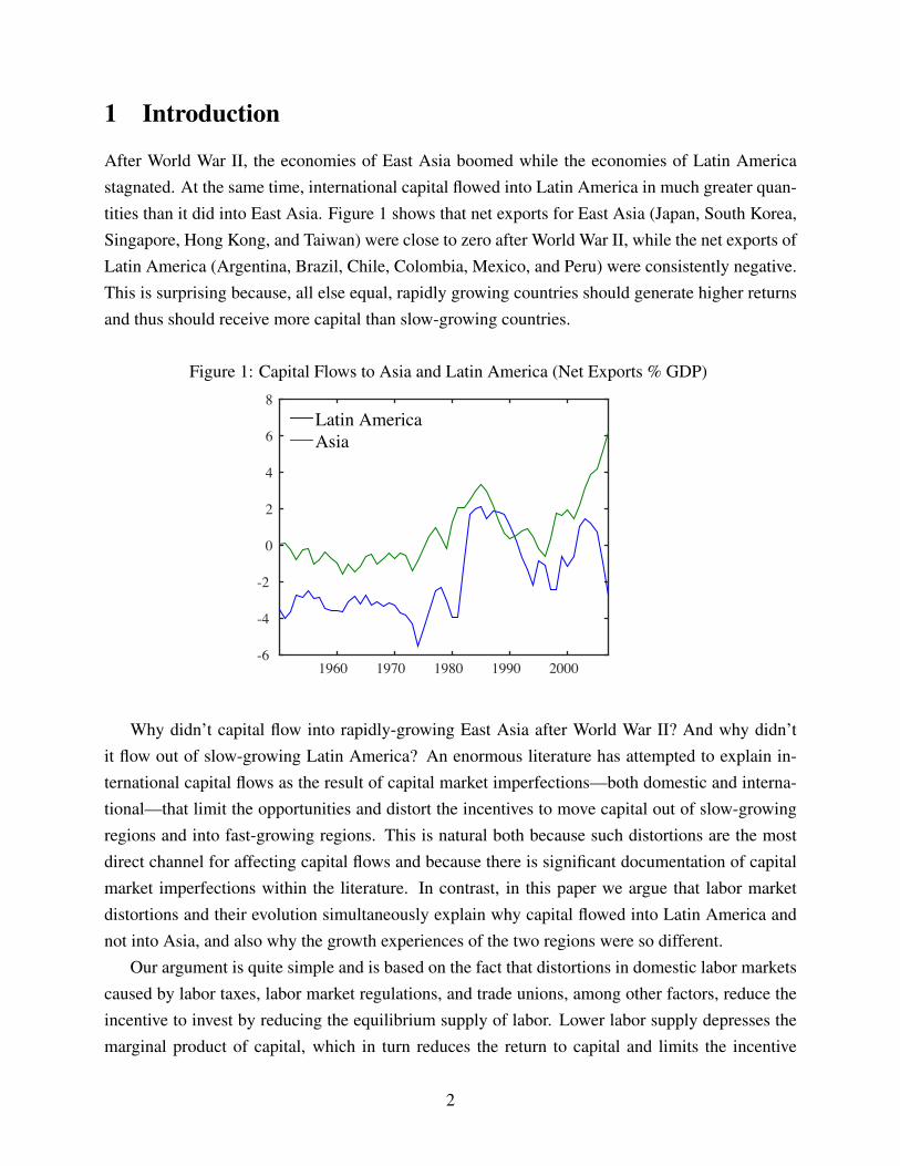
After World War II, the economies of East Asia boomed while the economies of Latin Americastagnated. At the same time, international capital flowed into Latin America in much greater quan-tities than it did into East Asia. Figure 1 shows that net exports for East Asia (Japan, South Korea,Singapore, Hong Kong, and Taiwan) were close to zero after World War II, while the net exports ofLatin America (Argentina, Brazil, Chile, Colombia, Mexico, and Peru) were consistently negative.This is surprising because, all else equal, rapidly growing countries should generate higher returnsand thus should receive more capital than slow-growing countries.

Figure 1: Capital Flows to Asia and Latin America (Net Exports % GDP)

1960 1970 1980 1990 2000-6

-4

-2

0

2

4

6

8Latin AmericaAsia

Why didn’t capital flow into rapidly-growing East Asia after World War II? And why didn’tit flow out of slow-growing Latin America? An enormous literature has attempted to explain in-ternational capital flows as the result of capital market imperfections—both domestic and interna-tional—that limit the opportunities and distort the incentives to move capital out of slow-growingregions and into fast-growing regions. This is natural both because such distortions are the mostdirect channel for affecting capital flows and because there is significant documentation of capitalmarket imperfections within the literature. In contrast, in this paper we argue that labor marketdistortions and their evolution simultaneously explain why capital flowed into Latin America andnot into Asia, and also why the growth experiences of the two regions were so different.

Our argument is quite simple and is based on the fact that distortions in domestic labor marketscaused by labor taxes, labor market regulations, and trade unions, among other factors, reduce theincentive to invest by reducing the equilibrium supply of labor. Lower labor supply depresses themarginal product of capital, which in turn reduces the return to capital and limits the incentive

2

for investment. This is particularly stark in the case of Asia, where hours worked per capita wererelatively low in 1950, grew rapidly in the succeeding decade, and then continued to rise moreslowly until the beginning of the 1990s. This suggests that labor market distortions were very highin 1950 and declined rapidly initially, with less-rapid declines thereafter. High and declining labormarket distortions thus help to explain both why Asia initially grew so fast as well as why growthleveled off after 1995, while the initially high level of these distortions explains why so little capitalflowed into the region immediately after World War II.

To the best of our knowledge, labor market distortions have not previously been studied asdeterminants of the pattern of capital flows. Consequently, the relative importance of labor versuscapital market distortions in understanding capital flows is an open question. Toward an answerto this question, this paper presents a capital flow accounting framework to quantitatively assessthe relative impact of capital and labor market distortions on the pattern of capital flows betweenEast Asia, Latin America, and the rest of the world (primarily Europe and North America) from1950 to 2007. Specifically, we construct a multi-country dynamic stochastic general equilibriummodel of the world economy augmented with “wedges” that affect the incentives to invest, work,and trade capital internationally. This framework builds on the (closed economy) business cycleaccounting framework of Cole and Ohanian (2002) and Chari, Kehoe, and McGrattan (2007) andextends it to an open economy setting through the introduction of an international wedge in which acountry-specific tax is applied to the purchase of international contingent claims. In contrast to thebusiness cycle accounting approach, we focus our analysis on lower frequency movements in thedata that influence the incentives to consume and save, and hence play a major role in determininginternational capital flows.

With the wedges added, the model can exactly replicate the data on economic outcomes inthe world economy, including world capital flows. We estimate the parameters of the model on anovel dataset of factor accumulation, employment, economic outcomes, and capital flows in LatinAmerica, East Asia, and the rest of the world and use the estimated model to recover the wedgesthat account for world capital flows. We compare movements in the resulting wedges to a narrativehistory of significant policy changes in these regions and argue that a significant component of themovements in the wedges is associated with fluctuations in government policies, thus leading us tointerpret the wedges structurally as policy distortions.

Our first finding is that the labor market distortions exhibit by far the most variation over time,changing by as much as 50 percent in all three regions. To assess the relative quantitative im-portance of labor market distortions in explaining capital flows over time, we then conduct coun-terfactual experiments that shut down movements in all of these distortions. We interpret theseexperiments as policy reforms. Our most striking finding from these experiments is that labor mar-ket distortions—rather than either international or domestic capital market distortions—have been

3

the single most important factor driving the pattern of capital flows for much of the postwar period.Specifically, domestic labor market distortions explain roughly 30 percent of the variation in capitalflows to Asia and Latin America during the 1950s and 1960s, while the general equilibrium effectsof labor market distortions in other regions account for another 30 to 40 percent in total. All told,the direct and indirect impact of labor market distortions account for about 60-70 percent of capitalflows to Asia and Latin America.

International capital market distortions also matter. The most surprising finding is that thesefluctuations have had their most significant impact in more recent decades, after many countriesliberalized international capital transactions, rather than in the 1950s and 1960s when these distor-tions were believed to be large. This finding primarily reflects the legacy of past distortions andtheir propagation through a country’s stock of net foreign assets, rather than the contemporaneouseffect of new distortions, with the exception of the Latin American debt crisis of the 1980s. We findthat the international capital market distortions operated to discourage capital inflows into Asia inthe 1950s. However, from the 1960s onward, and contrary to what is commonly believed, Asiancapital outflows would have been far greater if not for international capital market distortions. Do-mestic capital market distortions are found to have a quantitatively far less important impact oncapital flows throughout the postwar period.

The remainder of the paper is organized as follows. The next subsection discusses previousliterature. Section 2 presents the benchmark model economy and describes how the closed econ-omy wedge methodology used at business cycle frequencies is adapted to the open economy settingusing lower frequency data. Section 3 discusses the measurement of the wedges, our data sources,and our procedures for calibrating and estimating parameters. Section 4 presents our results. Sec-tion 5 discusses robustness and extensions, and Section 6 concludes. An online appendix collectsmore details on the material presented in the text.

1.1 Previous Literature

Our paper connects to four distinct but related literatures. First, the paper contributes to the verylarge literature that studies patterns in capital flows. This literature has largely been focused on howvarious capital market distortions affect flows. Indeed, much of the literature, following Feldsteinand Horioka’s (1980) examination of the correlation between domestic savings and investmentrates, has interpreted their analyses as “tests” of international capital market efficiency (see alsoBayoumi and Rose (1993), Taylor (1996), Tesar (1991), and many others). Responding to thefailures of these tests, the literature has responded by developing models of international financialfrictions ranging from limited commitment (Wright (2001), Kehoe and Perri (2002), and Restrepo-Echavarria (2018)) and default risk (Eaton and Gersovitz (1981), Arellano (2008), Aguiar and

4

Gopinath (2006), Tomz and Wright (2013), and many others) to exogenous market incompleteness(Bai and Zhang (2010)) and asymmetric information (Atkeson (1991)). A problem with these“tests” of capital mobility is that they typically rely on strong assumptions about the existenceand source of gains from trade, and hence these have low power against plausible alternatives asto the nature of the gains from trade. Our approach complements this literature on internationalfinancial market inefficiency by evaluating these frictions using a different framework that usesdata on a wider set of macroeconomic variables to simultaneously identify the sources of gainsfrom international trade in capital and to back out the potential role of distortions in limiting thattrade.

Our emphasis on measuring the gains from trade and in exploring the role of frictions outside ofcapital markets is shared by a number of other recent studies of international capital flows. Caselliand Feyrer (2007) directly estimate the marginal product of capital for many countries and find thatthese estimates have converged over time, once the marginal products are adjusted for the shareof non-reproducible capital, such as land and natural resources. They conclude on the basis ofthis convergence that the gains from international trade in capital have declined, implying that anyinternational capital market distortions have become less important over time.1

We explore the connection of their results to our own below in Subsection 4.3.1. Obstfeld andRogoff (2001), Fitzgerald (2012), Reyes-Heroles (2016), Eaton, Kortum, and Neiman (2016), andothers explore the role of trade costs in explaining a number of facts about international flows. Weargue that our approach is complementary in that it provides evidence that can be used to test forthe role of trade costs, although we argue in Section 5 that our findings suggest a relatively minorrole for these costs in explaining the relative allocation of capital flows between Asia and LatinAmerica.

We follow in the footsteps of Alfaro, Kalemli-Ozcan, and Volosovych (2008), who study therole of institutions in driving the incentive to reallocate capital around the world. Unlike them, wefocus on labor market institutions that depress labor supply and lower the return to capital as thekey factor. Alfaro, Kalemli-Ozcan, and Volosovych (2014) study the difference between officialand private capital flows since 1970 and find that private flows are more closely in accordancewith standard models than are official flows. This relies on significant departures from Ricardianequivalence to explain why private flows do not offset official flows in order to produce aggregatecapital flows in line with the theory. Below in Section 5, we argue that our approach yields evidenceas to the kind of departure that might be relevant in the data. Aguiar and Amador (2016) provide amodel of one such mechanism.

Second, our paper makes contact with the literature on East Asian growth and the debate as to1Ohanian and Wright (2008) and Monge-Naranjo, Sanchez, and Santaeulalia-Llopis (2015) extend the Caselli and

Feyrer (2007) approach and propose alternative methods for estimating the marginal product of physical capital.

5

the relative contribution of factor accumulation (see Young (1995)) and productivity growth (seeHsieh (1999)) in explaining East Asia’s rapid growth. We argue that incorporating data on interna-tional capital flows, and understanding the causes of the observed rapid factor accumulation, helpto shed light on this debate. Specifically, we find evidence for substantial distortions in East Asianlabor markets in the 1950s that both depressed returns to investment, limiting the incentive for in-ternational capital inflows, and, as the distortions were unwound, drove rapid factor accumulationand economic growth thereafter.

Third, our paper builds on the literature on business cycle accounting in closed economies fol-lowing Cole and Ohanian (2002) and Chari, Kehoe, and McGrattan (2007). Unlike these papers,we examine open economies and focus on medium- and longer-term movements in economic vari-ables, which play a larger role in determining the level of consumption, and hence also savings andinternational capital flows, than do fluctuations at business cycle frequencies. Our paper is alsorelated to the literature on business cycle accounting in small open economies (see Lama (2011)and Rahmati and Rothert (2014)). In contrast to their partial equilibrium (small open economy)approach with incomplete markets, we show how to apply a general equilibrium complete marketsmodel to data on the world economy constituted from multiple countries.

A related approach, and the paper perhaps most closely related to ours, is Gourinchas andJeanne (2013), which studies capital flow data from 1980 to 2000 for individual countries us-ing wedges in a deterministic open economy growth model without transitional dynamics. Theyalso abstract from labor supply decisions and so are unable to address the importance of the laborwedge. We discuss the differences between our analysis and that of Gourinchas and Jeanne (2013)in greater detail in Subsection 4.3.2 below. For now, we simply note that in comparison we empha-size capital flows during the decades from 1950 to 1970, and that our dynamic out-of-steady-stateanalysis allows us to study the impact of movements in the labor wedge, which chiefly matter outof steady-state.

Fourth and finally, our paper complements the large literature seeking to identify the presenceof distortions to factor markets both at home and abroad. Much of this literature computes indicesof distortions by examining legal restrictions on the operation of markets and then counting up thenumber of different types of restrictions. As such they provide a qualitative measure of the pres-ence of restrictions that are “on the books” (de jure). Examples of this approach in internationalcapital markets include the large number of studies based on the International Monetary Fund’sAnnual Report on Exchange Arrangements and Exchange Restrictions, including Chinn and Ito(2001), Quinn (1997), and many others, while examples covering domestic labor markets and cap-ital markets are cited below. As is openly acknowledged, these measures have two problems. First,some restrictions that are on the books may not be enforced in practice, while some restrictions thatare in practice may not appear on the books (a de jure restriction may not be a de facto restriction

6

and vice versa). Second, ultimately we are more interested in the quantitative significance of suchcontrols than we are in a qualitative measure of their presence. By contrast, our paper uses data onequilibrium quantities to construct quantitative measures of the impact of de facto restrictions oninternational and domestic capital markets as well as domestic labor markets that we believe serveas a useful complement to these qualitative de jure measures.

2 Capital Flow Accounting

As noted in the introduction, the existing literature has focused on distortions in capital markets,both domestic and international, in explaining anomalous international capital flows. In contrast,we hypothesize that labor market distortions played an important role in determining capital flows.In situations like this with a clear substantive question, many possible theories, and no canonicalanswer, it is productive to adopt an approach capable of identifying possible explanatory channelsand quantifying their significance. Hence, we develop a capital flow accounting framework. Ourmethod is a direct descendant of the closed economy business cycle accounting approaches of Coleand Ohanian (2002) and Chari, Kehoe, and McGrattan (2007) extended to the general equilibriumof a world economy. Unlike this earlier literature, which focuses on business cycle fluctuations inmacroeconomic variables, we are also interested in medium- and long-term frequencies that playa large role in determining capital flows and hence pay particular attention to long-run trends invariables.

Also unlike this literature, we start with a variant on the class of models typically used toanalyze international capital flows (for example, Mendoza (1991) and Baxter and Crucini (1993,1995)). We refer to this as our benchmark model and augment it with wedges so that it is able toexactly replicate the data on macroeconomic outcomes including capital flows. These wedges aredescribed as taxes that distort the marginal conditions determining optimal labor supply, domesticinvestment, and foreign investment but stand in for a wider range of departures from our benchmarkaccounting framework. We explore alternative interpretations of these wedges in Section 5 below.

2.1 Households

Consider a world economy composed of three “countries” indexed by j, where j = L stands for“Latin America,” j = A stands for “(East) Asia,” and j = R stands for the “rest of the world.” Timeevolves discretely and is indexed by t = 0,1, ..., so that Njt denotes the population of country jat time t. The decisions of each country are made by a representative agent with preferences over

7

consumption Cjt and per capita hours worked h jt ordered by

E0

"•

Ât=0

b t⇢

ln✓

Cjt

Njt

◆� j

1+ gh1+g

jt

�Njt

#.

The parameters governing preferences—the discount factor b , the preference for leisure j, and theFrisch elasticity of labor supply 1/g—are assumed common across countries; therefore, any cross-country differences in core preferences will hence be attributed to the wedges that we introducenext. We discuss how this assumption affects our results in Subsection 5.1 below.

The problem of the representative agent of country j is to choose a state-contingent stream ofconsumption levels Cjt , hours worked h jt , purchases of capital to be rented out next period Kjt+1,

and a portfolio of state-contingent international bond holdings B jt+1 subject to a sequence of flowbudget constraints for each state and date:

Cjt +PKjt Kjt+1 +Et

⇥qt+1B jt+1

⇤

⇣1� th

jt

⌘Wjth jtNjt +

�1� tB

jt�

B jt +Tjt

+�1� tK

jt��

rKjt +P⇤K

jt�

Kjt +P jt ,

with initial capital Kj0 and bonds B j0 given. Here Wjt is the wage per hour worked, rKjt the rental

rate of capital, PKjt the price of new capital goods, and P⇤K

jt the price of old capital goods, whichwill differ from the price of new capital goods due to the presence of adjustment costs in capital.In this complete markets environment, the prices of state-contingent international bonds at time tthat pay off in one state at t +1 are composed of a risk-adjusted world price qt+1 multiplied by theprobability of the state occurring, which allows us to write the expected value of the risk-adjustedexpenditures on bonds on the left-hand side of the flow budget constraint. Households also receiveprofits P jt from their ownership of domestic firms.

The t represent taxes or “wedges” on factor payments and investment income. Specifically,th is a tax on wage income (the labor wedge), tB is a tax on income derived from internationalassets or, equivalently, a subsidy on the cost of paying for international liabilities (the internationalwedge), while tK is a tax on income from domestic capital (the capital wedge). Any revenue fromthese taxes net of the level of government spending G jt are assumed to be transferred in lump-sumfashion to or from households each period as Tjt ,

Tjt = thjtWjth jtNjt + tB

jtB jt + tKjt�rK

jt +P⇤Kjt�

Kjt �G jt . (1)

This implies that there is no government borrowing. As Ricardian equivalence holds in our model,this is without loss of generality. However, some authors (for example, Alfaro, Kalemli-Ozcan,and Volosovych (2014)) have argued that an understanding of government borrowing is necessary

8

to rationalize observed capital flows. We discuss these issues in more detail in Subsection 5.3below.

The first-order conditions for the household can be rearranged to find the optimal conditiongoverning the labor supply, ⇣

1� thjt

⌘Wjt

Njt

Cjt= jhg

jt , (2)

the Euler equation for domestic capital,

1 = Et

"b

Cjt/Njt

Cjt+1/Njt+1

�1� tK

jt+1� rK

jt+1 +P⇤Kjt+1

PKjt

#, (3)

and the Euler equation for state-contingent international assets,

Cjt+1/Njt+1

Cjt/Njt=

bq�1� tB

jt+1�. (4)

Although our focus is on capital flows, which are influenced by economic fluctuations at short-,medium-, and long-run frequencies, our framework shares a number of elements with the closedeconomy business cycle accounting literature (see Cole and Ohanian (2002) and Chari, Kehoe, andMcGrattan (2007)). However, while the labor and capital wedges are familiar, the internationalwedge is new and has been added to create an open economy accounting framework. This termdrives a wedge between the growth rate of the domestic marginal utility of consumption and thereturn on international assets. It differs from the way international factors are subsumed into theclosed economy framework of Chari, Kehoe, and McGrattan (2007), where net exports are treatedas an additive output shock equivalent to government expenditure.

2.2 Firms

Each country is populated by two types of firms. The first type of firm hires labor and cap-ital to produce the consumption good using a standard Cobb-Douglas technology of the formA jtKa

jt�h jtNjt

�1�a , where A jt is the level of aggregate productivity in the economy and a is theoutput elasticity of capital. This yields expressions for the equilibrium wage rate per hour and therental rate on capital:

Wjt = (1�a)Yjt

h jtNjt, and rK

jt = aYjt

Kjt. (5)

The second type of firm produces new capital goods Kjt+1 using Xjt units of investment (de-ferred consumption) and Kjt units of the old capital good. Their objective is to maximize profitsPK

jt Kjt+1 �Xjt �P⇤Kjt Kjt subject to the capital production function (or capital accumulation equa-

9

tion) with convex adjustment costs f of the form

Kjt+1 = (1�d )Kjt +Xjt �f✓

Xjt

Kjt

◆Kjt .

Note that, although the capital good Kjt+1 is to be used for production in period t+1, it is producedand sold in period t at price PK

jt . This gives rise to first-order conditions:

PKjt =

1

1�f 0⇣

XjtKjt

⌘ , (6)

P⇤Kjt = PK

jt

✓1�d �f

✓Xjt

Kjt

◆+f 0

✓Xjt

Kjt

◆Xjt

Kjt

◆. (7)

We assume that adjustment costs are of the quadratic form:

f✓

Xjt

Kjt

◆=

n2

✓Xjt

Kjt�k◆2

.

All production parameters—the output elasticity of capital a, the depreciation rate d , and thosegoverning adjustment costs n and k—are assumed constant across countries; we return to thisassumption in Section 5.1 below.

2.3 Growth and Uncertainty

The world economy has grown substantially over the period under study. But this growth is not wellrepresented by movements around a deterministic trend with a constant growth rate. Moreover,expectations of future growth in income drive a household’s desire to save and invest and henceplay a large role (in many cases, the dominant role) in determining capital flows. Hence, it is notappropriate to simply apply the Hodrick-Prescott filter to the data and proceed with a detrendedmodel, as might be done for a business cycle accounting analysis. As a consequence, we adopt aspecification for the growth of the population and productivity level in each country that allows thedata to speak to us about these expectations of future trends.

We assume that there is a stochastic world trend for both population and productivity andassociate this with growth in the rest of the world (for similar approaches, see Canova (1998),Fernandez-Villaverde and Rubio-Ramirez (2007), and Cheremukhin and Restrepo-Echavarria (2014)).Specifically, we assume that the rest of the world productivity and population evolve according to

lnARt+1 = lnARt + lnpss +sAR eA

Rt ,

lnNRt+1 = lnNRt + lnhss +sNR eN

Rt ,

10

where pss and hss are the growth rates in world productivity and population that would occur in thedeterministic steady-state of our model. The parameters sA

R and sNR govern the volatility of these

stochastic trends. In order to make our model of the world economy stationary, we scale by thelevel of effective labor in the rest of the world Zt = A1/(1�a)

Rt NRt . Note that our specification nests aconstant growth rate as a special case.

Population and productivity levels in Asia and Latin America are assumed to evolve relativeto the world trend in such a way that a non-degenerate long-run distribution of economic activityacross countries is preserved. Specifically, for Asia and Latin America we define relative produc-tivity a jt = A jt/ARt and relative population n jt = Njt/NRt and assume that both a jt and n jt followfirst-order autoregressive processes of the form

lna jt+1 =�1�ra

j�

lna jss +raj lna jt +sa

j eajt+1,

lnn jt+1 =�1�rn

j�

lnn jss +rnj lnn jt +sn

j enjt+1.

This allows for long-lasting deviations from the world trend. We place no further restrictions onthese processes, preferring to allow the data to speak by estimating their parameters directly.

The labor, capital, and international wedges (indexed by m = h,K, and B) for each country arealso assumed to follow univariate first-order autoregressive processes of the form

ln�1� tm

jt+1�=�1�rm

j�

ln�1� tm

jss�+rm

j ln�1� tm

jt�+sm

j emjt+1, (8)

where tmjss is the level the wedge would take on in the deterministic steady-state of our model

and rmj governs the rate of mean reversion. The evolution of the level of government spending in

each country G jt is assumed to be such that the ratio of government spending to national incomeg jt = G jt/Yjt also follows a first-order autoregressive process:

lng jt+1 =⇣

1�rgj

⌘lng jss +rg

j lng jt +sgj eg

jt+1.

The parameters of all of these processes, with the exception of the steady-state international wedgeto be discussed next, are estimated from, or calibrated to, match the data.

2.4 Model Solution

Our benchmark assumes that the world economy has complete markets. Complete markets are anatural benchmark, as there are many ways in which markets can be incomplete. It is also thenatural approach to modeling a world economy with very rich and complex asset trades—certainlymore assets than can be accommodated in a tractable incomplete markets model. However, given

11

our continuous state space, this means that each country has an infinite dimensional portfolio deci-sion to make each period. In a contribution that may be of independent interest, we establish thatthe solution to a particular pseudo social planner’s problem corresponds to the equilibrium of ourcomplete markets economy and work directly on the pseudo social planner’s problem. Appendix Adescribes in detail the mapping between the competitive equilibrium problem and the pseudo socialplanner’s problem. As noted earlier, to obtain stationarity, we scale by the stochastic world trendZt�1 to obtain an intensive form version of the model.

The large number of state variables (23) leads us to use perturbation methods. To do so, wemake additional assumptions to ensure that the model has a unique non-degenerate deterministicsteady-state (which serves as the point about which the approximation is taken). To see the needfor these assumptions, note that for our reference country R and any other country j, we can takeequation (4) and rearrange to obtain the first equality in

Cjt+1/Njt+1

CRt+1/NRt+1=

Cjt/Njt

CRt/NRt

1� tBjt+1

1� tBRt+1

=Cjt/Njt

CRt/NRt

�1� tB

jt+1�. (9)

This means we cannot separately identify each country’s international wedge tBj , and so we nor-

malize the rest of the world international wedge to zero, tBRt+1 = 0, yielding the second equality. It

also means that, if the steady-state international wedge, tBjss, is not equal to zero, there is a long-run

trend in relative consumption levels so that the deterministic steady-state distribution of consump-tion is degenerate (one country’s share of consumption must converge to zero). Moreover, simplyassuming that tB

jss = 0 for all j does not pin down a unique steady-state relative consumption level.Intuitively, the level of the international wedge out of steady-state affects the accumulation of in-ternational assets, which in turn affects long-run consumption levels. In terms of equation (9), thegrowth rate of relative consumption is a first-order autoregressive process that converges to zero inthe deterministic steady-state; the long-run level of relative consumption depends upon the entiresequence of realizations of the international wedge.

Analogous issues arise in multi-agent models with heterogeneous rates of time preference (seethe conjecture of Ramsey (1928), the proof of Becker (1980), and the resolution of Uzawa (1968))and in small open economy incomplete markets models. In the latter context, a suite of alternativeresolutions of this issue have been proposed (see Schmitt-Grohe and Uribe (2003) for a survey anddiscussion). We use a variant of the portfolio adjustment cost approach, adapted to our generalequilibrium complete markets setting. Specifically, for Asia and Latin America, we assume thattheir international wedges can be decomposed into a pure tax on international investment incomet⇤B

jt and another term Y jt , both of which the country takes as given:

1� tBjt = 1� t⇤B

jt +Y jt .

12

We refer to t⇤B as the international wedge from now on (typically suppressing the asterisk) andassume that it follows a first-order autoregressive process with the steady-state assumed to be zero:

ln�1� t⇤B

jt+1�= rB

j ln�1� t⇤B

jt�+sB

j eBjt+1. (10)

The other term takes the form of a portfolio tax that is assumed, in equilibrium, to satisfy

Y jt =�1� t⇤B

jt�"✓

Cjt/Njt

CRt/NRt

1y j0

◆�y j1

�1

#. (11)

This ensures that, in the deterministic steady-state, relative consumption levels are pinned down byy j0, with mean reversion in relative consumption levels controlled by y jt as

lnCjt+1/Njt+1

CRt+1/NRt+1=

y j1

1+y j1lny j0 +

11+y j1

lnCjt/Njt

CRt/NRt+

11+y j1

ln�1� t⇤B

jt+1�. (12)

We refer to this as a portfolio tax because in steady-state, relative consumption levels map one-for-one into net foreign asset positions. Once again, these parameters are identified from the data,meaning that we allow the data to estimate the long-run net foreign asset position of each country.

Under these assumptions on the portfolio tax, there exists a unique non-degenerate deterministicsteady-state. We proceed by taking a first-order log-linear approximation of the pseudo socialplanner’s problem around this point.

3 Implementation

The multi-country dynamic stochastic general equilibrium model of the world economy augmentedwith wedges described above has been designed to exactly replicate data on the national incomeand product account expenditure aggregates. In this sense, the model can be used as an accountingframework for observed data. In this section, we describe how the model uses these data to identifythe wedges. We then briefly describe our data sources, with a more detailed discussion availablein Appendix B. To recover realizations of the capital wedge, we must compute the equilibrium ofthe model in order to determine expectations of future returns to capital, and so we also describeour solution method. A small number of structural parameters governing preferences and produc-tion are calibrated. Some wedges can be recovered, and the parameters governing their evolutionestimated, without solving the model. The remaining parameters of the model are estimated usingBayesian methods.

13

3.1 Using the Data to Measure the Wedges

Realizations of the labor, capital, and international wedges can all be measured by feeding dataon the national income and accounting expenditure aggregates through the optimality conditionsof households and firms combined with the equilibrium conditions of the model. Realizations ofthe labor and international wedges can be computed directly from first-order conditions withoutknowing the solution of the model. The capital wedge, on the other hand, requires the computationof expectations about future capital returns and hence requires both estimating and solving themodel.

To see this, note that under our assumption of complete markets, the composite internationalwedge and portfolio tax tB

jt+1 can be recovered from data on the growth in relative consumptionlevels, as shown in equation (9). Estimation of equation (12) serves to both decompose the com-posite into the international wedge t⇤B

jt+1 and the portfolio tax Y jt+1 and estimate the parametersgoverning the evolution of the international wedge and the portfolio tax. Note that under the as-sumptions of our model, the residual in this equation—the international wedge—follows an autore-gressive process; relative consumption does not follow a simple first-order autoregressive process.Nonetheless, all that is needed to estimate the process governing the international wedge and theparameters of the portfolio tax is data on the growth in relative consumption levels. This can bedone without solving the entire model.

The labor wedge can also be recovered, and its evolution process estimated, outside of themodel. Specifically, using the optimal labor supply condition for the household (2) and the optimalemployment decision of the firm (5), we obtain

1� thjt =

j1�a

hgjt

h jtNjt

Yjt

Cjt

Njt. (13)

That is, using data on consumption, population, hours worked, and output, and given values forthe production and preference parameters, we can recover realizations of the labor wedge withoutsolving the model. This can then be used to estimate the process governing the evolution of thelabor wedge. Note that it is not possible to separately identify the level of the labor wedge from thepreference for leisure parameter j , which in principle could also vary across countries. Hence, inwhat follows, we normalize the leisure parameter to 1 for all countries, and we focus on changes inthe levels of these wedges over time, and not on cross-country differences in their levels.

Lastly, the capital wedge is determined from the Euler equation for the household (3), theoptimal capital decision of the consumer good firm (5), and the optimality conditions of the capitalgood firm (6) and (7). Denoting by x jt+1 = Xjt+1/Kjt+1 the ratio of investment to the capital stock,

14

we obtain the capital wedge from

1 = Et

2

64bCjt+1/Njt+1

Cjt/Njt

�1� tK

jt+1� a Yjt+1

Kjt+1+

1�d�f(x jt+1)+f 0(x jt+1)x jt+1

1�f 0(x jt+1)1

1�f 0(x jt)

3

75 . (14)

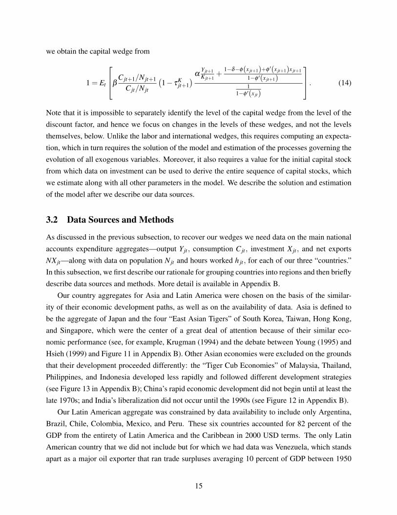
Note that it is impossible to separately identify the level of the capital wedge from the level of thediscount factor, and hence we focus on changes in the levels of these wedges, and not the levelsthemselves, below. Unlike the labor and international wedges, this requires computing an expecta-tion, which in turn requires the solution of the model and estimation of the processes governing theevolution of all exogenous variables. Moreover, it also requires a value for the initial capital stockfrom which data on investment can be used to derive the entire sequence of capital stocks, whichwe estimate along with all other parameters in the model. We describe the solution and estimationof the model after we describe our data sources.

3.2 Data Sources and Methods

As discussed in the previous subsection, to recover our wedges we need data on the main nationalaccounts expenditure aggregates—output Yjt , consumption Cjt , investment Xjt , and net exportsNXjt—along with data on population Njt and hours worked h jt , for each of our three “countries.”In this subsection, we first describe our rationale for grouping countries into regions and then brieflydescribe data sources and methods. More detail is available in Appendix B.

Our country aggregates for Asia and Latin America were chosen on the basis of the similar-ity of their economic development paths, as well as on the availability of data. Asia is defined tobe the aggregate of Japan and the four “East Asian Tigers” of South Korea, Taiwan, Hong Kong,and Singapore, which were the center of a great deal of attention because of their similar eco-nomic performance (see, for example, Krugman (1994) and the debate between Young (1995) andHsieh (1999) and Figure 11 in Appendix B). Other Asian economies were excluded on the groundsthat their development proceeded differently: the “Tiger Cub Economies” of Malaysia, Thailand,Philippines, and Indonesia developed less rapidly and followed different development strategies(see Figure 13 in Appendix B); China’s rapid economic development did not begin until at least thelate 1970s; and India’s liberalization did not occur until the 1990s (see Figure 12 in Appendix B).

Our Latin American aggregate was constrained by data availability to include only Argentina,Brazil, Chile, Colombia, Mexico, and Peru. These six countries accounted for 82 percent of theGDP from the entirety of Latin America and the Caribbean in 2000 USD terms. The only LatinAmerican country that we did not include but for which we had data was Venezuela, which standsapart as a major oil exporter that ran trade surpluses averaging 10 percent of GDP between 1950

15

and 1975 (see Figure 14 in Appendix B). The rest of the world aggregates data from 22 advancedeconomies in North America, Europe, and Oceania, which are described in more detail in AppendixB. Appendix B also plots the resulting data series that are used in the estimation.

Data were obtained from a number of sources. Briefly, where available, data from the Organi-sation for Economic Co-operation and Development were used for its member countries. For othercountries, data from the World Bank’s World Development Indicators were our primary source.Data prior to 1960 were typically taken from the World Bank’s World Tables of Economic and So-cial Indicators. The Groningen Growth and Development Center was a valuable source of hoursworked data. Gaps in the resulting database were filled using a number of other sources as de-tailed in the online appendix. A small number of missing observations are replaced using dataextrapolated or interpolated from other countries in the relevant country aggregate. For the purposeof comparing our model-generated estimates of the level of productivity and capital stocks to thedata, we use the estimate of capital stocks in 1950 from Nehru and Dhareshwar (1993) combinedwith the perpetual inventory method to construct a reference series for the capital stock and theimplied level of productivity. Appendix B provides a detailed country-by-country description ofdata sources.

All national accounts data were transformed to constant 2000 USD prices. Data were aggre-gated by summation for each region. Net exports for the rest of the world were constructed toensure that the world’s trade balance with itself was zero, and any statistical discrepancy for aregion was added to government spending.

3.3 Calibration and Estimation

As noted above, we solve the model numerically by taking a first-order log-linear approximationof the model around its deterministic steady-state, which is well defined under our assumptionson the portfolio tax. After imposing symmetry in the preference and production parameters acrosscountries, we must assign values to 68 parameters. In this subsection, we describe how someparameters are calibrated to standard values and others are estimated outside the model, while theremainder are estimated by Bayesian methods using the Kalman filter.

The parameters governing preferences and production are assumed constant across countries,so that any differences across countries are attributed to the wedges. Of these common parameters(collected in Table 1), six are calibrated to standard values, while a seventh is a normalization.Specifically, we set the output elasticity of capital in the Cobb-Douglas production function a to0.36, the discount factor b to 0.96, and the depreciation rate d to 7 percent per year. These areall standard values. The curvature for the disutility of labor g is set to 1.5, which implies a Frischelasticity of labor supply of two-thirds. This is within the range typically estimated using micro

16

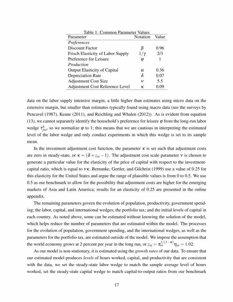
Table 1: Common Parameter ValuesParameter Notation ValuePreferencesDiscount Factor b 0.96Frisch Elasticity of Labor Supply 1/g 2/3Preference for Leisure j 1ProductionOutput Elasticity of Capital a 0.36Depreciation Rate d 0.07Adjustment Cost Size n 5.5Adjustment Cost Reference Level k 0.09

data on the labor supply intensive margin, a little higher than estimates using micro data on theextensive margin, but smaller than estimates typically found using macro data (see the surveys byPencavel (1987), Keane (2011), and Reichling and Whalen (2012)). As is evident from equation(13), we cannot separately identify the household’s preference for leisure j from the long-run laborwedge th

jss, so we normalize j to 1; this means that we are cautious in interpreting the estimatedlevel of the labor wedge and only conduct experiments in which this wedge is set to its samplemean.

In the investment adjustment cost function, the parameter k is set such that adjustment costsare zero in steady-state, or k = (d + zss �1) . The adjustment cost scale parameter n is chosen togenerate a particular value for the elasticity of the price of capital with respect to the investment-capital ratio, which is equal to nk. Bernanke, Gertler, and Gilchrist (1999) use a value of 0.25 forthis elasticity for the United States and argue the range of plausible values is from 0 to 0.5. We use0.5 as our benchmark to allow for the possibility that adjustment costs are higher for the emergingmarkets of Asia and Latin America; results for an elasticity of 0.25 are presented in the onlineappendix.

The remaining parameters govern the evolution of population, productivity, government spend-ing; the labor, capital, and international wedges; the portfolio tax; and the initial levels of capital ineach country. As noted above, some can be estimated without knowing the solution of the model,which helps reduce the number of parameters that are estimated within the model. The processesfor the evolution of population, government spending, and the international wedges, as well as theparameters for the portfolio tax, are estimated outside of the model. We impose the assumption thatthe world economy grows at 2 percent per year in the long run, or zss = p1/(1�a)

ss hss = 1.02.As our model is non-stationary, it is estimated using the growth rates of our data. To ensure that

our estimated model produces levels of hours worked, capital, and productivity that are consistentwith the data, we set the steady-state labor wedge to match the sample average level of hoursworked, set the steady-state capital wedge to match capital-to-output ratios from our benchmark

17

capital series, and estimate the steady-states and persistence of the productivity processes from ourbenchmark productivity series.

All other parameters are then estimated using Bayesian methods (see An and Schorfheide(2007)). Our decision to use Bayesian methods is a pragmatic one; our use of standard prior distri-butions serves to focus the estimation on the “right” region of the parameter space. Our choices arecollected in Appendix C along with the plots of the prior and posterior distributions, which showthat our chosen priors are not restrictive with the estimated parameters reflecting the informationcontained in the data.

The linearized equations of the model combined with the linearized measurement equationsform a state-space representation of the model. We apply the Kalman filter to compute the likeli-hood of the data given the model and to obtain the paths of the wedges. We combine the likelihoodfunction L

�Y Data|p

�, where p is the parameter vector, with a set of priors p0 (p) to obtain the pos-

terior distribution of the parameters p�

p|Y Data� = L�Y Data|p

�p0 (p). We use the random-walk

Metropolis-Hastings implementation of the MCMC algorithm to compute the posterior distribu-tion.

The point values for each of our parameters are collected in Table 2. The estimates implythat long-run population growth of the world is roughly 0.67 percent per year. In the long run, it isestimated that the population of Latin America will exceed that in the rest of the world aggregate by13 percent, while in East Asia the population will settle down to 29 percent of the rest of the worldlevel. Productivity, on the other hand, will converge to 37 percent of the rest of the world level inLatin America and to 77 percent of that level in Asia. Under our assumption of 2 percent long-rungrowth, the long-run growth of productivity settles down to 0.85 percent per year, or pss = 1.0085.Productivity and population are very persistent in all regions. Government expenditure stabilizesat between 12 percent (Asia) and 19 percent (rest of the world) of GDP and is estimated to be quitepersistent.

The long-run level of the labor wedge cannot be separately identified from a country’s prefer-ence for leisure parameter j. After normalizing j = 1 for all countries, the long-run labor wedgeis found to be positive for Asia and the rest of the world and negative for Latin America, indi-cating that average hours worked in Latin America are larger than predicted from implied wagesand consumption levels and hence must require a subsidy. Of course, this could simply reflectdifferences in preferences: perhaps people in Latin American have a lower preference for leisure?In order to avoid being drawn into debates on this question, we focus our attention on changes inthese measured wedges over time rather than cross-country differences in their levels. Likewise,the steady-state levels of the capital wedge cannot be separately identified from the discount factor.Given our normalization for b , all long-run capital wedges are small and are approximately zero inAsia.

18

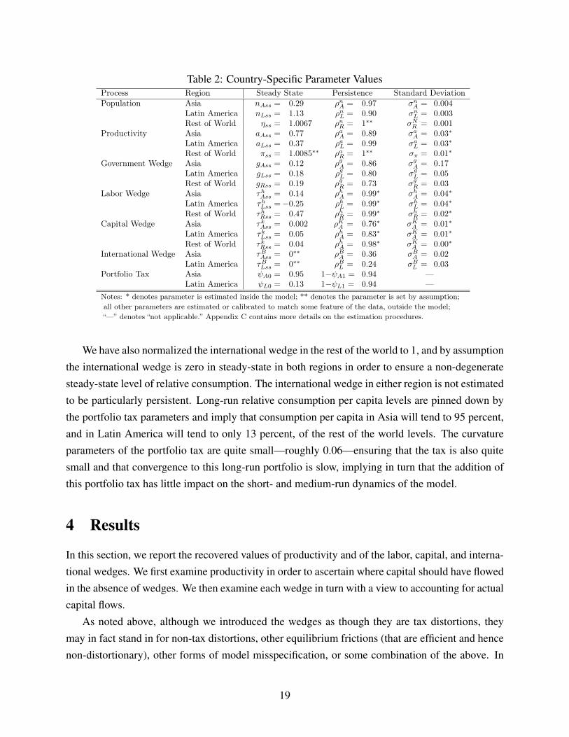
Table 2: Country-Specific Parameter ValuesProcess Region Steady State Persistence Standard DeviationPopulation Asia nAss = 0.29 ⇢nA = 0.97 �n

A = 0.004Latin America nLss = 1.13 ⇢nL = 0.90 �n

L = 0.003Rest of World ⌘ss = 1.0067 ⇢nR = 1⇤⇤ �N

R = 0.001Productivity Asia aAss = 0.77 ⇢aA = 0.89 �a

A = 0.03⇤

Latin America aLss = 0.37 ⇢aL = 0.99 �aL = 0.03⇤

Rest of World ⇡ss = 1.0085⇤⇤ ⇢aR = 1⇤⇤ �⇡ = 0.01⇤

Government Wedge Asia gAss = 0.12 ⇢gA = 0.86 �gA = 0.17

Latin America gLss = 0.18 ⇢gL = 0.80 �gL = 0.05

Rest of World gRss = 0.19 ⇢gR = 0.73 �gR = 0.03

Labor Wedge Asia ⌧hAss = 0.14 ⇢hA = 0.99⇤ �hA = 0.04⇤

Latin America ⌧hLss =�0.25 ⇢hL = 0.99⇤ �hL = 0.04⇤

Rest of World ⌧hRss = 0.47 ⇢hR = 0.99⇤ �hR = 0.02⇤

Capital Wedge Asia ⌧kAss = 0.002 ⇢KA = 0.76⇤ �KA = 0.01⇤

Latin America ⌧kLss = 0.05 ⇢hA = 0.83⇤ �KA = 0.01⇤

Rest of World ⌧kRss = 0.04 ⇢hA = 0.98⇤ �KA = 0.00⇤

International Wedge Asia ⌧BAss = 0⇤⇤ ⇢BA = 0.36 �BA = 0.02

Latin America ⌧BLss = 0⇤⇤ ⇢BL = 0.24 �BL = 0.03

Portfolio Tax Asia A0 = 0.95 1� A1 = 0.94 —Latin America L0 = 0.13 1� L1 = 0.94 —

Notes: * denotes parameter is estimated inside the model; ** denotes the parameter is set by assumption;all other parameters are estimated or calibrated to match some feature of the data, outside the model;“—” denotes “not applicable.” Appendix C contains more details on the estimation procedures.

1

We have also normalized the international wedge in the rest of the world to 1, and by assumptionthe international wedge is zero in steady-state in both regions in order to ensure a non-degeneratesteady-state level of relative consumption. The international wedge in either region is not estimatedto be particularly persistent. Long-run relative consumption per capita levels are pinned down bythe portfolio tax parameters and imply that consumption per capita in Asia will tend to 95 percent,and in Latin America will tend to only 13 percent, of the rest of the world levels. The curvatureparameters of the portfolio tax are quite small—roughly 0.06—ensuring that the tax is also quitesmall and that convergence to this long-run portfolio is slow, implying in turn that the addition ofthis portfolio tax has little impact on the short- and medium-run dynamics of the model.

4 Results

In this section, we report the recovered values of productivity and of the labor, capital, and interna-tional wedges. We first examine productivity in order to ascertain where capital should have flowedin the absence of wedges. We then examine each wedge in turn with a view to accounting for actualcapital flows.

As noted above, although we introduced the wedges as though they are tax distortions, theymay in fact stand in for non-tax distortions, other equilibrium frictions (that are efficient and hencenon-distortionary), other forms of model misspecification, or some combination of the above. In

19

other words, the recovered wedges may be reduced-form representations of diverse structural phe-nomena, rather than true primitives of the model. Moreover, a structural distortion in one factormarket may be recovered as a reduced-form wedge affecting another factor market or even the levelof productivity. We view this as a virtue of the approach, as it pinpoints the precise margins—theallocation of time between market and non-market activities, or the allocation of resources betweenconsumption and investment at home and abroad—that drive observed capital flows in a way thatcan be informative about large classes of structural models.

Nonetheless, toward a structural interpretation of these wedges, we present our findings on thebehavior of the recovered wedges in parallel with a narrative history of factor market distortionsin Latin America and Asia. We show that movements in our recovered wedges are often associ-ated with changes in both quantitative and qualitative changes in measures of both tax and non-taxregulatory distortions. This leads us to a structural interpretation of the wedges as reflecting pol-icy distortions affecting factor markets. With this structural interpretation in hand, we carry outcounterfactual exercises to assess the relative importance of labor market, domestic capital market,and international capital market distortions. Our interest is in the answer to the following ques-tion: Given the evolution of productivity growth across countries, why didn’t more capital flowinto Asia and out of Latin America? As a result, we take the evolution of productivity as given inour counterfactual experiments.

4.1 The Evolution of Productivity and the Wedges

4.1.1 Productivity

Our estimates of total factor productivity across the three regions (A jt) are depicted in Figure 2.The solid lines represent the realizations of the wedges, while the dashed segments represent theforecast implied by the stochastic process of each of the wedges, which is important in evaluatingincentives to save and consume, and hence also for capital flows. All levels are scaled relative tothe rest of the world in 1950, which is normalized to 100.

The figure shows that Asia’s productivity starts at about three-quarters of the rest of the worldlevel in 1950 and catches up by 1970 before beginning to fall behind again thereafter. This ismade more explicit in Table 3, which collects by decade the growth rates of output and hoursworked from the data, and capital and productivity growth implied by the estimated model.2 LatinAmerican productivity growth is lower than that in Asia for the first two decades of our sampleand especially so in the 1960s. This further emphasizes the puzzle: everything else equal, capitalshould have flowed into Asia in greater quantities than into Latin America in the first few decades

2Note that we do not use capital data for the estimation. We use the capital accumulation equation together withinvestment data and allow the Kalman filter to estimate the initial level of capital.

20

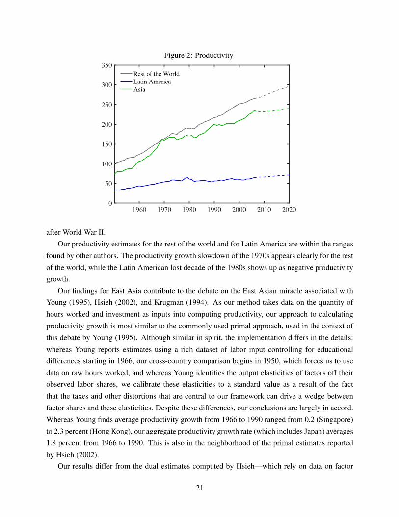
Figure 2: Productivity

1960 1970 1980 1990 2000 2010 20200

50

100

150

200

250

300

350Rest of the WorldLatin AmericaAsia

after World War II.Our productivity estimates for the rest of the world and for Latin America are within the ranges

found by other authors. The productivity growth slowdown of the 1970s appears clearly for the restof the world, while the Latin American lost decade of the 1980s shows up as negative productivitygrowth.

Our findings for East Asia contribute to the debate on the East Asian miracle associated withYoung (1995), Hsieh (2002), and Krugman (1994). As our method takes data on the quantity ofhours worked and investment as inputs into computing productivity, our approach to calculatingproductivity growth is most similar to the commonly used primal approach, used in the context ofthis debate by Young (1995). Although similar in spirit, the implementation differs in the details:whereas Young reports estimates using a rich dataset of labor input controlling for educationaldifferences starting in 1966, our cross-country comparison begins in 1950, which forces us to usedata on raw hours worked, and whereas Young identifies the output elasticities of factors off theirobserved labor shares, we calibrate these elasticities to a standard value as a result of the factthat the taxes and other distortions that are central to our framework can drive a wedge betweenfactor shares and these elasticities. Despite these differences, our conclusions are largely in accord.Whereas Young finds average productivity growth from 1966 to 1990 ranged from 0.2 (Singapore)to 2.3 percent (Hong Kong), our aggregate productivity growth rate (which includes Japan) averages1.8 percent from 1966 to 1990. This is also in the neighborhood of the primal estimates reportedby Hsieh (2002).

Our results differ from the dual estimates computed by Hsieh—which rely on data on factor

21

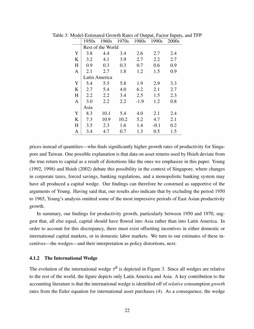
Table 3: Model-Estimated Growth Rates of Output, Factor Inputs, and TFP1950s 1960s 1970s 1980s 1990s 2000sRest of the World

Y 3.8 4.4 3.4 2.6 2.7 2.4K 3.2 4.1 3.9 2.7 2.2 2.7H 0.9 0.3 0.3 0.7 0.6 0.9A 2.1 2.7 1.8 1.2 1.5 0.9

Latin AmericaY 5.4 5.5 5.8 1.9 2.9 3.3K 2.7 5.4 4.0 6.2 2.1 2.7H 2.2 2.2 3.4 2.5 1.5 2.3A 3.0 2.2 2.2 -1.9 1.2 0.8

AsiaY 8.3 10.1 5.4 4.0 2.1 2.4K 7.3 10.9 10.2 5.2 4.7 2.1H 3.5 2.3 1.6 1.4 -0.1 0.2A 3.4 4.7 0.7 1.3 0.5 1.5

prices instead of quantities—who finds significantly higher growth rates of productivity for Singa-pore and Taiwan. One possible explanation is that data on asset returns used by Hsieh deviate fromthe true return to capital as a result of distortions like the ones we emphasize in this paper. Young(1992, 1998) and Hsieh (2002) debate this possibility in the context of Singapore, where changesin corporate taxes, forced savings, banking regulations, and a monopolistic banking system mayhave all produced a capital wedge. Our findings can therefore be construed as supportive of thearguments of Young. Having said that, our results also indicate that by excluding the period 1950to 1965, Young’s analysis omitted some of the most impressive periods of East Asian productivitygrowth.

In summary, our findings for productivity growth, particularly between 1950 and 1970, sug-gest that, all else equal, capital should have flowed into Asia rather than into Latin America. Inorder to account for this discrepancy, there must exist offsetting incentives in either domestic orinternational capital markets, or in domestic labor markets. We turn to our estimates of these in-centives—the wedges—and their interpretation as policy distortions, next.

4.1.2 The International Wedge

The evolution of the international wedge tB is depicted in Figure 3. Since all wedges are relativeto the rest of the world, the figure depicts only Latin America and Asia. A key contribution to theaccounting literature is that the international wedge is identified off of relative consumption growthrates from the Euler equation for international asset purchases (4). As a consequence, the wedge

22

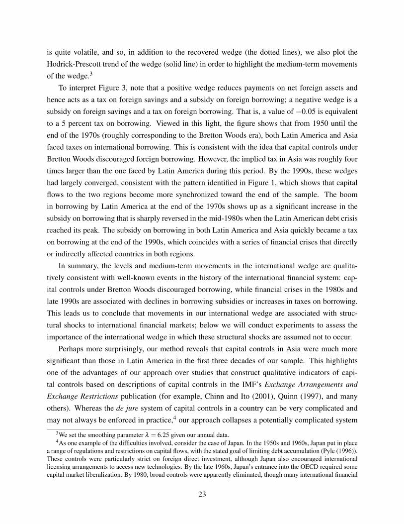
is quite volatile, and so, in addition to the recovered wedge (the dotted lines), we also plot theHodrick-Prescott trend of the wedge (solid line) in order to highlight the medium-term movementsof the wedge.3

To interpret Figure 3, note that a positive wedge reduces payments on net foreign assets andhence acts as a tax on foreign savings and a subsidy on foreign borrowing; a negative wedge is asubsidy on foreign savings and a tax on foreign borrowing. That is, a value of �0.05 is equivalentto a 5 percent tax on borrowing. Viewed in this light, the figure shows that from 1950 until theend of the 1970s (roughly corresponding to the Bretton Woods era), both Latin America and Asiafaced taxes on international borrowing. This is consistent with the idea that capital controls underBretton Woods discouraged foreign borrowing. However, the implied tax in Asia was roughly fourtimes larger than the one faced by Latin America during this period. By the 1990s, these wedgeshad largely converged, consistent with the pattern identified in Figure 1, which shows that capitalflows to the two regions become more synchronized toward the end of the sample. The boomin borrowing by Latin America at the end of the 1970s shows up as a significant increase in thesubsidy on borrowing that is sharply reversed in the mid-1980s when the Latin American debt crisisreached its peak. The subsidy on borrowing in both Latin America and Asia quickly became a taxon borrowing at the end of the 1990s, which coincides with a series of financial crises that directlyor indirectly affected countries in both regions.

In summary, the levels and medium-term movements in the international wedge are qualita-tively consistent with well-known events in the history of the international financial system: cap-ital controls under Bretton Woods discouraged borrowing, while financial crises in the 1980s andlate 1990s are associated with declines in borrowing subsidies or increases in taxes on borrowing.This leads us to conclude that movements in our international wedge are associated with struc-tural shocks to international financial markets; below we will conduct experiments to assess theimportance of the international wedge in which these structural shocks are assumed not to occur.

Perhaps more surprisingly, our method reveals that capital controls in Asia were much moresignificant than those in Latin America in the first three decades of our sample. This highlightsone of the advantages of our approach over studies that construct qualitative indicators of capi-tal controls based on descriptions of capital controls in the IMF’s Exchange Arrangements andExchange Restrictions publication (for example, Chinn and Ito (2001), Quinn (1997), and manyothers). Whereas the de jure system of capital controls in a country can be very complicated andmay not always be enforced in practice,4 our approach collapses a potentially complicated system

3We set the smoothing parameter l = 6.25 given our annual data.4As one example of the difficulties involved, consider the case of Japan. In the 1950s and 1960s, Japan put in place

a range of regulations and restrictions on capital flows, with the stated goal of limiting debt accumulation (Pyle (1996)).These controls were particularly strict on foreign direct investment, although Japan also encouraged internationallicensing arrangements to access new technologies. By the late 1960s, Japan’s entrance into the OECD required somecapital market liberalization. By 1980, broad controls were apparently eliminated, though many international financial

23

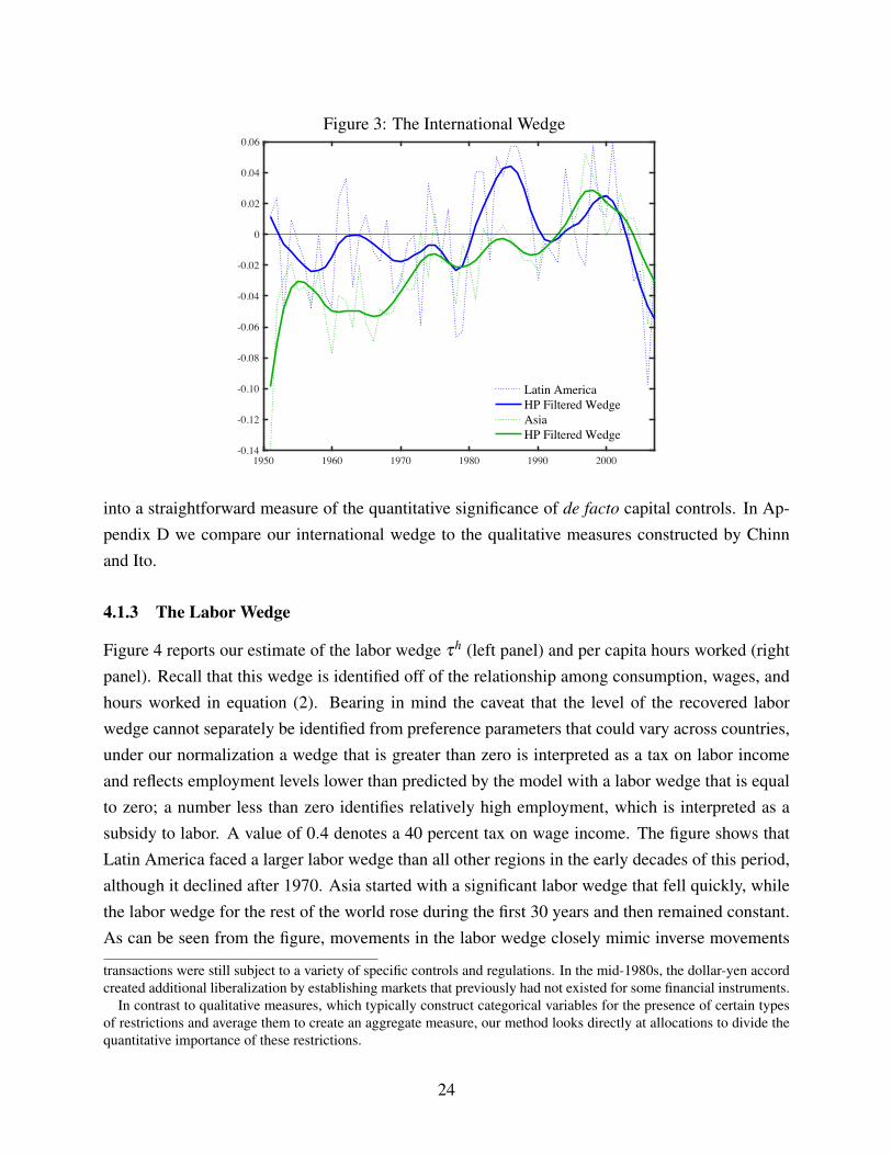
Figure 3: The International Wedge

1950 1960 1970 1980 1990 2000-0.14

-0.12

-0.10

-0.08

-0.06

-0.04

-0.02

0

0.02

0.04

0.06

Latin AmericaHP Filtered WedgeAsiaHP Filtered Wedge

into a straightforward measure of the quantitative significance of de facto capital controls. In Ap-pendix D we compare our international wedge to the qualitative measures constructed by Chinnand Ito.

4.1.3 The Labor Wedge

Figure 4 reports our estimate of the labor wedge th (left panel) and per capita hours worked (rightpanel). Recall that this wedge is identified off of the relationship among consumption, wages, andhours worked in equation (2). Bearing in mind the caveat that the level of the recovered laborwedge cannot separately be identified from preference parameters that could vary across countries,under our normalization a wedge that is greater than zero is interpreted as a tax on labor incomeand reflects employment levels lower than predicted by the model with a labor wedge that is equalto zero; a number less than zero identifies relatively high employment, which is interpreted as asubsidy to labor. A value of 0.4 denotes a 40 percent tax on wage income. The figure shows thatLatin America faced a larger labor wedge than all other regions in the early decades of this period,although it declined after 1970. Asia started with a significant labor wedge that fell quickly, whilethe labor wedge for the rest of the world rose during the first 30 years and then remained constant.As can be seen from the figure, movements in the labor wedge closely mimic inverse movements

transactions were still subject to a variety of specific controls and regulations. In the mid-1980s, the dollar-yen accordcreated additional liberalization by establishing markets that previously had not existed for some financial instruments.

In contrast to qualitative measures, which typically construct categorical variables for the presence of certain typesof restrictions and average them to create an aggregate measure, our method looks directly at allocations to divide thequantitative importance of these restrictions.

24

in hours worked per capita.To interpret the labor wedge, note that it reflects various factors that affect the relationship

between the household’s marginal rate of substitution between consumption and leisure and themarginal product of labor. These may include forces that can be affected by policy, such as laborand consumption taxes (Chari, Kehoe, and McGrattan (2007) and Ohanian, Raffo, and Rogerson(2008)), employment protection laws and other restrictions on hiring or firing workers (Cole andOhanian (2015)), unemployment benefits (Cole and Ohanian (2002)), and limitations on productmarket competition that increase firm monopoly power (Chari, Kehoe, and McGrattan (2007)), aswell as search and matching frictions (Cheremukhin and Restrepo-Echavarria (2014)) that formpart of the “technology” of the economy. As with the international wedge, we show that the laborwedges estimated here often move with changes in taxes and changes in labor market rigidities,leading us to conclude that our estimated labor wedge is capturing structural policy changes thataffect the labor market.

Studies of taxes on labor income and consumption in OECD countries coincide closely withthe rest of the world labor wedge. Prescott (2002) and Ohanian, Raffo, and Rogerson (2008) reportthat in most European countries consumption and labor taxes rose substantially between 1950 andthe mid-1980s and then were roughly stable on average after that (see Figure 22 in Appendix D).This closely mimics the pattern of our labor wedge for the rest of the world that shows an increaseuntil the mid-1970s and little movement thereafter.

In terms of labor market distortions, a number of studies construct measures of these distortionsacross countries. In the most comprehensive study that we know of, Campos and Nugent (2012)construct an index of de jure employment law rigidities for 145 countries between 1950 and 2004.Their approach is similar to that of Botero et al. (2004), who identify labor market rigidities basedon employment, collective bargaining, and social security laws. However, unlike the Botero et al.analysis, the Campos and Nugent data span the full period we analyze.

Our measure of the labor wedge has some patterns that are qualitatively similar to those reportedby Campos and Nugent (2012). Specifically, Campos and Nugent’s measure of aggregated LatinAmerican labor market rigidity shows an increase in rigidity between 1960 and the beginning ofthe 1970s, then a decline until 1985, followed by an increase until 1994, and a larger improvementfrom then on (see plot of the labor market rigidity index in Figure 21 of Appendix D). Our laborwedge follows this pattern. The Campos and Nugent measure of aggregated European labor marketrigidity shows increased rigidity from the 1950s up until the mid-1980s, the same time the rest ofthe world labor wedge is increasing.

For Asia, Campos and Nugent report a relatively modest increase in rigidity throughout the pe-riod (see Figure 21 in Appendix D). Our Asian labor wedge increases after the mid-1990s, whichis qualitatively similar to Campos and Nugent. However, our Asian labor wedge declines con-

25

Figure 4: The Labor Wedge

The Labor Wedge Per Capita Hours Worked

1960 1970 1980 1990 2000-0.1

0

0.1

0.2

0.3

0.4

0.5

0.6

0.7Rest of the WorldLatin AmericaAsia

1960 1970 1980 1990 20000.60

0.70

0.80

0.90

1.00

1.10Rest of the WorldLatin AmericaAsia

siderably before then. This likely reflects factors that are not considered by Campos and Nugent,such as the migration of labor from rural areas, in which labor markets may not be as efficient, tomore urban areas. It may also reflect the changes in education emphasized by Kim (1990), Kim etal. (1980), McGinn (1980), and Ohkawa and Rosovsky (1973) among others. Likewise, the labormarket reforms in Latin America emphasized by Heckman and Pagés (2004), Murillo (2001), andDuryea and Székely (2000) coincide with a decline in the Latin American labor wedge.

In summary, our method recovered quantitatively large movements in labor wedges that coin-cide with important policy changes affecting labor taxes and labor market regulations.

4.1.4 The Capital Wedge

Figure 5 presents our estimates of the capital wedge tK . This wedge is identified off of the Eu-ler equation (3) and thus reflects the difference between returns to investment estimated from themarginal product of capital and the return to savings estimated from the growth rate of consump-tion. Bearing in mind our caveat about the recovered levels of this wedge, under our normalizationa value of 0.05 is equivalent to a 5 percent tax on capital income. As shown in the figure, the restof the world and Latin America have a capital tax (a wedge that is greater than zero), while Asia’scapital wedge deteriorates in the 1950s before falling dramatically between 1960 and 1980. LatinAmerica is estimated as having larger domestic capital market distortions through the mid-1980sduring the debt crisis, with the wedge falling thereafter to levels in between those of Asia and therest of the world.

To assess whether or not these patterns in the capital wedge are consistent with an interpretationof domestic capital market policy distortions, it is useful to compare these results with the IMF’sindex of capital market liberalization (Abiad, Detragiache, and Tressel (2008)). This index wasconstructed from surveyed changes in capital market regulations and restrictions for a numberof countries between 1973 and 2005, including credit controls, interest controls, privatization of

26

banks, entry barriers to banking, the details of banking supervision regimes, and bank reserverequirements. We remove the subindex of changes in international capital market regulations. Theresulting indicator ranges from a value of zero, meaning “fully repressed,” to four, meaning “fullyliberalized.” We find that movements in our estimated capital wedges line up with movements inthe IMF’s index.

According to the IMF index, the four largest Latin American countries—Argentina, Brazil,Chile, and Mexico—liberalized their domestic financial markets between 1973 and 2005, withsome re-regulation occurring in the early to mid-1980s coinciding with the Latin American debtcrisis. Specifically, whereas in 1973 the financial markets of Argentina, Brazil, and Chile wereranked as “fully repressed” and Mexico was ranked as “partially repressed,” these countries imple-mented reforms in the 1970s that included less reliance on interest rate controls, more market-basedsecurities market policies, increased privatization of banks, and increased banking supervision. Thedebt crises of the 1980s saw a temporary reversal of these policy shifts, particularly on interest ratecontrols and credit controls. Following the 1980s, however, Latin America made further progressin the operation of its capital markets, including the reduction of entry barriers, further privatiza-tion of commercial banks, less reliance on interest rate and credit controls, and more market-basedsecurities market policies. By 2005, these countries all had composite rankings of financial mar-kets between fully liberalized and partially liberalized. This general pattern of trend improvementin capital market regulations and restrictions, with a temporary reversal in the 1980s, is consistentwith the estimated capital wedge of Latin America, which trends downward in the 1970s, increasessignificantly during the 1980s, and reverts to its declining trend thereafter.

For Asia, whereas in 1973 the IMF ranked the financial markets of Taiwan as fully repressed,those of Japan as partially repressed, and those of Hong Kong and Singapore as partially liberalized,the 1970s and 1980s saw all of these countries liberalize securities markets and impose fewercontrols on interest rates and credit levels, so that by 2005 all of these countries were ranked asfully liberalized or close to fully liberalized. These patterns dovetail with our estimated capitalwedge for Asia, which shows a trend narrowing over this same period. Appendix D, Figures 23,24, and 25, show the plots of the indices for the different regions.

In summary, as with the labor and international wedges, we conclude that movements in ourestimated wedges are often closely associated with reforms in economic policy. Obviously, it isbeyond the scope of a single paper to provide a full and complete account of the history of laborand capital market policies around the world over half a century of time. However, the summarypresented here documents a close coincidence between movements in labor, domestic capital, andinternational capital wedges and substantive historical policy changes. This leads us to a structuralinterpretation of our wedges as measures of the impact of economic policy distortions. We nextturn to a quantitative assessment of the importance of these distortions in driving capital flows.

27

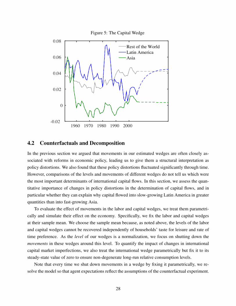
Figure 5: The Capital Wedge

1960 1970 1980 1990 2000-0.02

0

0.02

0.04

0.06

0.08Rest of the WorldLatin AmericaAsia

4.2 Counterfactuals and Decomposition

In the previous section we argued that movements in our estimated wedges are often closely as-sociated with reforms in economic policy, leading us to give them a structural interpretation aspolicy distortions. We also found that these policy distortions fluctuated significantly through time.However, comparisons of the levels and movements of different wedges do not tell us which werethe most important determinants of international capital flows. In this section, we assess the quan-titative importance of changes in policy distortions in the determination of capital flows, and inparticular whether they can explain why capital flowed into slow-growing Latin America in greaterquantities than into fast-growing Asia.

To evaluate the effect of movements in the labor and capital wedges, we treat them parametri-cally and simulate their effect on the economy. Specifically, we fix the labor and capital wedgesat their sample mean. We choose the sample mean because, as noted above, the levels of the laborand capital wedges cannot be recovered independently of households’ taste for leisure and rate oftime preference. As the level of our wedges is a normalization, we focus on shutting down themovements in these wedges around this level. To quantify the impact of changes in internationalcapital market imperfections, we also treat the international wedge parametrically but fix it to itssteady-state value of zero to ensure non-degenerate long-run relative consumption levels.

Note that every time we shut down movements in a wedge by fixing it parametrically, we re-solve the model so that agent expectations reflect the assumptions of the counterfactual experiment.

28

This also implies that the effect of shutting down movements in a wedge will vary according towhether or not movements in other wedges have been shut down or are still operative. As a result,we present two types of results. First, we shut down movements in each individual wedge (oneat a time) and for each evaluate its effect on capital flows keeping all other wedges operative. Weinterpret the results as the effect of removing the corresponding policy distortion while keepingother policy distortions unchanged and refer to these experiments as our counterfactuals. Second,we calculate the relative contribution of each wedge to observed patterns in capital flows as part ofan experiment in which all wedges are shut down. We refer to this series of counterfactuals as ourdecomposition.

4.2.1 Counterfactuals

We begin by shutting down each wedge in isolation. Figure 6 depicts the results of these counter-factual experiments for Latin American and Asian capital flows, as measured by the ratio of netexports to output, respectively, while Figure 7 shows the results for the rest of the world. The fig-ures show the effect of removing each region’s own wedges. This means that, for example, the linelabeled “No Labor Wedge” in the panel for Latin America corresponds to the trajectory followedby net exports in Latin America when the Latin American labor wedge is set parametrically to itsmean value. In the same manner, “No Capital Wedge” and “No International Wedge” correspondto the path followed by net exports when the own-region’s capital wedge is set to its mean valueand its international wedge is set to zero, respectively.

Consider first the effect of shutting down the international wedges. In both Latin America and,especially, Asia, the international wedge was negative at the start of the sample, indicating a taxon borrowing that led both regions to accumulate relatively more foreign assets, or borrow less,than they would have otherwise chosen to do. In the case of Latin America, removing the wedgelowers wealth growth over time and implies correspondingly lower consumption relative to the restof the world during the first three decades, as well as higher hours worked (see Figure 8, whichplots the absolute level of hours, and the level of consumption relative to the data, under eachcounterfactual) and an outflow of capital (compare the black line for the data with the dash-dottedblue lines). Under this counterfactual, the pattern is reversed in the 1980s as Latin America avoidsa debt crisis and relative wealth rises.

In the case of Asia, where the tax on foreign borrowing was larger, removal of the tax leads toan initial increase in consumption and a decline in hours worked, which generates inflows of capitalinto Asia on the order of 5 percent of GDP during the 1950s. However, with wealth no longer risingquickly thereafter, counterfactual consumption soon drops below the level in the data, while hoursworked rise, and for the rest of the sample Asia experiences a large capital outflow. In fact, forthe bulk of the sample, capital outflows from Asia would have been even greater were it not for the

29

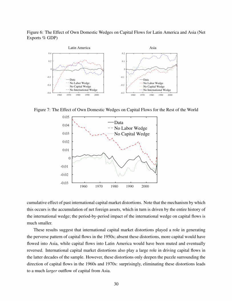
Figure 6: The Effect of Own Domestic Wedges on Capital Flows for Latin America and Asia (NetExports % GDP)

Latin America Asia

1960 1970 1980 1990 2000-0.6

-0.4

-0.2

0

0.2

0.4

DataNo Labor WedgeNo Capital WedgeNo International Wedge

1960 1970 1980 1990 2000-0.3

-0.2

-0.1

0

0.1

0.2

DataNo Labor WedgeNo Capital WedgeNo International Wedge

Figure 7: The Effect of Own Domestic Wedges on Capital Flows for the Rest of the World

1960 1970 1980 1990 2000-0.03

-0.02

-0.01

0

0.01

0.02

0.03

0.04

0.05DataNo Labor WedgeNo Capital Wedge

cumulative effect of past international capital market distortions. Note that the mechanism by whichthis occurs is the accumulation of net foreign assets, which in turn is driven by the entire history ofthe international wedge; the period-by-period impact of the international wedge on capital flows ismuch smaller.

These results suggest that international capital market distortions played a role in generatingthe perverse pattern of capital flows in the 1950s; absent these distortions, more capital would haveflowed into Asia, while capital flows into Latin America would have been muted and eventuallyreversed. International capital market distortions also play a large role in driving capital flows inthe latter decades of the sample. However, these distortions only deepen the puzzle surrounding thedirection of capital flows in the 1960s and 1970s: surprisingly, eliminating these distortions leadsto a much larger outflow of capital from Asia.

30

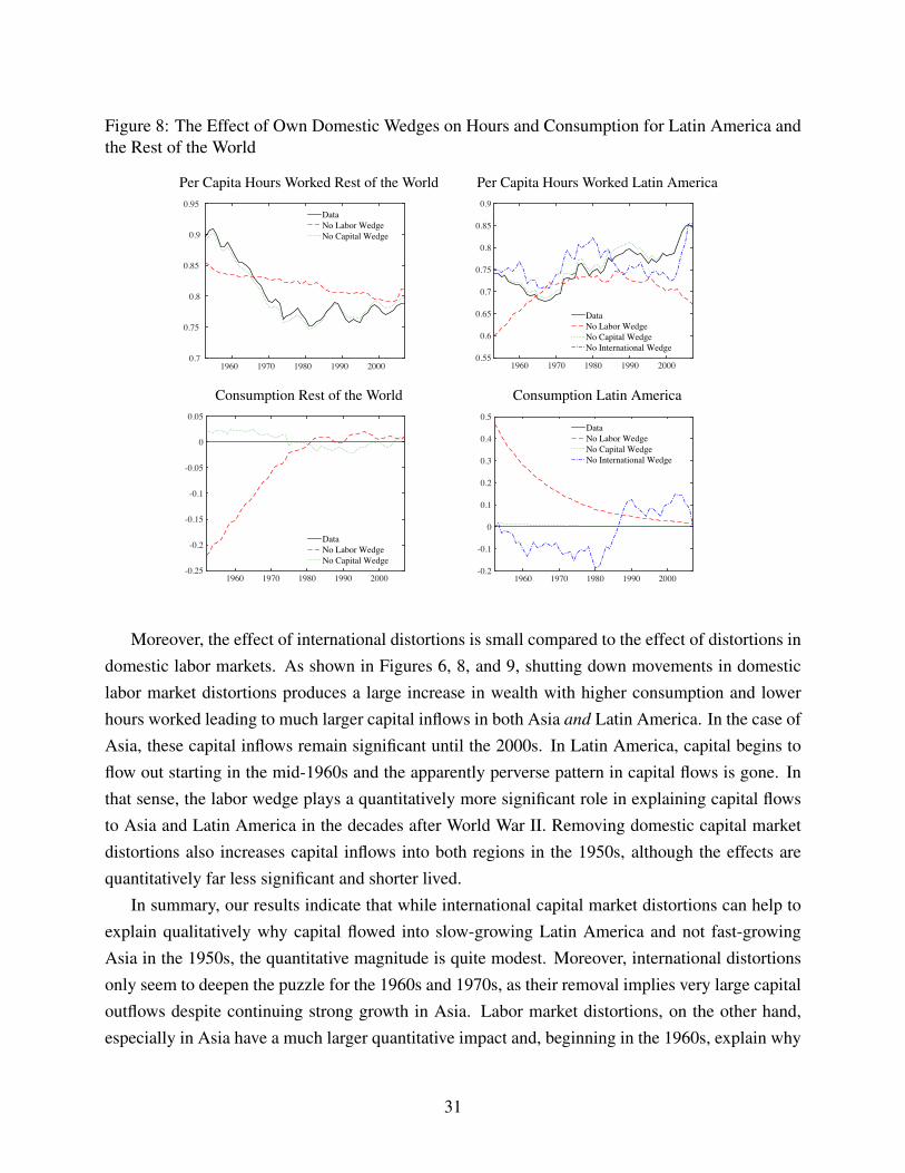
Figure 8: The Effect of Own Domestic Wedges on Hours and Consumption for Latin America andthe Rest of the World

Per Capita Hours Worked Rest of the World Per Capita Hours Worked Latin America

1960 1970 1980 1990 20000.7

0.75

0.8

0.85

0.9

0.95DataNo Labor WedgeNo Capital Wedge

1960 1970 1980 1990 20000.55

0.6

0.65

0.7

0.75

0.8

0.85

0.9

DataNo Labor WedgeNo Capital WedgeNo International Wedge

Consumption Rest of the World Consumption Latin America

1960 1970 1980 1990 2000-0.25

-0.2

-0.15

-0.1

-0.05

0

0.05

DataNo Labor WedgeNo Capital Wedge

1960 1970 1980 1990 2000-0.2

-0.1

0

0.1

0.2

0.3

0.4

0.5DataNo Labor WedgeNo Capital WedgeNo International Wedge

Moreover, the effect of international distortions is small compared to the effect of distortions indomestic labor markets. As shown in Figures 6, 8, and 9, shutting down movements in domesticlabor market distortions produces a large increase in wealth with higher consumption and lowerhours worked leading to much larger capital inflows in both Asia and Latin America. In the case ofAsia, these capital inflows remain significant until the 2000s. In Latin America, capital begins toflow out starting in the mid-1960s and the apparently perverse pattern in capital flows is gone. Inthat sense, the labor wedge plays a quantitatively more significant role in explaining capital flowsto Asia and Latin America in the decades after World War II. Removing domestic capital marketdistortions also increases capital inflows into both regions in the 1950s, although the effects arequantitatively far less significant and shorter lived.

In summary, our results indicate that while international capital market distortions can help toexplain qualitatively why capital flowed into slow-growing Latin America and not fast-growingAsia in the 1950s, the quantitative magnitude is quite modest. Moreover, international distortionsonly seem to deepen the puzzle for the 1960s and 1970s, as their removal implies very large capitaloutflows despite continuing strong growth in Asia. Labor market distortions, on the other hand,especially in Asia have a much larger quantitative impact and, beginning in the 1960s, explain why

31

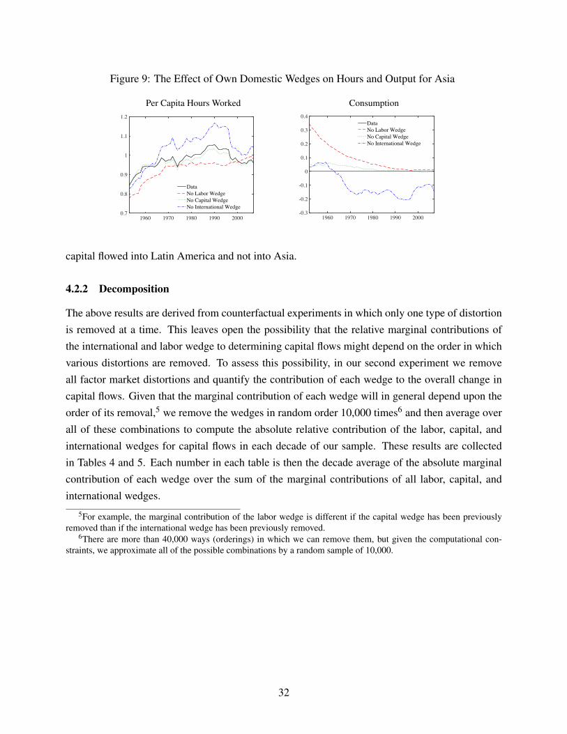
Figure 9: The Effect of Own Domestic Wedges on Hours and Output for Asia

Per Capita Hours Worked Consumption

1960 1970 1980 1990 20000.7

0.8

0.9

1

1.1

1.2

DataNo Labor WedgeNo Capital WedgeNo International Wedge

1960 1970 1980 1990 2000-0.3

-0.2

-0.1

0

0.1

0.2

0.3

0.4DataNo Labor WedgeNo Capital WedgeNo International Wedge

capital flowed into Latin America and not into Asia.

4.2.2 Decomposition

The above results are derived from counterfactual experiments in which only one type of distortionis removed at a time. This leaves open the possibility that the relative marginal contributions ofthe international and labor wedge to determining capital flows might depend on the order in whichvarious distortions are removed. To assess this possibility, in our second experiment we removeall factor market distortions and quantify the contribution of each wedge to the overall change incapital flows. Given that the marginal contribution of each wedge will in general depend upon theorder of its removal,5 we remove the wedges in random order 10,000 times6 and then average overall of these combinations to compute the absolute relative contribution of the labor, capital, andinternational wedges for capital flows in each decade of our sample. These results are collectedin Tables 4 and 5. Each number in each table is then the decade average of the absolute marginalcontribution of each wedge over the sum of the marginal contributions of all labor, capital, andinternational wedges.

5For example, the marginal contribution of the labor wedge is different if the capital wedge has been previouslyremoved than if the international wedge has been previously removed.

6There are more than 40,000 ways (orderings) in which we can remove them, but given the computational con-straints, we approximate all of the possible combinations by a random sample of 10,000.

32

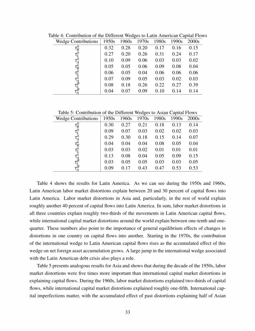
Table 4: Contribution of the Different Wedges to Latin American Capital FlowsWedge Contributions 1950s 1960s 1970s 1980s 1990s 2000s

thR 0.32 0.28 0.20 0.17 0.16 0.15

thL 0.27 0.20 0.26 0.31 0.24 0.17

thA 0.10 0.09 0.06 0.03 0.03 0.02

tkR 0.05 0.05 0.06 0.09 0.08 0.04

tkL 0.06 0.05 0.04 0.06 0.06 0.06

tkA 0.07 0.09 0.05 0.03 0.02 0.03

tBL 0.08 0.18 0.26 0.22 0.27 0.39

tBA 0.04 0.07 0.09 0.10 0.14 0.14

Table 5: Contribution of the Different Wedges to Asian Capital FlowsWedge Contributions 1950s 1960s 1970s 1980s 1990s 2000s

thR 0.30 0.27 0.21 0.18 0.13 0.14

thL 0.09 0.07 0.03 0.02 0.02 0.03

thA 0.29 0.30 0.18 0.15 0.14 0.07

tkR 0.04 0.04 0.04 0.08 0.05 0.04

tkL 0.03 0.03 0.02 0.01 0.01 0.01

tkA 0.13 0.08 0.04 0.05 0.09 0.15

tBL 0.03 0.05 0.05 0.03 0.03 0.05

tBA 0.09 0.17 0.43 0.47 0.53 0.53

Table 4 shows the results for Latin America. As we can see during the 1950s and 1960s,Latin American labor market distortions explain between 20 and 30 percent of capital flows intoLatin America. Labor market distortions in Asia and, particularly, in the rest of world explainroughly another 40 percent of capital flows into Latin America. In sum, labor market distortions inall three countries explain roughly two-thirds of the movements in Latin American capital flows,while international capital market distortions around the world explain between one-tenth and one-quarter. These numbers also point to the importance of general equilibrium effects of changes indistortions in one country on capital flows into another. Starting in the 1970s, the contributionof the international wedge to Latin American capital flows rises as the accumulated effect of thiswedge on net foreign asset accumulation grows. A large jump in the international wedge associatedwith the Latin American debt crisis also plays a role.

Table 5 presents analogous results for Asia and shows that during the decade of the 1950s, labormarket distortions were five times more important than international capital market distortions inexplaining capital flows. During the 1960s, labor market distortions explained two-thirds of capitalflows, while international capital market distortions explained roughly one-fifth. International cap-ital imperfections matter, with the accumulated effect of past distortions explaining half of Asian

33

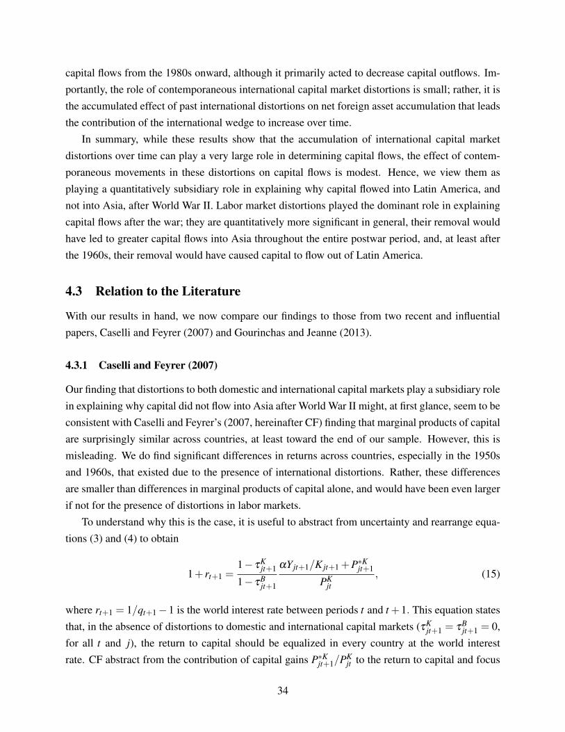
capital flows from the 1980s onward, although it primarily acted to decrease capital outflows. Im-portantly, the role of contemporaneous international capital market distortions is small; rather, it isthe accumulated effect of past international distortions on net foreign asset accumulation that leadsthe contribution of the international wedge to increase over time.

In summary, while these results show that the accumulation of international capital marketdistortions over time can play a very large role in determining capital flows, the effect of contem-poraneous movements in these distortions on capital flows is modest. Hence, we view them asplaying a quantitatively subsidiary role in explaining why capital flowed into Latin America, andnot into Asia, after World War II. Labor market distortions played the dominant role in explainingcapital flows after the war; they are quantitatively more significant in general, their removal wouldhave led to greater capital flows into Asia throughout the entire postwar period, and, at least afterthe 1960s, their removal would have caused capital to flow out of Latin America.

4.3 Relation to the Literature

With our results in hand, we now compare our findings to those from two recent and influentialpapers, Caselli and Feyrer (2007) and Gourinchas and Jeanne (2013).

4.3.1 Caselli and Feyrer (2007)

Our finding that distortions to both domestic and international capital markets play a subsidiary rolein explaining why capital did not flow into Asia after World War II might, at first glance, seem to beconsistent with Caselli and Feyrer’s (2007, hereinafter CF) finding that marginal products of capitalare surprisingly similar across countries, at least toward the end of our sample. However, this ismisleading. We do find significant differences in returns across countries, especially in the 1950sand 1960s, that existed due to the presence of international distortions. Rather, these differencesare smaller than differences in marginal products of capital alone, and would have been even largerif not for the presence of distortions in labor markets.

To understand why this is the case, it is useful to abstract from uncertainty and rearrange equa-tions (3) and (4) to obtain

1+ rt+1 =1� tK

jt+1

1� tBjt+1

aYjt+1/Kjt+1 +P⇤Kjt+1

PKjt

, (15)

where rt+1 = 1/qt+1 �1 is the world interest rate between periods t and t +1. This equation statesthat, in the absence of distortions to domestic and international capital markets (tK

jt+1 = tBjt+1 = 0,

for all t and j), the return to capital should be equalized in every country at the world interestrate. CF abstract from the contribution of capital gains P⇤K

jt+1/PKjt to the return to capital and focus

34

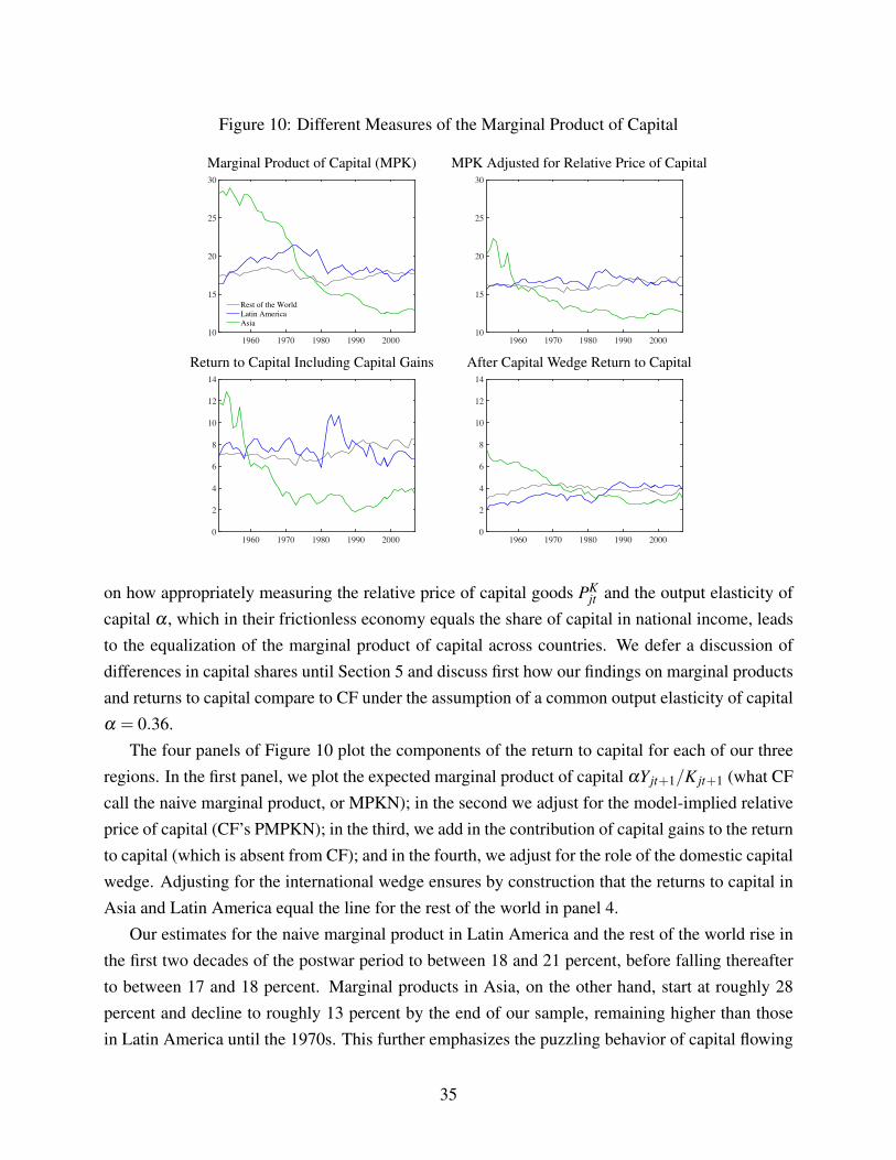
Figure 10: Different Measures of the Marginal Product of Capital

Marginal Product of Capital (MPK) MPK Adjusted for Relative Price of Capital

1960 1970 1980 1990 200010

15

20

25

30

Rest of the WorldLatin AmericaAsia

1960 1970 1980 1990 200010

15

20

25

30

Return to Capital Including Capital Gains After Capital Wedge Return to Capital

1960 1970 1980 1990 20000

2

4

6

8

10

12

14

1960 1970 1980 1990 20000

2

4

6

8

10

12

14

on how appropriately measuring the relative price of capital goods PKjt and the output elasticity of

capital a , which in their frictionless economy equals the share of capital in national income, leadsto the equalization of the marginal product of capital across countries. We defer a discussion ofdifferences in capital shares until Section 5 and discuss first how our findings on marginal productsand returns to capital compare to CF under the assumption of a common output elasticity of capitala = 0.36.

The four panels of Figure 10 plot the components of the return to capital for each of our threeregions. In the first panel, we plot the expected marginal product of capital aYjt+1/Kjt+1 (what CFcall the naive marginal product, or MPKN); in the second we adjust for the model-implied relativeprice of capital (CF’s PMPKN); in the third, we add in the contribution of capital gains to the returnto capital (which is absent from CF); and in the fourth, we adjust for the role of the domestic capitalwedge. Adjusting for the international wedge ensures by construction that the returns to capital inAsia and Latin America equal the line for the rest of the world in panel 4.

Our estimates for the naive marginal product in Latin America and the rest of the world rise inthe first two decades of the postwar period to between 18 and 21 percent, before falling thereafterto between 17 and 18 percent. Marginal products in Asia, on the other hand, start at roughly 28percent and decline to roughly 13 percent by the end of our sample, remaining higher than thosein Latin America until the 1970s. This further emphasizes the puzzling behavior of capital flowing

35

into Latin America instead of Asia immediately after the war. These naive marginal products forAsia and the rest of the world are higher at the end of the sample than those from CF (Japan andthe United States are at 9 and 12 percent, respectively) but are similar for Latin America (Mexico’sis 22 percent and Colombia’s is 28 percent, for example). After adjusting for the relative price ofcapital, returns in Latin America and the rest of the world converge dramatically, even more so thanin CF’s estimates, albeit to somewhat higher levels. Asian returns remain higher than those in LatinAmerica for only the first decade.

Including capital gains (which includes the effect of depreciation and is shown in panel 3)lowers returns in Latin America and the rest of the world to around 8 percent and in Asia to around4 percent by the end of the sample. Accounting for the capital wedge (panel 4) lowers returns atthe start of the sample and compresses them toward the end, with all three countries between 3 and4 percent. The international wedge, by construction and given our normalization, causes all returnsto converge to that of the rest of the world in the fourth panel.

Panel 4 shows that, if there were no international wedge, during the 1950s, an investor in therest of the world would have made an additional 4 percent return investing in Asia and a negativereturn of roughly 1 percent investing in Latin America. In that sense, there were bad investmentsin Latin America and missed opportunities in Asia. Returns in Asia remain higher than those inLatin America until the 1980s, although both returns are lower than in the rest of the world after the1970s. In this sense, the international wedge helps to explain the puzzling absence of capital inflowsinto Asia in the 1950s and 1960s, and the puzzling inflows of capital into Latin America up untilthe mid-1980s. Interestingly, absent both the international and capital wedges, the investor wouldhave made 1 percent (Latin America) to 3 percent (Asia) higher returns from investing abroad ineither region in the 1950s.

This is the main difference between our results and those of CF: we find significant differencesin returns to capital across countries—especially in the 1950s and 1960s—that persist only due tointernational capital market distortions. However, our results are closer in spirit to CF in that wefind that differences in returns would have been even larger still had it not been for distortions inlabor markets. To see this most clearly, consider Asia, which, according to our results for 1950,had a marginal product of capital (panel 1) that is 11 percentage points higher, and a return tocapital after capital gains and domestic capital market distortions (panel 4) that is 4.5 percentagepoints higher, than in the rest of the world. These differences are large but were entirely erased by1980. However, the differences in 1950 and the declines thereafter would have been much largerstill were it not for high and declining labor market distortions in Asia. To see this, note that hoursworked per person in Asia were roughly one-third lower in 1950 than they were in 1980. Had hoursworked per person in 1950 been closer to their 1980 levels, the marginal product in Asia would havebeen almost 17 percentage points higher than in the rest of the world. Similarly, had labor market

36

distortions not been unwound over the decades after 1950, the marginal product of capital wouldhave fallen to roughly 3 percentage points below that in the rest of the world by 1980, instead ofbeing within a percentage point. We therefore conclude that labor market distortions played a moresignificant role in driving differences in returns and the incentives to reallocate capital.

So far, we have not considered CF’s argument that capital shares as typically constructed inthe data may overestimate the true share of reproducible capital due to the inclusion of returns tonon-reproducible factors such as land and natural resources. We have three reasons for this. First,measured capital shares will not correctly identify the output elasticity of capital if capital mar-ket distortions are not recorded as payments to capital, even in the absence of non-reproduciblecapital returns. Thus, we prefer to calibrate the output elasticity of capital to a common value. Sec-ond, measured capital shares need not accurately reflect after-tax and subsidy payments to capital.Third, CF’s adjustments to capital shares often result in returns to capital that seem implausiblylow (see also Ohanian and Wright (2008)). Specifically, under CF’s assumption of a 6 percentdepreciation rate, their implied return to capital is non-positive in 17 out of 52 countries. Allowingfor an additional decline in capital prices of between 3 and 4 percent due to technological progress(Greenwood and Yorukoglu (1997) find that equipment prices fell 3.3 percent per year prior to 1974and 4 percent thereafter) results in negative returns to capital for all but 8 (if we use 3 percent) or7 (if we use 4 percent) countries in their sample. Note that these returns are negative; they are cer-tainly less than the return on a real government bond. Nonetheless, in the robustness section below,we report results from experiments in which we calibrate capital shares to the levels estimated forreproducible capital by CF and show that, when the model is re-estimated under these assumptions,our results are largely unchanged.

4.3.2 Gourinchas and Jeanne (2013)

Our finding that the international wedge plays only a small role in determining capital flows standsin stark contrast to the finding of Gourinchas and Jeanne (2013, hereinafter GJ) that this wedge (GJcall it a savings wedge) plays the dominant role in accounting for observed capital flows. Thereare several complementary reasons for this. One of the most significant reasons results from GJ’sdifferent definition of the capital wedge. Specifically, whereas we define our capital wedge as thedifference between a household’s marginal rate of substitution and domestic capital returns, GJdefine their capital wedge as the difference between domestic capital returns and the world interestrate. That is, their capital wedge is equivalent to the ratio of our capital wedge to our internationalwedge. More importantly, their experiments varying their savings wedge while keeping their capitalwedge constant are equivalent to varying both our international and capital wedges simultaneously,which produces a compounded effect. Combined with an absence of transitional dynamics in theirmodel, this results in much larger effects of the savings wedge on capital flows.

37

The other major difference comes from their treatment of the labor supply. This has two di-mensions. First, empirically, GJ measure labor input as the working-age population. This meansthat in their measurement of productivity growth, GJ attribute any variation in hours per person tochanges in productivity. This also leaves no role for the labor wedge in their analysis. Second,in their theory, the labor supply is held constant, which is strongly at variance with the very largechanges in hours per worker documented here. This matters because, when they vary their sav-ings wedge, their measure of productivity (which includes any implicit effect from a variable laborsupply) is held constant. When labor supply is endogenous, changes in the savings wedge wouldimply changes in wealth that lead to changes in labor supply that would change their measure ofproductivity. Specifically, the positive savings wedges (which act as taxes on borrowing) necessaryto explain why capital did not flow into Asia in their analysis, taking as given their measure ofproductivity growth for Asia, would in fact lead to declines in hours worked per person and anendogenous decline in their measure of productivity growth. This amplifies the effect of changesin the savings wedge in their framework, relative to ours.

5 Robustness and Extensions

In this section, we briefly discuss the robustness of our findings. We consider robustness withrespect to changes in the specification of our benchmark model and the robustness of our structuralinterpretation of the wedges as reflecting factor market distortions. We also consider how ourresults relate to some other studies of international capital flows that have emphasized different andcomplementary moments of the data. A more detailed discussion of these issues is available inAppendix E.

5.1 Parameter Values

Above we wrote down a benchmark model against which the data could be compared, with aview toward identifying wedges between what the model predicts and what the data show. As isconventional, and for concreteness, we interpreted these wedges as taxes and subsidies that affectthe marginal optimality conditions of firms and households. In discussing our results, we comparedour estimated wedges with both qualitative and quantitative indicators of taxes and factor marketdistortions and argued that the results were similar. That is, the interpretation of these wedges asa combination of taxes and subsidies and non-tax distortions was reasonable. Nonetheless, anydifferences between our benchmark model and the “true model” of the data-generating process willalso show up as wedges. One possible cause of misspecification arises from specific functionalforms and parameter choices. In this subsection, we illustrate how alternative assumptions about

38

parameter values affect the identified wedges and the resulting analysis.A number of parameter choices have precisely no effect on our results, as they serve only to

scale up or down the estimates of the wedges, and our experiments set wedges to their mean levels.These include the discount factor b , which, as long as it is constant across countries, only affectsthe steady-state level of the capital wedge in each country. It also includes the preference for leisureparameter j, which is indistinguishable from the steady-state labor wedge and could be allowedto vary across countries. Other parameters appear to have small effects: for example, allowingthe intertemporal elasticity of substitution to depart from 1 changes the levels of the wedges—thelower the elasticity, the more wedges must vary to explain changes in behavior. But this departureseems to have only small effects on our experiments—a low elasticity also dampens the response tosetting these wedges constant. Likewise, increasing the Frisch elasticity of labor supply dampensmovements in the recovered wedges, but correspondingly increases the response from shuttingdown these same movements.

Of the remaining parameters, one that might have a significant effect on the model is the levelof the capital adjustment cost n , which is known to be a very important determinant of capitalflows in open economy macroeconomic models (see, for example, Baxter and Crucini (1993) for adiscussion). In our benchmark, we set this to generate an elasticity of the price of capital to the ratioof investment to capital of 1/2, which is the upper bound of what Bernanke, Gertler, and Gilchrist(1999) consider plausible, but arguably better describes emerging market countries. In the onlineappendix, we also present results using Bernanke, Gertler, and Gilchrist’s preferred value of 1/4 forthe United States and show that it leads to very similar results.

Another parameter that has been a focal point of the literature is the output elasticity of capital,which in an undistorted economy equals the capital share. As noted above, CF argue that the truecapital share should exclude payments to non-reproducible factors of production, such as land, andprovide an adjustment that shows significant differences in these shares across countries. Changingthe output elasticity of capital a not only will directly affect the labor and capital wedges, as canbe seen in equations (13) and (14), but also will affect the entire equilibrium of the model. Toassess whether this makes a significant difference to our results, we calculated our wedges after re-estimating the model with output elasticities of capital calibrated to be different across regions andequal to the income-weighted share of the estimates of CF. Whereas in the baseline we imposed a =

0.36 for all countries, this results in output elasticities of capital of aASIA = 0.23, aLATAM = 0.26,and aROW = 0.18. The resulting estimates of the capital and labor wedges using heterogeneouscapital shares look like scaled versions of those computed in our benchmark. This is perhaps notsurprising: ignoring the effect of the equilibrium of the model, increasing/decreasing a servesmostly to decrease/increase the estimated capital wedge each period. Given that our experimentsset the capital wedge equal to its sample mean, the resulting outcomes of our experiments also turn

39

out to be both qualitatively and quantitatively similar to those for our benchmark.A recent literature has pointed to movements in the capital share in the United States and some

other countries over time and has argued that this is evidence that the aggregate production functionis not well approximated by a Cobb-Douglas production function. While this is one possible inter-pretation of varying factor shares, another possibility consistent with the mechanism of our paper isthat changes in factor market distortions are responsible for the changing levels of the factor share.This would be the case if these factor market distortions are not priced or otherwise measured ascompensation for the relevant factor of production and would imply that measured factor sharesdo not identify the relevant parameter of the Cobb-Douglas production function nor indicate anydeparture from Cobb-Douglas. Differences in the levels of factor market frictions across countriescould also explain recorded differences in the levels of capital shares across countries, and not justtime-series variation in factor shares. Given these possibilities, we do not further explore them.

Lastly, we imposed the assumption that our wedges were uncorrelated across countries. Thiswas for simplicity, as it drastically reduced the number of parameters to be estimated on less than 60years of annual data; instead of 34 parameters, a vector autoregressive structure for our 17 wedgeswould require the estimation of 172 = 289 autoregressive coefficients and a further 153 parame-ters in the covariance matrix. Nonetheless, correlation among the labor, capital, and internationalwedges could matter for the interpretation of our experiments, in which movement in a given wedgeis shut down. To examine the potential for this issue, we looked at the empirical relationship amongour recovered wedges. Economically, the correlations between the wedges are typically small, with66 percent of the parameters in the correlation matrix being less than 0.5 in absolute value. Thelargest correlations tend to be associated with the cross-country relationships between populationand productivity.

As our experiments concerned shutting down the international, capital, and labor wedges, witha focus on those wedges specific to Latin America and Asia, we are mostly concerned with interac-tions among these wedges and all other wedges. One way to assess this is to compute the principalcomponents of the covariance matrix of the wedges.

The first two principal components explain almost 92 percent of the variation in the data. Ofthese, the first principal component, which explains roughly 73 percent of the variation in the data,loads primarily on the population and productivity wedges of Asia and Latin America as well ason Asian government spending. The second principal component, which explains 19 percent of thevariation in the data, loads primarily on the productivity of Asia and the capital wedge for the restof the world and Asia. While one might tell an economic story in which these are related, we thinkit more likely reflects a spurious relationship in the short sample. As a consequence, we concludethat the correlation among the wedges that we focus on is small and not an important factor drivingour results.

40

5.2 Alternative Structural Interpretations of Wedges

In this subsection, we briefly discuss some examples of alternative models of, and explanations for,observed patterns in international capital flows. In each case, we briefly sketch how the alternativeexplanation would manifest as patterns in the wedges recovered from our analysis. Further detailsare provided in Appendix E.

5.2.1 Multiple Goods and Transport Costs

Our benchmark model featured one tradable consumption good for the world and one non-tradableinvestment good in each country. This means that the terms of trade are constant and that anymovements in the terms of trade in the data will be attributed to our wedges. To see how thisaffects our wedges, consider the two-country model of Backus, Kehoe, and Kydland (1994) inwhich a domestically produced tradable good is combined with a foreign-produced tradable goodto produce a non-traded domestic good that is both consumed and invested. The assumption of twocountries simplifies the analysis by making relative price calculations obvious.

It is straightforward to show (see Appendix E) that if data generated by this model were con-fronted with the capital flow accounting procedure above, the resulting wedges in our benchmarkmodel would be correlated with the level and change in a country’s terms of trade. Specifically,when the price of a country’s export good falls relative to the price of the good it imports, so that itsterms of trade deteriorate, both the labor and capital wedges get larger. This is intuitive: for a givennominal wage, an increase in import prices reduces the real returns to suppliers of labor and capitalwhile leaving the real costs to the firm unchanged. The international wedge, on the other hand, willin general respond to the growth rate of the terms of trade as relative inflation across countries, andhence also relative real returns, move in opposite directions. Inspection of the wedges recoveredfrom the data shows at best modest evidence for these patterns, suggesting that this explanationdoes not play a major role in explaining observed capital flows.

Relatedly, Obstfeld and Rogoff (2001), Fitzgerald (2012), and others have argued that transportcosts in international trade can drive movements in relative prices that provide a qualitative, andpossibly also a quantitative, explanation of some observed patterns in capital flows. Regarding thelevel of capital flows, intuitively, in a finite horizon economy, a country that is a borrower (netimporter) today will be a net exporter at some point in the future when these debts are repaid. Ifthis causes a country to shift from importing a given set of goods (at a high price due to paymentof transport costs) to exporting them (at a lower price due to foreigners paying these same costs),there will be domestic deflation and a high real cost of borrowing from abroad. Likewise, a countrythat saves will tend to receive lower real returns. Thus, the level of capital flows may be reduced.Reyes-Heroles (2016), Alessandria and Choi (2015), and Eaton, Kortum, and Neiman (2016) all

41

find that trade costs play significant (but quantitatively varying) roles in explaining the level ofcapital flows in the context of their own models. However, it is not clear that this mechanism playsa quantitatively significant role in explaining relative levels of capital flows to Latin America andAsia in practice. Further discussion is provided in Appendix E.

5.2.2 Financial Frictions

Our finding of a dominant role for labor market distortions may be viewed as surprising when setagainst the large literature that has examined the role of various financial frictions in determiningcapital flows. In the case of Latin America in particular, which experienced a sovereign debt crisisin the middle of our sample, one might expect frictions resulting from the enforcement of contractsto play a significant role. In this subsection, we briefly review the implications of the class oflimited commitment models for our results.

Consider a limited commitment model of international financial frictions along the lines ofKehoe and Perri (2002; see also Wright (2001)). In Appendix E, we show that the shadow cost ofbinding enforcement constraints shows up directly in our international wedge. In a limited commit-ment model, regardless of whether or not capital flows are motivated by consumption smoothing,capital scarcity, or a desire to shift consumption through time (that is, tilt the consumption profile),the model predicts that the participation constraint should never bind when net exports are negative.Intuitively, this is because a country is never tempted to refuse a positive inflow of resources fromthe rest of the world. As we can see in Figure 3 above, the upward movement in the internationalwedges in Asia and Latin America in the 1980s coincides with the switch from negative to positivenet exports for both regions, providing support for this model in the 1980s (see also Restrepo-Echavarria (2018)). However, this mechanism appears to play no role in explaining capital flowsin the 1950s and 1960s, which is the focus of our analysis. Moreover, limited commitment modelsimply an international wedge that is highly correlated with the capital wedge, and these modelsgenerate no labor wedge at all. We find no support for these predictions in the data.

5.3 Public Capital Flows and Ricardian Equivalence

Some authors, such as Aguiar and Amador (2016) and Alfaro, Kalemli-Ozcan, and Volosovych(2014), have argued that public capital flows—borrowing and saving by emerging market countrygovernments—are the key component in explaining capital flows beginning in the 1970s. It is alsopossible that similar forces were also relevant in the early decades that are our focus, although datalimitations prevent an extension of their analysis back to 1950. Implicitly, of course, this requiresthat there must be a significant departure from Ricardian equivalence that prevents private capitalflows (that is, flows to the private sector of these economies) from offsetting these public flows. We

42

are quite open to this possibility and note that plausible reasons for the departure from Ricardianequivalence have testable implications that our wedges approach is well designed to examine.

Specifically, one leading hypothesis must be that the capital controls that were introduced underthe Bretton-Woods system prevented the private sector from accessing international capital marketsto offset the effect of public capital flows. But this implies that private consumption should departfrom the levels implied by the Euler equation for bonds, which would show up as an internationalwedge in our framework. The fact that we find that the international wedge has a relatively smallimpact on capital flows is evidence against this departure from Ricardian equivalence being impor-tant in explaining capital flows. Other possibilities, such as myopia on the behalf of consumers,would also show up as both an international and a capital wedge.

These possibilities should not necessarily be taken as evidence against the claim that public cap-ital flows drive national capital flows during this period. Instead, it might simply imply a differentdeparture from Ricardian equivalence. We view our approach as complementary to this argument inthat it provides evidence of what these departures from Ricardian equivalence might be and believeit will be a fruitful avenue for future research.

6 Conclusion

Between 1950 and 1990, Asia grew much faster than Latin America but received fewer capitalinflows from abroad. This is surprising because, all else equal, rapidly growing countries shouldgenerate higher capital returns and thus should receive more capital than slow-growing countries.Some studies implicitly adopt the “all else equal” aspect of this argument and analyze capital flowpatterns by focusing on imperfections and inefficiencies of international capital markets that eitherdepress the incentives, or limit the opportunities, to move capital to fast-growing regions. In thispaper, we removed the “all else equal” assumption and explored the role of domestic labor marketdistortions in influencing the return to capital and the incentives for capital flows.

Specifically, we developed a capital flow accounting framework that can be thought of as a formof open economy business cycle accounting. We then applied this to a novel dataset of output,consumption, investment, hours worked, and international capital flows for Asia, Latin America,and the rest of the world from 1950 to 2007. We used this framework and data to measure impliedlabor market and both domestic and international capital market distortions and to quantify theimpact of these factors on international capital flows.

We found that labor market distortions, and their removal over time, play the dominant role inexplaining both why Asia grew relatively fast as well as why it received little in the way of capitalinflows. Perhaps surprisingly, in light of the preceding literature, the impact of international anddomestic capital market distortions was not quantitatively important in deterring capital flows into

43

Asia after the 1950s, and in fact acted to decrease capital outflows from Asia. Latin Americancapital flows were also primarily driven by the Latin American labor wedge. International capitalmarket distortions had much larger effects on Latin American capital flows during and after theLatin American debt crisis of the 1980s.

These findings have both positive and normative implications. On the positive side, the resultsindicate that there is no presumption that rapidly growing countries should receive disproportion-ately high capital flows, as domestic labor and capital market distortions can sufficiently depressthe incentives to move capital to these countries. On the normative side, our findings also suggestthat the welfare effects of reforming domestic institutions can be much larger than often assumed,as changes in domestic distortions can have large direct and indirect effects on world allocations.

44

References

1. Abiad, Abdul, Enrica Detragiache and Thierry Tressel. 2008. “A New Database of FinancialReforms.” IMF Working Paper WP/08/266, December.

2. Aguiar, Mark and Manuel Amador. 2016. “Fiscal Policy in Debt Constrained Economies.”Journal of Economic Theory, 161: 37-75.

3. Aguiar, Mark, and Gita Gopinath. 2006. “Defaultable Debt, Interest Rates and the CurrentAccount.” Journal of International Economics, 69(1): 64-83.

4. Alessandria, George and Horag Choi. 2015. “The Dynamics of the Trade Balance and theReal Exchange Rate: The J Curve and Trade Costs?” Unpublished manuscript.

5. Alfaro, Laura, Sebnem Kalemli-Ozcan and Vadym Volosovych. 2008. “Why Doesn’t CapitalFlow from Rich to Poor Countries? An Empirical Investigation.” Review of Economics andStatistics, 90(2), 347-68.

6. Alfaro, Laura, Sebnem Kalemli-Ozcan and Vadym Volosovych. 2014. “Sovereigns, Up-stream Capital Flows, and Global Imbalances.” Journal of the European Economic Associa-tion, 12(5): 1240-84.

7. An, Sungbae and Frank Schorfheide. 2007. “Bayesian Analysis of DSGE Models.” Econo-metric Reviews, 26(2-4): 113-72.

8. Arellano, Cristina. 2008. “Default Risk and Income Fluctuations in Emerging Economies.”American Economic Review, 98(3): 690-712.

9. Atkeson, Andrew. 1991. “International Lending with Moral Hazard and Risk of Repudia-tion.” Econometrica, 59(4): 1069-89, July.

10. Backus, David K., Patrick J Kehoe, and Finn E. Kydland. 1994. “Dynamics of the TradeBalance and the Terms of Trade: The J-Curve?” American Economic Review, 84(1): 84-103.

11. Bai, Yan and Jing Zhang. 2010. “Solving the Feldstein-Horioka Puzzle with Financial Fric-tions.” Econometrica, 78(2): 603-32.

12. Bayoumi, Tamim and Andrew K. Rose. 1993. “Domestic Savings and Intra-National CapitalFlows.” European Economic Review, 37(6): 1197-202.

13. Baxter, Marianne and Mario J. Crucini. 1993. “Explaining Saving–Investment Correlations.”The American Economic Review, 83(3): 416-36.

45

14. Baxter, Marianne and Mario J. Crucini. 1995. “Business Cycles and the Asset Structure ofForeign Trade.” International Economic Review, 36(4): 821-54.

15. Becker, Robert A. 1980. “On the Long-Run Steady State in a Simple Dynamic Model ofEquilibrium with Heterogeneous Households.” Quarterly Journal of Economics, 95(2):375-82.

16. Bernanke, Ben S., Mark Gertler, and Simon Gilchrist. 1999. “The Financial Accelerator in aQuantitative Business Cycle Framework.” In J. B. Taylor and M. Woodford, eds., Handbookof Macroeconomics. Vol. 1, Chap. 21, 1341-93. Amsterdam: Elsevier.

17. Botero, Juan C., Simeon Djankov, Rafael La Porta, Florencio C. Lopez-de-Silanes, and An-drei Shleifer. 2004. “The Regulation of Labor.” Quarterly Journal of Economics, 119(4):1339-82.

18. Campos, Nauro F. and Jeffrey B. Nugent. 2012. “The Dynamics of the Regulation of Laborin Developing and Developed Countries since 1960.” IZA Discussion Paper 6881.

19. Canova, Fabio. 1998. “Detrending and Business Cycle Facts: A Users Guide.” Journal ofMonetary Economics, 41(3): 533-40.

20. Caselli, Francesco and James Feyrer. 2007. “The Marginal Product of Capital.” QuarterlyJournal of Economics, 122(2): 535-68.

21. Chari, V.V., Patrick J. Kehoe and Ellen R. McGrattan. 2007. “Business Cycle Accounting.”Econometrica, 75(3): 781-836.

22. Cheremukhin, Anton A. and Paulina Restrepo-Echavarria. 2014. “The Labor Wedge as aMatching Friction.” European Economic Review, 68: 71-92.

23. Chinn, Menzie D. and Hiro Ito. 2001. “The Compatibility of Capital Controls and FinancialDevelopment: A Selective Survey and Empirical Evidence.” In P. Drysdale and G. De-Brouwer, eds., Future Financial Arrangements in East Asia, London: Routledge.

24. Cole, Harold L. and Lee E. Ohanian. 2002. “The Great U.K. Depression: A Puzzle andPossible Resolution.” Review of Economic Dynamics, 5(1): 19-44.

25. Cole, Harold L. and Lee E. Ohanian. 2015. “The Impact of Cartel, Monetary, and Produc-tivity Shocks on the International Great Depression.” Discussion paper, UCLA.

26. Duryea, Suzanne and Miguel Székely. 2000. “Labor Markets in Latin America: A Look atthe Supply-Side.” Emerging Markets Review, 1(3): 199-228.

46

27. Eaton, Jonathan and Mark Gersovitz. 1981. “Debt with Potential Repudiation: Theoreticaland Empirical Analysis.” Review of Economic Studies, 48(2): 289-309.

28. Eaton, Jonathan, Samuel Kortum, and Brent Neiman. 2016. “Obstfeld and Rogoff’s Inter-national Macro Puzzles: A Quantitative Assessment.” Journal of Economic Dynamics andControl, 72(C): 5-23.

29. Feldstein, Martin and Charles Yuji Horioka. 1980. “Domestic Saving and InternationalCapital Flows.” Economic Journal, 90(358): 314-29.

30. Fernández-Villaverde, Jesús and Juan F. Rubio-Ramírez. 2007. “Estimating MacroeconomicModels: A Likelihood Approach.” Review of Economic Studies, 74(4): 1059-87.

31. Fitzgerald, Doireann. 2012. “Trade Costs, Asset Market Frictions, and Risk Sharing.” Amer-ican Economic Review, 102(6): 2700-2733.

32. Greenwood, Jeremy and Mehmet Yorukoglu. 1997. “1974.” Carnegie-Rochester ConferenceSeries on Public Policy, 46: 49-95.

33. Gourinchas, Pierre-Olivier and Olivier Jeanne. 2013. “Capital Flows to Developing Coun-tries: The Allocation Puzzle.” Review of Economic Studies, 80(4): 1484-515.

34. Heckman, James J. and Carmen Pagés, eds. 2004. Law and Employment: Lessons from LatinAmerican and the Caribbean. Chicago: University of Chicago Press.

35. Higgins, Matthew, Thomas Klitgaard and Cédric Tille. 2005. “The Income Implicationsof Rising U.S. International Liabilities.” Current Issues in Economics and Finance, FederalReserve Bank of New York, 11(12).

36. Hsieh, Chang-Tai. 1999. “Productivity Growth and Factor Prices in East Asia.” AmericanEconomic Review, 89(2): 133-38.

37. Hsieh, Chang-Tai. 2002. “What Explains the Industrial Revolution in East Asia? Evidencefrom the Factor Markets.” American Economic Review, 92(3): 502-26.

38. Keane, Michael P. 2011. “Labor Supply and Taxes: A Survey.” Journal of Economic Litera-ture, 49(4): 961-1075.

39. Kehoe Patrick J. and Fabrizio Perri. 2002. “International Business Cycles with EndogenousIncomplete Markets.” Econometrica, 70(3): 907-28.

40. Kim, Chongsoo 1990. “Labor Market Developments in Macroeconomic Perspective.” InJene K. Kwon, ed., Korean Economic Development. Westport, CT: Greenwood Press.

47

41. Krugman, Paul. 1994. “The Myth of Asia’s Miracle.” Foreign Affairs 73(6): 62-78.

42. Lama, Ruy. 2011. “Accounting for Output Drops in Latin America.” Review of EconomicDynamics, 14(2): 295-316.

43. Mason, Edward S., Mahn Je Kim, Dwight H. Perkins, Kwang Suk Kim, and David Cole.1980. The Economic and Social Modernization of the Republic of Korea. Cambridge, MA:Harvard University Press.

44. McGinn, Noel F. 1980. Education and Development in Korea. Cambridge, MA: HarvardUniversity Press.

45. Mendoza, Enrique G. 1991. “Real Business Cycles in a Small Open Economy.” AmericanEconomic Review 81(4): 797-818.

46. Monge-Naranjo, Alexander, Juan M. Sánchez, and Raül Santaeulàlia-Llopis. 2015. “NaturalResources and Global Misallocation.” Federal Reserve Bank of St. Louis Working Paper2015-13A.

47. Murillo, Maria Victoria. 2001. Labor Unions, Partisan Coalitions, and Market Reforms inLatin America. Cambridge: Cambridge University Press.

48. Nehru, Vikram and Ashok Dhareshwar. 1993. “A New Database on Physical Capital Stock:Sources, Methodology and Results.” Revista de Análisis Económico – Economic AnalysisReview, 8(1): 37-59.

49. Obstfeld, Maurice and Kenneth Rogoff. 2001. “The Six Major Puzzles in InternationalMacroeconomics: Is There a Common Cause?” In Ben S. Bernanke and Kenneth Rogoff,eds. NBER Macroeconomics Annual 2000, 339-412. Cambridge, MA: MIT Press.

50. Ohanian, Lee, Andrea Raffo, and Richard Rogerson. 2008. “Long-term Changes in La-bor Supply and Taxes: Evidence from OECD Countries, 1956-2004.” Journal of MonetaryEconomics, 55(8): 1353-62.

51. Ohanian, Lee E., Mark L.J. Wright. 2008. “Where Did Capital Flow? Fifty Years of Interna-tional Rate of Return Differentials and Capital Flows.” UCLA Working Paper.

52. Ohkawa Kazushi and Henry Rosovsky. 1973. Japanese Economic Growth: Trend Accelera-tion in the Twentieth Century. Stanford, CA: Stanford University Press.

53. Pencavel, John. 1987. “Labor Supply of Men: A Survey.” In Orley Ashenfelter and RichardLayard, eds., Handbook of Labor Economics, Vol. 1, Chap. 1, 3-102. Amsterdam: Elsevier.

48

54. Prescott, Edward C. 2002. “Prosperity and Depression.” American Economic Review, 92(2):1-15.

55. Pyle, Kenneth B. 1996. The Making of Modern Japan. 2nd ed. Lexington, MA: D.C. Health.

56. Quinn, Dennis. 1997. “The Correlates of Change in International Financial Regulation.”American Political Science Review, 91(3): 531-51.

57. Rahmati, Mohammad and Jacek Rothert. 2014. “Business Cycle Accounting in a Small OpenEconomy.” Departmental Working Papers 46, United States Naval Academy Department ofEconomics.

58. Ramsey, F.P. 1928. “A Mathematical Theory of Saving.” Economic Journal, 38(152): 543-59.

59. Reichling, Felix and Charles Whalen. 2012. “Review of Estimates of the Frisch Elasticity ofLabor Supply.” Congressional Budget Office Working Paper 2012-13.

60. Restrepo-Echavarria, Paulina. 2018. “Endogenous Borrowing Constraints and Stagnation inLatin America.” Federal Reserve Bank of St. Louis Working Paper 2014-037A.

61. Reyes-Heroles, Ricardo. 2016. “The Role of Trade Costs in the Surge of Trade Imbalances.”Unpublished manuscript.

62. Schmitt-Grohé, Stephanie and Martin Uríbe. 2003. “Closing Small Open Economy Models.”Journal of International Economics, 61(1): 163-85.

63. Taylor, Alan M. 1996. “International Capital Mobility in History: The Saving-InvestmentRelationship.” NBER Working Paper 5743.

64. Tesar, Linda L. 1991. “Savings, Investment and International Capital Flows.” Journal ofInternational Economics, 31(1-2): 55-78.

65. Tomz, Michael and Mark L.J. Wright. 2013. “Empirical Research on Sovereign Debt andDefault.” Annual Review of Economics, 5(1): 247-72.

66. Uzawa, H. 1968. “Market Allocation and Optimum Growth.” Australian Economic Papers,7: 17-27.

67. Wright, Mark L. J. 2001. “Investment and Growth with Limited Commitment,” StanfordUniversity Working Paper.

49

68. Young, Alwyn. 1992. “A Tale of Two Cities: Factor Accumulation and Technical Changein Hong Kong and Singapore.” In Olivier J. Blanchard and Stanley Fischer, eds. NBERMacroeconomics Annual 1992, 13-54. Cambridge, MA: MIT Press.

69. Young, Alwyn. 1995. “The Tyranny of Numbers: Confronting the Statistical Realities of theEast Asian Growth Experience.” Quarterly Journal of Economics, 110(3): 641-80.

70. Young, Alwyn. 1998. “Growth without Scale Effects.” Journal of Political Economy, 106(1):41-63.

50

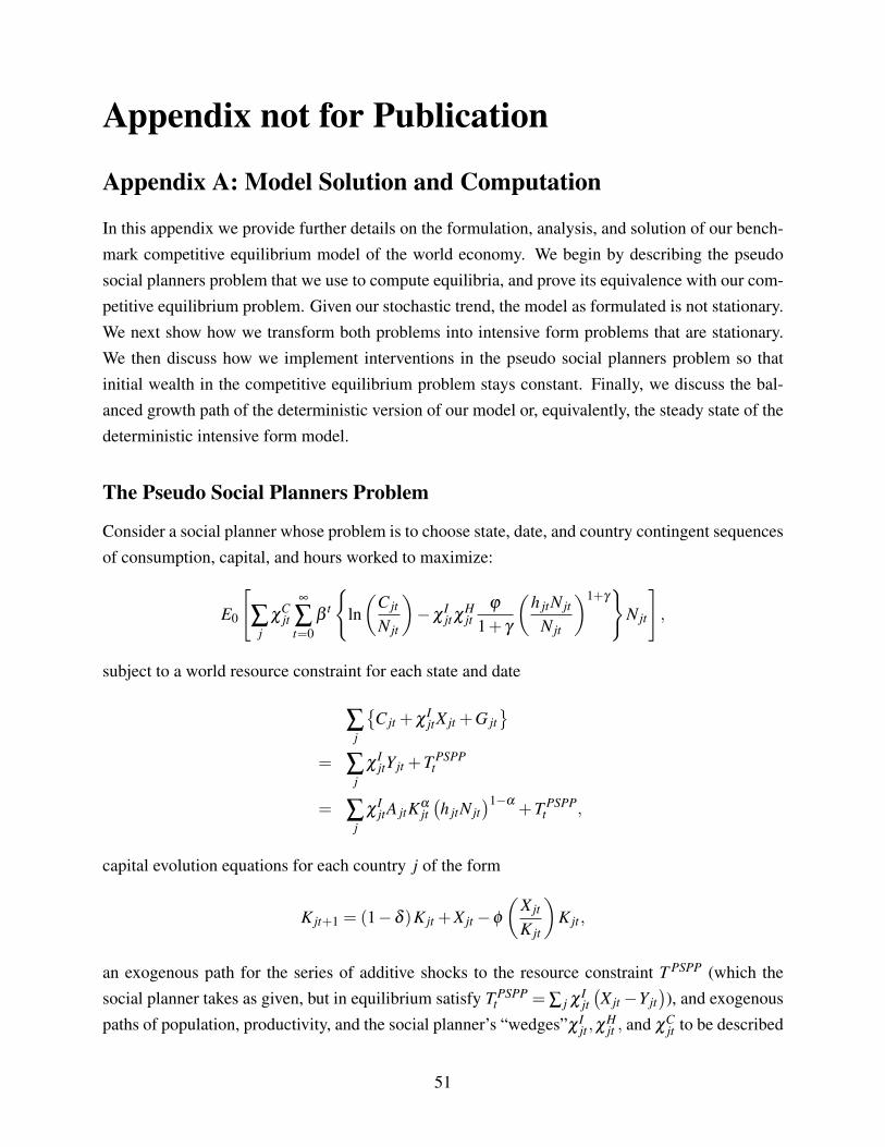
Appendix not for Publication

Appendix A: Model Solution and Computation

In this appendix we provide further details on the formulation, analysis, and solution of our bench-mark competitive equilibrium model of the world economy. We begin by describing the pseudosocial planners problem that we use to compute equilibria, and prove its equivalence with our com-petitive equilibrium problem. Given our stochastic trend, the model as formulated is not stationary.We next show how we transform both problems into intensive form problems that are stationary.We then discuss how we implement interventions in the pseudo social planners problem so thatinitial wealth in the competitive equilibrium problem stays constant. Finally, we discuss the bal-anced growth path of the deterministic version of our model or, equivalently, the steady state of thedeterministic intensive form model.

The Pseudo Social Planners Problem

Consider a social planner whose problem is to choose state, date, and country contingent sequencesof consumption, capital, and hours worked to maximize:

E0

"

Âj

cCjt

•

Ât=0

b t

(ln✓

Cjt

Njt

◆�c I

jt cHjt

j1+ g

✓h jtNjt

Njt

◆1+g)

Njt

#,

subject to a world resource constraint for each state and date

Âj

�Cjt +c I

jtXjt +G jt

= Âj

c IjtYjt +T PSPP

t

= Âj

c IjtA jtKa

jt�h jtNjt

�1�a+T PSPP

t ,

capital evolution equations for each country j of the form

Kjt+1 = (1�d )Kjt +Xjt �f✓

Xjt

Kjt

◆Kjt ,

an exogenous path for the series of additive shocks to the resource constraint T PSPP (which thesocial planner takes as given, but in equilibrium satisfy T PSPP

t = Â j c Ijt�Xjt �Yjt

�), and exogenous

paths of population, productivity, and the social planner’s “wedges”c Ijt ,cH

jt , and cCjt to be described

51

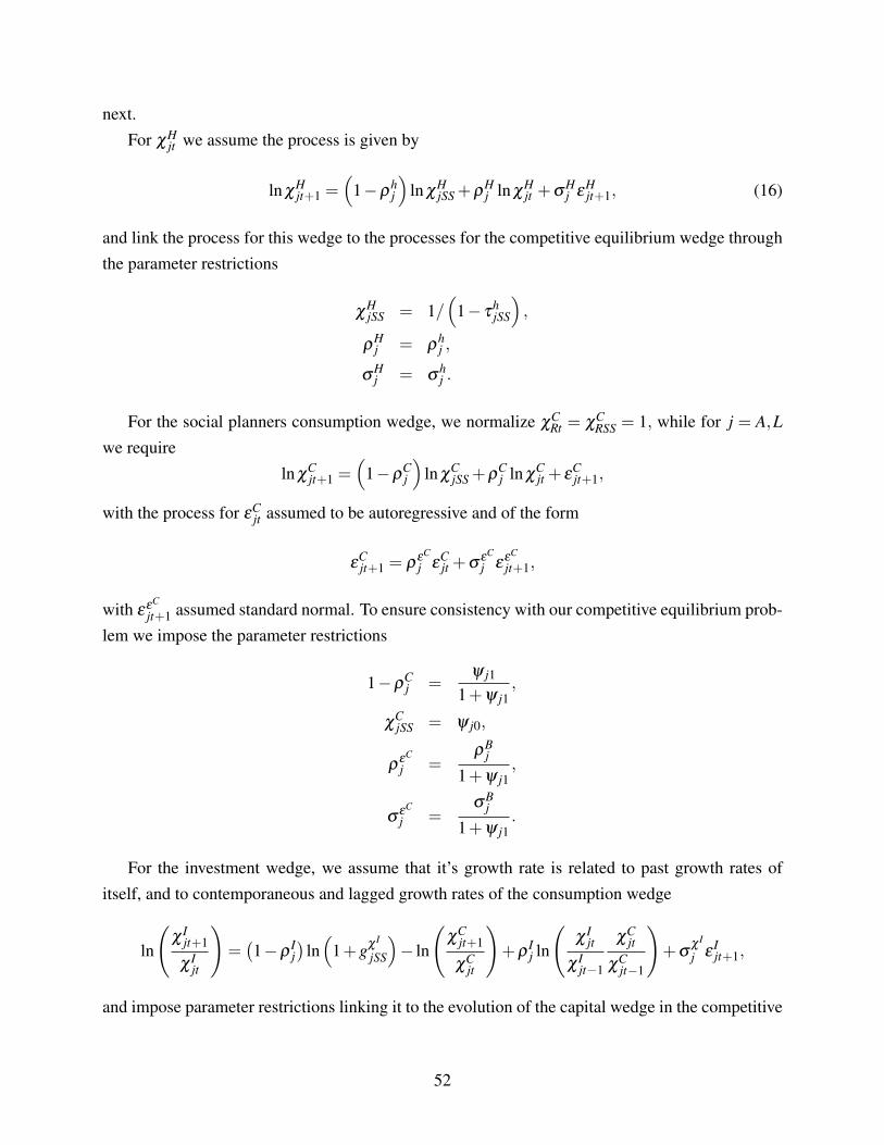
next.For cH

jt we assume the process is given by

ln cHjt+1 =

⇣1�rh

j

⌘ln cH

jSS +rHj ln cH

jt +sHj eH

jt+1, (16)

and link the process for this wedge to the processes for the competitive equilibrium wedge throughthe parameter restrictions

cHjSS = 1/

⇣1� th

jSS

⌘,

rHj = rh

j ,

sHj = sh

j .

For the social planners consumption wedge, we normalize cCRt = cC

RSS = 1, while for j = A,Lwe require

ln cCjt+1 =

⇣1�rC

j

⌘ln cC

jSS +rCj ln cC

jt + eCjt+1,

with the process for eCjt assumed to be autoregressive and of the form

eCjt+1 = reC

j eCjt +seC

j eeC

jt+1,

with eeC

jt+1 assumed standard normal. To ensure consistency with our competitive equilibrium prob-lem we impose the parameter restrictions

1�rCj =

y j1

1+y j1,

cCjSS = y j0,

reC

j =rB

j

1+y j1,

seC

j =sB

j

1+y j1.

For the investment wedge, we assume that it’s growth rate is related to past growth rates ofitself, and to contemporaneous and lagged growth rates of the consumption wedge

ln

c I

jt+1

c Ijt

!=�1�r I

j�

ln⇣

1+gc I

jSS

⌘� ln

cC

jt+1

cCjt

!+r I

j ln

c I

jt

c Ijt�1

cCjt

cCjt�1

!+s c I

j e Ijt+1,

and impose parameter restrictions linking it to the evolution of the capital wedge in the competitive

52

equilibrium problem.

r Ij = rK

j ,

1+gc I

jSS = 1� tKjSS

s c I

j = sKj . (17)

Note that, compared to the competitive equilibrium problem, the formulation of this problem,and the specification of the wedges, is non-standard. As just one example, the investment wedge c I

now appears in the objective function and multiplies both the production function and investmentin the resource constraint. This specification is necessary to recover the competitive equilibrium al-locations. The is quite intuitive: the investment wedge c I must multiply both output and investmentin the resource constraint in order to replicate the capital wedge, which is modeled as a tax on thegross return to capital inclusive of the value of capital, but this causes it to enter the planners opti-mality condition for labor. The addition of the investment wedge as a multiplier on leisure ensuresthat the investment wedge cancels when determining optimal labor supply. As another example,the error term in the social planners consumption wedge is autoregressive. As yet another example,we impose a very precise relationship between the investment wedge and the consumption wedge.As a result of the unusual nature of this formulation, we work with the competitive equilibriumbenchmark in the paper, instead of directly introducing the social planning problem.

Under a restriction on the growth of the world economy (so that the expected summation in theobjective function is finite), this problem is well defined. It is also convex. Hence, the necessaryand sufficient conditions for an optimum include

Cjt : b t cCjt

Njt

Cjt= l PSPP

t , (18)

h jt : b t cCjt cH

jt yhgjt = l PSPP

t (1�a)Yjt

h jtNjt(19)

Kjt+1 : µPSPPjt = E

l PSPP

t+1 c Ijt+1a

Yjt+1

Kjt+1(20)

+µPSPPjt+1

✓1�d �f

✓Xjt+1

Kjt+1

◆+f 0

✓Xjt+1

Kjt+1

◆Xjt+1

Kjt+1

◆�

Xjt : l PSPPt c I

jt = µPSPPjt

✓1�f 0

✓Xjt

Kjt

◆◆(21)

where l PSPPt is the multiplier on the resource constraint at time t and µPSPP

jt the one of the capitalevolution equation in country j at time t.

To establish the legitimacy of using the pseudo social planner to find a solution to the compet-

53

itive equilibrium problem, it is sufficient to show that a solution to these necessary and sufficientconditions is also a solution to the necessary conditions for the competitive equilibrium problem.We do this next.

Equivalence Between the Solution of the Pseudo Social Planner’s Problem andthe Competitive Equilibrium

To establish the legitimacy of using the pseudo social planner’s problem (PSPP) to find a solutionto the competitive equilibrium problem (CEP), we need to show that the solution to the necessaryand sufficient conditions for an optimum of the PSPP is also a solution to the necessary conditionsfor the competitive equilibrium problem. For this, it is sufficient to exhibit both the prices and theLagrange multipliers that ensure that the optimality conditions from the CEP are satisfied.

Consider the first order condition (FOC) of the PSPP with respect to consumption (18). Thecorresponding FOC of the households problem from the CEP is

b t Njt

Cjt= l HH

jt ,

and so the two conditions are equivalent iff

l HHjt =

l PSPPt

cCjt

. (22)

Likewise, the FOC of the PSPP with respect to hours (19) can be compared with the correspondingFOC of the households problem from the CEP

b tyhgjt = l HH

jt

⇣1� th

jt

⌘Wjt .

Hence, the two conditions are equivalent iff

l HHjt

⇣1� th

jt

⌘Wjt =

l PSPPt

cCjt

1cH

jt(1�a)

Yjt

h jtNjt.

But imposing (22), we can see that the conditions will be equivalent if

Wjt = (1�a)Yjt

h jtNjt, (23)

1� thjt =

1cH

jt. (24)

54

Note that (23) implies that the FOC in hours for the firm producing the consumption good inthe CEP is now satisfied. Moreover, given assumption (16), the derived process for 1�th

jt satisfiedthe law of motion (8) from the CEP because

ln cHjt+1 =

⇣1�rh

j

⌘ln cH

jSS +rHj ln cH

jt +sHj eH

jt+1,

becomesln⇣

1� thjt+1

⌘=⇣

1�rhj

⌘ln⇣

1� thjSS

⌘+rh

j ln⇣

1� thjt

⌘+sh

j ehjt+1,

under our assumptions on parameters above with eHjt+1 =�eh

jt+1.

The FOCs of the PSPP in consumption for country j and the rest of the world can be combinedto yield

Cjt/Njt

CRt/NRt=

cCjt

cCRt.

Under our normalization and parameter restrictions, this implies

lnCjt+1/Njt+1

CRt+1/NRt+1=

y j1

1+y j1lny j0 +

11+y j1

lnCjt/Njt

CRt/NRt+ eC

jt+1,

which is precisely equation (12) from the CEP problem with eCjt+1 = ln

⇣1� t⇤B

jt+1

⌘.

The FOC with respect to capital from the PSPP (20) combined with the FOC with respect toinvestment (21) can be rearranged to yield

l PSPPt c I

jt

1�f 0⇣

XjtKjt

⌘ = Et

2

4l PSPPt+1 c I

jt+1

0

@aYjt+1

Kjt+1+

1�d �f⇣

Xjt+1Kjt+1

⌘+f 0

⇣Xjt+1Kjt+1

⌘Xjt+1Kjt+1

1�f 0⇣

Xjt+1Kjt+1

⌘

1

A

3

5 .

Comparing this with the FOC in capital from the households problem

l HHjt PK

jt = Et⇥l HH

jt+1�1� tK

jt+1��

rKjt+1 +P⇤K

jt+1�⇤,

we can see that the two will be equivalent if

rKjt+1 = a

Yjt+1

Kjt+1,

PKjt =

1

1�f 0⇣

XjtKjt

⌘ ,

P⇤Kjt+1 =

1�d �f⇣

Xjt+1Kjt+1

⌘+f 0

⇣Xjt+1Kjt+1

⌘Xjt+1Kjt+1

1�f 0⇣

Xjt+1Kjt+1

⌘ ,

55

1� tKjt+1 =

cCjt+1

cCjt

c Ijt+1

c Ijt

, (25)

where in the last line we substituted from (22). The first of these conditions is simply the FOC incapital for the firm producing the consumption good in the CEP, while the second and third are theoptimality conditions for the firm producing the capital good.

The fourth line gives us the relationship between the consumption and investment wedges inthe PSPP and the capital wedge from the CEP. This is straightforward to impose in our analysis;for any process for the growth of the PSPP consumption wedge, we simply implicitly assumewhatever process for the growth of the PSPP investment wedge necessary to generate a first orderautoregressive process for the product of its growth rate with that of the consumption wedge. Tosee that the conditions presented above are sufficient to ensure that this is true, note that under thisrestriction we have

ln�1� tK

jt+1�= ln

�c I

jt+1/c Ijt�+ ln

⇣cC

jt+1/cCjt

⌘,

so that after substituting for (25) and imposing the restrictions in (17) we obtain the evolutionequation for the capital wedge in the CEP

ln�1� tK

jt+1�=�1�rK

j�

ln�1� tK

jSS�+rK

j ln�1� tK

jt�+sK

j eKjt+1.

Lastly, note that the resource constraint of the PSPP is equal to the sum of the budget constraintsof the CE problem after imposing market clearing in bonds. Or, conversely, substituting for theallocations, prices and transfers in the CEP budget constraints from the PSPP problem, we candeduce the implied sequences of foreign bond holdings.

The Intensive Form Problem

Recall that, as discussed in Section 2.3 of the text, the world economy is assumed to follow astochastic trend identified with the rest of the world’s level of effective labor Zt = A1/(1�a)

Rt NRt . Asthe trend possesses a unit root, to make the model stationary we will work with first differences ofthis trend zt+1 = Zt+1/Zt and scale all variables by the level of effective labor in the previous periodZt�1. We also define

pt+1 =ARt+1

ARt,

ht+1 =NRt+1

NRt,

56

so that

zt+1 =Zt+1

Zt=

A1/(1�a)Rt+1 NRt+1

A1/(1�a)Rt NRt

= p1/(1�a)t+1 ht+1.

For notational simplicity it also helps to define aRt = nRt = 1 for all t in all states.This section outlines this process and derives the resulting intensive form competitive equilib-

rium. We also derive the intensive form social planning problem that is the basis for our numericalalgorithm and estimation. In the next section, we use the intensive form versions of both problemsto establish that solutions to the pseudo social planner’s problem are also competitive equilibria.

Competitive Equilibrium Problem

Recall that the problem of country j is to maximize

E0

"•

Ât=0

b t⇢

ln✓

Cjt

Njt

◆� y

1+ gh1+g

jt

�Njt

#,

subject to a flow budget constraint for each state and date

Cjt +PKjt Kjt+1 +Et

⇥qt+1B jt+1

⇤

⇣1� th

jt

⌘Wjth jtNjt +

�1� tB

jt +Y jt�

B jt +Tjt

+�1� tK

jt��

rKjt +P⇤K

jt�

Kjt ,

where, from the perspective of the country, Y jt is a fixed sequence of interest penalties (analogousto a debt elastic interest rate that is not internalized) and where PK

jt is the price of new capital goods,and P⇤K

jt is the price of old capital goods.Substituting for the evolution of the exogenous states and scaling by Zt�1, and denoting all

scaled variables by lower case, yields for the household’s objective function

E0

"•

Ât=0

b t

t

’s=0

hs

!⇢ln✓

Cjt

Njt

◆� y

1+ gh1+g

jt

�n jtNR0

#,

which is an affine transformation of

E0

"•

Ât=0

b t

t

’s=0

hs

!⇢ln�c jt�� y

1+ gh1+g

jt

�n jt

#.

For the household budget constraint we get

c jt +PKjt ztk jt+1 + ztEt

⇥qt+1b jt+1

⇤

⇣1� th

jt

⌘ Wjth jtNjt

A1/(1�a)Rt�1 NRt�1

+�1� tB

jt +Y jt�

b jt + t jt

57

+�1� tK

jt��

rKjt +P⇤K

jt�

k jt .

Recall that there are two types of firm in this economy. The first produces the final consumptiongood. Optimization for these firms implies that

Wjt = (1�a)A jt

✓Kjt

h jtNjt

◆a,

rKjt = aA jt

✓Kjt

h jtNjt

◆�(1�a)

.

Noting that

Wjt = (1�a)A jt

✓Kjt

h jtNjt

◆a

= (1�a)a jtARt

✓Kjt

ht jn jtNRt

◆a,

we let

w jt =Wjt

A1/(1�a)Rt�1

= (1�a)a jt

Kjt

ht jn jtA1/(1�a)Rt�1 NRt

!a

= (1�a)a jtpt

✓k jt

h jtn jtht

◆a.

But note that for the return to capital

rKjt = aA jt

✓Kjt

h jtNjt

◆�(1�a)

= aa jtARt

✓Kjt

h jtn jtNRt

◆�(1�a)

= aa jtARt

Kjt

h jtn jtA1/(1�a)Rt�1 NRt�1

A1/(1�a)Rt�1 NRt�1

NRt

!�(1�a)

= aa jtpt

✓k jt

h jtn jtht

◆�(1�a)

,

so that no scaling of capital returns is required.The second type of firm produces new capital goods ztk jt+1 using x jt units of deferred con-

58

sumption and k jt units of the old capital good. Their objective function is

PKjt ztk jt+1 � x jt �P⇤K

jt k jt .

Assuming a capital accumulation equation with adjustment costs of the form

ztk jt+1 = (1�d )k jt + x jt �f✓

x jt

k jt

◆k jt ,

we get that the firms problem is to choose x jt and k jt to maximize

PKjt

(1�d )k jt + x jt �f

✓x jt

k jt

◆k jt

�� x jt �P⇤K

jt k jt .

The FOC in x implies

PKjt =

1

1�f 0⇣

x jtk jt

⌘ ,

while the one in k yields

P⇤Kjt = PK

jt

✓1�d �f

✓x jt

k jt

◆+f 0

✓x jt

k jt

◆x jt

k jt

◆.

The first order conditions of the household’s intensive form problem are

c jt : b t

t

’s=0

hs

!n jt

1c jt

= lCEjt ,

h jt : b t

t

’s=0

hs

!n jtyhg

jt = lCEjt

⇣1� th

jt

⌘w jtn jtht ,

k jt+1 : 1 = E

"lCE

jt+1

lCEjt

�1� tK

jt+1� rK

jt+1 +P⇤Kjt+1

PKjt zt

#,

b jt+1 : ztqt+1lCEjt = lCE

jt+1⇥�

1� tBjt+1 +Y jt+1

�⇤,

where lCEjt is the multiplier on the budget constraint.

If transfers rebate all “tax revenues” beyond that required to finance government expenditure,then in equilibrium we have

c jt + ztk jt+1 + ztEt⇥qt+1b jt+1

⇤+g jt = w jth jtn jtht +

�rK

jt +1�d�

k jt �f✓

x jt

k jt

◆k jt +b jt .

59

From the labor-leisure condition we get

yhgjt =

1c jt

⇣1� th

jt

⌘w jtn jtht .

From the Euler equation in physical capital we get

1 = E

2

64lCE

jt+1

lCEjt

�1� tK

jt+1� rK

jt+1 +⇣

1�d �f⇣

x jt+1k jt+1

⌘+f 0

⇣x jt+1k jt+1

⌘x jt+1k jt+1

⌘/⇣

1�f 0⇣

x jt+1k jt+1

⌘⌘

zt

⇣1�f 0

⇣x jtk jt

⌘⌘�1

3

75 .

After substituting for lCE we obtain

1=E

2

64bht+1c jt

c jt+1

n jt+1

n jt

�1� tK

jt+1� rK

jt+1 +⇣

1�d �f⇣

x jt+1k jt+1

⌘+f 0

⇣x jt+1k jt+1

⌘x jt+1k jt+1

⌘/⇣

1�f 0⇣

x jt+1k jt+1

⌘⌘

zt

⇣1�f 0

⇣x jtk jt

⌘⌘�1

3

75 .

Lastly, from the Euler equation in foreign assets, we obtain

ztqt+1n jt

c jt= bht

n jt+1

c jt+1

�1� tB

jt ++Y jt�.

Pseudo Social Planners Problem

Following an analogous process for the pseudo social planner’s problem introduced above, theintensive form pseudo social planners objective function becomes

E0

"

Âj

cCjt

•

Ât=0

b t⇢

ln✓

Cjt

Njt

◆�c I

jt cHjt

y1+ g

h1+gjt

�n jtNRt

#

= E0

"

Âj

cCjt

•

Ât=0

b t

t

’s=0

hs

!⇢ln✓

Cjt

Njt

◆�c I

jt cHjt

y1+ g

h1+gjt

�n jtNR0

#,

which is equivalent to maximizing

E0

"•

Ât=0

b t

t

’s=0

hs

!

Âj

cCjt

⇢ln�c jt��c I

jt cHjt

y1+ g

h1+gjt

�n jt

#.

The resource constraint becomes

Âj

�c jt +c I

jtx jt +g jt

60

= Âj

c Ijty jt + tSP

t

= Âj

c Ijta jtptka

jt�h jtn jtht

�1�a+ tSP

t ,

while the capital evolution equation is

ztk jt+1 = (1�d )k jt + x jt �f✓

x jt

k jt

◆k jt .

The first order conditions of this problem are

c jt : b t

t

’s=0

hs

!cC

jt1

c jtn jt = l SP

t ,

h jt : b t

t

’s=0

hs

!cC

jt c Ijt cH

jt yhgjtn jt = l SP

t (1�a)c Ijta jtptn jthtka

jt�h jtn jtht

��a

k jt+1 : µSPjt zt = E

hl SP

t+1c Ijt+1aa jt+1pt+1ka�1

jt+1�h jt+1n jt+1ht+1

�1�a+

µSPjt+1

✓1�d �f

✓x jt+1

k jt+1

◆+f 0

✓x jt+1

k jt+1

◆x jt+1

k jt+1

◆�,

x jt : l SPt c I

jt = µSPjt

✓1�f 0

✓x jt

k jt

◆◆,

where l SPt is the multiplier on the resource constraint at time t and µSP

jt the one of the capitalevolution equation in country j at time t. We can rearrange these, after substituting for l SP

t , to get

1 = E

"bht+1

c jt

c jt+1

n jt

n jt+1

cCt+1

cCt

c Ijt+1

c Ijt

⇥

aa jt+1pt+1ka�1jt+1�h jt+1n jt+1ht+1

�1�a+⇣

1�d �f⇣

x jt+1k jt+1

⌘+f 0

⇣x jt+1k jt+1

⌘x jt+1k jt+1

⌘/⇣

1�f 0⇣

x jt+1k jt+1

⌘⌘

zt

⇣1�f 0

⇣x jtk jt

⌘⌘

3

5 .

Imposing the “equilibrium” restriction on the wedges and additive shock yields

Âj

⇢c jt + ztk jt+1 � (1�d )kt �f

✓x jt

k jt

◆k jt +g jt

�= Â

ja jtptka

jt�h jtn jtht

�1�a.

61

The Equivalence of Interventions in the Competitive Equilibrium and PseudoSocial Planner’s Problems

In the paper, we aim to quantify the contributions of the different wedges to capital flows by con-ducting a particular set of interventions. Specifically, we set the wedge in question equal to itsaverage level, and then track how capital flows evolve under this intervention. In the competitiveequilibrium problem, this change would occur for a given level of initial wealth or net foreign as-sets. However, as we use a pseudo social planners problem to solve and estimate the equilibrium,and simulate the effect of an intervention, we need to change the level of the Pareto weight (the so-cial planning analog of initial wealth) or, equivalently, the initial level of the pseudo social planner’sinternational wedge, so as to keep wealth in the competitive equilibrium problem constant. This isdone by allowing the initial values of the pseudo social planner’s international wedge (equivalently,the planner’s Pareto weight) to jump to the level required to keep net foreign assets constant.

To see how we do this, note that in the competitive equilibrium problem at the beginning ofperiod t after the resolution of uncertainty, the j0th country’s net foreign asset position is given bythe number B jt . From the resource constraint we know that

B jt =�NXjt +Et⇥qt,t+1B jt+1

⇤.

We also know, from the Euler equation in bonds, that for j = ROW (with no taxes)

1Cjt

Njtqt,t+1 = b 1Cjt+1

Njt+1.

Substituting gives

B jt = �NXjt +Et

b CRt

CRt+1

NRt+1

NRtB jt+1

�

= �NXjt +Et

b CRt

CRt+1ht+1B jt+1

�.

The intensive form analog is then

B jt

Zt�1=�

NXjt

Zt�1+Et

b CRt/Zt�1

CRt+1/Zt

Zt�1

Ztht+1

B jt+1

Zt

Zt

Zt�1

�,

so thatb jt =�nx jt +Et

b cRt

cRt+1ht+1b jt+1

�,

62

which after recursively substituting becomes

b jt = �Et

⇢nx jt +bht+1

cRt

cRt+1nx jt+1 +b 2ht+1ht+2

cRt

cRt+2nx jt+2 + ...

�

= �Et

(•

Âs=0

b s

s

’r=1

ht+r

!nx jt+s

), (26)

where1

’s=0

ht+r = 1.

In solving the pseudo social planners problem, we compute the solution for net foreign assetsas a function of the state (which includes the pseudo social planner’s international wedge) usingequation (26), which allows us to numerically vary the level of the social planner’s internationalwedge in order to keep net foreign assets constant.

The Balanced Growth Path of the Deterministic Model

In this section we derive the balanced growth path of our model or, equivalently, the steady stateof the intensive form version of our model. We then use this derivation to go into further detailabout why we needed to add the portfolio adjustment costs in order to establish the existence of anon-degenerate balanced growth path for our model. Lastly, we use the derivation to show why thelabor wedge has little role on the balanced growth path of the model, even though it matters a greatdeal along the transition to this balanced growth path, and hence why analyses based on steady staterelations will tend to understate the importance of the labor wedge in determining capital flows.

As noted in the text, which can be easily verified from the resource constraint of the econ-omy, along the balanced growth path the growth rates of consumption, investment, capital, output,government spending and net exports for all countries are all equal to the long run growth rate ofeffective labor, or

zss = hssp1

1�ass .

From the household’s optimality condition in the accumulation of international assets, we can seethat on the balanced growth path the price of these assets satisfies

11+ rW

ss⌘ qss = b hss

zss= bp

�11�ass ,

where we have defined rWss to be the steady state world interest rate. That is, as usual, the world

interest rate increases in the discount rate (decreases in the discount factor) and increases in the rateof growth of productivity.

63

As far as country specific levels of variables, the steady state level of government spendingrelative to output is given by assumption as g jss. Steady state investment relative to capital is deter-mined from the capital accumulation equation to be

✓Xj

Kj

◆

ss= d + zss �1,

where we have imposed the fact that adjustment costs are zero on the balanced growth path (orsteady state), and where we have written the subscript “ss” outside of the parentheses to denote thefact that the ratio of investment to capital is constant on the balanced growth path, but the levels ofinvestment and capital themselves are not. Hence, investment relative to output is given by

✓Xj

Yj

◆

ss= (d + zss �1)

✓Kj

Yj

◆

ss,

and so will be pinned down once we know the steady state output to capital ratio.From the Euler equation in capital, imposing steady state, we have

1+ rWss =

�1� tK

jss�✓

a✓

Yj

Kj

◆

ss+1�d

◆

which pins down the capital to output ratio as

Kjss

Yjss= a 1

1+rWss

1�tKjss� (1�d )

.

All that remains is to pin down is consumption, hours, net exports and net foreign assets on thebalanced growth path. It turns out that all of this can be done once we have the level of net foreignassets relative to output. Given

�B j/Yj

�ss we have that

✓B j

Yj

◆

ss(1�qzss) =�

✓NXj

Yj

◆

ss.

This simply states that the level of net exports in steady state is equal to the growth adjusted worldinterest rate on net foreign assets.

As an aside, it is worthwhile to note that, since net foreign assets are growing on the balancedgrowth path, the current account—in a deterministic model, this is equal to the change in the levelof net foreign assets—is not zero on the balanced growth path. Given our timing convention, the

64

ratio of the current account CA to output is given by

✓CA j

Yj

◆

ss=

B0

j �B j

Yj

!

ss

= (zss �1)✓

B j

Yj

◆

ss=

1� zss

1�qzss

✓NXj

Yj

◆

ss.

Given the ratio of net exports to output, we can back out the ratio of consumption to outputfrom the resource constraint of a country

✓Cj

Yj

◆

ss= 1�

✓Xj

Yj

◆

ss�g jss �

✓NXj

Yj

◆

ss.

The level of hours per person (which is constant on the balanced growth path) is then pinned downby the first order condition in hours

h jss =

1� th

jss

y

✓Yj

Cj

◆

ss

!1/(1+g)

.

What determines the level of net foreign assets relative to output on the balanced growth path?In a complete markets model without wedges, this would be pinned down by initial conditions. Inan incomplete markets model, in general, this level would not be pinned down at all, but wouldinstead vary forever with the sequence of shocks that hit the economy. This is why the modeldoes not possess a unique steady state: if the shocks are all set to zero after some date T, and theeconomy jumped immediately to the balance growth path, the level of net foreign assets that hadbeen accumulated up until that time period, scaled by output, would persist forever after. This iswhy we, and all of the literature up until this point, has adopted some mechanism for pinning downthe long run level of net foreign assets relative to output. Our specification of a tax on deviations ofnet foreign assets from a benchmark allows us to estimate the balanced growth path of assets fromthe data.

It is also worth pointing out that, as constructed above, the labor wedge had no impact on thebalanced growth path except for determining the level of hours worked relative to consumption.This is a little misleading; in general, realizations of the labor wedge will affect the economy onthe transition to steady state and hence will affect the accumulation of net foreign assets. However,analysis of capital flows from the balanced growth perspective, that ignores the transition path, willfind no role for the labor wedge to impact long run capital flows.

65

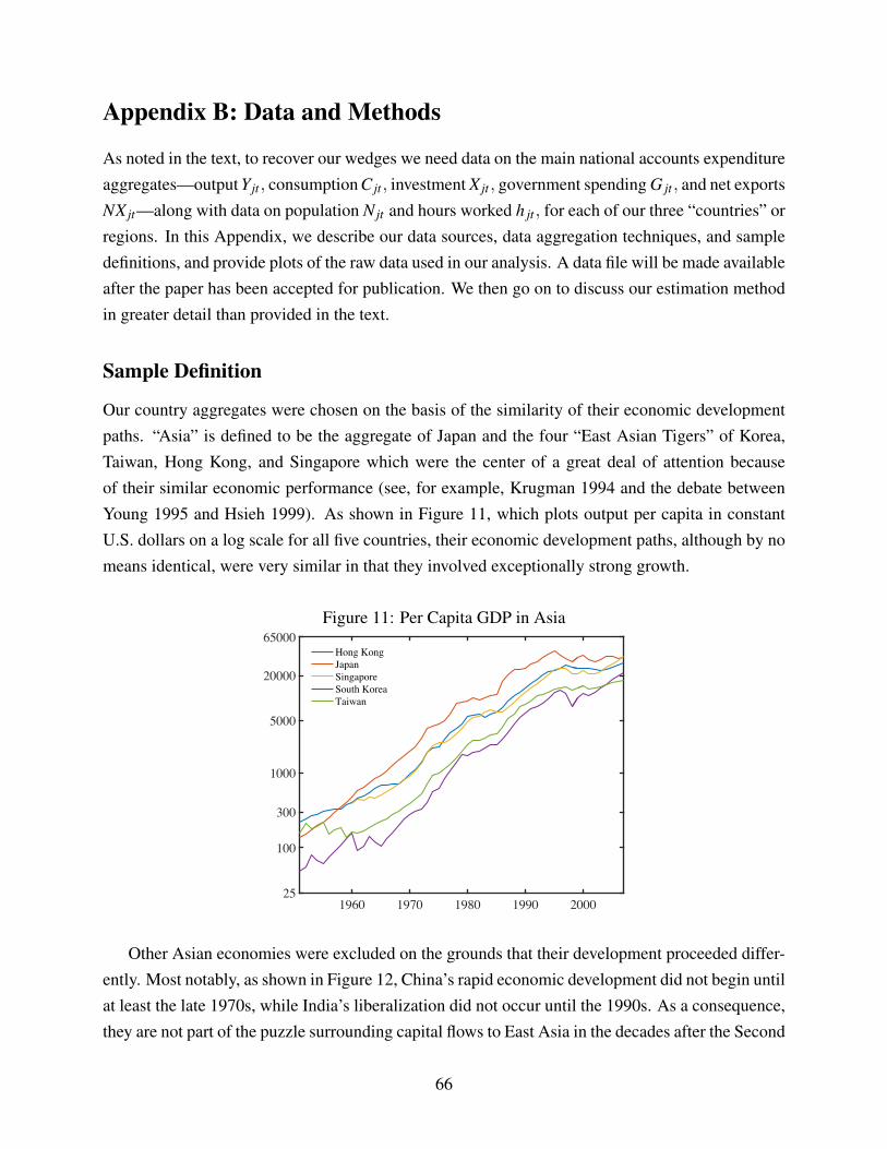
Appendix B: Data and Methods

As noted in the text, to recover our wedges we need data on the main national accounts expenditureaggregates—output Yjt , consumption Cjt , investment Xjt , government spending G jt , and net exportsNXjt—along with data on population Njt and hours worked h jt , for each of our three “countries” orregions. In this Appendix, we describe our data sources, data aggregation techniques, and sampledefinitions, and provide plots of the raw data used in our analysis. A data file will be made availableafter the paper has been accepted for publication. We then go on to discuss our estimation methodin greater detail than provided in the text.

Sample Definition

Our country aggregates were chosen on the basis of the similarity of their economic developmentpaths. “Asia” is defined to be the aggregate of Japan and the four “East Asian Tigers” of Korea,Taiwan, Hong Kong, and Singapore which were the center of a great deal of attention becauseof their similar economic performance (see, for example, Krugman 1994 and the debate betweenYoung 1995 and Hsieh 1999). As shown in Figure 11, which plots output per capita in constantU.S. dollars on a log scale for all five countries, their economic development paths, although by nomeans identical, were very similar in that they involved exceptionally strong growth.

Figure 11: Per Capita GDP in Asia

1960 1970 1980 1990 200025

100

300

1000

5000

20000

65000Hong KongJapanSingaporeSouth KoreaTaiwan

Other Asian economies were excluded on the grounds that their development proceeded differ-ently. Most notably, as shown in Figure 12, China’s rapid economic development did not begin untilat least the late 1970s, while India’s liberalization did not occur until the 1990s. As a consequence,they are not part of the puzzle surrounding capital flows to East Asia in the decades after the Second

66

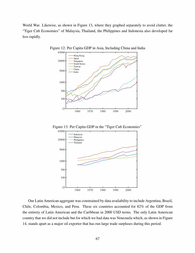
World War. Likewise, as shown in Figure 13, where they graphed separately to avoid clutter, the“Tiger Cub Economies” of Malaysia, Thailand, the Philippines and Indonesia also developed farless rapidly.

Figure 12: Per Capita GDP in Asia, Including China and India

1960 1970 1980 1990 200025

100

300

1000

5000

20000

65000Hong KongJapanSingaporeSouth KoreaTaiwanChinaIndia

Figure 13: Per Capita GDP in the “Tiger Cub Economies”

1960 1970 1980 1990 200025

100

300

1000

5000

20000

65000IndonesiaMalaysiaPhilippinesThailand

Our Latin American aggregate was constrained by data availability to include Argentina, Brazil,Chile, Colombia, Mexico, and Peru. These six countries accounted for 82% of the GDP fromthe entirety of Latin American and the Caribbean in 2000 USD terms. The only Latin Americancountry that we did not include but for which we had data was Venezuela which, as shown in Figure14, stands apart as a major oil exporter that has run large trade surpluses during this period.

67

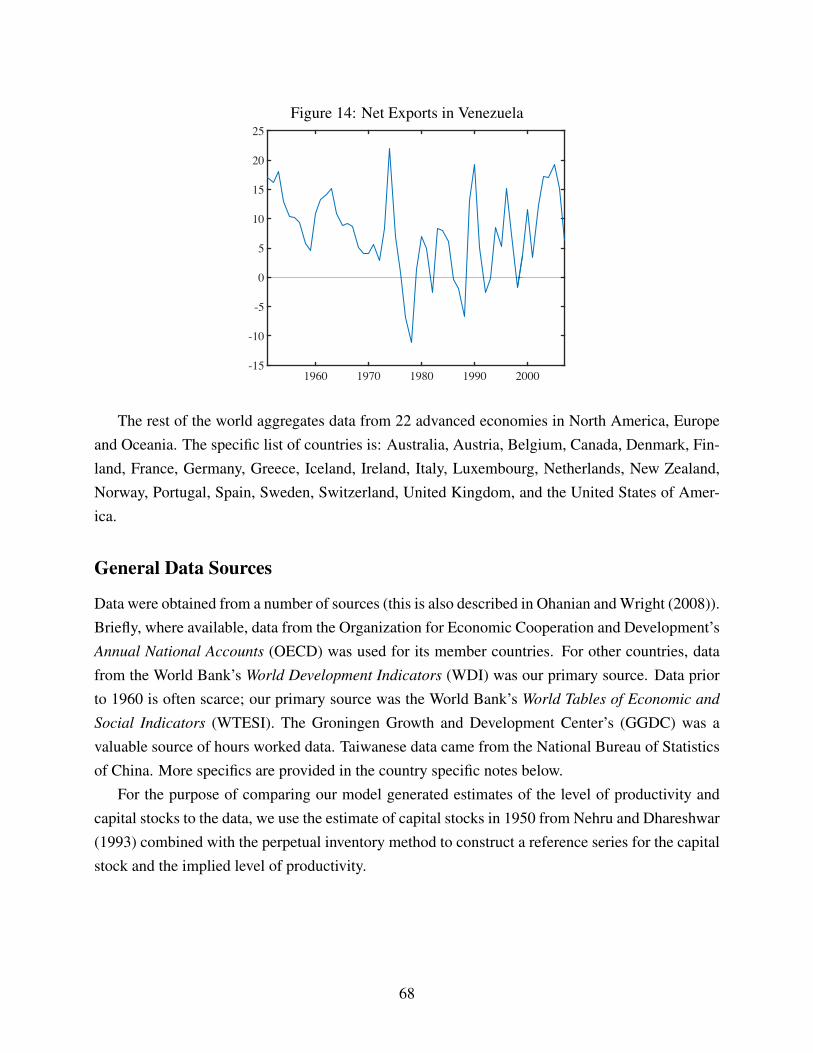
Figure 14: Net Exports in Venezuela

1960 1970 1980 1990 2000-15

-10

-5

0

5

10

15

20

25

The rest of the world aggregates data from 22 advanced economies in North America, Europeand Oceania. The specific list of countries is: Australia, Austria, Belgium, Canada, Denmark, Fin-land, France, Germany, Greece, Iceland, Ireland, Italy, Luxembourg, Netherlands, New Zealand,Norway, Portugal, Spain, Sweden, Switzerland, United Kingdom, and the United States of Amer-ica.

General Data Sources

Data were obtained from a number of sources (this is also described in Ohanian and Wright (2008)).Briefly, where available, data from the Organization for Economic Cooperation and Development’sAnnual National Accounts (OECD) was used for its member countries. For other countries, datafrom the World Bank’s World Development Indicators (WDI) was our primary source. Data priorto 1960 is often scarce; our primary source was the World Bank’s World Tables of Economic andSocial Indicators (WTESI). The Groningen Growth and Development Center’s (GGDC) was avaluable source of hours worked data. Taiwanese data came from the National Bureau of Statisticsof China. More specifics are provided in the country specific notes below.

For the purpose of comparing our model generated estimates of the level of productivity andcapital stocks to the data, we use the estimate of capital stocks in 1950 from Nehru and Dhareshwar(1993) combined with the perpetual inventory method to construct a reference series for the capitalstock and the implied level of productivity.

68

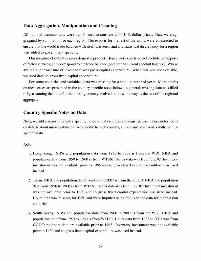
Data Aggregation, Manipulation and Cleaning

All national accounts data were transformed to constant 2000 U.S. dollar prices. Data were ag-gregated by summation for each region. Net exports for the rest of the world were constructed toensure that the world trade balance with itself was zero, and any statistical discrepancy for a regionwas added to government spending.

Our measure of output is gross domestic product. Hence, net exports do not include net exportsof factor services, and correspond to the trade balance (and not the current account balance). Whereavailable, our measure of investment was gross capital expenditure. When this was not available,we used data on gross fixed capital expenditure.

For some countries and variables, data was missing for a small number of years. More detailson these cases are presented in the country specific notes below; in general, missing data was filledin by assuming that data for the missing country evolved in the same way as the rest of the regionalaggregate.

Country Specific Notes on Data

Next, we add a series of country specific notes on data sources and construction. These notes focuson details about missing data that are specific to each country, and on any other issues with countryspecific data.

Asia

1. Hong Kong. NIPA and population data from 1960 to 2007 is from the WDI. NIPA andpopulation data from 1950 to 1960 is from WTESI. Hours data was from GGDC. Inventoryinvestment was not available prior to 1965 and so gross fixed capital expenditure was usedinstead.

2. Japan. NIPA and population data from 1960 to 2007 is from the OECD. NIPA and populationdata from 1950 to 1960 is from WTESI. Hours data was from GGDC. Inventory investmentwas not available prior to 1960 and so gross fixed capital expenditure was used instead.Hours data was missing for 1950 and were imputed using trends in the data for other Asiancountries.

3. South Korea. NIPA and population data from 1960 to 2007 is from the WDI. NIPA andpopulation data from 1950 to 1960 is from WTESI. Hours data from 1963 to 2007 was fromGGDC; no hours data are available prior to 1963. Inventory investment was not availableprior to 1960 and so gross fixed capital expenditure was used instead.

69

4. Singapore. Official NIPA data for Singapore first becomes available in 1960 and was takenfrom the WDI. Prior to 1960, NIPA estimates derived from colonial data were obtained fromSugimoto (2011). Hours worked data were taken from GGDC from 1960. Prior to 1960, wecomputed total hours worked from data on the employment and hours worked of laborers,shop assistants, shop clerks and industrial clerks in both public and private sector estab-lishments as tabulated in the Annual Report of the Labour Department for the Colony ofSingapore (1950-1956) and State of Singapore (1957-1960).

5. Taiwan. NIPA data for Taiwan begins in 1951 and comes from the National Bureau of Statis-tics of China. Hours worked data comes from GGDC starting in 1960. Population, and hoursworked data prior to 1960, come from the Penn World Tables v.9.0.

Latin America

1. Argentina. NIPA and population data from 1960 to 2007 is from the WDI. NIPA and pop-ulation data from 1950 to 1960 is from WTESI. Hours data was from GGDC. Inventoryinvestment was not available prior to 1960, and for some years after 1979, and so gross fixedcapital expenditure was used instead.

2. Brazil. NIPA and population data from 1960 to 2007 is from the WDI. NIPA and populationdata from 1950 to 1960 is from WTESI. Hours data was from GGDC. Inventory investmentwas not available prior to 1960 and so gross fixed capital expenditure was used instead.

3. Chile. NIPA and population data from 1960 to 2007 is from the WDI. NIPA and populationdata from 1950 to 1960 is from WTESI. Hours data was from GGDC.

4. Colombia. NIPA and population data from 1960 to 2007 is from the WDI. NIPA and pop-ulation data from 1950 to 1960 is from WTESI. Hours data was from GGDC. Inventoryinvestment was not available prior to 1960 and so gross fixed capital expenditure was usedinstead.

5. Mexico. NIPA and population data from 1960 to 2007 is from the WDI. NIPA and populationdata from 1950 to 1960 is from WTESI. Hours data was from GGDC. Inventory investmentwas not available prior to 1960 and so gross fixed capital expenditure was used instead.

6. Peru. NIPA and population data from 1960 to 2007 is from the WDI. NIPA and populationdata from 1950 to 1960 is from WTESI. Hours data was from GGDC. Inventory investmentwas not available prior to 1960 and so gross fixed capital expenditure was used instead.

70

Rest of the World

We end up with an aggregate of 22 advanced economies from North America, Europe and Aus-tralasia. The specific list of countries is: Australia, Austria, Belgium, Canada, Denmark, Finland,France, Germany, Greece, Iceland, Ireland, Italy, Luxembourg, Netherlands, New Zealand, Nor-way, Portugal, Spain, Sweden, Switzerland, United Kingdom, and the United States of America.

1. Australia. NIPA and population data are from the OECD. Hours worked were taken fromGGDC back until 1953, and extended back to 1950 using the series in Butlin (1977).

2. Austria. NIPA and population data are from the OECD. Hours worked were taken fromGGDC.

3. Belgium. NIPA and population data are from the OECD. Hours worked were taken fromGGDC.

4. Canada. NIPA and population data are from the OECD. Hours worked were taken fromGGDC.

5. Denmark. NIPA and population data are from the OECD. Hours worked were taken fromGGDC.

6. Finland. NIPA and population data are from the OECD. Hours worked were taken fromGGDC.

7. France. NIPA and population data are from the OECD. Hours worked were taken fromGGDC.

8. Germany. NIPA and population data are from the OECD. Hours worked were taken fromGGDC.

9. Greece. NIPA and population data are from the OECD. Hours worked were taken fromGGDC.

10. Iceland. NIPA and population data are from the OECD. Hours worked were taken fromGGDC.

11. Ireland. NIPA and population data are from the OECD. Hours worked were taken fromGGDC.

12. Italy. NIPA and population data are from the OECD. Hours worked were taken from GGDC.

71

13. Luxembourg. NIPA and population data are from the OECD. Hours worked were taken fromGGDC back until 1958.

14. Netherlands. NIPA and population data are from the OECD. Hours worked were taken fromGGDC.

15. New Zealand. NIPA and population data are from the OECD. Hours worked were taken fromGGDC.

16. Norway. NIPA and population data are from the OECD. Hours worked were taken fromGGDC.

17. Portugal. NIPA and population data are from the OECD. Hours worked were taken fromGGDC back until 1956.

18. Spain. NIPA and population data are from the OECD. Hours worked were taken from GGDCback until 1954.

19. Sweden. NIPA and population data are from the OECD. Hours worked were taken fromGGDC back until 1959.

20. Switzerland. NIPA and population data are from the OECD. Hours worked were taken fromGGDC.

21. United Kingdom. NIPA and population data are from the OECD. Hours worked were takenfrom GGDC.

22. The United States of America. NIPA and population data are from the OECD. Hours workedwere taken from GGDC.

Resulting Aggregate Data for the Three Regions

Figures 15 to 18 show plots of the data used in the estimation in natural logs for the first 3 figures(in billions of year 2000 USD) and in millions of people for population. Recall that data on theratio of net exports to income is plotted in Figure 1 in the text, hours worked per capita are plottedin Figure 4, and that government spending was computed as a residual including any statisticaldiscrepancy.

72

Figure 15: Gross Domestic Product

1960 1970 1980 1990 2000100

1000

10000

30000

Rest of the WorldLatin AmericaAsia

Figure 16: Consumption

1960 1970 1980 1990 2000100

250

500

1000

5000

20000Rest of the WorldLatin AmericaAsia

73

Figure 17: Investment

1960 1970 1980 1990 200020

100

1000

5000

Rest of the WorldLatin AmericaAsia

Figure 18: Population

1960 1970 1980 1990 2000100

200

300

400

500

600

700

800Rest of the WorldLatin AmericaAsia

Estimation

Figure 20 shows a plot of the prior distributions, posterior distributions and modes of the parametersestimated using Bayesian methods. From that figure it can be seen that our chosen priors are notrestrictive with the estimated parameters reflecting the information contained in the data.

74

The linearized equations of the model combined with the linearized measurement equationsform a state-space representation of the model. We apply the Kalman filter to compute the likeli-hood of the data given the model and to obtain the paths of the wedges. We combine the likelihoodfunction L

�Y Data|p

�, where p is the parameter vector, with a set of priors p0 (p) to obtain the pos-

terior distribution of the parameters p�

p|Y Data� = L�Y Data|p

�p0 (p). We use the Random-Walk

Metropolis-Hastings implementation of the MCMC algorithm to compute the posterior distribution.Table 19 reports the prior and posterior distributions of the persistence and variance parameters ofthe wedges that we estimate.

Figure 19: Prior and posterior distributions of wedge parametersParameter Prior Posterior

Distribution Mean S.D. Mean Moderth

R Beta 0.90 0.09 0.99 0.99rth

L Beta 0.90 0.09 0.99 0.99rth

A Beta 0.90 0.09 0.98 0.99rtK

R Beta 0.99 0.01 0.98 0.99rtK

L Beta 0.90 0.09 0.83 0.84rtK

A Beta 0.90 0.09 0.93 0.97sp IGamma 0.02 0.01 0.02 0.02sa

LIGamma 0.03 0.01 0.03 0.03

saA IGamma 0.03 0.01 0.03 0.03

sth

R IGamma 0.02 0.02 0.02 0.02sth

L IGamma 0.03 0.02 0.04 0.04sth

A IGamma 0.03 0.02 0.04 0.04stK

R IGamma 0.01 0.02 0.00 0.00stK

L IGamma 0.02 0.02 0.01 0.01stK

A IGamma 0.03 0.02 0.01 0.01

75

Figure 20: Priors and Posteriors

0.6 0.8 10

20

40

60

0.6 0.8 10

50

100

150

0.6 0.8 10

10

20

30

0.92 0.94 0.96 0.98 1 1.020

20

40

60

80

0.6 0.8 10

2

4

6

8

0.6 0.8 10

2

4

6

8

10

0.01 0.02 0.03 0.04 0.050

100

200

300

0.02 0.04 0.060

50

100

150

0.02 0.04 0.060

50

100

hρτR

hρτL

hρτA

KρτR

KρτL

KρτA

σπ

ασL

ασA

0.02 0.04 0.06 0.080

50

100

150

0.02 0.04 0.06 0.08 0.10

50

100

0.02 0.04 0.06 0.08 0.10

50

100

0.01 0.02 0.03 0.040

200

400

600

800

1000

0.02 0.04 0.060

50

100

150

200

0.02 0.04 0.06 0.080

50

100

150

hσ τR

hσ τL

hσ τA

Kσ τR

Kσ τL

Kσ τA

76

Appendix C: Conceptual Issues About Measuring Capital Flows

In the paper, we use net exports of goods and services as our measure of international capitalflows. This is a common approach, although some researchers studying capital flows in more recentdecades have focused on the current account as a measure of capital flows (which includes incomefrom net exports of factor services, otherwise known as net factor income). In this appendix, wediscuss the reasons for our approach in more detail.

In brief, there are several reasons for our approach: (1) net factor income is poorly measured; (2)balance of payments data is limited by its focus on transactions data and its inconsistent treatmentof transfers such as debt restructuring, which matter a lot for Latin America in the middle of oursample; (3) balance of payments data is not available for many countries prior to 1970 and hassometimes severe measurement issues; and (4) there is no unique mapping from model outcomesto implications for the balance of payments, although there is a unique mapping of net exports. Weelaborate on these reasons in detail below.

First, on data availability, it is important to note that data on net factor income (the differencebetween net exports and the current account balance) are often not available, particularly before1970. For example, Alfaro, Kalemli-Ozcan, and Volosovych (2014), who conduct the most ex-haustive study of data on international capital flows that we know of, focus most of their analysison the period after 1980, for which the most data are available for 156 countries. Their “1970”sample covers only 46 countries and includes only a limited subset of the variables contained intheir wider analysis. This means that these data do not speak to a key period of interest: the decadesleading up to 1970.

Second, on the issue of data reliability, it is important to note that even when these data areavailable, they are subject to significant measurement error. As a number of people have pointedout, including the International Monetary Fund itself, according to their data the world often runs alarge current account deficit with itself. Until recently, this deficit was almost entirely concentratedin the net factor income component of the current account. Moreover, the error has often beenextremely large, peaking at around 5 percent of world imports in 1982 (see Marquez and Workman(2000)).

Third, at a deeper level, our focus on net exports data (and not data on the current account or onthe capital account) is driven by issues related to the way the balance of payments is constructed.Conceptually, a country’s net foreign asset position can change for roughly three reasons. First, itmay change because of a transaction in which assets change hands or income is paid. Second, itmay change due to capital gains and valuation effects. Third, it may change due to a gift or transfer,such as foreign aid, a nationalization or expropriation, or due to debt forgiveness and restructuring.

The way the balance of payments is constructed, it is designed to capture transactions. It is

77

explicitly not designed to capture the effect of valuation changes on a country’s net foreign assetposition (this has, in and of itself, led to a significant debate about how to interpret data on thebalance of payments and data on net foreign assets; see the issues raised by Lane and Milesi Ferretti(2001, 2005, and 2007); Tille (2003); Higgins, Klitgaard, and Tille (2005) and Gourinchas andRey (2007)). In addition, its ability to capture transfers such as sovereign default depends onwhether the country has adopted accrual accounting standards (in which case, a debt restructuringis paired with an artificial accounting transaction) and whether it is believed that accrual accountingstandards are adequate for this purpose (Sandleris and Wright (2013) and others have argued that,when a country defaults on its debts, it is better to use cash accounting concepts in evaluatingtheir balance of payments). As a result of all these concerns, amplified by the fact that the assetstructure of international finance has changed over time to emphasize more derivative securities andvaluation effects have become more important in an era of floating exchange rates, confidence inthe reliability and backwards comparability of balance of payments data is low, even in the absenceof the measurement error noted above. The issues are well summarized by Alfaro, Kalemli-Ozcan,and Volosovych (2014) who write:

There are substantial country differences in terms of time coverage, missing, unre-ported, or misreported data, in particular for developing countries. Some countries donot report data for all forms of capital flows. Outflows data tend to be misreported inmost countries and, as the result, captured in the "errors and omissions" item.

Unfortunately, it is hard to verify whether the data are really missing as opposed tosimply being zero. Due to the debt crisis of the 1980s there are several measurementproblems related to different methodologies of recording non-payments, rescheduling,debt forgiveness and reductions.

Fourth, on the issue of mapping models to data, it has been known for a long time that a given modelof international capital markets can be mapped into data on the balance of payments in differentways depending on which of many alternative equivalent asset structures is used. For example,in a complete markets framework, it may be possible to decentralize the equilibrium allocationsusing Arrow securities, Arrow-Debreu securities, a portfolio of equities and debt, or a combinationof debt and derivative securities and so on. Each will typically have different implications forthe balance of payments. A model with only Arrow or Arrow-Debreu securities has many assetsexperiencing a 100 percent capital loss each period, with one asset experiencing a large capitalgain. In principle, these capital gains would not be recorded in the balance of payments at all.With only Arrow-Debreu securities, no transactions occur after the first initial period. With Arrowsecurities, a portfolio of new securities is bought every period. Again, these can have very differentimplications for the balance of payments. Likewise, the equilibrium will look different if it isdecentralized with a mixture of debt and equity or with financial derivatives.

78

As a consequence, it is has become traditional in the literature to (1) work with models thateither have a very limited asset structure (such as with bonds only or a bond and one equity), whichmisses much of the richness of the international asset trade but can give precise predictions for thebalance of payments, or (2) to work with complete market models to focus on allocations—such asnet exports—which are invariant across different decentralizations. A particularly strong statementof this position is provided by Backus, Kehoe, and Kydland (1994). This is the approach we haveadopted in this paper.

Moreover, even when a particular stand is taken on the asset structure in the model, it is notalways obvious how best to map the model to the data. This might be more easily understood in themodel of this paper, under the assumption that the asset structure is one in which the world tradesArrow securities each period (the assumption made in the text).

To begin, we can start by looking at the change in a country’s net foreign asset position fromone period to the next. If the current account in the data was constructed to include valuationeffects, this would be the natural measure of the current account in the model. However, even withthis simple concept, we can measure the change at different points within the period by looking ateither start or end-of-period levels.

The start-of-period definition is

CA1jt = B jt+1 �B jt ,

so that, recalling also thatB jt =�NXjt +Et

⇥qt+1B jt+1

⇤,

we can write the current account as

CA1jt = NXjt +B jt+1 �Et

⇥qt+1B jt+1

⇤,

where the two terms after net exports correspond to net factor income (which can be thought of asearned between t and t +1),

NFIjt = B jt+1 �Et⇥qt+1B jt+1

⇤.

The end-of-period definition is

CA2jt = Et

⇥qt+1B jt+1

⇤�Et�1

⇥qtB jt

⇤

= NXjt +B jt �Et�1⇥qtB jt

⇤.

This differs from the previous version in that it adds net factor income between periods t �1 and t

79

to net exports in period t, as opposed to income earned between t and t +1.As noted previously, current accounts are not measured this way in practice. Specifically, the

current account does not include the capital gains or losses on foreign assets. One could try tocompute a model analog of net factor income exclusive of capital gains and losses in the model.One way to do this, although far from the only way, would be to define the model in terms of theexpected profits and losses from the country’s net foreign asset position:

NIIjt = Et�1⇥B jt (1�qt)

⇤.

Intuitively, if we define the interest rate between t �1 and t as satisfying

qt =1

1+ rt

so that1�qt =

rt

1+ rt,

we get

B jt (1�qt) = rtB jt

1+ rt.

This leads to an alternative measure of the current account, designed to more-closely mimic thatavailable in the data, or

CA3jt = NXjt +Et�1

rt

1+ rtB jt

�.

A fourth alternative would be to try to measure net foreign investment income using an average(or expected) interest rate. For example, we might define an average interest rate r̄t from

q̄t = Et�1 [qt ]

as1+ r̄t = 1/q̄t .

Then we have a fourth measure of the current account:

CA4jt = NXjt +

r̄t

1+ r̄tB jt .

In summary, in the context of a complete markets model where multiple decentralizations arepossible, even when attention is restricted to a decentralization using Arrow securities alone, thereare multiple plausible ways of mapping model outputs into the analog of the current account mea-sured in the data.

80

Appendix D: Additional Results

Labor Market Rigidity Index and Taxes

Figure 21 shows an aggregate index for Asia and Latin America, constructed from the Labor Mar-ket Rigidity Index of Campos and Nugent (2012). The index captures the rigidity of employmentprotection legislation for an unbalanced panel of more than 140 countries between 1960 and 2004based on comparisons of labor laws across countries and over time. When constructing the index,the authors focus on legislation related to: work conditions (hours worked, paid leave), employ-ment security, termination of employment, conditions of employment (wages, contracts, personnelmanagement), and other general provisions (labor codes and general employment acts). The indexvalues range from 0 to 3.5, with higher values indicating more rigid employment protection laws.

For the paper, the indexes used are a weighted average of Latin American and Asian countries.The countries included in the index for Latin America are Argentina, Brazil, Chile, Colombia,Mexico, and Peru, and those included in the index for Asia are Hong Kong, Japan, Singapore,South Korea, and Taiwan. The weights used to construct the regional indexes are the relative shareof GDP per capita in 1960 (the beginning of the sample period).

The figure shows that Latin America faced greater labor rigidity relative to Asia and that itincreased prior to 1970, decreased between 1970 and 1985, increased again between 1985 and1995 to fall down again. This is the same behavior of our labor wedge for Latin America.

Figure 21: Campos and Nugent Labor Market Rigidity Index for Asia and Latin America

0.50

0.80

1.10

1.40

1.70

2.00

1960-64 1965-69 1970-74 1975-79 1980-84 1985-89 1990-94 1995-99 2000-04

Latin AmericaAsia

81

Figure 22 plots the tax wedge for European countries. The tax wedge is defined as

taxwedge = 1� 1� tl

1+ tc,

where tl is the labor income tax and tc is the consumption tax. The figure shows a weighted averageusing annual GDP. The countries included are Austria, Belgium, Finland, France, Germany, Italy,Netherlands, Spain, Sweden, Switzerland and the United Kingdom. As can be seen, it reflects thefact that taxes were increasing in Europe throughout the period.

Figure 22: Tax Wedge for Europe

0.10

0.15

0.20

0.25

0.30

0.35

1950 1960 1970 1980 1990 2000 2010

Domestic Financial Reforms Index

Figures 23 to 25 plot the Financial Reforms Index from Abiad et al (2008) for our three regions.The index measures financial liberalization across 91 economies between 1973 and 2005 based ongraded measures of seven aspects of financial sector policy: credit controls and reserve require-ments, interest rate controls, entry barriers, state ownership, policies on securities markets, bankingregulations, and restrictions on the capital account. The index is constructed by first assigning araw score to each category and normalizing it to a scale of 0 to 3 (fully repressed to fully liberal-ized). Then, the normalized scores are combined and normalized again so each country’s score is agraded index between 0 and 1.

For the paper, the financial reform index is recalculated to include only the national financialpolicy components, excluding the international capital flows component.

82

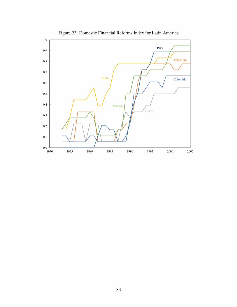
Figure 23: Domestic Financial Reforms Index for Latin America

0.0

0.1

0.2

0.3

0.4

0.5

0.6

0.7

0.8

0.9

1.0

1970 1975 1980 1985 1990 1995 2000 2005

Mexico

Colombia

Brazil

Chile

Argentina

Peru

83

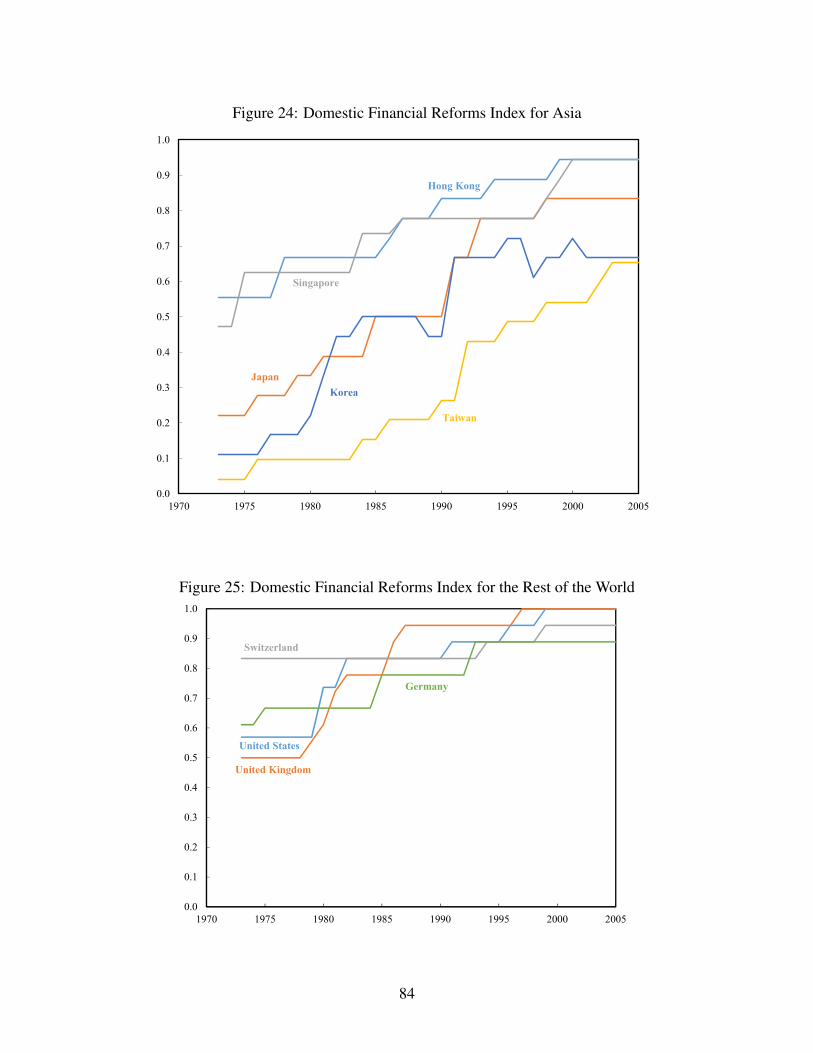
Figure 24: Domestic Financial Reforms Index for Asia

0.0

0.1

0.2

0.3

0.4

0.5

0.6

0.7

0.8

0.9

1.0

1970 1975 1980 1985 1990 1995 2000 2005

Taiwan

KoreaJapan

Singapore

Hong Kong

Figure 25: Domestic Financial Reforms Index for the Rest of the World

0.0

0.1

0.2

0.3

0.4

0.5

0.6

0.7

0.8

0.9

1.0

1970 1975 1980 1985 1990 1995 2000 2005

Switzerland

United Kingdom

United States

Germany

84

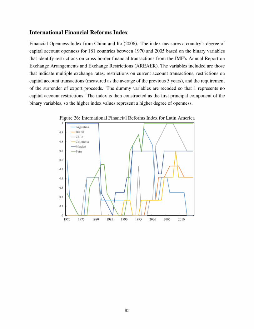
International Financial Reforms Index

Financial Openness Index from Chinn and Ito (2006). The index measures a country’s degree ofcapital account openness for 181 countries between 1970 and 2005 based on the binary variablesthat identify restrictions on cross-border financial transactions from the IMF’s Annual Report onExchange Arrangements and Exchange Restrictions (AREAER). The variables included are thosethat indicate multiple exchange rates, restrictions on current account transactions, restrictions oncapital account transactions (measured as the average of the previous 5 years), and the requirementof the surrender of export proceeds. The dummy variables are recoded so that 1 represents nocapital account restrictions. The index is then constructed as the first principal component of thebinary variables, so the higher index values represent a higher degree of openness.

Figure 26: International Financial Reforms Index for Latin America

0

0.1

0.2

0.3

0.4

0.5

0.6

0.7

0.8

0.9

1

1970 1975 1980 1985 1990 1995 2000 2005 2010

ArgentinaBrazilChileColombiaMexicoPeru

85

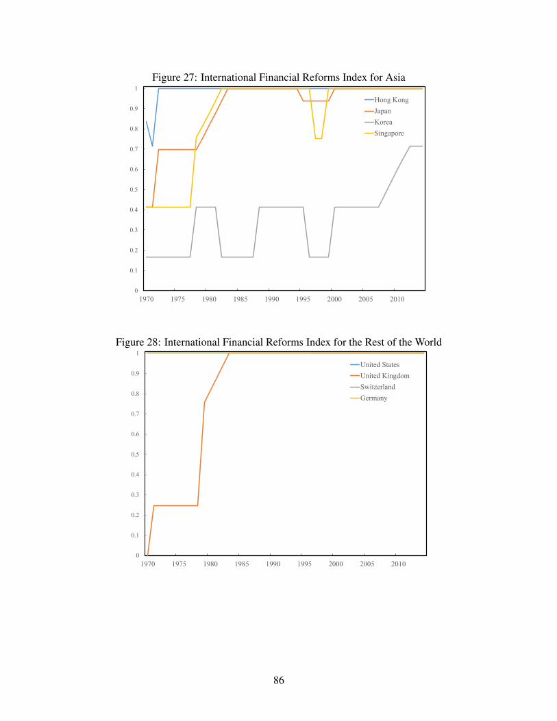
Figure 27: International Financial Reforms Index for Asia

0

0.1

0.2

0.3

0.4

0.5

0.6

0.7

0.8

0.9

1

1970 1975 1980 1985 1990 1995 2000 2005 2010

Hong KongJapanKoreaSingapore

Figure 28: International Financial Reforms Index for the Rest of the World

0

0.1

0.2

0.3

0.4

0.5

0.6

0.7

0.8

0.9

1

1970 1975 1980 1985 1990 1995 2000 2005 2010

United StatesUnited KingdomSwitzerlandGermany

86

Appendix E: More on Robustness and Extensions

Functional Forms and Parameter Values

Above we wrote down a benchmark model against which the data could be compared with a viewto identifying wedges between what the model predicts and what the data show. As is conventional,and for concreteness, we interpreted these wedges as taxes and subsidies that affect the marginal op-timality conditions of firms and households. In discussing our results, we compared our estimatedwedges with both qualitative and quantitative indicators of taxes and factor market distortions andargued that the results were similar. That is, the interpretation of these wedges as a combinationsof taxes and subsidies and no-tax distortions was reasonable.

Nonetheless, any differences between our benchmark model and the “true model” of the datagenerating process will also show up as wedges. One possible cause of misspecification arises fromspecific parameter choices that were calibrated ex ante, as opposed to being estimated from the data.This includes the levels of some parameters which might be viewed as controversial, as well as theassumption that the key parameters describing production and preferences across countries are thesame across countries and over time. In this subsection, we illustrate how alternative assumptionsabout parameter values affect the identified wedges and the resulting analysis.

To preview our results, we show that, for two such parameters—the discount factor b and thepreference for leisure parameter y—changing their values or allowing variation across countrieshas no effect on our results, as they serve only to scale up or down the average level of the laborand capital wedges. That is, they affect the level of the estimated wedges, but not their relativemovements over time. Although the remaining calibrated parameters could conceivably play amore significant role, we show that our results vary little when two of these parameters—the outputelasticity of capital a and the size of adjustment costs parameter n—are varied within the range ofestimates available in the literature.

The Discount Factor b and Preference for Leisure y

Rearranging the optimality conditions of the household and firms yields

1� thjt =

y1�a

hg+1jt

Cjt

Yjt,

which shows that, given data for country j at time t on hours h jt , consumption Cjt and output Yjt ,and given the Frisch elasticity of labor supply parameter g, we can pin down the product of thelabor wedge with the output elasticity of labor parameter a divided by the parameter governing thevalue of leisure y. This means that we cannot separately identify the level of the labor wedge from

87

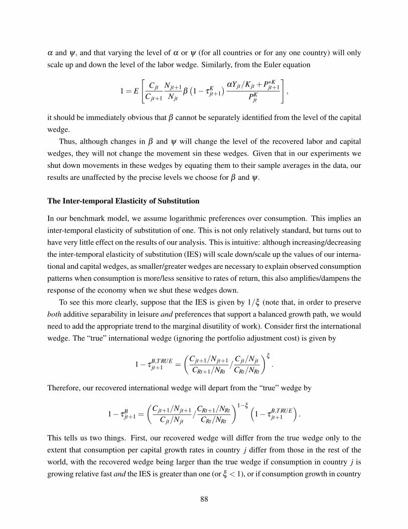
a and y, and that varying the level of a or y (for all countries or for any one country) will onlyscale up and down the level of the labor wedge. Similarly, from the Euler equation

1 = E

"Cjt

Cjt+1

Njt+1

Njtb�1� tK

jt+1� aYjt/Kjt +P⇤K

jt+1

PKjt

#,

it should be immediately obvious that b cannot be separately identified from the level of the capitalwedge.

Thus, although changes in b and y will change the level of the recovered labor and capitalwedges, they will not change the movement sin these wedges. Given that in our experiments weshut down movements in these wedges by equating them to their sample averages in the data, ourresults are unaffected by the precise levels we choose for b and y.

The Inter-temporal Elasticity of Substitution

In our benchmark model, we assume logarithmic preferences over consumption. This implies aninter-temporal elasticity of substitution of one. This is not only relatively standard, but turns out tohave very little effect on the results of our analysis. This is intuitive: although increasing/decreasingthe inter-temporal elasticity of substitution (IES) will scale down/scale up the values of our interna-tional and capital wedges, as smaller/greater wedges are necessary to explain observed consumptionpatterns when consumption is more/less sensitive to rates of return, this also amplifies/dampens theresponse of the economy when we shut these wedges down.

To see this more clearly, suppose that the IES is given by 1/x (note that, in order to preserveboth additive separability in leisure and preferences that support a balanced growth path, we wouldneed to add the appropriate trend to the marginal disutility of work). Consider first the internationalwedge. The “true” international wedge (ignoring the portfolio adjustment cost) is given by

1� tB,T RUEjt+1 =

✓Cjt+1/Njt+1

CRt+1/NRt/

Cjt/Njt

CRt/NRt

◆x.

Therefore, our recovered international wedge will depart from the “true” wedge by

1� tBjt+1 =

✓Cjt+1/Njt+1

Cjt/Njt/

CRt+1/NRt

CRt/NRt

◆1�x ⇣1� tB,T RUE

jt+1

⌘.

This tells us two things. First, our recovered wedge will differ from the true wedge only to theextent that consumption per capital growth rates in country j differ from those in the rest of theworld, with the recovered wedge being larger than the true wedge if consumption in country j isgrowing relative fast and the IES is greater than one (or x < 1), or if consumption growth in country

88

j is relative slow and the ISE is greater than one. This is intuitive; if consumption in country j isgrowing relatively fast, it must be because the country perceives a relatively higher return to foreigninvestments. The smaller is the IES, the greater is the wedge required to induce faster consumptiongrowth. Second, when we do experiments in which we shut this wedge down, we are also shuttingthe true wedge down. That is, when we assess the importance of the wedge, we are generatingthe same behavior for relative consumption growth in country j, regardless of whether we haveidentified the true wedge of nor. Of course, the behavior of other countries may still differ.

Now consider the capital wedge under the same assumption. The “true” capital wedge satisfies

1 = E

"✓Cjt/Njt

Cjt+1/Njt+1

◆xb⇣

1� tK,T RUEjt+1

⌘ aYjt/Kjt +P⇤Kjt+1

PKjt

#,

and hence, everything else equal, our recovered wedge departs from the “true wedge” by

1� tKjt+1 =

✓Cjt+1/Njt+1

Cjt/Njt

◆1�x ⇣1� tK,T RUE

jt+1

⌘.

The findings are similar to those for the international wedge, except now we refer to the absolutegrowth rate of consumption rather than the relative growth rate. That is, the wedges are scalingsthat depend on the growth rate of consumption and the size of the IES, and that shutting down therecovered wedge is equivalent to shutting down the true wedge.

However, unlike with the international wedge where consumption per capita growth was data,the calculation of the capital wedge requires estimating a capital stock. Hence, it is possible thatour procedure will return different capital stocks and hence wedges that are not simply scaled inthis fashion. However, in practice, this does not appear to be the case. Moreover, experiments withdifferent assumptions on the IES reveal almost identical results.

The Output Elasticity of Capital a

One parameter that has been the subject of a great deal of attention in the literature is the outputelasticity of capital parameter a which, in a frictionless world, also parameterizes the capital share.Not only do measured capital shares vary across countries, but there has been a substantial debateas to whether they accurately capture the division of factor payments between labor and capital(for example, Gollin 2002), and whether they are miss-measured due to the inclusion of returns tonon-reproducible factors such as land in returns to capital (for example, Caselli and Feyrer (2007)).There is also a significant literature looking at trends in the capital share over time that questionswhether a Cobb-Douglas production function is a good representation of production possibilities inthe economy (for example, Karabarbounis and Neiman (2014)). In what follows, we address each

89

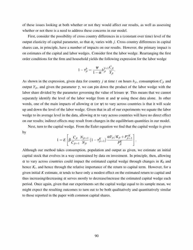
of these issues looking at both whether or not they would affect our results, as well as assessingwhether or not there is a need to address these concerns in our model.

First, consider the possibility of cross country differences in a (constant over time) level of theoutput elasticity of capital parameter, so that a j varies with j. Cross country differences in capitalshares can, in principle, have a number of impacts on our results. However, the primary impact ison estimates of the capital and labor wedges. Consider first the labor wedge. Rearranging the firstorder conditions for the firm and household yields the following expression for the labor wedge

1� thjt =

y1�a

hg+1jt

Cjt

Yjt.

As shown in the expression, given data for country j at time t on hours h jt , consumption Cjt andoutput Yjt , and given the parameter g, we can pin down the product of the labor wedge with thelabor share divided by the parameter governing the value of leisure y. This means that we cannotseparately identify the level of the labor wedge from a and y using these data alone. In otherwords, one of the main impacts of allowing a (or y) to vary across countries is that it will scaleup and down the level of the labor wedge. Given that in all of our experiments we equate the laborwedge to its average level in the data, allowing a to vary across countries will have no direct effecton our results; indirect effects may result from changes in the equilibrium quantities in our model.

Next, turn to the capital wedge. From the Euler equation we find that the capital wedge is givenby

1 = E

"b

Cjt

Cjt+1

Njt+1

Njt

�1� tK

jt+1� aYjt/Kjt +P⇤K

jt+1

PKjt

#.

Although our method takes consumption, population and output as given, we estimate an initialcapital stock that evolves in a way constrained by data on investment. In principle, then, allowinga to vary across countries could impact the estimated capital wedge through changes in K0 andhence Kt , and hence through the relative importance of the return to capital term. However, for agiven initial K estimate, a tends to have only a modest effect on the estimated return to capital andthus increasing/decreasing a serves mostly to decrease/increase the estimated capital wedge eachperiod. Once again, given that our experiments set the capital wedge equal to its sample mean, wemight expect the resulting outcomes to turn out to be both qualitatively and quantitatively similarto those reported in the paper with common capital shares.

90

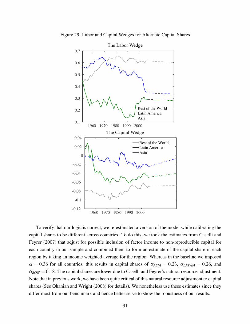
Figure 29: Labor and Capital Wedges for Alternate Capital Shares

The Labor Wedge

1960 1970 1980 1990 20000.1

0.2

0.3

0.4

0.5

0.6

0.7

Rest of the WorldLatin AmericaAsia

The Capital Wedge

1960 1970 1980 1990 2000-0.12

-0.1

-0.08

-0.06

-0.04

-0.02

0

0.02

0.04Rest of the WorldLatin AmericaAsia

To verify that our logic is correct, we re-estimated a version of the model while calibrating thecapital shares to be different across countries. To do this, we took the estimates from Caselli andFeyrer (2007) that adjust for possible inclusion of factor income to non-reproducible capital foreach country in our sample and combined them to form an estimate of the capital share in eachregion by taking an income weighted average for the region. Whereas in the baseline we imposeda = 0.36 for all countries, this results in capital shares of aASIA = 0.23, aLATAM = 0.26, andaROW = 0.18. The capital shares are lower due to Caselli and Feyrer’s natural resource adjustment.Note that in previous work, we have been quite critical of this natural resource adjustment to capitalshares (See Ohanian and Wright (2008) for details). We nonetheless use these estimates since theydiffer most from our benchmark and hence better serve to show the robustness of our results.

91

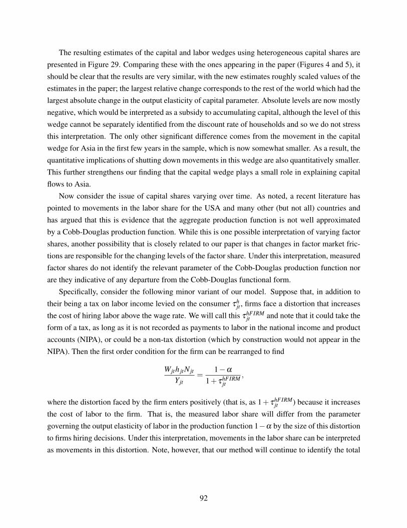
The resulting estimates of the capital and labor wedges using heterogeneous capital shares arepresented in Figure 29. Comparing these with the ones appearing in the paper (Figures 4 and 5), itshould be clear that the results are very similar, with the new estimates roughly scaled values of theestimates in the paper; the largest relative change corresponds to the rest of the world which had thelargest absolute change in the output elasticity of capital parameter. Absolute levels are now mostlynegative, which would be interpreted as a subsidy to accumulating capital, although the level of thiswedge cannot be separately identified from the discount rate of households and so we do not stressthis interpretation. The only other significant difference comes from the movement in the capitalwedge for Asia in the first few years in the sample, which is now somewhat smaller. As a result, thequantitative implications of shutting down movements in this wedge are also quantitatively smaller.This further strengthens our finding that the capital wedge plays a small role in explaining capitalflows to Asia.

Now consider the issue of capital shares varying over time. As noted, a recent literature haspointed to movements in the labor share for the USA and many other (but not all) countries andhas argued that this is evidence that the aggregate production function is not well approximatedby a Cobb-Douglas production function. While this is one possible interpretation of varying factorshares, another possibility that is closely related to our paper is that changes in factor market fric-tions are responsible for the changing levels of the factor share. Under this interpretation, measuredfactor shares do not identify the relevant parameter of the Cobb-Douglas production function norare they indicative of any departure from the Cobb-Douglas functional form.

Specifically, consider the following minor variant of our model. Suppose that, in addition totheir being a tax on labor income levied on the consumer th

jt , firms face a distortion that increasesthe cost of hiring labor above the wage rate. We will call this thFIRM

jt and note that it could take theform of a tax, as long as it is not recorded as payments to labor in the national income and productaccounts (NIPA), or could be a non-tax distortion (which by construction would not appear in theNIPA). Then the first order condition for the firm can be rearranged to find

Wjth jtNjt

Yjt=

1�a1+ thFIRM

jt,

where the distortion faced by the firm enters positively (that is, as 1+ thFIRMjt ) because it increases

the cost of labor to the firm. That is, the measured labor share will differ from the parametergoverning the output elasticity of labor in the production function 1�a by the size of this distortionto firms hiring decisions. Under this interpretation, movements in the labor share can be interpretedas movements in this distortion. Note, however, that our method will continue to identify the total

92

wedge on labor, calculated in this modified version as

1� thjt

1+ thFIRMjt

=y

1�ahg+1

jtCjt

Yjt.

In other words, the usual tax incidence result holds. Note also that it is worth pointing out that,returning to our first point, differences in the level of factor market frictions across countries couldalso explain recorded differences in the level of capital shares across countries, and not just timeseries variation in factor shares.

In light of these issues, and given that the Cobb-Douglas assumption remains relatively standardin many models, we retain the Cobb-Douglas assumption and note that our recovered wedges couldform the basis of a promising research agenda in which data on our labor wedge, along with dataon the changing labor share, can be used to separately identify changes in labor market distortionsthat are priced into wages, and those that are not.

The Adjustment Cost Parameter n

It has long been recognized that adjustment costs play an important role in helping international realbusiness cycle models more closely match the data on investment fluctuations in open economies(Baxter and Crucini (1993)). However, in calibrated versions of these models, there has beenlittle agreement as to how best to calibrate the parameters of the adjustment cost function. Inthis subsection, we review the issues, especially as applied to data on emerging market countries,describe our calibration strategy, and report sensitivity results for a different calibration.

As is traditional, we parameterize the adjustment cost of capital reference level k so that ad-justment costs are zero in the deterministic steady state. This also implies that average Tobin’s q isone in the deterministic steady state. To parameterize adjustment costs outside of steady state, wefollow Bernanke, Gertler, and Gilchrist (1999), Chari, Kehoe and McGrattan (2007) and others bysetting the scale parameter n to deliver a specific elasticity of the price of capital with respect tothe investment-capital ratio. Noting that

d logPKjt

d log�Xjty/Kjt

� =f 00⇣

XjtKjt

⌘XjtKjt

1�f 0⇣

XjtKjt

⌘ ,

and imposing the fact that under our assumptions on f , in steady state

f✓

Xjt

Kjt

◆= f 0

✓Xjt

Kjt

◆= 0,

93

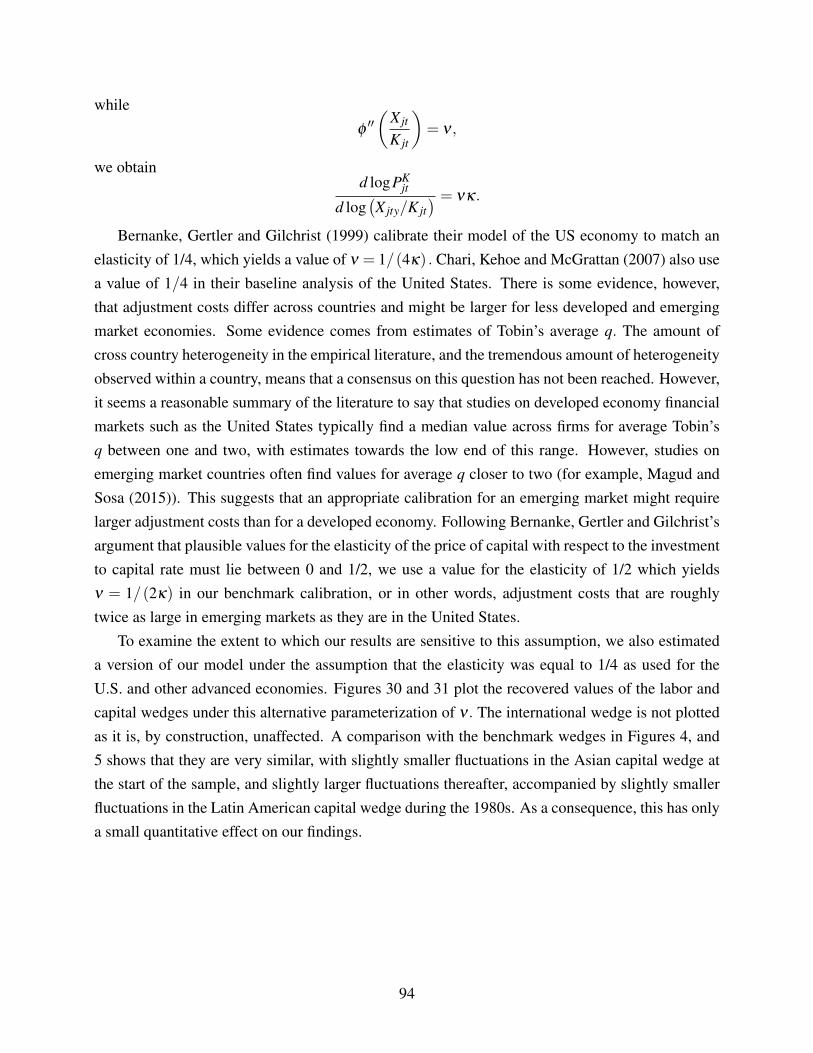
whilef 00✓

Xjt

Kjt

◆= n ,

we obtaind logPK

jt

d log�Xjty/Kjt

� = nk.

Bernanke, Gertler and Gilchrist (1999) calibrate their model of the US economy to match anelasticity of 1/4, which yields a value of n = 1/(4k) . Chari, Kehoe and McGrattan (2007) also usea value of 1/4 in their baseline analysis of the United States. There is some evidence, however,that adjustment costs differ across countries and might be larger for less developed and emergingmarket economies. Some evidence comes from estimates of Tobin’s average q. The amount ofcross country heterogeneity in the empirical literature, and the tremendous amount of heterogeneityobserved within a country, means that a consensus on this question has not been reached. However,it seems a reasonable summary of the literature to say that studies on developed economy financialmarkets such as the United States typically find a median value across firms for average Tobin’sq between one and two, with estimates towards the low end of this range. However, studies onemerging market countries often find values for average q closer to two (for example, Magud andSosa (2015)). This suggests that an appropriate calibration for an emerging market might requirelarger adjustment costs than for a developed economy. Following Bernanke, Gertler and Gilchrist’sargument that plausible values for the elasticity of the price of capital with respect to the investmentto capital rate must lie between 0 and 1/2, we use a value for the elasticity of 1/2 which yieldsn = 1/(2k) in our benchmark calibration, or in other words, adjustment costs that are roughlytwice as large in emerging markets as they are in the United States.

To examine the extent to which our results are sensitive to this assumption, we also estimateda version of our model under the assumption that the elasticity was equal to 1/4 as used for theU.S. and other advanced economies. Figures 30 and 31 plot the recovered values of the labor andcapital wedges under this alternative parameterization of n . The international wedge is not plottedas it is, by construction, unaffected. A comparison with the benchmark wedges in Figures 4, and5 shows that they are very similar, with slightly smaller fluctuations in the Asian capital wedge atthe start of the sample, and slightly larger fluctuations thereafter, accompanied by slightly smallerfluctuations in the Latin American capital wedge during the 1980s. As a consequence, this has onlya small quantitative effect on our findings.

94

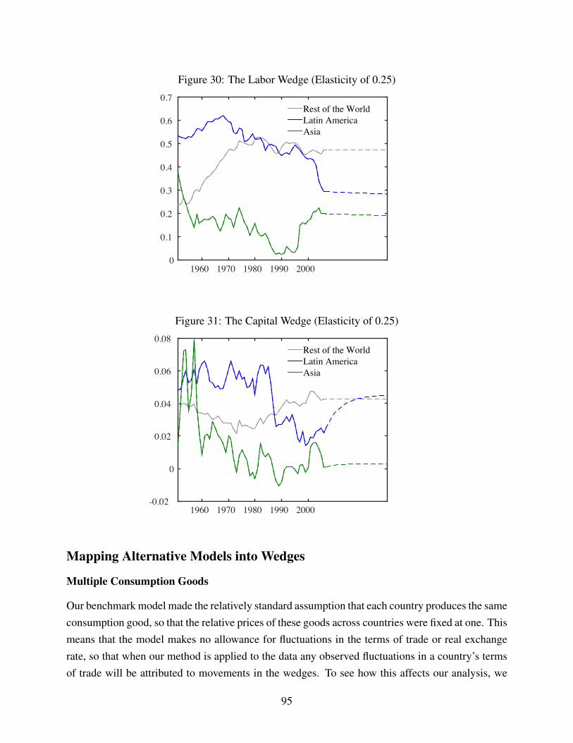
Figure 30: The Labor Wedge (Elasticity of 0.25)

1960 1970 1980 1990 20000

0.1

0.2

0.3

0.4

0.5

0.6

0.7Rest of the WorldLatin AmericaAsia

Figure 31: The Capital Wedge (Elasticity of 0.25)

1960 1970 1980 1990 2000-0.02

0

0.02

0.04

0.06

0.08Rest of the WorldLatin AmericaAsia

Mapping Alternative Models into Wedges

Multiple Consumption Goods

Our benchmark model made the relatively standard assumption that each country produces the sameconsumption good, so that the relative prices of these goods across countries were fixed at one. Thismeans that the model makes no allowance for fluctuations in the terms of trade or real exchangerate, so that when our method is applied to the data any observed fluctuations in a country’s termsof trade will be attributed to movements in the wedges. To see how this affects our analysis, we

95

consider a simple multi-good international real business cycle model along the lines of Backus,Kehoe, and Kydland (1994) adapted to our framework.

Specifically, consider a version of the world economy in our benchmark in which there are only2 countries (which allows for a simpler representation of relative prices), the population is fixedat one in each country in all periods, there is no government, and there are no adjustment costs.Preferences are given by

E0

"•

Ât=0

b t⇢

lnCjt �y

1+ gH1+g

jt

�#,

where consumption is of a non-traded aggregate good that is described below. The budget constraintfor households in each region is given by

Pjt�Cjt +Kjt+1 � (1�d )Kjt

�+Et

⇥qt+1B jt+1

⇤WjtHjt ++rK

jtKjt +B jt ,

where the bond is the numeraire, and Pjt is the price of the non-traded aggregate good specific tocountry j that can be used for both consumption and investment. The wages and rental rates ofcapital paid by the firms that produce the domestic tradable good are also expressed in terms of thenumeraire. The FONCs of the households problem include

b t 1Cjt

= l jtPjt ,

b tyHgjt = l jtWjt ,

l jtPjt = Et⇥l jt+1

�rK

jt+1 �Pjt+1 (1�d )�⇤

qt+1l jt = l jt+1.

There are two types of firms in the economy. The first produces the domestic tradable good andmaximizes profits

p jtA jtKajt�h jtNjt

�1�a �WjtHjt � rKjtKjt ,

where p jt is the price of the j0th country’s tradable good. This problem yields optimality conditions

p jtaYjt

Kjt= rK

jt ,

p jt (1�a)Yjt

Hjt= Wjt .

The second type of firm produces the domestic non-tradable good using both the domestic andforeign tradable goods. They maximize profits

PjtG j⇣

Y j1t ,Y

j2t

⌘� p1tY

j1t � p2tY

j2t ,

96

where the production function G j is country specific and takes the constant elasticity of substitutionform

G j⇣

Y j1t ,Y

j2t

⌘=

✓c⇣

Y jjt

⌘(s�1)/s+(1�c)

⇣Y j� jt

⌘(s�1)/s◆s/(s�1)

,

where � j denotes the country that is “not j.” We will assume that the elasticity of substitution isno greater than one so that both goods are necessary for production and hence we do not have toworry about a corner in which one country’s exports are zero. Competition ensures that the priceof the non-tradable is given by

Pjt =⇣

c p1�sjt +(1�c) p1�s

� jt

⌘1/(1�s).

The optimality conditions of the household can then be combined with these results on equilib-rium prices to deduce the implications of the model for our recovered wedges. Specifically, assumethat our procedure was applied to data generated by this model with multiple consumption goods.Then the optimal choice of leisure satisfies

yHgjt =

1PjtCjt

p jt (1�a)Yjt

Hjt,

so that the recovered labor wedge satisfies

1� thjt =

y1�a

Hgjt

Hjt

YjtCjt

=p jt

Pjt=

c +(1�c)

✓p� jt

p jt

◆1�s!�1/(1�s)

=⇣

c +(1�c)�TOTjt

��(1�s)⌘�1/(1�s)

,

a positive function of country j0s terms of trade TOTjt = p jt/p� jt . That is, if the terms of tradedeteriorates, the labor wedge th rises. Why? If the price of the foreign good rises, while the priceof the domestic good is unchanged, the price index for consumers goes up and labor supply falls forthe given price of the country’s output. To put it differently, the real wage received by the supplierof labor differs from the real cost of labor to the firm, because they face different prices. Thus, adeterioration in a country’s terms of trade acts like an increase in the labor wedge.

The optimal choice of capital satisfies

1 = bEt

Cjt

Cjt+1

1Pjt

✓p jta

Yjt

Kjt�Pjt+1 (1�d )

◆�

97

= bEt

2

4 Cjt

Cjt+1

⇣p jt

Pjt+1

⌘a Yjt

Kjt� (1�d )

a YjtKjt

� (1�d )

✓a

Yjt

Kjt� (1�d )

◆3

5 ,

so that the capital wedge is given by

1� tKjt =

p jtPjt

a YjtKjt

� (1�d )

a YjtKjt

� (1�d ),

and, once again, a deterioration in the terms of trade increases the capital wedge and causes thecapital and labor wedges to comove positively.

Lastly, the optimality condition for bonds yields

qt+1 = bPjtCjt

Pjt+1Cjt+1,

orCjt+1

Cjt= b 1+ rt+1

Pjt+1/Pjt,

where1+ rt+1 = 1/qt+1,

for all j. That is, the real interest rate in country j departs from the world interest rate rt+1 by thecountry specific rate of inflation.

Hence, the international wedge is given by differences in country specific rates of inflationwhich, in this two good two country world, are determined by fluctuations in the terms of trade. Tosee this, note that our method recovers

tBjt+1 = 1�

Cjt+1/Cjt

C� jt+1/C� jt

= 1�Pjt/Pjt+1

P� jt/P� jt+1

= 1�

0

@

⇣c p1�s

jt +(1�c) p1�s� jt

⌘/⇣

c p1�sjt+1 +(1�c) p1�s

� jt+1

⌘

⇣(1�c) p1�s

jt +c p1�s� jt

⌘/⇣(1�c) p1�s

jt+1 +c p1�s� jt+1

⌘

1

A1/(1�s)

= 1�

0

@

⇣c�TOTjt

�1�s+(1�c)

⌘/⇣

c�TOTjt+1

�1�s+(1�c)1�s

⌘

⇣(1�c)

�TOTjt

�1�s+c⌘/⇣(1�c)

�TOTjt+1

�1�s+c1�s

⌘

1

A1/(1�s)

.

Regarding production and productivity, movements in the terms of trade plays no role in mea-sured outcomes. This is easiest to see if we consider the incomes method for computing nominal

98

gross domestic product which yields, in terms of the numeraire

GDPjt =WjtHjt ++rKjtKjt = p jtA jtKa

jt�h jtNjt

�1�a.

Holding prices constant in some base year T, real GDP in period t is then given by

GDPTjt = p jT A jtKa

jt�h jtNjt

�1�a,

so that measured productivity growth is unaffected by movements in the terms of trade. Thus, in thecontext of this model, terms of trade fluctuations imply no specific pattern of correlation betweenour recovered wedges and productivity.

In summary, this model implies that the labor and capital wedges should comove with the termsof trade of a country, while the international wedge will in general move (positively or negatively)with the change in the terms of trade. Note that, if c = 1/2, the international wedge is always zero.As our recovered wedges show only modest comovement with each other, we conclude that thismodel is not especially promising as an explanation for the patterns we observe.

However, an alternative specification with multiple consumption goods, and possibly the addi-tion of transport costs along the lines of Obstfeld and Rogoff (2001), may contribute towards anexplanation of our findings. We consider this next.

Transport Costs

Obstfeld and Rogoff (2001) and others have argued that the addition of transport costs in inter-national goods trade may help explain patterns in international capital flows. To understand thisargument, note that trade costs—modeled as iceberg costs—serve primarily to influence the termsof trade by driving a wedge between the domestic and foreign price of a given good. Specifically,in the model of the previous subsection—where each country produces and exports its own goodin all periods—trade costs of size t on all goods imply the following relationship between relativeprices of the same good across countries

p j� jt =

p� j� jt

1� t,

p jjt = (1� t) p� j

jt ,

where pijt denotes the price in country i of the good produced by country j at time t. Note that

our expressions for the capital and labor wedges are unchanged, although in the background the

99

transport costs affects both the level of the terms of trade, and its relationship across countries

TOTjt =p j

jt

p j� jt

= (1� t)2 p� jjt

p� j� jt

=(1� t)2

TOT� jt.

Transport costs play a more obvious role in the international wedge as

Pjt

Pjt+1=

0

B@c⇣

p jjt

⌘1�s+(1�c)

⇣p j� jt

⌘1�s

c⇣

p jjt+1

⌘1�s+(1�c)

⇣p j� jt+1

⌘1�s

1

CA

1/(1�s)

=p j� jt

p j� jt+1

c�TOTjt

�1�s+(1�c)

c�TOTjt+1

�1�s+(1�c)

!1/(1�s)

,

P� jt

P� jt+1=

0

B@(1�c)

⇣p� j

jt

⌘1�s+c

⇣p� j� jt

⌘1�s

(1�c)⇣

p� jjt+1

⌘1�s+c

⇣p� j� jt+1

⌘1�s

1

CA

1/(1�s)

=p� j� jt

p� j� jt+1

0

B@(1�c)

⇣TOTjt

(1�t)2

⌘1�s+c

(1�c)⇣

TOTjt+1

(1�t)2

⌘1�s+c

1

CA

1/(1�s)

,

so that

tBjt+1 = 1�

Pjt/Pjt+1

P� jt/P� jt+1

= 1�

p j� jt

p j� jt+1

✓c(TOTjt)

1�s+(1�c)

c(TOTjt+1)1�s

+(1�c)

◆1/(1�s)

p� j� jt

p� j� jt+1

✓(1�c)(TOTjt)

1�s+c(1�t)2(1�s)

(1�c)(TOTjt+1)1�s

+c(1�t)2(1�s)

◆1/(1�s)

= 1�

✓c(TOTjt)

1�s+(1�c)

c(TOTjt+1)1�s

+(1�c)

◆1/(1�s)

✓(1�c)(TOTjt)

1�s+c(1�t)2(1�s)

(1�c)(TOTjt+1)1�s

+c(1�t)2(1�s)

◆1/(1�s).

That is, with constant t over time, transport costs further the difference in c.Many authors have argued that transport costs have declined over time and have played a causal

role in the expansion of global trade. To see the effect of this, consider a version of the above worldin which one country is small and so takes world prices as given. We denote world prices by anasterisk, and index t by time, while still maintaining the assumption that both goods attract the

100

same transport costs. Then substituting into the above formulae the fact that the terms of trade ofthis small country, given a (assumed constant) world relative price of goods

TOTjt = (1� tt)2 p⇤jt

p⇤� jt.

With world relative prices fixed, this small country should then have experienced an increase inits terms of trade over time. Given the results above, this implies that our recovered labor andcapital wedges should both display downward trends over time. Although we find some evidencefor downward trends in our results above, it is possible that these trends were driven by otherfactors such as the tendency to liberalize factor markets over time. More work will be requiredto distinguish the effect of trade costs from the effect of other changes in these economies. Overshorter horizons, the absence of a significant correlation between our measures suggests that thismechanism is less important.

Lastly, in the above we have assumed that each country produces its own distinct good andexports it in all periods. Suppose that this is not true, and further, suppose that our small openeconomy is a net importer and borrower in one period. In a finite horizon economy, it is necessarilythe case that, in some future period, the country must become a net exporter to pay off this borrow-ing. If this does not affect the identity of who exports which good, this has no additional effect towhat we have identified above. If however, in order to pay off its borrowing a country must switchfrom importing a good to exporting that same good, Obstfeld and Rogoff (2001) have shown thatthis can lead to movements in relative prices that deter capital flows.

To see this, note that if a small country imports the foreign good � j at time t then the price itpays is given by

p j� jt =

p⇤� jt

1� t,

as above. However, if at some later date s > t it switches to exporting that good, the price it receivesis given by

p j� js = (1� t) p⇤� jt .

If we, for simplicity, assume that world prices are constant over time, then this implies that

Pjt

Pjs=

0

B@c⇣(1� t) p⇤j

⌘1�s+(1�c)

⇣ p⇤� j1�t

⌘1�s

c⇣(1� t) p⇤j

⌘1�s+(1�c)

⇣(1� t) p⇤� j

⌘1�s

1

CA

1/(1�s)

=

0

B@c⇣

p⇤j⌘1�s

+(1�c)⇣ p⇤� j

(1�t)2

⌘1�s

c⇣

p⇤j⌘1�s

+(1�c)⇣

p⇤� j

⌘1�s

1

CA

1/(1�s)

> 1,

101

so that there is deflation between periods t and s. But this implies that the real interest rate facedby borrowers in the country over this time horizon is larger than the real interest rate available inworld markets. Likewise, a country that saves will eventually be repaid and the same mechanismwill operate in reverse.

In terms of the international wedge (against the rest of the world where, for simplicity, priceswere assumed constant), if the switch between importing and exporting the good occurred betweenperiods t and t +1, we would recover

tBjt+1 = 1�

Pjt/Pjt+1

PRt/PRt+1= 1�Pjt/Pjt+1,

which, for a country that imported in period t and exported in period t + 1, is greater than oneimplying a tax on foreign borrowing.

As this mechanism requires that a country switch from importing to exporting a set of goods,it is not clear that this mechanism should generate quantitatively significant effects on the levelof capital flows in practice. Nonetheless, we note that Reyes-Heroles (2016), Alessandria andChoi (2015), and Eaton, Kortum, and Neiman (2016) all find that trade costs play significant (butquantitatively varying) roles in explaining the level of capital flows in the context of their ownmodels. For this mechanism to explain the relative pattern of capital flows to Asia and LatinAmerica in the 1950s and 1960s, Asia must have expected a large number of goods to switch frombeing imported to being exported in order to significantly deter capital flows, while the switchesin Latin America would have been expected to be smaller. To fully investigate this possibilitywould require a detailed examination of international trade at a commodity level which would be aworthwhile subject for a future paper.

Capacity Utilization

In the text, we completely abstracted from the possibility of fluctuations in capacity utilization. Thiswas deliberate as fluctuations in capacity utilization tend to occur at business cycle frequencies,and hence did not seem to be especially important in driving the medium term movements infundamentals that primarily determine capital flows. Nonetheless, we quickly review the issuesin this section.

One possible way to incorporate variable capacity utilization into a business cycle accountingframework was explored in Chari, Kehoe, and McGrattan (2007) who consider a variable workweekalong the lines of that studied in Hornstein and Prescott (1993). They show that, when introducedin this way, variable capacity utilization generates measured labor wedges and productivity (theyrefer to productivity as the efficiency wedge) that are negatively correlated, without generating a

102

capital wedge. Adapted to an open economy, this will not affect our international wedge.In this section, we consider an alternate variant, designed for our open economy framework,

in which capital utilization requires the use of an important input which we refer to as energy andwhich we think of as representing imported oil. As above, we assume that the population is fixedat one in every country and that there is no government or adjustment costs in capital. Suppose thatcapital services are produced using physical capital and energy

KS jt = KfjtE

1�fjt ,

and that

Yjt = A jt�KS jt

�a H1�ajt

= A jtKafjt Ea(1�f)

jt H1�ajt .

This framework bears a resemblance to the set-up in Backus and Crucini (2000). Unlike thatpaper, we will interpret increases in energy expenditures per unit capital as representing increasesin capacity utilization which come at the cost of increasing the rate of depreciation of capital, sothat

Kjt+1 =

✓1�d

✓E jt

Kjt

◆◆Kjt +Xjt .

With a little bit of work, it can be shown that the Euler equation for the household in capital isgiven by

1 = Et

b

Cjt

Cjt+1

✓fa

Yjt

Kjt+1�d

✓E jt

Kjt

◆+d 0

✓E jt

Kjt

◆E jt

Kjt

◆�,

so that, if we apply our methodology using a fixed depreciation rate of d�E j/Kj

�calculated at the

balanced growth path level of energy use per unit of capital E j/Kj we obtain a capital wedge

1� tKjt =

fa YjtKjt

+1�d⇣

E jtKjt

⌘+d 0

⇣E jtKjt

⌘E jtKjt

fa YjtKjt

+1�d⇣

E jssKjss

⌘ .

Now, suppose we are in the vicinity of the average level of energy usage per unit capital, andfurther suppose that an increase in the price of oil causes energy per unit capital to fall. Thendepreciation falls and the capital wedge falls. That is, there is a negative relationship between theprice of energy and the capital wedge.

103

Financial Frictions due to Limited Commitment

One model of international financial frictions that has attracted a great deal of attention positsthat international capital flows are constrained by the possibility that a country might choose to exitthe international financial system and stay in autarky. These limited commitment models have beenstudied by many authors including Wright (2001), Kehoe and Perri (2002) and Restrepo-Echavarria(2018).

In this subsection, we outline a variant of these models in an environment similar to the oneconsidered in our paper. For simplicity we assume that there are no adjustment costs of capital, nogovernment, and that the population of each country is fixed at one throughout time. Specifically,consider a social planner whose problem is to choose state, date and country contingent sequencesof consumption, capital, and hours worked to maximize

E0

"

Âj

cCjt

•

Ât=0

b t⇢

lnCjt �y

1+ gH1+g

jt

�#,

subject to a world resource constraint for each state and date,

Âj

�Cjt +Kjt+1 +G jt

= Â

jYjt = Â

j

nA jtKa

jt H1�ajt +(1�d )Kjt

o,

and a series of state and date contingent participation constraint for each country j of the form,

Et

"•

Ât=0

b t⇢

lnCjt �y

1+ gH1+g

jt

�#�V A

j�Kjt ,st

�,

where V Aj is the value to country j of exiting the international economy and staying in autarky

forever after, which depends on the amount of capital they would take with them and the currentstate of the world indexed by st (the expectation operator Et is an expectation conditioned on thisst).

If we let lt denote the multipliers on the world budget constraint at time t, and µ jt/b s themultipliers on the participation constraints of country j, the first order conditions for an optimumyield

b t

cC

jt +t

Âs=0

µ js

!1

Cjt= lt ,

b t

cC

jt +t

Âs=0

µ js

!yHg

jt = lt (1�a)Yjt

Hjt,

104

lt = Et

"lt+1

✓a

Yjt+1

Kjt+1+1�d

◆�µ jt+1

dV Aj�Kjt+1,st+1

�

dKjt+1

#.

If we let M�1 = cCjt and recursively define

Mjt = Mjt�1 +µ jt ,

then the first order conditions with respect to consumption for countries i and j will yield

Cjt

Cit=

Mjt

Mit. (27)

Note that Mjt can be thought of as a cumulative planner weight, which depends on the initial plan-ner weight assigned to each country and past Lagrange multipliers on the country’s participationconstraint which are positive only when the participation constraint binds.

Rearranging these equations and comparing them to the equations derived for our model it isstraightforward to show that the limited commitment model implies that there is no labor wedge

thjt = 1� y

1�aHg

jtHjt

YjtCjt = 0, (28)

and that the international wedge (relative to the rest of the world) is given by

tBjt+1 = 1�

Cjt+1/Cjt

CRt+1/CRt= 1�

Mjt+1/Mjt

MRt+1/MRt. (29)

As for the capital wedge, the Euler equation can be rearranged to yield

1 = bEt

"✓Mjt+1

Mjt

◆Cjt

Cjt+1

✓a

Yjt+1

Kjt+1+1�d

◆�µ jt+1

dV Aj�Kjt+1,st+1

�

dKjt+1

#

= bEt

"Cjt

Cjt+1

Mjt+1

Mjt�µ jt+1

Cjt+1

Cjt

1A jt+1aka�1

jt+1 +1�ddV A

j�Kjt+1,st+1

�

dKjt+1

!

⇥✓

aYjt+1

Kjt+1+1�d

◆�. (30)

Recall that the Euler equation derived in the paper, under the simplifying assumptions used here, isgiven by

1 = bEt

Cjt

Cjt+1

�1� tK

jt+1�✓

aYjt+1

Kjt+1+1�d

◆�. (31)

This means that the limited commitment model produces a capital wedge for the competitive equi-

105

librium formulation of the problem of

tKjt+1 = 1�

Mjt+1

Mjt�µ jt+1

Cjt+1

Cjt

1A jt+1aka�1

jt+1 +1�ddV A

j�Kjt+1,st+1

�

dKjt+1

!,

which will, in general, be highly correlated with the international wedge.Overall, the predictions of the limited commitment model are not borne out by the data on

capital flows. We find that there is a significant labor wedge, and that the correlation between theinternational and capital wedges is low.

Government Borrowing and Ricardian Equivalence

In our benchmark model, we assumed that the government in each region levied lump sum taxes(or made lump sum transfers) in order to ensure that the budget was balanced in each period.As a result, all capital flows were private in the sense of being owned or owed by households.This was without loss of generality in the theory because the model exhibited a form of RicardianEquivalence.

In practice, however, the distinction between private and public capital flows could be relevantin explaining the pattern of capital flows into Latin America, instead of into Asia, that we observe inthe first few decades of the post war period. Other authors have argued that this distinction mattersfor the later period when data on capital flows becomes more widely available. For example, bothAguiar and Amador (2016) and Alfaro, Kalemli-Ozcan and Volosovych (2014), have argued thatpublic capital flows—borrowing and saving by emerging market country governments—are thekey component in explaining capital flows beginning in the 1970s. It is also possible that similarforces were also relevant in the early decades that are our focus, although data limitations preventan extension of their analysis back to 1950. Implicitly, of course, this requires that there mustbe a significant departure from Ricardian Equivalence that prevents private capital flows (that is,flows to the private sector of these economies) from offsetting these public flows. In the modelof Amador and Aguiar (2016), for example, domestic voters are assumed to have no access tointernational capital markets and so Ricardian Equivalence does not hold. We are quite open tothis possibility and note that plausible reasons for the departure from Ricardian Equivalence havetestable implications that our wedges approach is well-designed to examine.

Specifically, one plausible hypothesis is that the capital controls that were introduced under theBretton-Woods system prevented the private sector from accessing international capital marketsto offset the effect of public capital flows. As noted, Aguiar and Amador (2016) impose this asan assumption in their model. But this implies that private consumption should depart from thelevels implied by the Euler equation for bonds which would show up as an international wedge in

106

our framework. The fact that we find that the international wedge has a relatively small impacton capital flows is evidence against this departure from Ricardian Equivalence being important inexplaining capital flows.

To see this, suppose to begin that households in Asia were limited in their ability to borrow asmuch as they would like. If borrowing constraints on Asian households were binding, the Eulerequation governing the household’s choice of foreign assets becomes (for j = A)

lAtqt+1 = b t+1z BAt+1 +lAt+1,

where z BAt+1 is the current value Lagrange multiplier on the constraint limiting borrowing (the

superscript B denotes a limit on borrowing) against income in the relevant state of the world inperiod t + 1. Our method would then use relative consumption per capita growth rates to recoverthe following wedge (under the assumption that the rest of the world is not borrowing constrained)

1� tBAt+1 =

CAt+1/NAt+1

CAt/NAt/

CRt+1/NRt+1

CRt/NRt= 1+z B

At+1.

That is, to explain the lack of capital flows into Asia, this departure from Ricardian Equivalencewould show up as a negative international wedge tB

jt+1. This is intuitive: If Asian households donot borrow, the method interprets this as a subsidy on savings or a tax on borrowing. Note also thatbinding borrowing constraints have no effect on the labor or capital wedges as we define them.

Now suppose that Latin American governments were borrowing in the 1950s and 1960s andthat Latin American households were limited in their ability to save so as to offset this borrowingas Ricardian equivalence would require. In this case, it is straightforward to show that the wedgerecovered for Latin America ( j = L) would be

1� tBLt+1 =

CLt+1/NLt+1

CLt/NLt/

CRt+1/NRt+1

CRt/NRt= 1�z S

Lt+1,

where z SLt+1 is now the current value multiplier on the binding constraint on international savings.

That is, we recover a tax on international savings in order to rationalize the relative lack of interna-tional savings by Latin American households.

In summary, if this departure from Ricardian equivalence is invoked to explain why privatesavings and borrowing behavior did not offset public borrowing in the first few decades of oursample, we should expect to see a large tax on international savings for Latin America, and asignificant subsidy on savings for Asia. Our recovered wedges provide only partial support for thishypothesis. On the one hand, we do find a significant subsidy—averaging around 5% during the1950s and 1960s—on international savings (or a tax on borrowing) in Asia during the start of this

107

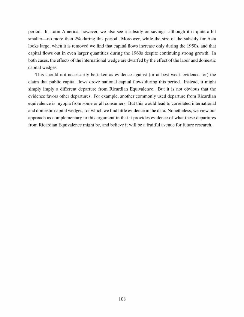
period. In Latin America, however, we also see a subsidy on savings, although it is quite a bitsmaller—no more than 2% during this period. Moreover, while the size of the subsidy for Asialooks large, when it is removed we find that capital flows increase only during the 1950s, and thatcapital flows out in even larger quantities during the 1960s despite continuing strong growth. Inboth cases, the effects of the international wedge are dwarfed by the effect of the labor and domesticcapital wedges.

This should not necessarily be taken as evidence against (or at best weak evidence for) theclaim that public capital flows drove national capital flows during this period. Instead, it mightsimply imply a different departure from Ricardian Equivalence. But it is not obvious that theevidence favors other departures. For example, another commonly used departure from Ricardianequivalence is myopia from some or all consumers. But this would lead to correlated internationaland domestic capital wedges, for which we find little evidence in the data. Nonetheless, we view ourapproach as complementary to this argument in that it provides evidence of what these departuresfrom Ricardian Equivalence might be, and believe it will be a fruitful avenue for future research.

108

Appendix F: Country Level Wedges

In this section, we present the labor and international wedges for each country in our Asia andLatin America samples and show that there are significant common components to these wedgesacross countries. We focus on these wedges because they can be measured without solving for theequilibrium of the model as they are defined by static first order conditions. We take the optimal-ity condition with resect to consumption from the pseudo-planners problem, and the labor-leisurecondition, and keep the parameters fixed at the value that was estimated originally for the cor-responding region. We then use individual country data to pin down these wedges for all LatinAmerican and Asian countries in our sample.

Figure 32 plots the Hodrick-Prescott trend of these international wedges. In this graph, note thata value of �0.05 is equivalent to a five percent tax on borrowing and a positive number representsa subsidy on borrowing. As can be seen in the plot, the wedges for individual countries sharea significant common component. Most important for our purposes, all countries except HongKong experience a significant decline in the tax on borrowing at the start of the sample, whichreverses around the beginning of the 1960s, and returns around the start of the 1970s. In the mid-1980s, all countries in the sample see an increase in the tax on international borrowing (a morenegative international wedge) which declines in the mid 1990s, before rising again around 1998 inthe aftermath of the Asian financial crisis.

These overall common patterns are quite close to those for the Asian region aggregate foundin Figure 3 of the paper. Note that, as a result of the fact that Japan and South Korea are thelargest countries in the region, the aggregate international wedge in the paper most closely followsthe individual international wedges for these two countries. This is particularly true in the earlyyears of the sample; in 1950, these two countries alone accounted for more than 95% of aggregateconsumption in the region.

109

Figure 32: International Wedge for Asian Countries

1960 1970 1980 1990 2000-0.1

-0.08

-0.06

-0.04

-0.02

0

0.02

0.04

Hong KongJapanSingaporeSouth KoreaTaiwan

Next, Figure 33 plots the Hodrick-Prescott trend (smoothed component) of the internationalwedge for the countries of our Latin America region. Once more, the plot reveals a significantcommon component in the international wedge for all of our countries. This pattern is especiallystriking in the latter half of our sample: all countries see an increase in the tax on borrowingbeginning somewhere around the middle of the 1980s as the Latin American debt crisis reached itspeak, and all see a recovery in the 1990s as these countries participated in Brady plans. The tax onborrowing rises again for all countries around the turn of the millennium.

110

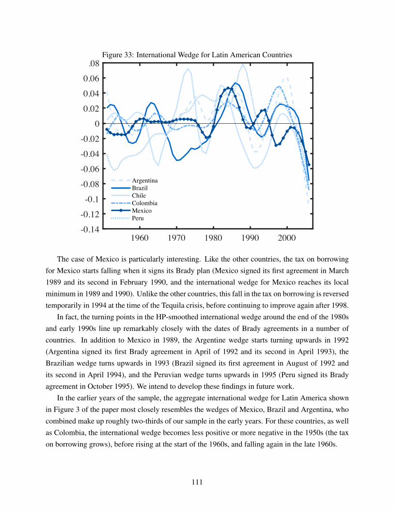
Figure 33: International Wedge for Latin American Countries

1960 1970 1980 1990 2000-0.14

-0.12

-0.1

-0.08

-0.06

-0.04

-0.02

0

0.02

0.04

0.06

.08

ArgentinaBrazilChileColombiaMexicoPeru

The case of Mexico is particularly interesting. Like the other countries, the tax on borrowingfor Mexico starts falling when it signs its Brady plan (Mexico signed its first agreement in March1989 and its second in February 1990, and the international wedge for Mexico reaches its localminimum in 1989 and 1990). Unlike the other countries, this fall in the tax on borrowing is reversedtemporarily in 1994 at the time of the Tequila crisis, before continuing to improve again after 1998.

In fact, the turning points in the HP-smoothed international wedge around the end of the 1980sand early 1990s line up remarkably closely with the dates of Brady agreements in a number ofcountries. In addition to Mexico in 1989, the Argentine wedge starts turning upwards in 1992(Argentina signed its first Brady agreement in April of 1992 and its second in April 1993), theBrazilian wedge turns upwards in 1993 (Brazil signed its first agreement in August of 1992 andits second in April 1994), and the Peruvian wedge turns upwards in 1995 (Peru signed its Bradyagreement in October 1995). We intend to develop these findings in future work.

In the earlier years of the sample, the aggregate international wedge for Latin America shownin Figure 3 of the paper most closely resembles the wedges of Mexico, Brazil and Argentina, whocombined make up roughly two-thirds of our sample in the early years. For these countries, as wellas Colombia, the international wedge becomes less positive or more negative in the 1950s (the taxon borrowing grows), before rising at the start of the 1960s, and falling again in the late 1960s.

111

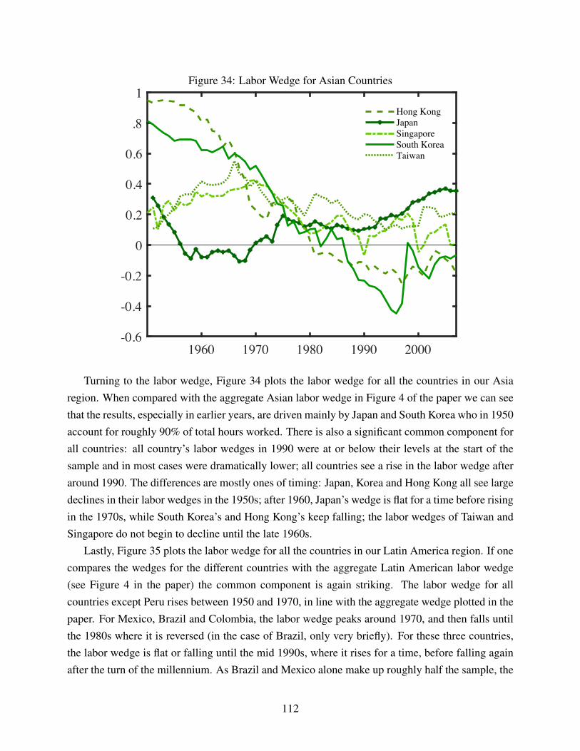
Figure 34: Labor Wedge for Asian Countries

1960 1970 1980 1990 2000-0.6

-0.4

-0.2

0

0.2

0.4

0.6

.8

1Hong KongJapanSingaporeSouth KoreaTaiwan

Turning to the labor wedge, Figure 34 plots the labor wedge for all the countries in our Asiaregion. When compared with the aggregate Asian labor wedge in Figure 4 of the paper we can seethat the results, especially in earlier years, are driven mainly by Japan and South Korea who in 1950account for roughly 90% of total hours worked. There is also a significant common component forall countries: all country’s labor wedges in 1990 were at or below their levels at the start of thesample and in most cases were dramatically lower; all countries see a rise in the labor wedge afteraround 1990. The differences are mostly ones of timing: Japan, Korea and Hong Kong all see largedeclines in their labor wedges in the 1950s; after 1960, Japan’s wedge is flat for a time before risingin the 1970s, while South Korea’s and Hong Kong’s keep falling; the labor wedges of Taiwan andSingapore do not begin to decline until the late 1960s.

Lastly, Figure 35 plots the labor wedge for all the countries in our Latin America region. If onecompares the wedges for the different countries with the aggregate Latin American labor wedge(see Figure 4 in the paper) the common component is again striking. The labor wedge for allcountries except Peru rises between 1950 and 1970, in line with the aggregate wedge plotted in thepaper. For Mexico, Brazil and Colombia, the labor wedge peaks around 1970, and then falls untilthe 1980s where it is reversed (in the case of Brazil, only very briefly). For these three countries,the labor wedge is flat or falling until the mid 1990s, where it rises for a time, before falling againafter the turn of the millennium. As Brazil and Mexico alone make up roughly half the sample, the

112

aggregate wedge in the paper follows this pattern.

Figure 35: Labor Wedge for Latin American Countries

1960 1970 1980 1990 20000

0.1

0.2

0.3

0.4

0.5

0.6

0.7

0.8

ArgentinaBrazilChileColombiaMexicoPeru

The other Latin American countries display similar patterns over this period, but with somewhatdifferent timing. Peru’s labor wedge is falling in the 1950s before rising slightly to 1980. After that,Peru’s labor wedge falls with Brazil’s in the 1980s, rises with the aggregate in the 1990s, and thenfalls after the turn of the millennium. Chile’s labor wedge also rises at the beginning of the samplebut does not reach a peak until roughly 1980, after which it falls with a pause in the mid 1990s thatcoincides with the increases in the labor wedge in the other countries. Argentina’s wedge falls inthe 1950s before rising until the late 1970s. After that, Argentina’s labor wedge is flat before risingwith other countries around 1990s, spiking at the turn of the millennium with its sovereign default,and then recovering sharply thereafter.

In sum, we find a significant common component in the international and labor wedges for eachgroup of countries. The differences that do exist tend to be confined to smaller countries, and aremostly matters of timing rather than differences in qualitative behavior. As a result, we take this isevidence in favor of our aggregation assumptions.

113

References Online Appendix

1. Backus, David and Mario Crucini. 2000. “Oil Prices and the Terms of Trade.” Journal ofInternational Economics, 50(1): 185-213.

2. Butlin, Matthew W. 1977. “A Preliminary Annual Database 1900/01 to 1973/74.” Researchdiscussion paper 7701, Reserve Bank of Australia.

3. Chinn, Menzie D. and Hiro Ito. 2006. “What Matters for Financial Development? CapitalControls, Institutions, and Interactions.” Journal of Development Economics, 81(1): 163-92,October.

4. Gollin, Douglas. 2002. “Getting Income Shares Right,” Journal of Political Economy, Uni-versity of Chicago Press, vol. 110(2), pages 458-474, April.

5. Gourinchas, Pierre-Olivier and Helene Rey. 2007. “International Financial Adjustment.”Journal of Political Economy, 115(4): 665-703, August.

6. Higgins, Matthew, Thomas Klitgaard and Cedric Tille. 2005. “The Income Implicationsof Rising U.S. International Liabilities.” Current Issues in Economics and Finance, FederalReserve Bank of New York, 11(Dec).

7. Hornstein, Andreas and Edward C. Prescott. 1993. “The Firm and the Plant in GeneralEquilibrium Theory.” in Robert Becker et al. eds., General Equilibrium, Growth, and TradeII: The legacy of Lionel McKenzie, San Diego: Academic Press.

8. Karabarbounis, Loukas and Brent Neiman. 2014. “The Global Decline of the Labor Share,”The Quarterly Journal of Economics, Oxford University Press, vol. 129(1), pages 61-103.

9. Lane, Philip R. and Gian Maria Milesi-Ferretti. 2001. “The External Wealth of Nations:Measures of Foreign Assets and Liabilities for Industrial and Developing Countries.” Journalof International Economics, 55(2): 263-94.

10. Lane, Phillip R. and Gian Maria Milesi-Ferretti. 2005. “Financial Globalization and Ex-change Rates.” IMF Working Paper No. 05/03.

11. Lane, Philip R. and Gian Maria Milesi-Ferretti. 2007. “The External Wealth of Nations MarkII: Revised and Extended Estimates of Foreign Assets and Liabilities, 1970-2004.” Journalof International Economics, 73(2): 223-50, November.

12. Magud, N. and S. Sosa. 2015. “Investment in Emerging Markets: We Are Not in KansasAnymore... Or Are We?” IMF Working Paper 15(77).

114

13. Marquez, Jaime and Lisa Workman. 2000. “Modelling the IMF’s Statistical Discrepancy inthe Global Current Account.” International Finance Discussion Papers No. 678, Board ofGovernors of the Federal Reserve System.

14. Sandleris, Guido and Mark L.J. Wright. 2013. “GDP-Indexed Bonds: A Tool to ReduceMacroeconomic Risk?” in Morten Balling, Ernest Gnan, and Johannes Holler eds., SUERFStudies, SUERF - The European Money and Finance Forum, No. 2013/5.

15. Sugimoto, Ichiro. 2011. The Economic Growth of Singapore in the Twentieth Century:Historical GDP Estimates and Empirical Investigations. World Scientific.

16. Tille, Cedric. 2003. “The Impact of Exchange Rate Movements on U.S. Foreign Debt.”Current Issues in Economics and Finance, 9(1).

115