bacterial degradation of dissolved organic carbon in … degradation of dissolved organic carbon ......
TRANSCRIPT
Bacterial degradation of dissolved
organic carbon in the water
column
An experimental and modelling
approach
The research presented is this thesis was carried out at the Department of
Theoretical Biology, Vrije Universiteit Amsterdam, The Netherlands and at
the Laboratory of Marine Microbiology, Geochemistry and Ecology,
University of Aix-Marseille II, Marseille France.
VRIJE UNIVERSITEIT
Bacterial degradation of dissolved organic carbon in the
water column
An experimental and modelling approach
ACADEMISCH PROEFSCHRIFT
ter verkrijging van de graad Doctor aan
de Vrije Universiteit Amsterdam,
op gezag van de rector magnificus
prof.dr. L.M. Bouter,
in het openbaar te verdedigen
ten overstaan van de promotiecommissie
van de faculteit der Aard- en Levenswetenschappen
op woensdag 23 januari 2008 om 13.45 uur
in de aula van de universiteit,
De Boelelaan 1105
door
Marie Eichinger
geboren te Mulhouse, Frankrijk

promotoren: prof.dr. S.A.L.M. Kooijman
prof.dr. J.C. Poggiale
Contents Chapter I: General introduction ..........................................................................1
I. The carbon cycle and the importance of processes of bacterial degradation
of dissolved organic matter in aquatic systems.................................................3
1. The role of dissolved organic carbon and of bacteria in the global
carbon cycle ...............................................................................................3
2. The dissolved organic carbon ....................................................................5
i. Composition .......................................................................................5
ii. Production ..........................................................................................8
iii. Spatial and temporal variability of DOC ............................................8
3. DOC utilisation by pelagic heterotrophic bacteria.....................................9
II. Modelling organic matter and bacterial dynamics ..........................................11
1. Utilisation of models with Michaelis-Menten kinetics ............................11
2. Utilisation of models with reserve ...........................................................13
3. Maintenance implementation...................................................................14
III. Objectives and thesis outline ..........................................................................16
Chapter II: Modelling DOC assimilation and bacterial growth efficiency
in biodegradation experiments: a case study in the Northeast
Atlantic Ocean ................................................................................19
I. Introduction.....................................................................................................21
II. Materials and methods ....................................................................................23
1. Experimental design ................................................................................23
i. Study area .........................................................................................23
ii. General design ..................................................................................23
iii. DOC and bacterial biomass estimations ...........................................25
2. Monod (1942) model ...............................................................................26
3. Comparison of methods for BGE estimation...........................................27
III. Results ............................................................................................................28
1. Model calibration and simulation ............................................................28
2. Sensitivity and robustness analyses .........................................................29
3. Parameters ...............................................................................................31
IV. Discussion.......................................................................................................37
1. Analysis of model results.........................................................................37
2. Biological analysis...................................................................................38
3. Experimental problems............................................................................38
4. Improvement of biogeochemical models.................................................39
V. Conclusion ......................................................................................................41
APPENDIX II-A....................................................................................................42
APPENDIX II-B ....................................................................................................43
Chapter III: Biodegradation experiments in variable environments:
substrate pulses and impact on growth efficiencies .................45
I. Introduction.....................................................................................................47
II. Material and methods......................................................................................50
1. General setup ...........................................................................................50
i. Precautions .......................................................................................50
ii. Experimental conditions ...................................................................50
2. Medium constitution, bacterial strain and preculture conditions .............51
3. Sampling method and variable measurements.........................................53
i. Sampling...........................................................................................53
ii. DOC .................................................................................................53
iii. POC ..................................................................................................54
iv. Optical density (OD) ........................................................................54
v. O2 consumption ................................................................................54
vi. Bacterial abundance..........................................................................55
4. DOC and POC data corrections ...............................................................56
i. Experiment B2..................................................................................57
ii. Experiment P ....................................................................................58
5. BGE estimation........................................................................................58
i. Experimental BGE estimation ..........................................................58
ii. BGE estimation from models ...........................................................59
III. Description of the experiments: initial conditions and reproducibility tests ...62
1. Determination of initial conditions and the pulse period.........................62
2. Reproducibility ........................................................................................63
i. Batch experiments ............................................................................63
ii. Pulse experiments.............................................................................63
IV. Identification of key processes........................................................................65
1. Autocorrelation of bacterial measurements .............................................65
2. Production of refractory material.............................................................68
3. Variation of the specific carbon content ..................................................71
4. Maintenance process................................................................................71
5. Instantaneous response to a perturbation .................................................71
V. Bacterial degradation of organic matter in a variable and a constant
environment: which system is the most efficient? ..........................................72
1. Experimental BGE estimation .................................................................72
2. BGE estimation from models ..................................................................72
i. Fitting ...............................................................................................72
ii. Comparison of BGE estimations from the three models ..................73
VI. Discussion.......................................................................................................77
VII. Conclusion ......................................................................................................82
APPENDIX III-A...................................................................................................83
APPENDIX III-B...................................................................................................87
APPENDIX III-C...................................................................................................92
Chapter IV: Application of the DEB theory on data obtained in
perturbed environment ..............................................................95
I. The DEB theory for micro-organisms ............................................................97
1. General concepts......................................................................................97
2. The DEB theory for bacteria....................................................................98
i. General considerations .....................................................................98
ii. Uptake ..............................................................................................99
iii. Reserve and structural body masses dynamics ...............................101
iv. Complete growth model .................................................................103
II. Mechanistic model simplification for implementation in biogeochemical
models: case of bacterial DOC degradation in a perturbed system...............104
1. Introduction ...........................................................................................104
2. Description of the experiments ..............................................................106
3. Specification of the DEB model ............................................................107
4. Simplification of the DEB model ..........................................................112
i. Variable aggregation ......................................................................112
ii. Comparison between the complete and the simplified models.......114
5. Bacterial growth in biogeochemical models..........................................115
6. Conclusion.............................................................................................116
III. Implementation of the respiration in DEB models .......................................117
1. Development of the O2 flux formulation ..............................................117
2. Implementation in the model .................................................................121
3. Calibration and simulation.....................................................................121
4. Conclusion.............................................................................................122
APPENDIX IV-A ................................................................................................124
APPENDIX IV-B.................................................................................................128
Chapter V: General conclusion and Perspectives ...........................................133
I. Bacterial growth efficiency...........................................................................134
II. Bacterial growth models ...............................................................................135
III. Experimentation – modelling coupling.........................................................136
IV. Perspectives ..................................................................................................137
References...........................................................................................................141
Summary - Samenvatting..................................................................................155
Acknowledgements ............................................................................................161
Acronym list .......................................................................................................163


1
CHAPTER I
General introduction
Chapter I 2
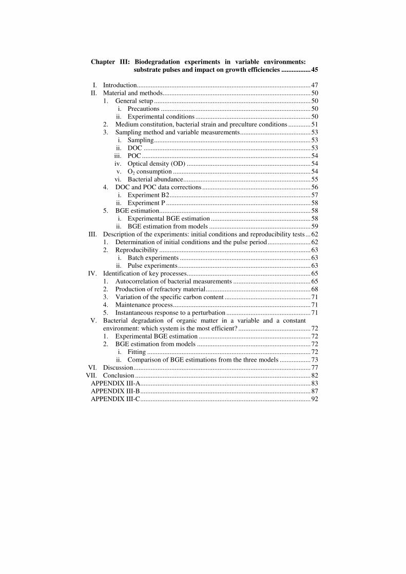
Figure I- 1: Reservoirs (Gt C) and flows (Gt C yr
-1) of the global carbon
cycle (Siegenthaler & Sarmiento 1993).
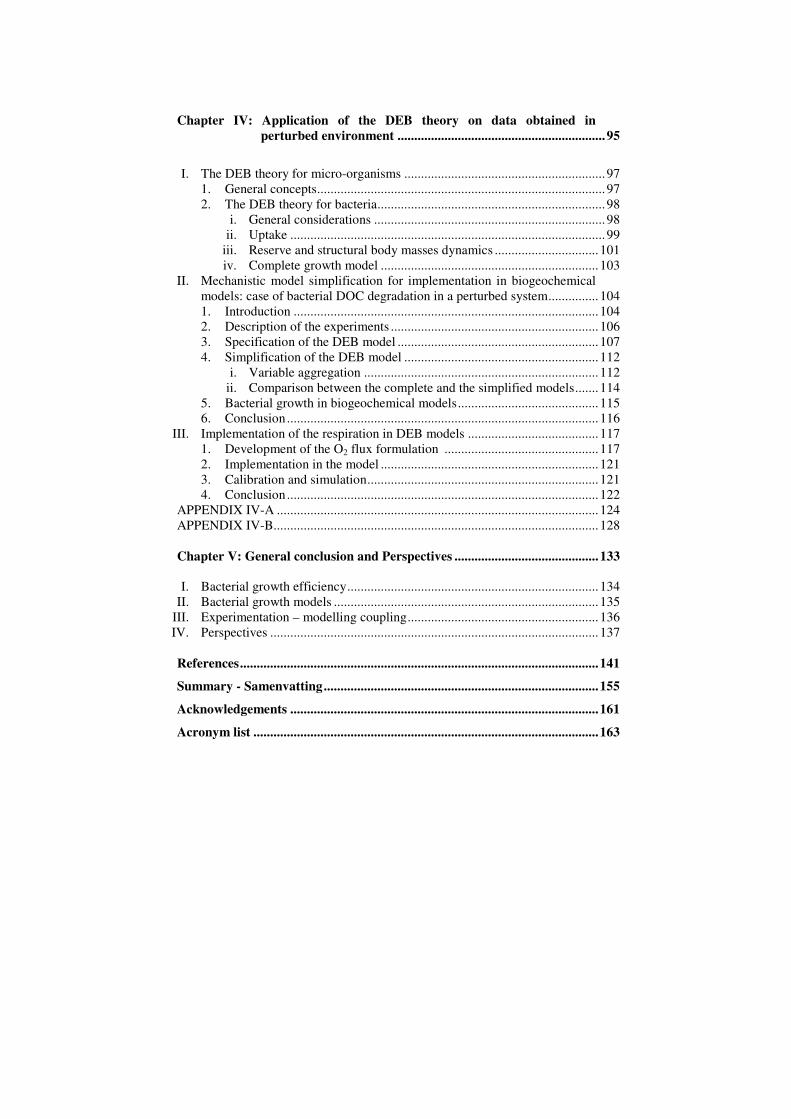
Figure I- 2: Size continuum spectrum of organic carbon, with the distinction
between the particulate phase (POC > 0.7 µm) and the dissolved one (DOC <
0.7 µm). Adapted from Verdugo et al. (2004).
General introduction
3
I. The carbon cycle and the importance of processes
of bacterial degradation of dissolved organic
matter in aquatic systems
1. The role of dissolved organic carbon and of bacteria in the
global carbon cycle
The global carbon cycle takes place inside and between the 4 spheres at
the surface of the planet: lithosphere, hydrosphere, biosphere and
atmosphere. The global stocks and flows of each of these reservoirs are given
in Figure I-1. The ocean, covering approximatively 70 % of the earth surface,
plays an important role in the carbon cycle and the global climate system.
Indeed, at the global scale, seawater is an important component of the carbon
cycle and constitutes one of the larger carbon reservoirs: the dissolved
inorganic carbon amounts to 40 000 Gt C, thus approximatively 6 times the
amount of atmospheric carbon dioxide (CO2).
Carbon is fractionated into 2 categories: inorganic carbon (IC) and
organic carbon (OC). IC is associated to compounds which are or were not
living and which do not contain any C-C or C-H link, as for example the
carbon from CO2 or those from carbonate calcium CaCO3. OC is produced by
living organisms and is chemically linked to other carbon atoms or to
elements as hydrogen (H), nitrogen (N) or phosphor (P). OC is subdivided
into 2 classes: dissolved organic carbon (DOC) and particulate organic
carbon (POC). Separation between both stocks is based on their size: all
compounds that pass a filter with a given retention size (generally 0.7 µm)
are considered as dissolved, the rest as particulate (Figure I-2). However,
some living organisms, thus particulate, such as bacteria, are in the boundary
of this separation and may partially be considered as DOC.
From a biological point of view, the carbon cycle typically starts from the
conversion of CO2 and other inorganic nutrients to OC and O2 by
photosynthesis (Figure I-3). In pelagic environments, photosynthesis is
realised by phytoplankton, marine plants and algae but also by other
autotrophic organisms such as cyanobacteria. This first step requires light and constitutes the primary production. OC produced by primary production can
be consumed by higher trophic levels such as zooplanktonic organisms and
fishes. DOC and POC are produced all along this trophic chain. DOC
includes excretion of small molecules and POC includes fecal pellets. POC
can be transformed into DOC according to several processes such as
dissolution and enzymatic processes. DOC is used by heterotrophic bacteria
Chapter I 4
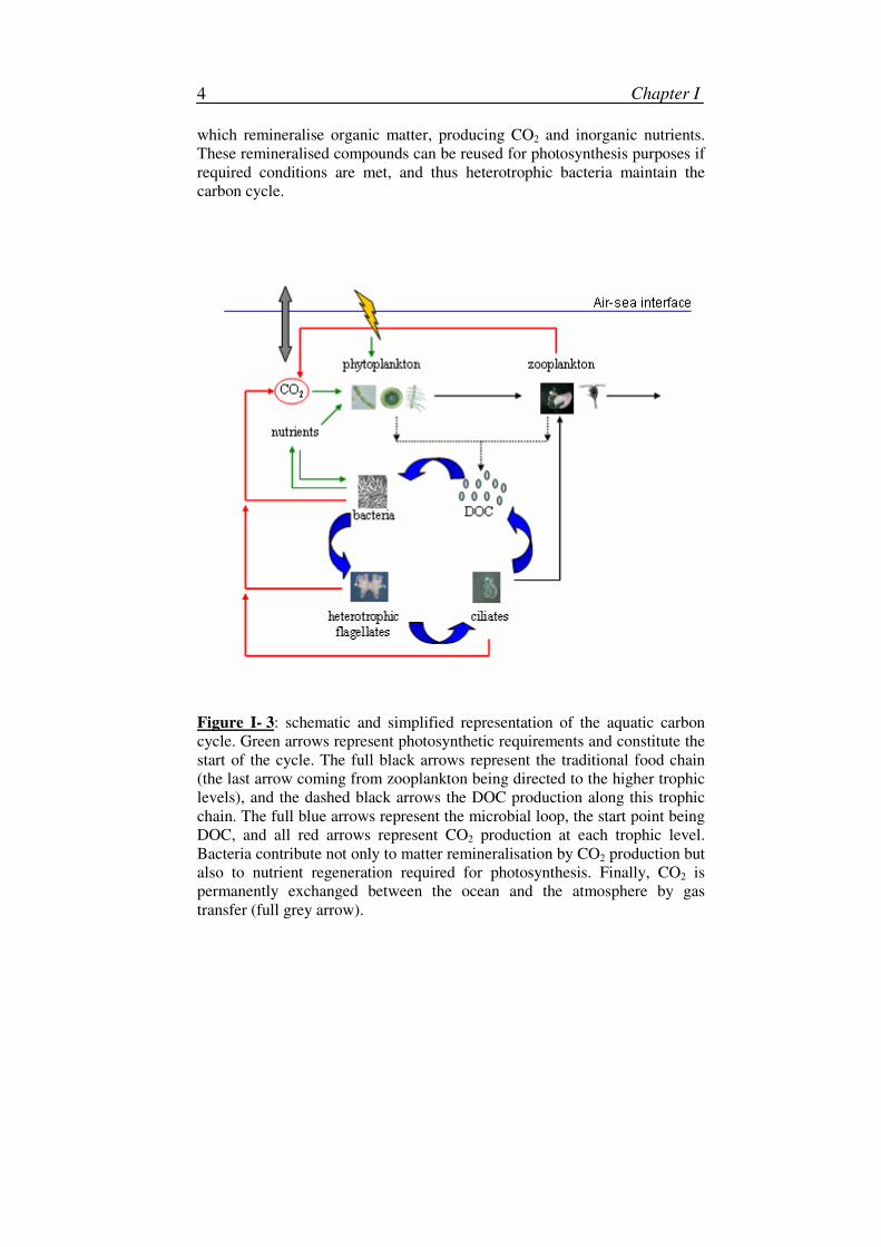
which remineralise organic matter, producing CO2 and inorganic nutrients.
These remineralised compounds can be reused for photosynthesis purposes if
required conditions are met, and thus heterotrophic bacteria maintain the
carbon cycle.
Figure I- 3: schematic and simplified representation of the aquatic carbon
cycle. Green arrows represent photosynthetic requirements and constitute the
start of the cycle. The full black arrows represent the traditional food chain
(the last arrow coming from zooplankton being directed to the higher trophic
levels), and the dashed black arrows the DOC production along this trophic
chain. The full blue arrows represent the microbial loop, the start point being
DOC, and all red arrows represent CO2 production at each trophic level.
Bacteria contribute not only to matter remineralisation by CO2 production but
also to nutrient regeneration required for photosynthesis. Finally, CO2 is
permanently exchanged between the ocean and the atmosphere by gas
transfer (full grey arrow).
General introduction
5
It is widely recognised that heterotrophic bacteria play a predominantly
role in the carbon cycle. Indeed, they represent the most important living
biomass in aquatic ecosystems. They also constitute the major DOC
consumers (Pomeroy 1974), this latter being the second most important stock
of bioreactive carbon in ocean (680 – 700 Pg C) (Williams & Druffel 1987,
Hansell & Carlson 1998) after the very large stock of dissolved IC (38 000
Pg C) (Hansell 2002). DOC dynamic is thus important for understanding
global carbon cycle and changes of atmospheric CO2, the most critical
greenhouse gas on our planet (Siegenthaler & Sarmiento 1993). DOC, after
being consumed by heterotrophic bacteria, is either incorporated in the food
chain or respired as CO2. Bacteria represent thus either a sink or a source of
carbon. DOC may also be photooxidised and remineralised in the surface
layer (Tedetti 2007 et al. and references therein) or exported into the deep
ocean by winter convection of the surface water masses (Copinmontegut &
Avril 1993).
2. The dissolved organic carbon
i. Composition
DOC has a very heterogeneous nature and has thus been classified into
different categories, which differ according to the studies. Some authors
classify DOC pools between material that disappears rapidly to that which
accumulates (Anderson & Williams 1999, Christian & Anderson 2002).
Three distinct pools have been determined according to their reactivity
towards heterotrophic bacteria: labile DOC (L-DOC) that is consumed in
hours to days, semi-labile DOC (SL-DOC) that has a turnover time of weeks
to years and refractory DOC (R-DOC) that has a turnover rate of millennia
(Williams & Druffel 1987, Bauer et al. 1992, Druffel et al. 1992, Carlson &
Ducklow 1995, Hansell et al. 1995, Carlson & Ducklow 1996, Carlson
2002). L-DOC represents DOC fraction which may be directly utilised by
bacteria whereas SL-DOC needs bacterial enzymatic activity to be
transformed in L-DOC and being consumed. R-DOC can be transformed into
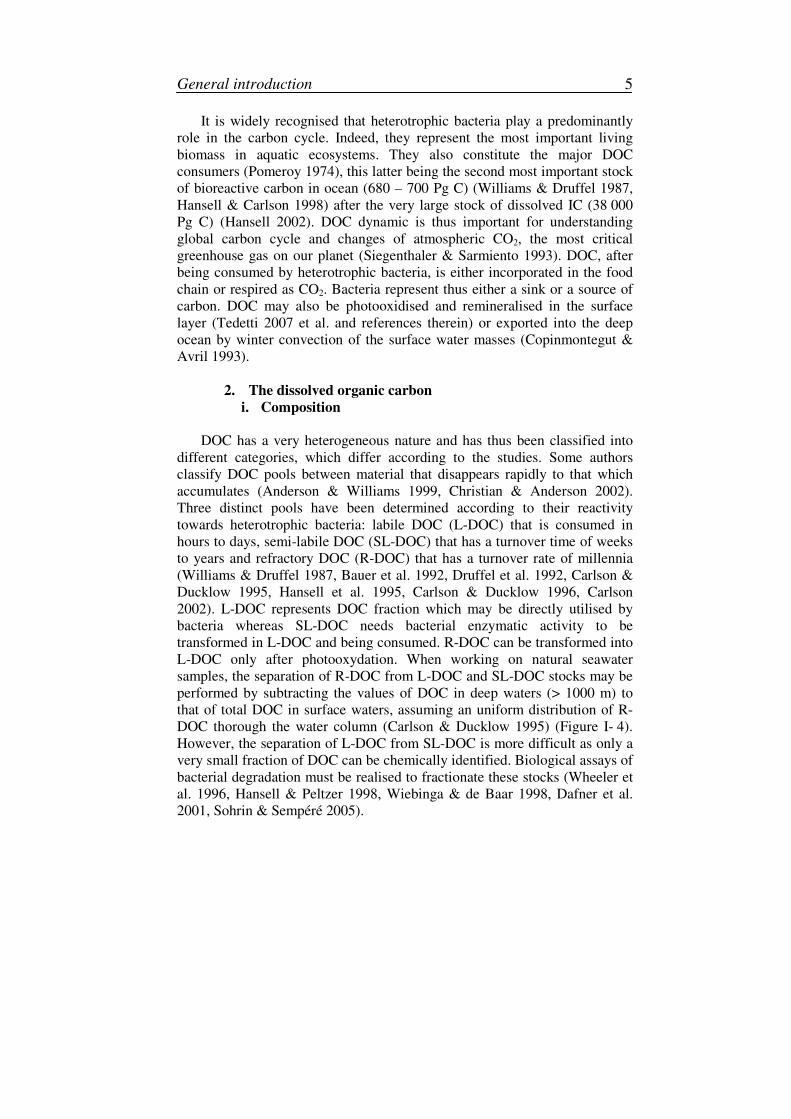
L-DOC only after photooxydation. When working on natural seawater
samples, the separation of R-DOC from L-DOC and SL-DOC stocks may be
performed by subtracting the values of DOC in deep waters (> 1000 m) to
that of total DOC in surface waters, assuming an uniform distribution of R-
DOC thorough the water column (Carlson & Ducklow 1995) (Figure I- 4).
However, the separation of L-DOC from SL-DOC is more difficult as only a
very small fraction of DOC can be chemically identified. Biological assays of
bacterial degradation must be realised to fractionate these stocks (Wheeler et
al. 1996, Hansell & Peltzer 1998, Wiebinga & de Baar 1998, Dafner et al.
2001, Sohrin & Sempéré 2005).
Chapter I 6
DOC (µM)
Refractory
Labile
Semi-labile
De
pth
(m
)
0
200
400
600
800
1000
0 20 40 60 80
DOC (µM)
Refractory
Labile
Semi-labile
De
pth
(m
)
0
200
400
600
800
1000
De
pth
(m
)
0
200
400
600
800
1000
0 20 40 60 800 20 40 60 80
Figure I- 4: The distribution of DOC in the water column (Anderson &
Williams 1999). L-DOC is only present in small concentrations in the surface
layer.
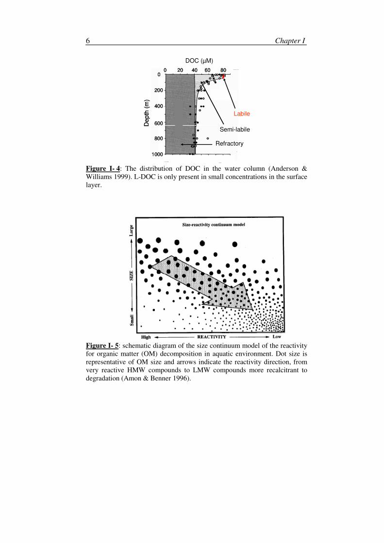
Figure I- 5: schematic diagram of the size continuum model of the reactivity
for organic matter (OM) decomposition in aquatic environment. Dot size is
representative of OM size and arrows indicate the reactivity direction, from
very reactive HMW compounds to LMW compounds more recalcitrant to
degradation (Amon & Benner 1996).
General introduction
7
DOC may also be fractionated with respect to their molecular weight
(Amon & Benner 1996). Low molecular weight (LMW) compounds, with a
size less than 1 kDa, can be distinguished from DOC compounds with a high
molecular weight (HMW), with a size between 1 kDa and 30 kDa, and from
DOC with a very high molecular weight (VHMW) with a size greater than 30
kDa. However, the relationship between this latter classification and the
previous one based on lability is not very clear. Most studies assimilate
LMW compounds to labile material, and inversely HMW compounds to
more refractory material (Saunders 1976). In contrast, some studies
demonstrate that HMW compounds are more reactive (Amon & Benner
1996) and a new size continuum model has been created, where the
bioreactivity of DOC decreases with decreasing size (Figure I- 5). Authors
supposed that freshly produced organic matter (OM) is HMW and that during
decomposition OM continuously becomes less bioreactive and smaller in
physical size, giving rise to LMW molecules with a low reactivity (Amon &
Benner 1996).
DOC may also be classified with respect to its chemical nature
(carbohydrate, lipid, nucleic acid), but currently only approximatively 30 %
of the bulk DOC pool have been chemically characterised. In order to try to
understand which compounds are preferentially utilised by bacteria, and thus
to determinate the labile nature of these compounds, numerous authors have
used biodegradation experiments with seawater samples by adding model
compounds. Inorganic nutrients are also often added in these cultures. The
observation that added inorganic nutrients do not stimulate bacterial
production or DOC utilisation indicates that growth is limited by the OC
availability (Carlson & Ducklow 1996, Carlson et al. 2002). Other
experiments showed that compounds such as glucose, dissolved free amino
acids (DFAA) and natural plankton extracts stimulate bacterial production as well as OM utilisation with turnover rates of some days (Cherrier et al.
1996). These compounds may thus be classified as L-DOC. Carlson (2002)
states that the most biologically reactive organic compounds in seawater
include dissolved free compounds such as neutral monosaccharides (MCHO)
and DFAA. Another experiments, where OM addition consists of plankton
extracts, showed that only 28 % of this extract have been chemically
characterised and consists of DFAA, dissolved combined amino acids
(DCAA) and MCHO (Cherrier & Bauer 2004). In addition, only 31 % of this
added DOC were used by bacteria during short biodegradation experiments,
and may thus be classified in L-DOC, but only 75 % of the utilised
compounds have been chemically characterised (Cherrier & Bauer 2004).
This study proves thus the complexity of associating chemical compounds
with a labile nature of OC.
Chapter I 8
ii. Production
Numerous mechanisms of DOC production have been highlighted. The
main source of DOC production seems to come from release by
phytoplankton (Nagata 2000). However, other processes are involved in
DOC production, as egestion, excretion and “sloppy feeding” by grazers, and
cell lysis induced by viruses (Nagata 2000, Carlson 2002). The quantitative
role of DOC release by phytoplankton is assessed by the percent extracellular
release (PER). This latter have been extensively studied and present a high
variability depending on whether it was estimated from phytoplanktonic
cultures or from natural seawater. PER fluctuates between 2 and 10 % in
cultures (Nagata 2000) and between 0 and 80 % in the field for a variety of
coastal and oceanic systems (Carlson 2002). Grazers also participate
substantially to DOC production. Indeed, the magnitude of potential DOC
release by protozoa, that feed on small phytoplankton and bacteria, is
equivalent to or even exceeds that of phytoplankton (Nagata 2000). In
addition, zooplankton, i.e. grazers that feed on large phytoplankton, could
release DOC by four main processes: excretory release, egestion, sloppy
feeding (breakage of large prey during handling and feeding) and release
from fecal pellets (Carlson 2002). Production rates are highly variable
according to the considered process (Nagata 2000). Viral lysis plays also an
important role among these DOC production processes. Finally, even bacteria
may participate to DOC production. Indeed, structural components of
bacterial cells including membranes and peptidoglycan can be introduced to
seawater as DOC during bacterial death due to protozoan grazing and viral
infection (Nagata & Kirchman 1999).
However, we don’t get any information about DOC lability else than via
the process by which it is produced. The labile character of a compound is
very difficult to estimate. Indeed, if DOC consumption is studied in cultures
including one DOC producer and bacteria, these flows being direct, we
cannot measure the fraction of DOC that is really assimilated by bacteria. On
the other hand, studying only DOC production does not allow estimating its
potential utilisation by bacteria.
iii. Spatial and temporal variability of DOC
From a general point of view, DOC concentration is higher in the surface
layer than in deep waters. In deep waters, DOC concentration is considered
constant around 34 µM C but may vary slightly due to marine currents. For
example, 29 % decrease in DOC concentration has been observed between
north of the North Atlantic and north of the North Pacific (Hansell & Carlson
General introduction
9
1998). Surface concentrations are more variable, due to more pronounced
spatial and temporal influences. The DOC mean surface concentration may
be estimated to 90 µM C (Hansell 2002). Its spatial variation may be affected
by physical phenomenona such as (1) upwelling which will reduce the DOC
concentration, (2) terrigenous inputs such as the highly concentrated DOC
inputs by riverines. In this latter case, the DOC concentration may exceed
200 µM C. The temporal DOC variation is principally due to seasonal
phytoplankton blooms. However, the magnitude of this variability differs
with the region. So, strong increases in DOC concentration are characteristic
of high latitude systems which receive high fresh nutrients inputs during
winter periods. For example, the DOC concentration in surface waters
increases from 42 µM C in winter to 65-70 µM C in summer in the Ross Sea
(Carlson et al. 1998). In oligotrophic zones, with medium latitudes, oceans do
not exhibit the same seasonality (Hansell 2002). The changes in DOC
concentration is on average only about 3-6 µM C, that is small amplitudes
compared to the high latitude systems (Hansell 2002). This phenomenon is
due to mixing between surface and deep waters, with a small DOC
concentration, when primary production is high. Consequently, when
stratification becomes established with the heating of the top layer, the
phytoplanktonic bloom will cease and the DOC concentration increases again
to normal levels. Oceanic systems at low latitude do not undergo winter
refreshment of the surface layer and thus seasonality in DOC concentration
(Hansell 2002). It is therefore important to be aware that spatial and temporal
variabilities are tightly coupled, implying that impacts from spatial or
temporal variability are difficult to discriminate.
3. DOC utilisation by pelagic heterotrophic bacteria
Heterotrophic bacteria are considered as major consumers and
remineralisers of dissolved organic matter (DOM) in the ocean (Pomeroy
1974). They also represent a very dynamic compartment in the interaction
between geosphere, hydrosphere and biosphere and as such has the potential
to influence the global carbon cycle and climate change (Farrington 1992).
The interactions between DOM and bacteria play a central role in the aquatic
carbon cycle; thus, the factors regulating DOM production and consumption
profoundly influence carbon fluxes (Amon & Benner 1996). Moreover, since
Azam et al. (1983) have highlighted the ecological role of bacteria in the
water column, numerous studies have tried to understand how bacteria
utilised and transformed DOM.
Chapter I 10
The bacterial growth efficiency (BGE) is a factor allowing the
determination of the DOM utilised by bacteria for their growth, the remaining
being remineralised. Indeed, at low BGE, more DOM will be remineralised,
keeping the nutrient cycling within the microbial cycle; at high BGE the OM
is transferred from the dissolved phase to the particulate phase and with
increased probability into the larger trophic size fractions (del Giorgio &
Cole 1998, del Giorgio & Duarte 2002, Cajal-Medrano & Maske 2005). BGE
allows thus estimating bacterial impact in marine ecosystems as carbon
source or sink. Numerous environmental factors may affect BGE (del
Giorgio & Cole 1998): DOC quality in term of molecular weight (Amon &
Benner 1996), chemical nature of DOC (Carlson & Ducklow 1996, Cherrier
et al. 1996, Cherrier & Bauer 2004), substrate C:N ratio (Goldman et al.
1987), distance of the study site from the shore (del Giorgio & Cole 1998, La
Ferla et al. 2005), season (Reinthaler & Herndl 2005, Eichinger et al. 2006),
temperature (Rivkin & Legendre 2001) and depth (Eichinger et al. 2006).
However, BGE comparison between studies is made difficult due to the
diversity of methods used and the utilisation of conversion factor.
BGE is estimated from experimental data generally obtained from batch
cultures. BGE is calculated from bacterial production (BP), bacterial
respiration (BR) and/or bacterial carbon demand (BCD) according to the
following formula BGE=BP/BCD where BCD=BP+BR (Carlson & Ducklow
1996, del Giorgio & Cole 1998, Rivkin & Legendre 2001, Sempéré et al.
2003, Cherrier & Bauer 2004). BP may be estimated from tritiated leucine or
thymidine incorporation, but its estimation requires the utilisation of
conversion factors which are not necessarily constant. BR is estimated from a
linear regression on the increasing CO2 concentration in incubations that last
few days, or more generally from a linear regression on the decreasing O2
concentration. However, the conversion from O2 consumption to CO2
production which corresponds to BR requires the utilisation of an assumed
respiratory quotient (RQ). This latter is considered constant and is often
approximated to 1 for sake of simplicity or to 0.8 as a mean of literature
values (Sempéré et al. 2003). BCD is calculated either as the sum of BP and
BR or as the decrease of DOC in cultures. However, BGE values resulting
from the estimation of BCD as BP+BR or as the rate of decrease of DOC
concentration may be different (Cherrier et al. 1996). Consequently, the sole
utilisation of a conversion factor biases BGE estimation.
General introduction
11
II. Modelling organic matter and bacterial dynamics
This section focuses on the different models which have been used to
describe bacterial growth utilising DOC as nutritive resource. Since Azam et
al. (1983) allocated the term microbial loop for the set of interacting
processes responsible for the recycling of dead OM into particulate biomass,
there was an increasing number of studies trying to estimate the carbon flow
through microbial loop. Heterotrophic bacteria represent the major organisms
that consumed and remineralised DOM (Pomeroy 1974) and are the central
component of the microbial food web (Legendre & Rassoulzadegan 1995).
Consequently, an understanding of the relevant aspects of bacterial
physiology is a prerequisite for any detailed understanding of how
heterotrophic bacteria interact with DOC and organisms at other trophic
levels in the microbial loop (Martinussen & Thingstad 1987). Many
experimental studies were conducted and models proposed to explore the
bacterial link-sink problem (Touratier et al. 1999). Mathematical models
provide tools which allow investigation of complex dynamics such as
microbial food webs. However, the design of a particular model may vary
greatly and depends on the particular purpose of the modelling exercise, as
modelling of an ecosystem as a whole and modelling of the physiology of the
individual physiology are carried out with different objectives and often
using different approaches (Davidson 1996). We have thus decided to
describe the various models in relation to their complexity at the level of
bacterial physiology, and not in relation to the complexity of the global
model, that is to say if the considered study presents a simple bacterial
growth model or an ecosystem model dealing with numerous parameters and
state variables. The bacterial growth formulation may however be the same
depending on whether the model is a growth model or a trophic chain model.
Models describing carbon utilisation by bacteria were developed by various
authors and the system complexity varies (Cajal-Medrano & Maske 1999)
from simple models with 2 state variables (Monod 1942) to very complex
bioenergetic models with many state variables (Vallino et al. 1996).
1. Utilisation of models with Michaelis-Menten kinetics
The Monod (Monod 1942) model uses Michaelis-Menten (Michaelis &
Menten 1913) kinetics and is certainly the most extensively used formulation
for describing bacterial growth with DOC as nutritive resource. This model
assumes that substrate (X) is directly and instantaneously assimilated by
bacteria (B) with a constant growth efficiency (BGE). The substrate
Chapter I 12
utilisation is described by a Michaelis-Menten formulation with a maximum
specific assimilation rate (Vmax) and a half-saturation constant (K):
max
max
dX XV B
dt K X
dB XBGE V B
dt K X
= −
+
=
+
This model assumes that a proportion BGE of the assimilated substrate is
utilised for growth, and that the complementary proportion (1-BGE) is thus
used for respiration. At the bacterial level, this model has been used to
describe in situ data on growth and L-DOC utilisation (Eichinger et al. 2006),
as well as in a chemostat-type theoretical study dealing with 2 potentially
limiting substrates (C and N) (Thingstad & Pengerud 1985). The Monod
model has been more extensively used in studies at a wider scale, i.e. studies
describing the microbial loop or global models aiming to represent elemental
cycles in marine systems. Among these studies, microbial loop models
including heterotrophic bacteria have been realised, the aim being generally
to investigate the carbon flow through microbial loop and the interactions
between bacteria and other organisms constituting the microbial loop.
However, most of these works investigated models at their steady-state and
compare model outputs with stock data (Taylor & Joint 1990, Blackburn et
al. 1996, Anderson & Ducklow 2001) or considered the model only on a
theoretical point of view without comparison with data (Thingstad &
Pengerud 1985). In addition, parameter values of the four last cited models
came from literature or were assumed. This latter fact, in addition to the
absence of model validation with dynamical data, complicates the evaluation
of the pertinence of these models in the context of this thesis. Moreover,
substrate quality was taken into account but the various studies did this in
different ways: quality may be converted to a lability, which is expressed as a
fraction of the DOC production by the considered source (phytoplankton
exudation, bacterial lysis, grazing) (Taylor & Joint 1990, Anderson &
Ducklow 2001) or taken to be a function of elemental C:N ratios (Thingstad
& Pengerud 1985, Blackburn et al. 1996).
Finally, many studies, focusing mainly on cycling of elements in marine
systems, have used this formulation to describe DOC utilisation by bacteria
(Davidson 1996, Christian & Anderson 2002). Some studies specifically
investigated oceanic DOC cycling and have used a Monod-type formulation
(Connolly & Coffin 1995, Anderson & Williams 1998, 1999), a simplified
Monod-type formulation (Bendtsen et al. 2002), or a slightly more
complicated Monod-type formulation by adding for example a temperature-
General introduction
13
dependant relationship (Bissett et al. 1999) or by taking into account a
carbon absorption threshold (Tian et al. 2000). All these models, except the
last one, considered several DOC labilities. However, even if the global
dynamics of these models match DOC distribution in marine systems well,
the validity of these models is limited due to (1) the parameter values that
were assumed or taken from literature and (2) the comparison of model
outputs with data comprising either only few variables of the model or few
data points. Other ecosystem models utilised also Monod-type formulations
for the DOC utilisation by bacteria, but without specific attention for the
carbon cycle (Billen & Becquevort 1991, Vallino 2000, Spitz et al. 2001,
Lancelot et al. 2002, Raick et al. 2005).
2. Utilisation of models with reserve
The ability of carbon storage by heterotrophic bacteria has been demonstrated
for carbon limited systems (Baxter & Sieburth 1984) as well as for systems
not limited by carbon availability (Kooijman 2000). Production and
accumulation of carbon products, such as polymeric carbohydrates, has been
shown to be a survival mechanism to dispose of the excess MCHO taken up
(Baxter & Sieburth 1984). This storage capacity provides an explanation of
the continued cell growth after depletion of the substrate (Martinussen &
Thingstad 1987). This experimental result has thus to be taken into account in
models simulating bacterial growth and utilisation of carbon substrate. To
take this storage material into consideration, growth models often used the
Droop (Droop 1968) model or an adaptation of this latter. This model has
been originally constructed to describe nutrient-limited growth of a
monospecific phytoplankton strains. Since then, it has been extensively used
and extended to study heterotrophic bacteria. Some studies have used an
adapted form of this model to describe carbon utilisation and bacterial growth
in chemostat-type theoretical situations (Thingstad & Pengerud 1985,
Thingstad 1987) or in comparison with batch or chemostat data (Martinussen
& Thingstad 1987). In these studies, this model has been used to describe
limitation by nitrogen (N), phosphor (P) or carbon (C). This allows flexibility
in biomass composition in term of C, N and P, whereas Monod model
assumes constant composition. In this kind of model, growth depends on a
surplus pool of nutrients inside the cell, named cell quota, and not on the
outside concentration of limiting nutrient directly as in Monod model. The
growth rate is controlled only by the cell quota (C, N or P) which is closest to
its minimum value. In the works cited previously, model formulation for the
substrate utilisation and growth of bacterial biomass has evolved in the
course of years and has been adapted to match experimental results. The
model considered different formulations for the growth in term of biomass
Chapter I 14
(C, N or P) and the growth in term of cell number which only depends of one
of the three elements.
Contrary to the Monod model, quota models have been rarely used in
microbial loop or ecosystem models. Some microbial loop models have used
cell quota (Baretta-Bekker et al. 1998) to describe element fluxes and to
allow bacteria using inorganic nutrients, a capability not utilised in their
previous model; Baretta-Bekker et al. (1994) allowed only OC utilisation. A
complex biogeochemical model, following from the ERSEM model of
Baretta-Bekker et al. (1998), used also the notion of cell quota. This was to
decouple OC assimilation from nitrogenous and phosphorous nutrient
utilisation rather than to create material storage in the cell. Contrary to the
studies of Thingstad et al. cited previously where each quota comprises only
1 element (C, N or P) and where growth depends on the ratio between the
minimum quota and the current quota value, cell quota correspond here to
C:N and C:P ratios and permit to determine the limiting element.
Dynamic energy budget (DEB) theory (Kooijman 2000) considers
storage of nutrients as well as energy substrates. This theory provides laws
for energy and substrate absorption and their utilisation by organisms. One
organism is quantified by at least 2 state variables: reserve and structure (see
chapter IV). Reserve is thus considered as a state variable as well and the
number of reserves might equal that of nutrients. This theory has been
extensively applied to the growth of heterotrophic bacteria (Kooijman et al.
1991, Hanegraaf & Muller 2001, Brandt et al. 2003, Brandt et al. 2004) and
to the growth of bacteria implied in prey-predator interactions and in small
trophic chains (Kooi & Kooijman 1994, Kooijman et al. 1999, Hanegraaf &
Kooi 2002). In all of these studies models have been compared to data and
match very well. However, DEB theory has currently not been used for
describing microbial loop or complex ecosystems, certainly because resulting
models are complex and the calibration of their numerous parameters and
state variables is complicated.
3. Maintenance implementation
Some of the models cited previously used also the notion of maintenance
to translate the fact that organisms provide energy not only for biosynthetic
processes producing growth but also for physiological activity that does not
produce new biomass but maintain cell integrity (Cajal-Medrano & Maske
2005). This energy is utilised for the turnover of cell constituents, ionic
equilibrium and repair processes (Cajal-Medrano & Maske 1999). This
maintenance activity is decoupled from growth and is necessary for cell
General introduction
15
survival even if concentration of bioavailable substrate is not sufficient to
ensure growth. First authors having pointing out maintenance requirements
were Herbert (1958), Marr et al. (1963) and Pirt (1965). This maintenance
activity is often represented in models by respiration, accounting for a term
of basal respiration and one of activity linked to the growth. Cajal-Medrano
and Maske (1999, 2005) have used a model which links the respiration rate,
taking into account both terms, and the growth rate together. These studies
aimed to interpret published data concerning BGE values obtained with
natural bacterial population from temperate, pelagic systems. However, these
studies did not compare the model with dynamical data of DOC and bacteria.
Other studies, based on bacterial growth, have taken the maintenance process
into account in models. Some of these models assessed the influence of
substrate quality, in terms of C:N ratio, on growth, respiration and excretion,
but they described growth according to Michaelis-Menten kinetics (Touratier
et al. 1999). Other studies have also incorporated maintenance as respiration;
contrary to most studies, this latter is realised from carbon cell quota and not
directly from assimilated substrate (Martinussen & Thingstad 1987,
Thingstad 1987). This model has been calibrated and compared to steady-
state and transient data, coming from batch and chemostat experiments, and
showed a good match.
Some microbial loop models also take maintenance into account by
fractioning respiration into a part dedicated to growth and the other one
linked to maintenance (Baretta-Bekker et al. 1994, Blackburn et al. 1996,
Baretta-Bekker et al. 1998). The presence of maintenance in bacteria is rare
in ecosystem models. Connolly and Coffin (1995) took basal respiration into
account, but not that linked to growth. In most other models, growth is
realised with a constant fraction BGE, thus considering or assuming that
respiration is the part of the assimilated carbon not utilised for growth, which
means that respiration is only linked to growth by a fraction (1-BGE)
(Anderson & Williams 1998, 1999, Bissett et al. 1999, Tian et al. 2000,
Vallino 2000, Spitz et al. 2001, Pahlow & Vézina 2003, Raick et al. 2005).
DEB theory is based on 3 main processes: assimilation, maintenance and
growth (Kooijman 2000). Consequently, all models constructed from this
theory account for cell maintenance. Maintenance costs are also paid from
reserve. Contrary to all models cited previously that include maintenance,
DEB theory, being based on energy, does not identify maintenance to
respiration and maintenance costs can be paid in different ways.
Consequently, maintenance may result in biomass loss and/or in product
formation that are not necessary CO2 (see chapter IV).
Chapter I 16
III. Objectives and thesis outline
This thesis aims to investigate growth of pelagic heterotrophic bacteria
that utilise DOC as nutritive resource by using both experimental and
modelling approaches. Two main axes merge from this work: (1) the study of
growth models, constructed from experimental results, with a view to
implement them in ecosystem models, and (2) the investigation of the
environmental factors influencing the BGE with these models. The main
objective consists of the study of bacterial growth in different environmental
contexts and to deduce a suitable mathematical formulation for describing the
interaction between growth and DOC to include this in a biogeochemical
model later on. To do that, a strong coupling between experimentation and
modelling was required. The various growth models described previously,
with different levels of complexity, have been studied and have been
confronted to data, these latter coming either from natural seawater or from
experiments in artificial conditions.
This thesis is divided into 4 parts.
The first chapter concerns the utilisation of the Monod model for
describing bacterial growth and DOC assimilation in in situ conditions. 36
biodegradation experiments have been performed during the POMME
program in Atlantic Ocean, corresponding to several water depths and
seasons. The various measurements realised during the experiments allowed
the determination of bacterial biomass and DOC concentration dynamics for
each experiment. However, the small number of measurements did not allow
the use of a mechanistic model. We have thus decided to utilise the Monod
model as it takes only 2 state variables and 3 parameters into account.
Moreover, this model is the most used to describe the utilisation of carbon
substrate by heterotrophic bacteria in biogeochemical models, and we were
thus able to test its pertinence towards in situ data. This model has been
calibrated for each experiment and we were thus able to estimate BGE and
the assimilation rate for each of them. The model parameters, including BGE,
varied according to depth and season and demonstrated that the Monod
model is not sufficient for describing the DOC utilisation by bacteria in
biogeochemical models.
The second chapter concerns the investigation of biodegradation in a
perturbed system, carried out with an artificial medium and a monospecific
bacterial strain using a single carbon substrate. Previous experiments required
a lot of assumptions to apply a model, which complicates further analysis and
General introduction
17
interpretation of results. In addition, the experimental setup did not allow the
application of a complex model. Utilisation of artificial culture medium
permitted the control of experimental conditions and thus allowed not only
numerous measurements and application of less restrictive models, but also
applying experimental perturbations in order to be close to natural conditions
from a qualitative point of view. This chapter focuses especially on the
comparison of 2 experiments carried out under the same experimental
conditions, the difference being the input regime of the carbon substrate in
the batch cultures. In the first experiment, whole substrate was loaded as soon
as the experiment began, as for the experiments realised during the POMME
program. In the second experiment, substrate was periodically pulsed, the
total substrate amount being the same as the first experiment. BGE have been
estimated for both experiments. Its estimation was realised not only directly
from experimental data, as is done by most authors, but also from 3 models,
each of them comprising a different complexity level. This study
demonstrated that the Monod model is unable to fit bacterial dynamics under
starvation. Starvation occurs regularly in oceanic ecosystem since the DOC
distribution is spatially and temporally variable. We have also highlighted
that BGE values were always larger in the pulse experiment, whatever the
estimation method we used. This result is profoundly important in the current
marine microbiological context as numerous authors work on the influence of
environmental factors on the BGE dynamics. Even the isolation of bacteria
from their environment, which is a prerequisite to study carbon flow through
bacteria, affects the obtained BGE values.
The third chapter presents a model, formulated from DEB theory, which
has specifically been constructed for the pulse experiment cited previously.
This model has been calibrated on experimental data and matched the data
very well. However, this model was too complex to be introduced in
biogeochemical models. We thus have simplified it and showed that it may
reduce to a logistic equation, with a variable carrying capacity. We reduced
the original set of 4 differential equations to a system of 2 differential
equations. Moreover, this simplified model did not reduce model
performance when compared to data as it exhibits exactly the same dynamics.
This result is very important in the current context of the development of
biogeochemical models, as more and more processes are taken into account
to be close to reality, but simplification of these formulations is required to
accurately calibrate, simulate and understand model results.

Chapter I 18
The last chapter concludes on all results, on the BGE estimation and
dynamics as well as on the simplification of bacterial growth model to
implement them into global models. This chapter presents also some
perspectives for further research.
19
CHAPTER II
Modelling DOC assimilation
and bacterial growth
efficiency in biodegradation
experiments: a case study in
the Northeast Atlantic Ocean
Chapter II 20
Eichinger M, Poggiale JC, Van Wambeke F, Lefèvre D, Sempéré R
(2006) Aquatic Microbial Ecology 43:139-151
Abstract
A Monod (1942) model was used to describe the interaction and
dynamics between marine bacteria and labile-dissolved organic carbon (L-
DOC) using data obtained from 36 biodegradation experiments. This model
is governed by 2 state variables, DOC and bacterial biomass (BB) and 3
parameters, specific maximum assimilation rate (Vmax), half-saturation
constant (k) and bacterial growth efficiency (BGE). The calibrations were
obtained from biodegradation experiments carried out in the Northeast
Atlantic Ocean over different seasons and at different depths. We also
conducted a sensitivity analysis to determine (1) which parameter had the
greatest influence on the model, and (2) whether the model was robust with
regard to experimental errors. Our results indicate that BGE is greater in
surface layer than in deeper waters, with minimum values being observed
during winter. In contrast, the Vmax/k ratio is inversely dependent on depth
and does not show any seasonal trend. This reflects an increase in bacterial
affinity for substrate with increasing depth (decrease of k) and/or better
specific maximum assimilation rates (increase of Vmax). The sensitivity and
robustness analyses demonstrate that the model is more sensitive to the
Vmax/k ratio than to BGE, and that the parameters estimated are reliable.
However, although the BGE values are close to those estimated
experimentally, the use of a constant Vmax/k and BGE in a 1-dimensional
model is not appropriate as these parameters should be described as variables
that take depth and season into account.
Empirical model and in situ data 21
I. Introduction
The global oceanic dissolved organic carbon (DOC) reservoir is about
685 x 1015
gC (Hansell & Carlson 1998a), is recognised as one of the largest
pools of reduced carbon on the planet (Carlson & Ducklow 1995) and is
directly related to atmospheric CO2 (Siegenthaler & Sarmiento 1993).
Dissolved organic compounds are almost exclusively consumed by bacteria
and are either incorporated into the microbial food web and/or respired as
CO2, in proportions that are difficult to determine. Depending on the bacterial
reactivity, DOC can be fractionated into several components. These include
refractory material with turnover times of millennia, semi-labile material with
turnover times of months to years and labile material with turnover times of
hours to days (Williams & Druffel 1987, Bauer et al. 1992, Druffel et al.
1992, Carlson & Ducklow 1995, Hansell et al. 1995, Carlson 2002). The
labile component of DOC (L-DOC) can be studied by measuring bacterial
DOC consumption in biodegradation experiments (Amon & Benner 1996,
Carlson & Ducklow 1996, Sempéré et al. 1998). Semi-labile and refractory-
DOC are usually determined by examining DOC profiles throughout the
water column (Wheeler et al. 1996, Hansell & Peltzer 1998, Wiebinga & de
Baar 1998, Dafner et al. 2001, Sohrin & Sempéré 2005).
Bacterial respiration (BR) represents ~ 50 to 90 % of the total community
respiration (Sherr & Sherr 1996, del Giorgio & Duarte 2002). Understanding
heterotrophic bacterial metabolism (production of biomass plus respiration) is
therefore paramount in determining the role of the biological pump in the
carbon cycle. More recently, an effort has been made to provide a more
accurate description of the relationship between DOC assimilation and
bacterial production (BP) (Anderson & Williams 1999, Lancelot et al. 2002,
Vichi et al. 2003). The bacterial carbon demand (BCD) can be calculated
from BP by the use of the bacterial growth efficiency (BGE = BP/BCD and
BCD = BP + BR) (del Giorgio & Cole 1998, Rivkin & Legendre 2001). BGE
ranges from < 5 to 60 %, median value being 24 % (Jahnke & Craven 1995,
del Giorgio & Cole 1998), and is usually determined by DOC biodegradation
experiments or locally computed from in situ size-fractionated community
respiration measurements and BP data (del Giorgio & Cole 1998).
Some biogeochemical models describe the interaction between DOC and
bacteria but include other processes such as DOC production, the transfer of
matter to higher trophic levels and different DOC pools (Baretta-Bekker et al.
1995, Blackburn et al. 1996, Anderson & Williams 1998, 1999, Anderson &
Ducklow 2001, Spitz et al. 2001, Lancelot et al. 2002, Dearman et al. 2003).
Chapter II 22
In these models, DOC uptake by bacteria is generally computed from Monod
kinetics, which suggests a constant BGE (Taylor & Joint 1990, Baretta-
Bekker et al. 1995, Blackburn et al. 1996, Anderson & Williams 1998, 1999,
Lancelot et al. 2002). Biodegradation experiments produce a simple
ecosystem (no autotrophs, no source of DOC, and no grazers) which provide
a reasonable data set that is easier to use for modelling bacterial utilisation of
DOC. First order kinetic models are often used in describing DOC and
particulate organic carbon (POC) degradation (Harvey et al. 1995, Sempéré
et al. 2000, Fujii et al. 2002, Panagiotopoulos et al. 2002), but these models
only take into account the concentration of organic matter (OM) at any given
time. Recent studies have indicated that a better understanding of the
dynamics of OM in models requires an appropriate knowledge of the
dynamics of the bacterial community (Talin et al. 2003 and references
therein). Only a few aquatic biogeochemical studies describe model
performance for bacteria, which is a poorly modelled state variable
(Arhonditsis & Brett 2004). Some models have been developed to describe
the interaction between bacteria and OM, but these include a mathematical
formula for more than 1 potentially limiting factor, several bacterial
communities and/or the respiration process (Thingstad & Pengerud 1985,
Martinussen & Thingstad 1987, Thingstad 1987, Cajal-Medrano & Maske
1999, Touratier et al. 1999, Miki & Yamamura 2005).
Here, we report on the determination of BGE, estimated using 2 different
methods: (1) experimental, by calculations obtained from BP and BR
measured using biodegradation experiments, and (2) numerical, by estimating
the parameter values by finding the minimum distance between the
experimental kinetics and the numerical simulations using the Monod (1942)
model. The data used to determine both BGE come from the same
experiments. However, in these experiments only BP, bacterial abundance
and oxygen consumption were measured. Thus, numerous hypotheses have to
be made in order to estimate the necessary DOC data set and then estimate
the parameters numerically. We are aware that these assumptions increase the
errors in data, and thus in parameter estimations, but the current state of
microbial knowledge and techniques precludes the achievement of better
estimations with these data sets. Consequently, our approach is qualitative by
suggesting a new method of BGE estimation and a new way of improving
biogeochemical models. We show that BGE values obtained using both
approaches are within the same range, varying with depth and season. We
also demonstrate how robust the model is with regard to sensitivity to BGE
and to parameter estimations using perturbed experimental data. Finally, we
discuss the use of this model for describing bacterial and DOC dynamics in
biodegradation experiments and thus in biogeochemical models.
Empirical model and in situ data 23
II. Materials and methods
1. Experimental design
i. Study area
As part of the “Programme Océan Multidisciplinaire Méso Echelle”
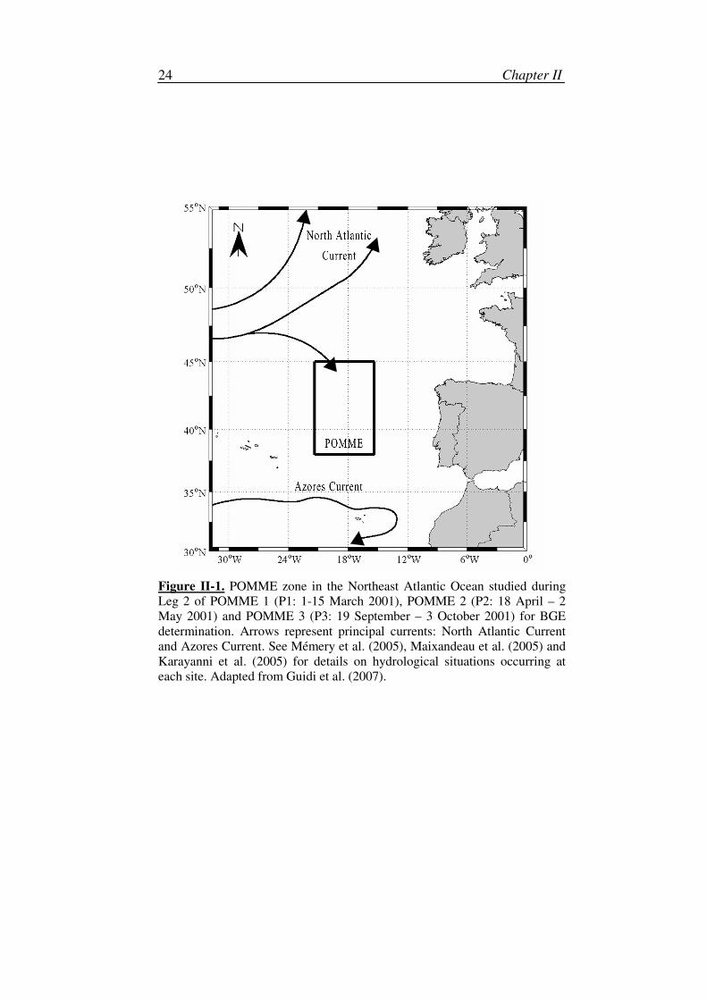
(POMME), seawater samples were collected in the Northeast Atlantic Ocean
(Figure II-1) over three seasons; winter (POMME 1; P1), spring (POMME 2;
P2) and summer (POMME 3; P3) 2001 (for further details on POMME and
on sampling techniques, see Mémery et al. 2005). It is beyond the scope of
this study to present a detailed protocol and mesoscale variability aspects,
and such data are available elsewhere (F. Van Wambeke et al. unpubl. data).
ii. General design
Seawater was collected from 3 depths (5, 200 and 400 m) using Niskin
bottles, then transferred immediately into large polycarbonate bottles without
tubing. The protocol for seawater collection and for minimising organic carbon
contamination is described in Sempéré et al. (2003). Following collection,
seawater was filtered, using a low vacuum (<50 mm Hg) through pre-combusted
(450°C, 6 hours) GF/F glass fibre filters in order to obtain bacterial seawater
cultures. This experimental design removes all DOC sources and all predators,
except for some viruses. A mean of 46 % of the in situ bacterial cells was passed
through the filters (F. Van Wambeke et al. unpubl. data). DOC was not
measured. However, we could not exclude the possibility that the filtration
process might induce some increase in DOC concentration and slightly modify
the bacterial activity, particularly in the deep samples, as in some cases specific
activity of bacteria after filtration increased compared to that in situ (F. Van
Wambeke et al. unpubl. data). The bulk incubation culture was then sub-sampled
by dispension into duplicate pre-combusted borosilicate bottles to determine BP
and bacterial abundance, and also into quadruplicate 125 ml Winkler bottles for
dissolved oxygen determination. The latter samples were fixed with Winkler
reagents, and measurements were made using an automated Winkler titration
system based on that described by Williams & Jenkinson (1982). Experimental
bottles were incubated in the dark in a temperature controlled room (± 1°C) over
the course of the experiments. Samples were sacrificed and analysed for BP and
dissolved oxygen using a time series of 0, 0.5, 1, 2, 5, 10 d. Consequently, we
must hypothesise that dynamics are identical in all bottles.
Chapter II 24
Figure II-1. POMME zone in the Northeast Atlantic Ocean studied during
Leg 2 of POMME 1 (P1: 1-15 March 2001), POMME 2 (P2: 18 April – 2
May 2001) and POMME 3 (P3: 19 September – 3 October 2001) for BGE
determination. Arrows represent principal currents: North Atlantic Current
and Azores Current. See Mémery et al. (2005), Maixandeau et al. (2005) and
Karayanni et al. (2005) for details on hydrological situations occurring at
each site. Adapted from Guidi et al. (2007).
Empirical model and in situ data 25
BP was calculated using the tritiated leucine method (Kirchman 1993). The
experimental estimation for BGE (BGEE) was calculated by integrating data
from time zero (t0) to the BP peak, which refers to the maximum BP value in the
time series, as follows:
2E
IBPBGE
OIBP t RQt
=∆
+∆
(II.1)
where IBP (µM C) was time-integrated BP from t0 to the BP peak with
trapezoidal integration of discrete data. The conversion factor of leucine-carbon
was 1.5 kg C mol-1
of leucine incorporated assuming an isotopic dilution of 1.
The oxygen consumption rate ∆O2/∆t (µM d-1
) was calculated assuming a linear
regression model for the decrease in dissolved oxygen concentration with time
(t). The respiratory quotient (RQ) was 0.8 (F. Van Wambeke et al. unpubl. data).
iii. DOC and bacterial biomass estimations
Initial bacterial biomass (BB) was determined by epifluorescence
microscopy after DAPI staining, assuming a carbon conversion factor (CCF)
of 20 fg C bacterium-1
(Lee & Fuhrman 1987). In order to estimate BB
increase, the IBP (derived from the leucine method, see equation II.1) was
added to this initial value of BB for computing the BB for all other time
points. Numerous hypotheses were made to assess DOC dynamics. Total
organic carbon (TOC) was measured using high temperature catalytic
oxidation (Sohrin & Sempéré 2005) on the in situ vertical profiles, but not for
the biodegradation experiments. Initial values of DOC were thus estimated as
the difference between in situ TOC and POC, which was deduced from total
particulate carbon (TPC) measurements obtained using an optical particle
counter (HIAC) (Merien 2003). As the proportion of DOC to TOC fraction
increases globally from 83 % at 5 m to 92 % at 200 m, we estimated that at
400 m DOC is close to TOC. We then assumed that initial DOC
concentration in the batches was close to in situ DOC concentration. Finally,
we estimated DOC concentrations over the course of the experiments on the
assumption that the quantity of DOC consumed over a short period, which
we assumed to be only L-DOC according to duration of experiments, is equal
to the sum of BB increase and CO2 produced over the same period, estimated
as:
∆ CO2 / ∆ t = - RQ x ∆ O2 /∆ t (II.2)
Chapter II 26
2. Monod (1942) model
The biodegradation model was set up on the basis of the following
assumptions. (1) There is no source of DOC in the cultures. (2) Bacteria are
the only organisms present (no flagellates and no virus) (these first 2
assumptions are likely to be valid, since only the growth phase, and thus a
short period of time, is considered). (3) L-DOC was the limiting factor on
bacterial growth, which is a reasonable assumption since nutrient
concentrations measured in water column profiles during the cruises were
sufficient to sustain bacterial growth in the experiments considered (NO3
concentrations ranged from 1.9 to 13.1 µM, except one value of 0.39 µM in
spring, and PO4 concentrations from 0.1 to 1.04 µM), except perhaps in
surface water in late summer where values were lower (from undetectable to
0.04 µM for NO3 and from 0.01 to 0.02 µM for PO4) (F. Van Wambeke et al.
unpubl. data). (4) We assumed that only the L-DOC fraction is consumed by
bacteria during the 10 d biodegradation experiments as well as in the model.
The Monod (1942) formula, which uses Michaelis-Menten kinetics, is
one of the simplest and most widely used models for describing the
interactions between 2 state variables, in this case bacterial C-biomass and
DOC. Note that in this model the disappearing DOC is instantaneously taken
up by bacteria and converted into C-biomass with a constant efficiency
(numerical bacterial growth efficiency, BGEN). Consequently, BGEN is
estimated using the model calibration and depends on the external limiting
food concentration.
max xV DOC BBdDOC
dt k DOC= −
+
(II.3)
max xN
V DOC BBdBBBGE
dt k DOC=
+
(II.4)
where BB is in µM C; DOC is concentration in µM C, with the assumption
that L-DOC is the limiting food resource and the only fraction of DOC
consumed; Vmax is the specific maximum assimilation rate in d-1
; and k is the
half-saturation constant for DOC in µM C.
The parameters (BGEN, Vmax and k) were estimated, for each experiment,
from all available DOC derived values and BB data. The parameter values
were thus estimated using a non-linear regression that uses the least-squares
Empirical model and in situ data 27
method. The calibration is performed for each experiment in order to
compare the parameters obtained from the model for different depths and
seasons. Nevertheless, it should be pointed out that DOC estimations are
representative of the total pool of DOC (L-DOC, semi-labile-DOC plus
refractory-DOC), whereas the model only simulates the decrease of L-DOC,
which constitutes the first and only fraction of DOC used by bacteria during
the 10 d biodegradation experiments. This does not affect the parameter
estimations, as semi-labile-DOC and refractory-DOC are supposed to be
constant and unaffected during these biodegradation experiments. Thus,
model parameters are representative of bacterial growth in batch cultures.
A sensitivity analysis was carried out to determine (1) which parameter
has the most influence on the dynamics, and (2) the validity of parameter
estimations according to experimental errors. First, the derivatives of the
model were calculated with respect to the parameters, the highest derivative
being the most influential parameter. This enables a quantitative comparison
of parameter sensitivity. We then analysed the robustness of the parameter
estimations with respect to the data. The measurement errors, the variability
of environmental forcing parameters on the measurements and the
assumptions made to assess DOC data may indeed indicate some variabilities
in the observations used to calibrate the model. We have estimated that the
sum of these variabilities was ≤ 30 %. For 1 experiment, 500 extra sets of
data were obtained by replacing each original data point in the course of the
experiments by its value multiplied by1 p± , where 3.0≤p and is a
random proportion that is uniformly distributed. Thus, ‘perturbed’ data
represent the value that a data point could have if we consider the accuracy of
the original data to be within the range of 70 to 100 %. We then estimated
parameters of the model for these 500 data sets using the same method as
those for data sets without perturbation. This procedure provides information
on the parameter distribution and on the robustness of the BGEN estimations.
3. Comparison of methods for BGE estimation
The present study calculated BGE in 2 ways: as BGEE and BGEN. Both
estimations implied assumptions about RQ and leucine-carbon conversion
factors, which are supposed to be constant and equal in the 2 BGE
estimations. The values of the BGEE may change with respect to BGEN
according to the method used to calculate the O2 utilisation rate, the
assumptions made to assess DOC data (as the CCF) and the integration time
considered. BGEE values are estimated using integrated data from t0 to the
BP peak and assuming a linear regression model for the decrease in dissolved
oxygen concentration, whereas values for BGEN are estimated using the
Chapter II 28
least-squares method between the outputs of the 2 state variables of the
model and the whole data set for each experiment. In order to compare the 2
methods, we calculated the relative quadratic distance (d) between BGEE and
BGEN for each biodegradation experiment by taking BGEE as reference:
E N
E
BGE BGEd
BGE
−
= (II.5)
If d is low (d << 1), the 2 methods of BGE estimation are thus considered
to be equivalent.
III. Results
1. Model calibration and simulation
We performed a calibration of the model with the data for each
experiment. The minimum distance between the model outputs and
experimental data are obtained from high values of Vmax and k in all
experiments. Consequently, DOC can be neglected in comparison to k, that is
k DOC k+ ≈ . Then, equations (II.3) and (II.4) can be approximated by the
following system (equations II.6 and II.7):
xdDOC
DOC BBdt
α= − (II.6)
xN
dBBBGE DOC BB
dtα= (II.7)
where maxV kα = in µM C-1
d-1
(II.8)
This simplified model can be solved analytically. Equations A.II.3 and
A.II.4 in Appendix II-A allow the removal of the integration step for the
calibration and simulation. The use of these equations enables analysis to be
performed faster and provides a more precise calibration.
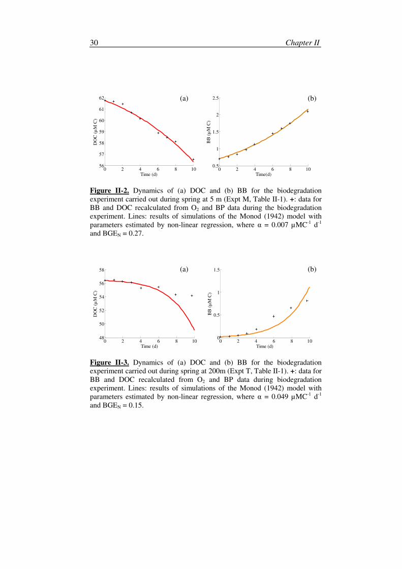
For most of the experiments (26 out of 36) the model (equations II.6 and
II.7) produces an accurate fit both qualitatively and quantitatively with
parameters α and BGEN (see Figure II-2). However, there is no agreement
between the model outputs and data in the case of the other 10 experiments
(see Figure II-3). Thus, these results have not been taken into account in the
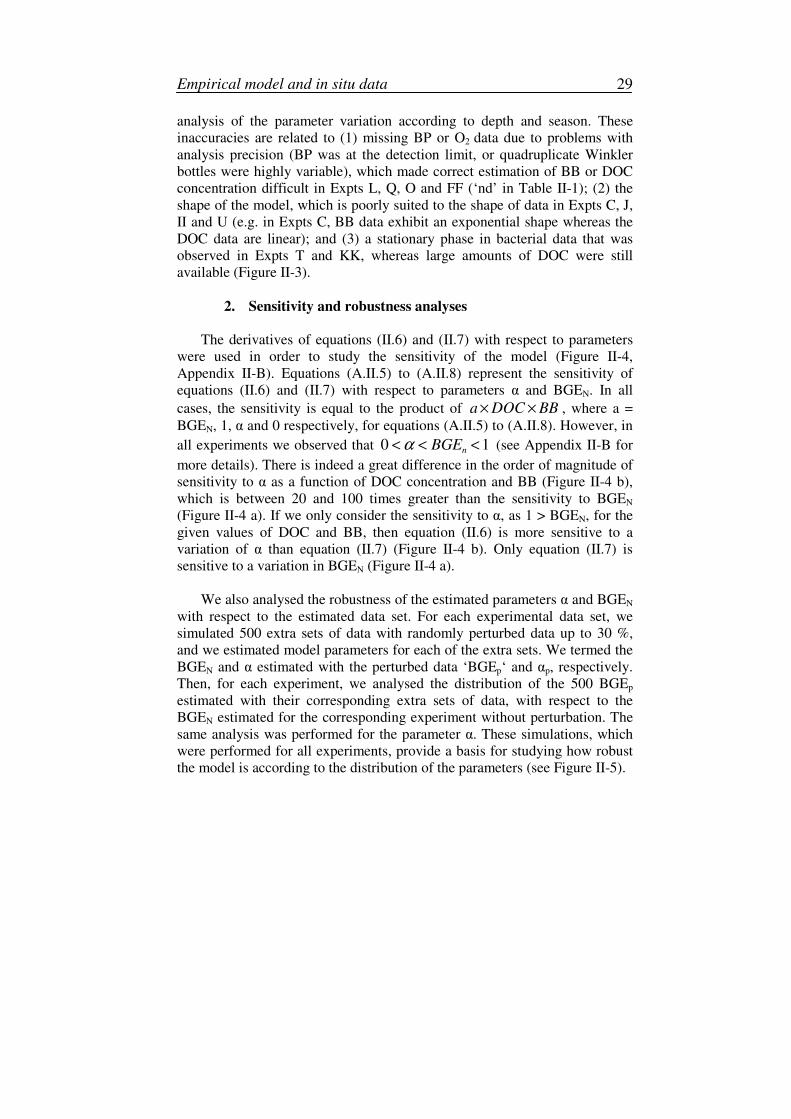
Empirical model and in situ data 29
analysis of the parameter variation according to depth and season. These
inaccuracies are related to (1) missing BP or O2 data due to problems with
analysis precision (BP was at the detection limit, or quadruplicate Winkler
bottles were highly variable), which made correct estimation of BB or DOC
concentration difficult in Expts L, Q, O and FF (‘nd’ in Table II-1); (2) the
shape of the model, which is poorly suited to the shape of data in Expts C, J,
II and U (e.g. in Expts C, BB data exhibit an exponential shape whereas the
DOC data are linear); and (3) a stationary phase in bacterial data that was
observed in Expts T and KK, whereas large amounts of DOC were still
available (Figure II-3).
2. Sensitivity and robustness analyses
The derivatives of equations (II.6) and (II.7) with respect to parameters
were used in order to study the sensitivity of the model (Figure II-4,
Appendix II-B). Equations (A.II.5) to (A.II.8) represent the sensitivity of
equations (II.6) and (II.7) with respect to parameters α and BGEN. In all
cases, the sensitivity is equal to the product of a DOC BB× × , where a =
BGEN, 1, α and 0 respectively, for equations (A.II.5) to (A.II.8). However, in
all experiments we observed that 0 1nBGEα< < < (see Appendix II-B for
more details). There is indeed a great difference in the order of magnitude of
sensitivity to α as a function of DOC concentration and BB (Figure II-4 b),
which is between 20 and 100 times greater than the sensitivity to BGEN
(Figure II-4 a). If we only consider the sensitivity to α, as 1 > BGEN, for the
given values of DOC and BB, then equation (II.6) is more sensitive to a
variation of α than equation (II.7) (Figure II-4 b). Only equation (II.7) is
sensitive to a variation in BGEN (Figure II-4 a).
We also analysed the robustness of the estimated parameters α and BGEN
with respect to the estimated data set. For each experimental data set, we
simulated 500 extra sets of data with randomly perturbed data up to 30 %,
and we estimated model parameters for each of the extra sets. We termed the
BGEN and α estimated with the perturbed data ‘BGEp‘ and αp, respectively.
Then, for each experiment, we analysed the distribution of the 500 BGEp
estimated with their corresponding extra sets of data, with respect to the
BGEN estimated for the corresponding experiment without perturbation. The
same analysis was performed for the parameter α. These simulations, which
were performed for all experiments, provide a basis for studying how robust
the model is according to the distribution of the parameters (see Figure II-5).
Chapter II 30
0 2 4 6 8 1056
57
58
59
60
61
62
Time (d)
DO
C (
µM
C)
0 2 4 6 8 100.5
1
1.5
2
2.5
Time(d)
BB
(µ
M C
)
Figure II-2. Dynamics of (a) DOC and (b) BB for the biodegradation
experiment carried out during spring at 5 m (Expt M, Table II-1). +: data for
BB and DOC recalculated from O2 and BP data during the biodegradation
experiment. Lines: results of simulations of the Monod (1942) model with
parameters estimated by non-linear regression, where α = 0.007 µMC-1
d-1
and BGEN = 0.27.
0 2 4 6 8 1048
50
52
54
56
58
Time (d)
DO
C (
µM
C)
0 2 4 6 8 100
0.5
1
1.5
Time (d)
BB
(µ
M C
)
Figure II-3. Dynamics of (a) DOC and (b) BB for the biodegradation
experiment carried out during spring at 200m (Expt T, Table II-1). +: data for
BB and DOC recalculated from O2 and BP data during biodegradation
experiment. Lines: results of simulations of the Monod (1942) model with
parameters estimated by non-linear regression, where α = 0.049 µMC-1
d-1
and BGEN = 0.15.
(a)
(a)
(b)
(b)
Empirical model and in situ data 31
In all experiments, the distribution of parameters following perturbation
follows a unimodal low, and parameters estimated without perturbation are
within or close to the modal class. In each experiment, 90 to 100 % of the
500 perturbation simulations give rise to a BGEp< 0.4, indicating a weak
distribution of BGEp. Moreover, > 50 % of the perturbation experiments give
rise to: BGEN - 0.1 < BGEp < BGEN + 0.1. A small percentage of the results
gives a BGEp close to 1 (not shown). This result could be related to the
scattering of DOC data caused by the perturbation; indeed, this scattering
does not give a satisfactory model fit and the calibration method produces a
curve with a very small αp. This indicates that the BB data, where the level of
scattering is lower and thus well fitted, needs to be fitted using a very high
value of BGEp in order to balance the weak αp. The values of α without
perturbation are in the middle of the distribution and the highest αp is double
that of α without perturbation.
3. Parameters
For each experiment, values of α and BGEN obtained by the
parameterisation of the model are presented in relation to the BGEE
calculated experimentally from O2 and BP data (Tables II 1-2). For some
experiments, there were no results because of experimental problems (nd in
Table II-1). BGEE ranged from 0.01 to 0.48, whereas α and BGEN ranged
from 0.006 to 0.097 µM C-1
d-1
and from 0.04 to 0.41, respectively. BGE
values were also averaged at each depth for a given season, at each season for
a given depth and at each depth for the whole year (Table II-2). By
calculating these means, the results where simulations were not possible or
seemed inaccurate were excluded (see ‘Results; Model calibration and
simulation’). As the number of results for a given depth and season were
small (n = 4 in general) and some were not taken into account in means, the
standard deviations increase rapidly when we remove 1 or 2 results (n = 3
and 2, respectively, Table II-2).
The relative quadratic distances d between BGEE and BGEN range from
0.07 to 12.00 (Figure II-6). All distances, except 6 out of 26, have d < 0.5 and
all except 3 have d < 1, which suggests that the 2 methods of BGE estimation
are quantitatively equivalent.
The results indicate that mean BGEN decreases from the surface (5 m) to
deeper waters (200 and 400 m) in spring and summer, whereas there is no
significant relationship with depth in winter (Table II-2). If we consider the
annual means, we observe a decrease in BGEN with depth. However, the
mean BGEN varies according to season in the surface layer with a minimum
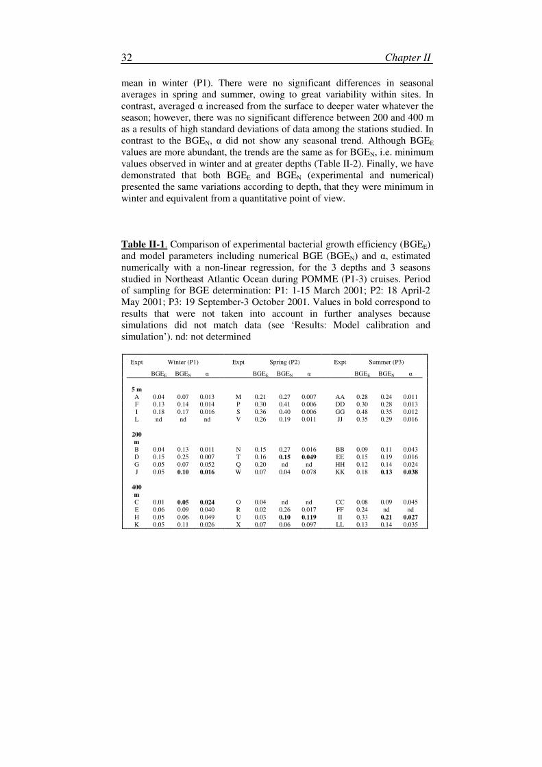
Chapter II 32
mean in winter (P1). There were no significant differences in seasonal
averages in spring and summer, owing to great variability within sites. In
contrast, averaged α increased from the surface to deeper water whatever the
season; however, there was no significant difference between 200 and 400 m
as a results of high standard deviations of data among the stations studied. In
contrast to the BGEN, α did not show any seasonal trend. Although BGEE
values are more abundant, the trends are the same as for BGEN, i.e. minimum
values observed in winter and at greater depths (Table II-2). Finally, we have
demonstrated that both BGEE and BGEN (experimental and numerical)
presented the same variations according to depth, that they were minimum in
winter and equivalent from a quantitative point of view.
Table II-1. Comparison of experimental bacterial growth efficiency (BGEE)
and model parameters including numerical BGE (BGEN) and α, estimated
numerically with a non-linear regression, for the 3 depths and 3 seasons
studied in Northeast Atlantic Ocean during POMME (P1-3) cruises. Period
of sampling for BGE determination: P1: 1-15 March 2001; P2: 18 April-2
May 2001; P3: 19 September-3 October 2001. Values in bold correspond to
results that were not taken into account in further analyses because
simulations did not match data (see ‘Results: Model calibration and
simulation’). nd: not determined
Winter (P1)
Expt Spring (P2)
Expt Summer (P3)
Expt
BGEE BGEN α BGEE BGEN α BGEE BGEN α
5 m
A 0.04 0.07 0.013 M 0.21 0.27 0.007 AA 0.28 0.24 0.011
F 0.13 0.14 0.014 P 0.30 0.41 0.006 DD 0.30 0.28 0.013
I 0.18 0.17 0.016 S 0.36 0.40 0.006 GG 0.48 0.35 0.012
L nd nd nd V 0.26 0.19 0.011 JJ 0.35 0.29 0.016
200
m
B 0.04 0.13 0.011 N 0.15 0.27 0.016 BB 0.09 0.11 0.043
D 0.15 0.25 0.007 T 0.16 0.15 0.049 EE 0.15 0.19 0.016
G 0.05 0.07 0.052 Q 0.20 nd nd HH 0.12 0.14 0.024
J 0.05 0.10 0.016 W 0.07 0.04 0.078 KK 0.18 0.13 0.038
400
m
C 0.01 0.05 0.024 O 0.04 nd nd CC 0.08 0.09 0.045
E 0.06 0.09 0.040 R 0.02 0.26 0.017 FF 0.24 nd nd
H 0.05 0.06 0.049 U 0.03 0.10 0.119 II 0.33 0.21 0.027
K 0.05 0.11 0.026 X 0.07 0.06 0.097 LL 0.13 0.14 0.035
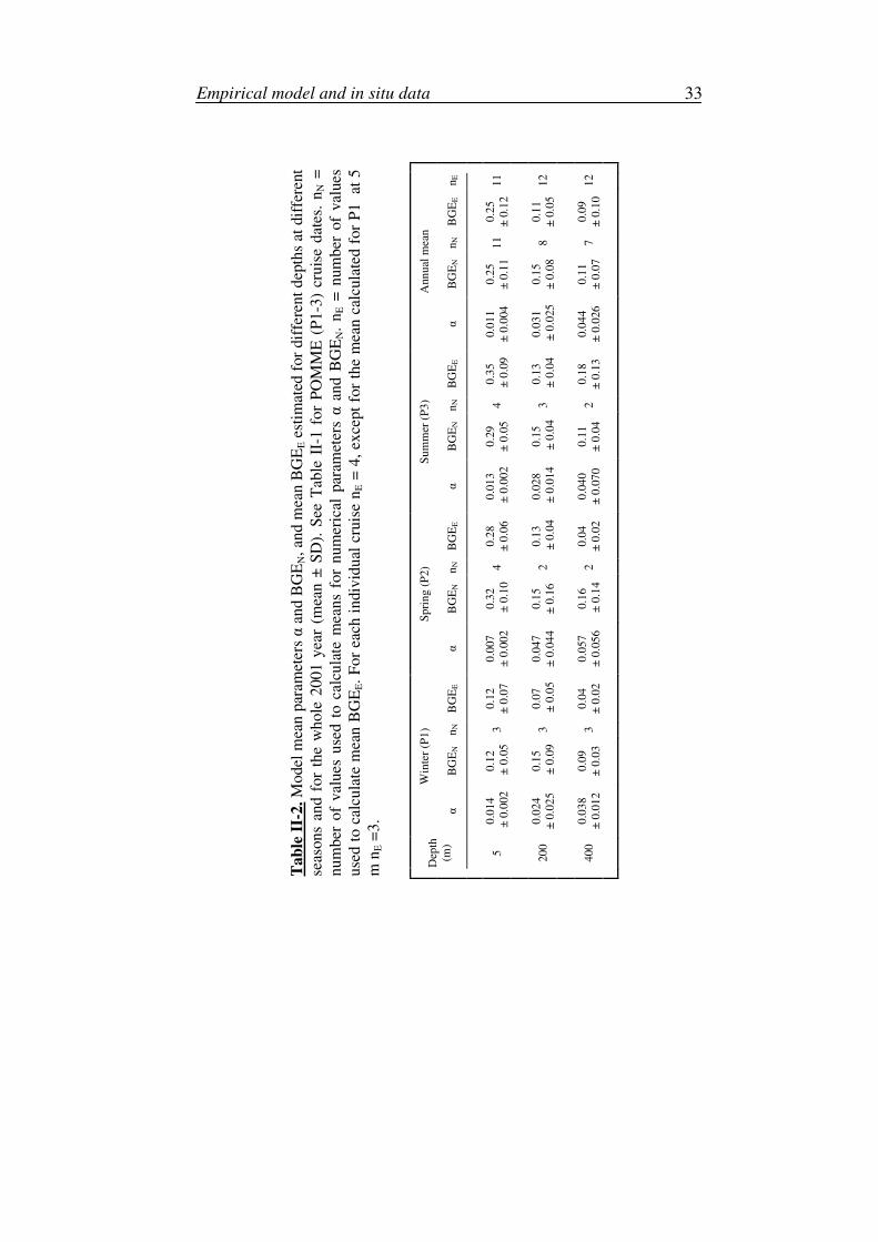
Empirical model and in situ data 33
Ta
ble
II-
2.
Mo
del
mea
n p
aram
eter
s α
an
d B
GE
N,
and
mea
n B
GE
E e
stim
ated
for
dif
fere
nt
dep
ths
at d
iffe
rent
seas
on
s an
d f
or
the
wh
ole
20
01
yea
r (m
ean
± S
D).
See
Tab
le I
I-1
fo
r P
OM
ME
(P
1-3
) cr
uis
e d
ates
. n
N =
nu
mb
er o
f v
alu
es u
sed t
o c
alcu
late
mea
ns
for
nu
mer
ical
par
amet
ers α
an
d B
GE
N.
nE =
num
ber
of
val
ues
use
d t
o c
alcu
late
mea
n B
GE
E.
Fo
r ea
ch i
ndiv
idu
al c
ruis
e n
E =
4,
exce
pt
for
the
mea
n c
alcu
late
d f
or
P1
at
5
m n
E =
3.
Win
ter
(P1
) S
pri
ng (
P2)
Su
mm
er (
P3
) A
nn
ual
mea
n
Dep
th
(m)
α
BG
EN
nN
BG
EE
α
BG
EN
nN
BG
EE
α
BG
EN
nN
BG
EE
α
BG
EN
nN
BG
EE
nE
5
0
.01
4
± 0
.002
0.1
2
± 0
.05
3
0.1
2
± 0
.07
0.0
07
± 0
.00
2
0.3
2
± 0
.10
4
0.2
8
± 0
.06
0.0
13
± 0
.00
2
0.2
9
± 0
.05
4
0
.35
± 0
.09
0.0
11
± 0
.004
0.2
5
± 0
.11
1
1
0.2
5
± 0
.12
1
1
20
0
0.0
24
± 0
.02
5
0.1
5
± 0
.09
3
0.0
7
± 0
.05
0.0
47
± 0
.04
4
0.1
5
± 0
.16
2
0.1
3
± 0
.04
0.0
28
± 0
.01
4
0.1
5
± 0
.04
3
0
.13
± 0
.04
0.0
31
± 0
.025
0.1
5
± 0
.08
8
0.1
1
± 0
.05
1
2
40
0
0.0
38
± 0
.01
2
0.0
9
± 0
.03
3
0.0
4
± 0
.02
0.0
57
± 0
.05
6
0.1
6
± 0
.14
2
0.0
4
± 0
.02
0.0
40
± 0
.07
0
0.1
1
± 0
.04
2
0
.18
± 0
.13
0.0
44
± 0
.026
0.1
1
± 0
.07
7
0.0
9
± 0
.10
1
2
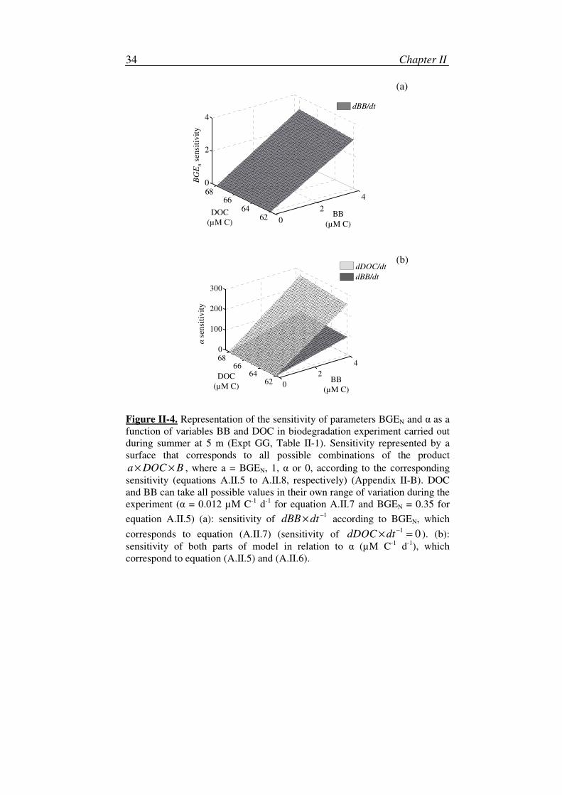
Chapter II 34
0
2
4
6264
66680
2
4
dBB/dt
BB
(µM C)
DOC
(µM C)
BG
En
sen
siti
vit
y
0
2
4
6264
66680
100
200
300
dDOC/dt
dBB/dt
BB
(µM C)
DOC
(µM C)
αse
nsi
tiv
ity
Figure II-4. Representation of the sensitivity of parameters BGEN and α as a
function of variables BB and DOC in biodegradation experiment carried out
during summer at 5 m (Expt GG, Table II-1). Sensitivity represented by a
surface that corresponds to all possible combinations of the product
a DOC B× × , where a = BGEN, 1, α or 0, according to the corresponding
sensitivity (equations A.II.5 to A.II.8, respectively) (Appendix II-B). DOC
and BB can take all possible values in their own range of variation during the
experiment (α = 0.012 µM C-1
d-1
for equation A.II.7 and BGEN = 0.35 for
equation A.II.5) (a): sensitivity of 1
dBB dt−
× according to BGEN, which
corresponds to equation (A.II.7) (sensitivity of 1 0dDOC dt
−
× = ). (b):
sensitivity of both parts of model in relation to α (µM C-1
d-1
), which
correspond to equation (A.II.5) and (A.II.6).
(a)
(b)
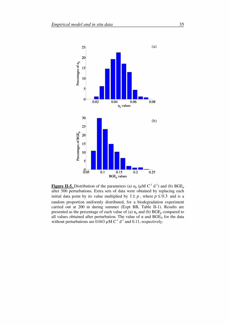
Empirical model and in situ data 35
0.02 0.04 0.06 0.080
5
10
15
20
25
αp values
Per
centa
ges
ofα
p
0.02 0.04 0.06 0.080
5
10
15
20
25
αp values
Per
centa
ges
ofα
p
0.05 0.1 0.15 0.2 0.250
5
10
15
20
25
30
BGEp values
Per
centa
ges
of
BG
Ep
0.05 0.1 0.15 0.2 0.250
5
10
15
20
25
30
BGEp values
Per
centa
ges
of
BG
Ep
Figure II-5. Distribution of the parameters (a) αp (µM C-1
d-1
) and (b) BGEp
after 500 perturbations. Extra sets of data were obtained by replacing each
initial data point by its value multiplied by p±1 , where 3.0≤p and is a
random proportion uniformly distributed, for a biodegradation experiment
carried out at 200 m during summer (Expt BB, Table II-1). Results are
presented as the percentage of each value of (a) αp and (b) BGEp compared to
all values obtained after perturbation. The value of α and BGEN for the data
without perturbations are 0.043 µM C-1
d-1
and 0.11, respectively.
(a)
(b)
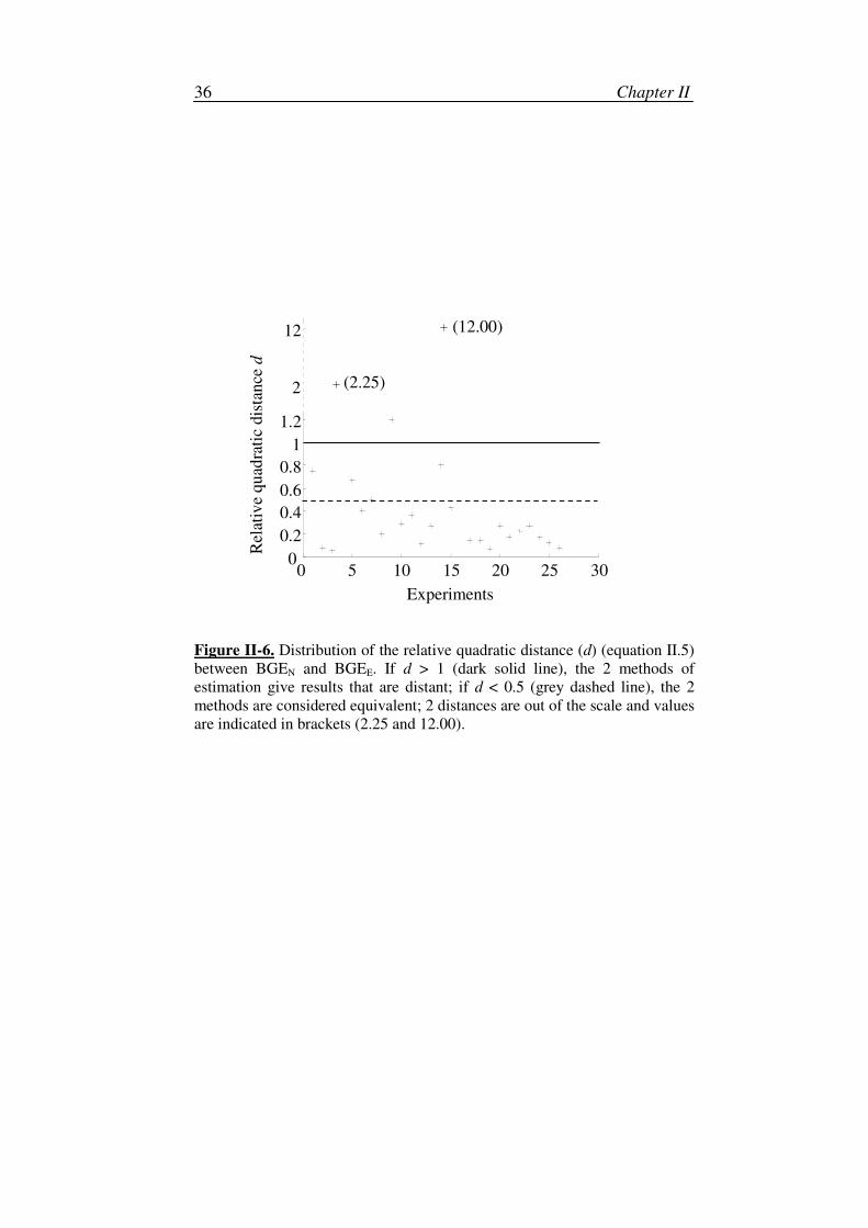
Chapter II 36
0 5 10 15 20 25 300
0.2
0.4
0.6
0.8
1
1.2
2
12
Experiments
Rel
ativ
e quad
rati
cdis
tance
d
(2.25)
(12.00)
Figure II-6. Distribution of the relative quadratic distance (d) (equation II.5)
between BGEN and BGEE. If d > 1 (dark solid line), the 2 methods of
estimation give results that are distant; if d < 0.5 (grey dashed line), the 2
methods are considered equivalent; 2 distances are out of the scale and values
are indicated in brackets (2.25 and 12.00).
Empirical model and in situ data 37
IV. Discussion
1. Analysis of model results
The model fits the data in almost all simulations. However, in some
cases, we observed that the model did not match the experimental data. For
example, the experimental dynamics of BB seemed to reach a stationary
phase even though there was still a significant concentration of DOC
(remaining 47 and 54 µM C for Expts KK and T, respectively) (Table II-1,
Figure II-3). The stationary phases observed in these experiments are likely
to be due to a complete exhaustion of L-DOC, because the remaining DOC in
the batch is close to that found in deep waters (40 – 50 µM C) (Sohrin &
Sempéré 2005) and in situ nutrient concentrations were sufficient to avoid
limitation (see ‘Materials and Methods; Monod (1942) model’). This
remaining DOC is represented by semi-labile and refractory-DOC poorly
assimilated by bacteria and not represented in the model, and thus the
bacterial stationary phase cannot be simulated.
Except for these biodegradation experiments, the sensitivity analysis has
demonstrated that the Monod (1942) model is more sensitive to a variation of
maxV k ratio than to BGEN, indicating that the best estimations of both
parameters require high precision in α values. Our results also demonstrate
that a perturbation comprised up to 30 % of total variation in data affects the
parameter estimations within a reasonable range: parameters estimated
without perturbation are always within or close to the modal class; the
distributions of parameters with perturbed experimental data are not very
large around the parameters estimated without perturbation; and >50 % of the
perturbation simulations give rise to: BGEN - 0.1 < BGEp < BGEN + 0.1. As
such perturbations only influence the estimation of both parameters to a low
order of magnitude, we can be sure that the parameters estimated without
perturbation are reliable. However, for some of these perturbations we
obtained BGEp values close to 1. For these perturbations, the model does not
match in the case of very small L-DOC variations (e.g. owing to a low signal-
to-noise ratio of variations of O2 data). As the relative quadratic distances d
for most experiments are ≤ 0.5, our estimations of BGEN are close to the
classical estimations of equation (II.1) (BGEE). Moreover, we have
demonstrated that the tendencies are the same when considering the 2 BGE
(BGEE and BGEN). Consequently, the overall analysis of the model
(qualitative and quantitative comparisons with experimental parameters,
sensitivity and robustness analyses) shows that our numerical method of
BGE estimation is well suited.
Chapter II 38
2. Biological analysis
The parameter values, revealed by the calibration of the model, have
shown a range of BGEN values below 0.5 (0.04 to 0.41, Table II-1) which is
commonly observed in diverse aquatic habitats (del Giorgio & Cole 1998).
The annual mean and standard deviations of BGEN at 5 m (0.25 ± 0.11) are
consistent with published data for the Gulf of Mexico (Pomeroy et al. 1995,
Jorgensen et al. 1999), Sargasso Sea (Carlson & Ducklow 1996) and the
Atlantic Jet in the Mediterranean Sea (Sempéré et al. 2003). BGEN at 5 m
was greater than at 200 and 400 m, and minimum values were observed in
the winter as was also the case in the surface layer of the North Sea
(Reinthaler & Herndl 2005). In contrast, minimum values of α were reached
at 5 m and no trend emerged with season. The fraction of refractory-DOC
increases with depth (Carlson 2002). Bacteria probably consume, in addition
to L-DOC, some semi-labile and refractory organic compounds. Therefore,
the fraction of assimilated L-DOC probably decreases with depth, and it is
conceivable that BGE decreases with depth. As α is the ratio between
maxV and k, the increase in α reflects an increase in bacterial affinity for
substrate with increasing depth (decrease of k) and/or better specific
maximum assimilation rates (increase of maxV ). These results suggest that the
more refractory bulk DOC (representative of those observed below the
productive layer, i.e. 200 m) (Sohrin & Sempéré 2005), as well as probable
patchy distribution of L-DOC in deep waters, would explain lower BGE,
higher affinity to the substrate and/or higher specific maximum assimilation
rates.
3. Experimental problems
The data needed for the calibration were not directly measured. Patterns
of change over time of DOC estimations are based on BP and BR, which
were themselves estimated from indirect measurements (leucine
incorporation and O2 variations). Hence, conversion factors (leucine to
carbon, RQ) must be applied. The latter is not constant as bacteria can change
their RQ (Kooijman 2000) according to changes in the quality and quantity
of the substrate over the course of the experiments. However, the changes
over time of these conversion factors has no influence on the comparison of
BGE, as the same values were used in both cases (BGEE and BGEN) and the
influence of these factors is discussed elsewhere (F. Van Wambeke et al.
unpubl. data). Moreover, these changes of conversion factors over time have
to be proven experimentally in order to be taken into account. It further
results that the estimations of DOC concentrations may not be accurate and
Empirical model and in situ data 39
representative of the real variation in DOC in the experiments. Direct
measurements of DOC would be more appropriate, but there is, for instance,
no protocol which is sufficiently sensitive for oligotrophic waters.
Nevertheless, even if data vary by up to 30 % of the values without
perturbation, the method of parameterisation is well suited. Consequently,
estimated parameters are reliable. We have also assumed that the DOC
concentration at a given time equals the initial DOC, minus the sum of CO2
respired and BB produced. However, this hypothesis would be accurate only
if the system behaves as a Monod (1942) model, i.e. if growth and respiration
depend directly on the external concentration of the substrate. The presence
of an internal carbon reservoir in bacteria (Ducklow & Carlson 1992,
Cherrier et al. 1996) may indeed induce a time lag between assimilation and
growth and/or respiration, which has not been taken into account in
estimations of the data sets needed for the calibration of the model.
Another bias is the difficulty in placing these results within a natural
context. For example, the presence of viruses, which may induce a decrease
in BGE and an increase in the growth rate of uninfected cells, cannot be ruled
out (Middelboe et al. 1996). These are not represented in the model whereas
they may in fact reduce bacterial abundance. Although great care was taken
during filtration (Yoro et al. 1999), this process is likely to induce an increase
in DOC due to particle breakdown (Carlson et al. 1999, Ducklow et al. 1999).
However, increases in specific leucine incorporation rates at t0 from
biodegradation experiments compared to their respective values in situ values
occurred in less than half of the experiments (F. Van Wambeke et al. unpubl.
data). The 10 d incubation experiments could also enable bacteria to use
more refractory organic matter, thus lowering natural BGE (del Giorgio &
Cole 1998, Carlson et al. 1999). Although these analytical biases are difficult
to quantify, they should be kept in mind for comparisons and further
interpretation.
4. Improvement of biogeochemical models
We have demonstrated using the Monod (1942) model that (1)
parameters BGEN and α are dependent on depth, and (2) BGEN varies
according to season, especially in the surface layer, in the Northeast Atlantic
Ocean. Consequently, the use of a constant BGEN and α in 1-dimensional
biogeochemical models (Anderson & Williams 1999, Lancelot et al. 2002)
may not be appropriate. It is necessary to find a better method to simulate the
uptake of organic matter by bacteria, for example by expressing BGEN and α
as a function of depth, since the availability of L-DOC varies with depth. The
seasonal changes in BGEN should also be described, for example with
Chapter II 40
temperature. Other environmental factors such as the composition in organic
nutrients, phages and physiological conditions may affect the BGE (Cajal-
Medrano & Maske 2005). Moreover, BGE values could influence the
existence and competition of bacterial communities living on distinct
substrates (Miki & Yamamura 2005).
The time lag between assimilation of the substrate, respiration and
growth may require mathematical descriptions for each of these kinetics.
Some models that use variable BGEN, such as the Droop (1968) model, take
into account internal variable carbon storage (Grover 1991). In the case of
DOC uptake by bacteria, this model allows bacteria to absorb the substrate in
part of the cell, referred to here as the quota. Then, carbon stored in the quota
will be allocated for different bacterial processes including maintenance and
growth. In contrast to the Monod (1942) model, the Droop (1968) model also
allows bacteria to survive during a starvation period, and requires
differentiation of assimilation and growth processes. These assumptions give
a better understanding of the interaction between DOC and bacteria in
biogeochemical models (Vichi et al. 2003) and allow a variable BGE to be
considered as BGE dBB dDOC= .
Previous studies indicate that bacteria supplied with phosphorus are able
to store organic carbon, without dividing, thereby maintaining a higher BGE
(Zweifel et al. 1993). The assumption of carbon storage has also been
proposed with observation of a non-coupling between (1) the use of DOC
and (2) BP and BR (Ducklow & Carlson 1992, Cherrier et al. 1996). It is also
important to take into consideration the metabolic energy used for
maintenance processes, i.e. processes that do not produce new biomass but
maintain cell integrity, in bacterial modelling (Cajal-Medrano & Maske
1999, 2005). Some authors indicate that the addition of reserves and the
maintenance in a Monod (1942) model is necessary in order to obtain the
bacterial dynamics in chemostats (Kooi & Kooijman 1994, Kooijman 2000).
We have to test such models using data from biodegradation experiments and
study the effects on biogeochemical models. In the first case, the substrate is
constant in the cultures but there are changes in the populations, which
proliferate or dominate in cultures; in contrast, in the second case, there are
changes in the availability of the substrate over the course of the experiment.
Consequently, the description of the interactions between bacteria and DOC
in biogeochemical models should be reviewed in order to include some
fundamental mechanisms such as the use of reserves and the maintenance
processes.
Empirical model and in situ data 41
V. Conclusion
We have shown that Monod-type modelling constitutes a fast and cheap
method to estimate BGE from bacterial biodegradation experiments (DOC
and BB data). This model is not very sensitive to variation in parameters and
is robust with regard to experimental errors. However, in order to obtain BGE
estimations close to the natural BGE, accurate measured experimental data
are required. Moreover, more experiments are needed to observe the decrease
in BGE and increase in α with depth with the dynamics of both state
variables recorded over different seasons: rigid sampling with regard to depth
and time with replicates is essential. An experimental process using the most
precise measurements available is crucial for the calibration and validation of
any model. Moreover, DOC data is necessary to validate our approach and
thus our results. The introduction of BGE as a function of depth and
temperature in the model of Anderson & Williams (1999) could prove to be
the way forward. Nevertheless, the Monod (1942) model was designed for a
system in steady-state in the natural environment; however, there are always
perturbations and the steady-state condition is rare. Consequently, models
using time variable assimilation rate and BGE such as Droop (1968) and
Dynamic Energy Budget models (Kooijman 2000) should be investigated
more thoroughly in order to reproduce the observations more accurately.
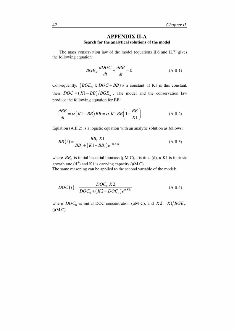
Chapter II 42
APPENDIX II-A Search for the analytical solutions of the model
The mass conservation law of the model (equations II.6 and II.7) gives
the following equation:
0N
dDOC dBBBGE
dt dt+ = (A.II.1)
Consequently, ( )xNBGE DOC BB+ is a constant. If K1 is this constant,
then ( )1 NDOC K BB BGE= − . The model and the conservation law
produce the following equation for BB:
( )1 1 11
dBB BBK BB BB K BB
dt Kα α
= − = −
(A.II.2)
Equation (A.II.2) is a logistic equation with an analytic solution as follows:
( )( )
0
1
0 0
1
1 K t
BB KBB t
BB K BB eα−
=
+ −
(A.II.3)
where 0BB is initial bacterial biomass (µM C), t is time (d), α K1 is intrinsic
growth rate (d-1
) and K1 is carrying capacity (µM C)
The same reasoning can be applied to the second variable of the model:
( )( )
0
1
0 0
2
2 K t
DOC KDOC t
DOC K DOC eα
=
+ −
(A.II.4)
where 0DOC is initial DOC concentration (µM C), and 2 1N
K K BGE=
(µM C).
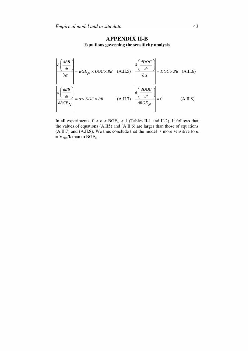
Empirical model and in situ data 43
APPENDIX II-B Equations governing the sensitivity analysis
dBB
dtBGE DOC BB
Nα
∂
= × ×
∂
(A.II.5)
dDOC
dtDOC BB
α
∂
= ×
∂
(A.II.6)
dBB
dtDOC BB
BGEN
α
∂
= × ×
∂
(A.II.7) 0
dDOC
dt
BGEN
∂
=
∂
(A.II.8)
In all experiments, 0 < α < BGEN < 1 (Tables II-1 and II-2). It follows that
the values of equations (A.II5) and (A.II.6) are larger than those of equations
(A.II.7) and (A.II.8). We thus conclude that the model is more sensitive to α
= Vmax/k than to BGEN.

44
45
CHAPTER III
Biodegradation experiments in
variable environments: substrate
pulses and impact on growth
efficiencies
Chapter III 46
Eichinger M, Sempéré R, Poggiale JC, Grégori G, Charrière B
and Lefèvre D (In prep)
Abstract
Biodegradation experiments are often carried out in batch cultures to
determine bacterial properties such as the bacterial growth efficiency (BGE).
We conducted biodegradation experiments with a unique bacterial strain and
a unique carbon limiting substrate in order to study bacterial activities in two
kinds of experimental environments. The only difference between these two
experiments was the substrate regime. In the first experiment, the substrate
was periodically pulsed in the culture. The same concentration was added at
each pulse. In the second experiment all the substrate was added in the
beginning of the experiment, the total amount of substrate introduced being
the same in both experiments. These experiments first allowed pointing out
key processes of bacterial growth and degradation activities. We
demonstrated that the various bacterial measurements co-vary in both
experiments. However, the specific carbon content varied during the
experiments. We also observed a production of refractory material during the
time course of the experiments. The respiration measurement allowed
identifying maintenance process as well as the instantaneous response to the
pulse addition. Then, three models were calibrated on the data sets. Two
models, the Monod and the Marr-Pirt models, are empiric. The third model
originated from the Dynamic Energy Budget (DEB) theory and was
especially constructed for the pulse experiment due to the presence of
starvation periods. Each of these models allowed the estimation of the BGE.
The BGE was also calculated experimentally directly from the data sets. It
results that the BGE, what else the method used, was always higher for the
pulse than for the batch experiment. It seems that bacteria adapt their
metabolism to respond to environmental perturbations, for example by
adapting their assimilation or growth efficiencies.
Biodegradation experiments in variable environment 47
I. Introduction
Dissolved organic carbon (DOC) represents one of the largest active
organic carbon reservoirs in the biosphere (Hedges 1992, Amon & Benner
1996). It is widely accepted that DOC represents a dynamic component in the
interaction between geosphere, hydrosphere and biosphere and as such has
the potential to influence the global carbon cycle and climate change
(Farrington 1992). Numerous processes are responsible of DOC production
such as release by phytoplankton, egestion, excretion and sloppy feeding
from grazers and cellular lysis generated by viruses (Nagata 2000). On the
other hand, heterotrophic bacteria are considered as the major consumers and
remineralisers of DOC in the ocean (Pomeroy 1974, Williams 2000).
According to bacterial reactivity, DOC is usually fractionated into three
pools: the refractory DOC (R-DOC) which turns over on the time scale of
millennia and that accumulates in ocean, semi-labile DOC (SL-DOC) which
turns over on the scale of months to years and labile DOC (L-DOC) which
turns over on the scale of hours to days (Williams & Druffel 1987, Carlson &
Ducklow 1995, Hansell et al. 1995, Carlson & Ducklow 1996, Nagata 2000,
Carlson 2002). The SL-DOC and R-DOC concentrations are usually
determined by examining DOC profiles throughout the water column,
assuming that in deep-water (> 1000 m) only R-DOC occurs and that the
water column has the same R-DOC concentration (Carlson & Ducklow 1995,
Wheeler et al. 1996, Wiebinga & de Baar 1998, Sohrin & Sempéré 2005).
The L-DOC component can be studied by measuring the bacterial DOC
consumption in biological assays (Carlson & Ducklow 1996, Cherrier et al.
1996, Sempéré et al. 1998, Carlson et al. 1999). The fraction of DOC that is
transferred to higher trophic levels by bacteria is estimated by the assessment
of the L-DOC utilisation in biodegradation experiments. These experiments
must be carried out by forcing an uncoupling both of DOC production from
consumption, and of bacterial production from bacterivory (Carlson &
Ducklow 1996). Consequently, experiments are generally performed either
by isolating bacteria from primary producers and grazers by filtering
seawater if experiments result from in situ sampling, or by working on mono-
species strains of bacteria in pure cultures.
Due to physical, chemical and biological processes (Carlson & Ducklow
1995, Carlson et al. 2004, La Ferla et al. 2005) and to the decoupling between
the production and consumption terms (Hansell et al. 1995, Carlson et al.
2002), the DOC concentration fluctuates spatially and temporally in oceanic
ecosystems. Relatively weak temporal variations in the dynamics of the water
column may have a great impact on the functioning of the pelagic system
Chapter III 48
(González et al. 2002). Thus, it is crucial to study the responses of microbial
communities to intermittent or transient forms of reactive DOC (Cherrier &
Bauer 2004). The fluctuation of DOC availability varies spatially, from the
presence of microzones containing elevated substrate concentration
(Williams 2000) to the large scale as the nearshore zone influenced by
upwelling events (Mcmanus & Peterson 1988). Temporal fluctuations range
from the daily cycle due to highest phytoplankton production during daylight
(Coffin et al. 1993) to the seasonal time scale for example due to the release
of DOC during a phytoplankton bloom (Miki & Yamamura 2005a, Grossart
& Simon 2007). However, experimental studies are generally carried out with
natural seawater by adding for example a fresh plankton-derived DOC pulse
in the start of the experiment (Cherrier & Bauer 2004). Even if this
experimental setup allows alleviating problems due to DOC production and
bacterial grazing, it still presents problems due to DOC measurement
accuracy, and especially the problem of the assessment of DOC lability.
Another difficulty in the interpretation of the results comes from bacterial
activity: is the bacterial count or biomass increase related to the DOC
utilisation? The final conclusions from results of this experimental design are
based on lots of assumptions.
The bacterial growth efficiency (BGE) is a widely used factor that
enables the estimation of the carbon flows through the bacterioplankton.
BGE indicates the proportion of the dissolved organic matter (DOM) that is
made available by the bacteria as particulate organic matter (POM) and that
may be consumed by the higher trophic levels (Cajal-Medrano & Maske
2005). It thus has a profound effect on the marine organic carbon cycle (del
Giorgio & Cole 1998, del Giorgio & Duarte 2002). BGE is generally
experimentally determined from bacterial production (BP) and bacterial
respiration (BR) measurements, or from BP and bacterial carbon demand
(BCD) according to the following formula: BGE = BP/BCD where BCD =
BP+BR (del Giorgio & Cole 1998, Sempéré et al. 1998, Rivkin & Legendre
2001, Reinthaler & Herndl 2005). BGE may also be estimated from
mathematical models as it often consists of a model parameter (Eichinger et
al. 2006) or is a function of the specific growth rate (Cajal-Medrano & Maske
1999, 2005). However, BGE estimations from different studies are hard to
compare with each other due to the widely different methods used to
calculate it and the utilisation of conversion factors which also exhibit large
variations (Cherrier et al. 1996, del Giorgio & Cole 1998). Nevertheless, a
pattern in BGE values appears, with decreasing BGE from coastal to open
ocean systems, but with great variability (del Giorgio & Cole 1998).
However, physical, chemical and biological processes, acting at several time
and space scales as stated previously, affect DOC dynamics and thus
Biodegradation experiments in variable environment 49
bacterial metabolism. As DOC utilisation by heterotrophic bacteria is
separated from the production process in biodegradation experiments, the
impact of DOC fluctuation on BGE is never taken into account in these
biological assays. Consequently, the influence of the DOC variation on BGE
must be investigated, specifically as BGE is often used as a constant
parameter in biogeochemical models (Baretta-Bekker et al. 1995, Blackburn
et al. 1996, Anderson & Williams 1998, 1999, Lancelot et al. 2002). These
models are subsequently used to investigate the carbon cycle (Anderson &
Williams 1998, 1999).
In this study we focus on the influence of DOC load in bacterial cultures.
Two kinds of experiments were performed: one under the classical conditions
of biodegradation experiments, i.e. without any modification of the
experimental design during the whole time course of the experiment and one
by adding periodically and by pulses the same substrate amount in the
culture. The only difference between both experiments is the input regime of
the substrate in the batch cultures since the total amount of substrate is the
same. To avoid any problems due to the sensibility of DOC measurements,
the lability of DOC and the bacterial activity, we decided to carry out
biodegradation experiments with a monospecific bacterial strain and a
unique, highly labile, carbon substrate source. Thus, we easily might assume
that the decreasing DOC concentration is related to the bacterial growth. This
assumption was necessary since these data sets were also used to construct
and calibrate a mechanistic model (Eichinger et al. submitted) and to estimate
BGE (see below). For the same reasons, we applied intensive sampling and
used DOC concentrations far from oceanic conditions where DOC
concentration range generally from 34 µM C of R-DOC in deep-waters to
more than 200 µM C in surface waters, with a high fraction of L-DOC, in
ocean margins influenced by riverine inputs (Hansell 2002). In our
experiments the total L-DOC concentration added in the cultures was 8 mM
C, thus at least 20 times more than ambient L-DOC concentration. In this
study, we defined L-DOC as the substrate and thus the DOC that is
consumed during the time course of the experiment (with a turnover time of a
few hours, approximately) whereas R-DOC was considered as the remaining
DOC at the end of the experiments. No reference to SL-DOC was made.
In the first section we present a detailed description of the experiments
carried out to assess the influence of DOC load on the BGE, the sampling
design as well as the measurements made, and the various methods used to
estimate the BGE including experimental calculation and estimation from
models. The different processes included in each model as well as their
mathematical descriptions are given. The second part focuses on preliminary
Chapter III 50
experiments realised to determine the initial conditions for the pulse
experiment, and to test the reproducibility of our experimental results. This
latter step is a requirement allowing the utilisation of deterministic modelling
method to describe DOC and bacterial dynamics, and thus to estimate BGE
as model parameter. The third section points out the key processes
highlighted by both experiments. The fourth part deals with the different
methods investigated to estimate the BGE and compares BGE for both
experiments, as obtained with each method. Finally, the last section presents
the conclusions and discusses their implication for the BGE in aquatic
ecosystems.
II. Material and methods
1. General setup
i. Precautions
Biodegradation experiments have been carried out to determinate
bacterial and DOC dynamics in several experimental conditions. By
dealing with bacteria and carbon, we had to be very careful with
contaminations. To prevent bacterial contamination, all culture
medium and material used directly to sample the culture batches were
sterilised by autoclaving 20 minutes at 110°C, and all samples were
handled under a laminary flow air bench. Contamination tests realised
at the end of each experiment attested that our experimental setup
ensured the sterility of the cultures. To prevent carbon contamination,
all glass/borosilicate materials used for the culture or to sample were
pre-comusted 6 hours at 450°C. The final volume of the batch cultures
was always greater than 50 % of the initial culture volume, to ensure
the significance of the results.
ii. Experimental conditions
To ensure reproducibility, all experiments were realised in the same
environmental conditions: all experiments were carried out in a temperate
room at 25 ± 1°C, all bottles were gently swirled and incubated in the dark.
As these data are also used in a modelling framework, the dynamics must be
measurable with robust measurements. For this reason we used substrate
concentrations well above the ambient ones.
Biodegradation experiments in variable environment 51
Three experiments were realised including two batch and one pulse
experiments. The batch experiment B1 aimed to determine initial conditions
as well as the pulse period (see III-1). The batch experiment B2 had exactly
the same conditions, except that the initial substrate concentration was 5
times higher. This substrate concentration corresponds to the total amount of
substrate added in the pulse experiment, called experiment P. All the other
conditions were exactly the same in this latter experiment, compared to the
other ones. All experiments were made in 5 litres pre-combusted borosilicate
bottles filled up with 4 (experiments B1 and P) or 3 (experiment B2) litres of
culture medium. The main aim of this experimental setup is to study the
influence of OM loading on bacterial activity, i.e. pulse loading versus one
load.
2. Medium constitution, bacterial strain and preculture
conditions
The medium culture was composed of artificial seawater (Lyman J. &
Fleming R. 1940) containing all salts and ammonium needed to ensure
bacterial growth (Appendix III-A). In this seawater, potassium phosphate,
iron chloride, NaCl, pyruvate (carbon source) and vitamins were added
(Appendix III-A). The pH was adjusted to 7.5. Each medium was autoclaved
20 minutes at 110°C before its utilisation.
The selected bacterial strain was Alteromonas infernus. This species
originates from a hydrothermal station and can produce exopolysaccharides
(EPS) during the stationary phase (Raguénès et al. 1997). This bacterial strain
is motile, strictly aerobic, non-fermentative, non-luminescent, non-
pigmented, encapsulated. It is a Gram negative rod, with a size about 0.6-0.8
by 1.4-2 µm with a single polar flagellum (Raguénès et al. 1997).
The preculture conditions before the bacterial inoculation in the cultures
were always the same and the preculture medium was identical to that of
experiments B1 and P, but not identical to the medium of experiment B2 as
the initial DOC concentration was five times higher. As the preculture
medium and the incubation time before inoculation were the same for all
experiments, we can assume that the initial physiological state of bacteria
was the same for all experiments. As the preculture was incubated three days
before inoculation, and as all the apparent substrate was consumed whereas
bacteria were in stationary phase during this lag time (Figure III-4), we can
assume that bacteria were starved before being introduced in the batches.
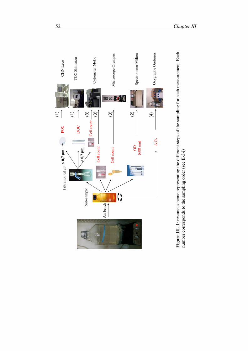
Chapter III 52
Sp
ectr
om
eter
Mil
ton
Fil
trat
ion
GF
/FP
OC
> 0
,7 µ
m
DO
C<
0,7
µm O
D
(600
nm
)
Cyto
met
erM
ofl
o
Ox
ygra
ph
eO
rob
oro
s
Mic
rosc
op
e O
lym
pu
s
Air
ben
ch
CH
N L
eco
TO
C S
him
atzu
Cel
lco
un
t
∆O
2
Su
b-s
amp
le
(1)
(2)
(3)
(1)
(3)
(4)
(3)
Cel
lco
un
t
Cel
lco
un
t
Fig
ure
III
- 1:
resu
me
sch
eme
repre
sen
tin
g t
he
dif
fere
nt
step
s o
f th
e sa
mp
lin
g f
or
each
mea
sure
men
t. E
ach
nu
mb
er c
orr
esp
on
ds
to t
he
sam
pli
ng
ord
er (
see
II-3
-i)
Biodegradation experiments in variable environment 53
3. Sampling method and variable measurements
i. Sampling
To prevent any bacterial and carbon contamination, we did not insert any
material in the culture bottles and handling of samples was done under
laminar flow air bench. Sampling was realised at each point in time by
pouring a certain volume of culture in another pre-combusted borosilicate
bottle that was used for all sub-samples. This sampling technique allows
keeping the culture in the temperate room most of the time. The
measurements were always realised in the same order to avoid any bias due
to the temporal lag between the different measurements. First sub-sampling
was always for carbon measurements (DOC/POC) to prevent any carbon
contamination by the other measurement methods. The sampling order was:
(1) POC/DOC, (2) optical density (OD), (3) cell count by microscopy and
cytometry analyses, and (4) oxygen consumption (Figure III-1). The cultures
were always homogenised before sampling.
ii. DOC
Only DOC concentration in the culture was measured by using the total
carbon analyses that did not give any information about the pyruvate
concentration evolution. At the beginning of the experiment, the other
identified carbon source, except pyruvate, was vitamin-DOC that we have
estimated to comprise only 3 % of DOC when the initial carbon
concentration from pyruvate was 1.6 mM C. When the initial substrate
concentration was 8 mM C, this percentage was thus negligible (0.6 %). The
medium also comprised more than 1 mM C of NaHCO3 that is inorganic and
eliminated by acidification and bubbling before the DOC measurement.
For DOC analyses, a variable amount (10 to 100 cm3) of the sub-sample
was collected in a graduated pre-combusted borosilicate tube and filtered
through a pre-combusted GF/F glass fibre filter (0,7 µm nominal retention
size). DOC was measured by high temperature catalytic oxidation (HTCO)
(Sempéré et al. 2003, Sohrin & Sempéré 2005) using a Shimadzu TOC 5000
Analyzer. Samples were acidified to pH ≈ 1 with 85 % phosphoric acid and
bubbled for 10 minutes with CO2-free air to purge inorganic carbon. Three or
four 100 mm3 replicates of each sample were injected into the column heated
at 680 °C. The effluent passed through a drying unit (magnesium perchlorate
cartridge), a scrubber to eliminate halogen gas and sulfates, a dust-
eliminating membrane filter to remove sea salt and phosphoric acid aerosols,
and finally in non-dispersive infrared (NDIR) cell in which CO2 was
detected. The coefficient of variation of DOC replicates was always smaller
Chapter III 54
than 2 %. Quantification was performed by a four point-calibration curve
with standards (from 0 to 2 mM C for the B1 and P experiments and from 0
to 8.5 mM C for the experiment B2) prepared by diluting potassium
hydrogen phthalate in Milli-Q water.
iii. POC
In this study, POC refers to the bacterial biomass in carbon and was
sampled at the same time as DOC on the filtration column. Indeed, POC is
the part of the sub-sample retained on the GF/F filters. A variable but
sufficient amount of culture volume was filtered in order to have a reliable
POC signal. After the filtration step, each filter was dried in a drying oven,
carefully stored in the dark and then analysed with a carbon analyser (Leco
SC-144). Filters were introduced in a ceramic carrier and the combustion was
carried out at 1350°C in an oxygen flux. The organic carbon is thus
transformed in CO2 and detected by a NDIR cell. Calibration was performed
with reference compound in the same order of magnitude than sample. The
measurement uncertainty was between 3 and 8 % for these carbon
concentrations.
iv. Optical density (OD)
Optical Density (OD) served essentially to check the bacterial growth
during the manipulation. We collected 4 cm3 of the sub-sample to measure
the OD with a spectrometer (Milton for experiments B1 and P and Jenway
6310 for experiment B2). OD was measured at 600 nm, wavelength linked to
particles density. The OD medium value was subtracted to each OD value.
v. O2 consumption
O2 consumption was estimated by measuring the O2 concentration with
the Oroboros-2k oxygraph (OROBOROS, Austria) (Appendix III-B-1). This
oxygraph provides the instrumental basis for temporal high-resolution
respirometry due to a small lag time between two measurements (2 s). As
recommended by the manufacturer the volume of the chambers was set at 2
cm3, and the stirrer speed at 750 rounds per minute.
Each day, a control sample was made with a sterile medium sample to
determine the consumption of the polarographic oxygen sensor (POS). This
value was then subtracted from each O2 consumption value measured the
same day. The POS were calibrated with 0 and 100 % oxygen saturation. The
calibration with 0 % oxygen saturation was done before the start of each new
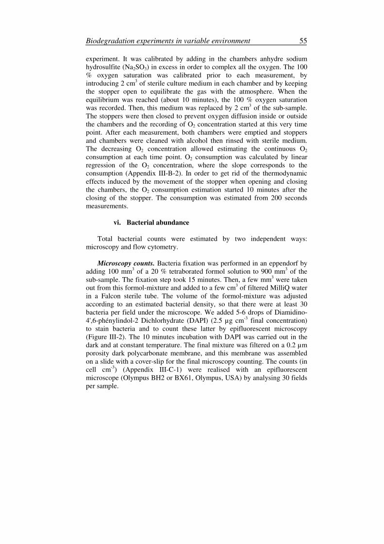
Biodegradation experiments in variable environment 55
experiment. It was calibrated by adding in the chambers anhydre sodium
hydrosulfite (Na2SO3) in excess in order to complex all the oxygen. The 100
% oxygen saturation was calibrated prior to each measurement, by
introducing 2 cm3 of sterile culture medium in each chamber and by keeping
the stopper open to equilibrate the gas with the atmosphere. When the
equilibrium was reached (about 10 minutes), the 100 % oxygen saturation
was recorded. Then, this medium was replaced by 2 cm3 of the sub-sample.
The stoppers were then closed to prevent oxygen diffusion inside or outside
the chambers and the recording of O2 concentration started at this very time
point. After each measurement, both chambers were emptied and stoppers
and chambers were cleaned with alcohol then rinsed with sterile medium.
The decreasing O2 concentration allowed estimating the continuous O2
consumption at each time point. O2 consumption was calculated by linear
regression of the O2 concentration, where the slope corresponds to the
consumption (Appendix III-B-2). In order to get rid of the thermodynamic
effects induced by the movement of the stopper when opening and closing
the chambers, the O2 consumption estimation started 10 minutes after the
closing of the stopper. The consumption was estimated from 200 seconds
measurements.
vi. Bacterial abundance
Total bacterial counts were estimated by two independent ways:
microscopy and flow cytometry.
Microscopy counts. Bacteria fixation was performed in an eppendorf by
adding 100 mm3 of a 20 % tetraborated formol solution to 900 mm
3 of the
sub-sample. The fixation step took 15 minutes. Then, a few mm3 were taken
out from this formol-mixture and added to a few cm3 of filtered MilliQ water
in a Falcon sterile tube. The volume of the formol-mixture was adjusted
according to an estimated bacterial density, so that there were at least 30
bacteria per field under the microscope. We added 5-6 drops of Diamidino-
4',6-phénylindol-2 Dichlorhydrate (DAPI) (2.5 µg cm-3
final concentration)
to stain bacteria and to count these latter by epifluorescent microscopy
(Figure III-2). The 10 minutes incubation with DAPI was carried out in the
dark and at constant temperature. The final mixture was filtered on a 0.2 µm
porosity dark polycarbonate membrane, and this membrane was assembled
on a slide with a cover-slip for the final microscopy counting. The counts (in
cell cm-3
) (Appendix III-C-1) were realised with an epifluorescent
microscope (Olympus BH2 or BX61, Olympus, USA) by analysing 30 fields
per sample.
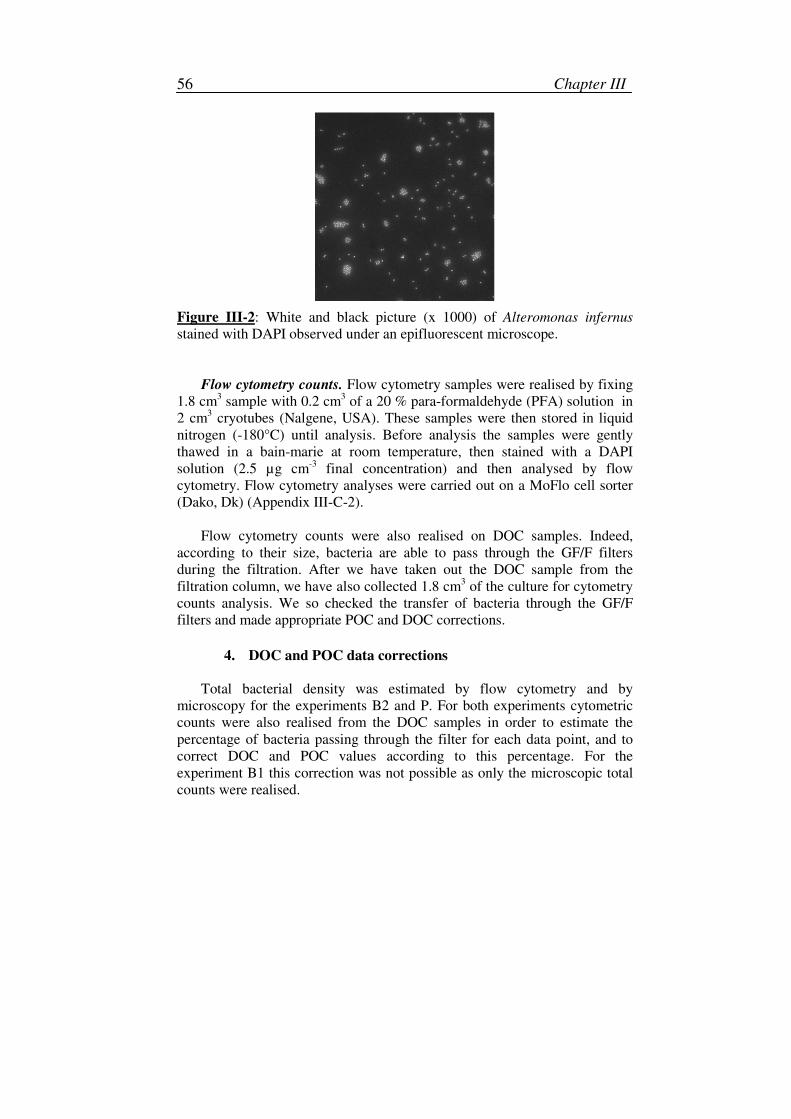
Chapter III 56
Figure III-2: White and black picture (x 1000) of Alteromonas infernus
stained with DAPI observed under an epifluorescent microscope.
Flow cytometry counts. Flow cytometry samples were realised by fixing
1.8 cm3 sample with 0.2 cm
3 of a 20 % para-formaldehyde (PFA) solution in
2 cm3 cryotubes (Nalgene, USA). These samples were then stored in liquid
nitrogen (-180°C) until analysis. Before analysis the samples were gently
thawed in a bain-marie at room temperature, then stained with a DAPI
solution (2.5 µg cm-3
final concentration) and then analysed by flow
cytometry. Flow cytometry analyses were carried out on a MoFlo cell sorter
(Dako, Dk) (Appendix III-C-2).
Flow cytometry counts were also realised on DOC samples. Indeed,
according to their size, bacteria are able to pass through the GF/F filters
during the filtration. After we have taken out the DOC sample from the
filtration column, we have also collected 1.8 cm3 of the culture for cytometry
counts analysis. We so checked the transfer of bacteria through the GF/F
filters and made appropriate POC and DOC corrections.
4. DOC and POC data corrections
Total bacterial density was estimated by flow cytometry and by
microscopy for the experiments B2 and P. For both experiments cytometric
counts were also realised from the DOC samples in order to estimate the
percentage of bacteria passing through the filter for each data point, and to
correct DOC and POC values according to this percentage. For the
experiment B1 this correction was not possible as only the microscopic total
counts were realised.
Biodegradation experiments in variable environment 57
i. Experiment B2
We noticed that bacterial dynamics are qualitatively identical for both
techniques of bacterial density estimation, although the cytometry leads to an
overestimation of the total bacterial counts (Figure III-3). This phenomenon
has already been mentioned in the literature (Monfort & Baleux 1992).
Assuming the flow cytometry as the reference technique, this difference is
highly variable during the time course of the experiment, ranging from - 5 to
54 %. This difference is higher during the exponential growth phase (34 to 54
% of difference) than during other growth phases (- 5 to 30 %).
20 40 60 800
1
2
3
4
5
6
7x 10
8D
ensi
ty (
bact
cm
-3)
time (h)
microscopycytometry
Figure III- 3: Comparison of bacterial density estimated with the MoFlo
cytometer (o) and the epifluorescent microscope (+) after DAPI staining for
the B2 experiment.
Density of bacteria passing through the filter during DOC/POC
separation was estimated by MoFlo flow cytometer. For the B2 experiment,
percentage of bacteria in the DOC samples was estimated to range from 0 to
14 %. Higher values were obtained during the exponential growth phase,
whereas this percentage was near 0 % during the lag and the stationary
phases. This suggests that bacteria are larger during non dividing period, and
that the cell division leads to shrinking of bacteria, which subsequently
reached the limit size of the filter retention size. We have then multiplied this
percentage by the POC value at each point in time to estimate the bacterial
biomass that has been considered as DOC instead of POC. This biomass was
thus subtracted from the DOC values and added to the POC values for each
sampling point.
Chapter III 58
ii. Experiment P
Unfortunately, unfiltered samples and some filtered samples for the pulse
experiment were not measured for bacterial density with cytometry due to
technical problems. Thus, the percentage of bacteria passing through the
filters was estimated by comparing the bacterial density analysed by
epifluorescent microscopy in the full sample to the bacterial density analysed
by cytometry after the filtration. In the B2 experiment the density values
were always higher (except for one data point) when they were analysed by
cytometry. As this phenomenon was already mentioned for other studies
(Monfort & Baleux 1992), we can assume that the same result occurs for the
P experiment. Thus, by calculating the percentage of bacteria going through
the filters with a reference to the microscopic total counts instead of to the
cytometric total counts, we introduce a bias, overestimating this percentage.
Moreover, except two values of 10.8 and 12.8 %, the percentage of bacteria
in the DOC samples was always inferior to 4.5 %. Due to this low
percentage, to its overestimation and to the lack of some data, we have
decided to not correct the DOC and POC data for the pulse experiment.
5. BGE estimation
For BGE estimation, we focused on the batch experiment B2 and the
pulse experiment P. The only difference between both experiments is the way
of supplying substrate to the batch cultures. Indeed, all the substrate was
available at the beginning of the batch experiment, therefore the culture was
not exposed to any perturbation during the time course of the experiment. By
contrast, in the pulse experiment, substrate was periodically added in the
batch culture. Note that the total substrate quantity added was the same in
both experiments. We are specifically interested in the bacterial efficiency to
assimilate the C-substrate and in their growth pattern. Here, BGE was
calculated by using experimental data points and modelling methods.
i. Experimental BGE estimation
The experimental BGE estimation has been widely used in
microbiological studies, especially using in situ samples, to compare the
ability of bacteria to use DOC for their growth (del Giorgio & Cole 1998).
BGE can be experimentally calculated with the following formula: BGE =
BP/BCD and BCD = BP + BR (Carlson & Ducklow 1996, del Giorgio &
Cole 1998, Rivkin & Legendre 2001, Sempéré et al. 2003, Cherrier & Bauer
2004) where BCD is the bacterial carbon demand, BP the bacterial
production and BR the bacterial respiration. In this study, BP was not
Biodegradation experiments in variable environment 59
measured but it was estimated by the difference between the maximum and
initial POC values. BCD was estimated as the difference between the initial
(experiment B2) or the total substrate quantity put in the culture (experiment
P) and the remaining DOC at the end of the experiment.
ii. BGE estimation from models
BGE has also been estimated by using three models with different levels
of detail. The first model originates from the dynamic energy budget (DEB)
theory (Kooijman 2000) and has been especially constructed for the pulse
experiment due to the presence of the starvation periods. This model
comprises a reserve compartment as well as two maintenance processes:
maintenance is paid from mobilized reserve if the flux is large enough, but
otherwise structure is used to pay the remaining part of the maintenance
costs, which causes shrinking of the cell (Tolla et al. 2007, Eichinger et al.
submitted – chapter IV) (equations III-3). Consequently, growth is not
realised directly from assimilation but is buffered by the reserve
compartment. When maintenance is realised from the structural biomass,
bacteria release maintenance products in the culture, which correspond to R-
DOC. The BGE of this latter model corresponds to the parameter Y, ratio of
the two primary parameters EL
y and EV
y (Table III-1).
The second model is the Marr-Pirt model (Marr et al. 1963, Pirt 1965),
which assumes a direct transfer from assimilation to growth, but which also
includes a maintenance term. However, maintenance is only realised from the
structural biomass as this model does not comprise any reserve compartment
(equations III-2). As in the DEB model, R-DOC is produced from the
maintenance of the biomass. BGE corresponds to the parameter VL
Y of this
model (Table III-1).
The third model is the Monod model (Monod 1942), which includes
neither reserve nor maintenance. It only assumes that the substrate is directly
and instantaneously transformed in biomass with a constant efficiency, the
BGE (Table III-1 and equations III-1). Note that here we also report that
bacteria were able to produce refractory materials in our systems. However,
this model does not allow any product formation. Consequently, in order to
compare parameters governing assimilation and growth on L-DOC between
the three models, DOC data were modified to deal only with the labile
fraction of DOC. DOC values were set to zero during stationary phase. The
way to modify data to focus on L-DOC was different for each experiment.
For the B2 experiment, R-DOC concentration seems constant. L-DOC values
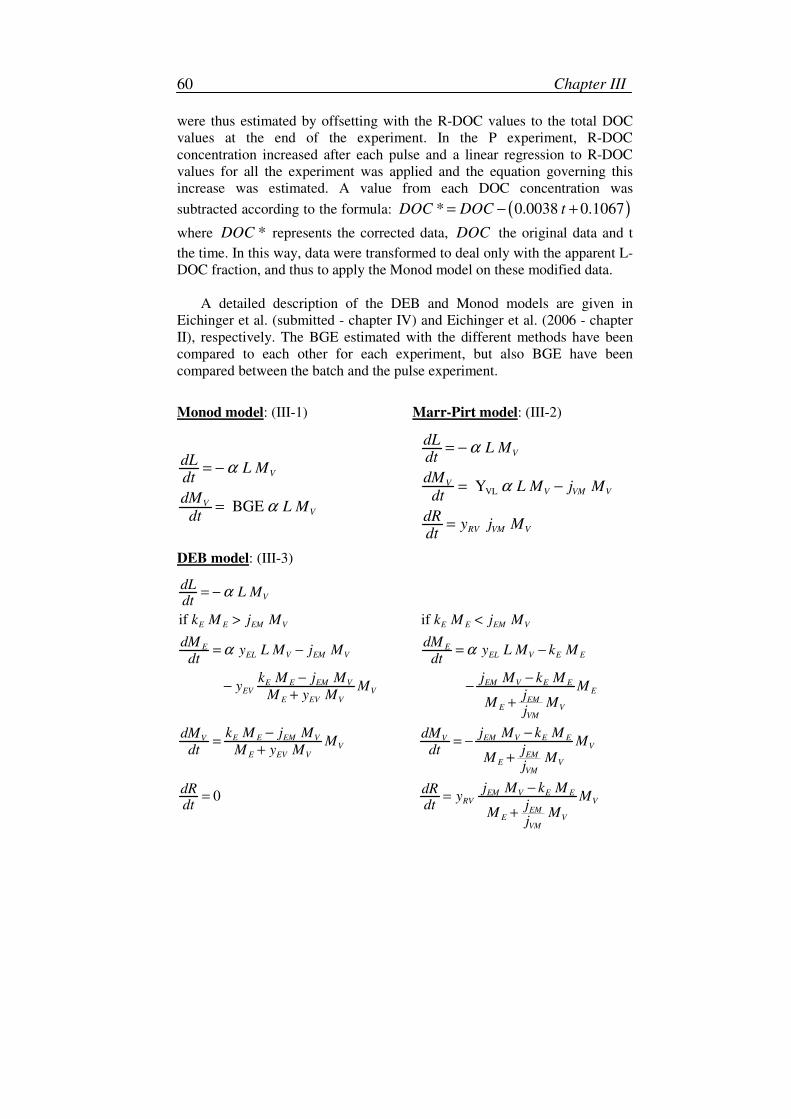
Chapter III 60
were thus estimated by offsetting with the R-DOC values to the total DOC
values at the end of the experiment. In the P experiment, R-DOC
concentration increased after each pulse and a linear regression to R-DOC
values for all the experiment was applied and the equation governing this
increase was estimated. A value from each DOC concentration was
subtracted according to the formula: ( )* 0.0038 0.1067DOC DOC t= − +
where *DOC represents the corrected data, DOC the original data and t
the time. In this way, data were transformed to deal only with the apparent L-
DOC fraction, and thus to apply the Monod model on these modified data.
A detailed description of the DEB and Monod models are given in
Eichinger et al. (submitted - chapter IV) and Eichinger et al. (2006 - chapter
II), respectively. The BGE estimated with the different methods have been
compared to each other for each experiment, but also BGE have been
compared between the batch and the pulse experiment.
Monod model: (III-1) Marr-Pirt model: (III-2)
BGE
V
VV
dLL M
dt
dML M
dt
α
α
= −
=
VL Y
V
VV VM V
RV VM V
dLL M
dt
dML M j M
dt
dRy j M
dt
α
α
= −
= −
=
DEB model: (III-3)
if if
0
V
E E EM V E E EM V
E EEL V EM V EL V E E
E E EM V EM V E EEV V E
E EV V EME V
VM
E E EM V EM V E EV VV V
E EV V EME V
VM
EM V ERV
dLL M
dt
k M j M k M j M
dM dMy L M j M y L M k M
dt dt
k M j M j M k My M M
M y M jM M
j
k M j M j M k MdM dMM M
dt M y M dt jM M
j
j M kdR dRy
dt dt
α
α α
= −
> <
= − = −
− −− −
++
− −= = −
++
−= = E
VEM
E VVM
MM
jM M
j+
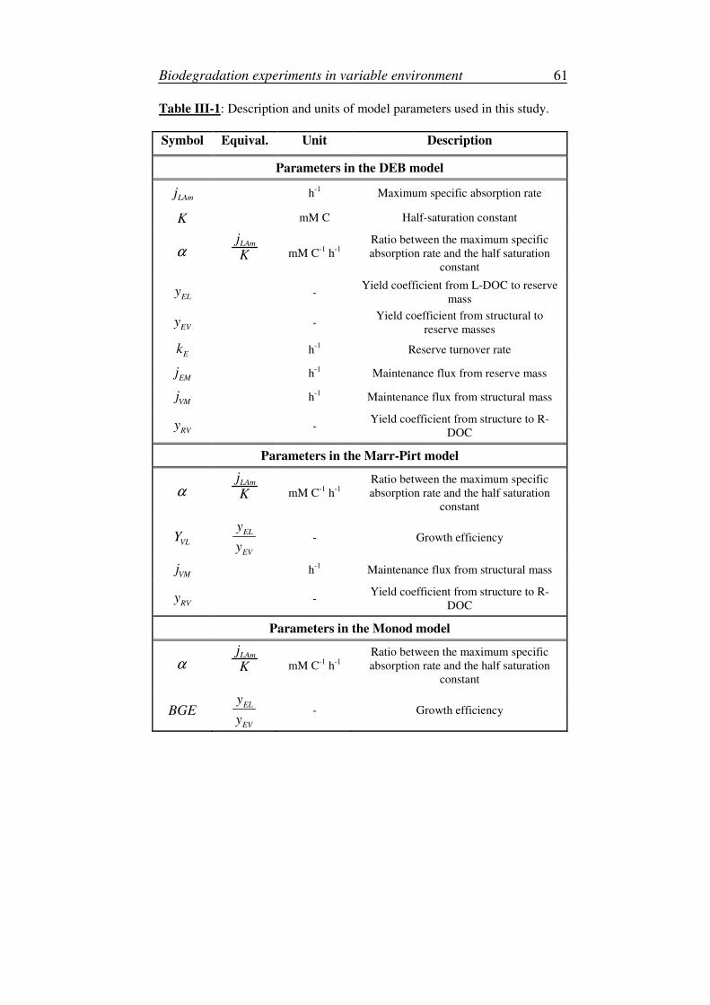
Biodegradation experiments in variable environment 61
Table III-1: Description and units of model parameters used in this study.
Symbol Equival. Unit Description
Parameters in the DEB model
LAmj
h-1
Maximum specific absorption rate
K mM C Half-saturation constant
α LAmj
K
mM C-1
h-1
Ratio between the maximum specific
absorption rate and the half saturation
constant
ELy
-
Yield coefficient from L-DOC to reserve
mass
EVy
-
Yield coefficient from structural to
reserve masses
Ek h
-1 Reserve turnover rate
EMj h
-1 Maintenance flux from reserve mass
VMj h
-1 Maintenance flux from structural mass
RVy
-
Yield coefficient from structure to R-
DOC
Parameters in the Marr-Pirt model
α LAmj
K
mM C-1
h-1
Ratio between the maximum specific
absorption rate and the half saturation
constant
VLY
EL
EV
y
y - Growth efficiency
VMj h
-1 Maintenance flux from structural mass
RVy
-
Yield coefficient from structure to R-
DOC
Parameters in the Monod model
α LAmj
K
mM C-1
h-1
Ratio between the maximum specific
absorption rate and the half saturation
constant
BGE EL
EV
y
y - Growth efficiency
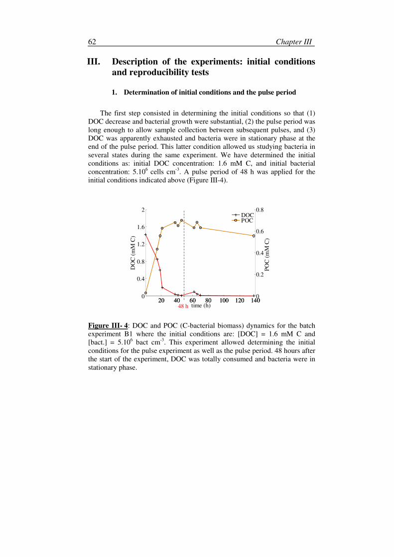
Chapter III 62
III. Description of the experiments: initial conditions
and reproducibility tests
1. Determination of initial conditions and the pulse period
The first step consisted in determining the initial conditions so that (1)
DOC decrease and bacterial growth were substantial, (2) the pulse period was
long enough to allow sample collection between subsequent pulses, and (3)
DOC was apparently exhausted and bacteria were in stationary phase at the
end of the pulse period. This latter condition allowed us studying bacteria in
several states during the same experiment. We have determined the initial
conditions as: initial DOC concentration: 1.6 mM C, and initial bacterial
concentration: 5.106 cells cm
-3. A pulse period of 48 h was applied for the
initial conditions indicated above (Figure III-4).
20 40 60 80 100 120 1400
0.4
0.8
1.2
1.6
2
DO
C (
mM
C)
20 40 60 80 100 120 1400
0.2
0.4
0.6
0.8
PO
C (
mM
C)
time (h)
DOCPOC
48 h
Figure III- 4: DOC and POC (C-bacterial biomass) dynamics for the batch
experiment B1 where the initial conditions are: [DOC] = 1.6 mM C and
[bact.] = 5.106 bact cm
-3. This experiment allowed determining the initial
conditions for the pulse experiment as well as the pulse period. 48 hours after
the start of the experiment, DOC was totally consumed and bacteria were in
stationary phase.
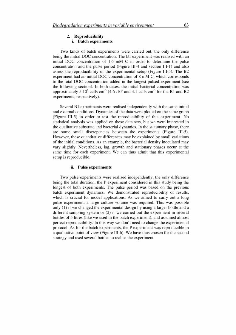
Biodegradation experiments in variable environment 63
2. Reproducibility
i. Batch experiments
Two kinds of batch experiments were carried out, the only difference
being the initial DOC concentration. The B1 experiment was realised with an
initial DOC concentration of 1.6 mM C in order to determine the pulse
concentration and the pulse period (Figure III-4 and section III-1) and also
assess the reproducibility of the experimental setup (Figure III-5). The B2
experiment had an initial DOC concentration of 8 mM C, which corresponds
to the total DOC concentration added in the longest pulsed experiment (see
the following section). In both cases, the initial bacterial concentration was
approximately 5.106 cells cm
-3 (4.6 .10
6 and 4.1 cells cm
-3 for the B1 and B2
experiments, respectively).
Several B1 experiments were realised independently with the same initial
and external conditions. Dynamics of the data were plotted on the same graph
(Figure III-5) in order to test the reproducibility of this experiment. No
statistical analysis was applied on these data sets, but we were interested in
the qualitative substrate and bacterial dynamics. In the stationary phase, there
are some small discrepancies between the experiments (Figure III-5).
However, these quantitative differences may be explained by small variations
of the initial conditions. As an example, the bacterial density inoculated may
vary slightly. Nevertheless, lag, growth and stationary phases occur at the
same time for each experiment. We can thus admit that this experimental
setup is reproducible.
ii. Pulse experiments
Two pulse experiments were realised independently, the only difference
being the total duration, the P experiment considered in this study being the
longest of both experiments. The pulse period was based on the previous
batch experiment dynamics. We demonstrated reproducibility of results,
which is crucial for model applications. As we aimed to carry out a long
pulse experiment, a large culture volume was required. This was possible
only (1) if we changed the experimental design by using a larger bottle and a
different sampling system or (2) if we carried out the experiment in several
bottles of 5 litres (like we used in the batch experiment), and assumed almost
perfect reproducibility. In this way we don’t need to change the experimental
protocol. As for the batch experiments, the P experiment was reproducible in
a qualitative point of view (Figure III-6). We have thus chosen for the second
strategy and used several bottles to realise the experiment.
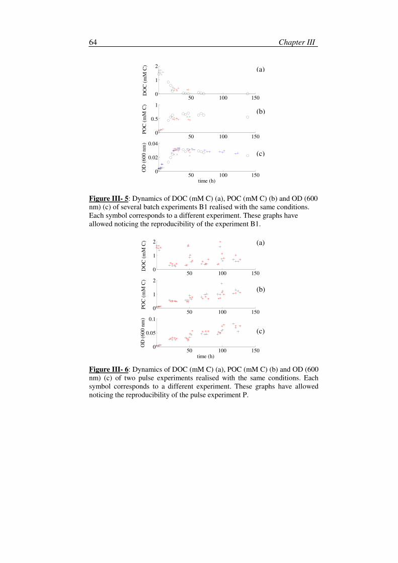
Chapter III 64
50 100 1500
1
2
DO
C (
mM
C)
50 100 1500
0.5
1
PO
C (
mM
C)
50 100 1500
0.02
0.04O
D (
60
0 n
m)
time (h)
Figure III- 5: Dynamics of DOC (mM C) (a), POC (mM C) (b) and OD (600
nm) (c) of several batch experiments B1 realised with the same conditions.
Each symbol corresponds to a different experiment. These graphs have
allowed noticing the reproducibility of the experiment B1.
50 100 1500
1
2
DO
C (
mM
C)
50 100 1500
1
2
PO
C (
mM
C)
50 100 1500
0.05
0.1
OD
(600 n
m)
time (h)
Figure III- 6: Dynamics of DOC (mM C) (a), POC (mM C) (b) and OD (600
nm) (c) of two pulse experiments realised with the same conditions. Each
symbol corresponds to a different experiment. These graphs have allowed
noticing the reproducibility of the pulse experiment P.
(b)
(a)
(c)
(a)
(b)
(c)
Biodegradation experiments in variable environment 65
IV. Identification of key processes
1. Autocorrelation of bacterial measurements
For each experiment, we noticed that the dynamics of bacterial variables,
i.e. POC, OD and the abundance, were very close, especially for the batch
experiments (Figures III-7 and 8 a-b). To test the correlation between these
measurements, we applied linear regressions on OD and abundance data
against POC data (Figures III-7 to III-9 c-d). The correlation coefficients
were always higher than 0.8, except one value (0.38) for the P experiment
(Figure III-9-c) and always better for the batch than for the pulse
experiments. Bacterial density showed high variations for this experiment.
The correlation coefficient for OD against POC is always larger than 0.9,
except for the experiment P as we had some technical problems with the
spectrometer. We missed some data points due to this problem and needed to
change the light source, which may explain some variations in the data set.
Correlation coefficients estimated from abundance data are always inferior,
which may be explained by the fact that the correlation seems less accurate
during the stationary phase (Figures III-7 to III-9 a). However, as critical
value p < 0.005 for all tests, these results exhibit a significant autocorrelation
between the several variables used to measure bacterial growth in this study.
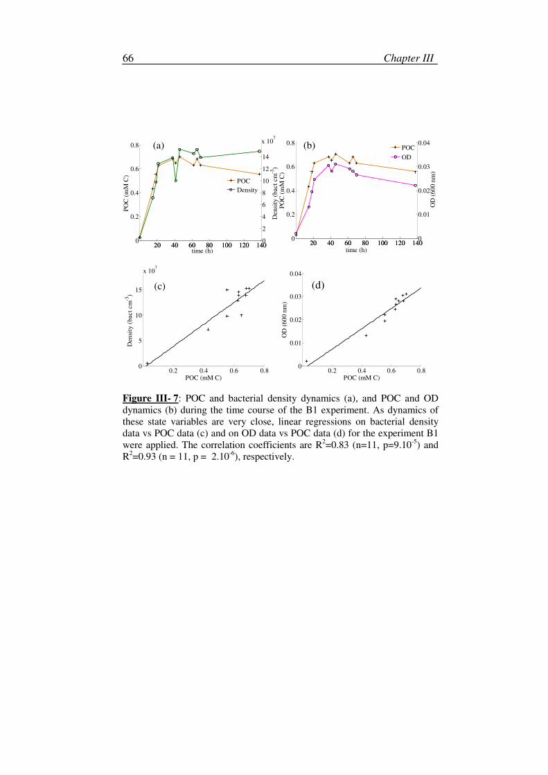
Chapter III 66
20 40 60 80 100 120 1400
0.2
0.4
0.6
0.8
PO
C (
mM
C)
20 40 60 80 100 120 1400
2
4
6
8
10
12
14
x 107
Densi
ty (
bact
cm
-3)
time (h)
POC
Density
20 40 60 80 100 120 1400
0.2
0.4
0.6
0.8
PO
C (
mM
C)
20 40 60 80 100 120 1400
0.01
0.02
0.03
0.04
OD
(60
0 n
m)
time (h)
POC
OD
0.2 0.4 0.6 0.80
5
10
15
x 107
Den
sity
(bact
cm
-3)
POC (mM C)0.2 0.4 0.6 0.8
0
0.01
0.02
0.03
0.04
OD
(60
0 n
m)
POC (mM C)
Figure III- 7: POC and bacterial density dynamics (a), and POC and OD
dynamics (b) during the time course of the B1 experiment. As dynamics of
these state variables are very close, linear regressions on bacterial density
data vs POC data (c) and on OD data vs POC data (d) for the experiment B1
were applied. The correlation coefficients are R2=0.83 (n=11, p=9.10
-5) and
R2=0.93 (n = 11, p = 2.10
-6), respectively.
(c)
(a) (b)
(d)
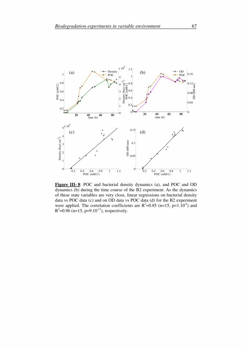
Biodegradation experiments in variable environment 67
20 40 60 80
0.2
0.4
0.6
0.8
1
PO
C (
mM
C)
20 40 60 800
1
2
3
4
5
x 108
Den
sity
(bact
cm
-3)
time (h)
POC
Density
20 40 60 800
0.2
0.4
0.6
0.8
1
1.2
PO
C (
mM
C)
20 40 60 800
0.04
0.08
0.12
0.16
OD
(600
nm
)
time (h)
POC
OD
0.2 0.4 0.6 0.8 1 1.20
1
2
3
4
5x 10
8
Den
sity
(bact
cm
-3)
POC (mM C)0.2 0.4 0.6 0.8 1 1.2
0
0.05
0.1
0.15O
D (
60
0 n
m)
POC (mM C) Figure III- 8: POC and bacterial density dynamics (a), and POC and OD
dynamics (b) during the time course of the B2 experiment. As the dynamics
of these state variables are very close, linear regressions on bacterial density
data vs POC data (c) and on OD data vs POC data (d) for the B2 experiment
were applied. The correlation coefficients are R2=0.85 (n=15, p=1.10
-6) and
R2=0.96 (n=15, p=9.10
-11), respectively.
(b) (a)
(c) (d)
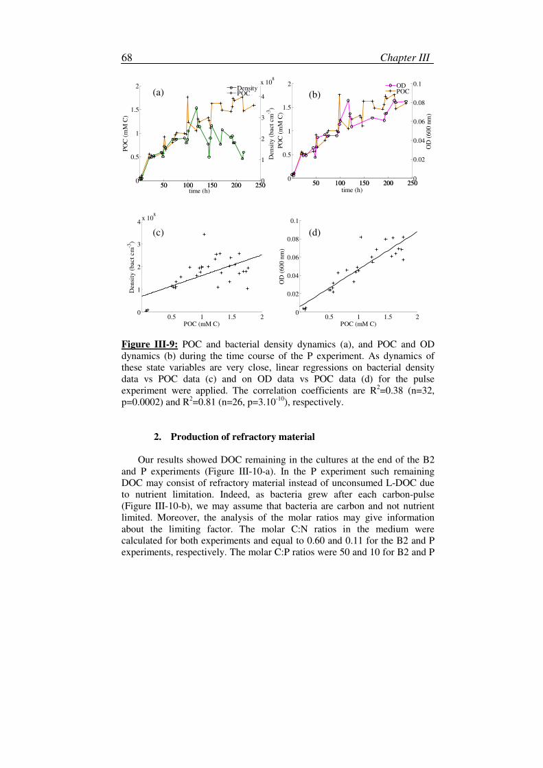
Chapter III 68
50 100 150 200 2500
0.5
1
1.5
2
PO
C (
mM
C)
50 100 150 200 2500
1
2
3
4
x 108
Den
sity
(bact
cm
-3)
time (h)
POCDensity
50 100 150 200 2500
0.5
1
1.5
2
PO
C (
mM
C)
50 100 150 200 2500
0.02
0.04
0.06
0.08
0.1
OD
(6
00 n
m)
time (h)
POCOD
0.5 1 1.5 20
1
2
3
4x 10
8
Den
sity
(bact
cm
-3)
POC (mM C)0.5 1 1.5 2
0
0.02
0.04
0.06
0.08
0.1
OD
(60
0 n
m)
POC (mM C)
Figure III-9: POC and bacterial density dynamics (a), and POC and OD
dynamics (b) during the time course of the P experiment. As dynamics of
these state variables are very close, linear regressions on bacterial density
data vs POC data (c) and on OD data vs POC data (d) for the pulse
experiment were applied. The correlation coefficients are R2=0.38 (n=32,
p=0.0002) and R2=0.81 (n=26, p=3.10
-10), respectively.
2. Production of refractory material
Our results showed DOC remaining in the cultures at the end of the B2
and P experiments (Figure III-10-a). In the P experiment such remaining
DOC may consist of refractory material instead of unconsumed L-DOC due
to nutrient limitation. Indeed, as bacteria grew after each carbon-pulse
(Figure III-10-b), we may assume that bacteria are carbon and not nutrient
limited. Moreover, the analysis of the molar ratios may give information
about the limiting factor. The molar C:N ratios in the medium were
calculated for both experiments and equal to 0.60 and 0.11 for the B2 and P
experiments, respectively. The molar C:P ratios were 50 and 10 for B2 and P
(b) (a)
(d) (c)
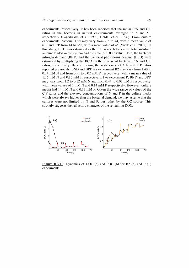
Biodegradation experiments in variable environment 69
experiments, respectively. It has been reported that the molar C:N and C:P
ratios in the bacteria in natural environments averaged to 5 and 50,
respectively (Fagerbakke et al. 1996, Heldal et al. 1996). From culture
experiments, bacterial C:N may vary from 2.3 to 44, with a mean value of
6.1, and C:P from 14 to 358, with a mean value of 45 (Vrede et al. 2002). In
this study, BCD was estimated as the difference between the total substrate
amount loaded in the system and the smallest DOC value. Here, the bacterial
nitrogen demand (BND) and the bacterial phosphorus demand (BPD) were
estimated by multiplying the BCD by the inverse of bacterial C:N and C:P
ratios, respectively. By considering the wide range of C:N and C:P ratios
reported previously, BND and BPD for experiment B2 may vary from 1.40 to
0.14 mM N and from 0.51 to 0.02 mM P, respectively, with a mean value of
1.16 mM N and 0.16 mM P, respectively. For experiment P, BND and BPD
may vary from 1.2 to 0.12 mM N and from 0.44 to 0.02 mM P respectively,
with mean values of 1 mM N and 0.14 mM P respectively. However, culture
media had 14 mM N and 0.17 mM P. Given the wide range of values of the
C:P ratios and the elevated concentrations of N and P in the culture media
which were always higher than the bacterial demand, we may assume that the
cultures were not limited by N and P, but rather by the OC source. This
strongly suggests the refractory character of the remaining DOC.
50 100 150 200 2500
2
4
6
8
10
DO
C (
mM
C)
time (h)
batch
pulse
50 100 150 200 2500
0.5
1
1.5
2
PO
C (
mM
C)
time (h)
batchpulse
Figure III- 10: Dynamics of DOC (a) and POC (b) for B2 (o) and P (+)
experiments.
(a) (b)
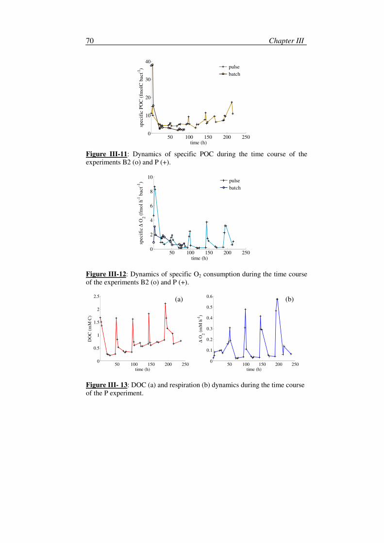
Chapter III 70
50 100 150 200 2500
10
20
30
40
spec
ific
PO
C (
fmo
lC b
act-1
)time (h)
batch
pulse
Figure III-11: Dynamics of specific POC during the time course of the
experiments B2 (o) and P (+).
50 100 150 200 2500
2
4
6
8
10
specif
ic ∆
O2 (
fmo
l h-1
bact-1
)
time (h)
batch
pulse
Figure III-12: Dynamics of specific O2 consumption during the time course
of the experiments B2 (o) and P (+).
50 100 150 200 2500
0.5
1
1.5
2
2.5
DO
C (
mM
C)
time (h)50 100 150 200 250
0
0.1
0.2
0.3
0.4
0.5
0.6
∆ O
2 (
mM
h-1
)
time (h)
Figure III- 13: DOC (a) and respiration (b) dynamics during the time course
of the P experiment.
(a) (b)
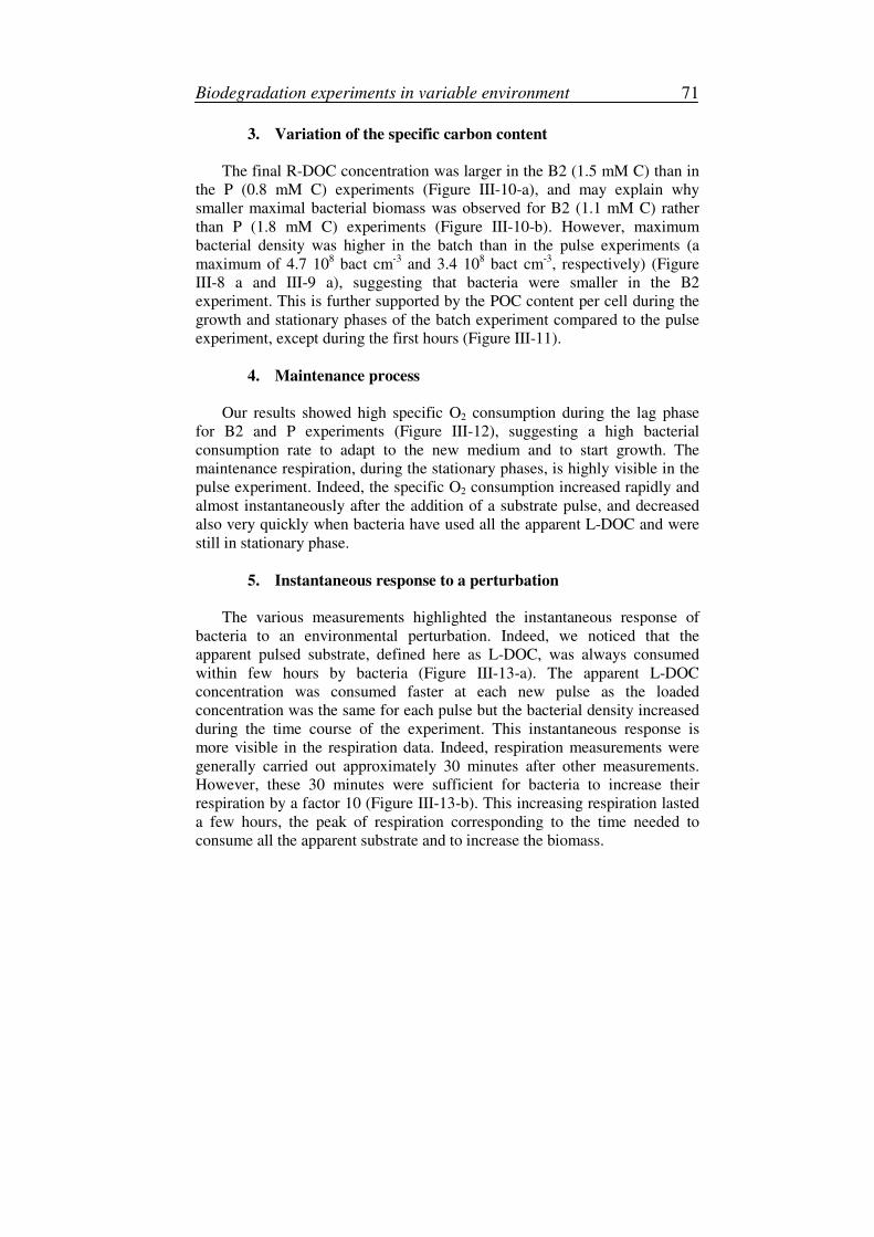
Biodegradation experiments in variable environment 71
3. Variation of the specific carbon content
The final R-DOC concentration was larger in the B2 (1.5 mM C) than in
the P (0.8 mM C) experiments (Figure III-10-a), and may explain why
smaller maximal bacterial biomass was observed for B2 (1.1 mM C) rather
than P (1.8 mM C) experiments (Figure III-10-b). However, maximum
bacterial density was higher in the batch than in the pulse experiments (a
maximum of 4.7 108 bact cm
-3 and 3.4 10
8 bact cm
-3, respectively) (Figure
III-8 a and III-9 a), suggesting that bacteria were smaller in the B2
experiment. This is further supported by the POC content per cell during the
growth and stationary phases of the batch experiment compared to the pulse
experiment, except during the first hours (Figure III-11).
4. Maintenance process
Our results showed high specific O2 consumption during the lag phase
for B2 and P experiments (Figure III-12), suggesting a high bacterial
consumption rate to adapt to the new medium and to start growth. The
maintenance respiration, during the stationary phases, is highly visible in the
pulse experiment. Indeed, the specific O2 consumption increased rapidly and
almost instantaneously after the addition of a substrate pulse, and decreased
also very quickly when bacteria have used all the apparent L-DOC and were
still in stationary phase.
5. Instantaneous response to a perturbation
The various measurements highlighted the instantaneous response of
bacteria to an environmental perturbation. Indeed, we noticed that the
apparent pulsed substrate, defined here as L-DOC, was always consumed
within few hours by bacteria (Figure III-13-a). The apparent L-DOC
concentration was consumed faster at each new pulse as the loaded
concentration was the same for each pulse but the bacterial density increased
during the time course of the experiment. This instantaneous response is
more visible in the respiration data. Indeed, respiration measurements were
generally carried out approximately 30 minutes after other measurements.
However, these 30 minutes were sufficient for bacteria to increase their
respiration by a factor 10 (Figure III-13-b). This increasing respiration lasted
a few hours, the peak of respiration corresponding to the time needed to
consume all the apparent substrate and to increase the biomass.
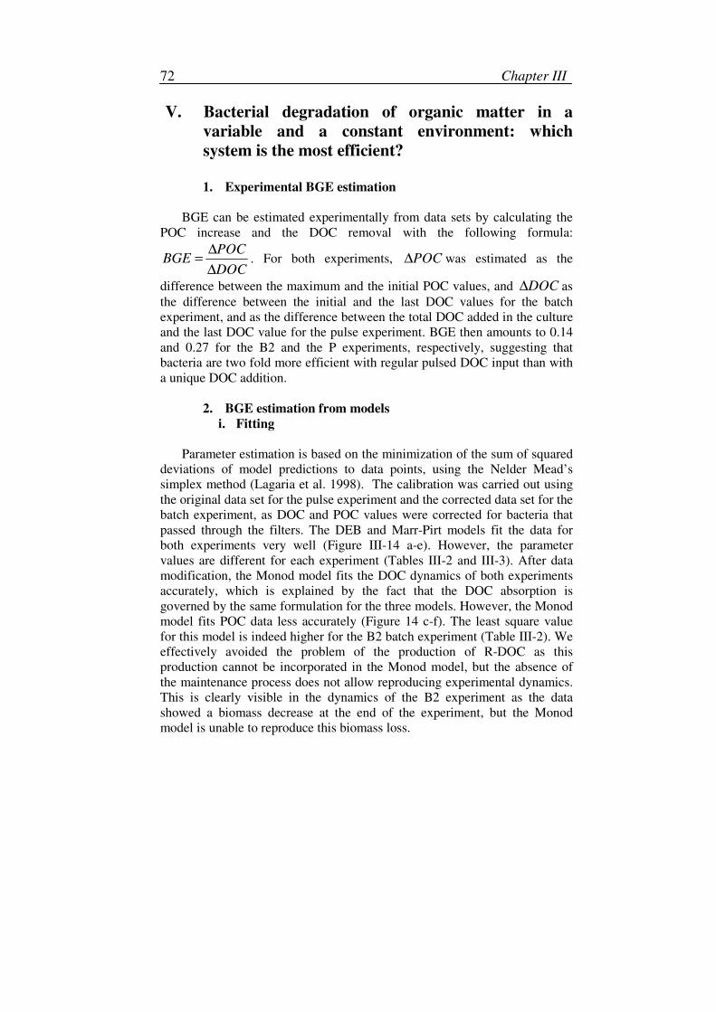
Chapter III 72
V. Bacterial degradation of organic matter in a
variable and a constant environment: which
system is the most efficient?
1. Experimental BGE estimation
BGE can be estimated experimentally from data sets by calculating the
POC increase and the DOC removal with the following formula:
POCBGE
DOC
∆=
∆
. For both experiments, POC∆ was estimated as the
difference between the maximum and the initial POC values, and DOC∆ as
the difference between the initial and the last DOC values for the batch
experiment, and as the difference between the total DOC added in the culture
and the last DOC value for the pulse experiment. BGE then amounts to 0.14
and 0.27 for the B2 and the P experiments, respectively, suggesting that
bacteria are two fold more efficient with regular pulsed DOC input than with
a unique DOC addition.
2. BGE estimation from models
i. Fitting
Parameter estimation is based on the minimization of the sum of squared
deviations of model predictions to data points, using the Nelder Mead’s
simplex method (Lagaria et al. 1998). The calibration was carried out using
the original data set for the pulse experiment and the corrected data set for the
batch experiment, as DOC and POC values were corrected for bacteria that
passed through the filters. The DEB and Marr-Pirt models fit the data for
both experiments very well (Figure III-14 a-e). However, the parameter
values are different for each experiment (Tables III-2 and III-3). After data
modification, the Monod model fits the DOC dynamics of both experiments
accurately, which is explained by the fact that the DOC absorption is
governed by the same formulation for the three models. However, the Monod
model fits POC data less accurately (Figure 14 c-f). The least square value
for this model is indeed higher for the B2 batch experiment (Table III-2). We
effectively avoided the problem of the production of R-DOC as this
production cannot be incorporated in the Monod model, but the absence of
the maintenance process does not allow reproducing experimental dynamics.
This is clearly visible in the dynamics of the B2 experiment as the data
showed a biomass decrease at the end of the experiment, but the Monod
model is unable to reproduce this biomass loss.
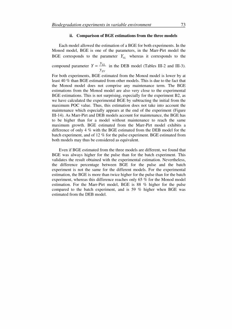
Biodegradation experiments in variable environment 73
ii. Comparison of BGE estimations from the three models
Each model allowed the estimation of a BGE for both experiments. In the
Monod model, BGE is one of the parameters, in the Marr-Pirt model the
BGE corresponds to the parameter VL
Y whereas it corresponds to the
compound parameter EL
EV
yY
y= in the DEB model (Tables III-2 and III-3).
For both experiments, BGE estimated from the Monod model is lower by at
least 40 % than BGE estimated from other models. This is due to the fact that
the Monod model does not comprise any maintenance term. The BGE
estimations from the Monod model are also very close to the experimental
BGE estimations. This is not surprising, especially for the experiment B2, as
we have calculated the experimental BGE by subtracting the initial from the
maximum POC value. Thus, this estimation does not take into account the
maintenance which especially appears at the end of the experiment (Figure
III-14). As Marr-Pirt and DEB models account for maintenance, the BGE has
to be higher than for a model without maintenance to reach the same
maximum growth. BGE estimated from the Marr-Pirt model exhibits a
difference of only 4 % with the BGE estimated from the DEB model for the
batch experiment, and of 12 % for the pulse experiment. BGE estimated from
both models may thus be considered as equivalent.
Even if BGE estimated from the three models are different, we found that
BGE was always higher for the pulse than for the batch experiment. This
validates the result obtained with the experimental estimation. Nevertheless,
the difference percentage between BGE for the pulse and the batch
experiment is not the same for the different models. For the experimental
estimation, the BGE is more than twice higher for the pulse than for the batch
experiment, whereas this difference reaches only 65 % for the Monod model
estimation. For the Marr-Pirt model, BGE is 88 % higher for the pulse
compared to the batch experiment, and is 59 % higher when BGE was
estimated from the DEB model.
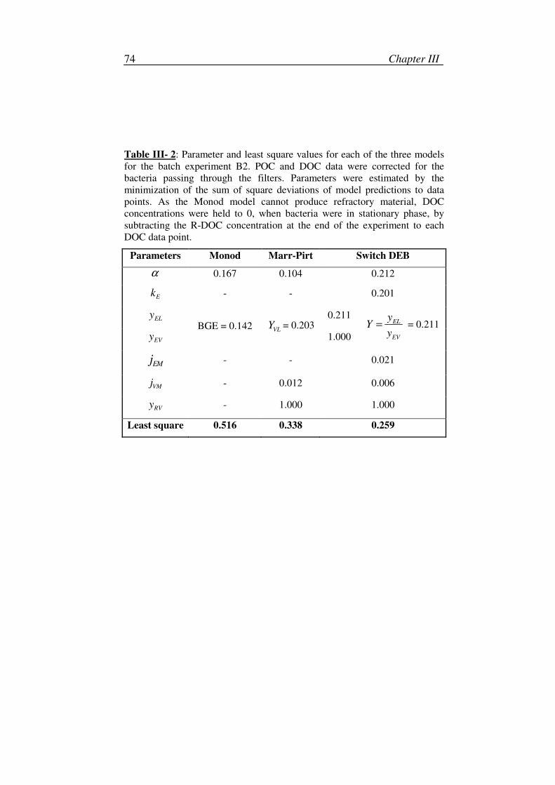
Chapter III 74
Table III- 2: Parameter and least square values for each of the three models
for the batch experiment B2. POC and DOC data were corrected for the
bacteria passing through the filters. Parameters were estimated by the
minimization of the sum of square deviations of model predictions to data
points. As the Monod model cannot produce refractory material, DOC
concentrations were held to 0, when bacteria were in stationary phase, by
subtracting the R-DOC concentration at the end of the experiment to each
DOC data point.
Parameters Monod Marr-Pirt Switch DEB
α 0.167 0.104 0.212
Ek - - 0.201
ELy 0.211
EVy BGE = 0.142 VL
Y = 0.203 1.000
EL
EV
yY
y= = 0.211
EMj - - 0.021
VMj - 0.012 0.006
RVy - 1.000 1.000
Least square 0.516 0.338 0.259
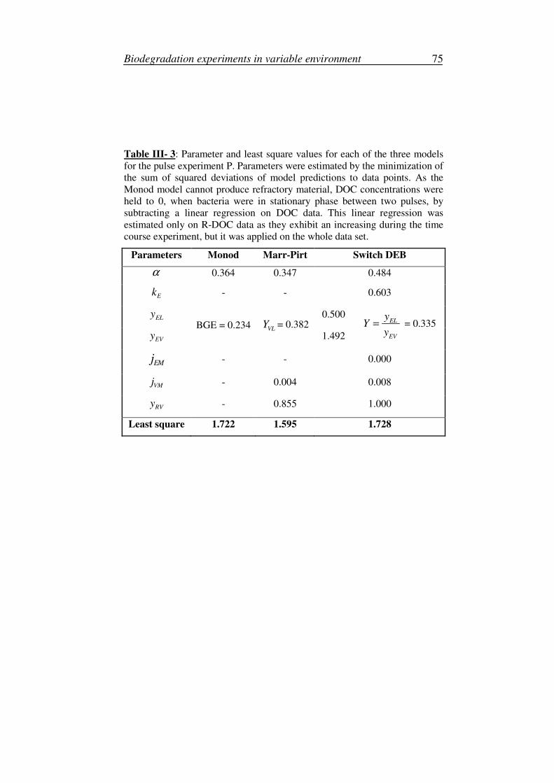
Biodegradation experiments in variable environment 75
Table III- 3: Parameter and least square values for each of the three models
for the pulse experiment P. Parameters were estimated by the minimization of
the sum of squared deviations of model predictions to data points. As the
Monod model cannot produce refractory material, DOC concentrations were
held to 0, when bacteria were in stationary phase between two pulses, by
subtracting a linear regression on DOC data. This linear regression was
estimated only on R-DOC data as they exhibit an increasing during the time
course experiment, but it was applied on the whole data set.
Parameters Monod Marr-Pirt Switch DEB
α 0.364 0.347 0.484
Ek - - 0.603
ELy 0.500
EVy BGE = 0.234 VL
Y = 0.382 1.492
EL
EV
yY
y= = 0.335
EMj - - 0.000
VMj - 0.004 0.008
RVy - 0.855 1.000
Least square 1.722 1.595 1.728
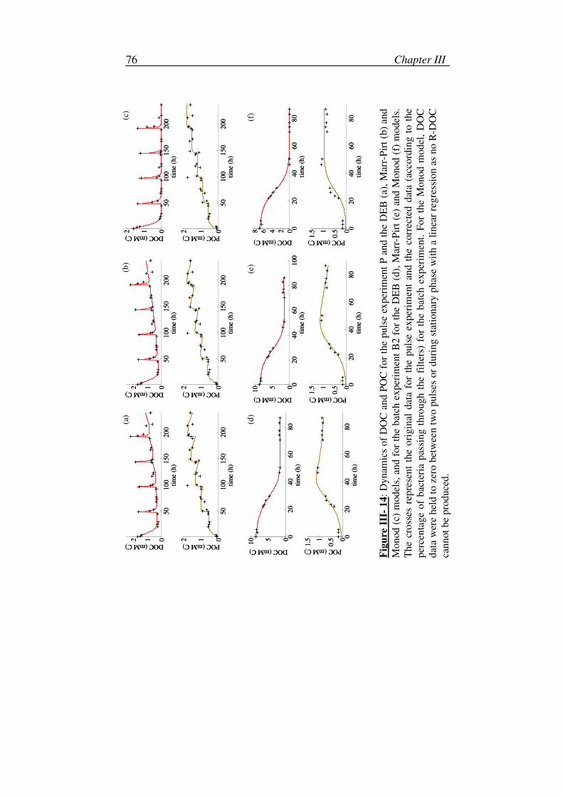
Chapter III 76
50
100
15
0200
012
tim
e (
h)
DOC (mM C)
50
100
15
0200
012
tim
e (
h)
POC (mM C)
50
100
150
200
012
DOC (mM C)
tim
e (h
)
50
100
150
200
012
tim
e (h
)
POC (mM C)
50
100
15
0200
012
tim
e (
h)
DOC (mM C)
50
100
15
0200
012
tim
e (
h)
POC (mM C)
02
040
60
80
05
10
tim
e (h
)
DOC (mM C)
02
040
60
80
0
0.51
1.5
tim
e (h
)
POC (mM C)
020
40
60
80
100
05
10
tim
e (
h)
DOC (mM C)
020
40
60
80
0
0.51
1.5
tim
e (
h)
POC (mM C)
020
40
60
80
02468
tim
e (
h)
DOC (mM C)
020
40
60
80
0
0.51
1.5
tim
e (
h)
POC (mM C)
(a)
(b)
(c)
(d)
(e)
(f)
50
100
15
0200
012
tim
e (
h)
DOC (mM C)
50
100
15
0200
012
tim
e (
h)
POC (mM C)
50
100
150
200
012
DOC (mM C)
tim
e (h
)
50
100
150
200
012
tim
e (h
)
POC (mM C)
50
100
15
0200
012
tim
e (
h)
DOC (mM C)
50
100
15
0200
012
tim
e (
h)
POC (mM C)
02
040
60
80
05
10
tim
e (h
)
DOC (mM C)
02
040
60
80
0
0.51
1.5
tim
e (h
)
POC (mM C)
020
40
60
80
100
05
10
tim
e (
h)
DOC (mM C)
020
40
60
80
0
0.51
1.5
tim
e (
h)
POC (mM C)
020
40
60
80
02468
tim
e (
h)
DOC (mM C)
020
40
60
80
0
0.51
1.5
tim
e (
h)
POC (mM C)
(a)
(b)
(c)
(d)
(e)
(f)
Fig
ure
III
- 1
4:
Dy
nam
ics
of
DO
C a
nd
PO
C f
or
the
pu
lse
exp
erim
ent
P a
nd
th
e D
EB
(a)
, M
arr-
Pir
t (b
) an
d
Mo
no
d (
c) m
od
els,
an
d f
or
the
bat
ch e
xp
erim
ent
B2
fo
r th
e D
EB
(d
), M
arr-
Pir
t (e
) an
d M
on
od
(f)
mo
del
s.
Th
e cr
oss
es r
epre
sen
t th
e o
rigin
al d
ata
for
the
puls
e ex
per
imen
t an
d t
he
corr
ecte
d d
ata
(acc
ord
ing
to
the
per
cen
tag
e o
f b
acte
ria
pas
sin
g t
hro
ug
h t
he
filt
ers)
fo
r th
e b
atch
ex
per
imen
t. F
or
the
Mo
nod
mo
del
, D
OC
dat
a w
ere
hel
d t
o z
ero
bet
wee
n t
wo
pu
lses
or
du
rin
g s
tati
on
ary
ph
ase
wit
h a
lin
ear
reg
ress
ion
as
no
R-D
OC
can
not
be
pro
duce
d.
Biodegradation experiments in variable environment 77
VI. Discussion
This study has allowed pointing out several processes. Firstly, we have
demonstrated that bacteria are able to produce refractory material. However,
the nature of this material is unknown: it could consist of cell wall,
suggesting that bacteria are a source of DOM and that bacteria-derived
organic matter can be preserved for long periods (Nagata 2000), or it could
consist of exopolysacharrides (EPS) as this bacterial strain produce it during
the stationary phase (Raguénès et al. 1997). Chemical analyses are needed to
identify the nature of this refractory material. To be sure that the studied
system is fully limited by OC and not by a nutrient, it could be interesting to
measure the pyruvate as well as the total DOC concentration. Such
information could help us to understand whether the remaining DOC is only
refractory or if it is made up of a part of not assimilated substrate. We could
also measure the nutrient concentrations to follow their dynamics and
eventually include them in models. However, this would complicate the
experimental design by increasing the culture volume that needed
considerably. An alternative would be the use of chemostats with a constant
culture volume. The experimental design should be adjusted to allow the
introduction of the pulses, for example by changing the dilution rate.
The respiration measurements allowed the study of maintenance during
the stationary phase. The Monod model is not suitable for this purpose.
Indeed, it considers that a proportion BGE is used for the growth, and that the
remaining proportion (1-BGE) is used for the respiration. However, when
considering the equations, substrate concentration (L) equal to zero would
imply that the respiration (which amounts to (1-BGE) L MV, where MV
stands for the bacterial biomass) is also null. This result is inconsistent with
our experimental results. The choice of a model is highly influenced by the
available data. Indeed, if our experiments stopped after the growth phase and
if we did not measure the respiration, we would notice that the Monod model
is sufficient for this experiment. In this study, Marr-Pirt and DEB models are
almost equivalent in terms of dynamics and of BGE estimations. However,
by including nutrient measurements for example, we could appreciate the
relevance of mechanistic approach, as the DEB theory, considering processes
as the assimilation, maintenance and growth of each element. It has been
demonstrated that when considering a food chain with a bacteria, fed on
glucose, and a predator, the Monod and Marr-Pirt models are not able to
reproduce experimental dynamics, whereas the DEB model is (Kooi &
Kooijman 1994). Consequently, experimental efforts and developments are
necessary to assess bacterial processes that should be included in models.
Chapter III 78
The P experiment and especially the respiration measurements, showed
the versatility of bacterial metabolism, which is difficult to observe in
constant conditions. We may introduce the notion of population
synchronisation as bacteria are constrained by the presence or absence of
food. This synchronisation may be due to several factors, such as the stress
generated by absence of substrate and the large energy requirement for
maintenance. Consequently, all bacteria become active at the same moment
to assimilate the substrate and to grow, and cells continue maintenance when
the substrate has totally disappeared. This metabolic flexibility is necessary
to cope with the vicissitudes of a largely oligotrophic and ever-changing
environment, and may result from the uncoupling of anabolic and catabolic
processes (del Giorgio & Cole 1998). We may believe that the situation is the
same in natural seawater, as food is not continuously available (Hanegraaf &
Kooi 2002) and bacteria may be faced with long periods of absence of one or
more nutrients (Konopka 1999) and with short periods of high substrate
availability. Thus, by carrying out batch biodegradation experiments using in
situ samples, bacteria may be in one or another situation. The resulting BGE
are of course affected by the temporal variation of substrate availability. We
consequently have to be very cautious when comparing BGE from different
study sites and periods, without considering the “story” of the water mass.
We also observed a highly significant autocorrelation between the
various bacterial variables (POC, bacterial density and OD), especially for
the batch experiments B1 and B2. It may be possible that calibration of two
variables on the third would reduce the experimental cost and work
considerably. For example, OD measurements do not require a large culture
volume (2 cm3 against 10 to 100 cm
3 for POC measurements) and are really
fast and not expensive compared to POC and bacterial density measurements.
However, it seems that this correlation is less accurate during the stationary
phase compared to other growth phases, justifying that this kind of
formulation should be applied cautiously. Moreover, three models have been
used in this study to describe DOC and bacterial dynamics, and we have
demonstrated that the Monod model is inaccurate for these data sets. Marr-
Pirt and DEB models can thus be used in further work to determine critical
variables and parameters to be measured.
On the other hand, the numerous variables measured also permitted to
estimate the carbon content per bacteria, often called carbon conversion
factor (CCF). This CCF is often considered constant and used to convert
bacterial density into bacterial biomass-carbon. The mean CCF for marine
bacteria is often considered to be 20 fgC bacterium-1
(Lee & Fuhrman 1987).
However, our study clearly showed that this CCF is not constant but varies
Biodegradation experiments in variable environment 79
during the time course of the experiment. Indeed, in the experiment B2, CCF
decreased rapidly from 450 to 30 fgC bacterium-1
(38 to 3 fmolC bacterium-1
)
during the first lag phase, and then is quite stable during the rest of the
experiment (Figure III-11). In the P experiment, the CCF also decreased from
180 to 60 fgC bacterium-1
(15 to 5 fmolC bacterium-1
) during the lag and
exponential growth phases, and increased after each pulse (Figure III-11).
The variation of the carbon content per cell has already been reported
(Ducklow & Carlson 1992), being larger during growth phases than during
stationary phase (Vrede et al. 2002). Due to the huge variation of the CCF
during the several growth phases, the use of a constant CCF to deduce
bacterial biomass-C from bacterial density should be avoided. By using a
CCF of 20 fgC bacterium-1
for the first steps of the experiment B2, the error
could be higher than 200 %.
The calibration of the Monod, Marr-Pirt and DEB models on these data
sets demonstrated the weakness of the Monod model to reproduce this kind
of dynamics. The presence of the maintenance process is necessary to assess
these bacterial dynamics. However, it seems that the formulation of the
maintenance process has little impact on the model outputs. Nevertheless, the
DEB model, due to its mechanistic formulation, is more flexible than the
Marr-Pirt model and is able to apply to more situations. The maintenance
from the reserve has more importance in the B2 experiment than in the P
experiment. Indeed, the parameter EM
j is negligibly small in the pulse
experiment whereas it equals 0.021 h-1
in the batch B2 experiment (Tables
III-2 and III-3). Contrary to the pulse experiment, the maintenance from
reserve is higher than maintenance from the structure in the batch experiment
(EM
j is more than three times higher than VMj ) (Table III-2). If the pulse
experiment was realised with the initial conditions of the batch experiment
B2 and with a longer pulse period, the Marr-Pirt model might have been
unable to reproduce experimental dynamics as it does not comprise
maintenance from reserve which is no more negligible (Figure III-15).
Consequently, a mechanistic model like the DEB model may be useful in
other conditions than that used in our pulse experiment, and may thus show
dynamical differences with the Marr-Pirt model.
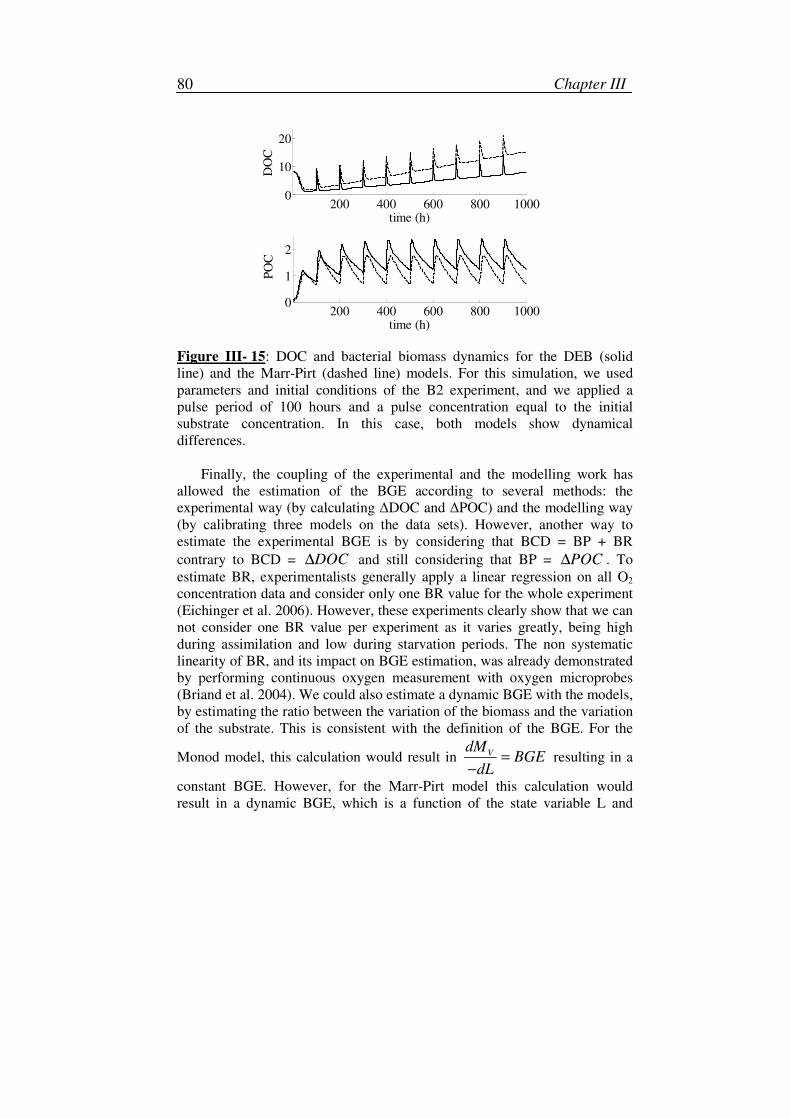
Chapter III 80
200 400 600 800 10000
10
20
time (h)
DO
C
200 400 600 800 10000
1
2
time (h)
PO
C
Figure III- 15: DOC and bacterial biomass dynamics for the DEB (solid
line) and the Marr-Pirt (dashed line) models. For this simulation, we used
parameters and initial conditions of the B2 experiment, and we applied a
pulse period of 100 hours and a pulse concentration equal to the initial
substrate concentration. In this case, both models show dynamical
differences.
Finally, the coupling of the experimental and the modelling work has
allowed the estimation of the BGE according to several methods: the
experimental way (by calculating ∆DOC and ∆POC) and the modelling way
(by calibrating three models on the data sets). However, another way to
estimate the experimental BGE is by considering that BCD = BP + BR
contrary to BCD = DOC∆ and still considering that BP = POC∆ . To
estimate BR, experimentalists generally apply a linear regression on all O2
concentration data and consider only one BR value for the whole experiment
(Eichinger et al. 2006). However, these experiments clearly show that we can
not consider one BR value per experiment as it varies greatly, being high
during assimilation and low during starvation periods. The non systematic
linearity of BR, and its impact on BGE estimation, was already demonstrated
by performing continuous oxygen measurement with oxygen microprobes
(Briand et al. 2004). We could also estimate a dynamic BGE with the models,
by estimating the ratio between the variation of the biomass and the variation
of the substrate. This is consistent with the definition of the BGE. For the
Monod model, this calculation would result in VdM
BGEdL
=
−
resulting in a
constant BGE. However, for the Marr-Pirt model this calculation would
result in a dynamic BGE, which is a function of the state variable L and
Biodegradation experiments in variable environment 81
amounts to V VMVL
dM jY
dL Lα
= −
−
. For the DEB model, the BGE is also variable
and amounts to E EV V EMEL
dM y dM jy
dL Lα
+= −
−
when E E EM Vk M j M>
and to a more complex function in the other case. This dynamic estimation is
also possible for the experimental BGE by calculating BGE from two
consecutive data points. But for instance the variability between data does not
allow a sufficient sensitivity to investigate such estimation. Nevertheless, it
would be very interesting to compare these BGE for the different
experiments and models, but we should previously choose a criterion for
comparison as we can no longer compare single values but dynamics.
Moreover, we would also have to solve some numerical problems as when L
values approach 0, the dynamic BGE tends to infinity.
The values of the four constant BGE (one experimental BGE and three
BGE resulting from models) differed, but it always results that the BGE is
higher in the pulse than in the batch experiment. We can thus state that
bacteria are more efficient in a transient than in a constant environment
(Poggiale et al. 2005). It seems that they are unable to grow efficiently when
a large amount of substrate is present, whereas there growth is stimulated
when the same amount of substrate is brought periodically.
As the parameter α , the ratio between the maximum absorption rate
mLAj and the half-saturation constant K , is also always higher for the pulse
experiment (Tables III-2 and III-3), we can assume that bacteria also increase
their maximum assimilation rate and/or increase their affinity to the substrate
(decrease of K) in the pulse experiment. This is consistent with the fact that
bacteria are faced with apparent “long” periods of absence of substrate, and
that they subsequently have to increase their affinity to the substrate in order
to increase their growth efficiency. The presence of two K systems has still
been mentioned (Baxter & Sieburth 1984), where the low K system is
constitutive and saturable, whereas the high K system may result from
facilitated diffusion coupled with extracellular polymeric carbohydrate
production. This hypothesis is consistent with our experiments as high
affinities are observed in the P experiment showing the maximum products
formation, which could correspond to EPS. Another hypothesis which might
explain higher BGE values for the pulse experiment is by considering the
competition. We can consider a ratio δ between the amount of available
substrate and the bacterial density. Both experiments started with the same
bacterial density but the substrate concentration was 5 times higher in the
Chapter III 82
batch experiment B2. Consequently, δ was higher in the B2 experiment
which indicates a high substrate amount per bacterium. Thus, the competition
for the substrate is negligible and bacteria do not need to increase their BGE
or substrate affinity. By contrast, since the beginning of the pulse experiment,
δ is small. Moreover, bacterial density increased in the time course of the
experiment, and we periodically added the same substrate concentration in
the culture. Consequently, δ decreased during the experiment, leading to a
strong competition between bacteria which need to increase their BGE and
affinity to the substrate. As bacteria are in strong limitation between two
pulses, they also assimilate very rapidly each substrate pulse, which supports
the increase of mLA
j .
VII. Conclusion
Numerous studies have investigated how environmental factors
influenced the BGE (del Giorgio & Cole 1998). It was still demonstrated that
BGE is influenced by DOC quality in term of molecular weight (Amon &
Benner 1996), DOC chemical nature (Carlson & Ducklow 1996, Cherrier et
al. 1996, Cherrier & Bauer 2004), substrate C:N ratio (Goldman et al. 1987),
distance from the seashore (del Giorgio & Cole 1998, La Ferla et al. 2005),
season (Reinthaler & Herndl 2005, Eichinger et al. 2006) and depth
(Eichinger et al. 2006). However, there have been only few investigations
dealing with daily and detailed seasonal variation of natural BGE (del
Giorgio & Cole 1998). We have demonstrated that the temporal variation in
substrate availability influence the BGE greatly, which may be two times
higher in a pulse than in constant experimental conditions. This outcome may
have great impact on knowledge resulting from the long effort on BGE
determination. Indeed, to determine BGE we need to uncouple DOC
production from its consumption, however the time and space variability of
DOC distribution in field makes BGE highly variable. More experiments are
required to confirm our results, for example by improving the protocol by
measuring also nutrient concentration and by progressively improving the
protocol to incorporate the DOC source more naturally. However, we should
still consider pulse load of substrate or other kinds of variable inputs. The
outcome of this study is even more important knowing that model
formulation and parameter estimation from experimental dynamics are often
used in global models to investigate the oceanic carbon cycle.
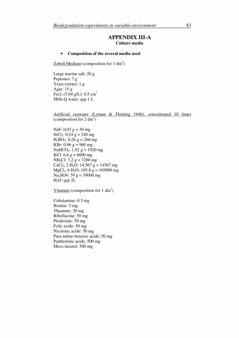
Biodegradation experiments in variable environment 83
APPENDIX III-A Culture media
• Composition of the several media used
Zobell Medium (composition for 1 dm
3)
Large marine salt: 20 g
Peptones: 7 g
Yeast extract: 1 g
Agar: 15 g
Fecl3 (5.04 g/L): 0.5 cm3
Milli-Q water: qsp 1 L
Artificial seawater (Lyman & Fleming 1940), concentrated 10 times
(composition for 2 dm3)
NaF: 0,03 g = 30 mg
SrCl2: 0,24 g = 240 mg
H3BO3: 0,26 g = 260 mg
KBr: 0,96 g = 960 mg
NaHCO3: 1,92 g = 1920 mg
KCl: 6,6 g = 6600 mg
NH4Cl: 7,2 g = 7200 mg
CaCl2, 2 H2O: 14.567 g = 14567 mg
MgCl2, 6 H2O: 105.8 g = 105800 mg
Na2SO4: 39 g = 39000 mg
H2O: qsp 2L
Vitamins (composition for 1 dm3)
Cobalamine: 0.5 mg
Biotine: 5 mg
Thiamine: 50 mg
Riboflavine: 50 mg
Piridoxine: 50 mg
Folic acide: 50 mg
Nicotinic acide: 50 mg
Para amino benzoic acide: 50 mg
Panthoténic acide: 500 mg
Meso-inisitol: 500 mg
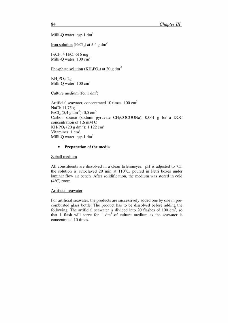
Chapter III 84
Milli-Q water: qsp 1 dm3
Iron solution (FeCl2) at 5.4 g dm-3
FeCl2, 4 H2O: 616 mg
Milli-Q water: 100 cm3
Phosphate solution (KH2PO4) at 20 g dm-3
KH2PO4: 2g
Milli-Q water: 100 cm3
Culture medium (for 1 dm3)
Artificial seawater, concentrated 10 times: 100 cm3
NaCl: 11,75 g
FeCl2 (5,4 g dm-3
): 0,5 cm3
Carbon source (sodium pyruvate CH3COCOONa): 0,061 g for a DOC
concentration of 1,6 mM C
KH2PO4 (20 g dm-3
): 1,122 cm3
Vitamines: 1 cm3
Milli-Q water: qsp 1 dm3
• Preparation of the media
Zobell medium
All constituents are dissolved in a clean Erlenmeyer. pH is adjusted to 7.5,
the solution is autoclaved 20 min at 110°C, poured in Petri boxes under
laminar flow air bench. After solidification, the medium was stored in cold
(4°C) room.
Artificial seawater
For artificial seawater, the products are successively added one by one in pre-
combusted glass bottle. The product has to be dissolved before adding the
following. The artificial seawater is divided into 20 flashes of 100 cm3, so
that 1 flash will serve for 1 dm3 of culture medium as the seawater is
concentrated 10 times.
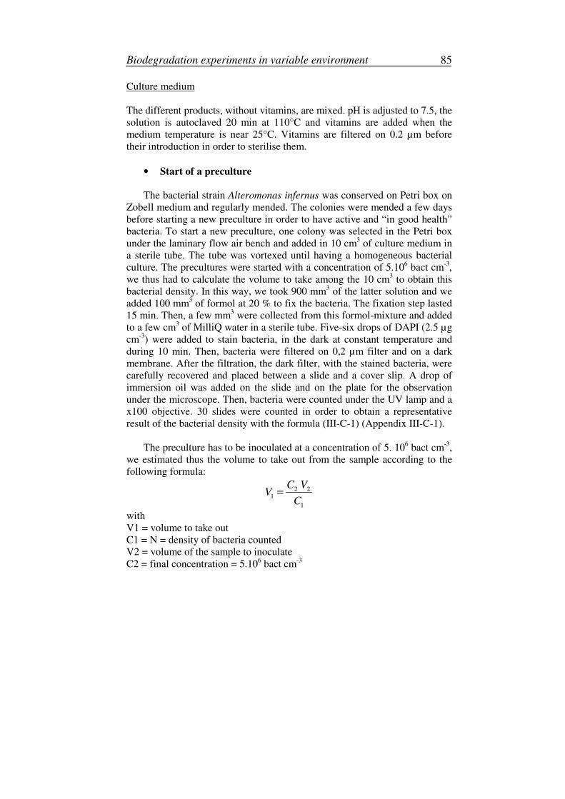
Biodegradation experiments in variable environment 85
Culture medium
The different products, without vitamins, are mixed. pH is adjusted to 7.5, the
solution is autoclaved 20 min at 110°C and vitamins are added when the
medium temperature is near 25°C. Vitamins are filtered on 0.2 µm before
their introduction in order to sterilise them.
• Start of a preculture
The bacterial strain Alteromonas infernus was conserved on Petri box on
Zobell medium and regularly mended. The colonies were mended a few days
before starting a new preculture in order to have active and “in good health”
bacteria. To start a new preculture, one colony was selected in the Petri box
under the laminary flow air bench and added in 10 cm3 of culture medium in
a sterile tube. The tube was vortexed until having a homogeneous bacterial
culture. The precultures were started with a concentration of 5.106 bact cm
-3,
we thus had to calculate the volume to take among the 10 cm3 to obtain this
bacterial density. In this way, we took 900 mm3 of the latter solution and we
added 100 mm3 of formol at 20 % to fix the bacteria. The fixation step lasted
15 min. Then, a few mm3 were collected from this formol-mixture and added
to a few cm3 of MilliQ water in a sterile tube. Five-six drops of DAPI (2.5 µg
cm-3
) were added to stain bacteria, in the dark at constant temperature and
during 10 min. Then, bacteria were filtered on 0,2 µm filter and on a dark
membrane. After the filtration, the dark filter, with the stained bacteria, were
carefully recovered and placed between a slide and a cover slip. A drop of
immersion oil was added on the slide and on the plate for the observation
under the microscope. Then, bacteria were counted under the UV lamp and a
x100 objective. 30 slides were counted in order to obtain a representative
result of the bacterial density with the formula (III-C-1) (Appendix III-C-1).
The preculture has to be inoculated at a concentration of 5. 106 bact cm
-3,
we estimated thus the volume to take out from the sample according to the
following formula:
2 21
1
C VV
C=
with
V1 = volume to take out
C1 = N = density of bacteria counted
V2 = volume of the sample to inoculate
C2 = final concentration = 5.106 bact cm
-3

Chapter III 86
We then introduced the volume V1, with the bacteria, in the new medium
V2 that had the same composition. This preculture is incubated in the dark at
25°C during 3 days, in order to start the culture with starved bacteria.
• Start of a culture
The cultures were started from the previous preculture. The inoculation
scheme is almost the same than for the preculture. Indeed, a few cm3 of this
preculture was collected, and the DAPI stained bacteria were counted by
epifluorescent microscopy. After bacterial addition, the culture was
homogenised and this time corresponded to the time 0 of the experiment.
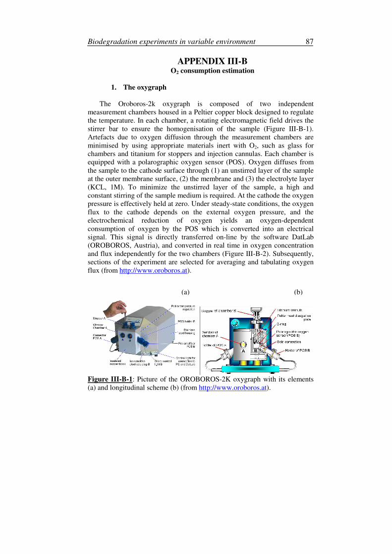
Biodegradation experiments in variable environment 87
APPENDIX III-B O2 consumption estimation
1. The oxygraph
The Oroboros-2k oxygraph is composed of two independent
measurement chambers housed in a Peltier copper block designed to regulate
the temperature. In each chamber, a rotating electromagnetic field drives the
stirrer bar to ensure the homogenisation of the sample (Figure III-B-1).
Artefacts due to oxygen diffusion through the measurement chambers are
minimised by using appropriate materials inert with O2, such as glass for
chambers and titanium for stoppers and injection cannulas. Each chamber is
equipped with a polarographic oxygen sensor (POS). Oxygen diffuses from
the sample to the cathode surface through (1) an unstirred layer of the sample
at the outer membrane surface, (2) the membrane and (3) the electrolyte layer
(KCL, 1M). To minimize the unstirred layer of the sample, a high and
constant stirring of the sample medium is required. At the cathode the oxygen
pressure is effectively held at zero. Under steady-state conditions, the oxygen
flux to the cathode depends on the external oxygen pressure, and the
electrochemical reduction of oxygen yields an oxygen-dependent
consumption of oxygen by the POS which is converted into an electrical
signal. This signal is directly transferred on-line by the software DatLab
(OROBOROS, Austria), and converted in real time in oxygen concentration
and flux independently for the two chambers (Figure III-B-2). Subsequently,
sections of the experiment are selected for averaging and tabulating oxygen
flux (from http://www.oroboros.at).
Figure III-B-1: Picture of the OROBOROS-2K oxygraph with its elements
(a) and longitudinal scheme (b) (from http://www.oroboros.at).
(a) (b)
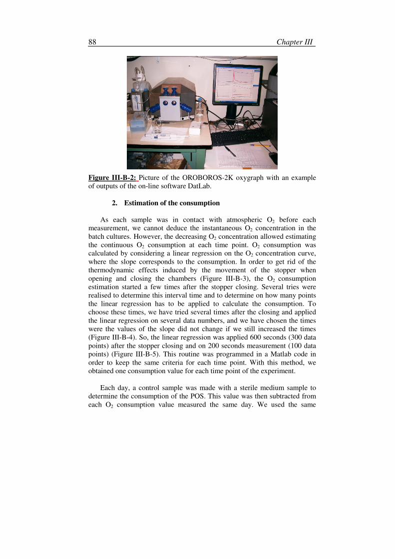
Chapter III 88
Figure III-B-2: Picture of the OROBOROS-2K oxygraph with an example
of outputs of the on-line software DatLab.
2. Estimation of the consumption
As each sample was in contact with atmospheric O2 before each
measurement, we cannot deduce the instantaneous O2 concentration in the
batch cultures. However, the decreasing O2 concentration allowed estimating
the continuous O2 consumption at each time point. O2 consumption was
calculated by considering a linear regression on the O2 concentration curve,
where the slope corresponds to the consumption. In order to get rid of the
thermodynamic effects induced by the movement of the stopper when
opening and closing the chambers (Figure III-B-3), the O2 consumption
estimation started a few times after the stopper closing. Several tries were
realised to determine this interval time and to determine on how many points
the linear regression has to be applied to calculate the consumption. To
choose these times, we have tried several times after the closing and applied
the linear regression on several data numbers, and we have chosen the times
were the values of the slope did not change if we still increased the times
(Figure III-B-4). So, the linear regression was applied 600 seconds (300 data
points) after the stopper closing and on 200 seconds measurement (100 data
points) (Figure III-B-5). This routine was programmed in a Matlab code in
order to keep the same criteria for each time point. With this method, we
obtained one consumption value for each time point of the experiment.
Each day, a control sample was made with a sterile medium sample to
determine the consumption of the POS. This value was then subtracted from
each O2 consumption value measured the same day. We used the same
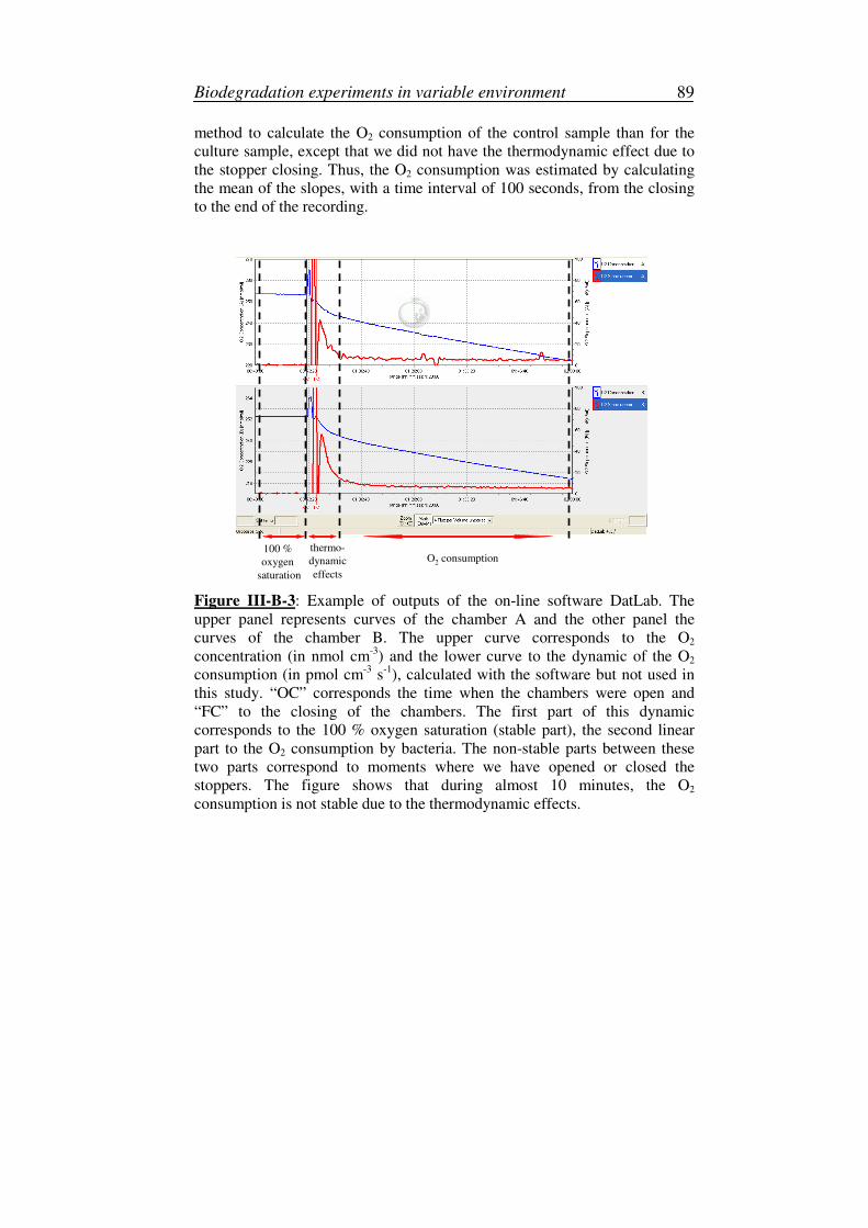
Biodegradation experiments in variable environment 89
method to calculate the O2 consumption of the control sample than for the
culture sample, except that we did not have the thermodynamic effect due to
the stopper closing. Thus, the O2 consumption was estimated by calculating
the mean of the slopes, with a time interval of 100 seconds, from the closing
to the end of the recording.
100 %
oxygen
saturation
thermo-
dynamic
effects
O2 consumption
Figure III-B-3: Example of outputs of the on-line software DatLab. The
upper panel represents curves of the chamber A and the other panel the
curves of the chamber B. The upper curve corresponds to the O2
concentration (in nmol cm-3
) and the lower curve to the dynamic of the O2
consumption (in pmol cm-3
s-1
), calculated with the software but not used in
this study. “OC” corresponds the time when the chambers were open and
“FC” to the closing of the chambers. The first part of this dynamic
corresponds to the 100 % oxygen saturation (stable part), the second linear
part to the O2 consumption by bacteria. The non-stable parts between these
two parts correspond to moments where we have opened or closed the
stoppers. The figure shows that during almost 10 minutes, the O2
consumption is not stable due to the thermodynamic effects.
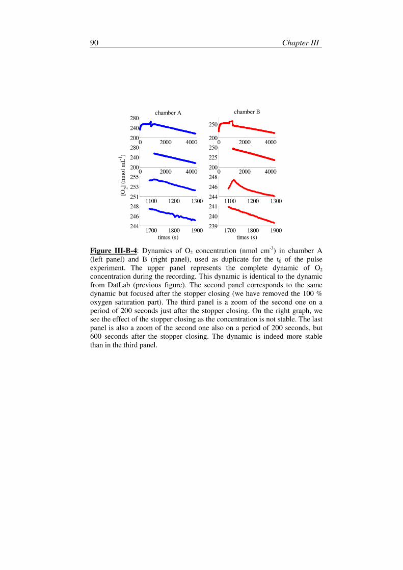
Chapter III 90
0 2000 4000200
240
280chamber A
0 2000 4000200
250
chamber B
0 2000 4000200
240
280
0 2000 4000200
225
250
1100 1200 1300251
253
255
[O2]
(nm
ol
mL-1
)
1100 1200 1300244
246
248
1700 1800 1900244
246
248
times (s)1700 1800 1900
239
240
241
times (s)
Figure III-B-4: Dynamics of O2 concentration (nmol cm-3
) in chamber A
(left panel) and B (right panel), used as duplicate for the t0 of the pulse
experiment. The upper panel represents the complete dynamic of O2
concentration during the recording. This dynamic is identical to the dynamic
from DatLab (previous figure). The second panel corresponds to the same
dynamic but focused after the stopper closing (we have removed the 100 %
oxygen saturation part). The third panel is a zoom of the second one on a
period of 200 seconds just after the stopper closing. On the right graph, we
see the effect of the stopper closing as the concentration is not stable. The last
panel is also a zoom of the second one also on a period of 200 seconds, but
600 seconds after the stopper closing. The dynamic is indeed more stable
than in the third panel.
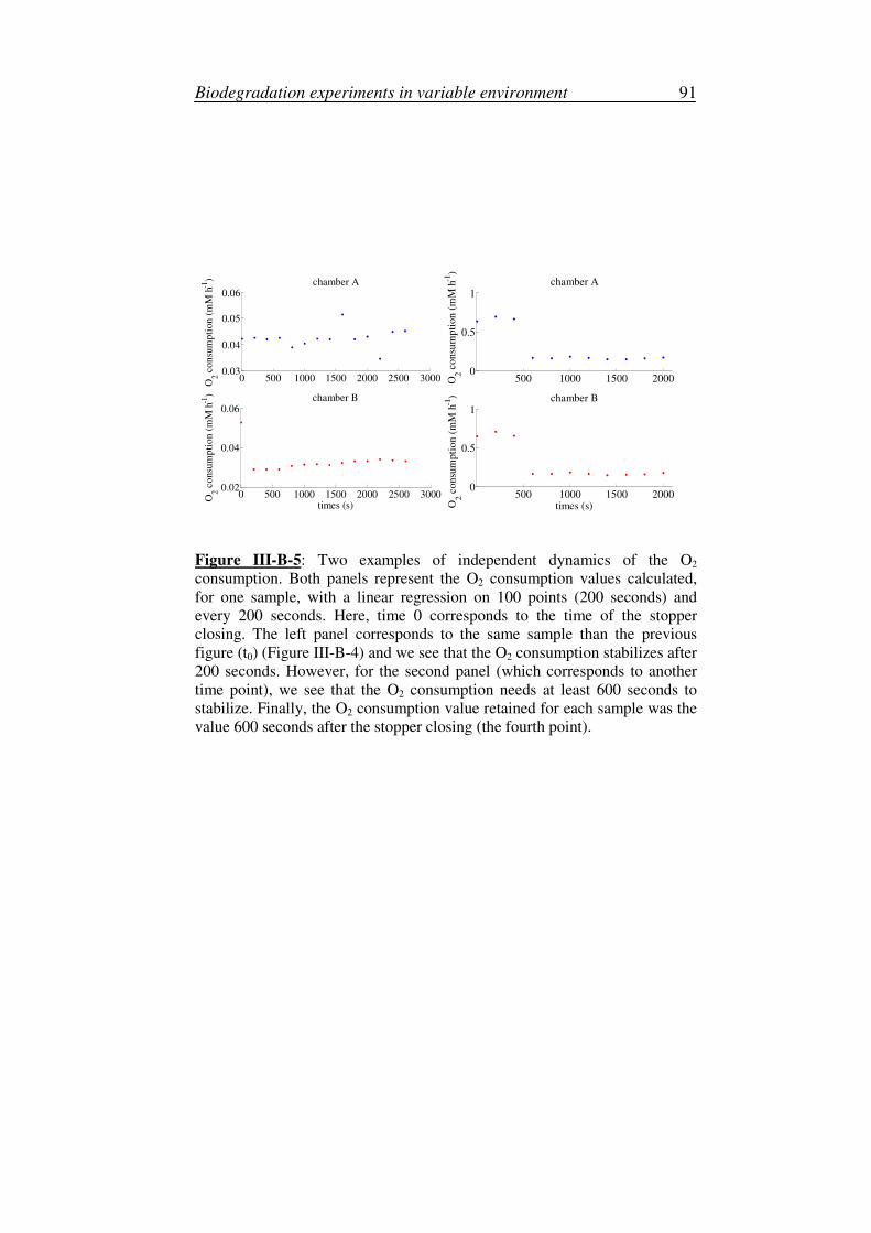
Biodegradation experiments in variable environment 91
0 500 1000 1500 2000 2500 30000.03
0.04
0.05
0.06
O2 c
on
sum
pti
on
(m
M h
-1) chamber A
0 500 1000 1500 2000 2500 30000.02
0.04
0.06
O2 c
onsu
mp
tio
n (
mM
h-1
)
times (s)
chamber B
500 1000 1500 20000
0.5
1
O2 c
on
sum
pti
on
(m
M h
-1)
chamber A
500 1000 1500 20000
0.5
1
O2 c
on
sum
pti
on
(m
M h
-1)
times (s)
chamber B
Figure III-B-5: Two examples of independent dynamics of the O2
consumption. Both panels represent the O2 consumption values calculated,
for one sample, with a linear regression on 100 points (200 seconds) and
every 200 seconds. Here, time 0 corresponds to the time of the stopper
closing. The left panel corresponds to the same sample than the previous
figure (t0) (Figure III-B-4) and we see that the O2 consumption stabilizes after
200 seconds. However, for the second panel (which corresponds to another
time point), we see that the O2 consumption needs at least 600 seconds to
stabilize. Finally, the O2 consumption value retained for each sample was the
value 600 seconds after the stopper closing (the fourth point).
Chapter III 92
APPENDIX III-C Cell counts
1. Microscopy
For each slide, 30 fields were counted, and the bacterial abundance N (in
cell cm-3
) was estimated according to the following formula:
2
preparedmean
grid filtered sample
Vn D πN
S V V= (III-C-1)
with
nmean = average bacterial number per field
Sgrid = surface of the count grid = 6400 µm2 (10000 µm
2 ) if the microscope
used was the Olympus BH 2 (Olympus BX 61)
D = diameter of the filtration surface = 15500 µm (18300 µm ) if the filterer
used was a turret (multiposition rosette)
Vfiltred = volume of the filtered sample
Vprepared = prepared volume (with formol) = 1000 mm3
Vsample = total volume of the sample (without formol) = 900 mm3
2. Flow cytometry
The flow cytometer MoFlo cell sorter is equipped with a water cooled
Argon laser providing a 352 nm (UV) and a 488 nm (blue) laser beam set up
on a regulated 50 mW outpout power on UV. Three optical properties were
measured for each single particle analyzed. Two light scatter intensities based
on the 488 nm laser beam were measured, namely forward angle light scatter
(related to the particle size) and right angle light scatter (related to cell
structure and shape). The bacteria fluorescence induced by the DAPI after
nucleic acid staining and UV excitation was also specifically recorded using
a 405 ± 30 nm band pass-filter placed just in front of the photodetector. All
the parameters were acquired in logarithmic scale, and the trigger acquisition
was based on the right angle light scatter intensity in order to detect all the
particles in the sample (bacteria, debris). The data were acquired in real time
and list-mode using the SUMMIT 4.3 software (Dako, Dk). Flow cytometry
data files (in Flow Cytometry Standard 3.0 format) were also analyzed using
the same software.
In order to avoid doublets and hard coincidences, samples were diluted in
sterile medium in order to keep a flow rate lower than 8,000 events analysed

Biodegradation experiments in variable environment 93
per second, a mandatory condition to ensure accurate counting. The sheath
tank of the flow cytometer was filled with 0.2 µm filtered distilled water.
Sheath pressure was kept constant at 60.0 PSI, and sample pressure at 60.1
PSI. Analyses were performed during 1 minute. The exact volume analyzed
was derived from a preliminary calibration phase during which a sample was
weighed before and after a 3 minutes analysis in order to determine the
average flow rate (in mm3 s
-1). The procedure is repeated 3 times and the
average flow rate is calculated. Bacteria were optically resolved from the
cytogram Right angle light scatter (au) versus DAPI fluorescence intensity
(au). A manual region was drawn around them and the SUMMIT software
automatically displayed the bacteria count. Dividing the bacteria count by the
volume analyzed provides the cell abundance.

94
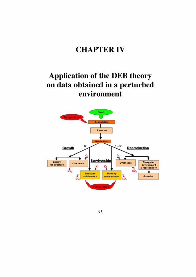
95
CHAPTER IV
Application of the DEB theory
on data obtained in a perturbed
environment
Chapter IV 96
Abstract
We developed a model for the biodegradation of organic compounds
based on a set of data from an experiment with pulse donation of substrate.
Experiments were realised with a monospecific bacterial strain and a unique
carbon substrate. The mechanistic model has a reserve compartment as well
as two maintenance terms and represents an application of the Dynamic
Energy Budget (DEB) theory. The measured variables were the dissolved
organic carbon (DOC) corresponding to the substrate concentration in
addition to other DOC forms, and the particulate organic carbon (POC)
corresponding to the carbon bacterial biomass. The model, comprising 4 state
variables and 7 parameters, matches the data very well, but the complexity of
this model makes it difficult to implement it in ecosystem models. We
showed that the DEB model can be simplified to a model with two state
variables and a logistic-like growth, with a variable carrying capacity. The
other two state variables of the DEB model reduce to functions of the state
variables of the simplified model. Using parameter values that correspond to
the experimental results, simulations of the DOC and POC kinetics for the
DEB model and its simplification are similar. The reduction of the DEB
model to a model with two state variables offers the advantage that the
reduced model can be numerically integrated with simplicity. Computational
costs are greatly decreased, which is of great interest for further coupling of
this bacterial growth model with biogeochemical and hydrodynamical
transport models. Moreover, this simplification gives a mechanistic basis to
the logistic equation.
Modelling bacterial growth with DEB theory 97
I. The DEB theory for micro-organisms
1. General concepts
The Dynamic Energy Budget (DEB; (Kooijman 2000)) theory provides
rules for uptake and use of energy by organisms. It exploits conservation
laws and stoichiometric constraints. Energy and mass fluxes through the
organisms and their surroundings are central in the DEB framework. One
advantage of this theory is that, due to its mechanistic basis, small changes
are sufficient to adapt the model from one to another organism.
The DEB theory assumes that an organism is partitioned into a reserve
and a structural compartment. The structural biomass is continuously
degraded and reconstituted, whereas the reserve material is used and
replenished. The DEB theory focuses on three major processes: assimilation,
maintenance and growth. Food (substrate) uptake is proportional to the
surface area of the organism. The food (or substrate) is always assimilated in
the reserve compartment, and reserves are subsequently used to pay the
several costs. For each species of organism, a fixed part κ of this catabolic
flux is used to pay somatic maintenance and growth, the remaining (1- κ) is
used for development and/or reproduction. This law is called the “κ rule” in
the DEB context. Typically three life stages are delineated, embryos don’t
feed or reproduce, juveniles feed but don’t reproduce and adults feed and
reproduce. For micro-organisms, which classify as juvenile, somatic and
maturity maintenance can be combined and growth and maturation can be
combined, which makes that we can set κ =1 without loss of generality.
Maintenance has always priority above growth, thus growth stops if all the
mobilised reserve for maintenance + growth is used for maintenance. The
latter is paid to maintain the integrity of the cells and to maintain gradients
across the cell membrane. Maintenance costs are assumed to be proportional
to the structural volume. The specific growth costs are assumed to be
constant during the life of an organism. This hypothesis implies that the
structural biomass has a constant chemical composition: this is known as the
strong homeostasis assumption in the DEB framework. It is also assumed
that reserves respect the strong homeostasis assumption. However, since the
proportion of structure and reserve can change during the life of an organism,
the macro-chemical composition of the whole organism can vary.
DEB theory provides also rules for the coupling between energy and
mass fluxes. Experimental observations are mostly made on mass. Thus, we
need robust rules to compare observations to model outputs. Models resulting
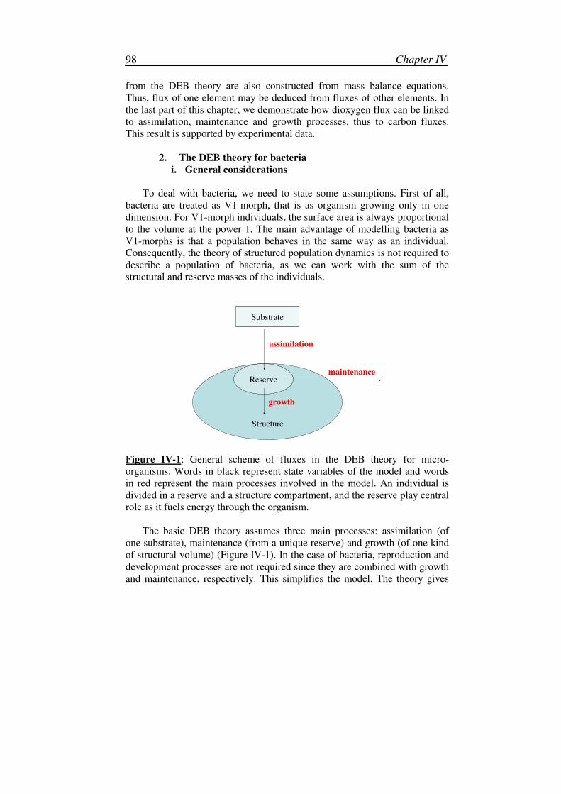
Chapter IV 98
from the DEB theory are also constructed from mass balance equations.
Thus, flux of one element may be deduced from fluxes of other elements. In
the last part of this chapter, we demonstrate how dioxygen flux can be linked
to assimilation, maintenance and growth processes, thus to carbon fluxes.
This result is supported by experimental data.
2. The DEB theory for bacteria
i. General considerations
To deal with bacteria, we need to state some assumptions. First of all,
bacteria are treated as V1-morph, that is as organism growing only in one
dimension. For V1-morph individuals, the surface area is always proportional
to the volume at the power 1. The main advantage of modelling bacteria as
V1-morphs is that a population behaves in the same way as an individual.
Consequently, the theory of structured population dynamics is not required to
describe a population of bacteria, as we can work with the sum of the
structural and reserve masses of the individuals.
Reserve
Substrate
Structure
assimilation
maintenance
growth
Figure IV-1: General scheme of fluxes in the DEB theory for micro-
organisms. Words in black represent state variables of the model and words
in red represent the main processes involved in the model. An individual is
divided in a reserve and a structure compartment, and the reserve play central
role as it fuels energy through the organism.
The basic DEB theory assumes three main processes: assimilation (of
one substrate), maintenance (from a unique reserve) and growth (of one kind
of structural volume) (Figure IV-1). In the case of bacteria, reproduction and
development processes are not required since they are combined with growth
and maintenance, respectively. This simplifies the model. The theory gives
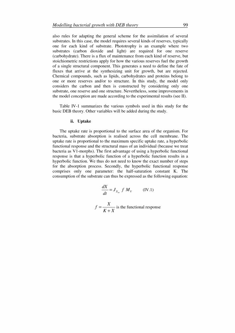
Modelling bacterial growth with DEB theory 99
also rules for adapting the general scheme for the assimilation of several
substrates. In this case, the model requires several kinds of reserves, typically
one for each kind of substrate. Phototrophy is an example where two
substrates (carbon dioxide and light) are required for one reserve
(carbohydrate). There is a flux of maintenance from each kind of reserve, but
stoichiometric restrictions apply for how the various reserves fuel the growth
of a single structural component. This generates a need to define the fate of
fluxes that arrive at the synthesizing unit for growth, but are rejected.
Chemical compounds, such as lipids, carbohydrates and proteins belong to
one or more reserves and/or to structure. In this study, the model only
considers the carbon and then is constructed by considering only one
substrate, one reserve and one structure. Nevertheless, some improvements in
the model conception are made according to the experimental results (see II).
Table IV-1 summarizes the various symbols used in this study for the
basic DEB theory. Other variables will be added during the study.
ii. Uptake
The uptake rate is proportional to the surface area of the organism. For
bacteria, substrate absorption is realised across the cell membrane. The
uptake rate is proportional to the maximum specific uptake rate, a hyperbolic
functional response and the structural mass of an individual (because we treat
bacteria as V1-morphs). The first advantage of using a hyperbolic functional
response is that a hyperbolic function of a hyperbolic function results in a
hyperbolic function. We thus do not need to know the exact number of steps
for the absorption process. Secondly, the hyperbolic functional response
comprises only one parameter: the half-saturation constant K. The
consumption of the substrate can thus be expressed as the following equation:
mX V
dXJ f M
dt= (IV.1)
Xf
K X=
+
is the functional response
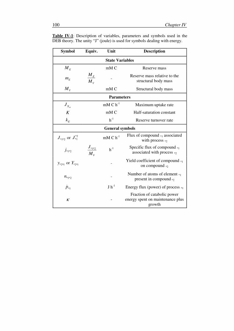
Chapter IV 100
Table IV-1: Description of variables, parameters and symbols used in the
DEB theory. The unity “J” (joule) is used for symbols dealing with energy.
Symbol Equiv. Unit Description
State Variables
EM mM C Reserve mass
Em
E
V
M
M -
Reserve mass relative to the
structural body mass
VM mM C Structural body mass
Parameters
mXJ mM C h
-1 Maximum uptake rate
K mM C Half-saturation constant
Ek h
-1 Reserve turnover rate
General symbols
*1*2J or *2*1J
mM C h
-1
Flux of compound *1 associated
with process *2
*1*2j *1*2
V
J
M h
-1
Specific flux of compound *1
associated with process *2
*2*1y or *2*1Y
- Yield coefficient of compound *1
on compound *2
*1*2n
- Number of atoms of element *1
present in compound *2
*1p� J h-1
Energy flux (power) of process *1
κ
-
Fraction of catabolic power
energy spent on maintenance plus
growth
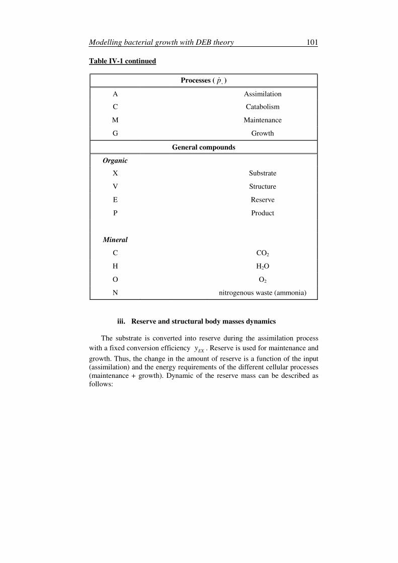
Modelling bacterial growth with DEB theory 101
Table IV-1 continued
Processes (*
p� )
A Assimilation
C Catabolism
M Maintenance
G Growth
General compounds
Organic
X Substrate
V Structure
E Reserve
P Product
Mineral
C CO2
H H2O
O O2
N nitrogenous waste (ammonia)
iii. Reserve and structural body masses dynamics
The substrate is converted into reserve during the assimilation process
with a fixed conversion efficiency EX
y . Reserve is used for maintenance and
growth. Thus, the change in the amount of reserve is a function of the input
(assimilation) and the energy requirements of the different cellular processes
(maintenance + growth). Dynamic of the reserve mass can be described as
follows:
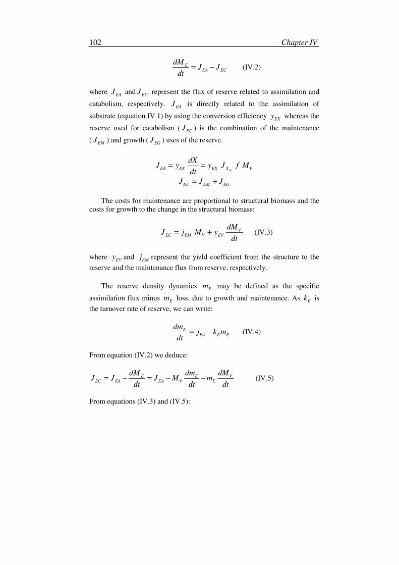
Chapter IV 102
EEA EC
dMJ J
dt= − (IV.2)
where EA
J andEC
J represent the flux of reserve related to assimilation and
catabolism, respectively. EA
J is directly related to the assimilation of
substrate (equation IV.1) by using the conversion efficiency EX
y whereas the
reserve used for catabolism (EC
J ) is the combination of the maintenance
(EM
J ) and growth (EG
J ) uses of the reserve.
mEA EX EX X V
dXJ y y J f M
dt= =
EC EM EGJ J J= +
The costs for maintenance are proportional to structural biomass and the
costs for growth to the change in the structural biomass:
VEC EM V EV
dMJ j M y
dt= + (IV.3)
where EV
y and EM
j represent the yield coefficient from the structure to the
reserve and the maintenance flux from reserve, respectively.
The reserve density dynamics E
m may be defined as the specific
assimilation flux minus E
m loss, due to growth and maintenance. As E
k is
the turnover rate of reserve, we can write:
EEA E E
dmj k m
dt= − (IV.4)
From equation (IV.2) we deduce:
VE EEC EA EA V E
dMdM dmJ J J M m
dt dt dt= − = − − (IV.5)
From equations (IV.3) and (IV.5):
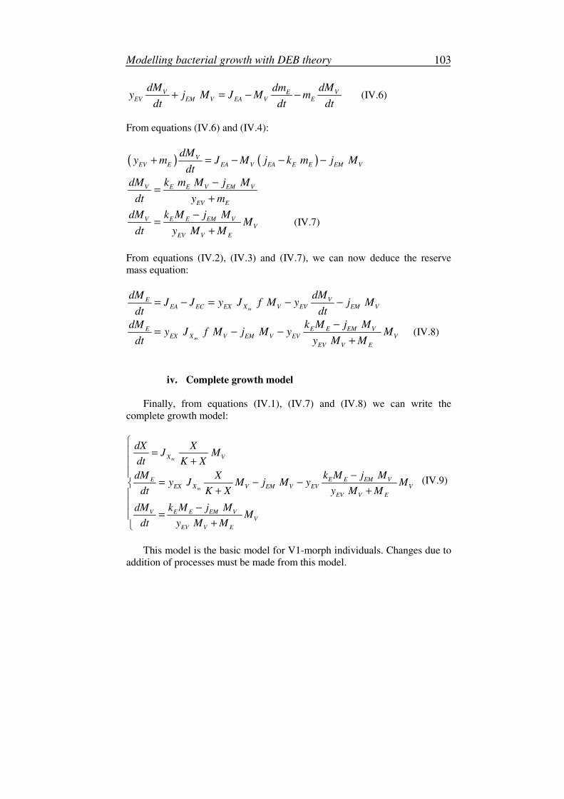
Modelling bacterial growth with DEB theory 103
V VEEV EM V EA V E
dM dMdmy j M J M m
dt dt dt+ = − − (IV.6)
From equations (IV.6) and (IV.4):
( ) ( )V
EV E EA V EA E E EM V
dMy m J M j k m j M
dt+ = − − −
V E E V EM V
EV E
dM k m M j M
dt y m
−=
+
V E E EM VV
EV V E
dM k M j MM
dt y M M
−=
+
(IV.7)
From equations (IV.2), (IV.3) and (IV.7), we can now deduce the reserve
mass equation:
m
VEEA EC EX X V EV EM V
dMdMJ J y J f M y j M
dt dt= − = − −
m
E E EM VEEX X V EM V EV V
EV V E
k M j MdMy J f M j M y M
dt y M M
−= − −
+
(IV.8)
iv. Complete growth model
Finally, from equations (IV.1), (IV.7) and (IV.8) we can write the
complete growth model:
m
m
X V
E E EM VEEX X V EM V EV V
EV V E
V E E EM VV
EV V E
dX XJ M
dt K X
k M j MdM Xy J M j M y M
dt K X y M M
dM k M j MM
dt y M M
=
+ −
= − −+ +
−=
+
(IV.9)
This model is the basic model for V1-morph individuals. Changes due to
addition of processes must be made from this model.
Chapter IV 104
II. Mechanistic model simplification for
implementation in biogeochemical models: case of
bacterial DOC degradation in a variable system
Eichinger M, Kooijman SALM, Sempéré R and Poggiale JC
Submitted to Ecological Modelling
1. Introduction
The dissolved organic carbon (DOC) is recognized as the largest pool of
reduced carbon on the planet (Hedges 1992, Carlson & Ducklow 1995). This
DOC is almost exclusively consumed by bacteria in the water column, and is
thus either transformed in CO2 or transferred to higher trophic level. Recent
studies have indicated that a better understanding of organic matter (OM)
dynamics, thus of DOC dynamics, in models requires an appropriate
knowledge of bacterial dynamics (Talin et al. 2003). However, despite their
ecological role, bacteria are rarely or poorly represented (Arhonditsis & Brett
2004). Most biogeochemical models use the Monod model (Monod 1942),
that is Michaelis-Menten kinetics (Michaelis & Menten 1913), to describe
bacterial growth (Baretta-Bekker et al. 1995, Blackburn et al. 1996, Anderson
& Williams 1998, 1999, Lancelot et al. 2002, Raick et al. 2005). Later
extensions included maintenance process (known as the Marr-Pirt model)
(Marr et al. 1963, Pirt 1965) as a kind of death rate (but forming different
products).
However, some studies have demonstrated that the Monod or Marr-Pirt
models are too simplistic and that the addition of a reserve compartment as
well as a maintenance term is necessary (1) to fit bacterial dynamics in a food
chain (Kooi & Kooijman 1994) and (2) to obtain the area of bacterial
depletion, as function of the C:P and C:N ratio in chemostat and batch
experiments (Martinussen & Thingstad 1987). Indeed, this reserve
compartment and the maintenance term may play crucial roles in bacterial
dynamics as the first one acts as a buffer and allows bacteria to survive
during depletion period and the second one represents the energetic cost for a
cell to survive. The dynamic energy budget (DEB) theory (Kooijman 2000)
accounts for these two processes. This theory has been widely tested against
experimental data and used to construct numerous models for bacterial
dynamics, e.g. trophic chains in a chemostat (Kooi & Kooijman 1994),
biodegradation of multiple substrates (Brandt et al. 2003), adaptation to
changing substrate availability (Brandt et al. 2004) and application of mass
energy conservation laws (Kooijman et al. 1999).
Modelling bacterial growth with DEB theory 105
Nowadays, two major currents concerning modelling studies are in
expansion: the development of mechanistic models that account for more and
more realistic processes, as stated previously, and the improvement of
ecosystem models which is possible due to the progress in modern computing
power and the advances in ecosystem and ecological theory (Fulton et al.
2004, Raick et al. 2006). Developing mechanistic models is a major
challenge in oceanography as it allows improving our understanding of how
the marine organisms respond to direct or indirect environmental or anthropic
perturbations. However, the inclusion of complex formulations in
biogeochemical models often leads to model that are inexorably too large,
difficult to parameterise and to deal with (Raick et al. 2006). A long pattern
of studies try to estimate the effect of physiological details on model
performance (Murray & Parslow 1999, Fulton et al. 2004, Raick et al. 2006,
Lawrie & Hearne 2007). The methods used to investigate the impact of
complexity on model performance are various: some authors compare several
levels of sophistication in the model formulation and compare their
performance to observations (Fulton et al. 2004, Baklouti et al. 2006b, Raick
et al. 2006) or compare the qualitative dynamics of two levels of models
(Murray & Parslow 1999, Baird et al. 2003, Guven & Howard 2007). These
studies generally lead to the conclusion that simpler models do capture the
crucial dynamics of the complex models. However, to construct a
mechanistic model and testing its performance towards reduced models, we
need biological information (Flynn 2005). The relevant physiological
processes are poorly known (Baird et al. 2003) and the results of experiments
carried out on bacterial populations are typically too scattery to allow the
application of complex models.
Models describing bacterial dynamics are often based on biodegradation
experiments with batch cultures, i.e. with a certain quantity of substrate and
of bacteria in the beginning of the experiment and where the system evolves
without any modification during the time course of the experiment (Zweifel
et al. 1993, Carlson & Ducklow 1996, Sempéré et al. 2000, Carlson et al.
2002, Sempéré et al. 2003, Cherrier & Bauer 2004, Eichinger et al. 2006).
The Monod model is typically used to fit data from batch experiments and
also to describe bacteria-substrate interactions in biogeochemical models.
The chemical composition in ecosystems can differ substantially for that used
in the batch cultures, which can affect the biodegradation process. Another
weakness of this scale transfer from laboratory to the ecosystem environment
is that the local environment in the ecosystem is typically much more
dynamic. Organisms are continuously subjected to perturbations and the
bacterial carbon demand is fuelled by episodic input of dissolved OM.
Indeed, food is not continuously available in natural environment (Hanegraaf
Chapter IV 106
& Kooi 2002), contrary to the batch experiments generally carried out to
determine parameters as the bacterial growth efficiency (del Giorgio & Cole
1998). Long periods of absence of one or more nutrients (Konopka 1999)
alternate with short periods of high substrate availability. The transient
behaviour of DOC is very dynamic: the DOC concentration (1) shifts during
a phytoplankton bloom (Miki & Yamamura 2005b), (2) varies greatly due to
the DOC release by phytoplankton (Grossart & Simon 2007), fluctuates (3)
seasonally, as well as non-periodically, as temporal input due to the rain
(Miki & Yamamura 2005a), or (4) cyclically as a result of the hydrological
effects in floodplains, like in Amazonian ecosystems (Farjalla et al. 2006) or
in the Okavango Delta of Botswana (Mladenov et al. 2005, Mladenov et al.
2007), (5) changes by upwelling events (Mcmanus & Peterson 1988). This
episodic character of the DOC as substrate for heterotrophic bacteria has thus
to be considered in the experiments as well as in the models.
Here we describe in the first section an experiment that has specifically
been set up to mimic the availability of substrate under field conditions.
Then, we specify a mechanistic model, constructed from the DEB theory
(Kooijman 2000) and taking into account the reserve and the maintenance
processes, as these latter processes seem necessary when dealing with
variable environment. In the next section we simplify it for implementation in
biogeochemical models. The mechanistic model and its simplification are
dynamically compared in the fourth section. The results are discussed in a
wider modelling context in the last section.
2. Description of the experiments
The carbon substrate pyruvate was periodically added during 10 days to a
batch culture of the bacterial strain Alteromonas infernus. Since other
nutrients are in excess, the fed-bacth culture was carbon-limited with
pyruvate as the only carbon source. The culture was incubated in a temperate
room in the dark at 25 ± 1°C and gently swirled. The initial carbon substrate
concentration [C(0)] was about 1.6 C mM C, whereas substrate pulses of
[C(0)] concentration were added every 48 hours. This pulse period was
chosen so that bacteria were starved between two pulses, allowing the study
of the cell maintenance and the relevance of a reserve compartment. The
experiment lasted approximately 230 hours, so there were 5 pulses, including
the initial pulse at time zero. The measured variables are DOC, which
includes the substrate and all other DOC forms that may be produced during
the time course of the experiment, and particulate organic carbon (POC),
which corresponds to the bacterial biomass-carbon. The reproducibility of the
results of this experiment was demonstrated (Eichinger et al., unpublished
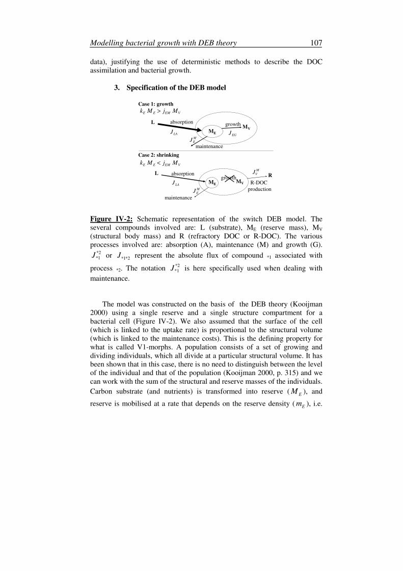
Modelling bacterial growth with DEB theory 107
data), justifying the use of deterministic methods to describe the DOC
assimilation and bacterial growth.
3. Specification of the DEB model
ME
MV
L
Case 1: growth
absorption growth
maintenance
MEMV
L
Case 2: shrinking
absorptiongrowth
maintenance
R
LAJEGJ
M
EJ
R-DOC
productionM
EJ
E E EM Vk M j M>
E E EM Vk M j M<
M
VJ
LAJ
Figure IV-2: Schematic representation of the switch DEB model. The
several compounds involved are: L (substrate), ME (reserve mass), MV
(structural body mass) and R (refractory DOC or R-DOC). The various
processes involved are: absorption (A), maintenance (M) and growth (G). *2*1J or *1*2J represent the absolute flux of compound *1 associated with
process *2. The notation *2*1J is here specifically used when dealing with
maintenance.
The model was constructed on the basis of the DEB theory (Kooijman
2000) using a single reserve and a single structure compartment for a
bacterial cell (Figure IV-2). We also assumed that the surface of the cell
(which is linked to the uptake rate) is proportional to the structural volume
(which is linked to the maintenance costs). This is the defining property for
what is called V1-morphs. A population consists of a set of growing and
dividing individuals, which all divide at a particular structural volume. It has
been shown that in this case, there is no need to distinguish between the level
of the individual and that of the population (Kooijman 2000, p. 315) and we
can work with the sum of the structural and reserve masses of the individuals.
Carbon substrate (and nutrients) is transformed into reserve (E
M ), and
reserve is mobilised at a rate that depends on the reserve density (E
m ), i.e.
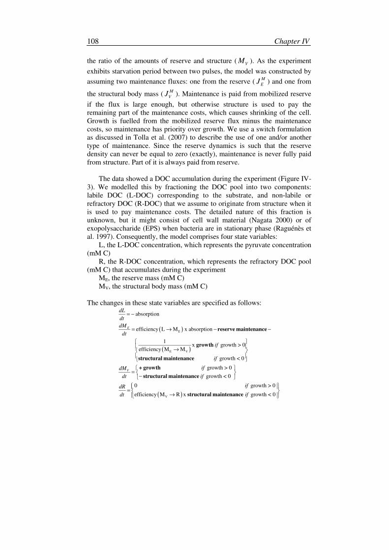
Chapter IV 108
the ratio of the amounts of reserve and structure (V
M ). As the experiment
exhibits starvation period between two pulses, the model was constructed by
assuming two maintenance fluxes: one from the reserve (M
EJ ) and one from
the structural body mass (M
VJ ). Maintenance is paid from mobilized reserve
if the flux is large enough, but otherwise structure is used to pay the
remaining part of the maintenance costs, which causes shrinking of the cell.
Growth is fuelled from the mobilized reserve flux minus the maintenance
costs, so maintenance has priority over growth. We use a switch formulation
as discussed in Tolla et al. (2007) to describe the use of one and/or another
type of maintenance. Since the reserve dynamics is such that the reserve
density can never be equal to zero (exactly), maintenance is never fully paid
from structure. Part of it is always paid from reserve.
The data showed a DOC accumulation during the experiment (Figure IV-
3). We modelled this by fractioning the DOC pool into two components:
labile DOC (L-DOC) corresponding to the substrate, and non-labile or
refractory DOC (R-DOC) that we assume to originate from structure when it
is used to pay maintenance costs. The detailed nature of this fraction is
unknown, but it might consist of cell wall material (Nagata 2000) or of
exopolysaccharide (EPS) when bacteria are in stationary phase (Raguénès et
al. 1997). Consequently, the model comprises four state variables:
L, the L-DOC concentration, which represents the pyruvate concentration
(mM C)
R, the R-DOC concentration, which represents the refractory DOC pool
(mM C) that accumulates during the experiment
ME, the reserve mass (mM C)
MV, the structural body mass (mM C)
The changes in these state variables are specified as follows:
( )
( )
E
E V
absorption
efficiency L M x absorption
1x growth > 0
efficiency M M
growth < 0
growth > 0
gro
E
V
dL
dt
dM
dt
if
if
ifdM
ifdt
= −
= → − −
→
=
−
reserve maintenance
growth
structural maintenance
+ growth
structural maintenance
( )V
wth < 0
0 growth > 0
efficiency M R x growth < 0
ifdR
ifdt
=
→ structural maintenance
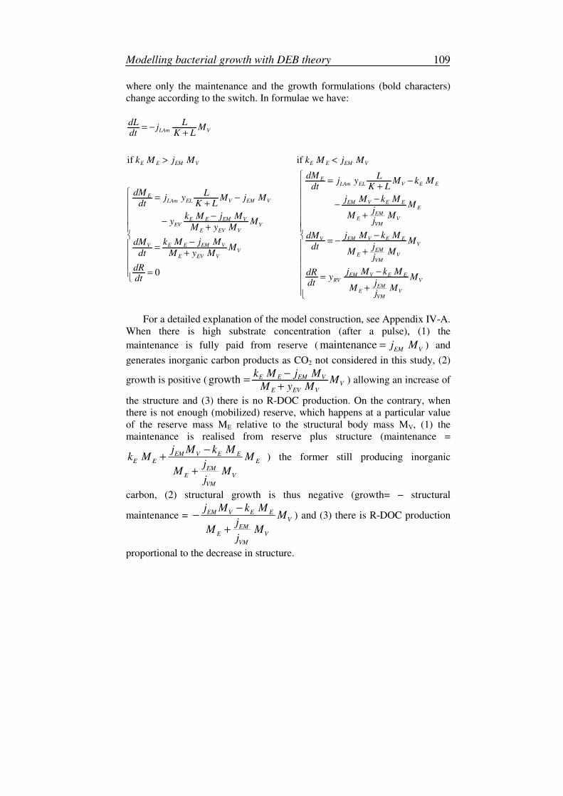
Modelling bacterial growth with DEB theory 109
where only the maintenance and the growth formulations (bold characters)
change according to the switch. In formulae we have:
if if
0
LAm V
E E EM V E E EM V
ELAm EL V E E
ELAm EL V EM V EM V E E
EEM
E VE E EM VVMEV V
E EV V
EM V E EV
E E EM VVV
E EV V
dL Lj M
dt K L
k M j M k M j M
dM Lj y M k M
dt K LdM L
j y M j M j M k Mdt K L M
jM Mk M j M
jy MM y M
j M k MdMk M j MdM
dtMdt M y M
dRdt
= −+
> <
= −+
= − − + −
+−
−+
−= −− =
+
=
VEM
E VVM
EM V E ERV V
EME V
VM
Mj
M Mj
j M k MdRy M
dt jM M
j
+
−=
+
For a detailed explanation of the model construction, see Appendix IV-A.
When there is high substrate concentration (after a pulse), (1) the
maintenance is fully paid from reserve ( maintenanceEM V
j M= ) and
generates inorganic carbon products as CO2 not considered in this study, (2)
growth is positive ( growth E E EM VV
E EV V
k M j MM
M y M
−=
+) allowing an increase of
the structure and (3) there is no R-DOC production. On the contrary, when
there is not enough (mobilized) reserve, which happens at a particular value
of the reserve mass ME relative to the structural body mass MV, (1) the
maintenance is realised from reserve plus structure (maintenance =
EM V E EE E E
EME V
VM
j M k Mk M M
jM M
j
−+
+
) the former still producing inorganic
carbon, (2) structural growth is thus negative (growth= − structural
maintenance = EM V E EV
EME V
VM
j M k MM
jM M
j
−−
+
) and (3) there is R-DOC production
proportional to the decrease in structure.
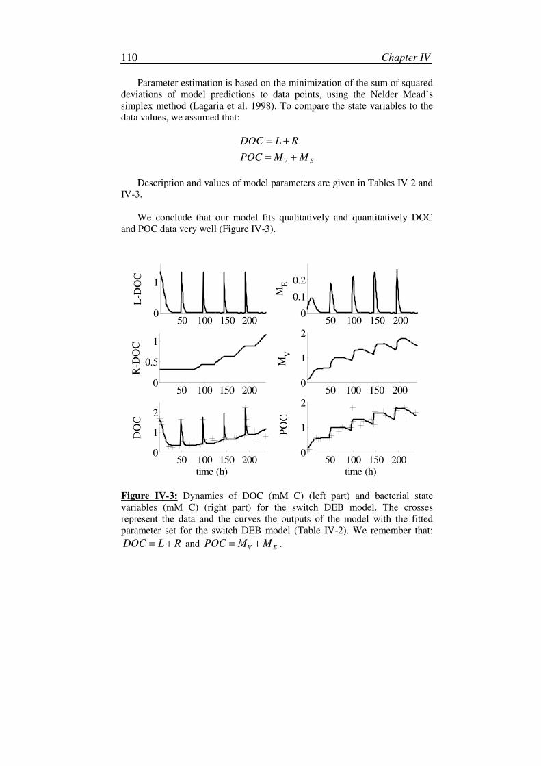
Chapter IV 110
Parameter estimation is based on the minimization of the sum of squared
deviations of model predictions to data points, using the Nelder Mead’s
simplex method (Lagaria et al. 1998). To compare the state variables to the
data values, we assumed that:
V E
DOC L R
POC M M
= +
= +
Description and values of model parameters are given in Tables IV 2 and
IV-3.
We conclude that our model fits qualitatively and quantitatively DOC
and POC data very well (Figure IV-3).
50 100 150 2000
1
L-D
OC
50 100 150 2000
0.5
1
R-D
OC
50 100 150 2000
1
2
time (h)
DO
C
50 100 150 2000
0.1
0.2M
E
50 100 150 2000
1
2
MV
50 100 150 2000
1
2
time (h)
PO
C
Figure IV-3: Dynamics of DOC (mM C) (left part) and bacterial state
variables (mM C) (right part) for the switch DEB model. The crosses
represent the data and the curves the outputs of the model with the fitted
parameter set for the switch DEB model (Table IV-2). We remember that:
DOC L R= + and V EPOC M M= + .
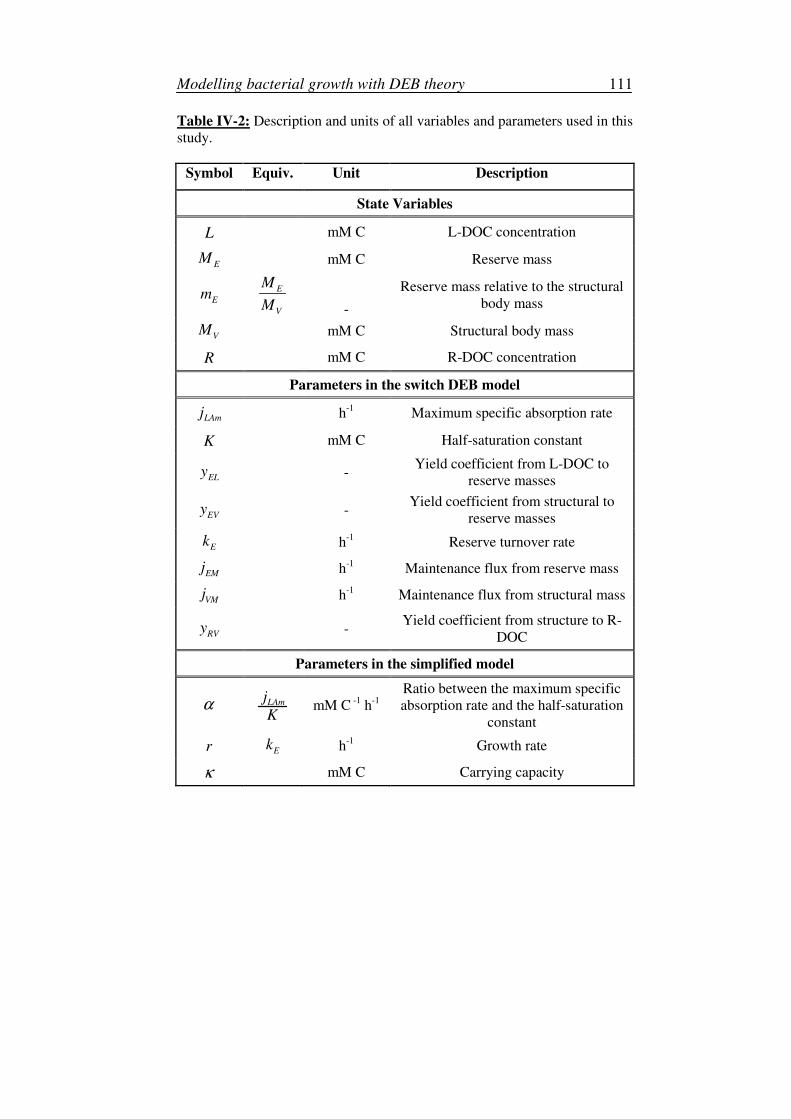
Modelling bacterial growth with DEB theory 111
Table IV-2: Description and units of all variables and parameters used in this
study.
Symbol Equiv. Unit Description
State Variables
L mM C L-DOC concentration
EM mM C Reserve mass
Em
E
V
M
M
-
Reserve mass relative to the structural
body mass
VM mM C Structural body mass
R mM C R-DOC concentration
Parameters in the switch DEB model
LAmj h-1
Maximum specific absorption rate
K mM C Half-saturation constant
ELy -
Yield coefficient from L-DOC to
reserve masses
EVy -
Yield coefficient from structural to
reserve masses
Ek h
-1 Reserve turnover rate
EMj h
-1 Maintenance flux from reserve mass
VMj h
-1 Maintenance flux from structural mass
RVy
-
Yield coefficient from structure to R-
DOC
Parameters in the simplified model
α LAmj
K mM C
-1 h
-1
Ratio between the maximum specific
absorption rate and the half-saturation
constant
r Ek h
-1 Growth rate
κ mM C Carrying capacity
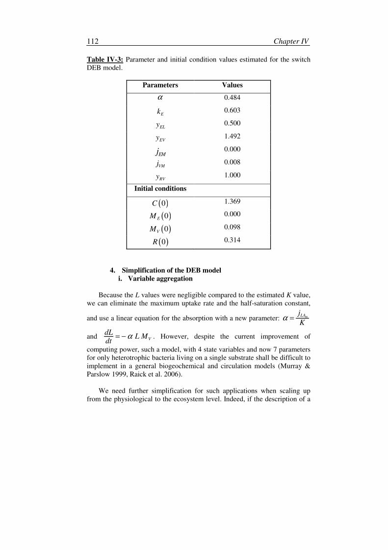
Chapter IV 112
Table IV-3: Parameter and initial condition values estimated for the switch
DEB model.
Parameters Values
α 0.484
Ek 0.603
ELy 0.500
EVy 1.492
EMj 0.000
VMj 0.008
RVy 1.000
Initial conditions
( )0C 1.369
( )0EM 0.000
( )0VM 0.098
( )0R 0.314
4. Simplification of the DEB model
i. Variable aggregation
Because the L values were negligible compared to the estimated K value,
we can eliminate the maximum uptake rate and the half-saturation constant,
and use a linear equation for the absorption with a new parameter: mLAj
Kα =
and V
dLL M
dtα= − . However, despite the current improvement of
computing power, such a model, with 4 state variables and now 7 parameters
for only heterotrophic bacteria living on a single substrate shall be difficult to
implement in a general biogeochemical and circulation models (Murray &
Parslow 1999, Raick et al. 2006).
We need further simplification for such applications when scaling up
from the physiological to the ecosystem level. Indeed, if the description of a
Modelling bacterial growth with DEB theory 113
given process at the physiological level generally requires a fine scale of
observation that subsequently generates intricate formulations, the resulting
model can ultimately be simplified and adapted to a larger scale of
observation (Baklouti et al. 2006a). Several methods exist to reduce a model,
as statistical approaches or aggregation of state variables, where some
processes are reformulated, short-circuited or not represented (Iwasa et al.
1989, Raick et al. 2006). Lots of studies use the aggregation of variables, but
they often do that in a theoretical way without any data support, for example
by using a static instead of a dynamical model when working on large time
scale (Baklouti et al. 2006b) or by aggregating the physiological processes
into less equations (Fulton et al. 2004).
In this study, the model was simplified by considering the mass balance
on model equations and by applying the perturbation theory (Appenix IV-B).
According to the reserve mass value to the structural mass value (switch
value), we have considered several mass balances. In the first case (when
growth is positive), 1T
C is the total C-mass in the system and is expressed as
a weighted sum of the three state variables L , E
M and V
M (as derivative of
R is null in this case). Using the perturbation theory, it results that 1T
C is not
constant but varies as a function of time. E
M can now be expressed as a
weighted sum of 1T
C and the two other state variables L and V
M . We also
demonstrated that V
M can be described by a logistic-like function, where the
growth rate ( r ) equals the reserve turnover rate of the DEB model (E
k ) and
the carrying capacity 1κ is a function of L and 1T
C . In the second case
(when growth is negative), mass balance is fractionated into two parts: 2T
C is
a weighted sum of L and E
M , 3T
C of V
M and R . 3T
C is always constant,
thus R can be expressed as a function of 3T
C and V
M . Using again the
perturbation theory, we demonstrated that 2T
C is also constant. Thus E
M
dynamic can be easily expressed as a function of 2T
C and L . The equation of
VM could also be reduced to a logistic-like growth where the growth rate
still equals the reserve turnover rate of the DEB model (E
k ) but where the
carrying capacity 2κ is a function of L and V
M , which complicates the
expression. Consequently, the complete DEB model with four state variables
reduces to a system of two differential equations (derivatives of L and V
M ),
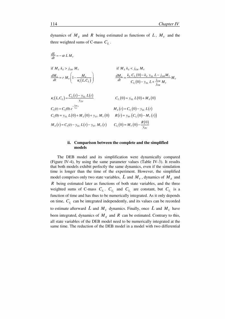
Chapter IV 114
dynamics of E
M and R being estimated as functions of L , V
M and the
three weighted sums of C-mass *T
C .
( )
( )
( )
( )( ) ( )
( ) ( ) ( )
( ) ( ) ( )
( ) ( )
2
12
1
1 2
1 1 2
1
1
1
if if
01
, 0
, 0 0 0
( ) (0) 0
(0) 0 0
EM
EV
V
E E EM V E E EM V
E T E EL EM VV V VV V
EMTT EL V
VM
T EL
T T EL EEV
jt
yT T E T EL
T EL E EV V
dLL M
dt
M k j M M k j M
k C k y L j MdM M dMr M M
dt dt jL C C y L Mj
C t y L tL C C y L M
y
C t C e M t C y L t
C y L M y M
α
κ
κ
−
= −
> <
− −
= − = − +
−
= = +
= = −
= + + ( ) ( ) ( ) ( )( )
( ) ( ) ( ) ( ) ( )( )
3
1 3
0 0
0( ) 0 0
RV T V
E T EL EV V T VRV
R t y C M t
RM t C t y L t y M t C M
y
= −
= − − = −
ii. Comparison between the complete and the simplified
models
The DEB model and its simplification were dynamically compared
(Figure IV-4), by using the same parameter values (Table IV-3). It results
that both models exhibit perfectly the same dynamics, even if the simulation
time is longer than the time of the experiment. However, the simplified
model comprises only two state variables, L and V
M , dynamics of E
M and
R being estimated later as functions of both state variables, and the three
weighted sums of C-mass *T
C . 2T
C and 3T
C are constant, but 1T
C is a
function of time and has thus to be numerically integrated. As it only depends
on time, 1T
C can be integrated independently, and its values can be recorded
to estimate afterward L and V
M dynamics. Finally, once L and V
M have
been integrated, dynamics of E
M and R can be estimated. Contrary to this,
all state variables of the DEB model need to be numerically integrated at the
same time. The reduction of the DEB model in a model with two differential
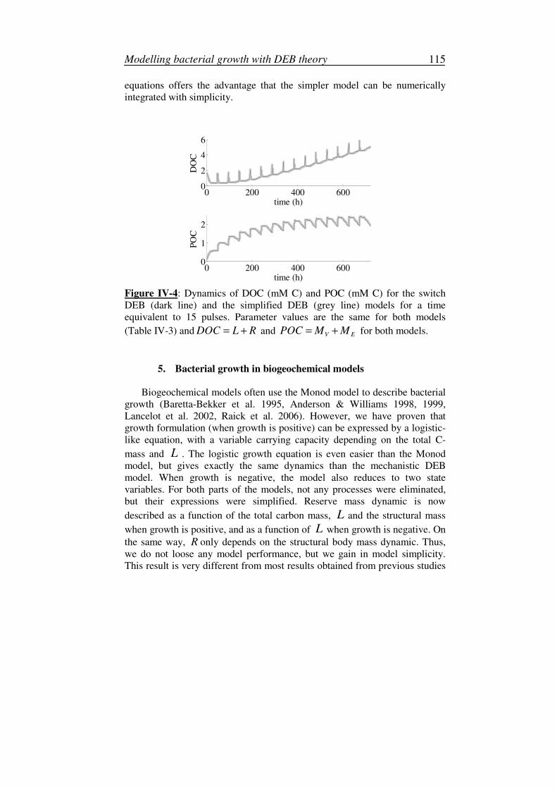
Modelling bacterial growth with DEB theory 115
equations offers the advantage that the simpler model can be numerically
integrated with simplicity.
0 200 400 6000
2
4
6
time (h)D
OC
0 200 400 6000
1
2
time (h)
PO
C
Figure IV-4: Dynamics of DOC (mM C) and POC (mM C) for the switch
DEB (dark line) and the simplified DEB (grey line) models for a time
equivalent to 15 pulses. Parameter values are the same for both models
(Table IV-3) and DOC L R= + and V EPOC M M= + for both models.
5. Bacterial growth in biogeochemical models
Biogeochemical models often use the Monod model to describe bacterial
growth (Baretta-Bekker et al. 1995, Anderson & Williams 1998, 1999,
Lancelot et al. 2002, Raick et al. 2006). However, we have proven that
growth formulation (when growth is positive) can be expressed by a logistic-
like equation, with a variable carrying capacity depending on the total C-
mass and L . The logistic growth equation is even easier than the Monod
model, but gives exactly the same dynamics than the mechanistic DEB
model. When growth is negative, the model also reduces to two state
variables. For both parts of the models, not any processes were eliminated,
but their expressions were simplified. Reserve mass dynamic is now
described as a function of the total carbon mass, L and the structural mass
when growth is positive, and as a function of L when growth is negative. On
the same way, R only depends on the structural body mass dynamic. Thus,
we do not loose any model performance, but we gain in model simplicity.
This result is very different from most results obtained from previous studies
Chapter IV 116
on model reduction, as these latter studies generally search the best
compromise between model performance and complexity, but they always
loose performance to gain simplicity (Murray & Parslow 1999, Fulton et al.
2004, Baklouti et al. 2006b, Raick et al. 2006). For example, by using a
Monod or a Marr-Pirt model, which are both special cases of the DEB model
and thus simplifications of our model, we should eliminate the reserve mass
variable. DEB model simulations show that the reserve mass dynamics are
indeed faster than structural mass dynamics, and that reserve mass values are
also smaller than structural mass values (Figure IV-3). Consequently, reserve
mass dynamics could be neglected compare to other state variable dynamics.
This would effectively lead in further model simplifications. Nevertheless, it
has still been proven that bacteria are able to store carbon in carbon limited
systems (Baxter & Sieburth 1984) and in non carbon limited systems
(Kooijman 2000). If growth is limited by nutrients such as nitrate or
phosphate, the carbon reserve can become important (Kooijman and Troost,
2007). Confrontation between data and models have also demonstrated that
the addition of the reserve and the maintenance are necessary in the Monod
model to reproduce dynamics of a tri-trophic food chain including bacteria
(Kooi & Kooijman 1994, Nisbet et al. 2000). To conclude, our model
reduction doesn’t reduce model insight as it still comprises necessary
processes to describe bacterial growth. Computational costs are greatly
decreased, which is of great interest for further coupling of this bacterial
growth model with biogeochemical and hydrodynamical transport models
(Baklouti et al. 2006b). Moreover, this simplification gives a mechanistic
basis to the logistic equation considered as an empirical formulation.
6. Conclusion
The comparison of mechanistic models to their simplifications, and
moreover based on data set as in this study, allows the examination of the
effects of alternative process formulations on model behaviour (Murray &
Parslow 1999). The outcome of this kind of study takes all its importance
when we can demonstrated that a simplified model behaves and fits equally
than the complex formulation, as the simpler model uses less number of
parameters, less of development time and less time to validate, verify and
calibrate (Fulton et al. 2004). This simplification step is crucial when we aim
to implement mechanistic-growth model in global models. The coupling
between experimentation and modelling approaches is very important as it
allows model simplification on an experimental data basis, and not only on
theoretical dynamics.
Modelling bacterial growth with DEB theory 117
However, other experiments with other kinds of perturbations and
inclusion of trophic relation should be done to test the relevance of a reserve
compartment for marine bacteria. Our expectations for when reserve might
be important should be tested with experiments. The application of
mechanistic models is only feasible if the critical variables have been
measured (Flynn 2005). However, these complex models are difficult to
calibrate accurately without accurate data sets. Nevertheless, even if
physiological details are not necessarily needed for global models, such
models can still be used to identify critical variables: if a detailed model does
not match an experimental data set well, it is likely that it does miss an
essential process (Flynn 2005).
III. Implementation of the respiration in DEB models
1. Development of the O2 flux formulation
The DEB theory allows the evaluation of respiration, i.e. the use of
dioxygen. During the experiments, O2 consumption was also measured at
each point in time. We have thus decided to use this data set in a modelling
purpose. This will give a best insight of bacterial metabolism. Since energy
for the conversion of substrate into reserve is extracted from substrate,
assimilation has an anabolic as well as a catabolic aspect. Moreover, energy
for the reserve conversion into structure is extracted from reserve, thus
growth has also an anabolic and a catabolic aspect. The O2 flux was
determined from Table IV-4.
From this table we can first deduce each yield coefficient by multiplying
the line of the considered yield coefficient by the line of the considered
element C, H, O or N, the sum of this multiplication being 0 to respect the
mass balance law. For example, to determinea
OLY , we have to multiply the
line of the anabolic assimilation with the line of oxygen indices:
( )
2 1 0
1
2
a a
HL OL OE
a
OE HLa
OL
Y Y n
n YY
+ − − =
+ −
=
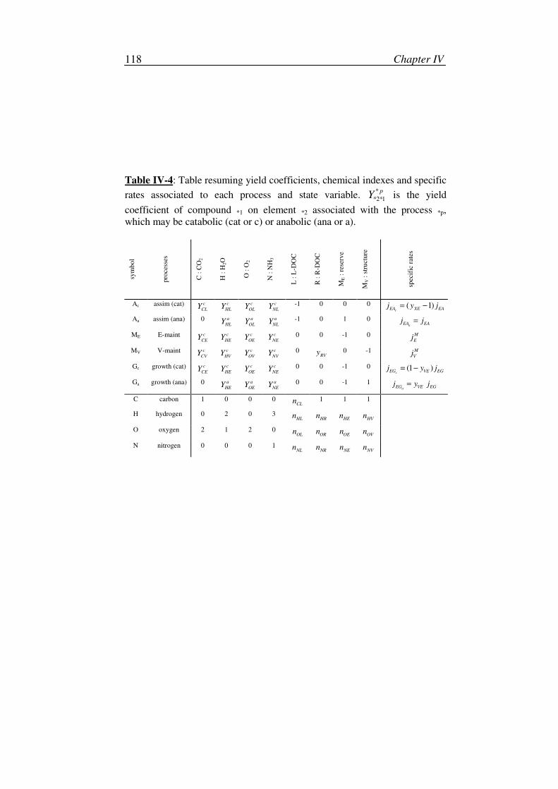
Chapter IV 118
Table IV-4: Table resuming yield coefficients, chemical indexes and specific
rates associated to each process and state variable. *
*2*1
pY is the yield
coefficient of compound *1 on element *2 associated with the process *p,
which may be catabolic (cat or c) or anabolic (ana or a).
sym
bo
l
pro
ces
ses
C :
CO
2
H :
H2O
O :
O2
N :
NH
3
L :
L-D
OC
R :
R-D
OC
ME :
res
erv
e
MV :
str
uct
ure
speci
fic r
ate
s
Ac assim (cat) c
CLY
c
HLY
c
OLY
c
NLY -1 0 0 0 ( 1)
cEA XE EAj y j= −
Aa assim (ana) 0 a
HLY a
OLY a
NLY -1 0 1 0 aEA EAj j=
ME E-maint c
CEY
c
HEY
c
OEY
c
NEY 0 0 -1 0 M
Ej
MV V-maint c
CVY
c
HVY
c
OVY
c
NVY 0
RVy 0 -1 M
Vj
Gc growth (cat) c
CEY
c
HEY
c
OEY
c
NEY 0 0 -1 0 (1 )
cEG VE EGj y j= −
Ga growth (ana) 0 a
HEY
a
OEY
a
NEY 0 0 -1 1
aEG VE EGj y j=
C carbon 1 0 0 0 CL
n 1 1 1
H hydrogen 0 2 0 3 HL
n HR
n HE
n HV
n
O oxygen 2 1 2 0 OLn
ORn OEn
OVn
N nitrogen 0 0 0 1 NL
n NR
n NE
n NV
n
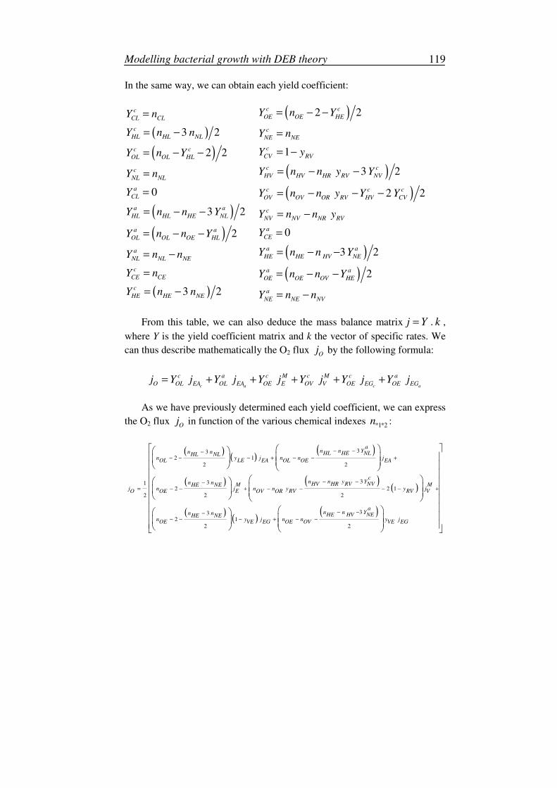
Modelling bacterial growth with DEB theory 119
In the same way, we can obtain each yield coefficient:
( )
( )
( )
( )
( )
3 2
2 2
0
3 2
2
3 2
c
CL CL
c
HL HL NL
c c
OL OL HL
c
NL NL
a
CL
a a
HL HL HE NL
a a
OL OL OE HL
a
NL NL NE
c
CE CE
c
HE HE NE
Y n
Y n n
Y n Y
Y n
Y
Y n n Y
Y n n Y
Y n n
Y n
Y n n
=
= −
= − −
=
=
= − −
= − −
= −
=
= −
( )
( )
( )
( )
( )
2 2
1
3 2
2 2
0
3 2
2
c c
OE OE HE
c
NE NE
c
CV RV
c c
HV HV HR RV NV
c c c
OV OV OR RV HV CV
c
NV NV NR RV
a
CE
a a
HE HE HV NE
a a
OE OE OV HE
a
NE NE NV
Y n Y
Y n
Y y
Y n n y Y
Y n n y Y Y
Y n n y
Y
Y n n Y
Y n n Y
Y n n
= − −
=
= −
= − −
= − − −
= −
=
= − −
= − −
= −
From this table, we can also deduce the mass balance matrix .j Y k= ,
where Y is the yield coefficient matrix and k the vector of specific rates. We
can thus describe mathematically the O2 flux O
j by the following formula:
c a c a
c a c M c M c a
O OL EA OL EA OE E OV V OE EG OE EGj Y j Y j Y j Y j Y j Y j= + + + + +
As we have previously determined each yield coefficient, we can express
the O2 flux O
j in function of the various chemical indexes *1*2n :
( )( )
( )
( ) ( )( )
( )( )
( )
332 1
2 2
3312 2 1
2 2 2
332 1
2 2
an n Yn n HL HE NLHL NL
n y j n n jLEOL EA OL OE EA
cn n y Yn n HV HR RV NVM MHE NE
j n j n n y y jE RV RV VO OE OV OR
an n Yn n HE HV NEHE NE
n y j n nVEOE EG OE OV
− −−
− − − + − − +
− −−
= − − + − − − − +
− −−
− − − + − −
y jVE EG
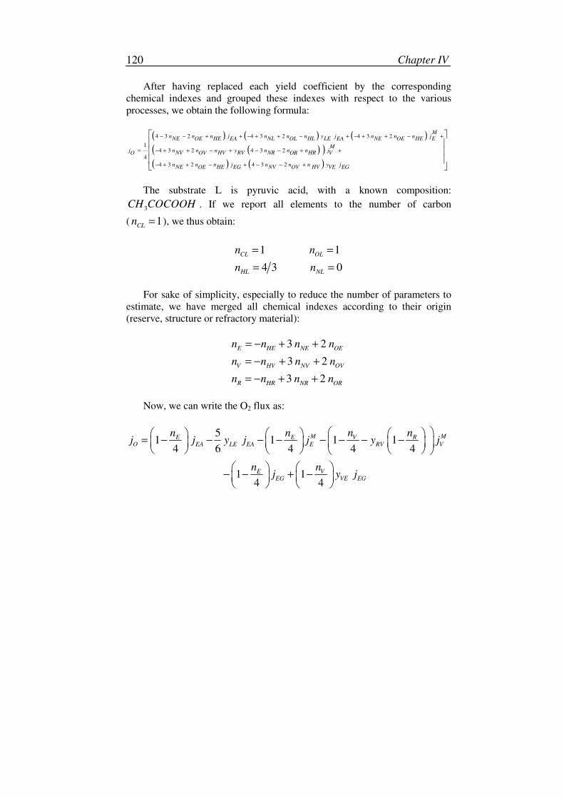
Chapter IV 120
After having replaced each yield coefficient by the corresponding
chemical indexes and grouped these indexes with respect to the various
processes, we obtain the following formula:
( ) ( ) ( )
( )( )
( ) ( )
4 3 2 4 3 2 4 3 2
14 3 2 4 3 2
4
4 3 2 4 3 2
Mn n n j n n n y j n n n jNE HE NL HL LE NE HE EOE EA OL EA OE
Mj n n n y n n n jNV HV RV NR HR VO OV OR
n n n j n n n y jNE HE NV HV VEOE EG OV EG
− − + + − + + − + − + + − +
= − + + − + − − + +
− + + − + − − +
The substrate L is pyruvic acid, with a known composition:
3CH COCOOH . If we report all elements to the number of carbon
( 1CL
n = ), we thus obtain:
1 1
4 3 0
CL OL
HL NL
n n
n n
= =
= =
For sake of simplicity, especially to reduce the number of parameters to
estimate, we have merged all chemical indexes according to their origin
(reserve, structure or refractory material):
3 2
3 2
3 2
E HE NE OE
V HV NV OV
R HR NR OR
n n n n
n n n n
n n n n
= − + +
= − + +
= − + +
Now, we can write the O2 flux as:
51 1 1 1
4 6 4 4 4
1 14 4
M MVE E RO EA LE EA E RV V
VEEG VE EG
nn n nj j y j j y j
nnj y j
= − − − − − − − −
− − + −
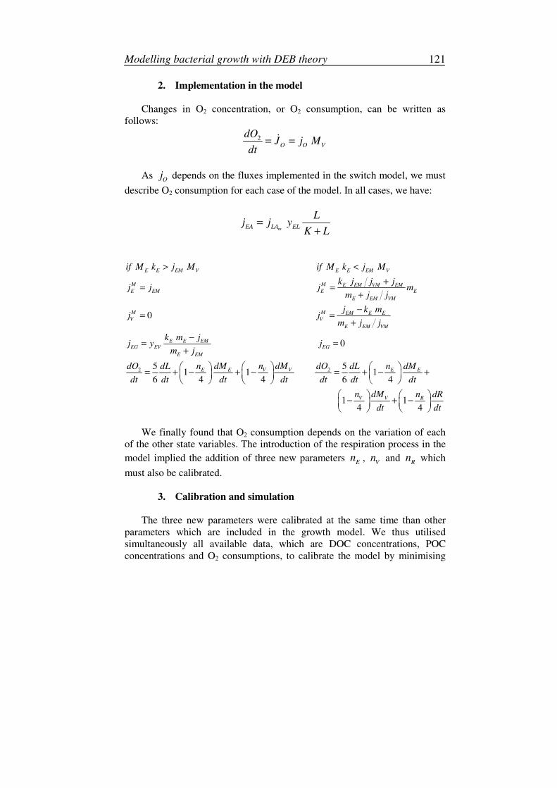
Modelling bacterial growth with DEB theory 121
2. Implementation in the model
Changes in O2 concentration, or O2 consumption, can be written as
follows:
2O O V
dOJ j M
dt= =�
As O
j depends on the fluxes implemented in the switch model, we must
describe O2 consumption for each case of the model. In all cases, we have:
mEA LA EL
Lj j y
K L=
+
2 2
0
0
5 51 1 1
6 4 4 6 4
14
E E EM V E E EM V
M M E EM VM EM
E EM E E
E EM VM
M M EM E EV V
E EM VM
E E EMEG EV EG
E EM
V VE E E E
V V
if M k j M if M k j M
k j j jj j j m
m j j
j k mj j
m j j
k m jj y j
m j
n dMdO n dM dO n dMdL dL
dt dt dt dt dt dt dt
n dM
> <
+= =
+
−= =
+
−= =
+
= + − + − = + − +
−
1
4
Rn dR
dt dt
+ −
We finally found that O2 consumption depends on the variation of each
of the other state variables. The introduction of the respiration process in the
model implied the addition of three new parameters E
n , V
n and R
n which
must also be calibrated.
3. Calibration and simulation
The three new parameters were calibrated at the same time than other
parameters which are included in the growth model. We thus utilised
simultaneously all available data, which are DOC concentrations, POC
concentrations and O2 consumptions, to calibrate the model by minimising
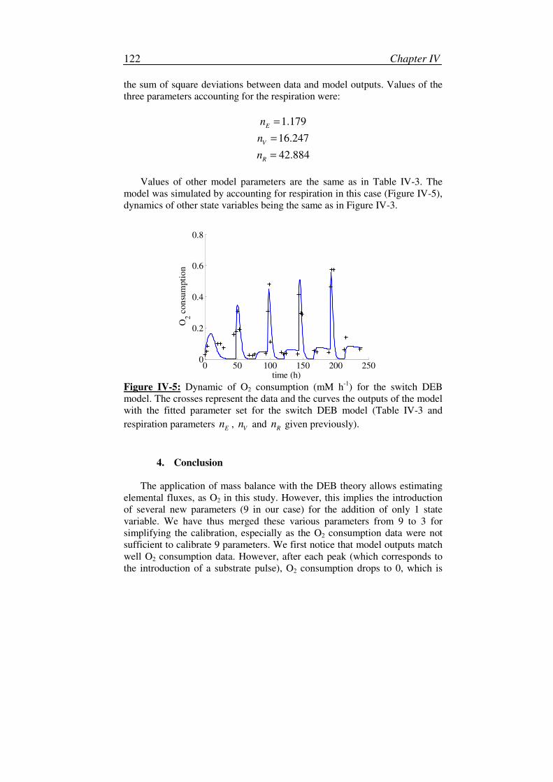
Chapter IV 122
the sum of square deviations between data and model outputs. Values of the
three parameters accounting for the respiration were:
1.179E
n =
16.247V
n =
42.884R
n =
Values of other model parameters are the same as in Table IV-3. The
model was simulated by accounting for respiration in this case (Figure IV-5),
dynamics of other state variables being the same as in Figure IV-3.
0 50 100 150 200 2500
0.2
0.4
0.6
0.8
time (h)
O2 c
on
sum
pti
on
Figure IV-5: Dynamic of O2 consumption (mM h
-1) for the switch DEB
model. The crosses represent the data and the curves the outputs of the model
with the fitted parameter set for the switch DEB model (Table IV-3 and
respiration parameters E
n , V
n and R
n given previously).
4. Conclusion
The application of mass balance with the DEB theory allows estimating
elemental fluxes, as O2 in this study. However, this implies the introduction
of several new parameters (9 in our case) for the addition of only 1 state
variable. We have thus merged these various parameters from 9 to 3 for
simplifying the calibration, especially as the O2 consumption data were not
sufficient to calibrate 9 parameters. We first notice that model outputs match
well O2 consumption data. However, after each peak (which corresponds to
the introduction of a substrate pulse), O2 consumption drops to 0, which is
Modelling bacterial growth with DEB theory 123
quite surprising. Indeed, we might assume that bacteria never stop respiration
due to maintenance, and thus consumption should not fall near zero values.
This dynamic may be due to the calibration, as it doesn’t include any
biological insight but just try to minimise the difference between model
outputs and observations. As we do not have any data which could confirm
that O2 consumption should not drop to 0, we cannot prove our assumptions.
On the other hand, our parameter values for the chemical indexes which
have allowed respiration calibration are also difficult to interpret. For
example, for the bacterial species Klebsiella aerogenes growing on glycerol,
the following parameter values were found (Hanegraaf 1997, Kooijman
2000, p 314):
1.66 0.422 0.312
1.64 0.379 0198
HE OE NE
HV OV NV
n n n
n n n
= = =
= = =
We can assume that chemical indexes are in the same order of magnitude
for organisms that can be considered equivalent on a physiological point of
view (both are heterotrophic and aerobic bacteria). This would result in our
study to parameter values that amount to:
0.120
0.288
E
V
n
n
=
= −
These values are really far from values we have estimated. However, if
O2 consumption was simulated from this parameter set, with R
n value being
a weighted sum of E
n and V
n , model outputs didn’t match data well. The
best strategy would consist in measuring these chemical indexes. But these
measurements would be highly difficult because (1) the experimental
protocol would be difficult for this kind of measurements, (2) if we
succeeded to measure these indexes for this bacterial species in culture, we
could not discriminate the composition between reserve and structure, (3) for
instance we can not separate the R-DOC from L-DOC.
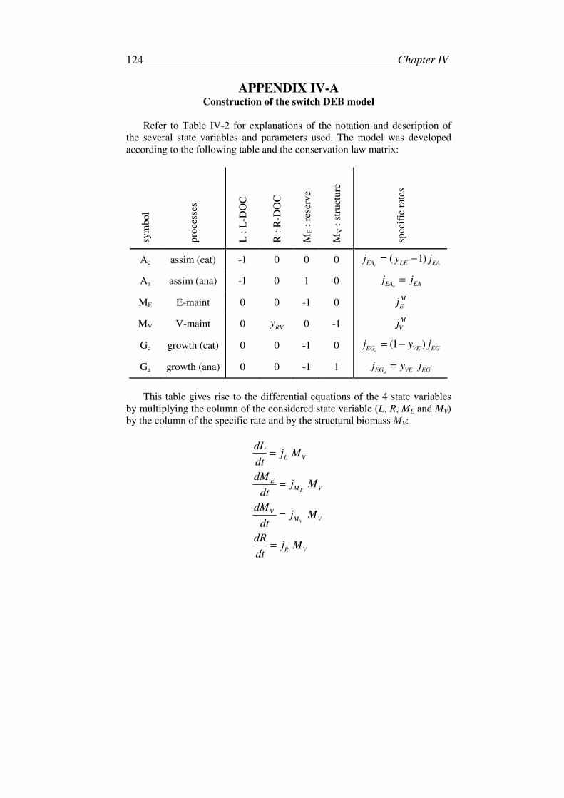
Chapter IV 124
APPENDIX IV-A Construction of the switch DEB model
Refer to Table IV-2 for explanations of the notation and description of
the several state variables and parameters used. The model was developed
according to the following table and the conservation law matrix:
sym
bo
l
pro
cess
es
L :
L-D
OC
R :
R-D
OC
ME :
res
erv
e
MV :
str
uct
ure
spec
ific
rat
es
Ac assim (cat) -1 0 0 0 ( 1)cEA LE EA
j y j= −
Aa assim (ana) -1 0 1 0 aEA EAj j=
ME E-maint 0 0 -1 0 M
Ej
MV V-maint 0 RVy 0 -1
M
Vj
Gc growth (cat) 0 0 -1 0 (1 )cEG VE EGj y j= −
Ga growth (ana) 0 0 -1 1 aEG VE EGj y j=
This table gives rise to the differential equations of the 4 state variables
by multiplying the column of the considered state variable (L, R, ME and MV)
by the column of the specific rate and by the structural biomass MV:
E
V
L V
EM V
VM V
R V
dLj M
dt
dMj M
dt
dMj M
dt
dRj M
dt
=
=
=
=
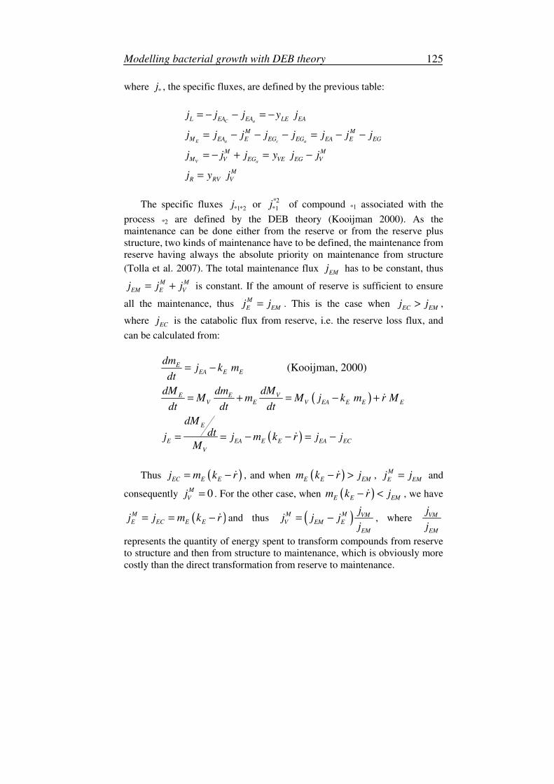
Modelling bacterial growth with DEB theory 125
where *j , the specific fluxes, are defined by the previous table:
C a
E a c a
V a
L EA EA LE EA
M M
M EA E EG EG EA E EG
M M
M V EG VE EG V
M
R RV V
j j j y j
j j j j j j j j
j j j y j j
j y j
= − − = −
= − − − = − −
= − + = −
=
The specific fluxes *1*2j or *2
*1j of compound *1 associated with the
process *2 are defined by the DEB theory (Kooijman 2000). As the
maintenance can be done either from the reserve or from the reserve plus
structure, two kinds of maintenance have to be defined, the maintenance from
reserve having always the absolute priority on maintenance from structure
(Tolla et al. 2007). The total maintenance flux EM
j has to be constant, thus
M M
EM E Vj j j= + is constant. If the amount of reserve is sufficient to ensure
all the maintenance, thus M
E EMj j= . This is the case when
EC EMj j> ,
where EC
j is the catabolic flux from reserve, i.e. the reserve loss flux, and
can be calculated from:
( )
( )
(Kooijman, 2000)EEA E E
VE EV E V EA E E E
E
E EA E E EA EC
V
dmj k m
dt
dMdM dmM m M j k m r M
dt dt dt
dMdtj j m k r j j
M
= −
= + = − +
= = − − = −
�
�
Thus ( )EC E Ej m k r= − � , and when ( )E E EMm k r j− >� , M
E EMj j= and
consequently 0M
Vj = . For the other case, when ( )E E EMm k r j− <� , we have
( )M
E EC E Ej j m k r= = − � and thus ( )M M VMV EM E
EM
jj j j
j= − , where VM
EM
j
j
represents the quantity of energy spent to transform compounds from reserve
to structure and then from structure to maintenance, which is obviously more
costly than the direct transformation from reserve to maintenance.
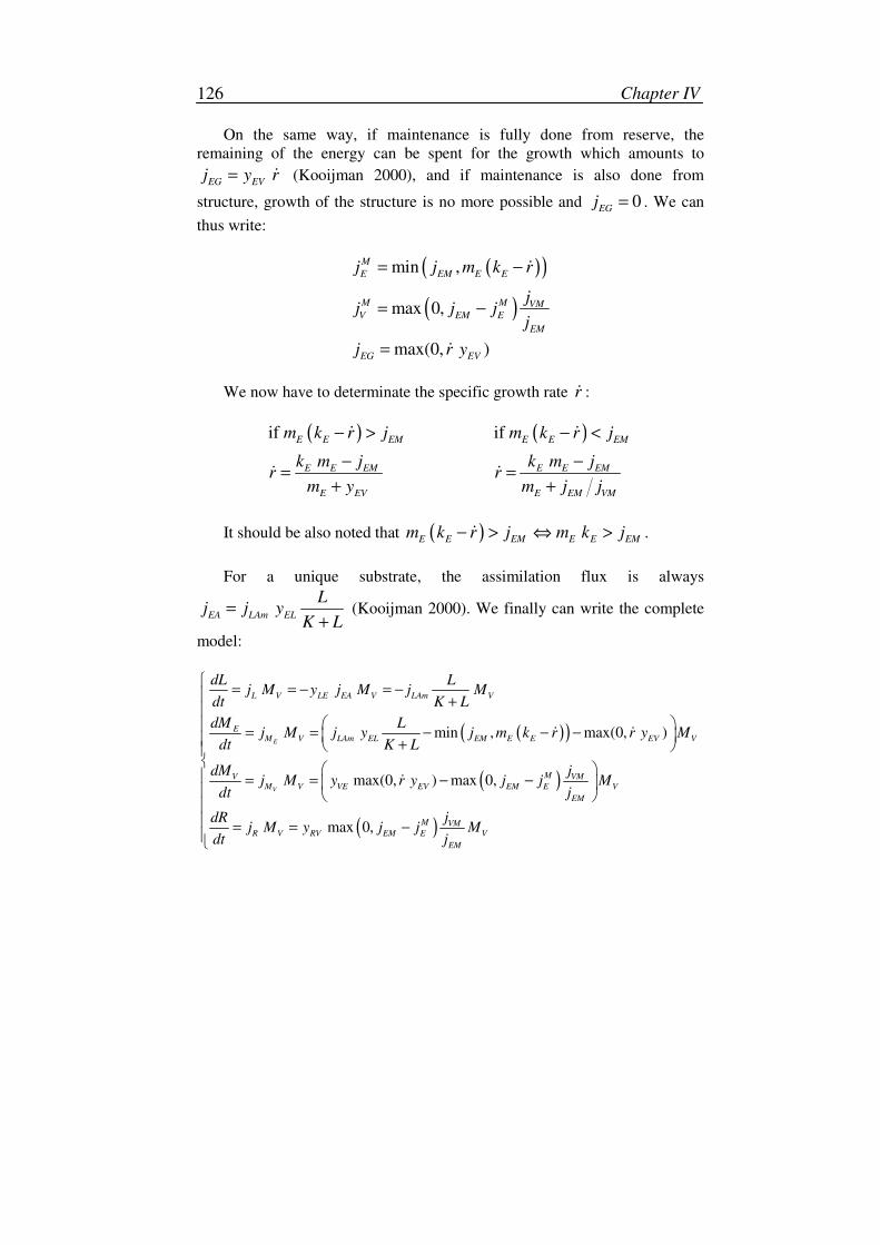
Chapter IV 126
On the same way, if maintenance is fully done from reserve, the
remaining of the energy can be spent for the growth which amounts to
EG EVj y r= � (Kooijman 2000), and if maintenance is also done from
structure, growth of the structure is no more possible and 0EG
j = . We can
thus write:
( )( )
( )
min ,
max 0,
max(0, )
M
E EM E E
M M VMV EM E
EM
EG EV
j j m k r
jj j j
j
j r y
= −
= −
=
�
�
We now have to determinate the specific growth rate r� :
( ) ( )if if E E EM E E EM
E E EM E E EM
E EV E EM VM
m k r j m k r j
k m j k m jr r
m y m j j
− > − <
− −= =
+ +
� �
� �
It should be also noted that ( )E E EM E E EMm k r j m k j− > ⇔ >� .
For a unique substrate, the assimilation flux is always
EA LAm EL
Lj j y
K L=
+
(Kooijman 2000). We finally can write the complete
model:
( )( )
( )
( )
min , max(0, )
max(0, ) max 0,
max 0,
E
V
L V LE EA V LAm V
EM V LAm EL EM E E EV V
MV VM
M V VE EV EM E V
EM
M VM
R V RV EM E V
EM
dL Lj M y j M j M
dt K L
dM Lj M j y j m k r r y M
dt K L
dM jj M y r y j j M
dt j
jdRj M y j j M
dt j
= = − = −
+
= = − − −
+ = = − −
= = −
� �
�
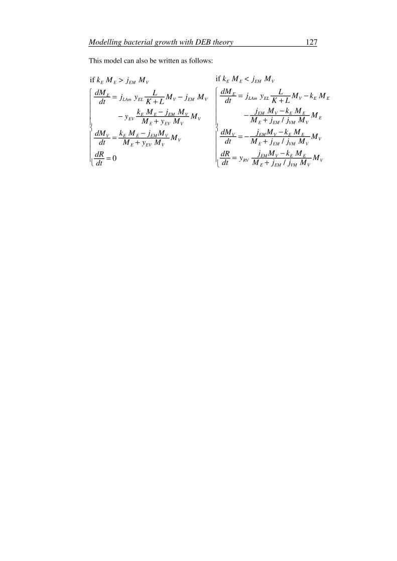
Modelling bacterial growth with DEB theory 127
This model can also be written as follows:
if if
/
/
0
E E EM VE E EM V
EELAm EL V E ELAm EL V EM V
EM V E EE E EM VEEV V
E EM VM VE EV V
EM V E EVE E EM VVVV
E EM VM VE EV V
k M j Mk M j M
dM LdM L j y M k Mj y M j Mdt K Ldt K L
j M k Mk M j M My MM j j MM y M
j M k MdMk M j MdM MMdt M j j Mdt M y M
dRdt
<>
= −= −
+ +
−−
− −++
−− = −=
++
= /
EM V E ERV V
E EM VM V
j M k MdRy M
dt M j j M
−
=+
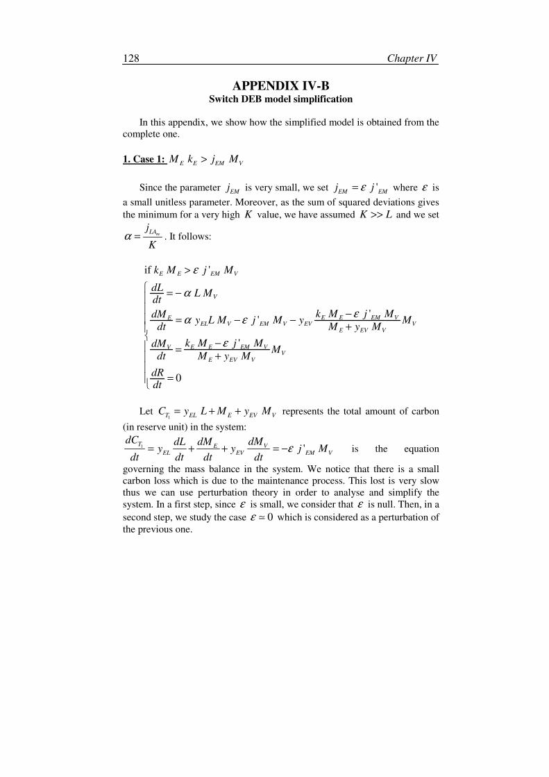
Chapter IV 128
APPENDIX IV-B Switch DEB model simplification
In this appendix, we show how the simplified model is obtained from the
complete one.
1. Case 1: E E EM V
M k j M>
Since the parameter EM
j is very small, we set 'EM EM
j jε= where ε is
a small unitless parameter. Moreover, as the sum of squared deviations gives
the minimum for a very high K value, we have assumed K L>> and we set
mLAj
Kα = . It follows:
if '
''
'
0
E E EM V
V
E E EM VEEL V EM V EV V
E EV V
E E EM VVV
E EV V
k M j M
dLL M
dt
k M j MdMy L M j M y M
dt M y M
k M j MdMM
dt M y M
dRdt
ε
α
εα ε
ε
>
= −
−= − −
+
− =+
=
Let 1T EL E EV V
C y L M y M= + + represents the total amount of carbon
(in reserve unit) in the system:
1 'T VE
EL EV EM V
dC dMdMdLy y j M
dt dt dt dtε= + + = − is the equation
governing the mass balance in the system. We notice that there is a small
carbon loss which is due to the maintenance process. This lost is very slow
thus we can use perturbation theory in order to analyse and simplify the
system. In a first step, since ε is small, we consider that ε is null. Then, in a
second step, we study the case 0ε � which is considered as a perturbation of
the previous one.
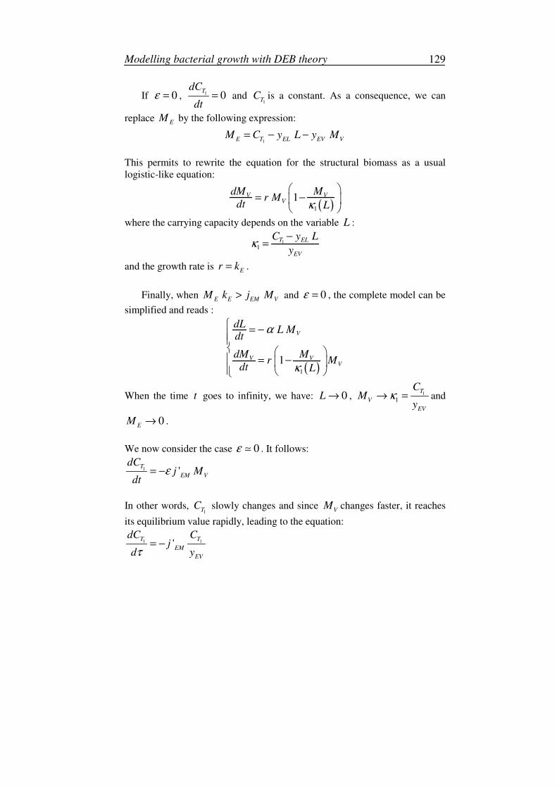
Modelling bacterial growth with DEB theory 129
If 0ε = , 1 0TdC
dt= and
1TC is a constant. As a consequence, we can
replace E
M by the following expression:
1E T EL EV VM C y L y M= − −
This permits to rewrite the equation for the structural biomass as a usual
logistic-like equation:
( )1
1V VV
dM Mr M
dt Lκ
= −
where the carrying capacity depends on the variable L :
1
1T EL
EV
C y L
yκ
−=
and the growth rate is E
r k= .
Finally, when E E EM V
M k j M> and 0ε = , the complete model can be
simplified and reads :
( )1
1
V
V VV
dLL M
dt
dM Mr M
dt L
α
κ
= −
= −
When the time t goes to infinity, we have: 0L → , 1
1
T
V
EV
CM
yκ→ = and
0E
M → .
We now consider the case 0ε � . It follows:
1 'T
EM V
dCj M
dtε= −
In other words, 1T
C slowly changes and since V
M changes faster, it reaches
its equilibrium value rapidly, leading to the equation:
1 1'T T
EM
EV
dC Cj
d yτ
= −
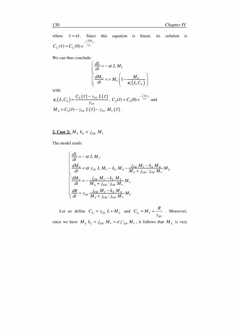
Chapter IV 130
where tτ ε= . Since this equation is linear, its solution is
1 1
'
( ) (0) EV
j EM
y
T TC C eτ
τ
−
=
We can thus conclude:
( )11
1,
V
V VV
T
dLL M
dt
dM Mr M
dt L C
α
κ
= −
= −
with:
( )( ) ( )
1
11 ,T EL
TEV
C y LL C
y
τ τκ
−
= , 1 1
'
( ) (0)EM
EV
j
yT TC C e
τ
τ
−
= and
( ) ( )1( )E T EL EV VM C y L y Mτ τ τ= − − .
2. Case 2: E E EM V
M k j M<
The model reads:
V
EM V E EEEL V E E E
E EM VM V
EM V E EVV
E EM VM V
EM V E ERV V
E EM VM V
dLL M
dt
j M k MdMy L M k M M
dt M j j M
j M k MdMM
dt M j j M
j M k MdRy M
dt M j j M
α
α
= −
−= − −
+
− = −
+ −
=+
Let us define 2T EL E
C y L M= + and 3T V
RV
RC M
y= + . Moreover,
since we have 'E E EM V EM V
M k j M j Mε< = , it follows that E
M is very
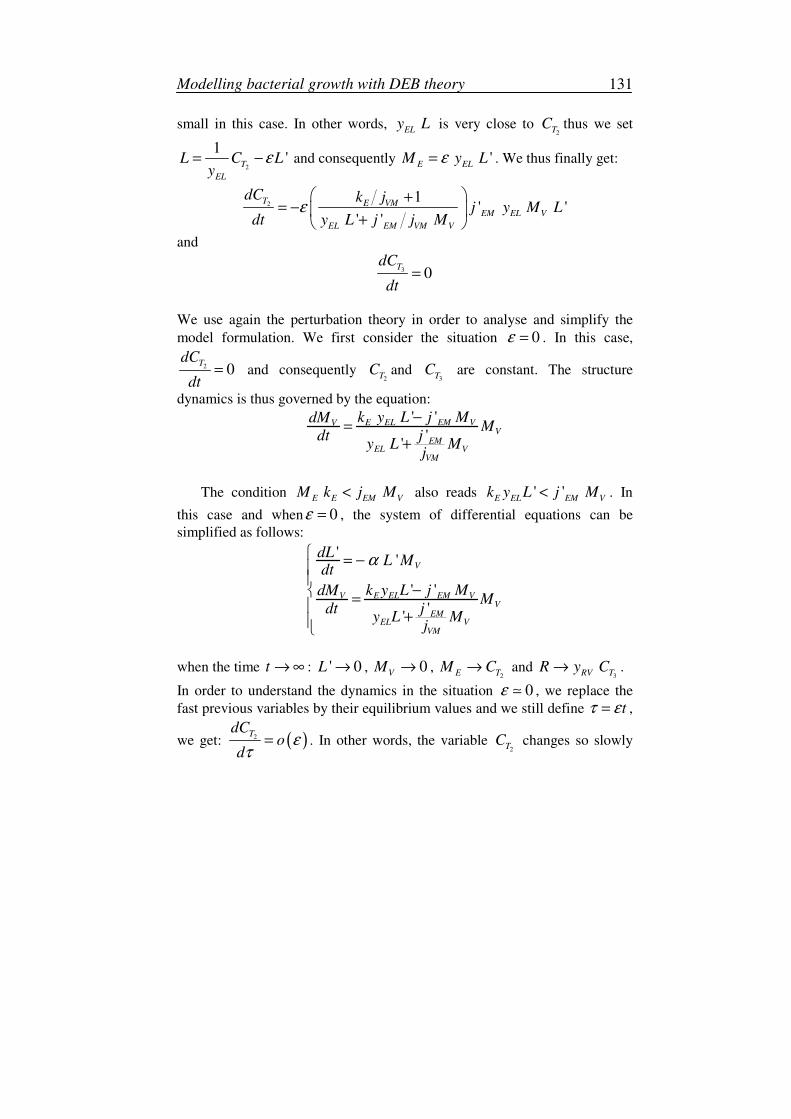
Modelling bacterial growth with DEB theory 131
small in this case. In other words, EL
y L is very close to 2T
C thus we set
2
1'
T
EL
L C Ly
ε= − and consequently 'E EL
M y Lε= . We thus finally get:
21
' '' '
T E VMEM EL V
EL EM VM V
dC k jj y M L
dt y L j j Mε
+= −
+
and
3 0T
dC
dt=
We use again the perturbation theory in order to analyse and simplify the
model formulation. We first consider the situation 0ε = . In this case,
2 0TdC
dt= and consequently
2TC and
3TC are constant. The structure
dynamics is thus governed by the equation:
' '
''
E EL EM VVV
EMEL V
VM
k y L j MdMM
dt jy L M
j
−=
+
The condition E E EM V
M k j M< also reads ' 'E EL EM V
k y L j M< . In
this case and when 0ε = , the system of differential equations can be
simplified as follows:
''
' '
''
V
E EL EM VVV
EMEL V
VM
dLL M
dt
k y L j MdMM
dt jy L M
j
α
= −
−=
+
when the time t → ∞ : ' 0L → , 0V
M → , 2E T
M C→ and 3RV T
R y C→ .
In order to understand the dynamics in the situation 0ε � , we replace the
fast previous variables by their equilibrium values and we still define tτ ε= ,
we get: ( )2TdC
od
ε
τ
= . In other words, the variable 2T
C changes so slowly
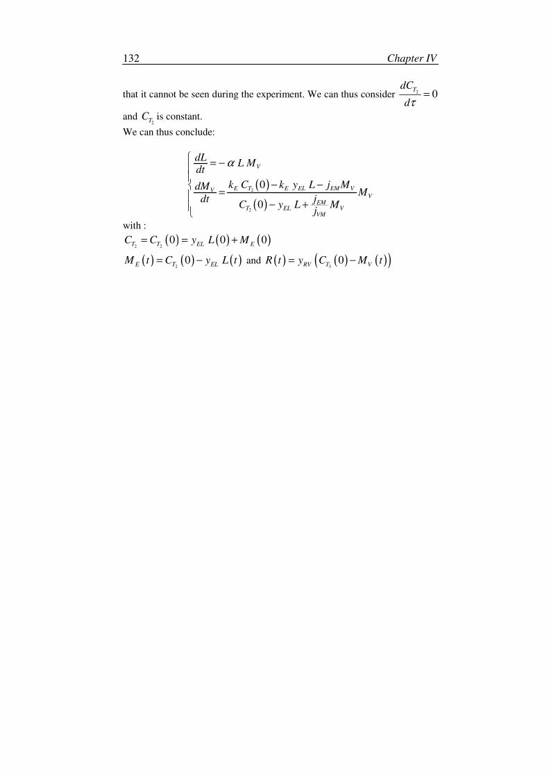
Chapter IV 132
that it cannot be seen during the experiment. We can thus consider 2 0TdC
dτ
=
and 2T
C is constant.
We can thus conclude:
( )
( )
2
2
0
0
V
E T E EL EM VVV
EMT EL V
VM
dLL M
dt
k C k y L j MdMM
dt jC y L M
j
α
= −
− −=
− +
with :
( ) ( ) ( )2 2
0 0 0T T EL EC C y L M= = +
( ) ( ) ( )2
0E T ELM t C y L t= − and ( ) ( ) ( )( )3
0RV T V
R t y C M t= −
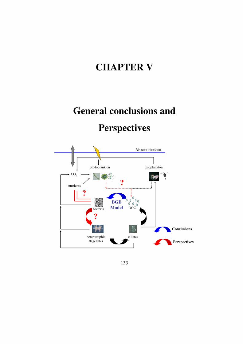
133
CHAPTER V
General conclusions and
Perspectives
phytoplankton zooplankton
bacteria
heterotrophic
flagellates
ciliates
DOC
CO2
nutrients
Air-sea interface
BGE
Model
?
?
?
Conclusions
Perspectives
Chapter V 134
I. Bacterial growth efficiency
This thesis highlighted several patterns in the dynamics of BGE.
Utilisation of the Monod model on in situ data has demonstrated that the
BGE varies according to depth and season, with higher values in surface
layer and during warm seasons (Eichinger et al., 2006 – chapter II). To our
knowledge, BGE variation with depth was never shown previously. The fact
that the BGE dynamic depends on the season, or on the temperatures, was
already demonstrated, but not by using a modelling approach.
The third chapter also deals with the BGE variability, but in artificial
culture conditions. The experiments were here carried out to determine the
influence of the input regime on bacterial and BGE dynamics. We have
demonstrated that the way of introducing the substrate in the batch has a
profound impact on the BGE value. The substrate quantity and quality were
the same in both experiments, they thus may not have an impact in this case.
The pulse experiment simulated a transient environment in terms of DOC
availability. We have shown that this kind of environment, closer to natural
environment from a qualitative point of view, is more efficient for bacterial
degradation than a constant environment, generally investigated to estimate
BGE. Consequently, the method of BGE estimation should be reviewed by
trying to incorporate more realistic substrate dynamics. However, our
experimental design is still far from natural conditions in terms of the amount
of substrate, and experimental efforts should be done to be closer to natural
DOC and bacterial concentrations.
Chapters II and III both used models to estimate the BGE. This method
seems suitable as we have proven in chapter II that BGE estimated from the
Monod model and from experimental data are qualitatively and quantitatively
equivalent. However, the BGE value estimated from models will of course
depend on the model used. The Monod model does not incorporate
maintenance process, and thus exhibits higher BGE values than models
which do. BGE estimation from Monod model seems to be closer to the
experimental estimation for both studies investigated in this thesis (chapters
II and III). As the Marr-Pirt and DEB models include maintenance, they
exhibit smaller BGE values than the Monod estimation. The BGE estimated
from the Marr-Pirt and the DEB models are very similar and considered as
equivalent. However, it is difficult from these results to determine which of
these estimations matches better with the “true” or “natural” BGE. The
diversity of methods used in BGE investigation makes BGE dynamics
difficult to study. This variability can only be demonstrated when BGE are
Conclusions and Perspectives 135
estimated with the same method in the same study. We may talk about an
“absolute” BGE. Indeed, even if BGE values are not identical with the
different methods, they always show the same pattern: smaller in deep waters
and during cold seasons, and smaller in a constant than in a transient
environment.
Nevertheless, a dynamic BGE could be investigated. Indeed, models
provide tools to represent experimental dynamics by implementing the
required processes. This tool could allow the representation of the BGE
dynamics during an experiment and thus highlighting events or processes
responsible for BGE changes. However, in this case the comparison between
several estimations is difficult as we should compare dynamics and not
individual BGE values. Nevertheless, this method should be considered.
II. Bacterial growth models
In this thesis, several bacterial growth models have been used and for
different purposes. The Monod model was used to describe bacterial growth
(1) from in situ data, as the data did not allowed the application of more
complex models, and also (2) from artificial culture data to test its pertinence
in transient conditions. The model matched the data well in the first case but
not in the second case, as experiments realised in artificial conditions were
carried out for a sufficient long time to exhibit biomass decrease which could
not be simulated by the Monod model due to the absence of maintenance.
Consequently, the adequacy of a model to describe data is primarily
determined by the type of data, and simple models can often be sufficient to
represent some dynamics.
The Marr-Pirt and DEB models were utilised in chapter III for
representing bacterial culture dynamics. The application of these models was
required as experimental data showed the presence of maintenance. Both
models equally fitted data, but we have also shown that the Marr-Pirt model
could be less efficient if the pulse experiment was realised in the conditions
of the batch experiment. This showed that the fit success may be determined
by the data set, and that only small variations in the experimental setup could
change the type of model that should be used. The advantage of the DEB
formulation is that it is more flexible and thus suitable in all cases, as it can
be reduced to Monod or Marr-Pirt models.
Chapter V 136
We also have demonstrated that the growth part of the Monod (chapter
II) and DEB (chapter IV) models may be simplified in a logistic equation,
with a constant and a variable carrying capacity, respectively. The utilisation
of this logistic equation reduces the model complexity in terms of calibration
and simulation costs, without affecting model performance. This
simplification step is required if we use these models in a biogeochemical
context. The key role of bacteria in the oceanic ecosystems has still been
proven and we have demonstrated in this study that they need to be modelled
accurately at the global level to obtain a good representation of the aquatic
carbon cycle. Once a suitable formulation has been found, it should be
simplified if this latter is complex in terms of number of parameters or state
variables with respect to the number of organisms or elements. Model
reduction facilitates calibration, simulation and understanding of the
underlying processes. However, model reduction should only be envisaged
when the complete model is constructed from experimental data, thus when
the complete model might provide realistic representation of experimental or
environmental dynamics.
III. Experimentation – modelling coupling
The conclusions of this thesis were possible because we coupled
experimentation and modelling. This coupling is essential to obtain realism.
For example, measurements made in chapter II (bacterial production and
respiration) did not demonstrate the maintenance that occurred in these
natural bacteria assemblages. Consequently, a model including maintenance
was not required. On the contrary, experiments carried out in artificial
conditions were specifically designed to place bacteria in starvation
conditions and highlight the necessity of the maintenance process in bacterial
modelling. Consequently, experiments should be planned in a modelling
framework. We won’t find an appropriate formulation for bacterial growth
without thinking before about which kind of processes they could implement.
Then, the experimental design can be prepared by planning which kind of
experiments and measurements should be used to quantify the various
processes. The utilisation of models also requires numerous data for the
calibration and validation, especially when dealing with transient
environments, as the pulse experiment of chapter III. Of course, this requires
a profound investment in terms of effort and finances. Then, model outputs
could serve to improve the sampling strategy, the type of measurements to be
made, the design of the future experiments. Chapter III discussed what
experiments could discriminate between the DEB and the Marr-Pirt models.
Conclusions and Perspectives 137
Consequently, the best strategy alternates repeatedly between experiment and
modelling.
Another important fact highlighted in this thesis is the necessity to use
artificial conditions to reveal key processes (chapter III). Indeed, the diversity
of uncertainties, when dealing with natural samples (chapter II), complicates
the analysis of results and makes the utilisation of complex model
inappropriate as processes are difficult to isolate from uncertainties. The
utilisation of artificial seawater and monospecific bacteria is of course far
from in situ conditions, but we first need a better understanding of the key
processes. Moreover, we can easily control external conditions and thus add
several limitations or introducing other organisms as we go along.
IV. Perspectives
My conclusions lead me to think that hypotheses asserted in this thesis
should be check experimentally. We have assumed that DOC accumulation
in batches (chapters III and IV) is due to its refractory nature. This
assumption could be check by measuring substrate (pyruvate) concentration
as well as DOC concentration in the cultures. However, we should first
improve our protocol of pyruvate detection. This kind of analysis is delicate
and not much used currently. Nevertheless, it will be probably feasible soon
with the method perfected by Tedetti et al. (2006) at LMGEM. We should
also measure N and P concentrations (or NH4+ and PO4
3- concentrations) to
be sure that the systems were not limited by inorganic nutrients. The
measurements of N and P, in the culture medium as well as in the bacterial
biomass, could also be useful for improving the DEB model. As done by
Martinussen and Thingstad (1987), we could so take into account three
reserves and have a more accurate idea on bacterial dynamics. Then, we
could test several limitations, for example by pulsing periodically two
nutrients (C and N or C and P), and then by pulsing the three of them (C, N
and P). We could so have more insights about bacterial physiology, for
example on the regulation of bacterial C:N and C:P ratios in transient
environments. The investigation of Thingstad (1987) showed that a Monod-
type model may effectively be sufficient in many purposes, but that a model
with a reserve for each kind of compound allows an easier incorporation of
biologically plausible concepts. In addition, the depletion areas, in function
of C:P and C:N ratios, of batch and chemostat cultures are accurately
represented by this model with three reserves (Martinussen & Thingstad
1987). This kind of approach would also allow a better understanding about
Chapter V 138
the storage capacity, and test the prediction of DEB theory that nutrient
reserves accumulate under energy limitation. Nevertheless, the addition of all
of these measurements needs an improvement of the experimental protocol,
since the time required for doing all carbon measurements carried out in this
thesis was already substantial, and the addition of other measurements would
imply either a reduction of the number of data points between two pulses, or
another experimental design.
One of the solutions would be the utilisation of chemostats instead of
batch systems. The culture volume that is required to perform all
measurements is a point of concern. The sampling protocol could so be
automated. To mimic transient environments we should vary either the
dilution rate or the substrate concentration in the input.
The real complexity of the natural medium let me suggest that it is
necessary to test prey-predator interactions in the context of the DEB theory.
Kooi and Kooijman (1994) showed the necessity of adding a storage
compartment as well as the maintenance process to the Monod model for
representing data of a trophic chain implying one substrate, one bacterial
species and one predator. We could imagine the same kind of protocol by
pulsing the substrate. The model should include the DOC production by the
predator (grazer), and it would thus comprise two DOC sources (the input
substrate as well as DOC produced from grazing), with a differentiate
preference in the uptake. In the DEB context, the grazer would have two
nutritive sources: bacterial reserve and structure. In the same way, we could
test an interaction between a phytoplankton and bacterial species. Bratbak
and Thingstad (1985) tested this kind of interaction with chemostat
experiments, where the nutritive resource was phosphate, and showed that
bacterial density increased whereas phytoplankton density decreased at low
dilution rates. They have also constructed a model where both organisms are
in competition for the limiting resource but where the phytoplankton
produces organic carbon assimilated by bacteria. This approach could be
used by including more realist nutrient dynamics, as the pulse input of
substrate in this thesis. The model should thus include two DOC sources and
bacteria would compete for the inorganic nutrients with phytoplankton. Then,
we could test the effect of these processes in a biogeochemical model, after
having simplified their formulation.
To sum up, more coupling between experimental and modelling work
should be investigated. In the bacterial context, studies that deal with both
approaches at the same time are seldom. Some investigations succeed to
Conclusions and Perspectives 139
demonstrate experimentally some theoretical results obtained few decades
earlier. For example, the study of Becks et al. (2005) demonstrated the
existence of chaotic behaviour in a microbial food web with chemostat
experiments. The existence of chaos in simple ecological systems was
however demonstrated with models since a long time. In this thesis, model
comparison with experimental data (chapter III) showed that a complex
model is not currently necessary to represent bacterial dynamics in a pulse
DOC environment. Nevertheless, models provide tools to test assumptions
and/or the influence of the addition of processes in system dynamics. In this
context, the influence of the incorporation of physiological details in
ecosystem models on global dynamics could be tested. For example, we can
test the DEB formulations on the 1-D model of Anderson & Williams (1999),
which simulates the DOC distribution in the water column, by keeping the
same global model structure. Then, we can observe if these detailed
formulations imply dynamical differences and judge the necessity of using
mechanistic models at the global scale.

140
141
References
Amon RMW, Benner R (1996) Bacterial utilization of different size classes
of dissolved organic matter. Limnology and Oceanography 41:41-51
Anderson TR, Ducklow HW (2001) Microbial loop carbon cycling in ocean
environments studied using a simple steady-state model. Aquatic
Microbial Ecology 26:37-49
Anderson TR, Williams PJleB (1998) Modelling the seasonal cycle of
dissolved organic carbon at station E-1 in the English Channel.
Estuarine Coastal and Shelf Science 46:93-109
Anderson TR, Williams PJleB (1999) A one-dimensional model of dissolved
organic carbon cycling in the water column incorporating combined
biological-photochemical decomposition. Global Biogeochemical
Cycles 13:337-349
Arhonditsis GB, Brett MT (2004) Evaluation of the current state of
mechanistic aquatic biogeochemical modeling. Marine Ecology-
Progress Series 271:13-26
Azam F, Fenchel T, Field JG, Gray JS, Meyer-Reil LA, Thingstad TF
(1983) The ecological role of water-column microbes in the
sea. Marine Ecology-Progress Series 10:257-263
Baird ME, Walker SJ, Wallace BB, Webster IT, Parslow JS (2003) The use
of mechanistic descriptions of algal growth and zooplankton grazing
in an estuarine eutrophication model. Estuarine Coastal and Shelf
Science 56:685-695
Baklouti M, Diaz F, Pinazo C, Faure V, Queguiner B (2006a) Investigation
of mechanistic formulations depicting phytoplankton dynamics for
models of marine pelagic ecosystems and description of a new
model. Progress in Oceanography 71:1-33
Baklouti M, Faure V, Pawlowski L, Sciandra A (2006b) Investigation and
sensitivity analysis of a mechanistic phytoplankton model
implemented in a new modular numerical tool (Eco3M) dedicated to
biogeochemical modelling. Progress in Oceanography 71:34-58
References 142
Baretta-Bekker JG, Baretta JW, Hansen AS, Riemann B (1998) An improved
model of carbon and nutrient dynamics in the microbial food web in
marine enclosures. Aquatic Microbial Ecology 14:91-108
Baretta-Bekker JG, Baretta JW, Rasmussen EK (1995) The microbial food
web in the European Regional Seas Ecosystem Model. Netherland
Journal of Sea Research 33:363-379
Baretta-Bekker JG, Riemann B, Baretta JW, Koch Rasmussen E (1994)
Testing the microbial loop concept by comparing mesocosm data
with results from a dynamical simulation model Marine Ecology-
Progress Series 106:187-198
Bauer JE, Williams PM, Druffel ERM (1992) C-14 Activity of Dissolved
Organic-Carbon Fractions in the North-Central Pacific and Sargasso
Sea. Nature 357:667-670
Baxter M, Sieburth JMN (1984) Metabolic and ultrastructural response to
glucose of two eurytrophic bacteria isolated from seawater at
different enriching concentrations. Applied and Environmental
Microbiology 47:31-38
Becks L, Hilker FM, Malchow H, Jürgens K, Arndt H (2005) Experimental
demonstration of chaos in microbial foo web. Nature 435:1226-1229
Bendtsen J, Lundsgaard C, Middelboe M, Archer D (2002) Influence of
bacterial uptake on deep-ocean dissolved organic carbon. Global
Biogeochemical Cycles 16:Art. No. 1127
Billen G, Becquevort S (1991) Phytoplankton Bacteria Relationship in the
Antarctic Marine Ecosystem. Polar Research 10:245-253
Bissett WP, Walsh JJ, Dieterle DA, Carder KL (1999) Carbon cycling in the
upper waters of the Sargasso Sea: I. Numerical simulation of
differential carbon and nitrogen fluxes. Deep-Sea Research Part I -
oceanographic research papers 46:205-269
Blackburn N, Zweifel UL, Hagstrom A (1996) Cycling of marine dissolved
organic matter .II. A model analysis. Aquatic Microbial Ecology
11:79-90
Brandt BW, Kelpin FDL, van Leeuwen IMM, Kooijman SALM (2004)
Modelling microbial adaptation to changing availability of substrates.
Water Research 38:1003-1013
Brandt BW, van Leeuwen IMM, Kooijman SALM (2003) A general model
for multiple substrate biodegradation. Application to co-metabolism
References 143
of structurally non-analogous compounds. Water Research 37:4843-
4854
Briand E, Pringault O, Jacquet S, Torréton P (2004) The use of oxygen
microprobes to measure bacterial respiration for determining
bacterioplankton growth efficiency. Limnology and Oceanography:
Methods 2:406-416
Cajal-Medrano R, Maske H (1999) Growth efficiency, growth rate and the
remineralization of organic substrate by bacterioplankton - revisiting
the Pirt model. Aquatic Microbial Ecology 19:119-128
Cajal-Medrano R, Maske H (2005) Growth efficiency and respiration at
different growth rates in glucose-limited chemostats with natural
marine bacteria populations. Aquatic Microbial Ecology 38:125-133
Carlson CA (2002) Production and removal processes. In: Hansell DA,
Carlson CA (eds) Biogeogemistry of marine dissolved organic
matter. Academic Press, San Diego, p 91-151
Carlson CA, Bates NR, Ducklow HW, Hansell DA (1999) Estimation of
bacterial respiration and growth efficiency in the Ross Sea,
Antarctica. Aquatic Microbial Ecology 19:229-244
Carlson CA, Ducklow HW (1995) Dissolved organic carbonin the upper
ocean of the central equatorial Pacific Ocean, 1992: Daily and
finescale vertical variations. Deep-Sea Research Part II-Topical
Studies in Oceanography 42:639-656
Carlson CA, Ducklow HW (1996) Growth of bacterioplankton and
consumption of dissolved organic carbon in the Sargasso Sea.
Aquatic Microbial Ecology 10:69-85
Carlson CA, Ducklow HW, Hansell DA, Smith WO Jr (1998) Organic
carbon partitioning during spring phytoplancton blooms in the Ross
Sea polynya and the Sargasso Sea. Limnology and Oceanography
43:375-386
Carlson CA, Giovannoni SJ, Hansell DA, Goldberg SJ, Parsons R, Otero MP,
Vergin K, Wheeler BR (2002) Effect of nutrient amendments on
bacterioplankton production, community structure, and DOC
utilization in the northwestern Sargasso Sea. Aquatic Microbial
Ecology 30:19-36
Carlson CA, Giovannoni SJ, Hansell DA, Goldberg SJ, Parsons R, Vergin K
(2004) Interactions among dissolved organic carbon, microbial
processes, and community structure in the mesopelagic zone of the
References 144
northwestern Sargasso Sea. Limnology and Oceanography 49:1073-
1083
Cherrier J, Bauer JE (2004) Bacterial utilization of transient plankton-derived
dissolved organic carbon and nitrogen inputs in surface ocean waters.
Aquatic Microbial Ecology 35:229-241
Cherrier J, Bauer JE, Druffel ERM (1996) Utilization and turnover of labile
dissolved organic matter by bacterial heterotrophs in eastern north
Pacific surface waters. Marine Ecology-Progress Series 139:267-279
Christian JR, Anderson TR (2002) Modeling DOM biogeochemistry. In:
Hansell DA, Carlson CA (eds) Biogeochemistry of marine dissolved
organic matter. Academic Press, London, p 774
Coffin RB, Connolly JP, Harris PS (1993) Availability of dissolved organic
carbon to bacterioplankton examined by oxygen utilization. Marine
Ecology-Progress Series 101:9-22
Connolly JP, Coffin RB (1995) Model of Carbon Cycling in Planktonic Food
Webs. Journal of Environmental Engineering-Asce 121:682-690
Copinmontegut G, Avril B (1993) Vertical-Distribution and Temporal
Variation of Dissolved Organic-Carbon in the North-Western
Mediterranean-Sea. Deep-Sea Research Part I-Oceanographic
Research Papers 40:1963-1972
Dafner E, Gonzalez-Davila M, Santana-Casiano JM, Sempéré R (2001) Total
organic and inorganic carbon exchange through the Strait of
Gibraltar in September 1997. Deep-Sea Research Part I-
Oceanographic Research Papers 48:1217-1235
Davidson K (1996) Modelling microbial food webs. Marine Ecology-
Progress Series 145:279-296
Dearman JR, Taylor AH, Davidson K (2003) Influence of autotroph model
complexity on simulations of microbial communities in marine
mesocosms. Marine Ecology-Progress Series 250:13-28
del Giorgio PA, Cole JJ (1998) Bacterial growth efficiency in natural aquatic
systems. Annual Review of Ecology and Systematics 29:503-541
del Giorgio PA, Duarte CM (2002) Respiration in the open ocean. Nature
420:379-384
Droop MR (1968) Vitamin B12 and marine ecology. IV. The kinetics of
uptake, growth and inhibition in Monochrysis lutheri. Journal of the
Marine Biological Association of the United Kingdom 48:689-733
References 145
Druffel ERM, Williams PM, Bauer JE, Ertel JR (1992) Cycling of Dissolved
and Particulate Organic-Matter in the Open Ocean. Journal of
Geophysical Research-Oceans 97:15639-15659
Ducklow H, Carlson C, Smith W (1999) Bacterial growth in experimental
plankton assemblages and seawater cultures from the Phaeocystis
antarctica bloom in the Ross Sea, Antarctica. Aquatic Microbial
Ecology 19:215-227
Ducklow HW, Carlson CA (1992) Oceanic Bacterial Production. Advances
in Microbial Ecology 12:113-181
Eichinger M, Kooijman SALM, Sempéré R, Poggiale JC (submitted)
Mechanistic model simplification for implementation in
biogeochemical models: case of bacterial DOC degradation in a
perturbed system. Ecological Modelling
Eichinger M, Poggiale JC, Van Wambeke F, Lefèvre D, Sempéré R (2006)
Modelling DOC assimilation and bacterial growth efficiency in
biodegradation experiments: a case study in the Northeast Atlantic
Ocean. Aquatic Microbial Ecology 43:139-151
Fagerbakke KJ, Heldal M, Norland S (1996) Content of carbon, nitrogen,
oxygen, sulfur and phosphorus in native aquatic and cultured
bacteria. Aquatic Microbial Ecology 10:15-27
Farjalla VF, Azevedo DA, Esteves FA, Bozelli RL, Roland F, Enrich-Prast A
(2006) Influence of hydrological pulse on bacterial growth and DOC
uptake in a clear-water Amazonian lake. Microbial Ecology 52:334-
344
Farrington J (1992) Overview and key recommendations. Marine organic
geochemistry workshop, January 1990. Marine Chemistry 39:5-9
Flynn KJ (2005) Castles built on sand: dysfunctionality in plankton models
and the inadequacy of dialogue between biologists and modellers.
Journal of Plankton Research 27:1205-1210
Fujii M, Murashige S, Ohnishi Y, Yuzawa A, Miyasaka H, Suzuki Y,
Komiyama H (2002) Decomposition of phytoplankton in seawater.
Part 1: Kinetic analysis of the effect of organic matter concentration.
Journal of Oceanography 58:433-438
Fulton EA, Parslow JS, Smith ADM, Johnson CR (2004) Biogeochemical
marine ecosystem models II: the effect of physiological detail on
model performance. Ecological Modelling 173:371-406
References 146
Goldman JC, Caron DA, Dennett MR (1987) Regulation of gross growth
efficiency and ammonium regeneration in bacteria by susbtrate C:N
ratio. Limnology and Oceanography 32:1239-1252
González N, Anadón R, Marañón E (2002) Large-scale variability of
planktonic net community metabolism in the Atlantic Ocean:
importance of temporal changes in oligotrophic subtropical waters.
Marine Ecology-Progress Series 233
Grossart HP, Simon M (2007) Interactions of planktonic algae and bacteria:
effects on algal growth and organic matter dynamics. Aquatic
Microbial Ecology 47:163-176
Grover JP (1991) Resource Competition in a Variable Environment -
Phytoplankton Growing According to the Variable-Internal-Stores
Model. American Naturalist 138:811-835
Guidi L, Stemman L, Legendre L, Picheral M, Prieur L, Gorsky G (2007)
Vertical distribution of aggregates (> 110 µm) and mesoscale activity
in the northeastern Atlantic: Effects on the deep vertical export of
surface carbon. Limnology and Oceanography 52:7-18
Guven B, Howard A (2007) Identifying the critical parameters of a
cyanobacterial growth and movement model by using generalised
sensitivity analysis. Ecological Modelling 207:11-21
Hanegraaf PPF (1997) Mass and energy fluxes in microorganisms according
to the Dynamic Energy udget theory for filaments. Vrije Universiteit,
Amsterdam
Hanegraaf PPF, Kooi BW (2002) The dynamics of a tri-trophic food chain
with two-component populations from a biochemical perspective.
Ecological Modelling 152:47-64
Hanegraaf PPF, Muller EB (2001) The dynamics of the macromolecular
composition of biomass. Journal of theoretical biology 212:237-251
Hansell DA (2002) DOC in the global ocean carbon cycle. In: Hansell DA,
Carlson CA (eds) Biogeochemistry of marine dissolved organic
matter. Academic Press, London, p 774
Hansell DA, Bates NR, Gundersen K (1995) Mineralization of dissolved
organic carbon in the Sargasso Sea. Marine Chemistry 51:201-212
Hansell DA, Carlson CA (1998a) Deep-ocean gradients in the concentration
of dissolved organic carbon. Nature 395:263-266
References 147
Hansell DA, Peltzer ET (1998) Spatial and temporal variations of total
organic carbon in the Arabian Sea. Deep-Sea Research Part Ii-
Topical Studies in Oceanography 45:2171-2193
Harvey HR, Tuttle JH, Bell JT (1995) Kinetics of Phytoplankton Decay
during Simulated Sedimentation - Changes in Biochemical-
Composition and Microbial Activity under Oxic and Anoxic
Conditions. Geochimica Et Cosmochimica Acta 59:3367-3377
Hedges JI (1992) Global biogeochemical cycles: Progress and problems.
Marine Chemistry 39:67-93
Heldal M, Norland S, Fagerbakke KJ, Thingstad TF, Bratbak G (1996) The
elemental composition of bacteria: a signature of growth conditions?
Marine Pollution Bulletin 33:3-9
Herbert D (1958) Some principles of continuous culture. In: Tunevall
G (ed) Recent progress in microbiology, Vol 7. Almquist and
Wiksell, Stockholm, p 381–396
Iwasa Y, Levin SA, Andreasen V (1989) Aggregation in Model-Ecosystems
.2. Approximate Aggregation. Ima Journal of Mathematics Applied
in Medicine and Biology 6:1-23
Jahnke RA, Craven DB (1995) Quantifying the Role of Heterotrophic
Bacteria in the Carbon-Cycle - a Need for Respiration Rate
Measurements. Limnology and Oceanography 40:436-441
Jorgensen NOG, Kroer N, Coffin RB, Hoch MP (1999) Relations between
bacterial nitrogen metabolism and growth efficiency in an estuarine
and an open-water ecosystem. Aquatic Microbial Ecology 18:247-
261
Karayanni H, Christaki U, Van Wambeke F, Denis M, Moutin T (2005)
Influence of ciliated protozoa and heterotrophic nanoflagellates on
the fate of primary production in the northeast Atlantic Ocean.
Journal of Geophysical Research-Oceans 110: Art. No. C07S15
Kirchman DL (1993) Leucine incorporation as a measure of biomass
production by heterotrophic bacteria. In: Kemp PF, Cole JJ, Sherr
BF, Sherr EB (eds) Handbook of Methods in Aquatic Microbial
Ecology. Lewis Press, New York, p 509-512
Konopka A (1999) Theoretical analysis of the starvation response under
substrate pulses. Microbial Ecology 38:321-329
References 148
Kooi BW, Kooijman SALM (1994) The Transient-Behavior of Food-Chains
in Chemostats. Journal of Theoretical Biology 170:87-94
Kooijman SALM (2000) Dynamic Energy and Mass Budgets in Biological
Systems, Vol. Cambridge University Press, Cambridge
Kooijman SALM, Kooi BW, Hallam TG (1999) The application of mass and
energy conservation laws in physiologically structured population
models of heterotrophic organisms. Journal of Theoretical Biology
197:371-392
Kooijman SALM, Muller EB, Stouthamer AH (1991) Microbial growth
dynamics on the basis of individual budgets. Antonie Van
Leeuwenhoek 60:159-174
Kooijman SALM, Troost TA (2007) Quantitative steps in the
evolution of metabolic organisation as specified by the
dynamic energy budget theory. Biological Reviews 82:1-30
La Ferla R, Azzaro F, Azzaro M, Caruso G, Decembrini F, Leonardi M,
Maimone G, Monticelli LS, Raffa F, Santinelli C, Zaccone R, Ribera
d’Alcalá M (2005) Microbial contribution to carbon biogeochemistry
in the Central Mediterranean Sea: Variability of activities and
biomass. Journal of Marine Systems 57:146-166
Lagaria JC, Reeds JA, Wright MH, Wright PE (1998) Convergence
properties of the Nelder-Mead simplex method in low dimensions.
SIAM journal of optimization 9:112-147
Lancelot C, Staneva J, Van Eeckhout D, Beckers JM, Stanev E (2002)
Modelling the Danube-influenced north-western continental shelf of
the Black Sea. II: Ecosystem response to changes in nutrient delivery
by the Danube River after its damming in 1972. Estuarine Coastal
and Shelf Science 54:473-499
Lawrie J, Hearne J (2007) Reducing model complexity via output sensitivity.
Ecological Modelling 207:137-144
Lee S, Fuhrman JA (1987) Relationships between Biovolume and Biomass of
Naturally Derived Marine Bacterioplankton. Applied and
Environmental Microbiology 53:1298-1303
Legendre L, Rassoulzadegan F (1995) Plankton and nutrient dynamics in
marine waters. Ophelia 41:153-172
Lyman J., Fleming R. (1940) Composition of sea water. Journal of Marine
Research 3:134-146
References 149
Maixandeau A, Lefèvre D, Fernandez IC, Sempéré R, Sohrin R, Ras J, Van
Wambeke F, Caniaux G, Quéguiner B (2005) Mesoscale and
seasonal variability of community production and respiration in the
surface waters of the NE Atlantic Ocean. Deep-Sea Research Part I-
Oceanographic Research Papers 52:1663-1676
Marr AG, Nilson EH, Clark DJ (1963) The maintenance requirement of
Escherishia coli. Annals of the New York Academy of Sciences
102:536-548
Martinussen I, Thingstad TF (1987) Utilization of Organic-N, Organic-P and
Organic-C by Heterotrophic Bacteria .II. Comparison of Experiments
and a Mathematical-Model. Marine Ecology-Progress Series 37:285-
293
Mcmanus GB, Peterson WT (1988) Bacterioplankton Production in the
Nearshore Zone during Upwelling Off Central Chile. Marine
Ecology-Progress Series 43:11-17
Memery L, Reverdin G, Paillet J, Oschlies A (2005) Introduction to the
POMME special section: Thermocline ventilation and
biogeochemical tracer distribution in the northeast Atlantic Ocean
and impact of mesoscale dynamics. Journal of Geophysical
Research-Oceans 110: Art. No. C07S01
Merien D (2003) Variabilité biooptique à différentes échelles spatiales et
temporelles dans l'Atlantique nord-est: interprétations
biogéochimiques. University of Pierre and Marie Curie (Paris VI)
Michaelis L, Menten ML (1913) Die Kinetik der Invertinwirkung. Biochem.
Z. 49:333-369
Middelboe M, Jorgensen NOG, Kroer N (1996) Effects of viruses on nutrient
turnover and growth efficiency of noninfected marine
bacterioplankton. Applied and Environmental Microbiology
62:1991-1997
Miki T, Yamamura N (2005a) Effects of asynchronous fluctuations in DOC
supply and bacterial growth on biodegradation efficiency. Ecological
Modelling 183:281-299
Miki T, Yamamura N (2005b) Theoretical model of interactions between
particle-associated and free-living bacteria to predict functional
composition and succession in bacterial communities. Aquatic
Microbial Ecology 39:35-46
References 150
Mladenov N, McKnight DM, Wolski P, Murray-Hudson M (2007)
Simulation of DOM fluxes in a seasonal floodplain of the Okavango
Delta, Botswana. Ecological Modelling 205:181-195
Mladenov N, McKnight DM, Wolski P, Ramberg L (2005) Effects of annual
flooding on dissolved organic carbon dynamics within a pristine
wetland, the Okavango Delta, Botswana. Wetlands 25:622-638
Monfort P, Baleux B (1992) Comparison of flow cytometry and
epifluorescence microscopy for counting bacteria in aquatic ecosys
terns. Cytometry 13:188-192
Monod J (1942) Recherches sur la croissance des cultures bactériennes.
University of Paris
Murray AG, Parslow JS (1999) The analysis of alternative formulations in a
simple model of a coastal ecosystem. Ecological Modelling 119:149-
166
Nagata T (2000) Production mechanisms of dissolved organic matter. In:
Kirchman DL (ed) Microbial ecology of the oceans. Wiley-Liss, p
121-152
Nagata T, Kirchman DL (1999) Bacterial mortality: A pathway for the
formation of refractory DOM? In: Brylinsky M, Bell C, Johnson-
Grenn P (eds) New frontiers in Microbial Ecology: Proceedings of
the Eighth International Symposium on Microbial Ecology. Atlantic
Canda Society for Microbial Ecology, Halifax
Nisbet RM, Muller EB, Lika K, Kooijman SALM (2000) From molecules to
ecosystems through dynamic energy budget models. Journal of
Animal Ecology 69:913-926
Pahlow M, Vézina AF (2003) Adaptative model of DOM dynamics in the
surface ocean. Journal of Marine Research 61:127-146
Panagiotopoulos C, Sempéré R, Obernosterer I, Striby L, Goutx M, Van
Wambeke F, Gautier S, Lafont R (2002) Bacterial degradation of
large particles in the southern Indian Ocean using in vitro incubation
experiments. Organic Geochemistry 33:985-1000
Pirt SJ (1965) The maintenance energy of bacteria in growing cultures.
Proceedings of the Royal Society of London. Series B: Biological
Sciences 163:224-231
Poggiale JC, Auger P, Nerini D, Mante C, Gilbert F (2005) Global
production increased by spatial heterogeneity in a population
dynamics model. Acta Biotheoretica 53:359-370
References 151
Pomeroy LR (1974) The ocean's food web, a changing paradigm. Bioscience
24:499-504
Pomeroy LR, Sheldon JE, Sheldon WM, Peters F (1995) Limits to Growth
and Respiration of Bacterioplankton in the Gulf-of-Mexico. Marine
Ecology-Progress Series 117:259-268
Raguénès GHC, Peres A, Ruimy R, Pignet P, Christen R, Loaec M,
Rougeaux H, Barbier G, Guezennec JG (1997) Alteromonas infernus
sp. nov., a new polysaccharide-producing bacterium isolated from a
deep-sea hydrothermal vent. Journal of Applied Microbiology
82:422-430
Raick C, Delhez EJM, Soetaert K, Gregoire M (2005) Study of the seasonal
cycle of the biogeochemical processes in the Ligurian Sea using a 1D
interdisciplinary model. Journal of Marine Systems 55:177-203
Raick C, Soetaert K, Gregoire M (2006) Model complexity and performance:
How far can we simplify? Progress in Oceanography 70:27-57
Reinthaler T, Herndl GJ (2005) Seasonal dynamics of bacterial growth
efficiencies in relation to phytoplankton in the southern North Sea.
Aquatic Microbial Ecology 39:7-16
Rivkin RB, Legendre L (2001) Biogenic carbon cycling in the upper ocean:
Effects of microbial respiration. Science 291:2398-2400
Saunders G (1976) Decomposition in fresh water. In: Anderson J, Macfadyen
A (eds) The role of terrestrial and aquatic organisms in
decomposition processes. Blackwell, p 341-374
Sempéré R, Dafner E, Van Wambeke F, Lefèvre D, Magen C, Allegre S,
Bruyant F, Bianchi M, Prieur L (2003) Distribution and cycling of
total organic carbon across the Almeria-Oran Front in the
Mediterranean Sea: Implications for carbon cycling in the western
basin. Journal of Geophysical Research-Oceans 108:Art. No. 3361
Sempéré R, Van Wambeke F, Azourmanian H, Chambaut AL, Ferrière L,
Bianchi M (1998) On the use of batch systems to determine DOC
bacterial lability and bacterial growth efficiency in seawater samples.
In: Bayens J, Dehairs F, Goyens, L (eds) Inetgrated marine system
analysis. European Network for integrated Marine System Analysis,
p 233-238
Sempéré R, Yoro SC, Van Wambeke F, Charrière B (2000) Microbial
decomposition of large organic particles in the northwestern
References 152
Mediterranean Sea: an experimental approach. Marine Ecology-
Progress Series 198:61-72
Sherr EB, Sherr BF (1996) Temporal offset in oceanic production and
respiration processes implied by seasonal changes in atmospheric
oxygen: The role of heterotrophic microbes. Aquatic Microbial
Ecology 11:91-100
Siegenthaler U, Sarmiento JL (1993) Atmospheric Carbon-Dioxide and the
Ocean. Nature 365:119-125
Sohrin R, Sempéré R (2005) Seasonal variation in total organic carbon in the
northeast Atlantic in 2000-2001. Journal of Geophysical Research-
Oceans 110:-
Spitz YH, Moisan JR, Abbott MR (2001) Configuring an ecosystem model
using data from the Bermuda Atlantic Time Series (BATS). Deep-
Sea Research Part II-Topical Studies in Oceanography 48:1733-1768
Talin F, Tolla C, Rabouille C, Poggiale JC (2003) Relations between
bacterial biomass and carbon cycle in marine sediments: An early
diagenetic model. Acta Biotheoretica 51:295-315
Taylor AH, Joint I (1990) A Steady-State Analysis of the Microbial Loop in
Stratified Systems. Marine Ecology-Progress Series 59:1-17
Tedetti M, Kawamura K, Charrière B, Chevalier N, Sempéré R (2006)
Determination of low molecular weight dicarboxylic and
ketocarboxylic acids in seawater samples. Analytical Chemistry
78:6012-6018
Tedetti M, Kawamura K, Narukawa M, Joux F, Charrière B, Sempéré R
(2007) Hydroxyl radical-induced photochemical formation of
dicarboxylic acids from unsaturated fatty acid (oleic acid) in aqueous
solution. Journal of Photochemistry and Photobiology a-Chemistry
188:135-139
Thingstad TF (1987) Utilization of N, P, and Organic C by Heterotrophic
Bacteria .I. Outline of a Chemostat Theory with a Consistent Concept
of Maintenance Metabolism. Marine Ecology-Progress Series 35:99-
109
Thingstad TF, Pengerud B (1985) Fate and Effect of Allochthonous Organic
Material in Aquatic Microbial Ecosystems - an Analysis Based on
Chemostat Theory. Marine Ecology-Progress Series 21:47-62
Tian RC, Vézina AF, Legendre L, Ingram RG, Klein B, Packard T, Roy S,
Savenkoff C, Silverberg N, Therriault J-C, Tremblay J-E (2000)
References 153
Effects of pelagic food-web interactions and nutrient
remineralization on the biogeochemical cycling of carbon: a
modelling approach. Deep-Sea Research Part II-Topical Studies in
Oceanography 47:637-662
Tolla C, Kooijman SALM, Poggiale JC (2007) A kinetic inhibition
mechanism for maintenance. Journal of Theoretical Biology
244:576-587
Touratier F, Legendre L, Vezina A (1999) Model of bacterial growth
influenced by substrate C:N ratio and concentration. Aquatic
Microbial Ecology 19:105-118
Vallino JJ (2000) Improving marine ecosystem models: Use of data
assimilation and mesocosm experiments. Journal of Marine Research
58:117-164
Vallino JJ, Hopkinson CS, Hobbie JE (1996) Modeling bacterial utilization
of dissolved organic matter: optimization replaces Monod growth
kinetics. Limnology and Oceanography 41:1591-1609
Verdugo P, Alldredge AL, Azam F, Kirchman DL, Passow U, Santschi PH
(2004) The oceanic gel phase: a bridge in the DOM–POM
continuum. Marine Chemistry 92:67-85
Vichi M, Oddo P, Zavatarelli M, Coluccelli A, Coppini G, Celio M, Umani
SF, Pinardi N (2003) Calibration and validation of a one-dimensional
complex marine biogeochemical flux model in different areas of the
northern Adriatic shelf. Annales Geophysicae 21:413-436
Vrede K, Heldal M, Norland S, Bratbak G (2002) Elemental composition (C,
N, P) and cell volume of exponentially growing and nutrient-limited
bacterioplankton. Applied and Environmental Microbiology
68:2965-2971
Wheeler PA, Gosselin M, Sherr E, Thibault D, Kirchman DL, Benner R,
Whitledge TE (1996) Active cycling of organic carbon in the central
Arctic Ocean. Nature 380:697-699
Wiebinga CJ, de Baar HJW (1998) Determination of the distribution of
dissolved organic carbon in the Indian sector of the Southern Ocean.
Marine Chemistry 61:185-201
Williams PJleB, Jenkinson NW (1982) A Transportable Microprocessor-
Controlled Precise Winkler Titration Suitable for Field Station and
Shipboard Use. Limnology and Oceanography 27:576-584

References 154
Williams PJleB (2000) Heterotrophic bacteria and the dynamics of dissolved
organic material. In: Kirchman DL (ed) Microbial ecology of the
oceans. Wiley-Liss, p 153-199
Williams PM, Druffel ERM (1987) Radiocarbon in Dissolved Organic-
Matter in the Central North Pacific-Ocean. Nature 330:246-248
Yoro SC, Panagiotopoulos C, Sempéré R (1999) Dissolved organic carbon
contamination induced by filters and storage bottles. Water Research
33:1956-1959
Zweifel UL, Norrman B, Hagstrom A (1993) Consumption of Dissolved
Organic-Carbon by Marine-Bacteria and Demand for Inorganic
Nutrients. Marine Ecology-Progress Series 101:23-32
155
Summary
Bacterial degradation of dissolved organic carbon in
the water column
An experimental and modelling approach
This thesis deals with the growth of heterotrophic pelagic bacteria which
use the dissolved organic carbon (DOC) as nutritive resource. It is widely
recognised that heterotrophic bacteria play a predominant role in the carbon
cycle. Indeed, they represent the most important living biomass in aquatic
ecosystems and constitute the major DOC consumers. DOC is the second
most important stock of bioreactive carbon in ocean and its dynamics are
important for understanding the global carbon cycle and changes of
atmospheric CO2. DOC may play an important role in the biogeochemistry of
the oceanic carbon cycle as it contributes to the biological pump by the
export of sinking biogenic particles. The carbon flow through the bacterial
compartment is investigated by the bacterial growth efficiency (BGE). BGE
provides an estimation of the DOC fraction that is used by bacteria for their
growth, the rest being remineralised. Numerous studies investigated the
influence of environmental factors on BGE values. These factors generally
comprise temperature, season, distance from the shore and substrate quality.
This thesis aims to investigate heterotrophic bacterial growth by using
both experimental and modelling approaches. The experimental work used
natural as well as artificial seawater. Various models for bacterial growth,
comprising different levels of complexity, were investigated to represent
mathematically the dynamics of the different experiments. Two main axes
merge in this work: (1) the study of growth models, constructed from
experimental results, with a view to implement them in ecosystem models,
and (2) the investigation of the environmental factors influencing the BGE
with these models. The main objective consists of the study of bacterial
growth in different environmental contexts and to deduce a suitable
mathematical formulation for describing the interaction between growth and
DOC to include this in a biogeochemical model later on.
Summary 156
We first studied bacterial and DOC dynamics from in situ samples.
Numerous biodegradation experiments, implying natural DOC and bacterial
assemblages, were realised in stable conditions in the Northeast Atlantic
Ocean according to several seasons and depths. We utilised the Monod model
for representing the data acquired during these experiments. This model is
empirical, constructed with Michaelis-Menten kinetics and is the most widely
used for describing bacterial growth in ecosystem models. BGE was
estimated experimentally, as generally done by most authors, and also by
using the model. We demonstrated that BGE varies according to season and
depth, the dynamics being the same with both methods of estimation. As
BGE is one parameter of the Monod model, this result proved that it is
inaccurate for representing the utilisation of DOC by bacteria in ecosystem
models.
We then decided to carry out experiments in artificial conditions, with a
monospecific bacterial strain and a single DOC substrate. This setup provides
data sets that are easier to analyse and allows the application of more
complex models. To test the performance of several models, comprising
several levels of complexity, including the Monod model, 2 kinds of
experiments were performed: 1 experiment was realised in constant
conditions with a single substrate load at the start of the experiment, as the
previous study, the other experiment was carried out by pulsing the substrate
supply periodically. The total amount of substrate was the same in both
experiments, the only difference consists of the input regime. The substrate
pulses mimic the spatial and temporal variability of DOC distribution. We
demonstrated that the Monod model is inaccurate to represent bacterial
dynamics when they are in starved conditions, which may often occur in
natural environments. We also utilised a model implementing the bacterial
maintenance, the Marr-Pirt model, and another model, constructed from the
dynamic energy budget (DEB) theory, including maintenance as well as a
reserve compartment. Both models match the data very well. However, the
DEB model, due to its mechanistic basis, is more flexible and is able to adapt
to more situations. BGE was estimated experimentally and with the 3 models
for both experiments. We demonstrated that BGE is higher in the pulse
experiment than in the experiment carried out in stable conditions with all
methods of BGE estimation. Consequently, the spatial and temporal
variability of DOC distribution has a profound impact on the estimation of
BGE value.
Data of the pulse experiment were also used to formulate a mechanistic
model, based on the DEB theory as stated previously. In a third section, we
investigate this model more profoundly and its potential inclusion in
Summary 157
ecosystem models. We adapted a bacterial growth model with the theory in
order to account for the processes highlighted by the experiment. The model
was first improved by considering 2 maintenance processes: when mobilised
reserves are sufficient, maintenance is realised from the reserve pool, the
remaining energy being used for growth; however, when the reserve flux is
not enough to sustain maintenance, growth ceases and maintenance is
realised from the reserve plus the structural volume and the cell shrinks.
When maintenance is performed from the structure, the model permits the
release of refractory material in the medium by bacteria. Maintenance was
modelled in this way to account for the increasing non-used DOC in the
culture. This model is quite complex to represent only a bacterial component
and is thus difficult to implement in ecosystem models. The original model,
comprising 4 state variables, was thus reduced to a system of 2 differential
equations which may be easier implemented in global models. This result has
a profound impact in the context of global modelling, as model simplification
allows easier calibration, simulation and the understanding of model outputs.
The results highlighted by this thesis were obtained thanks to the coupled
experimentation-modelling approach. The experiments revealed key
processes and facilitated the construction of models on the basis of biological
insights, and models highlighted gaps in the knowledge which is required for
a better representation of the system. Consequently, models may suggest new
experiments to be performed and the best strategy alternates repeatedly
between experiment and modelling.
Summary 158
Samenvatting
Bacteriële afbraak van opgelost organische koolstof
in de water kolom
Een gecombineerde experimentele en modellerings
benadering
Dit proefschrift behandelt de groei van pelagische bacteriën die opgelost
organisch koolstof (DOC) als energie bron gebruiken. Het is algemeen
bekend dat dit type bacteriën een dominante rol spelen in de koolstof cyclus.
Zij vertegenwoordigen de belangrijkste levende biomassa in aquatische
oecosystemen en vormen de voornaamste consumenten van DOC. DOC is de
op één na belangijkste poel van biologisch beschikbaar koolstof in de oceaan
en zijn dynamika is belangrijk voor het begrip van de koolstof cyclus en van
veranderingen in het atmosferisch CO2. DOC zou een belangrijke rol kunnen
spelen in de biogeochemie van de koolstof cyclus in de oceaan aangezien het
bijdraagt aan de biologische pomp die biogene deeltjes exporteert uit het
oppervlakte water naar de diepte. De koolstof-stroom door het bacteriële
compartiment wordt onderzocht aan de hand van de bacteriële groei
efficientie (BGE). Deze efficientie geeft de fractie DOC aan dat door de
bacteriën wordt gebruikt voor de groei, de rest wordt gemineraliseerd. Vele
studies gaan over de invloed van omgevingsfactoren op BGE waarden. Deze
factoren omvatten temperatuur, seizoen, afstand tot de kust en de kwaliteit
van het substraat.
Dit proefschrift combineert experimetele en modelmatige benaderingen
om de groei van heterotrofe bacteriën te onderzoeken. Het experimentele
werk maakte van natuurlijk, maar ook van kunstmatig zeewater gebruik
Verschillende modellen voor bacteriële groei van uiteenlopende complexiteit
werden onderzocht op hun representatie van de resultaten van de
experimenten. Twee denklijnen komen in dit proefschrift samen: (1) de
studie van groei modellen die gebaseerd zijn op experimentele resultaten met
het oog deze toe te passen in ecosysteem modellen, en (2) de studie van de
effecten van omgevingsfactoren op de BGE met behulp van deze modellen.
De belangrijkste doelstelling is de bacteriële groei in de verschillende
omgevingen te begrijpen en af te leiden welke wiskundige formulering het
meest geschikt is om later in biogeochemische toe te passen.
Summary 159
We hebben eerst de dynamica van bacteriën en DOC bestudeerd in in
situ monsters. Vele biodegradatie experimenten betreffende DOC en
microorganismen werden gedaan onder constante condities zoals die in de
noordwestelijke Atlantische Ocean op de verschillende diepten en in de
verschillende seizoenen gevonden worden. Wij hebben het Model model
gebruikt om de resultaten van deze experimenten te beschrijven. Dit is een
empirisch model dat gebruik maakt van Michaelis-Menten kinetika en is het
vaakst gebruikte model voor bacteriële groei dat wordt toegepast in
ecosysteem modellen De BGE werd rechtstreeks experimenteel geschat,
zoals de meeste auteurs doen, maar ook met behulp van het Monod model.
Wij hebben aangetoond dat de.BGE variëert met het seizoen en de diepte, en
beide schattingsmethoden leverden dezelfde resultaten op. Aangezien de
BGE een parameter van het Monod model is die niet zou mogen variëren
laten deze resultaten zien dat het Monod model ongeschikt is om het gebruik
van DOC door bacteriën te beschrijven in ecosysteem modellen.
Vervolgens besloten we experimenten onder kunstmatige condities uit te
voeren met een zuivere bacterie stam en een enkelvoudige DOC bron. Deze
proefopzet levert data op die makkelijker te analiseren zijn en de toepassing
van meer complexe modellen mogelijk maakt. Om modellen van verschillend
niveau van complexiteit met elkaar te vergelijken, waaronder het Monod
model, hebben we twee soorten experimenten uitgevoerd: één waarbij al het
substraat aan het begin van de proef werd toegevoegd, en één waarbij dit
pulserend werd gedaan met tussenpozen. De totale hoeveelheid toegevoegde
substraat was in beide gevallen gelijk, het enige verschil is in de wijze van
toediening. De gepulseerde dosering bootst de ruimtelijke en in de tijd
variërende concentratie DOC na. We laten zien dat het Monod model de
bactiële dynamica slecht beschrijft tijdens hongering, hetgeen in de natuur
vaak voorkomt. .We pasten ook modellen toe die rekening houden met
bacteriële onderhouds-processen, het Marr-Pirt model en een model dat
gebaseerd is op de dynamische energie budget (DEB) theorie en ook nog een
reserve compartiment heeft. Beide modellen beschrijven de experimentele
resultaten voortreffelijk. Dankzij zijn mechanische basis is het DEB model
echter meer flexiebel en kan het in meer situaties gebruikt worden. De BGE
werd wederom geschat zowel direct uit de experimentele data als met behulp
van de drie modellen. We laten zien dat de BGE bij de puls-experimenten
hoger is dan bij de eenmalige dosering, ongeacht de gebruikte
schattingsmethode. We kunnen dus concluderen dat variaties van de
concentratie DOC in ruimte en tijd een grote invloed hebben op de waarde
van de BGE .
Summary 160
Data van het puls-experiment werden ook gebruikt om het DEB model te
verfijnen. In het derde gedeelte onderzoeken we de eigenschappen van dit
model meer in detail om het model later in te bouwen in ecosystem modellen.
We onderscheiden een tweetal onderhoudsprocessen, één waarbij de stroom
van gemobiliseerde reserve groot genoeg is voor het onderhoud van de cel,
en één waarbij dit niet het geval is en deze stroom moet worden aangevuld
met gemobiliseerde structuur, met het gevolg dat de cel krimpt. Bij dit krimp-
proces wordt slecht afbreekbaar organisch koolstof gevormd, dat tijdens het
experiment ophoopt waardoor de concentratie DOC toeneemt..Dit model is
knap ingewikkeld voor toepassing in ecosysteem modellen. Om deze reden is
het vereenvoudigd en zijn de 4 differentiaal-vergelijkingen die oorspronkelijk
nodig waren tot 2 teruggebracht. Dit resultaat is van grote waarde voor
globale modellering van de koolstof cyclus. Dit vereenvoudigt het schatten
van parameter waarden de computer simulaties en de interpretatie van de
simulatie resultaten.
De resultaten van dit proefschrift onderstrepen de kracht van een
gecombineerde experimentele en modelmatige aanpak. De experimentele
resultaten maakten het opstellen van een realistisch model mogelijk en de
modellen legden gaten in de kennis bloot die nodig is om ecosysteem
modellen te kunnen opstellen. Dit suggereert op zijn beurd weer het opzetten
van gerichte nieuwe experimenten. De beste aanpak in biologisch onderzoek
is het herhaaldelijk afwisselen van het doen van experimenten en het
modelmatig analyseren van experimentele resultaten.
161
Acknowledgments
First, I would like to thank Jean-Christophe POGGIALE and Bas
KOOIJMAN, my french and dutsch supervisors, who guided me in this
enterprise which is the thesis. I would like to thank Jean-Christophe for his
help, understandings and trust during these 3 years. He was always present
when needed. I would like to thank Bas for proposing me this double-
doctorat degree, for his welcome in his lab, his availability and kindness.
Both transmitted me the liking for modelling work and to go deeper in thinks.
Then, many thanks to Richard SEMPERE, my second french supervisor,
who gave me the means to undertake this thesis. His advices were always
helpful and he always trusted on my choices. It was very interesting to
collaborate with him.
I also sincerely thank Peter van BODEGOM, Tiago DOMINGO,
Frédéric JEAN, Bob KOOI and Olivier MAURY who honour me for judging
my work and accepting the jury role for this PhD defence in Netherlands.
I’m infinitely grateful to Dominique LEFEVRE who gave me the means
to realise the experiments presented in this thesis. He believed in my project,
gave me the time I needed, was always present to listen and pay attention to
me and accompanied me during these long months of experimental work. For
all of these I thank him.
I would also like to thank Gérald GREGORI, Bruno CHARRIERE and
Marc GAREL who help me for constructing the experiments, gave me a hand
when necessary and above all a lot of time. This thesis would not be the same
without their help.
I don’t forget to thank all my colleagues and friends of the fourth floor:
Philippe CUNY, Claude DEGIOVANNI, Franck GILBERT, Claude
MANTE, David NERINI, Brigitte PANTAT, Dominique POIROT, Georges
STORA and Anne-Françoise YAO. It was a pleasure to work among these
persons, with their exuberance, their kindness, their jokes. The coffee breaks
were always the moments of friendly discussions. Many thanks also to Laura
PISCHEDDA who supported me during these long months, for the good and

Acknowledgements 162
the bad moments. She was always here to give me more courage to continue
or to console me. I like her humour, optimism and way of life. It was a
pleasure to spend so many times with her and I know I will miss her.
To finish, all my thanks go to my parents, Fabien, and all my family who
were always here for putting me up, who helped me since all these years of
studies, and who love me for what I am. I’ll never succeed without all of
them.
163
List of most used acronym:
BCD bacterial carbon demand
BGE bacterial growth efficiency
BP bacterial production
BR bacterial respiration
C carbon
CCF carbon conversion factor
CO2 carbon dioxide
DCAA dissolved combined amino acid
DEB dynamic energy budget
DFAA dissolved free amino acid
DOC dissolved organic carbon
DOM dissolved organic matter
EPS exopolysaccharides
H hydrogen
HMW high molecular weight
IBP integrated bacterial production
IC inorganic carbon
L-DOC labile dissolved organic carbon
LMW low molecular weight
MCHO monosaccharide
N nitrogen
O oxygen
O2 dioxygen
OC organic carbon
OD optical density
OM organic matter
P phosphorus
PER percent extracellular release
POC particulate organic carbon
POM particulate organic matter
POMME programme océan multidisciplinaire méso-échelle
POS polarographic oxygen sensor
R-DOC refractory dissolved organic carbon
RQ respiratory quotient
SL-DOC semi-labile dissolved organic carbon
TOC total organic carbon
VHMW very high molecular weight
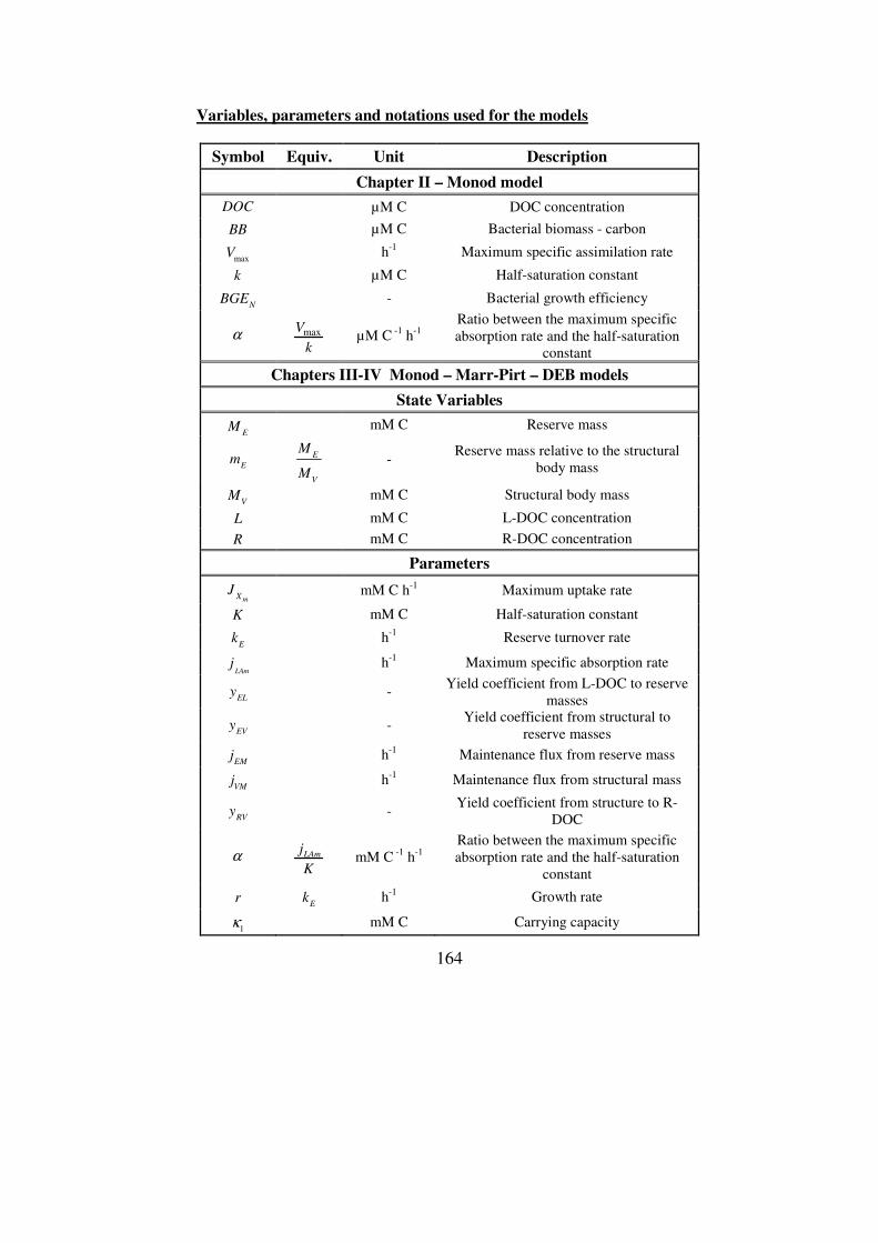
164
Variables, parameters and notations used for the models
Symbol Equiv. Unit Description
Chapter II – Monod model
DOC µM C DOC concentration
BB µM C Bacterial biomass - carbon
maxV h
-1 Maximum specific assimilation rate
k µM C Half-saturation constant
NBGE - Bacterial growth efficiency
α maxV
k µM C
-1 h
-1
Ratio between the maximum specific
absorption rate and the half-saturation
constant
Chapters III-IV Monod – Marr-Pirt – DEB models
State Variables
EM mM C Reserve mass
Em E
V
M
M -
Reserve mass relative to the structural
body mass
VM mM C Structural body mass
L mM C L-DOC concentration
R mM C R-DOC concentration
Parameters
mXJ mM C h
-1 Maximum uptake rate
K mM C Half-saturation constant
Ek h
-1 Reserve turnover rate
LAmj h
-1 Maximum specific absorption rate
ELy -
Yield coefficient from L-DOC to reserve
masses
EVy -
Yield coefficient from structural to
reserve masses
EMj h
-1 Maintenance flux from reserve mass
VMj h
-1 Maintenance flux from structural mass
RVy
-
Yield coefficient from structure to R-
DOC
α LAmj
K mM C
-1 h
-1
Ratio between the maximum specific
absorption rate and the half-saturation
constant
r E
k h-1
Growth rate
1κ mM C Carrying capacity
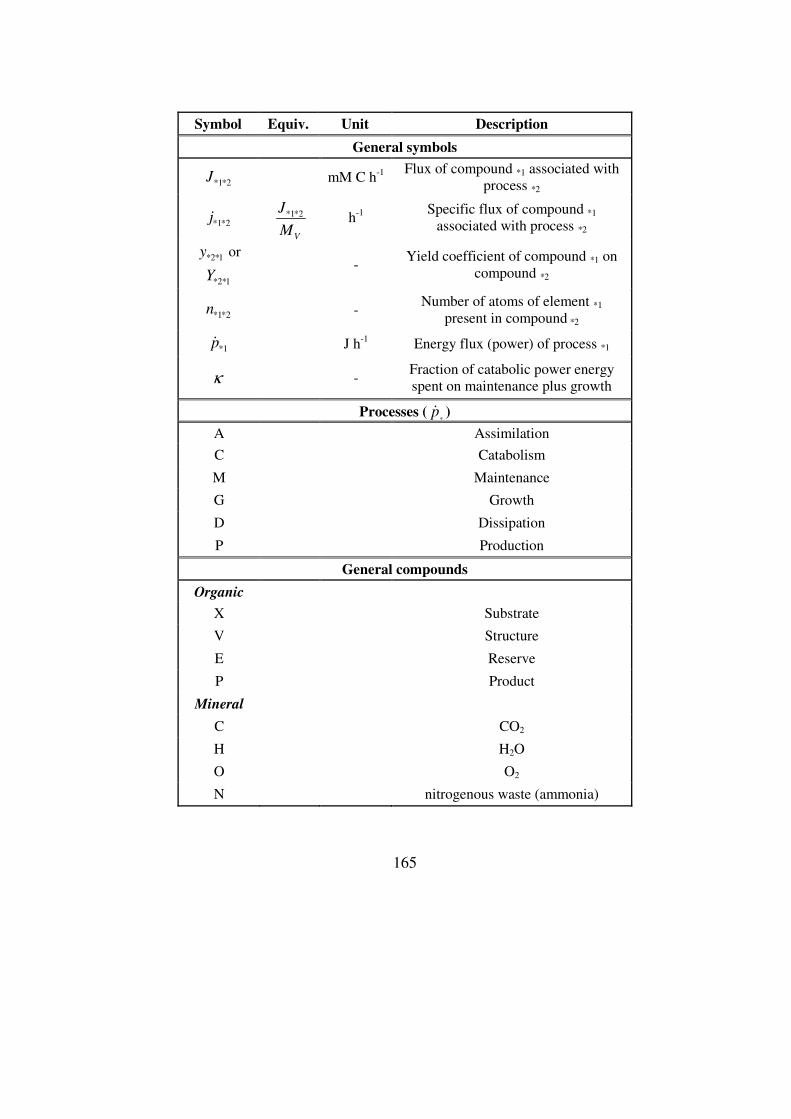
165
Symbol Equiv. Unit Description
General symbols
*1*2J
mM C h-1
Flux of compound *1 associated with
process *2
*1*2j *1*2
V
J
M h
-1
Specific flux of compound *1
associated with process *2
*2*1y or
*2*1Y -
Yield coefficient of compound *1 on
compound *2
*1*2n
- Number of atoms of element *1
present in compound *2
*1p� J h-1
Energy flux (power) of process *1
κ
- Fraction of catabolic power energy
spent on maintenance plus growth
Processes (*
p� )
A Assimilation
C Catabolism
M Maintenance
G Growth
D Dissipation
P Production
General compounds
Organic
X Substrate
V Structure
E Reserve
P Product
Mineral
C CO2
H H2O
O O2
N nitrogenous waste (ammonia)