_b-spline interpolation of soil water characteristic data

1 Introduction

Soil water characteristic data are commonly measured forsoil physical applications. To obtain values between mea-surements, empirical functions are typically fitted to thedata, e.g. the ones of VAN GENUCHTEN et al. (1991) orBROOKS and COREY. However, they assume a certain shapethat might not be appropriate for every data set. KASTANEK

and NIELSEN (2001) presented a computer program for theinterpolation of soil water characteristic data with naturalcubic spline functions. In addition, the use of so-called “vir-

tual data-points” enables the user to perform approxima-tion of these data by hand. In some cases, this was consid-ered necessary since cubic spline functions can exhibit sig-nificant oscillations between data points.

B-spline curves are piecewise polynomial parametriccurves commonly used in computer graphics. Some of theirfeatures could be of advantage with regard to the interpo-lation of soil water characteristic data, such as the local sup-port property.

Objective of this paper was to test the capabilities of thetechnique of B-spline curves to interpolate soil water char-

Die Bodenkultur 133 56 (2) 2005

B-Spline Interpolation of Soil Water Characteristic DataA. Schnepf and J. Hofmann

Interpolation von Matrixpotenzial-Wassergehaltsbeziehungen mit B-Splines

ZusammenfassungDie Matrixpotenzial-Wassergehaltsbeziehung ist eine Grundgröße für jegliche Berechnung von Wasserbewegung undanderen Größen des Wasserhaushalts. Werte zwischen den Messpunkten können durch Approximationen oder Inter-polationen berechnet werden. In der vorliegenden Arbeit wurde der mathematische Algorithmus der B-Spline Inter-polation und dessen Anwendung auf Matrixpotenzial-Wassergehaltsbeziehungen beschrieben. Ein Computerpro-gramm zur Interpolation mit Hilfe von B-Splines und natürlichen kubischen Splines wurde in JAVA 2 implementiert.Splines bieten vor allem dann eine hilfreiche Alternative, wenn es nicht möglich ist, empirische Gleichungen wie dievon VAN GENUCHTEN zu approximieren. Im Vergleich zu natürlichen kubischen Splines verhalten sich uniforme B-Splines zweiter und dritter Ordnung zwischen den Datenpunkten weniger oszillatorisch. Trotzdem garantieren sienicht, dass die Interpolationskurve der Monotonie der Daten folgt. Die lokale Veränderbarkeit von B-Splines, ohneden Rest der Kurve zu beeinflussen, kann hier genutzt werden.

Schlagworte: Wassergehalt, Boden, B-Splines, Wasserbewegung, Matrixpotenzial.

SummarySoil water characteristic data are of fundamental importance for all calculations of soil water movement. Valuesbetween measurements can be obtained by curve approximation or interpolation techniques. In this paper, the math-ematical algorithm of B-spline interpolation is described and its use for interpolation of soil water characteristic datais demonstrated. A computer program for interpolation with B-splines and natural cubic splines was implemented inJAVA 2. In cases were VAN GENUCHTEN equations cannot be fitted to the data with sufficient accuracy, splines pro-vide a helpful alternative. In comparison to natural cubic splines, uniform B-splines of degree 2 and 3 tend to exhib-it less oscillations between data points. However, they do not guarantee to follow the monotony of the data in all cases.The local modification property of B-splines can be used to adjust segments of the curve while the rest of the curvestays unchanged.

Key words: Soil water, B-Spline, Matric potential head.

acteristic data. A computer program for interpolation withnatural cubic splines and B-splines of various degrees andparametrizations was implemented in JAVA 2. Moving con-trol points results in local changes of the shape of the curve(local support property). This feature was implemented inthe JAVA 2 program allowing control points to be movedby mouse drags. This concept is similar to the concept ofthe virtual data points used by KASTANEK and NIELSEN

(2001). It is different by the fact that the curve can be modified in one segment while the rest of the curve stays unchanged. Results were compared to the results ofinterpolation with natural cubic spline functions as well ascurve fitting with the VAN GENUCHTEN equation (VAN

GENUCHTEN et al. 1991).

2 Material and Methods

2.1 Data Sets

The data sets for the soil water characteristics were obtainedfrom soil samples of a loamy silt from Mistelbach, 60 kmnorth of Vienna. They are part of an investigation on a longterm experimental field (FWF project P15329), where theinfluence of different tillage practices on soil quality isinvestigated. Three tillage systems are compared: Conven-tional tillage (CV), conservation tillage systems with covercrop during winter period (CS) and no-tillage systems withcover crop during winter period (NT). In fall 2002, afterthe harvest of mais, undisturbed samples where taken infour depths (0, 10, 25 and 50 cm) and two replicates foreach treatment, resulting in a total of 24 data sets. Eachvalue of each data set is again a mean of three replications.Samples were analyzed according to the Austrian standardÖNORM L1063 (1988). Data sets were analyzed andcleaned from obvious errors before interpolation.

2.2 Data Representation

Whether soil water characteristic data are referred to as θ(h)or h(θ) has an influence on the interpolation result in mostcases (except B-splines with uniform parametrization). Inthe following, the common θ(h) notation will be used (VAN

GENUCHTEN et al. 1991). Matric potential head of soil water characteristics is gener-

ally presented in both linear and log scale. Because transfor-mation of zero matric potential head into log scale is prob-

lematic, all interpolations were performed using originaldata values. In graph presentations, both scales were used.

2.3 Parametric B-Spline Curves – Theory

Natural cubic splines and VAN GENUCHTEN’s equation aredescribed in KASTANEK and NIELSEN (2001). In the follow-ing, we describe in detail the theory of parameteric B-splinecurves.

B-spline curves are piecewise polynomial parametriccurves of degree p. A B-spline curve with n+1 control pointsis defined as

(1)

where p � N is the degree of the B-spline curve, Ni,p � Rare the B-spline basis functions and Pi � R2 are the associ-ated control points.

The B-Spline basis functions can be defined recursivelyby the equation of COX-DE BOOR, Eq. (2),

(2)

Significant features of B-splines Bp(u) are (DE BOOR 1978):1. Ni,p(u) is a polynomial of order p in u,2. For all i, p and u is Ni,p(u) non-negative,3. Ni,p(u) is equal to zero except for the interval [ui, ui+1)

(local support),4. On the interval [ui, ui+1), only p+1 basis functions of

order p are not equal zero, namely, Ni-p,p(u),Ni-p+1,p(u), ..., Ni,p(u),

5. Ni,p(u) � Cp-k at knots with multiplicity k.

The third property can be used to modify interpolationcurves of soil water characteristics locally while the rest ofthe curve stays unchanged.

2.3.1 Global Curve Interpolation

We wish to find a B-spline curve of degree p that passes

through n+1 given data points

From these, the curve parameters t0, t1, ..., tn and the knotvector U = (u0, u1, ..., um) have to be determined, withm=n+p+1.


A. Schnepf and J. Hofmann

Common parametrization methods are the uniformlyspaced method, the cord length method and the centripetalmethod. We define the cord length method according toSPÄTH (1983):

(3)

whereThe uniformly spaced method is defined by dividing the

domain [x0, xn] into equal subintervals,

(4)

The behavior of a curve based on this parametrization couldbe described by a car which drives in such a way that thetime spent between points is constant. If the points are farenough away, the speed is relatively fast and might causeproblems around sharp corners. The cord length parame-trization shown in Eq. (3) can also cause problems aroundsharp corners.

The centripetal method is given by

(5)

where

B-spline curves are defined in terms of u. The intervalbetween two elements of the knot vector U in which u liesdetermines which control points determine the shape of thecurve. There are several methods to determine the m+p+1knots. Knots can also be uniformly spaced, such a knot vec-tor does not need knowledge of the parameters. However,this method is not recommended when used with the cordlength method for global interpolation, because the result-ing system of linear equations would be singular. Anotherway for generating knot vectors is:

(6)

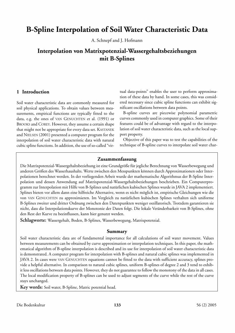
Figure 1: Cubic B-Spline interpolation (a) clamped and (b) un-clamped

Abbildung 1: Interpolation mit kubischen Splines (a) eingespannt (b)nicht eingespannt.

Knot vectors where the first and last knot have multiplicityp+1 are called clamped, the corresponding B-spline curve istangent to the first and the last legs at the first and last con-trol points. B-spline curves calculated from “un-clamped”vectors do not pass through the first and last data point andwill therefore not be considered for interpolation of soilwater characteristic data (see Figure 1).

Let N be a (n+1) × (n+1) matrix containing the values ofthe B-spline basis functions for the parameter values calcu-lated with Eq. (2),

(7)

Let the given data points and the yet unknown controlpoints be presented in matrix form

(8)

B-Spline Interpolation of Soil Water Characteristic Data


Then P can be obtained from the system of equations

D = NP. (9)

Knowing control points and knot vector allows to calculatepoints on the B-spline curve between the data points usingDE BOOR’s algorithm. As input, it needs a u ∈ R that liesbetween two elements of the knot vector U, output is apoint on the curve Bp(u). The interval in which u lies deter-mines the p+1 control points that influence this particularcurve segment.

3 Results and Discussion

3.1 Selection of B-spline type

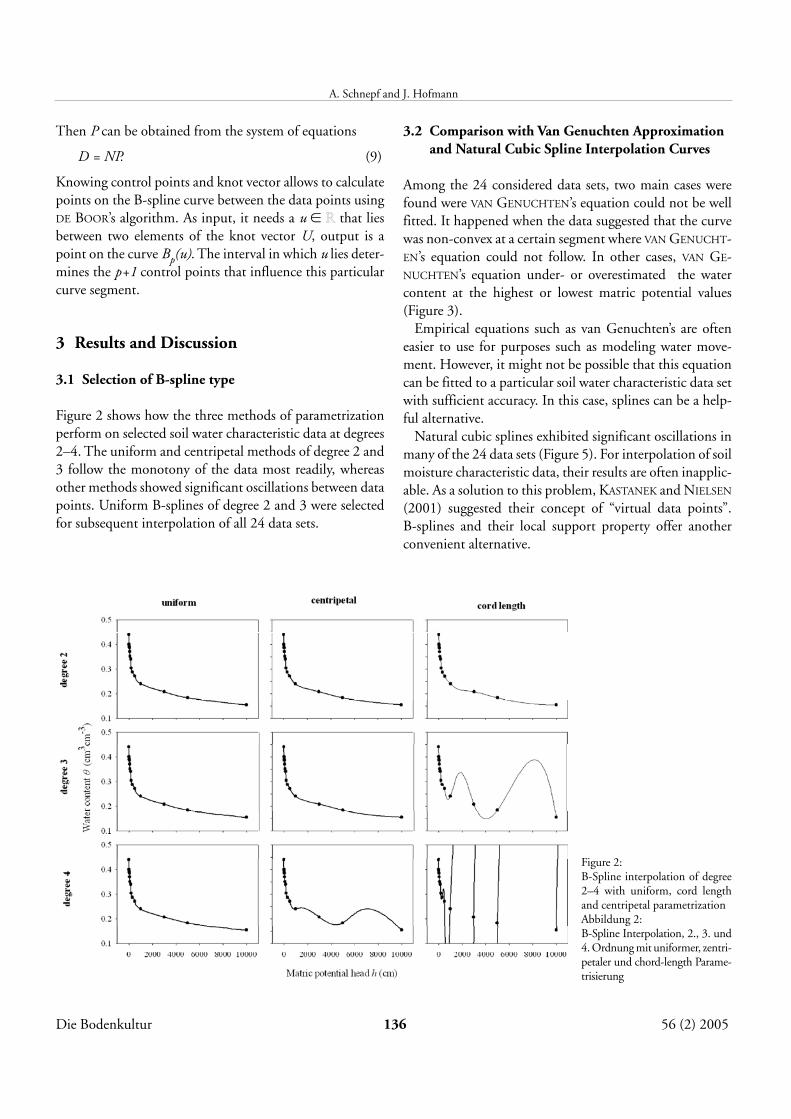
Figure 2 shows how the three methods of parametrizationperform on selected soil water characteristic data at degrees2–4. The uniform and centripetal methods of degree 2 and3 follow the monotony of the data most readily, whereasother methods showed significant oscillations between datapoints. Uniform B-splines of degree 2 and 3 were selectedfor subsequent interpolation of all 24 data sets.

3.2 Comparison with Van Genuchten Approximationand Natural Cubic Spline Interpolation Curves

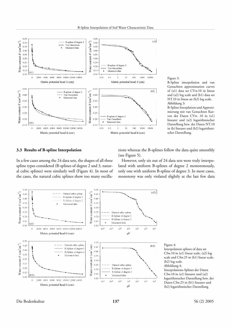
Among the 24 considered data sets, two main cases werefound were VAN GENUCHTEN’s equation could not be wellfitted. It happened when the data suggested that the curvewas non-convex at a certain segment where VAN GENUCHT-EN’s equation could not follow. In other cases, VAN GE-NUCHTEN’s equation under- or overestimated the watercontent at the highest or lowest matric potential values (Figure 3).

Empirical equations such as van Genuchten’s are ofteneasier to use for purposes such as modeling water move-ment. However, it might not be possible that this equationcan be fitted to a particular soil water characteristic data setwith sufficient accuracy. In this case, splines can be a help-ful alternative.

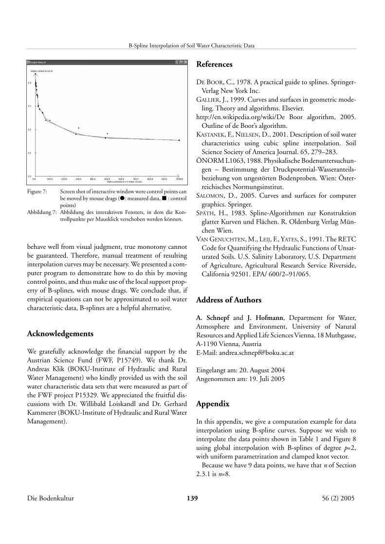
Natural cubic splines exhibited significant oscillations inmany of the 24 data sets (Figure 5). For interpolation of soilmoisture characteristic data, their results are often inapplic-able. As a solution to this problem, KASTANEK and NIELSEN

(2001) suggested their concept of “virtual data points”. B-splines and their local support property offer anotherconvenient alternative.



Figure 2: B-Spline interpolation of degree2–4 with uniform, cord lengthand centripetal parametrizationAbbildung 2:B-Spline Interpolation, 2., 3. und4. Ordnung mit uniformer, zentri-petaler und chord-length Parame-trisierung

3.3 Results of B-spline Interpolation

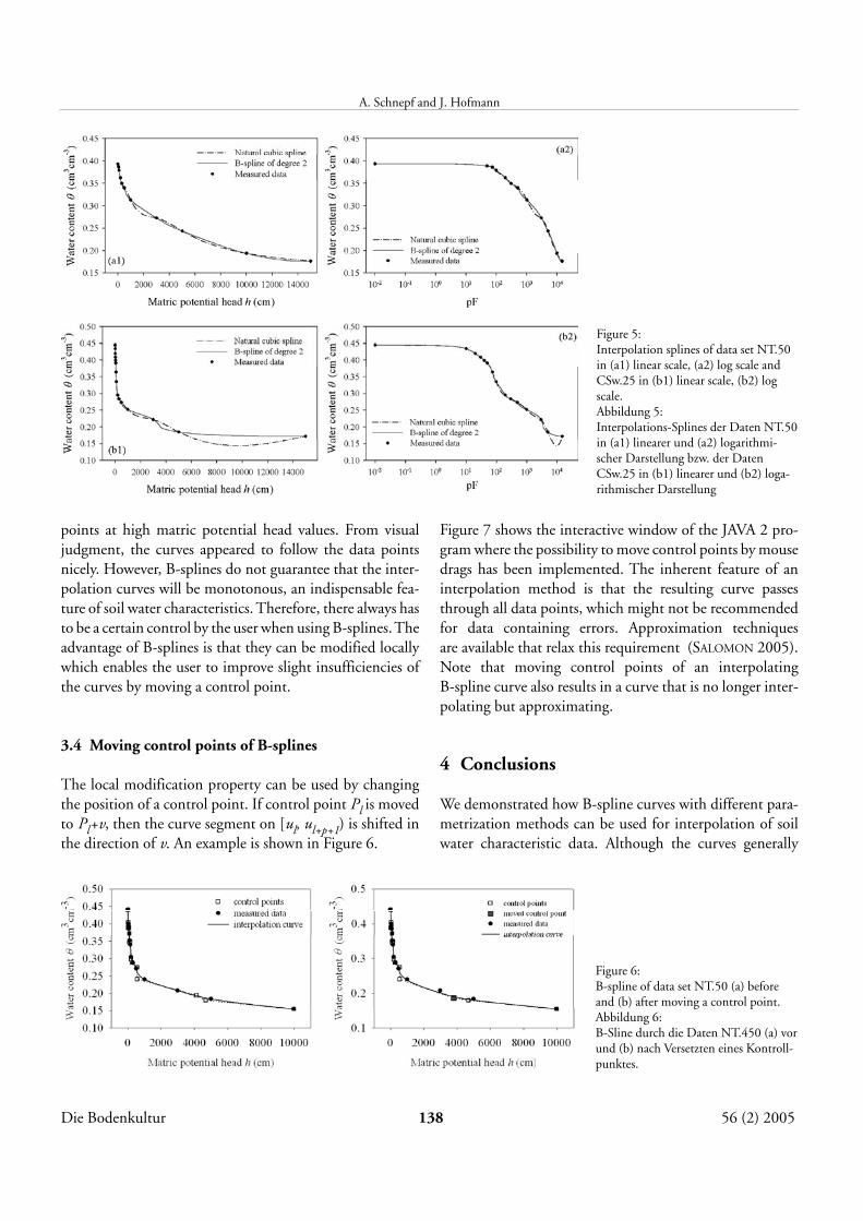
In a few cases among the 24 data sets, the shapes of all threespline types considered (B-splines of degree 2 and 3, natur-al cubic splines) were similarly well (Figure 4). In most ofthe cases, the natural cubic splines show too many oscilla-

tions whereas the B-splines follow the data quite smoothly(see Figure 5).

However, only six out of 24 data sets were truly interpo-lated with uniform B-splines of degree 2 monotonously,only one with uniform B-spline of degree 3. In most cases,monotony was only violated slightly at the last few data



Figure 3: B-Spline interpolation and vanGenuchten approximation curvesof (a1) data set CVw.10 in linearand (a2) log scale and (b1) data setNT.10 in linear an (b2) log scale.Abbildung 3: B-Spline Interplation und Approxi-mierung mit van Genuchten Kur-ven der Daten CVw. 10 in (a1)linearer und (a2) logarithmischerDarstellung bzw. der Daten NT.10in (b) linearer und (b2) logarithmi-scher Darstellung.

Figure 4: Interpolation splines of data setCSw.10 in (a1) linear scale, (a2) logscale and CSw.25 in (b1) linear scale,(b2) log scale.Abbildung 4:Interpolations-Splines der DatenCSw.10 in (a1) linearer und (a2)logarithmischer Darstellung bzw. derDaten CSw.25 in (b1) linearer und(b2) logarithmischer Darstellung

points at high matric potential head values. From visualjudgment, the curves appeared to follow the data pointsnicely. However, B-splines do not guarantee that the inter-polation curves will be monotonous, an indispensable fea-ture of soil water characteristics. Therefore, there always hasto be a certain control by the user when using B-splines. Theadvantage of B-splines is that they can be modified locallywhich enables the user to improve slight insufficiencies ofthe curves by moving a control point.

3.4 Moving control points of B-splines

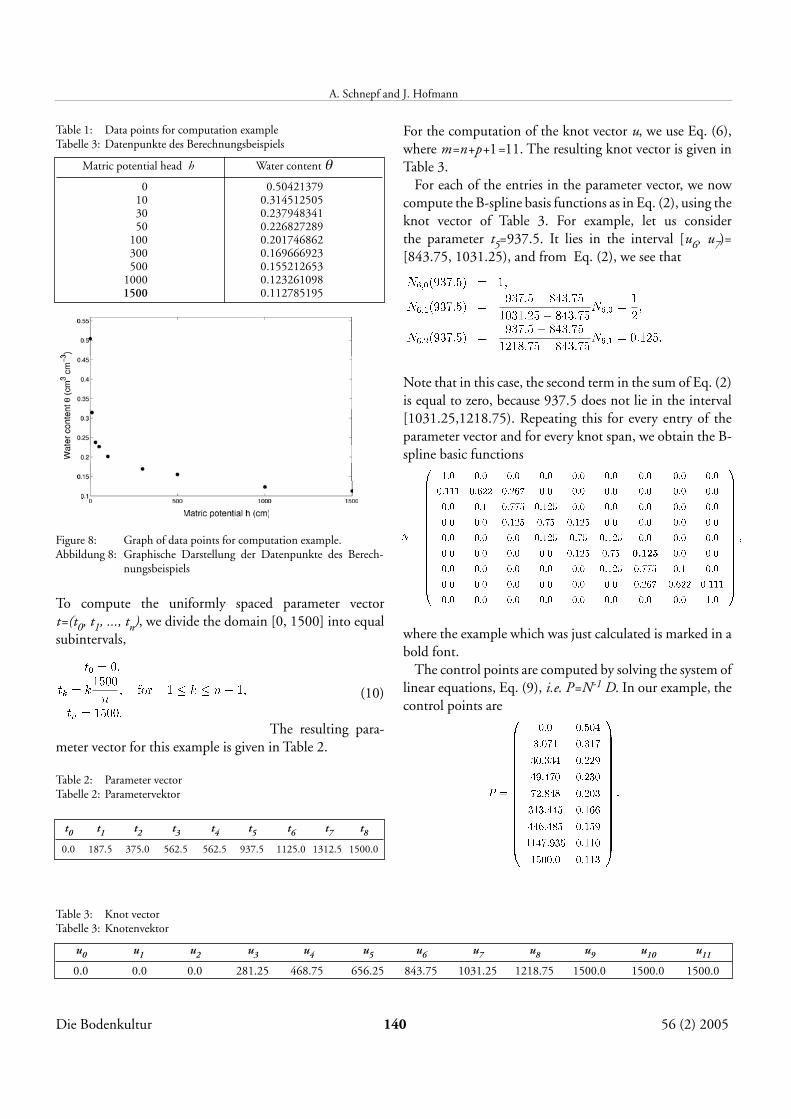
The local modification property can be used by changingthe position of a control point. If control point Pl is movedto Pl+v, then the curve segment on [ul, ul+p+1) is shifted inthe direction of v. An example is shown in Figure 6.

Figure 7 shows the interactive window of the JAVA 2 pro-gram where the possibility to move control points by mousedrags has been implemented. The inherent feature of aninterpolation method is that the resulting curve passesthrough all data points, which might not be recommendedfor data containing errors. Approximation techniques are available that relax this requirement (SALOMON 2005).Note that moving control points of an interpolating B-spline curve also results in a curve that is no longer inter-polating but approximating.

4 Conclusions

We demonstrated how B-spline curves with different para-metrization methods can be used for interpolation of soilwater characteristic data. Although the curves generally



Figure 5: Interpolation splines of data set NT.50in (a1) linear scale, (a2) log scale andCSw.25 in (b1) linear scale, (b2) logscale.Abbildung 5:Interpolations-Splines der Daten NT.50in (a1) linearer und (a2) logarithmi-scher Darstellung bzw. der DatenCSw.25 in (b1) linearer und (b2) loga-rithmischer Darstellung

Figure 6: B-spline of data set NT.50 (a) beforeand (b) after moving a control point.Abbildung 6:B-Sline durch die Daten NT.450 (a) vorund (b) nach Versetzten eines Kontroll-punktes.

behave well from visual judgment, true monotony cannotbe guaranteed. Therefore, manual treatment of resultinginterpolation curves may be necessary. We presented a com-puter program to demonstrate how to do this by movingcontrol points, and thus make use of the local support prop-erty of B-splines, with mouse drags. We conclude that, ifempirical equations can not be approximated to soil watercharacteristic data, B-splines are a helpful alternative.

Acknowledgements

We gratefully acknowledge the financial support by theAustrian Science Fund (FWF, P15749). We thank Dr.Andreas Klik (BOKU-Institute of Hydraulic and RuralWater Management) who kindly provided us with the soilwater characteristic data sets that were measured as part ofthe FWF project P15329. We appreciated the fruitful dis-cussions with Dr. Willibald Loiskandl and Dr. GerhardKammerer (BOKU-Institute of Hydraulic and Rural WaterManagement).

References

DE BOOR, C., 1978. A practical guide to splines. Springer-Verlag New York Inc.

GALLIER, J., 1999. Curves and surfaces in geometric mode-ling. Theory and algorithms. Elsevier.

http://en.wikipedia.org/wiki/De Boor algorithm, 2005.Outline of de Boor’s algorithm.

KASTANEK, F., NIELSEN, D., 2001. Description of soil watercharacteristics using cubic spline interpolation. Soil Science Society of America Journal. 65, 279–283.

ÖNORM L1063, 1988. Physikalische Bodenuntersuchun-gen – Bestimmung der Druckpotential-Wasseranteils-beziehung von ungestörten Bodenproben. Wien: Öster-reichisches Normungsinstitut.

SALOMON, D., 2005. Curves and surfaces for computergraphics. Springer.

SPÄTH, H., 1983. Spline-Algorithmen zur Konstruktionglatter Kurven und Flächen. R. Oldenburg Verlag Mün-chen Wien.

VAN GENUCHTEN, M., LEIJ, F., YATES, S., 1991. The RETCCode for Quantifying the Hydraulic Functions of Unsat-urated Soils. U.S. Salinity Laboratory, U.S. Departmentof Agriculture, Agricultural Research Service Riverside,California 92501. EPA/ 600/2–91/065.

Address of Authors

A. Schnepf and J. Hofmann, Department for Water,Atmosphere and Environment, University of NaturalResources and Applied Life Sciences Vienna, 18 Muthgasse,A-1190 Vienna, AustriaE-Mail: [email protected]

Eingelangt am: 20. August 2004Angenommen am: 19. Juli 2005

Appendix

In this appendix, we give a computation example for datainterpolation using B-spline curves. Suppose we wish tointerpolate the data points shown in Table 1 and Figure 8using global interpolation with B-splines of degree p=2,with uniform parametrization and clamped knot vector.

Because we have 9 data points, we have that n of Section2.3.1 is n=8.



Figure 7: Screen shot of interactive window were control points canbe moved by mouse drags (�: measured data, � : controlpoints)

Abbildung 7: Abbildung des interaktiven Fensters, in dem die Kon-trollpunkte per Mausklick verschoben werden können.

To compute the uniformly spaced parameter vector t=(t0, t1, ..., tn), we divide the domain [0, 1500] into equalsubintervals,

(10)

The resulting para-meter vector for this example is given in Table 2.

Table 2: Parameter vectorTabelle 2: Parametervektor

For the computation of the knot vector u, we use Eq. (6),where m=n+p+1=11. The resulting knot vector is given inTable 3.

For each of the entries in the parameter vector, we nowcompute the B-spline basis functions as in Eq. (2), using theknot vector of Table 3. For example, let us consider the parameter t5=937.5. It lies in the interval [u6, u7)=[843.75, 1031.25), and from Eq. (2), we see that

Note that in this case, the second term in the sum of Eq. (2)is equal to zero, because 937.5 does not lie in the interval[1031.25,1218.75). Repeating this for every entry of theparameter vector and for every knot span, we obtain the B-spline basic functions

where the example which was just calculated is marked in abold font.

The control points are computed by solving the system oflinear equations, Eq. (9), i.e. P=N-1 D. In our example, thecontrol points are



Matric potential head h Water content θ0 0.50421379

10 0.314512505 30 0.237948341 50 0.226827289

100 0.201746862 300 0.169666923 500 0.155212653

1000 0.123261098 1500 0.112785195

t0 t1 t2 t3 t4 t5 t6 t7 t8

0.0 187.5 375.0 562.5 562.5 937.5 1125.0 1312.5 1500.0

Figure 8: Graph of data points for computation example.Abbildung 8: Graphische Darstellung der Datenpunkte des Berech-

nungsbeispiels

Table 3: Knot vectorTabelle 3: Knotenvektor

u0 u1 u2 u3 u4 u5 u6 u7 u8 u9 u10 u11

0.0 0.0 0.0 281.25 468.75 656.25 843.75 1031.25 1218.75 1500.0 1500.0 1500.0

Table 1: Data points for computation exampleTabelle 3: Datenpunkte des Berechnungsbeispiels

The points on the B-spline curve between the data pointsare computed using de Boor’s algorithm (GALLIER 1999).In the following, we present its outline as shown athttp://en.wikipedia.org/wiki/De_Boor_algorithm (2005):

Input: a value uOutput: the point on the curve, B(u)

Let u lie in [uk,uk+1), with u ≠ uk, and let p be the degree ofthe B-spline curve;Copy the affected control points Pk, Pk-1, Pk-2, ..., Pk-p+1 andPk-p to a new array and rename them Pk,0, Pk-s-1,0, Pk-2,0, ..., Pk-p+1,0 and Pk-p,0;for r := 1 to p dofor i := k-p+r to k dobeginLet ai,r = (u - ui) / ( ui+p-r+1 - ui)Let Pi,r = (1 - ai,r) Pi-1,r-1 + ai,r Pi,r-1endPk,p is the point B(u).

Suppose we wish to calculate the point on the B-splinecurve that corresponds to u=164.4518. This value lies in theinterval [u2, u3)=[0.0, 281.25); remember that the degreep=2. The affected control points are P0, P1 and P2, and werename them P0,0, P1,0 and P2,0. The computation of thepoint on the curve is illustrated in Fig. 9.

We compute the second column, P1,1 and P2,1 as follows:The coefficients a1,1 and a2,1 are

and

The coefficient for the computation of the third column,a2,2, is

and

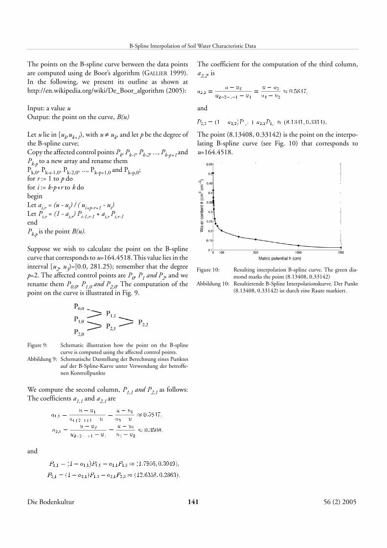
The point (8.13408, 0.33142) is the point on the interpo-lating B-spline curve (see Fig. 10) that corresponds tou=164.4518.



Figure 9: Schematic illustration how the point on the B-splinecurve is computed using the affected control points.

Abbildung 9: Schematische Darstellung der Berechnung eines Punktesauf der B-Spline-Kurve unter Verwendung der betroffe-nen Kontrollpunkte

Figure 10: Resulting interpolation B-spline curve. The green dia-mond marks the point (8.13408, 0.33142)

Abbildung 10: Resultierende B-Spline Interpolationskurve. Der Punkt(8.13408, 0.33142) ist durch eine Raute markiert.

_b-spline interpolation of soil water characteristic data

Documents